Comparison of Linear and Nonlinear Ultrasonic Features for the Analysis of Concrete Under Compression

Abstract

The early detection and monitoring of stress-induced damage in concrete is a key goal for nondestructive evaluation and structural health monitoring of civil structures. Both linear and nonlinear ultrasonic testing methods have been developed for this purpose. The Ultrasonic Pulse Velocity (UPV) test is the standard linear technique and is reliable and easy to use, but it typically detects defects only after micro-cracks coalesce or grow beyond a threshold size. To enable earlier detection, features extracted from the nonlinear ultrasonic response—especially harmonics generation—have been proposed. However, these approaches often require complex measurement protocols, and their signal-to-noise ratio (SNR) can be limited. In this study, we leverage an exponential swept-sine pulse-compression (ESS–PuC) procedure to characterize both linear and nonlinear responses from a single measurement. We define and extract several features from both responses, and use them to monitor micro-crack initiation and growth in concrete specimens under gradually increasing compressive load. This enables a qualitative comparison of their characteristics and performance in detecting crack formation.

1. Introduction

Concrete is the most used material in the construction of buildings and civil infra-structures [1] due to its mechanical and thermal properties, cost effectiveness, capability of being realized in complex shapes, and the ability to tune its properties via composition or reinforcement. However, excessive loading and other damaging conditions can lead to the generation of micro-cracks and defects that reduce mechanical properties and durability. Developing nondestructive evaluation (NDE) and structural health monitoring (SHM) strategies able to detect micro-crack generation and estimate residual life is thus of the utmost importance, and a large multidisciplinary research effort has focused on this aim for several decades [2,3,4,5]. Contextually, the physics of concrete cracking is studied through numerical simulations at the micro- and meso scale to clarify crack initiation/growth scenarios, and supporting the interpretation of NDE and SHM data [6,7].

Among the NDE methods, various ultrasonic (UT) techniques have been developed to monitor and evaluate the condition of concrete structures, including both linear and nonlinear methods. Typical features extracted from the linear UT response include time-of-flight (ToF), attenuation, spectral peak, and frequency-dependent attenuation; these features are used to monitor and assess macro-properties of the structures and to detect damage. In particular, the standard test for the evaluation of concrete’s quality is the Ultrasonic Pulse Velocity (UPV), which relates the sound velocity value measured between a transmitter and a receiver transducer with the mean degree of concrete quality [8,9]. Macro-cracks and voids can also be detected by UPV, as they lengthen the effective travel path between the transducers. The wave velocity decreases as well due to micro-crack density, indicating a reduction in the material’s effective elastic modulus. However, the ToF extracted from the linear response often remains unchanged at the initial stages of micro-level damage and only shows significant changes once the damage surpasses a certain extent [10].

This lack of sensitivity is further aggravated from the fact that very narrowband transducers are usually employed to achieve larger SNR, thus limiting the available information. For this reason, in [11] a broadband capacitive micromachined ultrasonic transducer is proposed to increase the sensitivity of UPV.

Besides ToF, attenuation provides insight into energy loss due to refraction and scattering within the material, and thus it can also be used to assess the density of micro-cracks and the presence of large reflectors such as cracks, aggregates, voids. However, it suffers from the variability in the coupling between transducers and the sample under test. To mitigate this, in [12], the features extracted from the temporal distribution of the energy of the UT signals are proposed to detect the presence of defects.

At the same time, UT measurement procedures relying on the extraction of features from the nonlinear acoustic response of concrete caused by its stress–strain nonlinearity or by the presence of defects inducing nonlinear ultrasonic behavior have been developed in the last decades. These methods have shown enhanced sensitivity to micro-cracks and load-induced damage with respect to UPV, thus allowing the inherent nonlinear mechanical behavior of concrete materials to be investigated [13,14,15,16,17].

Nonlinear ultrasonic (NL-UT) tests often measure the generation of higher harmonics, sub-harmonics or wave mixing [18], nonlinear resonance [19], and involve performing measurements with different signal amplitudes and with narrowband excitation as in the Scaling Subtraction Method (SSM) [13], or with multiple transducers as in [20].

In this paper, we tailor and optimize for concrete inspection a method developed by Angelo Farina to simultaneously characterize the acoustic impulse response and the distortion of an audio component [21]. This method is now standard and widely applied in environmental/room acoustics and audio systems [22,23,24,25], and it has also been used in vibrational analysis [26,27,28] and in system analysis [29,30], and early results of its application to concrete sample from some of the present authors are also reported in [31]. With respect previous applications of NL-UT, here several features are defined and extracted from both linear and nonlinear system responses starting from the result of a single measurement. The method leverages pulse compression to increase the SNR of the measurement without overly increasing the excitation amplitude, or without doing many averages. The broadband excitation instead makes it possible to characterize for each harmonic not just some numerical coefficients but a set of functions, from which several features can be extracted as in this case.

To evaluate the sensitivity and effectiveness of the method in detecting damaging of the concrete specimens under gradual increasing in the compression load, it has been applied on several specimens, and the results from six selected samples corresponding to three different mixtures have been compared.

The paper is organized as follows: in Section 2, the measurement procedure and the features extraction process are introduced. Section 3 describes the experimental setup and the procedure implemented and compares the various features. Section 4 discusses the results and perspectives, and draws some conclusions.

2. Materials and Methods

2.1. Exponential Swept-Sine Pulse Compression

Since Farina’s seminal work [21], the exponential swept-sine (ESS) pulse compression (PuC) technique has been used to characterize nonlinear systems that can well be modeled using a sum of a linear term and multiple Hammerstein systems acting in parallel, where each Hammerstein model consists of a static nonlinearity followed by a convolution operation, while the linear term involves only a convolution operation. Although many nonlinear systems, such as those exhibiting strong hysteretic behavior, cannot be accurately characterized using this approach, the multi-branch parallel Hammerstein model is effective in representing many physical phenomena and NDE applications, including environmental acoustics and vibration analysis. In this paper, this approach is adopted for the ultrasonic inspection of concrete, and the ESS-PuC procedure is used to identify the model allowing for both linear and nonlinear features extraction. Note that, although concrete exhibits a hysteretic behavior in its stress–strain ($\sigma -ϵ$) response under cyclic loading, the ESS procedure, as most of the other NL-UT techniques, tests the sample around a specific point of the $\sigma -ϵ$ curve. The hysteretic behavior can then be studied by monitoring the NL-UT extracted features under cyclic loading. In this perspective, the ESS-PuC is very promising, as it outputs not just numerical coefficients to quantify the nonlinearity but several 1D signals, whose time waveform can vary due to hysteresis.

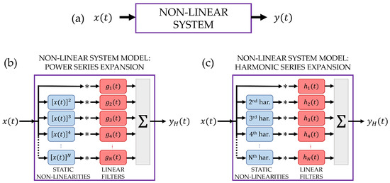
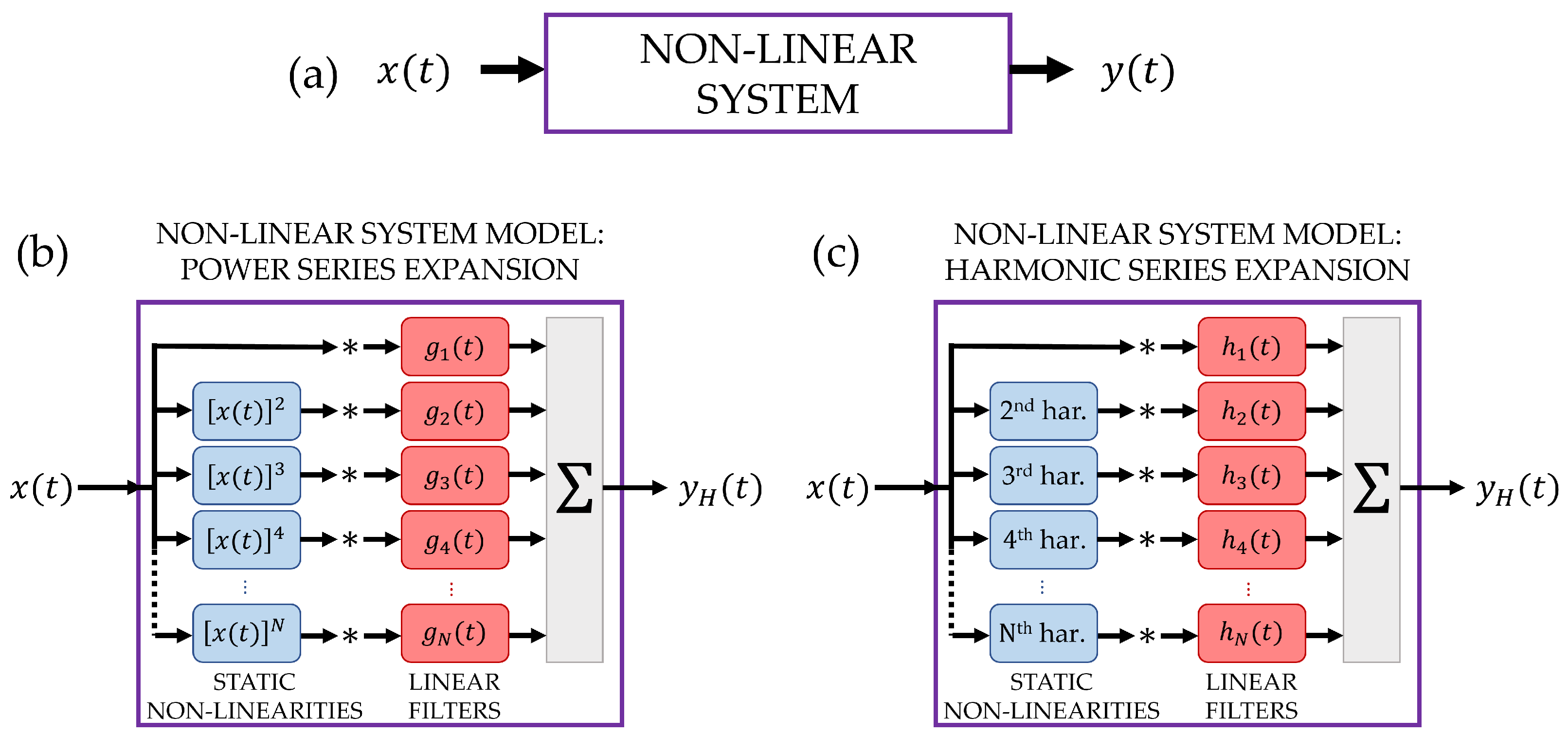
For the design of the ESS excitation signal and the matched filters, we followed the theoretical formulation detailed in references [24,32] and further refined in [33] with the introduction of an optimal reactance tapering window for ESS [34]. The basic principle of the identification procedure is illustrated in Figure 1: a nonlinear system (Figure 1a) is excited with the ESS signal $x\left(t\right)$ and outputs the signal $y\left(t\right)$; the system is modeled by a sum of a linear term and several Hammerstein blocks, all operating in parallel. This sum produces the estimate $y_H\left(t\right)$ of the true system output $y\left(t\right)$. There are two main approaches for expressing the parallel branches: (Figure 1b) the power series expansion, where static nonlinearities are represented by different powers of the input signal, and (Figure 1c) the harmonic series expansion, where nonlinear terms correspond to the generation of harmonics of the input signal. In the power series version, the various terms ${\left[x\left(t\right)\right]}^n$—including the linear term $n=1$—are filtered by a bank of filters, each characterized by an impulse response $\left\{g_n\left(t\right)\right\}$. Similarly, in the harmonic series expansion, the various harmonics, including the fundamental one, are filtered by a bank of filters, each characterized by an impulse response $\left\{h_n\left(t\right)\right\}$. Note that the fundamental harmonic and the $n=1$ power series term coincide.

Figure 1. Basic principle of the nonlinear system identification through a multi-branch parallel Hammerstein model: the input–output relationship of a generic nonlinear system is modeled as the sum of multiple Hammerstein models acting in parallel. Each Hammerstein model includes a static nonlinear term followed by a convolution operation, represented by the symbol “∗”. Two main approaches can be adopted for expressing the parallel branches: (b) the power series expansion, where static nonlinearities are represented by different powers of the input signal, and (c) the harmonic series expansion, where nonlinear terms correspond to the generation of harmonics of the input signal. In both cases, the branch (a) does not include any nonlinearity and represents the linear response of the system.

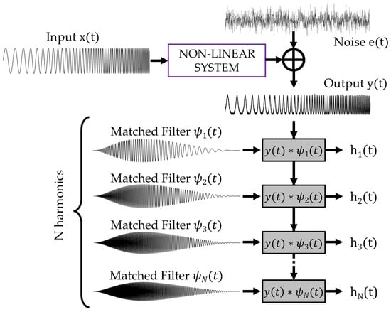
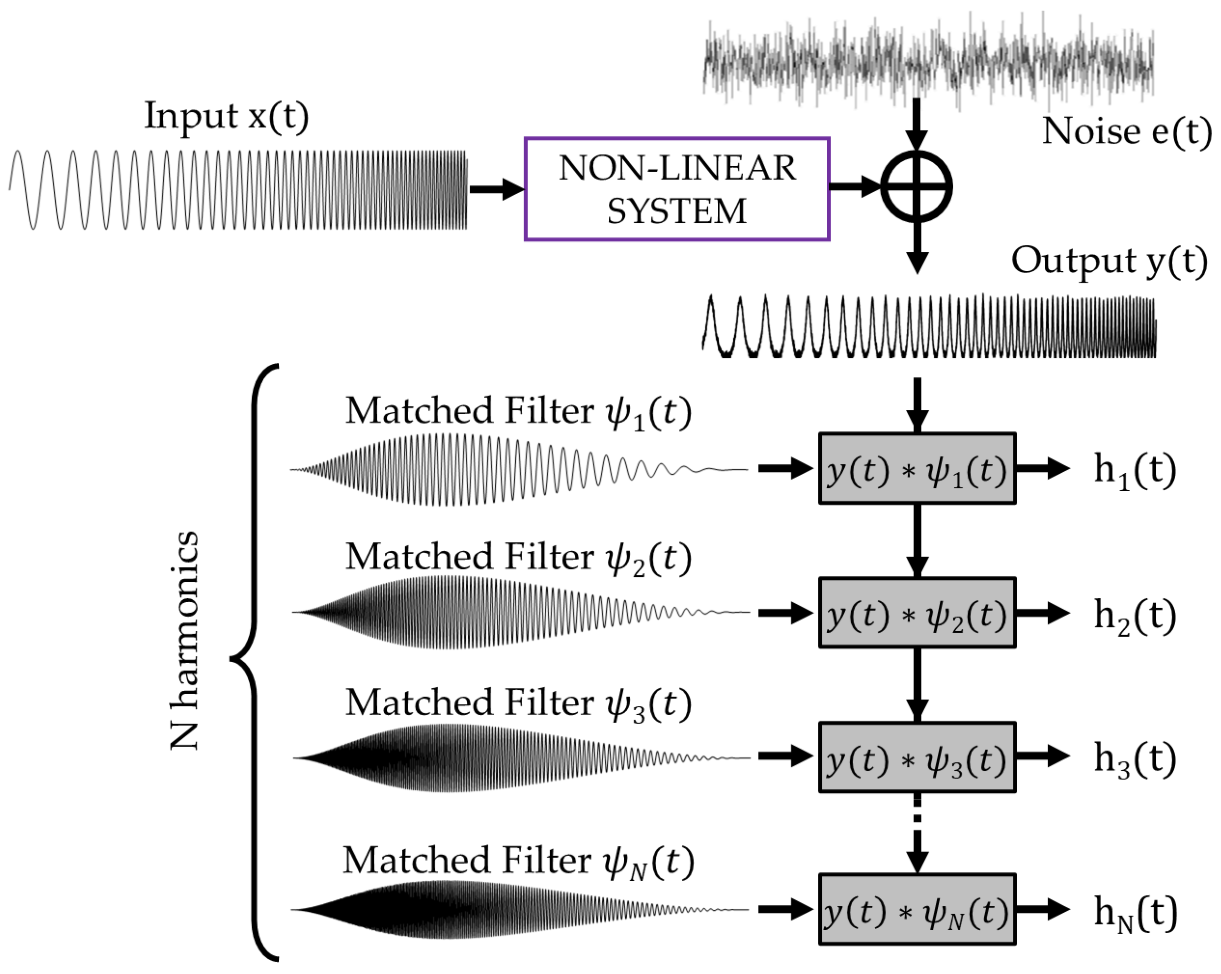
It is possible to transition from one representation to the other, as the harmonics can be expressed as a linear combination of powers, and vice versa. In particular, in the ESS-PuC procedure where the input is a cosine signal $x\left(t\right)=cos\left(\theta \left(t\right)\right)$, the n-th harmonic is associated to the n-th Chebyshev polynomial ${\mathcal{T}}_n(·)$ of the first kind defined by ${\mathcal{T}}_n(cos\left(\theta \left(t\right)\right)=cos\left(n\theta \left(t\right)\right)$; see [24]. Examples of ${\mathcal{T}}_n(·)$ are ${\mathcal{T}}_1\left(x\right)=x$, ${\mathcal{T}}_2\left(x\right)=2x^2-1$, ${\mathcal{T}}_3\left(x\right)=4x^3-3x$, ${\mathcal{T}}_4\left(x\right)=8x^4-8x^2+1$, etc. The possibility of changing representation is also guaranteed by the fact that the sets of $\left\{g_n\left(t\right)\right\}$ and $\left\{h_n\left(t\right)\right\}$ are connected to each other through a linear transformation as described in [26]. The optimal representation depends thus on the specific problem. In the present work, the harmonic series expansion is used, as many other works on the nonlinear ultrasound NDT of concrete structures analyze the harmonics generation. Furthers, the $\left\{h_n\left(t\right)\right\}$ are reconstructed one by one, by filtering the system output $y\left(t\right)$ with a specific matched filter $\left\{{\psi }_n\left(t\right)\right\}$ as illustrated in Figure 2.

Figure 2. Sketch of the ESS-PuC procedure: the ESS input signal $x\left(t\right)$ excites the sample, modeled as a nonlinear system. The noisy output signal is convolved with a bank of matched filters $\left\{{\psi }_{n\in \{1\dots N\}}\left(t\right)\right\}$ to reconstruct the impulse responses $\left\{h_n\left(t\right)\right\}$ associated to the various harmonics, where the symbol “∗” stands for the convolution operation. Note that the convolution with the matched filters implements the pulse-compression operation.

At the heart of the procedure is the definition of the input ESS signal $x\left(t\right)$, which is a cosine function of duration T with an argument varying exponentially with time:

$$\begin{array}{cc}\hfill x\left(t\right)& =cos\left(\theta \right(t\left)\right)\left[u\right(t)-u(t-T\left)\right]=\hfill \\ \hfill & =cos(2\pi f_{1}L[e^{t/L}-1]+{\theta }_0)[u\left(t\right)-u(t-T)]\hfill \\ \hfill & =ESS(t,f_1,f_2,{\theta }_0,T)\hfill \end{array}$$

(1)

In Equation (1), $\theta \left(t\right)$ and ${\theta }_0$ are the instantaneous and initial phases, respectively, $u\left(t\right)$ is the Heaviside step function, $f_1$ and $f_2$ are the lower and upper bounds of the swept frequency range, and $L=T/ln(f_2/f_1)$. The ESS bandwidth is $B_1=f_2-f_1$, while its instantaneous frequency $f_i\left(t\right)$ is derived by the instantaneous phase as

$$f_i\left(t\right)={\displaystyle \frac{1}{2\pi }}{\displaystyle \frac{d\theta \left(t\right)}{dt}}=f_1{e}^{t⁄L}$$

(2)

If $x\left(t\right)$ is the argument of a Chebyshev polynomial of the n-th degree, the result ${\mathcal{T}}_n\left(x\left(t\right)\right)$ is another ESS with the same T and $f_1^{\prime }=n{f}_1$,$f_2^{\prime }=n{f}_2$, ${\theta }_0^{\prime }=n{\theta }_0$, that coincides with the n-th harmonic of $x\left(t\right)$:

$$\begin{array}{cc}\hfill {\mathcal{T}}_n\left(ESS(t,f_1,f_2,{\theta }_0,T)\right)& =ESS(t,n{f}_1,n{f}_2,n{\theta }_0,T)=\hfill \\ \hfill & =cos(2\pi \left(n{f}_1\right)L[e^{t/L}-1]+n{\theta }_0)[u\left(t\right)-u(t-T)].\hfill \end{array}$$

(3)

Note that, if $f_1$, $f_2$ and ${\theta }_0$ are fixed, T cannot be arbitrary but must belong to a discrete set of values to assure that $x\left(t\right)$ and all the harmonics ${\mathcal{T}}_n\left(x\left(t\right)\right)$ are synchronized in phase [32,33]. It is also worth highlighting that while the envelope amplitude of $x\left(t\right)$ is almost constant, its spectrum is not flat: the power density is higher at low frequencies and decreases as the frequency increases. Precisely, the power spectrum decreases exponentially with the frequency so that each decade has an almost constant energy. ESS is indeed also called the logarithmic chirp.

The matched filter of the linear term is defined as

$$\begin{array}{cc}\hfill {\psi }_1\left(t\right)& =\left[x(T-t){\left({\displaystyle \frac{d{f}_i\left(t\right)}{dt}}\right)}^{-1}\right]w_R^{ESS}(t,f_1,f_2,T)=\hfill \\ \hfill & =ESS(T-t,f_1,f_2,{\theta }_0,T){\displaystyle \frac{L}{f_1}}{e}^{-t/L}{w}_R^{ESS}(t,f_1,f_2,T)\hfill \end{array}$$

(4)

where $w_R^{ESS}(t,f_1,f_2,T)$ is the reactance tapering window defined in [33]. ${\psi }_1\left(t\right)$ spans the same bandwidth of $x\left(t\right)$, but its envelope amplitude is not constant. Ignoring the window, the time-reversed input $x(T-t)$ is indeed amplitude modulated by the term ${\displaystyle \frac{L}{f_1}}{e}^{-t/L}$ so as to have an almost flat cross-power spectrum for $x\left(t\right)$ and ${\psi }_1\left(t\right)$ in the bandwidth $B_1=f_2-f_1$. This condition is needed to minimize the main lobe width of the convolution output ${\widehat{\delta }}_1=x\left(t\right)\ast {\psi }_1\left(t\right)$ [34], where ${\widehat{\delta }}_1$ is also called the resolution function of the pulse compression operation. The matched filter of the n-th harmonic term is nothing but the matched filter of the ESS ranging from $n{f}_1$ to $n{f}_2$, having as the initial phase $n{\theta }_0$, that is

$${\psi }_n\left(t\right)=[ESS(T-t,n{f}_1,n{f}_2,n{\theta }_0,T){\displaystyle \frac{L}{n{f}_1}}{e}^{-t/L}{w}_R^{ESS}(t,n{f}_1,n{f}_2,T)].$$

(5)

It is worth noting that for the peculiar properties of the exponential chirp, the set of ESS signals and related matched filters have common traits:

• All the instantaneous frequency functions of the various $ESS(t,n{f}_1,n{f}_2,n{\theta }_0,T)$ signals have the same coefficient $1/L$ for the exponential law, as described in [24,32].
• The ${\psi }_n\left(t\right)$ amplitude modulation ${\displaystyle \frac{L}{n{f}_1}}{e}^{-t/L}$ has the same temporal shape for all the n values except for the n scaling factor.
• The shape of the reactance tapering window $w_R^{ESS}(t,n{f}_1,n{f}_2,T)$ depends only on the ratio between the higher and lower frequency values, so it is the same for all the ${\psi }_n\left(t\right)$.

From the properties above, it follows that the ${\psi }_n{\left(t\right)}^{\prime }$’s all have the same envelope but different carrier signals spanning the set of ranges $\{B_n\in [n{f}_1,n{f}_2]\}$ as depicted in Figure 2.

The reason four using different matched filters for estimating the various $\left\{h_n\left(t\right)\right\}$ is twofold:

• The original ESS is designed so that the various bands do not overlap (i.e., $(n+1)f_1>n{f}_2$), and the matched filter of the n-th order is defined to span exactly the frequency range of the n-th harmonic. This assures that the reconstructed $\left\{h_n\left(t\right)\right\}$ with $n>1$ is due to some nonlinear phenomena acting in the measurement chain.
• Differently from the standard approach using a single matched filter, there is no need to “cut” the unique PuC output in several time intervals to retrieve the various $\left\{h_n\left(t\right)\right\}$ [32], but they are all aligned in time, and so the same temporal window is used to extract all the impulse responses, in particular $h_n\left(t\right)=y\left(t\right)\ast {\psi }_n\left(t\right)$.

2.2. Linear and Nonlinear Features Extraction

Once the $\left\{h_n\left(t\right)\right\}$ are estimated by the PuC procedure, various features can be extracted from them, including:

• The onset time-of-flight, henceforth denoted as $ToF$;
• The peak time-of-flight, $ToFP$;
• The peak amplitude, $Amp$;
• The energy time-of-flight, $ToFE$;
• The energy rate, $\nu E$;
• The total energy, $maxE$;
• The Energy Distortion, $ED$.

In the following paragraphs, the procedures employed to extract these features are explained. Note that the features extracted from $h_1\left(t\right)$ are related to the linear response of the system, while the features extracted from $h_n\left(t\right)$, with $n>1$, are related to the nonlinear response of the system. Usually, the time-of-flight analysis is performed only on the linear response, while the nonlinear analysis focuses on energy-related features. Nevertheless, all the features can be extracted from both linear and nonlinear terms and exploited to define tailored analysis procedures. On top of that, as said before, the variations of $h_n\left(t\right)$ during cyclic load can be used to study and characterize hysteretic behavior.

2.2.1. Onset Time-of-Flight-$ToF$

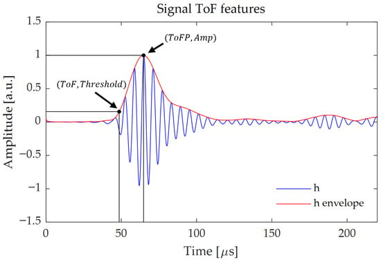
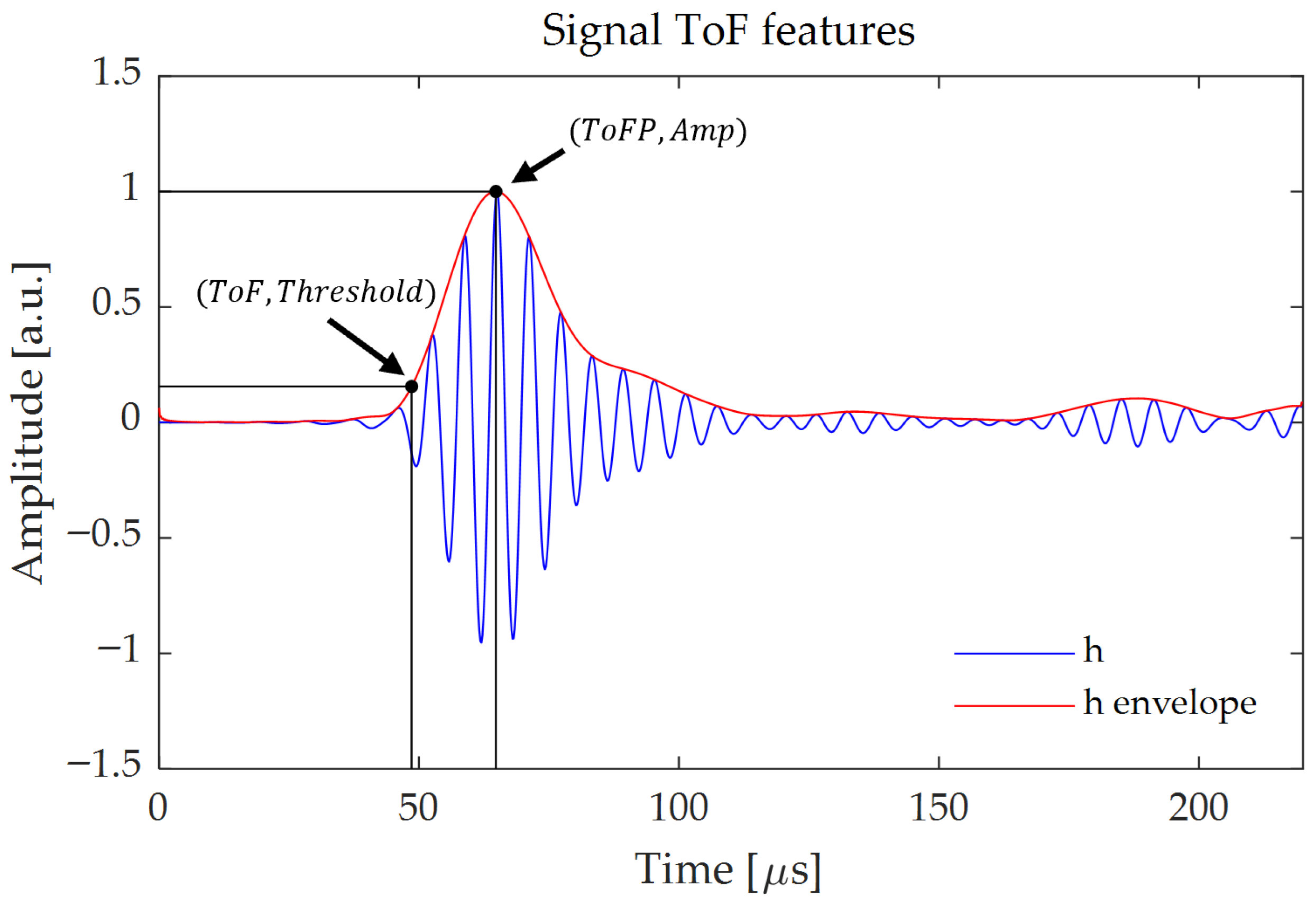
The onset time-of-flight mimics the “standard” $ToF$ measured in the UPV test, but here it is extracted from the output of the PuC procedure. $ToF$ is defined as the first value of time that the signal $h\left(t\right)$ exceeds a certain amplitude threshold of the peak amplitude ($Amp$) of the signal envelope; see Figure 3. In theory, to closer estimate the true $ToF$ value, low threshold levels should be chosen, though the optimal value depends on the amount of noise present in the signal. We therefore calculated the $ToF$ for various threshold values and selected the smallest one guaranteeing a $ToF$ trend without abrupt changes of values due to the noise. After testing the six samples, we chose a threshold equal to $20\%$ of $Amp$. As an alternative strategy to avoid the threshold selection, a $ToF$ estimator based on the Akaike criterion is defined in [35], which detects the onset of the signal by analyzing the trend of the signal variance with time. In the following, we name this feature $To{F}^{AIC}$ and we compare it with the $ToF$ extracted at different threshold values. $To{F}^{AIC}$ is defined as follows, where $T_h$ is the time interval of interest, i.e., the time duration of the reconstructed $\left\{h_n\left(t\right)\right\}$ due to the sample thickness and the estimated sound velocity:

$$To{F}^{AIC}=arg\underset{\tau \in (0,T_h)}{min}\left[\tau \log \left(\mathrm{var}\right\{h\left(t\right):t\in [0,\tau ]\left\}\right)+(T_h-\tau )\log \left(\mathrm{var}\right\{h\left(t\right):t\in [\tau ,T_h]\left\}\right)\right].$$

(6)

Figure 3. Graphical representation of the $ToF$, $ToFP$ and $Amp$ features extracted from the envelope of a generic $h\left(t\right)$ signal (red).

Note that for both definitions, $h\left(t\right)$ can be any of the $\left\{h_n\left(t\right)\right\}$ reconstructed with the $ESS-PuC$ procedure. Differently from the previous NL-UT analysis, we can therefore extract and evaluate also a $ToF$ related to the nonlinear response. This could be a useful indicator for hysteresis characterization as the opening and closing of cracks during cycling load, as well as frictional Sliding of aggregate-mortar disbonding, should impact more the nonlinear ToF than the linear one.

2.2.2. Peak Time-of-Flight—$ToFP$ and Peak Amplitude—$Amp$

The peak time-of-flight and the peak amplitude are defined as the time at which the $h\left(t\right)$ signal reaches its envelope peak, and the value of the peak, respectively; see Figure 3. The envelope of $h\left(n\right)$ is calculated by taking the absolute value of the analytic signal ${\zeta }_h\left(t\right)$ of $h\left(t\right)$ defined as

$${\zeta }_h\left(t\right)=h\left(t\right)+\mathcal{H}\left\{h\left(t\right)\right\}$$

(7)

where $\mathcal{H}\{·\}$ is the Hilbert transform.

2.2.3. Energy Time-of-Flight - $ToFE$, Energy Rate—$\nu E$ and Total Energy—$maxE$

These features are based on reference [12] and are derived by the cumulative energy $E\left(t\right)$ of signal $h\left(t\right)$:

$$E\left(t\right)={\int }_0^t{h}^2\left(\tau \right)d\tau$$

(8)

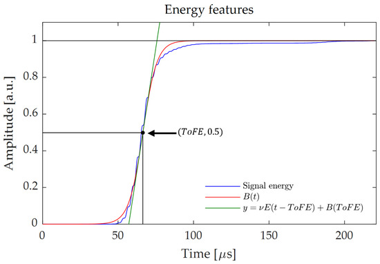
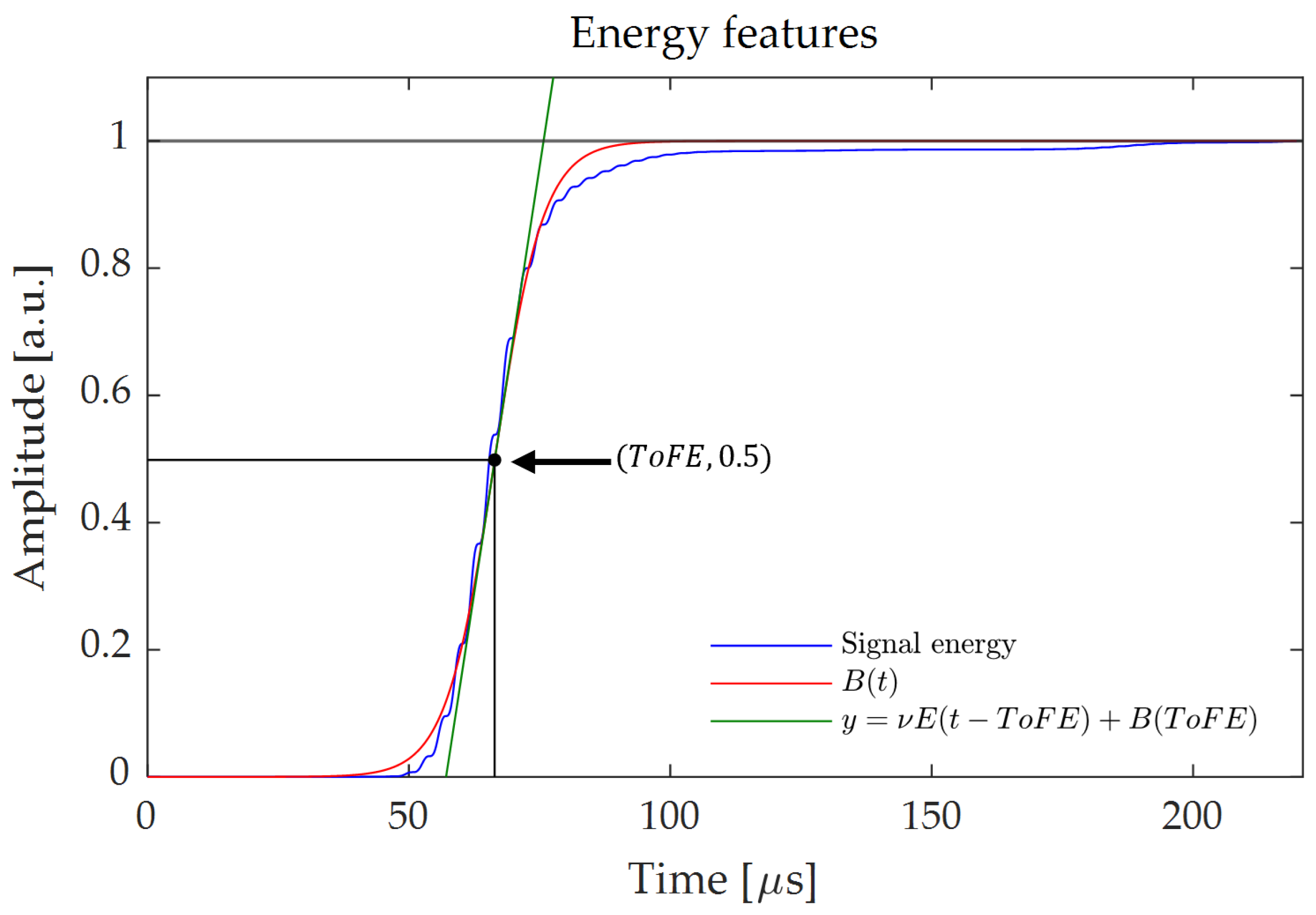
$maxE$ is the last value of $E(t=T_h)$ where $T_h$ is the time interval of interest; see Equation (6). In particular, in [12] a feature extraction algorithm was developed, based on the fitting of the cumulative curves retrieved for each scanning point. A Boltzmann function $B\left(t\right)$ having two free parameters $\nu E$ and $ToFE$ was chosen for the fitting, and was of the form

$$B\left(t\right)={\displaystyle \frac{1}{1+e^{-\nu E·(t-ToFE)}}}$$

(9)

The exploited nonlinear curve fitting algorithm searched for the optimal values of the parameters $\nu E$ and $ToFE$; see Figure 4. In this way, a fitted curve was obtained for each retrieved cumulative energy plot.

Figure 4. This figure shows all the features extracted from the signal energy. All features are derived from the Boltzmann fitting curve (red) of the normalized energy (blue).

We also compared the $ToFE$ feature with the time at which $E\left(t\right)$ crosses the threshold value of $0.5maxE$, and the two values were always very close. As with the fit we also extracted $\nu E$, which can have hidden correlations with some sample properties; we preferred to maintain the current definition for $ToFE$.

2.3. Energy Distortion—ED

In analogy with the concepts of Harmonic Distortion, Total Harmonic Distortion and Distortion Factor, we defined a figure of merit, called Energy Distortion (ED), as follows:

$$E{D}_n={\displaystyle \frac{max{E}_n}{max{E}_1+max{E}_n}}\mathrm{with}n>1$$

(10)

that can be calculated for any harmonics. In particular, we focus on $n=2$, as the 2nd harmonic is usually the most significant term among all the harmonics for NL-UT, so we use equivalently $ED$ or $E{D}_2$. We also report $ED$ in logarithmic form: $E{D}_{\mathrm{dB}}=10{log}_{10}\left({\displaystyle \frac{max{E}_2}{max{E}_1+max{E}_2}}\right)$.

$ED$ quantifies the relative increase in the second harmonic energy during the compression test. This parameter provides an effective measure of the relative enhancement of the second harmonic component, offering valuable insights into the material’s nonlinear response. $ED$ can serve as an early detection tool for stressed concrete, as variations in its value may indicate changes in the material’s microstructural integrity before visible damage occurs.

2.4. Experimental Setup

The experimental tests were performed on several concrete cubes ($150\times 150\times 150$ [mm³]) to optimize the technique. Then, six samples representing three mix designs were selected to cover different compressive strengths. CEM II/A-LL 42.5 N cement was used; siliceous fine aggregate (D_max = 4 mm) and siliceous coarse aggregate (D_max = 16 mm) were employed with constant S/CA weight ratio = 1.04. A Sika super-plasticizer (SPA) tuned consistency (S4). Tap water (W) at $20\pm 2$ °C was used. Cubes were demolded after 24 h and cured for 28 days at $20\pm 2$ °C. The compositions and specimen mapping are reported in Table 1.

Table 1. Mixture compositions and specimen mapping. Ratios by weight: A/C stands for Aggregate/Cement; W/C stands for Water/Cement, SPA (super-plasticizer) is expressed as % of cement. RCM28: 28-day compressive strength; CoV in parentheses.

Mixture	A/C	W/C	SPA [%]	Consistency	RCM28 [MPa] (CoV)	Samples
MIX_1	6.40	0.60	0.28	S4	35.0 (0.05%)	2, 3
MIX_2	5.25	0.50	0.43	S4	44.0 (4.75%)	1, 4, 5
MIX_3	4.55	0.41	0.60	S4	55.5 (4.1%)	6

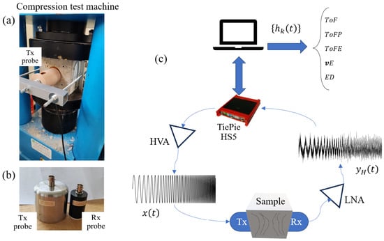
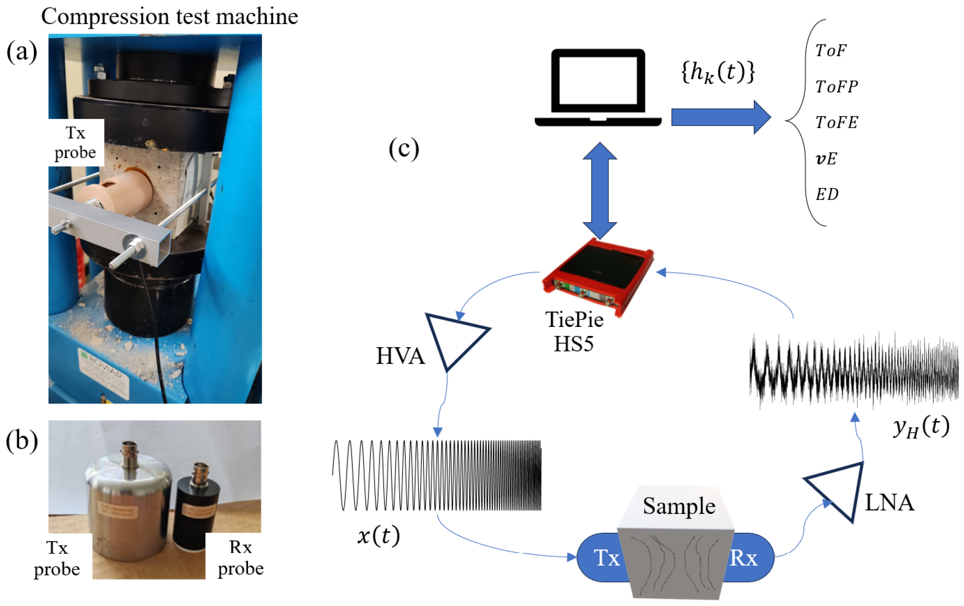
Compressive tests were carried out in accordance with UNI EN 12390-4 using a Matest C070 hydraulic press (Matest SpA, Treviolo, Italy), while ultrasonic measurements were simultaneously taken every ten seconds throughout the entire duration of the test. These measurements were acquired in the direction transverse to the applied load. The acquisition system consisted of two different broadband ultrasonic probes from EofE Ultrasonics Ltd. (Goyang-si, Republic of Korea) operating in transmission configuration; see Figure 5. The two probes are centered at different frequencies, the Tx at 160 kHz and Rx at 350 kHz. Thanks to the large bandwidth, the Rx covers both the Tx excited bandwidth and the relative harmonics, up to the third and part of the fourth.

Figure 5. (a) Matest C070 compression test machine and detail of the mechanical holder that ensures a stable coupling between the Tx and Rx (here not visible) transducers and the SUT. (b) EofE Ultrasonics Ltd. ultrasonic probes used in the experiment: the Tx is centered at $160$ kHz with an active element of $1\frac{3}{4}$ inches, the Rx transducer is centered at $350$ kHz with an active element of 1 inch. (c) Schematic of the measurement procedure.

A digital oscilloscope Handyscope HS5 from TiePie engineering (Sneek, The Netherlands) was used for both signal generation and acquisition. Additionally, a high-voltage amplifier (HVA) WMA-300 from Falco Systems (Hilversum, The Netherlands) was employed to drive the Tx transducer to ensure enough input energy to induce nonlinear phenomena. Figure 5 shows the scheme of the entire system.

Regarding the generated and acquired signals, the exponential chirp exciting the Tx transducer spanned from $f_1={\displaystyle \frac{2f_c}{3}}=110$ kHz to $f_2={\displaystyle \frac{4f_c}{3}}=220$ kHz. For all the tests, the chirp duration was $\approx 2.2$ ms, while the acquisition of the Rx signal lasted for the excitation time plus further $0.2$ ms, corresponding to the duration of the reconstructed $\left\{h_n\left(t\right)\right\}$. For instance, assuming a ultrasonic velocity of 4500 m/s, $0.2$ ms correspond to 90 cm of travel path, quite larger than the samples’ thickness. The sampling rate for both generation and acquisition was equal to 5 MSa/s. Please note that the exact chirp duration is calculated for assuring specific alignment of phase values of the exponential chirp; further it can be shortened/extended to reduce/increase the SNR after the PuC. The value here adopted was a trade-off between SNR and computational costs. Moreover, during the compression, a measure was collected every ten seconds, and for each measure twenty repetitions of the chirp generation and signal recording were acquired to perform averages to further improve the SNR. Note that the SNR could be improved by extending the duration of the chirp and doing just one measurement, but we opted for collecting several repetitions to have the possibility to filter out possible acquisitions affected by external anomalous coupled electrical noise or by errors in synchronization. Further, to optimize the SNR gain, we firstly performed the PuC for each repetition, then we aligned the various $h_n\left(t\right)$ before the averaging by also measuring the excitation signal that drives the HVA. In this way, we can apply sub-sampling shift to each repetition to counterbalance the jitter of the HS5 internal trigger. As will be shown later, the averaging is fundamental to achieve enough SNR on the reconstructed nonlinear impulse responses.

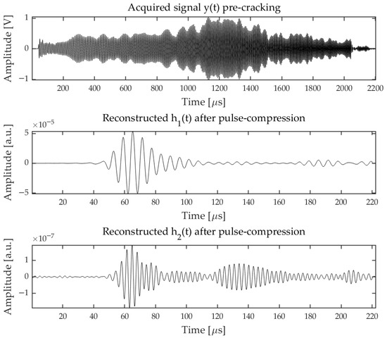
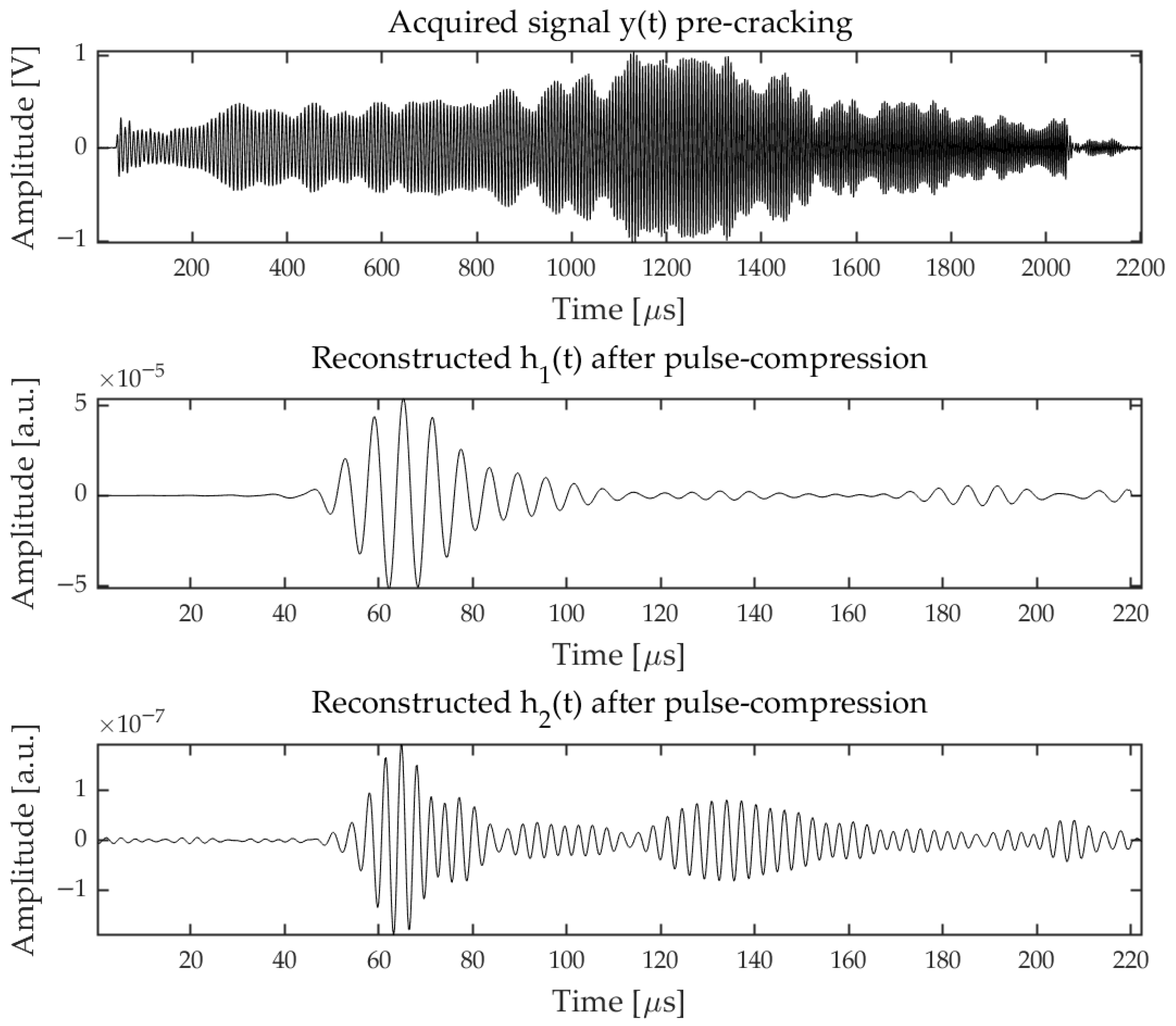
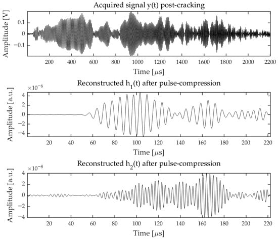
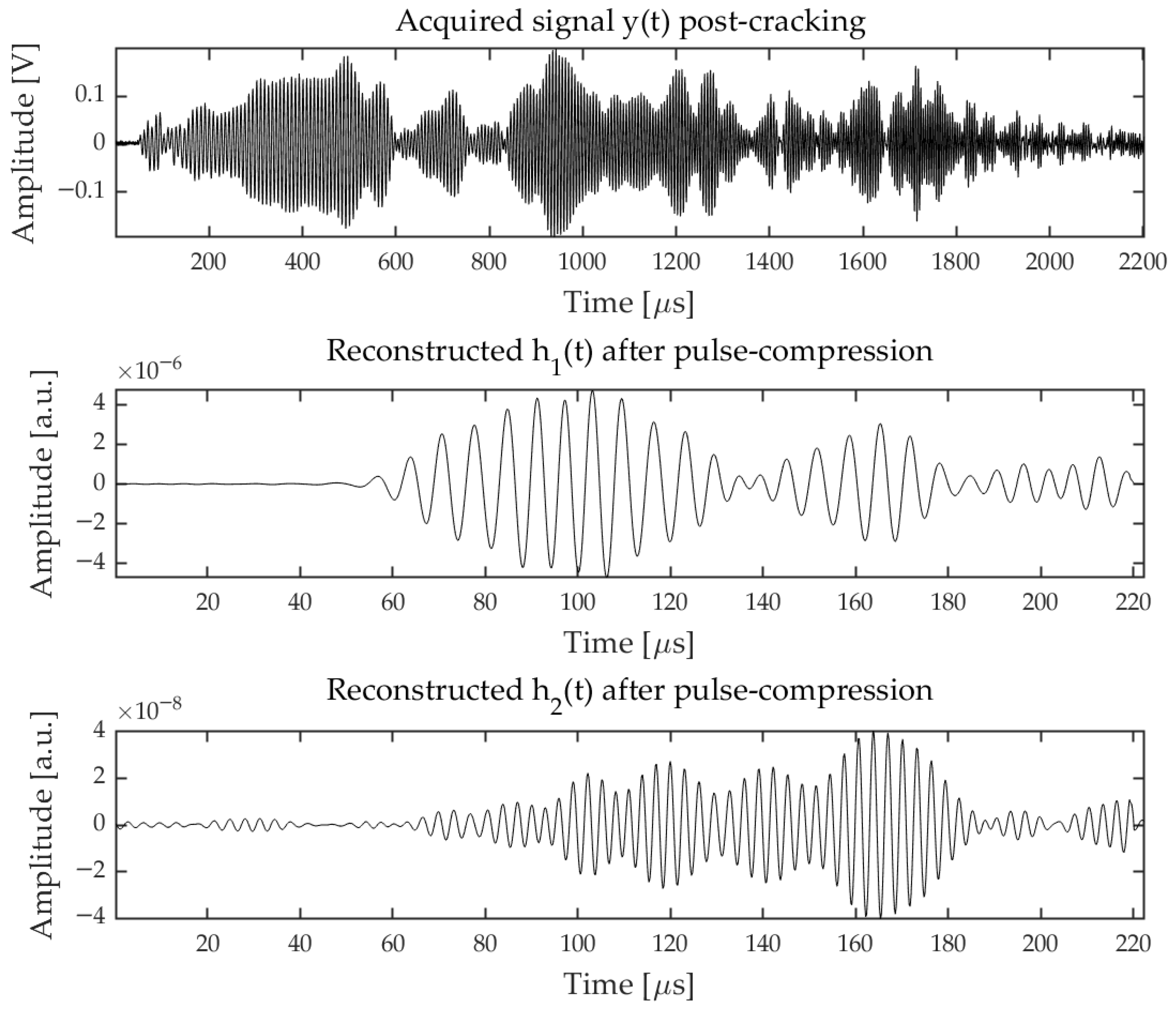
Figure 6 and Figure 7 report some examples of acquired signals $y\left(t\right)$ and relative $h_1\left(t\right)$ and $h_2\left(t\right)$ after the averaging. The two measurements were done on the same sample at the beginning of the compression test (pre-cracking) and after the start of cracking (post-cracking). It can be seen that the maximum amplitude and energy of $y\left(t\right)$ decrease significantly (a factor ≈10 and ≈100 respectively), and a similar amplitude attenuation factor was found as expected on $Am{p}_1$ feature pre- and post-cracking, i.e., on the maximum amplitude of $h_1\left(t\right)$. At the same time $h_1\left(t\right)$, post-cracking is evidently shifted toward higher ToF values, and the energy spreads more in time than in the pre-cracking condition. Interestingly, $h_2\left(t\right)$ exhibits a similar behavior, and $Am{p}_2$ decreases as $Am{p}_1$, while in the case of an intrinsic nonlinearity of the measurement system, $Am{p}_2$ should scale $\propto {\left(Am{p}_1\right)}^2$. We interpret this fact by assuming that in post-cracking conditions the 2nd harmonic generation is enhanced compared to that in pre-cracking conditions.

Figure 6. Examples of acquired signals $y\left(t\right)$ and resulting $h_1\left(t\right)$ and $h_2\left(t\right)$ collected on the same sample in pre-cracking conditions. Note the time scale (x axis) is expressed in microseconds.

Figure 7. Examples of acquired signals $y\left(t\right)$ and resulting $h_1\left(t\right)$ and $h_2\left(t\right)$ collected on the same sample in post-cracking conditions. Note the time scale (x axis) is expressed in microseconds.

3. Results

This section presents the experimental results obtained from the ultrasonic tests performed on concrete specimens subjected to compression loading. The results are structured to highlight the comparison between the linear and nonlinear ultrasonic features defined and analyzed, as well as their effectiveness in detecting structural changes. Firstly, the typical behavior of the various features is discussed, then a comparison between different samples is reported.

Without being exhaustive, for each samples we compared:

• The different time-of-flight features related to the linear response;
• The different time-of-flight features related to 2nd harmonic response;
• The energy features of the linear and 2nd harmonic terms.

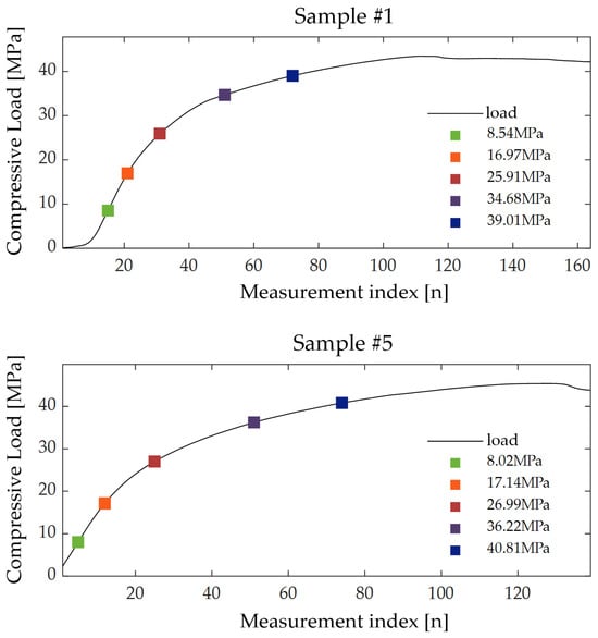
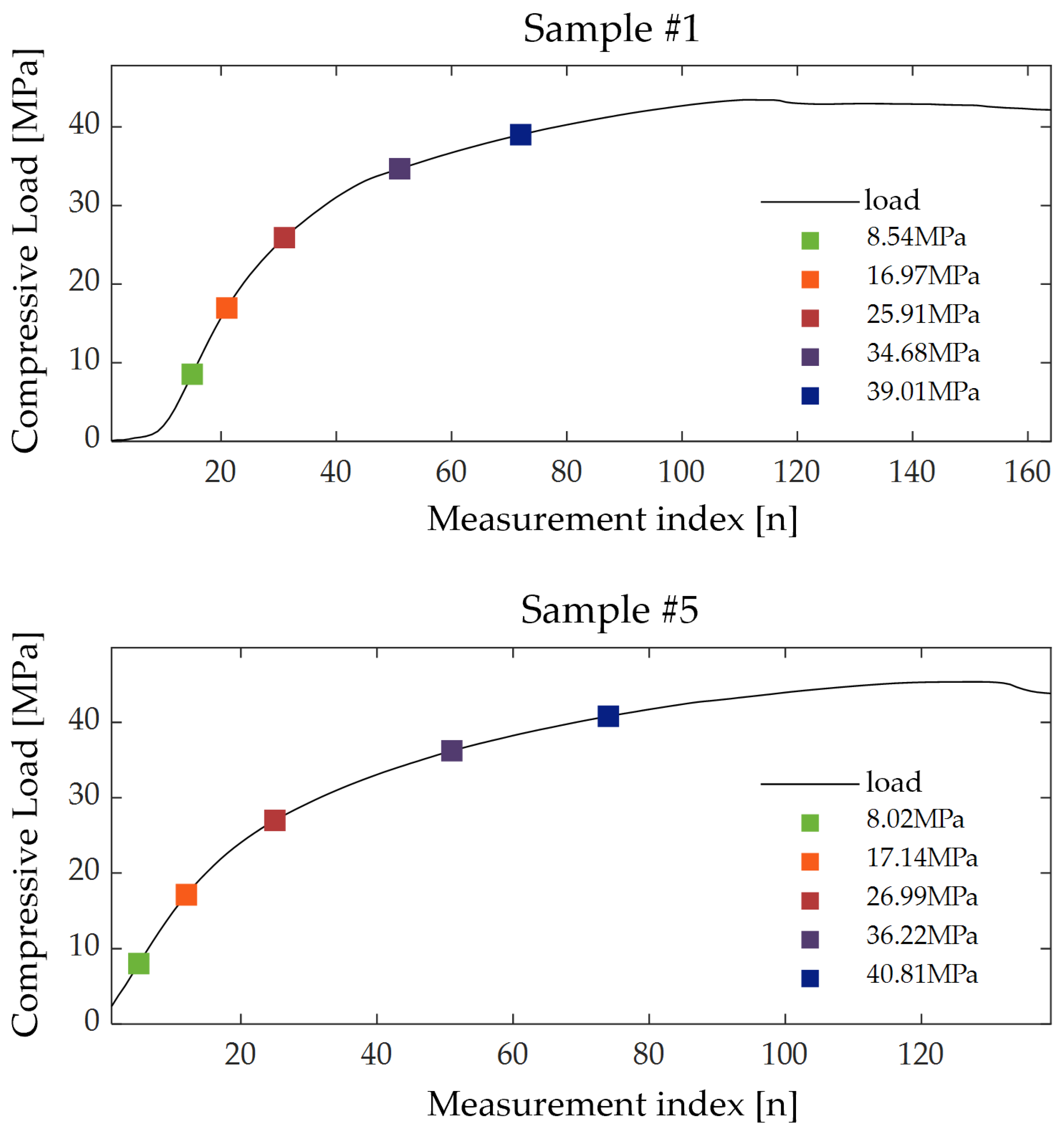
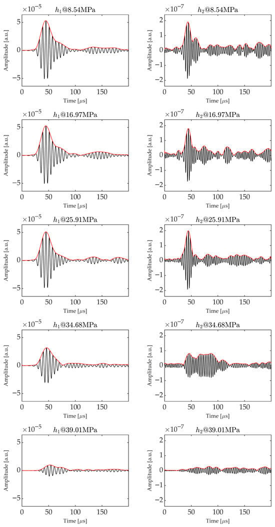
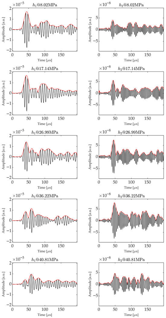
To extend the early comparison reported in Figure 6 and Figure 7, we analyzed the time trends of $h_1\left(t\right)$ and $h_2\left(t\right)$ at different compression values during the tests. Precisely, we selected specific points along the compression curve as shown in Figure 8 for sample $\#1$ and $\#5$, and for these points we plotted in Figure 9 and Figure 10 the corresponding $h_1\left(t\right)$’s and $h_2\left(t\right)$’s.

Figure 8. Trend of the compressive load with respect the measurement index. Colored squares indicate selected points for sample $\#1$, and sample $\#5$ is used in Figure 9, Figure 10 and Figure 11.

Figure 9. Time trends of $h_1\left(t\right)$ and $h_2\left(t\right)$ at the different values of load reported in Figure 8 for sample $\#1$. The increasing attenuation and the onset of secondary peaks for both $h_1\left(t\right)$ and $h_2\left(t\right)$ are visible as long as the compression increases.

Figure 10. Time trends of $h_1\left(t\right)$ and $h_2\left(t\right)$ at the different values of load reported in Figure 8 for sample $\#5$. It can be seen how in this case the secondary peak becomes larger than the first one for $h_1\left(t\right)$, while the general behavior in terms of attenuation is maintained for sample $\#5$ as for $\#1$.

Although every sample can exhibit some peculiar trends, a common behavior is evident for all of them. Specifically, as the compression increases, $h_1\left(t\right)$ exhibits an attenuation, which aligns with expectations, as internal fractures are created. Besides the increased attenuation, the overall signal time-shape changes: the barycenter of the signal envelope shifts toward the right (larger times) as the compression increases, and some late local peaks can emerge differently from the first one in time, suggesting the presence of different paths for the UT waves. In some cases, these peaks could become larger than the first one, leading to jumps in the $ToFP$ value.

For instance, Figure 10 clearly shows that the first peak in the $h_1\left(t\right)$ envelope—corresponding to the direct path between the Tx and Rx transducers—is initially the most prominent. However, as compression increases, this peak diminishes and eventually becomes smaller than the second peak. This transition results in a sudden increase in the $ToFP$ feature, which can oscillate between two distinct values when the amplitudes of the first and second peaks are nearly equal over a range of compression levels. On the contrary, the $ToF$ feature is less sensitive to such changes in the $h\left(t\right)$ time trend, as it is calculated when the signal amplitude crosses a threshold level, proportional to the maximum envelope amplitude. This aspect could be interpreted as a higher sensitivity of the $ToFP$ feature to the early detection of cracks with respect to $ToF$.

A similar observation can be made for the second harmonic, even if $h_2\left(t\right)$ is, in general, more noisy than $h_1\left(t\right)$. This is reflected in the $To{F}_2$ and $ToF{P}_2$ trends.

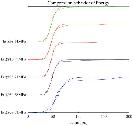
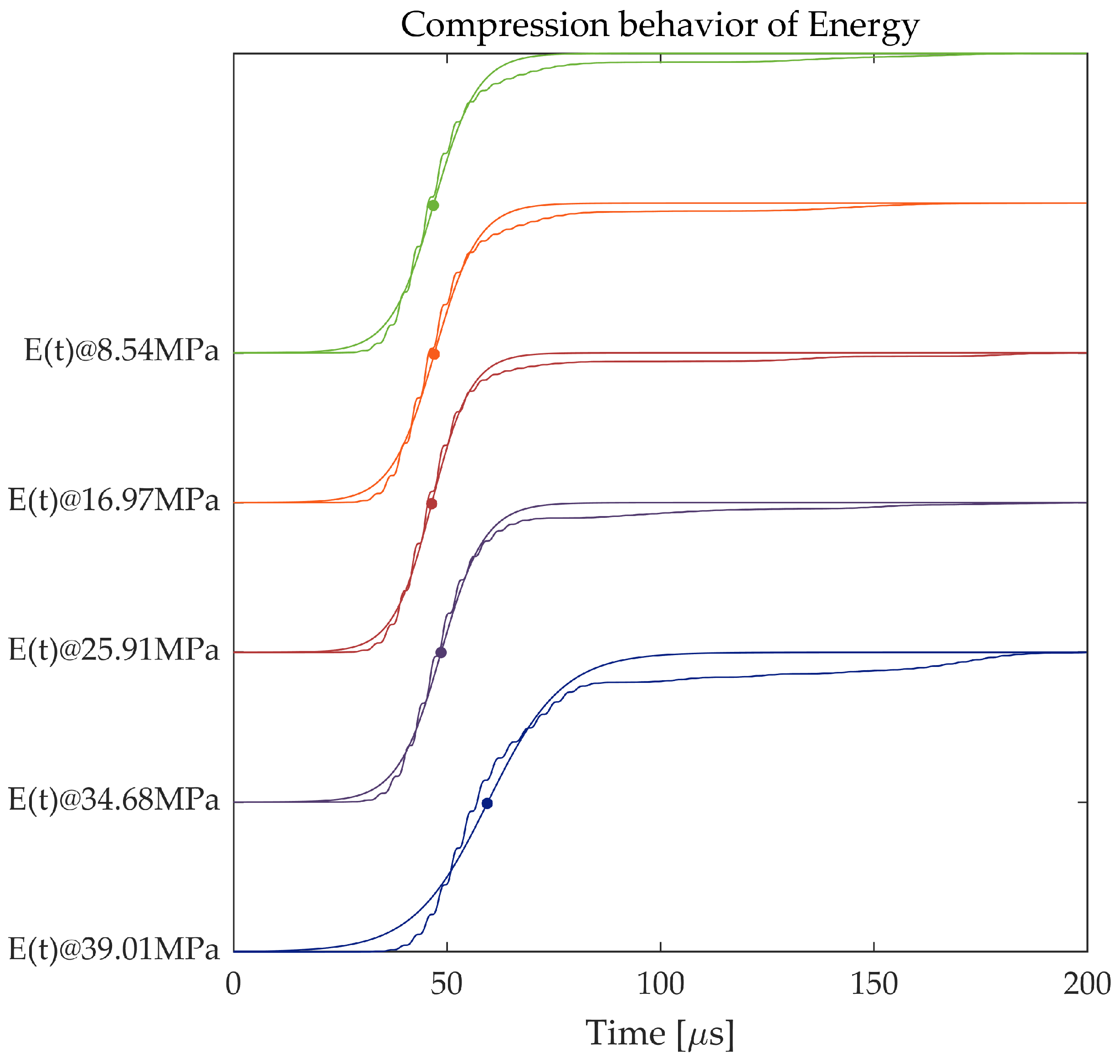
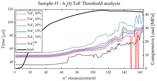
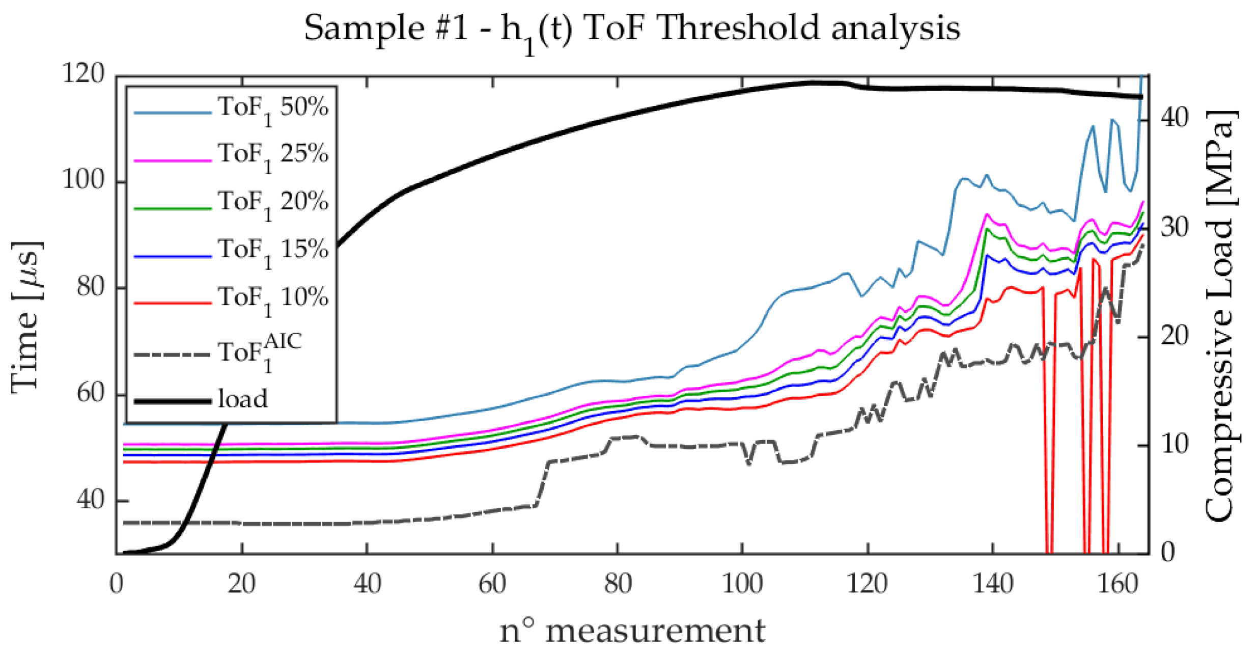
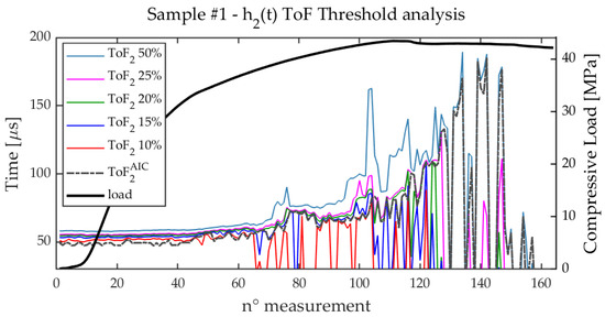
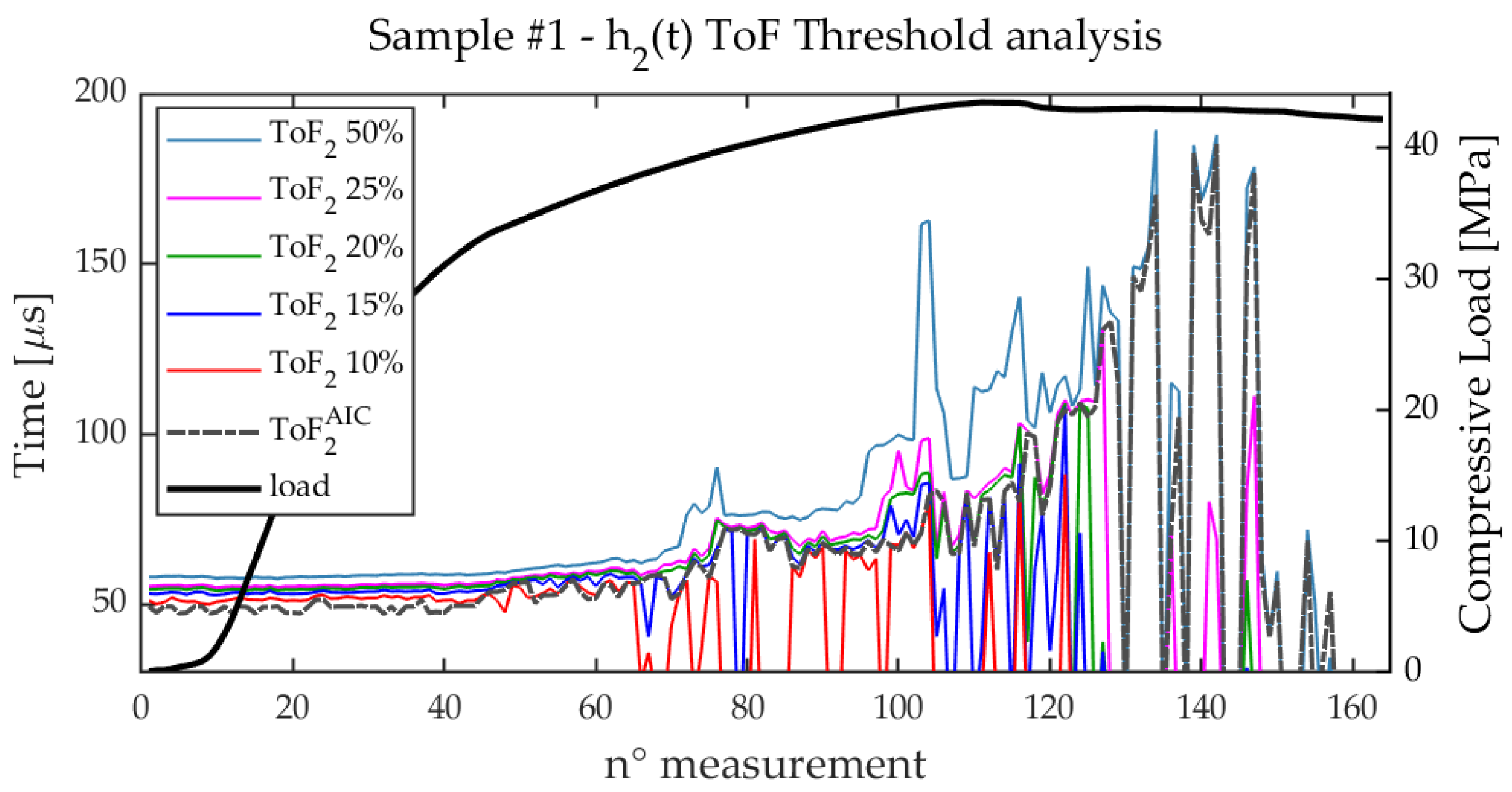
By looking at the cumulative energy plot at different load values, the time-spreading of the $h\left(t\right)$’s due to the presence of multiple transmission paths reflect on the $E\left(t\right)$’s trends. By focusing on $E_1\left(t\right)$, which has larger SNR than $E_2$, a progressive shift toward the right is observed while the compression strength increases, together with a widening and smoothing of the $E\left(t\right)$ rise. This effect is represented in Figure 11 that plots the $E_1\left(t\right)$ curves corresponding to the compression points reported in Figure 8 for sample $\#1$. This $E\left(t\right)$’ behavior is expected: in the case of a single transmission path, all the energy reaches the RX transducer in a short time interval determined by the duration of the equivalent excitation after pulse-compression. If multiple propagation paths are present, $E\left(t\right)$ increases more slowly and may exhibit the step-like features associated with the arrival of different paths. In this paper, we compared the feature $ToFE$ extracted from fitting $E\left(t\right)$, and the $ToF$ and $ToFP$ features directly extracted from $h\left(t\right)$. Before doing this, Figure 12 and Figure 13 report the analysis of $To{F}_1$ and $To{F}_2$ at different threshold values, compared with $To{F}^{AIC}$ for sample $\#1$. A similar analysis was done for all the samples. While $To{F}_1$ is correctly estimated in most of the cases, just showing some failures for low threshold values and for post-cracking conditions, in the case of $To{F}_2$, due the lower SNR, the choice of the threshold is more critical, and it could happen that $ToF$ is not correctly estimated neither for $To{F}^{AIC}$, especially after cracking. However, for all the cases analyzed, a threshold of $20\%$ of $Amp$ ensures a very similar trend for $To{F}_2$ and $To{F}_2^{AIC}$; for this reason, henceforth we used this threshold value for all the samples and for both the $To{F}_1$ and $To{F}_2$ estimates. In general, we noticed that $ToF$ is more smooth than $To{F}^{AIC}$.

Figure 11. The figure shows the energies and the related fitting curves $B\left(t\right)$ at different compression points.

Figure 12. The figure illustrates the evolution of $To{F}_1$ during the measurements for different values of the threshold. The dot-dashed curve represents the $To{F}_1^{AIC}$ calculated with the Akaike Information Criterion, while the thick black solid line depicts the compression load curve with the y-axis on the right.

Figure 13. The figure illustrates the evolution of $To{F}_2$ during the measurements for different values of the threshold. The dot-dashed curve represents the $To{F}_1^{AIC}$ calculated with the Akaike Information Criterion, while the thick black solid line depicts the compression load curve with the y-axis on the right.

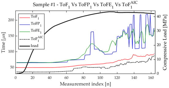
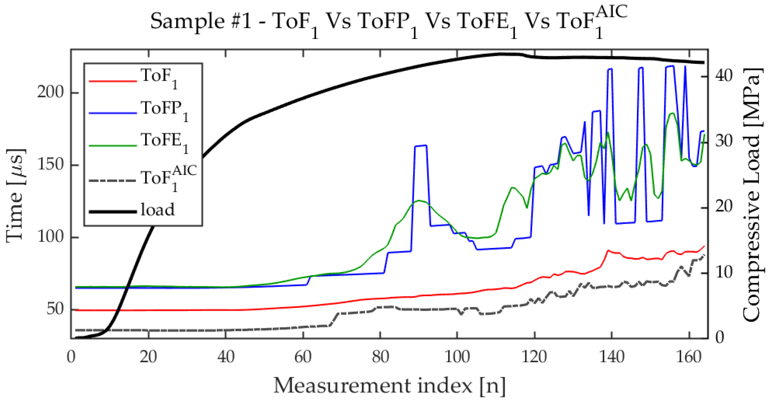
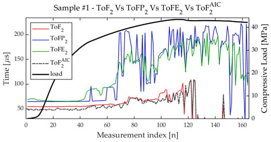
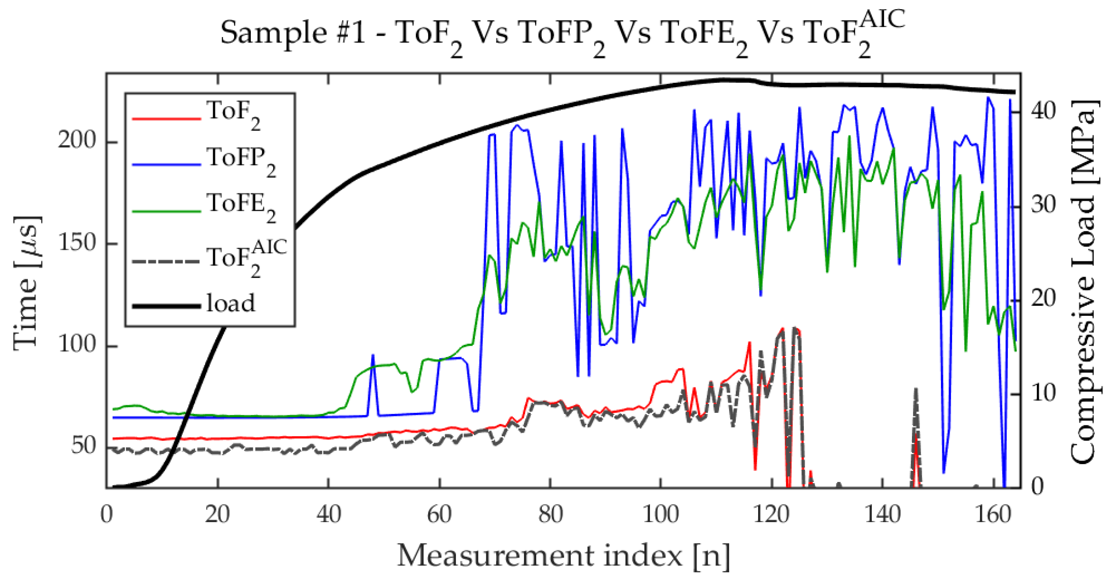
Once having optimized the threshold, we compared $ToF$, $ToFP$ and $ToFE$. Figure 14 and Figure 15 illustrate this comparison for sample $\#1$, starting from $h_1\left(t\right)$ and $h_2\left(t\right)$ respectively. For the linear response, both $ToF{P}_1$ and $ToF{E}_1$ show a significant increase in their values earlier than $To{F}_1$ and $To{F}_1^{AIC}$. $ToF{P}_1$ increases with larger steps, while $ToF{E}_1$ shows a smoother trend and an even earlier onset of the rising. For the second harmonic, the behavior is similar even if the signals are nosier than for the linear response and both $To{F}_2$ and $To{F}_2^{AIC}$ are not properly estimated after a certain level of cracking. Further, $ToF{P}_2$ is very oscillating. On the other hand, $ToF{E}_2$ exhibits enough SNR, and a significant increase starts even earlier than the $ToF{E}_1$; see Figure 15.

Figure 14. The figure illustrates the evolution of $To{F}_1$ (red), $ToF{P}_1$ (blue), and $ToF{E}_1$ (green) during the measurements. The compression curve is shown in black and with the y-axis on the right.

Figure 15. The evolution of $To{F}_2$ (red), $ToF{P}_1$ (blue), and $ToF{E}_2$ (green) during the measurements. The compression curve is shown in black and with the y-axis on the right.

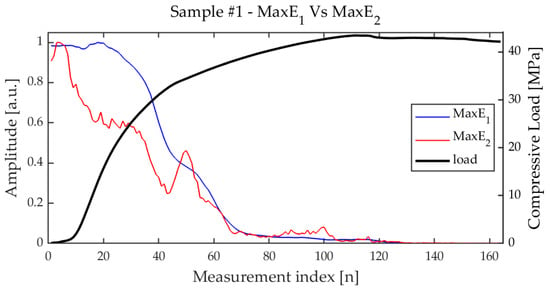
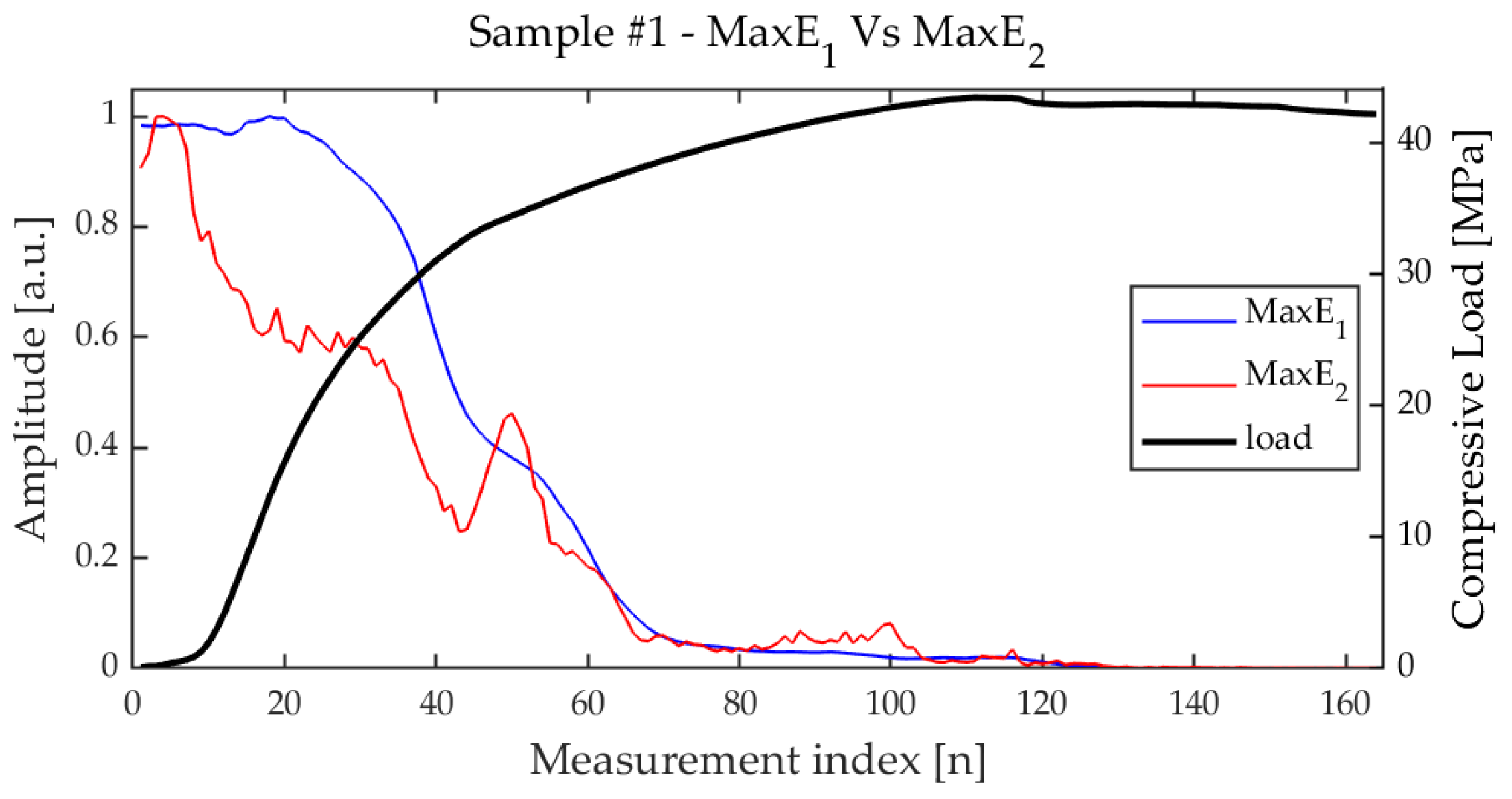
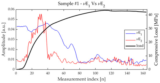
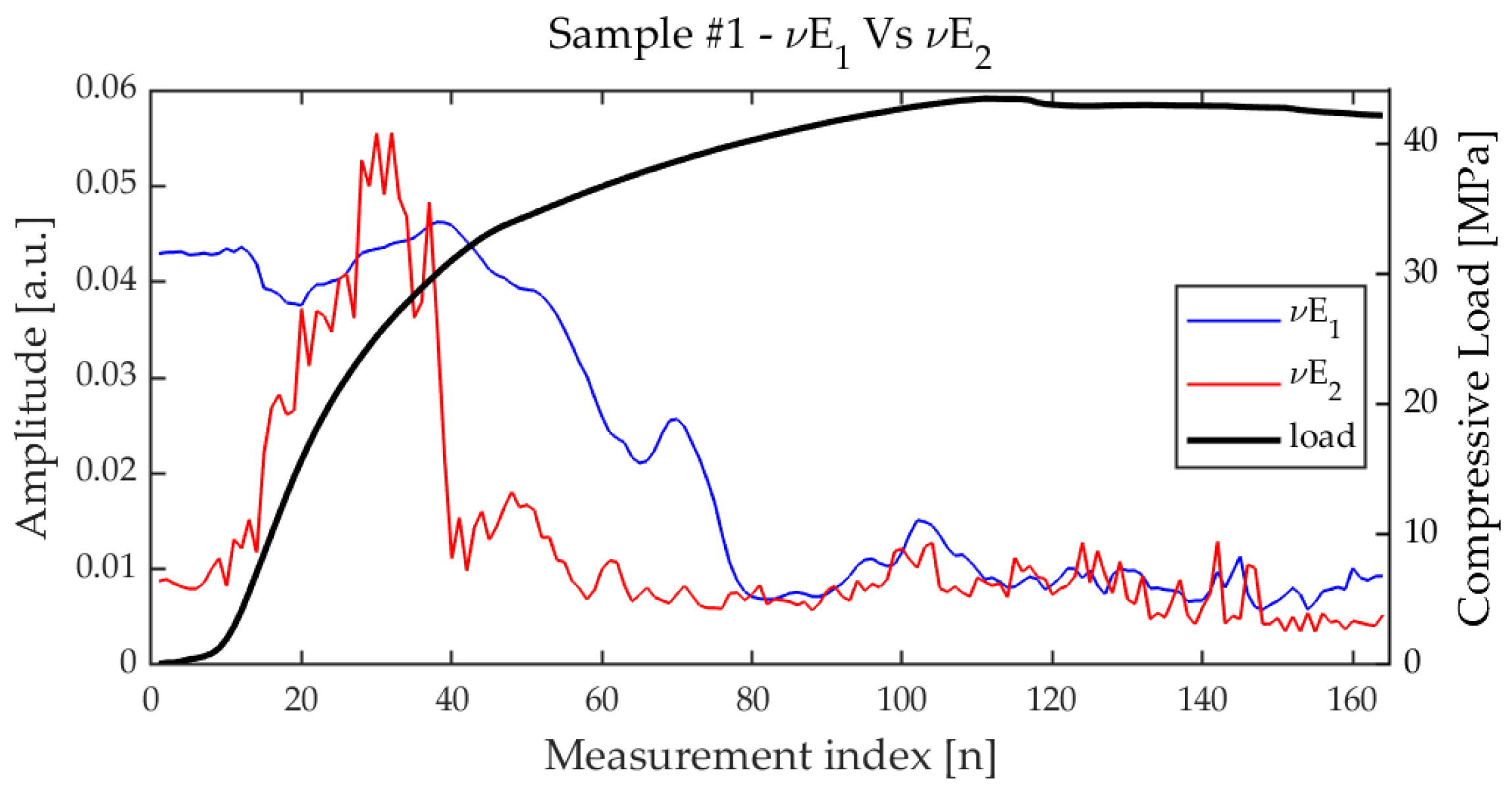
Also $MaxE$ and $\nu E$ were compared for the 1st and 2nd harmonics. For both $Max{E}_1$ and $Max{E}_2$, a decrease was observed as long as the load increased (see Figure 16); on the other hand, while $\nu E_1$ trend is similar to that of $MaxE1$, $\nu E_{h_2}$ shows an irregular trend characterized by an initial steep increase, and a late decrease (see Figure 17). As it will be shown in the following subsection, $\nu E$ is quite unpredictable; nonetheless, it could have hidden correlation with the state-of-health of the sample (see [12]), so we analyzed $\nu E_1$ and $\nu E_2$ for all the samples.

Figure 16. Trend of $Max{E}_1$ (blue) and $Max{E}_2$ (red) during the measurements.

Figure 17. Trend of $\nu E_1$ (blue) and $\nu E_2$ (red) during the measurements.

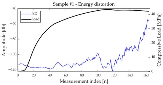
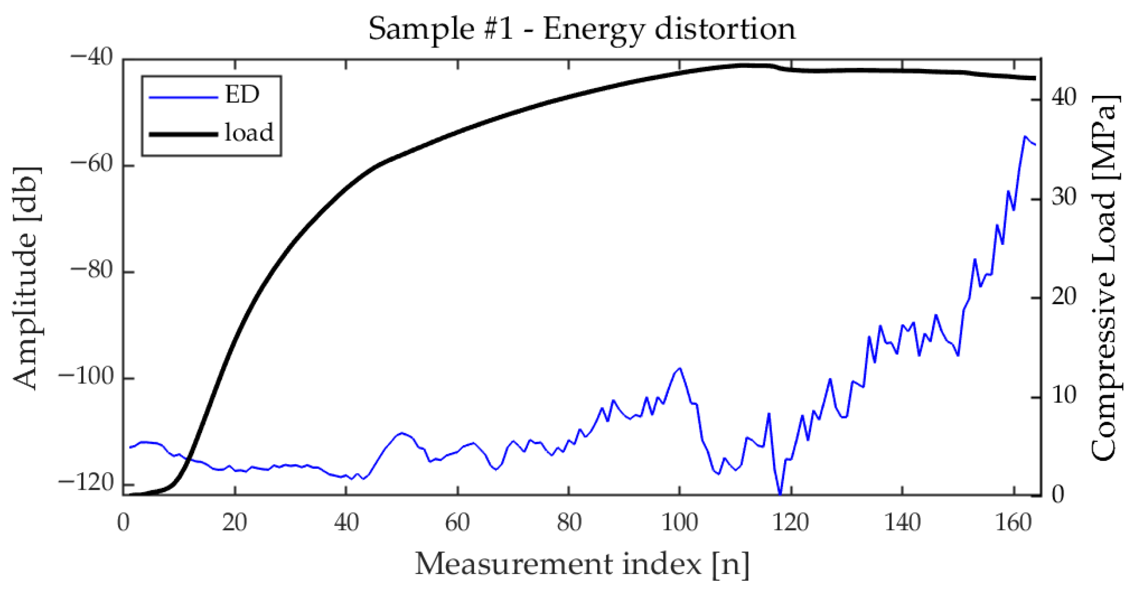
Regarding the $ED$ parameter, as expected, it is quite sensitive to the increase in $Max{E}_2$ and even more to the decrease in $Max{E}_1$, which is significantly larger than $Max{E}_2$, especially at the beginning. $ED$ measures indeed the relative weight of the 2nd harmonic over the energy of the 1st and 2nd harmonics. For this reason, $ED$ could also decrease for short intervals during measurements, even if it tends to increase as the compression increases, as shown in Figure 18.

Figure 18. Trend of the Energy Distortion for sample $\#1$ vs. the measurement index. The corresponding compression load values are also plotted (right y-axis).

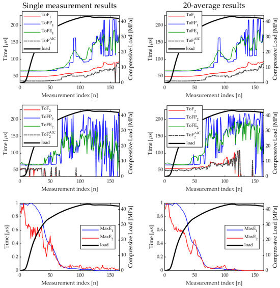
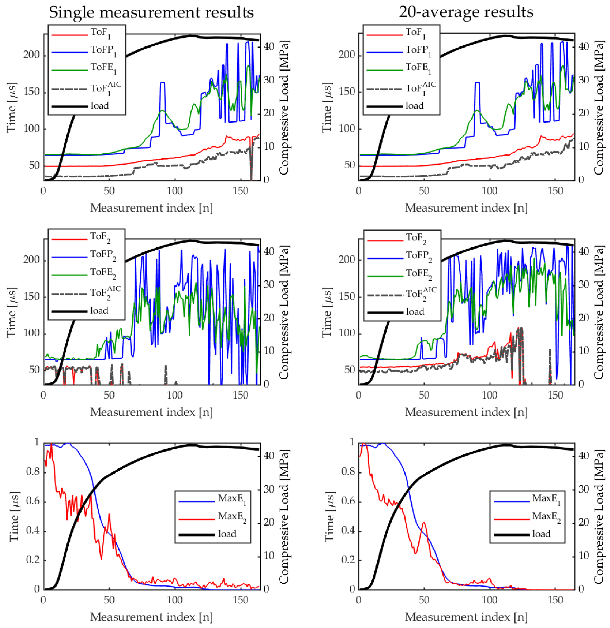
It is worth recalling that the primary goal of this research is to identify a set of robust ultrasonic features capable of yielding consistent and repeatable information for a wide range of concrete characteristics. This information can then be exploited further for evaluating the state of health of the sample/structure under test by defining some health degree index related to the features. The following results are therefore aimed at evaluating the reproducibility of the various extracted features. In particular, the focus is on understanding which of these parameters exhibit a stable behavior across different samples under similar loading conditions, and could serve as reliable indicators for early-stage damage assessment. As a last preliminary analysis before comparing the trends of the features for the various sample selected, we investigated also the effect of the averages on the time-of-flight features and $MaxE$ for $h_1\left(t\right)$ and $h_2\left(t\right)$ for sample $\#1$. The results of the comparison are shown in Figure 19. As previously mentioned, the effect of the averages on features extracted from the linear response is almost negligible; on the contrary, they impact significantly the features extracted from the 2nd harmonic.

Figure 19. Comparison of features extracted from $h_1\left(t\right)$ and $h_2\left(t\right)$ with and without averages.

Comparison

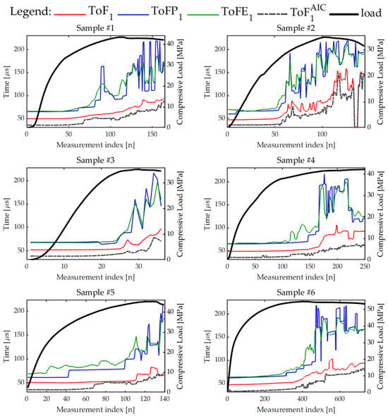
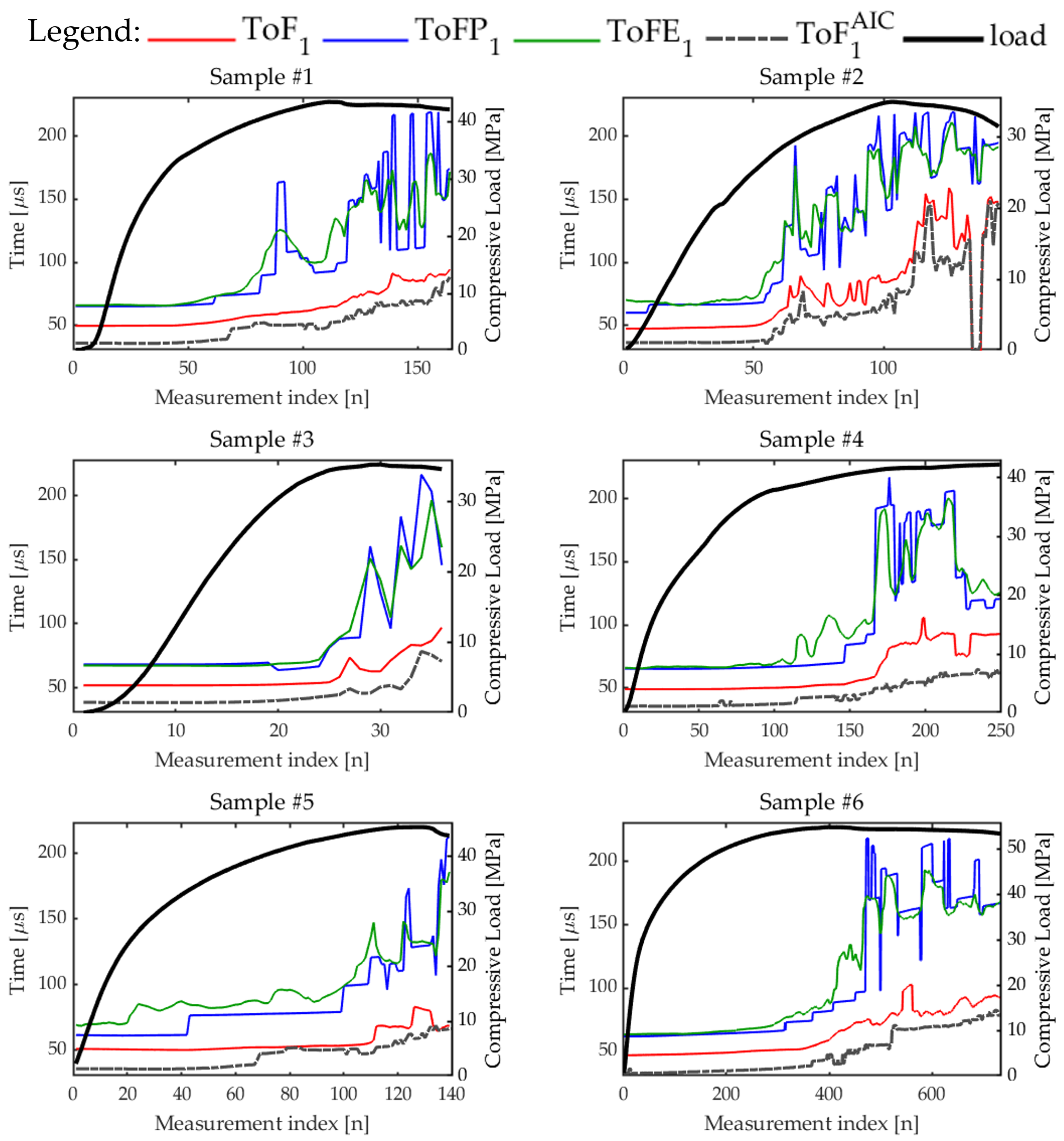
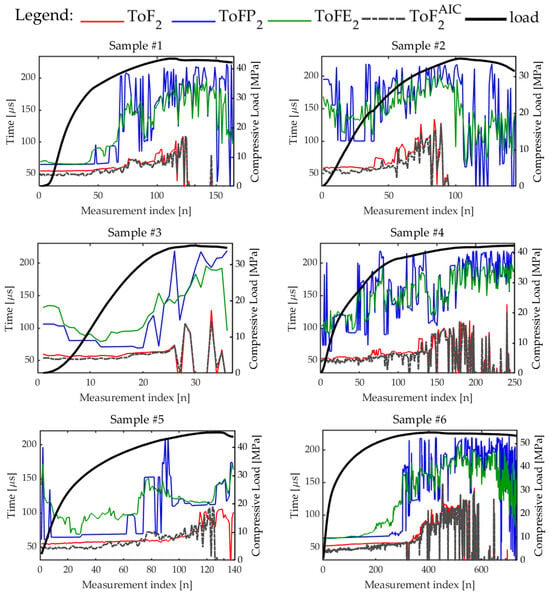
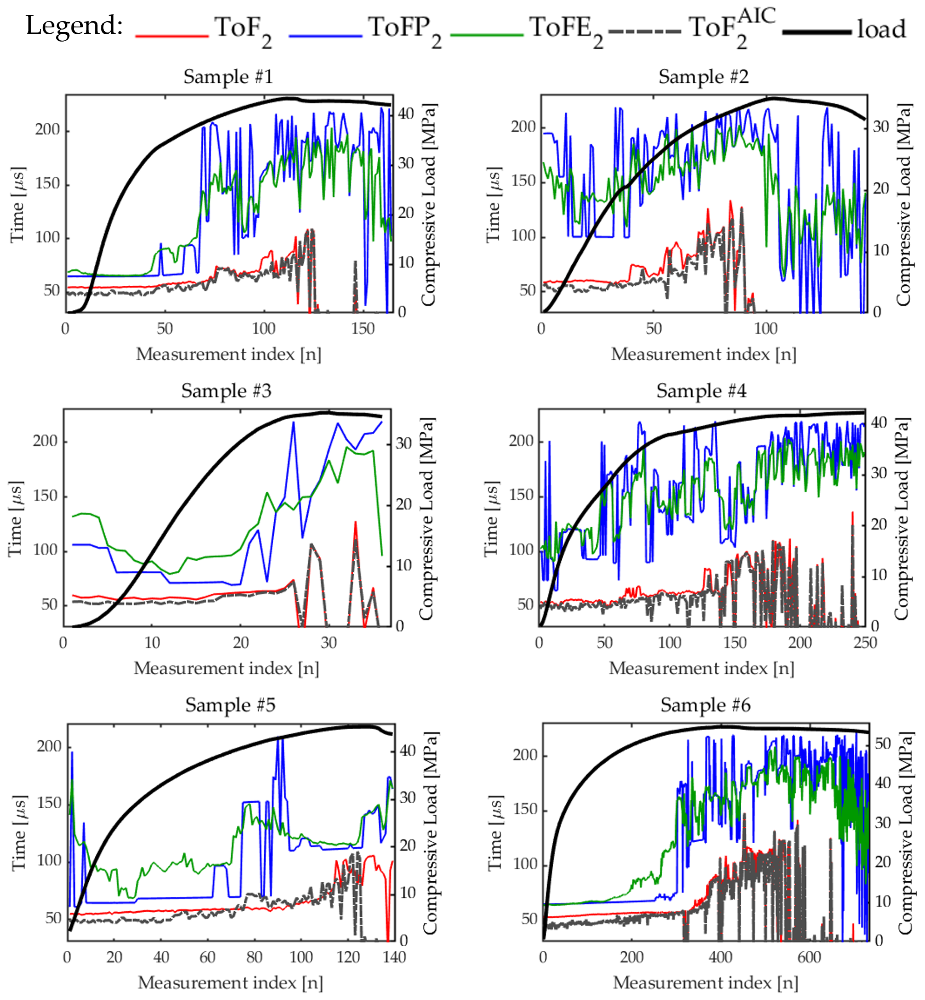
To assess the robustness of the ultrasonic features, tests were carried out on six concrete specimens, characterized by compressive strength ranging between 35 and 55 MPa; see Table 1. The objective was to investigate whether some parameters could consistently track or detect the evolution of damage under compression across different samples. Figure 20 and Figure 21 illustrate the evolution of the $To{F}_1$, $To{F}_1^{AIC}$, $ToF{P}_1$, $ToF{E}_1$, and $To{F}_2$, $To{F}_2^{AIC}$, $To{F}_2$ and $ToF{E}_2$, respectively. Among all the time-of-flight features, $ToFE$ stands out as the least noisy and most regular, even for the case of the 2nd harmonic for which features are significantly noisier in general. Across all tested samples, $ToF{E}_1$ shows a smoother progression and aligns well with the compression trend. In addition, $To{F}_1$, $To{F}_1^{AIC}$ and $ToF{P}_1$ increase with the compression on average, but their rise usually starts a little later than $ToF{E}_1$. $ToF{E}_1$ could thus represent a reliable indicator for monitoring the internal state of concrete under load and to early detect damages. Time-of-flight features from the 2nd harmonic are significantly noisier than the others but similar considerations hold for them. However, it seems that the higher the concrete mechanical resistance, the earlier the rising of all the $ToF$ features with respect to those extracted from the linear term, especially $ToF{E}_2$; see for instance the curves related to samples $\#1$, $\#4$, $\#5$, and $\#6$ in Figure 20 and Figure 21, indicating their potential use as early detectors of cracks opening.

Figure 20. Trends of the time-of-flight features extracted from the linear response for all the samples tested.

Figure 21. Trends of the time-of-flight features extracted from the 2nd harmonic for all the samples tested.

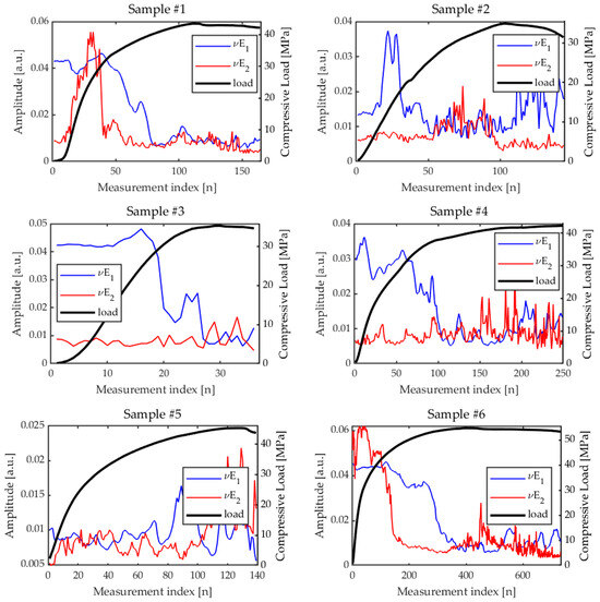
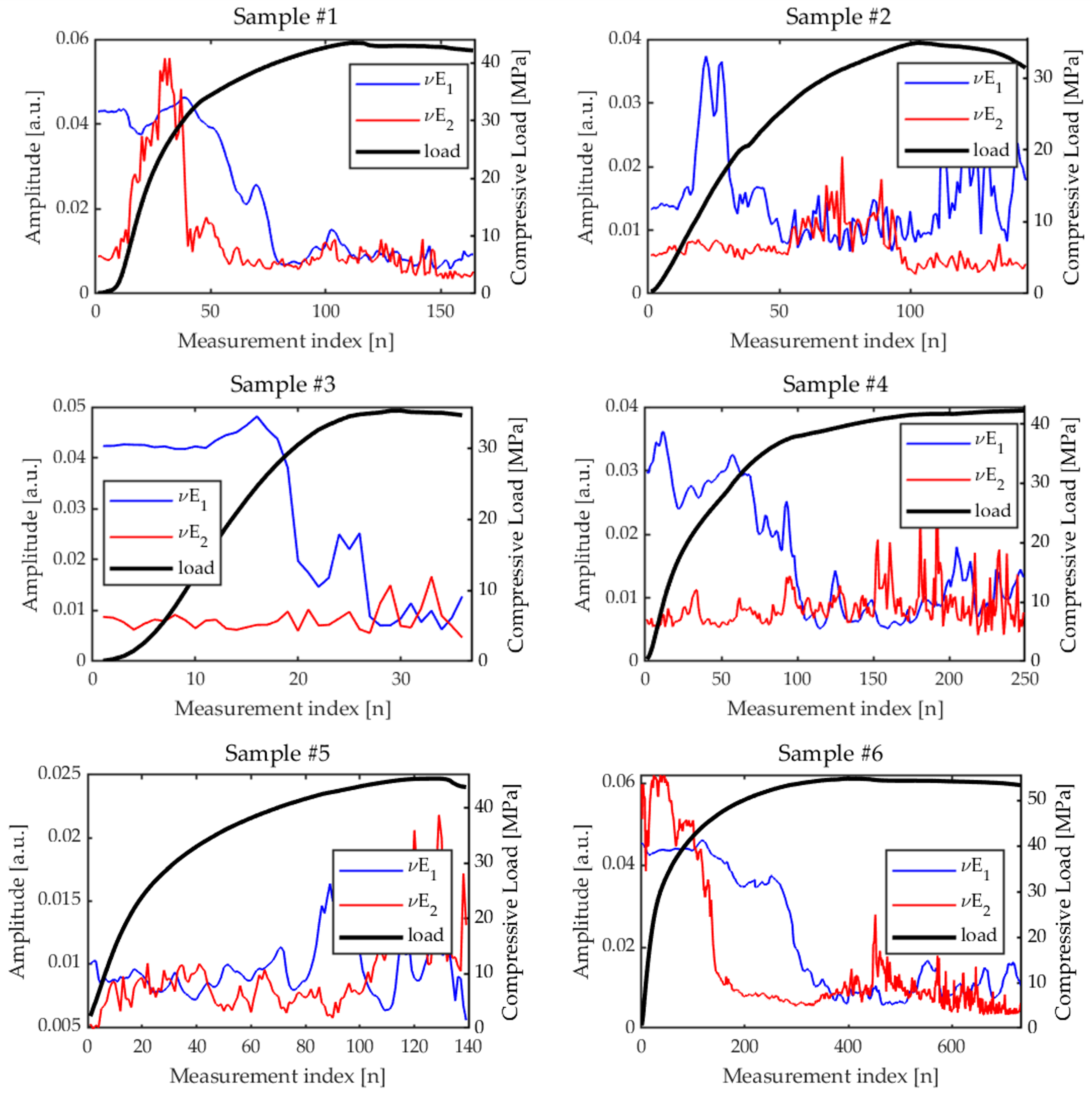
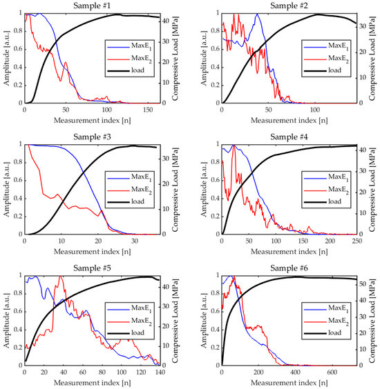
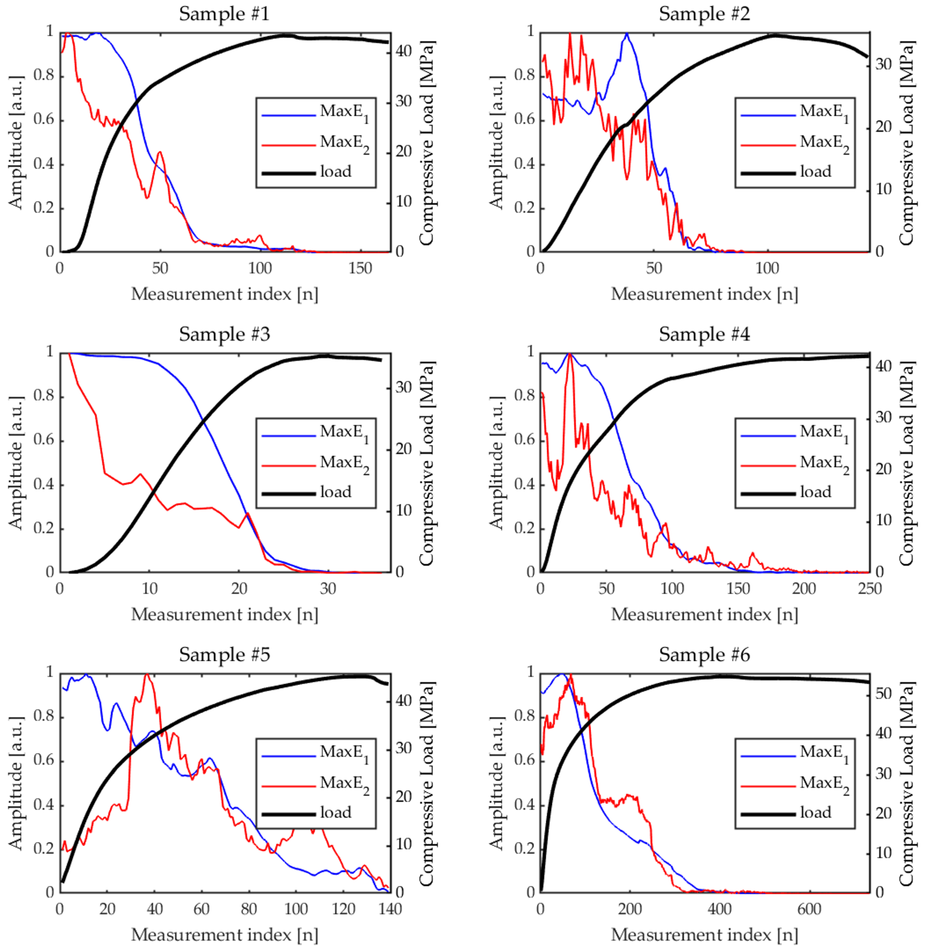
Since $ToFE$’s seem to be robust indicators of the internal state of the concrete, and they are derived through the fitting procedure introduced in [12] and summarized in Section 2.2.3, it is interesting analyzing the other feature extracted by the fit, $\nu E$, which quantifies how spread is the ultrasonic signal in time. The larger $\nu E$ is, the less spread out the ultrasonic energy is over time. Figure 22 shows the evolution during the compression tests of the $\nu E$ parameter for the fundamental ($\nu E_1$) and second harmonic ($\nu E_2$) components. In general, $\nu E$ trends are quite irregular, and not very informative at first glance. Nonetheless, for samples $\#1,3,4,6$, $\nu E_1$ displays similar trends—an initial plateau, then a sudden decrease, and a plateau again—that could be correlated to internal changes. The sudden changes coincide indeed with the rise of $ToFE$, which is not unexpected: as long as the compression increases, cracks open in the sample and multiple paths become available to the ultrasonic beam. Depending on the sample and on the cracks characteristics, as well as their distribution, the ultrasonic signal received by the RX can be more spread in time or not, with the presence of several local peaks of comparable amplitude. In our experimental experience, the less spread the original signal before compression is, the more likely it is that $\nu E_1$, and perhaps $\nu E_2$, will exhibit this sudden decrease. For instance, see Figure 9 and Figure 10: for sample $\#1$, the signal is initially characterized by a main peak, for both the 1st and 2nd harmonics. Then, as compression increases, cracks open, the main peak envelope spreads, and $\nu E_1$ decreases; see Figure 22. On the other hand, sample $\#5$ presents multiple peaks since the beginning, probably due to a different internal distribution of the aggregate, or to inherent internal defects such as voids. In this case, as the compression increases, the barycenter of the signal shifts toward the right, and this is tracked by the $ToFE$ feature, but $\nu E_1$ is almost constant, and even increases for some interval of measurements. $\nu E_2$ is even more irregular than $\nu E_1$, though for sample $\#6$, the one with the highest compression strength, it exhibits the plateau–sudden decrease–plateau trend. Interestingly enough, the sudden change of $\nu E_2$ appears earlier than for $\nu E_1$, as well as $ToF{E}_2$ starting to rise earlier than $ToF{E}_1$.

Figure 22. Trend of $\nu E_1$ and $\nu E_2$ for samples #1–#6.

As a final comparison, Figure 23 displays the evolution of the $MaxE$ feature for the fundamental ($Max{E}_1$) and second harmonic ($Max{E}_2$) components, while Figure 24 reports the evolution of the derived features $ED$.

Figure 23. Trend of $Max{E}_1$ and $Max{E}_2$ for samples #1–#6.

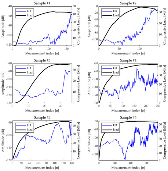
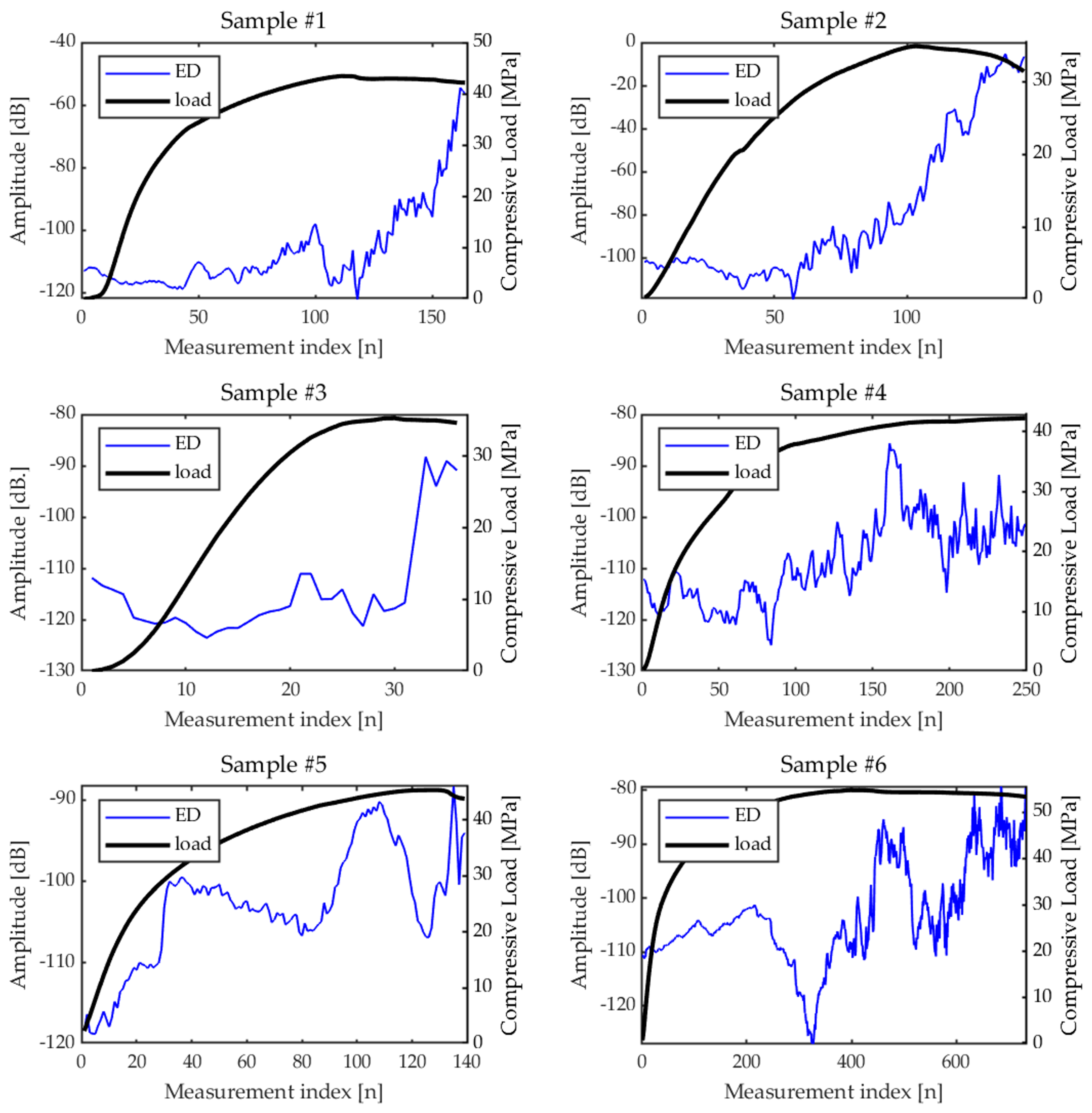
Figure 24. ED trend for all the samples tested.

This is a particularly interesting set of features, whose combination with time-of-flight ones can provide a way to detect changes in the specimen and, in particular, the onset of cracks.

$Max{E}_1$ also tends to exhibit an initial plateau, followed by a decline, and then another plateau. We hypothesize that the decline coincides with the onset of microcracking. $Max{E}_2$ behaves similarly, though we must consider that: (1) the noise level affects $Max{E}_2$ significantly more than $Max{E}_1$, and (2) the opening of cracks can increase the energy of the 2nd harmonic, so there are two effects that act in opposition. The traveling energy decreases as the cracks open, but cracks enhance the 2nd harmonic energy. This could explain the sudden peaks of $Max{E}_2$ in coincidence with the local fallings of $Max{E}_1$, and the fact that in general $Max{E}_2$ decay is slower with respect to $Max{E}_1$.

The behavior of $MaxE$’s features reflects on the Energy Distortion parameters, $ED$s. Figure 24 shows the evolution of $ED$ across the six samples.

Similar to the ToF features, $ED$ increases as the compression increases, and sometimes the rise has some steps in coincidence with changes of $ToF$’s features that should correspond to the onset of nonlinear behavior in the specimen under pressure. $ED$ is also affected by the measurement noise: notably, for all the samples, $ED$ starts around the value $-110$ dB, which is actually determined by the noise level, including possible nonlinearities of the measurement system, as the 2nd harmonic contribution due to cracks can be considered negligible at the beginning of the compression. On the other hand, by continuing to increase the compression, the energy of both $h_1\left(t\right)$ and $h_2\left(t\right)$ would ideally tend to very small values (see $MaxE$’s plots) determined by their noise standard deviation. In the middle, between the lower and the upper limit, $ED$ increases, as well as the weight of the 2nd harmonic. It could therefore be reasonable to set a threshold value for which, once $ED$ crosses and surpasses the threshold, the sample can be considered damaged with open cracks. A $10 \mathrm{d}\mathrm{B}$ increase from the initial value seems to be a possible value for the threshold.

In summary, considering the results among all samples, we believe that $ToF{E}_1$ is the most robust parameter, showing consistent behavior over the several tested specimens, and better performance than all the other time-of-flight features, including $To{F}^{AIC}$, for both early detection and in severe cracking conditions. In addition, $ToF{E}_2$, although for some samples is quite noisy, is largely more robust among all features extracted from $h_2\left(t\right)$, and also it starts to increase significantly earlier than $ToF{E}_1$. Furthermore, this does not imply that the other extracted features are useless; rather, they may provide valuable insights in more specific cases, depending on the particular characteristics of the specimen under investigation. In particular, a damage index defined from a combination of the energy-based features from the 1st and 2nd harmonics could be a good indicator of the state of health of the sample. This will be investigated in future works.

4. Discussion

This study defined an ultrasonic procedure capable of estimating the linear and nonlinear response of the sample under test to be used for the NDE and SHM of concrete. The method has been applied to various samples, and a set of features has been extracted and compared to identify those capable of producing robust and repeatable results in the (early) detection of the cracking. The analysis focused in particular on various features related to the time-of-flight, extracted from both the linear and nonlinear response thanks to the properties of the ESS-PuC procedure. While time-of-flight is routinely used in concrete NDE, to our knowledge $ToF$ is estimated for the first time from the nonlinear response of the sample. This can lead to a significant improvement in the early detection of cracks, as these are expected to induce harmonic generation. Further, we also showed that the $ToF$ features extracted from the cumulative energy are more robust than the others for both linear and nonlinear part. Some other features extracted from the energy signals were also introduced that can be used together with those related to the $ToF$ to define a damage index. This will be the subject of future work encompassing also the use of features extracted from the frequency analysis of the linear and nonlinear responses and the direct characterization of the $\sigma -ϵ$ with strain instrumentation as a reference for the validation of the damage index.

References

- Shah, A.; Ribakov, Y. Non-linear ultrasonic evaluation of damaged concrete based on higher order harmonic generation. Mater. Des. 2009, 30, 4095–4102. [Google Scholar] [CrossRef] [Scilit]
- McCann, D.; Forde, M. Review of NDT methods in the assessment of concrete and masonry structures. NDT Int. 2001, 34, 71–84. [Google Scholar] [CrossRef] [Scilit]
- Breysse, D. Nondestructive evaluation of concrete strength: An historical review and a new perspective by combining NDT methods. Constr. Build. Mater. 2012, 33, 139–163. [Google Scholar] [CrossRef] [Scilit]
- Rehman, S.K.U.; Ibrahim, Z.; Memon, S.A.; Jameel, M. Nondestructive test methods for concrete bridges: A review. Constr. Build. Mater. 2016, 107, 58–86. [Google Scholar] [CrossRef] [Scilit]
- Taheri, S. A review on five key sensors for monitoring of concrete structures. Constr. Build. Mater. 2019, 204, 492–509. [Google Scholar] [CrossRef] [Scilit]
- Zhu, Z.; Mediamartha, B.M.; Yu, S.; Li, Y.; Xu, J.; Gu, P. Simulation of the Mesoscale Cracking Processes in Concrete Under Tensile Stress by Discrete Element Method. Materials 2025, 18, 2981. [Google Scholar] [CrossRef] [Scilit]
- Peng, R.x.; Qiu, W.l.; Jiang, M. Application of a micro-model for concrete to the simulation of crack propagation. Theor. Appl. Fract. Mech. 2021, 116, 103081. [Google Scholar] [CrossRef] [Scilit]
- Karaiskos, G.; Deraemaeker, A.; Aggelis, D.; Van Hemelrijck, D. Monitoring of concrete structures using the ultrasonic pulse velocity method. Smart Mater. Struct. 2015, 24, 113001. [Google Scholar] [CrossRef] [Scilit]
- Gondim, R.M.L.; Haach, V.G. Monitoring of ultrasonic velocity in concrete specimens during compressive loading-unloading cycles. Constr. Build. Mater. 2021, 302, 124218. [Google Scholar] [CrossRef] [Scilit]
- Ivanchev, I. Investigation with non-destructive and destructive methods for assessment of concrete compressive strength. Appl. Sci. 2022, 12, 12172. [Google Scholar] [CrossRef] [Scilit]
- Zhang, W.; Yang, J.; Ren, L.; Dou, H.; Chen, X.; Jia, H.; Mao, Y.; Zhang, J.; Xu, W.; Zhou, H.; et al. High-Performance Capacitive Ultrasonic Transducer for Non-Destructive Testing of Concrete Compressive Strength. Sensors 2025, 25, 4903. [Google Scholar] [CrossRef] [Scilit] [PubMed]
- Laureti, S.; Ricci, M.; Mohamed, M.; Senni, L.; Davis, L.A.; Hutchins, D.A. Detection of rebars in concrete using advanced ultrasonic pulse compression techniques. Ultrasonics 2018, 85, 31–38. [Google Scholar] [CrossRef] [Scilit]
- Antonaci, P.; Bruno, C.L.E.; Gliozzi, A.; Scalerandi, M. Monitoring evolution of compressive damage in concrete with linear and nonlinear ultrasonic methods. Cem. Concr. Res. 2010, 40, 1106–1113. [Google Scholar] [CrossRef] [Scilit]
- Park, S.J.; Kim, G.J.; Kwak, H.G. Characterization of stress-dependent ultrasonic nonlinearity variation in concrete under cyclic loading using nonlinear resonant ultrasonic method. Constr. Build. Mater. 2017, 145, 272–282. [Google Scholar] [CrossRef] [Scilit]
- Castellano, A.; Fraddosio, A.; Piccioni, M.D.; Kundu, T. Linear and nonlinear ultrasonic techniques for monitoring stress-induced damages in concrete. J. Nondestruct. Eval. Diagn. Progn. Eng. Syst. 2021, 4, 041001. [Google Scholar] [CrossRef] [Scilit]
- Basu, S.; Thirumalaiselvi, A.; Sasmal, S.; Kundu, T. Nonlinear ultrasonics-based technique for monitoring damage progression in reinforced concrete structures. Ultrasonics 2021, 115, 106472. [Google Scholar] [CrossRef] [Scilit]
- Seo, W.; Lee, S.; Baek, S.; Shin, D.M.; Youm, K.; Kim, B.; Kim, G.; Yun, T.S. Utilizing linear and nonlinear ultrasound for improved estimation of concrete strength. Nondestruct. Test. Eval. 2025, 1–17. [Google Scholar] [CrossRef] [Scilit]
- Kim, G.; Loreto, G.; Kim, J.Y.; Kurtis, K.E.; Wall, J.J.; Jacobs, L.J. In situ nonlinear ultrasonic technique for monitoring microcracking in concrete subjected to creep and cyclic loading. Ultrasonics 2018, 88, 64–71. [Google Scholar] [CrossRef] [Scilit]
- Kim, G.J.; Park, S.J.; Kwak, H.G. Experimental characterization of ultrasonic nonlinearity in concrete under cyclic change of prestressing force using Nonlinear Resonant Ultrasonic Spectroscopy. Constr. Build. Mater. 2017, 157, 700–707. [Google Scholar] [CrossRef] [Scilit]
- Weiss, F.J.; Kim, J.Y.; Kurtis, K.E.; VanderLaan, D.; Tenorio, C.N.; Jacobs, L.J. Experimental study on the nonlinear mixing of ultrasonic waves in concrete using an array technique. NDT Int. 2024, 143, 103054. [Google Scholar] [CrossRef] [Scilit]
- Farina, A. Simultaneous measurement of impulse response and distortion with a swept-sine technique. In Proceedings of the 108th Convention of the Audio Engineering Society, Paris, France, 19–22 February 2000; pp. 1–24. [Google Scholar]
- Müller, S.; Massarani, P. Transfer-function measurement with sweeps. J. Audio Eng. Soc. 2001, 49, 443–471. [Google Scholar]
- Dietrich, P.; Masiero, B.; Vorländer, M. On the optimization of the multiple exponential sweep method. J. Audio Eng. Soc. 2013, 61, 113–124. [Google Scholar]
- Novak, A.; Simon, L.; Lotton, P.; Gilbert, J. Chebyshev model and synchronized swept sine method in nonlinear audio effect modeling. In Proceedings of the 13th International Conference on Digital Audio Effects (DAFx-10), Graz, Austria, 6–10 September 2010; p. 15. [Google Scholar]
- Schmitz, T.; Embrechts, J.J. Hammerstein kernels identification by means of a sine sweep technique applied to nonlinear audio devices emulation. J. Audio Eng. Soc. 2017, 65, 696–710. [Google Scholar] [CrossRef] [Scilit]
- Rébillat, M.; Hennequin, R.; Corteel, E.; Katz, B.F. Identification of cascade of Hammerstein models for the description of nonlinearities in vibrating devices. J. Sound Vib. 2011, 330, 1018–1038. [Google Scholar] [CrossRef] [Scilit]
- Ege, K.; Boutillon, X.; Rébillat, M. Vibroacoustics of the piano soundboard:(Non) linearity and modal properties in the low-and mid-frequency ranges. J. Sound Vib. 2013, 332, 1288–1305. [Google Scholar] [CrossRef] [Scilit]
- Rébillat, M.; Hajrya, R.; Mechbal, N. Nonlinear structural damage detection based on cascade of Hammerstein models. Mech. Syst. Signal Process. 2014, 48, 247–259. [Google Scholar] [CrossRef] [Scilit]
- Novak, A.; Simon, L.; Kadlec, F.; Lotton, P. Nonlinear system identification using exponential swept-sine signal. IEEE Trans. Instrum. Meas. 2009, 59, 2220–2229. [Google Scholar] [CrossRef] [Scilit]
- Burrascano, P.; Di Schino, A.; Versaci, M. Efficient estimation of synthetic indicators for the assessment of nonlinear systems quality. Appl. Sci. 2024, 14, 9259. [Google Scholar] [CrossRef] [Scilit]
- Burrascano, P.; Di Bella, A.; Gliozzi, A.; Laureti, S.; Ricci, M.; Rizwan, M.K.; Scalerandi, M.; Tortello, M. A comparison of scaling subtraction and pulse compression methods for the analysis of elastic nonlinearity. In Proceedings of the Meetings on Acoustics; Acoustical Society of America: Melville, NY, USA, 2019; Volume 38, p. 065013. [Google Scholar]
- Novak, A.; Simon, L.; Lotton, P. Synchronized swept-sine: Theory, application, and implementation. J. Audio Eng. Soc. 2015, 63, 786–798. [Google Scholar] [CrossRef] [Scilit]
- Laureti, S.; Burrascano, P.; Zito, R.; Ricci, M. Optimal tapering data window for exponential swept-sine identification of non-linear systems models. Measurement 2023, 219, 113283. [Google Scholar] [CrossRef] [Scilit]
- Burrascano, P.; Laureti, S.; Senni, L.; Ricci, M. Pulse compression in nondestructive testing applications: Reduction of near sidelobes exploiting reactance transformation. IEEE Trans. Circuits Syst. I Regul. Pap. 2018, 66, 1886–1896. [Google Scholar] [CrossRef] [Scilit]
- Kurz, J.H.; Grosse, C.U.; Reinhardt, H.W. Strategies for reliable automatic onset time picking of acoustic emissions and of ultrasound signals in concrete. Ultrasonics 2005, 43, 538–546. [Google Scholar] [CrossRef] [Scilit] [PubMed]
Disclaimer/Publisher’s Note: The statements, opinions and data contained in all publications are solely those of the individual author(s) and contributor(s) and not of MDPI and/or the editor(s). MDPI and/or the editor(s) disclaim responsibility for any injury to people or property resulting from any ideas, methods, instructions or products referred to in the content. |
© 2026 by the authors. Licensee MDPI, Basel, Switzerland. This article is an open access article distributed under the terms and conditions of the Creative Commons Attribution (CC BY) license.