


Abstract
Response spectra (RS) provide an efficient link between earthquake ground motions and structural demand. Still, rare event screening for long-period, resonance-sensitive systems is often approximated by applying uniform multipliers to a design-basis earthquake (DBE) spectrum to represent beyond-design-basis earthquake (BDBE) levels. This paper develops critical excitation (CE) based response spectra (CE-RS) as a spectrum-format, low-overhead screening tool that makes period-local resonance sensitivity explicit while remaining anchored to code-defined hazard levels. This paper develops CE-RS as a response-spectrum-based screening tool for identifying period-local resonance sensitivity at code-defined hazard levels by using the CE framework to search, within an admissible set defined by bounded power spectral density (PSD) content and intensity constraints, for the input that maximizes structural response. Code-based target spectra are adopted as hazard anchors, consistent with the intent of probabilistic seismic hazard analysis (PSHA), at representative sites in Australia (Canberra; AS 1170.4:2024, Site Class Be) and the United States (San Francisco; ASCE/SEI 7-22, Site Class BC). For each site, a spectrum-compatible seed accelerogram is generated to reproduce the 5% damped target spectrum and to calibrate admissible-set bounds using peak ground acceleration (PGA), peak ground velocity (PGV), and Arias intensity. CE is then performed period-by-period over the long-period range to obtain CE-RS ordinates, which are compared with the DBE target and conventional BDBE-type references formed by uniform spectrum scaling. The resulting framework provides a code-comparable, site-anchored interpretation of long-period demand influenced by resonance effects, supporting rapid prioritization in preliminary design and in the screening of existing long-period-sensitive infrastructure for strengthening/rehabilitation.
1. Introduction
Low-probability but high-consequence earthquakes are of particular concern because they can impose demands well beyond routine design-level shaking, especially in long-period-sensitive structures and infrastructure systems. Even when collapse is prevented, damage to lifelines and supporting networks (e.g., power, transportation, water, and communications) can reduce the functionality of critical facilities and can slow post-event response and recovery. Because these impacts can spread across interconnected systems, resilience-oriented planning often requires credible, transparent, and efficient screening methods. This allows sites, systems, and retrofit options to be ranked and prioritized without running full-time history analyses in the first stage [1,2,3]. In this setting, spectrum-based representations remain attractive. Response spectra (RS) provide a compact summary of peak dynamic response across structural periods and damping levels, which makes it practical to compare ground-motion demand with key structural properties and performance limits. Combined with simple acceptance checks (e.g., drift limits, acceleration-sensitive components, or isolator displacement), spectra support fast decisions in both design and assessment. They can help identify cases where more detailed nonlinear analysis is warranted [4,5,6].
The RS is based on the peak response of a family of linear single-degree-of-freedom (SDOF) oscillators, all of which experience the same ground-acceleration time history. Each oscillator is defined by its natural period, while the same specified damping ratio (e.g., 5%) is used for all oscillators, and its maximum response (e.g., spectral acceleration) is recorded. In this way, a single acceleration record is transformed into a period-dependent demand measure that is easier to use in engineering decision-making [1,4]. This transformation provides designers with a practical link between earthquake loading and structural dynamics, enabling demand to be compared with the governing structural period and damping without running repeated response-history analyses for every early-stage check. It also highlights how strongly seismic demand depends on spectral shape, damping assumptions, and the period range that controls a given structure or component. More recent hazard- and reliability-consistent spectral concepts clarify this link by relating the target spectral ordinates directly to Probabilistic Seismic Hazard Analysis (PSHA) outputs (e.g., hazard curves, uniform-hazard spectra, or related conditional spectra) and to stated performance or risk objectives, which improves alignment between code intent and expected performance [3,5,6,7,8].
Despite major progress in seismic design and assessment, recent earthquakes continue to reveal demand mechanisms that are not always well represented by simplified code expectations. These include long-duration shaking that can accumulate damage over many cycles, pulse-like near-fault motions that concentrate large energy in one or a few cycles, and period bands in which recorded RS approach or exceed the design spectrum used in practice. These characteristics can increase demands on flexible systems, low-damped structures, and isolation-dominated configurations, and they can also affect the functionality of critical facilities even when life-safety goals are met [1,8,9,10].
The 2011 Tohoku earthquake sequence further underscored these concerns, producing strong, long-duration shaking and widely reported long-period effects that affected high-rise and other long-period-sensitive structures. These lessons supported a broader beyond-design-basis-earthquake (BDBE) mindset, especially for systems where very low-probability events can still govern risk and public consequences [11,12].
In nuclear safety practice in particular, post-event guidance and more recent international standards emphasize explicit consideration of BDBE and margin-type evaluations. In this setting, seismic safety is often demonstrated using complementary approaches, such as seismic margin assessment (SMA), seismic probabilistic safety assessment (SPSA), and risk-informed combinations, with attention to avoiding cliff-edge behavior and ensuring that safety-significant structures, systems, and components (SSCs) maintain required functions under rare excitations [13,14,15,16].
The evolution of seismic provisions in the United States has moved toward risk-consistent ground motions and a tighter connection to current PSHA products, rather than relying solely on fixed prescriptive force levels [6,17,18,19,20,21,22,23,24,25]. Recent national earthquake hazards reduction program (NEHRP) [17,18] and American Society of Civil Engineers/Structural Engineering Institute Standard 7-22 (ASCE/SEI 7-22) [19] developments also put more weight on period-dependent demand, because the same site can be controlled by different hazard mechanisms at short, moderate, and long periods. As a result, multi-period response spectra (MPRS) were introduced to avoid defining the spectrum solely by two anchor periods, which can understate demand in some soft-soil and longer-period cases [17,18,19,20]. At the same time, the risk-targeted maximum considered earthquake (MCER) framework continues to receive attention because deterministic components and constraints (including the deterministic spectrum and the deterministic lower-limit spectrum) can govern the final spectral ordinates in some locations and period ranges [21,22,23]. Finally, studies of updated United States hazard models show that changes in ground-motion models and basin/site effects can shift mapped spectral values across periods, thereby affecting collapse-risk estimates and, in turn, shaping retrofit or mitigation priorities [13,24,25].
A parallel shift is underway in Australia. National-scale PSHA updates, along with efforts to verify hazard maps against observed shaking, have supported a more transparent and evidence-based approach to seismic design actions. This is particularly important in a stable continental region setting, where earthquake rates and ground-motion models remain uncertain [26,27,28]. The National Seismic Hazard Assessment of Australia (NSHA) integrated updated source models and ground-motion models within a logic-tree framework that explicitly accounts for model uncertainty. This uncertainty propagates to code-calibrated hazard levels and to the RS used for structural design and assessment. Subsequent work has compared how different generations of Australian hazard maps with the mapped distribution of estimated strong shaking from an atlas of historical ShakeMaps. This provides an additional, large-scale check on map performance at commonly used design-level exceedance probabilities (e.g., 10% in 50 years) [28]. This ongoing integration of new research into practice is also reflected in the updated national loading standard, which revises the framework for translating hazards into design response spectra (DRS) and actions [29].
At the same time, resilience goals increasingly extend beyond life safety to post-earthquake functionality, especially for facilities and networks that support response and recovery. Empirical and modeling-based studies of vital buildings and nonstructural/equipment systems show that serious service disruption can occur even without global structural collapse, because utilities, equipment, and other nonstructural components are often controlled by floor accelerations and period-dependent demand in specific ranges [27,28,29,30,31,32,33]. This makes screening tools valuable for quickly identifying possible demand amplification and resonance sensitivity before committing to large nonlinear analysis suites. However, rare event evaluation is commonly carried out using large sets of recorded or simulated motions, spectrum matching, and hazard-consistent selection/scaling (e.g., conditional-spectrum-based targets). While these methods are valuable for detailed assessment, they can be resource-intensive when the objective is rapid identification of the response features governing seismic demand and a clear, code-compatible description of how that demand varies with structural period [34,35,36,37,38].
Critical excitation (CE) methods provide a complementary approach to evaluating seismic demand. Instead of selecting specific recorded motions, CE searches for the most unfavorable input within an admissible set defined by clear bounds (e.g., limits on input energy, peak intensity, or power spectral density (PSD) constraints), while maximizing a chosen structural response measure [39,40,41,42,43,44]. The resulting motion can be interpreted as a conservative, system-dependent upper-envelope excitation tailored to the structure under study, helping reveal which parts of the frequency content are most critical. This viewpoint is particularly useful when near-resonance or narrow-band amplification controls response, because CE-type formulations (and related impulse-based critical inputs) intentionally focus on the period ranges that maximize displacements, drifts, or accelerations. Recent studies have also extended these ideas to long-period systems, including base-isolated structures, indicating that rare event screening can benefit from explicit attention to spectral shape and resonance potential, rather than relying solely on a single scalar intensity measure [45,46,47].
The present study is motivated by the idea that CE can be formulated as a practical spectral tool for engineering design. The goal is to retain the clear, period-based interpretability of response spectrum methods while adding a rational, resonance-focused bound suitable for rare events, such as BDBE. Accordingly, we developed a CE-based response spectrum (CE-RS) as a simple, fast screening tool for assessing infrastructure demand under rare earthquakes. The method is intended to minimize the need for uniform scaling factors by maintaining a clear link between code intent and expected performance to (i) hazard concepts used in modern practice, (ii) code-style spectral formats, and (iii) key dynamic properties that control resonance-sensitive response. The proposed workflow supports practical use by enabling rapid comparison of predicted critical spectral demands against acceptance criteria and by providing a transparent basis for progressing from screening to targeted nonlinear assessment only when screening indicates potential concern. Compared with conventional BDBE-style practice that assumes a uniform scaling of the DBE spectrum, the proposed CE-RS does not assume that reserve beyond the code spectrum is represented by a single amplitude multiplier applied equally across all periods. Instead, it provides a period-specific bound by redistributing admissible input intensity in time and frequency under fixed constraints. Compared with suite-based record selection, spectrum matching, or detailed nonlinear time history analysis, the CE-RS is not intended to replace site-specific verification but to provide a lower-overhead screening layer in response spectrum format that remains directly comparable to code spectra. Relative to earlier resonance-focused CE or impulse-based critical-input studies, the novelty here is the translation of CE into a code-anchored response spectrum overlay for rapid screening of long-period-sensitive systems under rare event conditions. In this paper, the main contributions are (i) a CE-to-spectrum translation that yields conservative, resonance-sensitive demand bounds for rare earthquake screening; (ii) a computationally efficient implementation workflow compared with full suite-based nonlinear analyses; and (iii) an evaluation strategy consistent with current code and hazard-model directions in the United States and Australia, while keeping the method applicable beyond nuclear-only contexts.
2. Code-Based Target Spectra
The RS provide a practical bridge between ground-motion hazard and structural demand by mapping the characteristics of a ground acceleration record into peak responses of idealized SDOF oscillators over a range of periods. Because seismic sources, attenuation characteristics, and site conditions vary by region, the resulting hazard-consistent spectral ordinates are inherently location dependent. Accordingly, national design standards codify region-specific target RS (and associated parameters) to provide a transparent, implementable basis for engineering design and assessment that is consistent with each region’s adopted hazard model and performance intent.
2.1. Australia Code
In the Australian building standard (AS 1170.4:2024) [29], the horizontal earthquake action for spectrum-based procedures is expressed through a codified response spectrum, in which the period-dependent demand is described by a small set of hazard and site parameters rather than by a record-derived spectrum. Australian standard AS 1170.4 is developed for buildings and is used here only as a reference spectrum format and a hazard-anchoring framework for design-oriented comparison of period-dependent demand. Specifically, the standard defines an elastic site hazard spectrum (dimensionless, for horizontal loading) and a corresponding horizontal design response spectrum used in equivalent-static and dynamic analysis, where denotes the vibration period of the mode/SDOF oscillator, in seconds [29].
The spectrum level is first anchored to a target hazard through the annual probability of exceedance and the associated probability factor , where is selected based on the adopted limit state and hazard level (Table 1). The geographic hazard level is captured by the hazard design factor , which is defined by the standard for each location using either tabulated values or mapped contours. The values of the parameters used in this study are reported in Table 1.
Table 1.
Summary of hazard anchoring parameters for AS 1170.4:2024 spectra used in this study [29].
To maintain a minimum national hazard floor (particularly relevant to stable continental regions), the standard imposes a lower bound on , and this lower-bound check is also documented in Table 1 to ensure consistent spectrum anchoring across sites and return periods. Contemporary Australian PSHA developments (e.g., NSHA18) have shown that long-return-period hazard estimates can shift as source characterization and ground motion modeling are updated, which directly affects how -anchored spectrum should be interpreted across periods [26].
Given and , AS 1170.4:2024 constructs the elastic site hazard spectrum through the dimensionless spectral shape factor , which depends on the site sub-soil class (Ae–Ee) and period [29]. The standard’s definitions align the key spectra as:
and the design spectrum as:
where is the dimensionless structural performance factor, and indicates the dimensionless structural ductility factor, reflecting the intended inelastic energy dissipation and system robustness in design. In dynamic analysis, the standard explicitly permits using as the ground motion representation (modal response spectrum analysis) and also recognizes site-specific DRS and time history suites, provided their RS approximate the target site spectrum. In the Australian engineering literature, codified spectral-shape models of this type are often discussed in terms of their influence on flexible systems and their sensitivity to the definition of the long-period branch, particularly in low-to-moderate seismicity settings. More detailed code-interpretation and detailing discussions [48,49,50] further emphasize that the practical meaning of and must be consistent with the achieved detailing and deformation capacity.
The core of the Australian spectrum shape is , which AS 1170.4:2024 as both listed ordinates and an equivalent closed-form (piecewise) definition, enabling straightforward numerical implementation [29]. The spectral shape factor is given by ref. [29]:
where is the dimensionless short-period intercept, indicates the short-period slope (units of 1/s), controls the branch (units of s), denotes the dimensionless plateau cap, and controls the long-period decay (units of ). The soil-class-specific coefficient sets adopted in this paper are shown in Table 2. These coefficients are obtained directly from AS 1170.4:2024 and reproduce the code expressions precisely for each site class. This formulation introduces two fixed corner periods, (end of the short-period) and (the beginning of the long-period decay). In addition, a soil-dependent transition period defines where the upper-bound operation switches from the constant plateau to the hyperbolic branch . Softer site classes yield larger . The standard also specifies upper and lower values (notably at ) for use in modal RS and numerical-integration time history procedures, as well as in parts-and-components force calculations; these corresponding values should be applied consistently when reproducing spectra for those applications.
Table 2.
Coefficient sets for the normalized spectral shape factor.
Figure 1 provides a schematic illustration of the normalized Australian DRS shape (normalized spectral acceleration versus period) prescribed in AS 1170.4:2024, included to emphasize the general form of the spectrum and its key transitions (short-period rise, mid-period plateau behavior, and long-period decay) in a way that is visually consistent with the plotting style used throughout this manuscript. The curves are intentionally illustrative and not tied to any particular site, hazard level, or soil profile. They are intended to reproduce the standard’s spectral shape intent for the normalized factor , without relying on any particular geographic input. For completeness and for direct implementation, the corresponding (non-normalized) spectra are obtained by scaling Figure 1 using Equations (1) and (2). The appropriate and values are selected from Table 1, and the minimum requirement is then enforced so that the anchoring level used in the spectrum construction satisfies the code floor condition.
Figure 1.
Illustrative comparison of code-based response spectrum forms: (a) ASCE response spectrum forms and (b) Australian response spectrum form.
A key limitation of this codified approach is that, while it is transparent and practical, a fixed shape may not capture all period-by-period features of a fully site-specific hazard spectrum, such as a uniform hazard spectrum (UHS). This limitation is more pronounced where epistemic uncertainty is substantial and long-return-period ordinates are sensitive to modeling assumptions and data limitations [26,48]. AS 1170.4:2024 acknowledges this limitation by permitting site-specific DRS and by requiring spectrum-compatibility checks when time history suites are used, indicating that the piecewise provided in the standard should be viewed as a standardized reference shape, rather than a definitive period-by-period hazard description for every site. This motivates complementary rare event (beyond-design) screening concepts that retain the usability of RS while more directly interrogating period-specific demand concentration mechanisms that can govern critical infrastructure response [48,49,50].
2.2. ASCE-7 Code
In ASCE/SEI 7-22, design ground motions for spectrum-based seismic procedures are represented by codified RS, rather than by the RS computed from individual accelerograms. The code framework is anchored to risk-targeted MCER hazard values. It provides practical spectra for routine applications, such as the equivalent lateral force (ELF) procedure and RS-based dynamic analysis. In current ASCE 7-22 practice, two spectrum representations are commonly used: (i) a conventional two-anchor (two-period) DRS and (ii) an MPRS derived from hazard-consistent ordinates at multiple discrete periods, typically obtained through the ASCE Hazard Tool and the underlying United States Geological Survey (USGS) seismic design database/services [17,18,19,20,21,51].
Within the ASCE 7 framework, the 5%-damped spectral acceleration at vibration period is expressed as . The risk-targeted MCER hazard is characterized by the mapped spectral ordinates and , corresponding to the short-period range and the 1.0 s period, respectively, defined for reference site conditions and retrieved from the hazard database/tools for the specified location and risk category [19]. These mapped values originate from PSHA, which combines contributions from seismic sources, recurrence behavior, and ground motion prediction models to produce period-dependent, hazard-consistent spectral accelerations. This probabilistic foundation underpins current national hazard models and the development of risk-targeted design parameters [3,17,18,19,20,21]. Accordingly, both the conventional two-period spectrum and the MPRS should be viewed as PSHA-based code representations of the selected hazard level, with the key distinction being how spectral shape is constructed across periods.
After applying site effects, the corresponding MCER parameters are and , and the design spectral values are defined by the standard scaling:
where sets the short-period constant-acceleration level, while governs the intermediate-to-long-period amplitude of the design spectrum [6]. Within this framework, the ASCE 7 design-based earthquake (DBE) is commonly interpreted as the design-level event represented by the code DRS (i.e., approximately two-thirds of the MCER hazard level across periods). In practical terms, this means that the DRS used for ELF and linear dynamic analysis corresponds to a DBE-consistent target spectrum. At the same time, MCER provides the upper-level hazard anchor that defines the DBE spectrum through the prescribed scaling.
In the two-period DRS, the spectrum shape is described by a small set of characteristic periods. Two primary corner periods are defined as follows:
Also, a long-period transition period is obtained from the hazard database and controls the onset of the long-period decay [19]. Using these parameters, the conventional two-period spectrum can be expressed in a compact piecewise form as follows:
which is commonly interpreted as a rising short-period segment transitioning to constant-acceleration, then constant-velocity, and finally a constant-displacement tail. This representation provides a direct mapping from the two anchor ordinates (, ) and to a continuous design spectrum suitable for standard linear procedures.
ASCE/SEI 7-22 additionally recognizes that a spectrum reconstructed solely from (, ) can smooth out period-dependent hazard features that are important for some sites and structural periods. The primary motivation for shifting beyond a two-period approximation is that a fixed three-segment functional shape may not preserve the frequency content implied by PSHA at intermediate and moderately long periods, particularly for soft-soil sites and for regions where large-magnitude contributions govern long-period ordinates. This behavior was documented during the technical development of the 2020 NEHRP Provisions [17,18] and was carried forward in ASCE/SEI 7-22 [19] through the introduction of MPRS concepts intended to better represent hazard-consistent spectral shape across periods.
To address this limitation, the MPRS is defined using a set of hazard-consistent spectral ordinates evaluated explicitly at multiple periods, rather than derived from a prescribed three-segment shape. In implementation, the USGS seismic design services provide the multi-period MCER spectrum at a fixed period grid for a specified site location and site class, and the corresponding design MPRS is obtained by applying the two-thirds factor at each period:
where the linear interpolation was used to evaluate between discrete points for continuous plotting and analysis use [17,18,19,20,21,51]. Also, denotes the discrete period set provided by the hazard tool output, and is the total number of defined periods. Accordingly, the MPRS can be interpreted as a DBE-consistent spectrum defined period-by-period, but without imposing the fixed two-anchor spectral shape assumption introduced by Equation (8). Figure 1 schematically compares the ASCE/SEI 7 two-parameter DRS and the MPRS, included for illustration only to highlight their conceptual differences. The two-parameter form enforces a prescribed piecewise shape between a small set of control points. In contrast, the MPRS is defined directly by discrete hazard-consistent ordinates over period (with interpolation used only to draw a continuous curve).
In ASCE 7-22 workflows, the MPRS is typically accessed directly through the hazard-tool outputs, rather than manually assembling a generic spectral shape. In addition, the MPRS preserves the location- and site-class-dependent frequency content implied by the hazard model over a broad range of periods. In practical usage, the process includes (i) specifying the site latitude–longitude and the adopted site class, (ii) obtaining the multi-period MCER ordinates from the hazard database, and (iii) computing the design MPRS by applying the two-thirds factor to each ordinate, with intermediate periods obtained by interpolation. For plotting purposes, the MPRS is obtained by connecting the discrete design ordinates using linear interpolation over the period axis, yielding a continuous curve suitable for comparison against the conventional spectrum. For practical extension of the spectrum beyond the largest listed period, implementations commonly maintain compatibility with long-period decay logic by adopting the same long-period transition period to control the long-period tail behavior.
From a design-procedure standpoint, ASCE/SEI 7-22 includes both the two-period spectrum and the MPRS, and the selection depends on the analysis method and the availability of multi-period data. In this sense, the two-period representation serves as a compact, easily parameterized spectrum for conventional design checks. In contrast, the MPRS provides a target spectrum that more directly reflects the mapped multi-period hazard ordinates for spectrum-based dynamic analysis and for applications where intermediate-to-long-period shape details response.
3. CE Method
A convenient way to view earthquake loading in the random vibration setting is through its PSD. The PSD provides a compact frequency domain description of how input spectral content is distributed across angular frequencies, and it is therefore directly tied to resonance-driven response. This viewpoint is particularly valuable for rare event screening, because extreme demands in flexible systems can arise not only from large amplitudes but also from an unfavorable concentration of input energy near response-sensitive frequency bands, even when conventional intensity metrics are not unusually high. Modern CE formulations leverage this fact by treating the PSD as a decision variable and posing an optimization problem, and among all admissible PSDs satisfying explicit bounds, identifying the one that maximizes a specified response measure [39,40,41,42,43,44,45,46,47].
The central idea of CE originated from early robust excitation concepts and was subsequently developed through probabilistic representations and optimization-based solution procedures. Contemporary CE research (including long-period and isolation-focused developments) continues this line of development by combining analytically interpretable input models with intensity-consistent admissible sets to produce conservative, mechanism-based demand bounds compatible with RS engineering practice [45,46,47]. In this framework, the excitation is described as a finite-duration nonstationary process, so that both the time-localization and the frequency allocation of the input can be controlled in a physically meaningful way [52].
A commonly used nonstationary representation introduces a deterministic modulation of a stationary Gaussian component, written as:
where is a zero-mean stationary Gaussian process characterized by the two-sided PSD . Also, indicates a deterministic envelope function that modulates the amplitude in time. The envelope represents the transient nature of earthquake shaking and therefore bounds the effective time window over which the stationary frequency content can accumulate into a drift- or displacement-sensitive response. Accordingly, controls where energy is distributed in the frequency domain, while controls when that energy is delivered in time; both are required to reproduce long-duration effects and resonance-type demand amplification mechanisms in a nonstationary excitation model. As depicted in Figure 2, the envelope increases rapidly at the beginning of motion and then decays gradually, representing the transient nature of earthquake shaking (illustrated for and in Figure 2). Here, and are deterministic envelope-shape parameters that control the rise and decay characteristics of the modulation function, and the values and are shown only to illustrate a representative envelope shape in Figure 2. This time-localization imposed by ensures that the stationary component contributes to primarily within a finite effective duration.
Figure 2.
Deterministic envelope function governing the build-up and decay of the modulated excitation (shown for the illustrative envelope-shape parameters and ).
To connect the input description to structural demand, consider the linear SDOF oscillator subjected to horizontal ground acceleration :
where denotes relative displacement, and , , and are the mass, damping coefficient, and stiffness coefficient, respectively. In probabilistic CE, a response measure is selected as the optimization objective. For long-period-sensitive problems, displacement/drift measures are natural candidates because they connect directly to performance limits in flexible and isolation-dominated systems [45,46,47,52]. In the present SDOF formulation, the objective is expressed at a fixed time instant as given by:
where is a transfer function that quantifies how the spectral content around contributes to the chosen response measure at . For the adopted drift-based objective, this transfer function can be written using cosine- and sine-type response coefficients:
with
where is the impulse response of the SDOF system. These expressions make the envelope explicit. enters the response mapping directly and shapes how efficiently a narrow frequency band can build a response over the duration of interest.
A classical analytical CE result emerges when the admissible PSD family is constrained by both the total PSD area bound and a peak PSD cap as given by:
Under these constraints, the maximizing PSD at fixed becomes rectangular over an active band , and the admissible bandwidth satisfies:
The interpretation is straightforward, and the optimizer allocates the admissible spectral power to the frequency region that produces the largest increase in the objective integral (12). Since is nonnegative, the critical PSD attains the cap level over the band where the transfer function contributes most strongly. The band location is, therefore, not chosen by the analyst. It is selected by the CE optimization through the structure-dependent transfer function [33,34,35,36]. Figure 3 schematically illustrates this CE outcome.
Figure 3.
Critical excitation optimal rectangular PSD band.
With Equations (12)–(15), the CE problem can be understood as a two-level maximization: for each time instant , one first selects the optimal band to maximize under constraints (16)–(18), and then the peak response over the time window is obtained by taking the maximum over . This is consistent with the standard CE procedure in which frequency allocation is optimized for a fixed time, and the governing response is then identified over the strong motion duration implied by .
PSD bounds alone regulate frequency domain power, but they do not automatically prevent physically unrealistic solutions (e.g., excessively concentrated content inconsistent with credible intensity measures). CE implementations, therefore, often supplement Equations (16)–(18) with constraints that explicitly link the admissible set to engineering-relevant intensity or cumulative measures. A widely used cumulative constraint is the Arias intensity, expressed as [52]:
together with the admissibility requirement:
This bound regulates the overall acceleration-squared content and thus limits cumulative intensity in a manner consistent with the strong motion severity measures used in practice. To prevent unrealistically narrow spectral concentration, a complementary limit is often introduced in the frequency domain through the Fourier amplitude spectrum:
where is the Fourier amplitude spectrum of . Under these combined bounds, an approximate link can be established between the implied admissible bandwidth, the cumulative intensity cap, and the amplitude limit:
which provides a practical rationale for combining cumulative and amplitude-type limitations when constructing physically admissible long-period critical inputs.
For long-period applications, an additional velocity-type constraint is often used to prevent very low frequencies from dominating and to keep the resulting excitation realistic for displacement-sensitive response. As illustrated in Figure 4, this constraint preserves the CE band-selection character, energy is still concentrated within an active band of width . Still, it imposes an upper bound, indicated by , which limits the admissible peak level. As a result, the optimizing spectrum cannot degenerate into an excessively narrow, spike-like concentration. Instead, a finite-width critical band is maintained while remaining aligned with the dominant portion of the response-related spectrum .
Figure 4.
Rectangular-band excitation with upper bound and bandwidth .
Although the rectangular PSD is analytically convenient and central to many CE derivations, its sharp and narrow band edges can be overly idealized for long-period ground motion characteristics. To improve realism while retaining analytical simplicity, CE studies have proposed admissible PSD families with controlled transitions, which reduce unexpected changes while keeping the optimization logic driven by . Such a family adopts a piecewise low–mid–high arrangement [53]:
where the transition width is , and and denote corner frequencies. In this definition, is selected so that the total PSD area meets the prescribed admissibility constraints, while the overall shape avoids a perfectly flat band (see Figure 5).
Figure 5.
CE-optimal two-level PSD allocation under total-power and peak-cap constraints and the modified –– shape.
4. Site Selection
Seismic design codes prescribe region-dependent elastic RS because both hazard level and expected shaking frequency content vary by location. Consequently, the target spectrum is not universal, and it changes with the selected geographic location and the assumed site condition in each standard. In this study, two benchmark regions were selected to support a controlled comparison between (i) a stable-continent (intraplate) environment where hazard is generally moderate but can be locally elevated, and (ii) a plate-boundary environment characterized by frequent strong ground shaking. The selected sites are Canberra (Australia) and San Francisco (USA), and the corresponding site conditions are taken as site class Be (AS 1170.4) and the mapped/reference site class BC (ASCE 7-22). This selection ensures that the comparison is performed across two leading design frameworks while preserving a clear contrast in tectonic setting and hazard level.
4.1. Canberra
In AS 1170.4:2024, the regional seismic hazard for design is expressed through the hazard design factor . The standard specifies that may be obtained either from its provided list based on each region or, when a site is not listed, from the hazard contours mapped for the relevant exceedance level and reference site class [26].
Canberra is a convenient Australian reference site because it is explicitly listed in the standard, enabling a transparent and reproducible spectrum definition in this study; the adopted value and the corresponding used for the selected hazard level are summarized in Table 1. The Australian site condition is defined using the site sub-soil class system (Ae–Ee). In this work, site class Be is adopted to represent a reference rock condition consistent with both the standard’s definitions and the national hazard products [26,27,28,29]. AS 1170.4:2024 defines class (Be) as a rock site characterized by a low-amplitude natural site period less than 0.15 s, or rock meeting strength/velocity criteria, including an average shear wave velocity over the top 30 m exceeding 760 m/s.
The regional justification for selecting Canberra is further supported by the Australian hazard map [27], which is included solely to illustrate regional hazard variation across Australia and is not used to derive the design spectra adopted in this study. NSHA18 provides uniform-probability hazard maps for 10% and 2% in 50 years for PGA and multiple periods. These products explicitly demonstrate the regional variation in seismic hazard across Australia and provide PGA mapping consistent with the Australian code site class definition. As shown in Figure 6, Canberra lies in a relatively higher-hazard area compared with many other regions, making it a useful national benchmark for comparison.
Figure 6.
Australia-wide PGA hazard map for 10% probability of exceedance in 50 years (AS 1170.4; site class Be).
In addition, Canberra provides a representative case for Australian intraplate seismicity, where damaging earthquakes may occur within the interior of a tectonic plate rather than at an active plate boundary. This makes it suitable for representing a stable-continent hazard scenario within a modern design framework. Figure 7 presents the Canberra DRS constructed using the formulation and the hazard-anchoring parameters described above. This spectrum serves as the code-consistent target spectrum for the Australian site in this study.
Figure 7.
Site-specific seismic design spectrum for Canberra.
4.2. San Francisco
For the United States, ASCE/SEI 7-22 defines the design spectrum as a function of site location and site class, with spectra obtained through the USGS seismic design mapping infrastructure [21,54,55]. ASCE 7-22 notes that the MPRS are available through the ASCE hazard-tool workflow [54] and are tied to the USGS design database services [55]. In practical terms, this is implemented through the USGS ASCE 7-22 design web service, which accepts the site coordinates, risk category, and site class as inputs, and returns both two-period and multi-period spectra, including the MCER and design forms.
San Francisco is selected as the United States benchmark because it represents a high-hazard, plate-boundary-dominated environment [19]. The San Francisco Bay Area is controlled by the broad San Andreas transform plate-boundary system, where the Pacific Plate moves laterally past North America, producing frequent shallow earthquakes across multiple major faults. This tectonic setting makes San Francisco an appropriate upper-hazard reference case for spectrum comparison against an Australian intraplate site.
A second practical reason for selecting this region is that the San Francisco Bay Area is influenced by well-documented active faults (including the Hayward Fault system), which contribute to its high ground motion hazard and are widely recognized in regional hazard assessments [56,57,58]. The San Francisco RS adopted in this study (Figure 8) is, therefore, used to emphasize that the selected U.S. site represents a high seismic-hazard environment suitable for the purpose of this study.
Figure 8.
Site-specific multi-period seismic design spectrum for San Francisco.
For the site condition, site class BC is adopted because the mapped parameters and are defined for that reference condition, and the ASCE/SEI 7-22 design-maps web service provides outputs for BC. In the mapping framework, BC denotes the B/C boundary reference condition [58], which keeps the United States spectra consistent with the reference site definition underlying the national hazard outputs.
5. Numerical Procedure, Results, and Discussion
Region-dependent RS were defined for Canberra (AS 1170.4:2024, site class Be) (Figure 7) and San Francisco (ASCE/SEI 7-22, site class BC) (Figure 8), and these spectra were used as hazard-consistent anchors for all later steps [19,29]. For San Francisco, the ASCE multi-period spectrum was adopted because it preserves the period-by-period spectral shape available in the ASCE framework and is more suitable for evaluating resonance-sensitive long-period demand, whereas for Canberra, the Australian target spectrum was taken directly in its native codified AS 1170.4 form, since that standard does not use the same multi-period spectrum distinction. Since both standards express design demand through site- and class-dependent spectra, the goal is not to judge one code against another. Instead, the aim is to examine how each code-based target spectrum translates into a CE-based long-period bound when the excitation must remain compatible with the same hazard level at each site.
For each site, the 5%-damped code target spectrum was plotted together with conventional BDBE-type references obtained by uniformly scaling the DBE ordinates, consistent with common practice in the literature for defining BDBE [59,60]. As shown in Figure 9 and Figure 10, three scaling levels were used (150%, 167%, and 200% of DBE) to provide a simple and transparent baseline for comparison with subsequent CE-RS. Figure 9 shows the Canberra RS with its scaled references, and Figure 10 illustrates the same construction for San Francisco. These uniformly scaled curves are included only as code-compatible BDBE-type reference levels. These scaling levels were not selected arbitrarily. They were adopted as representative BDBE-style uniform-scaling reference levels consistent with common code- and literature-based practice, including refs. [59,60], and are used here only as transparent comparison baselines rather than as unique hazard-equivalent definitions.
Figure 9.
Canberra BDBE response spectra, scaled to 150%, 167%, and 200% of DBE.
Figure 10.
San Francisco BDBE response spectra, scaled to 150%, 167%, and 200% of DBE.
Next, for both Canberra and San Francisco, a spectrum-compatible seed accelerograms were generated using SeismoArtif [61]. The seed motions were used only to match the site-specific 5%-damped code target spectrum within a selected tolerance and to provide site-consistent baseline values of PGA, PGV, and Arias intensity for subsequent constraint calibration. This follows common spectrum-matching practice, where an input record is adjusted, in the time or frequency domain, to reproduce a target spectral shape while maintaining reasonable duration and nonstationary character [62,63]. Using the site-specific code spectrum to calibrate the seed motions ties the overall shaking level to each site’s hazard-consistent target and avoids an arbitrary amplitude assumption. In SeismoArtif, the site-specific 5%-damped target response spectrum was given as the input target, and the artificial seed record was generated so that its response spectrum matched that target spectrum within the selected tolerance. The resulting spectrum-compatible seed motion was then used as a reference record for extracting the baseline intensity measures required in the CE procedure.
After seed generation, intensity- and energy-related metrics were extracted to calibrate to the allowable set used in the CE construction. PGA and PGV were taken as complementary amplitude limits, and Arias intensity was used as a cumulative intensity bound. More specifically, the Arias intensity constraint and its admissibility are given by Equations (19) and (20), while the complementary amplitude/frequency-domain limitation is represented through Equations (21) and (22). The PGA and PGV bounds were calibrated from the spectrum-compatible seed motions and then imposed in the CE procedure as site-specific input limits. This step is critical to interpreting the results. The CE procedure is not allowed to increase demand simply by increasing the overall input level. Once PGA/PGV/Arias bounds are fixed, any increase in response should come mainly from how the motion allocates its content in time and frequency (i.e., resonance-focused concentration) under those credible limits, which is consistent with the CE philosophy for a bounded worst-case search.
With the site-calibrated bounds defined, the CE construction was carried out period-by-period over the long-period range considered in this study. For each target period , an admissible excitation was optimized under the prescribed constraints. The resulting CE motion was then evaluated through the 5%-damped elastic response spectrum to obtain the ordinate . Repeating this step across all periods yields a discrete CE-RS. The influence of the seed motion on the final CE-RS is, therefore, indirect rather than prescriptive. Different spectrum-compatible seeds may lead to some change in the final ordinates through the calibrated PGA, PGV, Arias intensity, and mismatch tolerance, but once these bounds are fixed, the period-by-period CE optimization governs the resulting CE-RS shape and level, rather than the detailed waveform of the seed motion itself. This pointwise construction reflects the basic intent of critical excitation, and it maximizes a chosen response quantity by concentrating input content near the period of interest, while still meeting physically meaningful bounds.
The resulting overlays are shown in Figure 11 for Canberra and Figure 12 for San Francisco. In each figure, the CE-RS is plotted together with the code spectrum and the uniformly scaled BDBE-type RS. The discussion is intentionally focused on the long-period range (, because many long-period-sensitive systems (e.g., base-isolated structures, long-span bridges, and liquid storage tanks) are often governed by displacement and resonance effects rather than by short-period acceleration demand alone. For these systems, critical behavior may appear as localized peaks over a narrow period band, rather than a uniform upward shift of the entire spectrum. This pattern is consistent with CE formulations that maximize resonance-sensitive response under PGA, PGV, and Arias Intensity constraints [39,40,41,42,43,44,45,46,47].
Figure 11.
Canberra response spectra comparison, including DBE, BDBE, and the CE spectrum.
Figure 12.
San Francisco response spectra comparison, including DBE, BDBE, and the CE spectrum.
A key motivation for introducing the CE-RS is that conventional spectrum checks, even with uniform scaling, do not always make resonance sensitivity over specific periods explicit in the long-period tail. Several CE-based studies on isolated systems and liquid storage tanks report that resonance-driven peaks can control demand even when overall intensity measures are not extreme, because the governing mechanism is an unfavorable alignment between dominant input content and the system’s long-period dynamics [4,5,6,7,8,9,10,11,12,13,14,15,16,17,18,19,20,21,22,23,24,25,26,27,28,29,30,31,32,33,34,35,36,37,38,39,40,41,42,43,44,45,46,47,53]. In this paper, the CE-RS overlay is, therefore, used as a resonance-aware supplement to the code spectrum. It keeps the hazard anchor (i.e., the site code spectrum) fixed, while testing whether credible time–frequency concentration can produce a higher long-period ordinate than the code target and its uniformly scaled references.
From the viewpoint of Figure 11 and Figure 12, the overlay compares two different definitions of margin in the long-period range: (i) an amplitude-only margin represented by uniform scaling of the DBE spectrum (BDBE-style) and (ii) a period-dependent bound given by the CE-RS, obtained by redistributing admissible intensity in time and frequency under the same site-anchored PGA/PGV/Arias constraints. Over the long-period branch , this distinction is especially clear, since uniform scaling preserves the original spectral shape and increases all ordinates by the same factor, whereas the CE-RS selectively amplifies the periods for which resonance-focused redistribution is most effective under the same fixed constraints. As a result, the CE-RS can exceed the uniformly scaled references over specific long-period bands, thereby making localized resonance-sensitive demand more explicit than a single global scaling factor. The overlay plots can be interpreted as a period-by-period envelope check under fixed intensity bounds. Where the CE-RS lies below the code spectrum (or below a chosen uniformly scaled DBE reference), the corresponding baseline curve envelopes the resonance-focused bound in that period range under the adopted PGA/PGV/Arias constraints, indicating that the selected DBE/BDBE reference is conservative for resonance effects in that band. Where the CE-RS lies between DBE and a uniformly scaled DBE reference, the code-level spectrum alone may not envelope the resonance-focused bound. Still, the selected scaling level does so, implying that the adopted BDBE-style margin also covers the period-local amplification indicated by the CE-RS. Where the CE-RS exceeds a uniformly scaled reference over a narrow period band, the result indicates that a single global multiplier may not fully envelope a period-local resonance bound under the same intensity limits. This should be treated as a screening flag motivating closer checks in that band, rather than as evidence of a higher hazard level or a deficiency in the code spectrum.
A more detailed interpretation of Figure 11 and Figure 12 is that the difference between the CE-RS and the uniformly scaled DBE references is period-local rather than uniform over the whole spectrum. In other words, the CE-RS does not indicate a general increase in demand at all periods but highlights long-period bands in which resonance-focused amplification becomes more pronounced than that implied by a single global scaling factor. This is evident in the contrast between Canberra and San Francisco. For Canberra, the CE-RS exceeds the DBE/BDBE references mainly for periods greater than about 3 s, whereas for San Francisco, it remains above these conventional references over essentially the full plotted period range. This difference indicates that the CE-RS does not act as a simple uniform upward scaling of the code spectrum but responds to the site-specific target spectral shape and the corresponding admissible constraints. In the present comparisons, the PGA, PGV, and Arias intensity limits were not adjusted during the optimization, but were fixed from the spectrum-compatible seed motions generated for each site, so the observed differences reflect redistribution of admissible input content in time and frequency, rather than an arbitrary increase in the overall shaking level.
This resonance-sensitive, period-local behavior becomes more relevant when the performance objective is tied to continued operation and serviceability. In that case, displacement-sensitive demands (e.g., isolator stroke, long-period drift limits, tank convective/impulsive measures, or equipment-sensitive response measures) can control decisions even when short-period metrics appear moderate. Recent CE applications with bounded PSD constraints highlight the benefit of capturing resonance sensitivity clearly while remaining consistent with the site hazard level. This includes studies that introduce secondary long-period bounds for displacement-sensitive systems and studies aimed at BDBE-style screening [45,46,47]. Related observations also appear in the base-isolation literature, where long corner-period conditions and low-frequency input can increase displacement demand and shift the focus from strength checks to displacement-controlled targets [64]. Applied studies further show that response control and tuning can depend strongly on the effective period and damping of isolated systems, which supports the need for period-focused checks when selecting or adjusting isolation solutions [65].
From a performance-based viewpoint, the CE-RS can be interpreted as a resonance-aware demand bound that complements the probability-based intent of PSHA-derived code spectra. Code spectra provide hazard-consistent ordinates by period, but they are not intended to explicitly enforce worst-case resonance concentration at a particular long period. In contrast, CE does not assign an exceedance probability to the constructed motion. Instead, it provides an upper-bound estimate of a response ordinate under clearly stated constraints that are anchored to the same site level. In this sense, the CE-RS can be used to assess whether a long-period design may be susceptible to plausible resonance amplification beyond what is implied by the code spectrum shape or by conventional uniform scaling. This interpretation is consistent with displacement-based discussions for base-isolated systems, where performance is often governed by displacement-related limits and in-structure demands rather than by force-based indicators alone [65,66,67].
In practical safety-margin terms, the distinction is that uniform scaling implies a single global reserve beyond the DBE spectrum, whereas the CE-RS examines whether that apparent reserve remains adequate when admissible input content is concentrated near a structurally sensitive long period. This is especially important for long-period-sensitive systems, where the controlling demand is often displacement-driven and localized around the effective period rather than represented by a uniform increase over all periods. Accordingly, if the CE-RS approaches or exceeds the code spectrum or a selected uniformly scaled reference over a narrow period band, the result should be interpreted as a reduction of usable safety margin in that band, not as evidence of a different hazard level. For critical infrastructure, this provides a practical risk-screening benefit. It helps identify cases in which resonance-sensitive demand may threaten isolator displacement capacity, long-period drift limits, liquid storage tank response, or other displacement-controlled performance measures, thereby indicating where more detailed verification, operational review, or retrofit prioritization may be warranted under the same site-anchored intensity bounds.
The overlays can also support an early-stage decision workflow. During preliminary design, the engineer often needs to understand whether the selected dynamic characteristics, such as effective period and damping, place the system in a range where long-period demand is highly resonance-sensitive. The CE-RS provides a screening check for that purpose. It tests whether a resonance-focused, bounded excitation can produce a critical long-period demand near the intended design period. If the check indicates elevated sensitivity around a specific period band, it provides a clear reason to move to a more detailed assessment (for example, a record-suite study or nonlinear verification targeted at displacement-controlled measures). If the CE-RS indication remains moderate relative to the baseline comparisons, it supports—within the adopted constraints—the conclusion that the selected long-period range is less vulnerable to narrow-band resonance amplification at the same hazard level.
The same logic extends to existing assets and rehabilitation planning. For structures known to be long-period sensitive, rehabilitation decisions often depend on whether displacement capacity margins may be challenged in rare events. The CE-RS helps frame this question in a code-comparable format by showing where resonance-focused demand may concentrate relative to the code spectrum and a conventional scaled reference. In this setting, the CE-RS is not used to declare safety on its own. The proposed CE-RS formulation is derived from a linear SDOF representation with a prescribed damping ratio. The resulting bound is therefore conditional on the assumed period and damping level, and may be less representative for systems with substantially different or response-dependent damping behavior. In addition, soil effects are incorporated here indirectly through the site-specific target spectrum and the seed-based calibration of the admissible constraints, rather than through explicit modelling of nonlinear site response or soil–structure interaction. Accordingly, cases governed by pronounced structural nonlinearity, basin effects, nonlinear site behavior, or soil–structure interaction should be treated as outside the direct scope of the present screening formulation and examined through more detailed analysis. CE-RS helps prioritize which period bands and response measures deserve closer attention, and it supports transparent communication of why a strengthening or retrofit option is being considered (for example, the CE-RS can show where long-period spectral demand concentrates relative to the code spectrum and a conventional scaled reference while satisfying the same constraints).
Two practical points are essential for correct interpretation. First, a pointwise CE-RS is assembled from different optimized motions at different periods . For each period in the adopted grid, a separate CE optimization is solved for the corresponding SDOF oscillator. The objective function is defined for that oscillator through the response transfer function in Equations (12)–(15), so the admissible excitation redistributes its time–frequency content toward the frequencies that contribute most strongly to the response at that period, while still satisfying the same PGA/PGV/Arias Intensity. Repeating this procedure period-by-period yields the CE-RS and makes localized resonance effects explicit, rather than representing them through a single global scale factor. Therefore, the CE-RS should be read as a spectrum-format bound, not as a single time history that simultaneously maximizes all periods. Second, the bound is conditional on the selected constraints (PGA/PGV/Arias intensity) and the seed-based calibration. Taken together, these points suggest that the CE-RS can serve as a simple, rapid, spectrum-format performance check for both new designs and existing systems. It directly evaluates resonance sensitivity by testing whether a bounded, resonance-focused excitation can generate localized long-period demand amplification near the effective period. Such amplification can govern displacement-sensitive response even when overall intensity measures are not extreme, and it may exceed what is implied by the code spectrum and uniform scaling alone. For transparency and reproducibility, these values should be reported together with the seed-generation mismatch tolerance and the adopted period grid. With these clarifications, the CE-RS overlays in Figure 10 and Figure 11 provide a code-comparable, site-anchored representation of resonance-focused long-period demand that remains physically constrained by explicit intensity measures.
6. Conclusions
In this study, we developed the CE-RS as a response spectrum format screening tool for rare event seismic demand, with an emphasis on long-period, resonance-sensitive systems. The method is meant as a quick, complementary check for early design, helping identify resonance-sensitive period bands. It also supports retrofit/rehabilitation screening by indicating where displacement demand may concentrate in the long-period range. A key feature is that the CE admissible set is anchored to the site hazard level defined by the code target spectrum, rather than being set by an assumed uniform scaling factor. For Canberra (AS 1170.4:2024, Site Class Be) and San Francisco (ASCE/SEI 7-22, Site Class BC), spectrum-compatible seed motions were generated from the code targets and used to calibrate PGA, PGV, and Arias intensity bounds; under these fixed limits, any increase in long-period response arises mainly from time–frequency redistribution rather than from raising overall input level.
The resulting CE-RS is period-dependent and non-uniform, in contrast to BDBE-type screening based on uniform spectrum multipliers. This matters for long-period systems where displacement-sensitive performance can be governed by narrow-band amplification rather than short-period acceleration demand.
The overlays are read as an envelope check under fixed bounds, CE-RS below (or between) DBE, and the scaled references indicate the baseline curves envelope the resonance-focused bound in that band, whereas the CE-RS exceedance of a scaled reference flags that a single global scaling may not envelope period-local resonance demand—without implying higher hazard or a code deficiency. Practically, this supports rapid prioritization (in early design or rehabilitation planning) of which period bands require more detailed verification.
Two clarifications are essential: First, the CE-RS is assembled pointwise from different optimized motions and should be interpreted as a spectrum-format bound, not a single time history. Second, results are conditional on the adopted constraints and seed calibration; PGA/PGV/Arias values, seed-mismatch tolerance, and the period grid should be reported to ensure transparency and reproducibility.
Future work should include systematic validation against recorded and physics-based simulated motions (e.g., near-fault pulse-like inputs and long-duration subduction scenarios), sensitivity studies on admissible-set calibration and envelope modeling choices, and extensions toward nonlinear response measures and multi-degree-of-freedom (MDOF) objectives (e.g., drift, isolator displacement, base shear, and floor-response demands). In particular, future extensions should examine how the CE framework can be reformulated for nonlinear response measures and practical MDOF systems, so that period-local criticality can be evaluated not only through linear spectral ordinates but also through engineering demand parameters, such as interstory drift, isolator displacement, floor acceleration, residual deformation, and base shear. These developments will strengthen the CE-RS as a conservative, code-compatible screening tool for resilience-oriented planning and performance-based strengthening under rare earthquakes. In future code development, the CE-RS could be incorporated not as a replacement for code-defined hazard spectra, but as an additional resonance-focused screening check for long-period-sensitive systems and critical infrastructure. In that role, it may help identify cases where a conventional code spectrum or a uniform BDBE scaling factor does not fully reveal period-local demand concentration, thereby supporting more targeted verification and risk-informed design decisions.
Author Contributions
Conceptualization, A.A. and N.K.; methodology, A.A. and N.K.; software, A.A.; validation, A.A.; formal analysis, A.A. and N.K.; investigation, A.A.; resources, A.A.; data curation, A.A. and N.K.; writing—original draft preparation, A.A.; writing—review and editing, A.A. and N.K.; visualization, A.A. and N.K.; supervision, N.K. All authors have read and agreed to the published version of the manuscript.
Funding
This research was supported by the Ueda Memorial Foundation for doctoral studies.
Institutional Review Board Statement
Not applicable.
Informed Consent Statement
Not applicable.
Data Availability Statement
The original contributions presented in the study are included in the article. Further inquiries can be directed to the corresponding author.
Acknowledgments
The authors would like to appreciate three reviewers for their insightful comments and discussions on the initial manuscript. Also, the first author would like to express his appreciation to the Ueda Memorial Foundation for the scholarship he received during his Ph.D. studies at Hiroshima University.
Conflicts of Interest
The authors declare no conflict of interest.
References
- Chopra, A.K. Dynamics of Structures: Theory and Applications to Earthquake Engineering, 6th ed.; Pearson: London, UK, 2022. [Google Scholar]
- Wang, R.; Zhang, H.; Zhao, Y.-G. Evaluating Site Amplification Factor of Response Spectrum Using Microtremor Horizontal-to-Vertical Spectral Ratio. J. Earthq. Tsunami 2025, 19, 2550012. [Google Scholar] [CrossRef] [Scilit]
- Baker, J.W.; Bradley, B.A.; Stafford, P.J. Seismic Hazard and Risk Analysis; Cambridge University Press: Cambridge, UK, 2021. [Google Scholar] [CrossRef] [Scilit]
- Kim, J.K.; Park, D.; Choi, J.; Kwon, H. Response Spectral Characteristics of Moderate Earthquakes in the Southern Korean Peninsula: Implications for Seismic Design of Critical Infrastructure. Appl. Sci. 2025, 15, 13128. [Google Scholar] [CrossRef] [Scilit]
- Ji, H.Y.; Kim, J.H. Generating Input Ground Motions for Seismic Risk Assessment Using Recorded Ground Motions from the Moderate Magnitude Earthquake. Appl. Sci. 2025, 15, 640. [Google Scholar] [CrossRef] [Scilit]
- Kaviris, G.; Zymvragakis, A.; Bonatis, P.; Kapetanidis, V.; Spingos, I.; Mavroulis, S.; Kotsi, E.; Lekkas, E.; Voulgaris, N. A Logic-Tree Approach for Probabilistic Seismic Hazard Assessment in the Administrative Region of Attica (Greece). Appl. Sci. 2023, 13, 7553. [Google Scholar] [CrossRef] [Scilit]
- Xu, L.; Zhou, Z. Weighted Average Conditional Mean Spectrum (WACMS): A Bridge between Common CMS and Uniform Hazard Spectrum (UHS). Soil Dyn. Earthq. Eng. 2022, 156, 107238. [Google Scholar] [CrossRef] [Scilit]
- Chang, Z.; Gao, Q.; Monti, G.; Yu, H.; Yuan, S. Selection of Pulse-like Ground Motions with Strong Velocity-Pulses Using Moving-Average Filtering. Soil Dyn. Earthq. Eng. 2023, 164, 107574. [Google Scholar] [CrossRef] [Scilit]
- Güneş, N. Effects of Near-Fault Pulse-like Ground Motions on Seismically Isolated Buildings. J. Build. Eng. 2022, 52, 104508. [Google Scholar] [CrossRef] [Scilit]
- Dai, K.; He, Z.; Li, T.; Yang, Y. Mitigating Ground Motion Duration Impact on Steel Moment-Resisting Frames Using Viscous Dampers. J. Constr. Steel Res. 2024, 213, 108430. [Google Scholar] [CrossRef] [Scilit]
- Yön, B.; Dedeoğlu, İ.Ö.; Yetkin, M.; Erkek, H.; Calayır, Y. Evaluation of the seismic response of reinforced concrete buildings in the light of lessons learned from the February 6, 2023, Kahramanmaraş, Türkiye earthquake sequences. Nat. Hazards 2025, 121, 873–909. [Google Scholar] [CrossRef] [Scilit]
- Takewaki, I.; Fujita, K.; Yoshitomi, S. Uncertainties in long-period ground motion and its impact on building structural design: Case study of the 2011 Tohoku (Japan) earthquake. Eng. Struct. 2013, 49, 119–134. [Google Scholar] [CrossRef] [Scilit]
- International Atomic Energy Agency (IAEA). Seismic Design for Nuclear Installations; IAEA Safety Standards Series No. SSG-67; STI/PUB/1949; IAEA: Vienna, Austria, 2021. [Google Scholar]
- International Atomic Energy Agency (IAEA). Evaluation of Seismic Safety for Nuclear Installations; IAEA Safety Standards Series No. SSG-89; STI/PUB/2054; IAEA: Vienna, Austria, 2024. [Google Scholar] [CrossRef] [Scilit]
- Sarebanha, A.; Marquez, J.; Hughes, P.; Mosqueda, G. Considerations for Modeling of Base Isolated Nuclear Power Plants Subjected to Beyond Design Basis Shaking. Nucl. Eng. Des. 2021, 379, 111236. [Google Scholar] [CrossRef] [Scilit]
- Kasapoglu, B.; Sezen, H.; Aldemir, T.; Denning, R. Dynamic Seismic Probabilistic Risk Assessment of Nuclear Power Plants Using Advanced Structural Methodologies. Nucl. Eng. Des. 2024, 427, 113416. [Google Scholar] [CrossRef] [Scilit]
- Building Seismic Safety Council (BSSC). NEHRP Recommended Seismic Provisions for New Buildings and Other Structures; 2020 Edition; Volume I: Part 1 Provisions and Part 2 Commentary; FEMA P-2082-1; Federal Emergency Management Agency: Washington, DC, USA, 2020. [Google Scholar]
- Building Seismic Safety Council (BSSC). NEHRP Recommended Seismic Provisions for New Buildings and Other Structures; 2020 Edition; Volume II: Part 3 Resource Papers; FEMA P-2082-2; Federal Emergency Management Agency: Washington, DC, USA, 2020. [Google Scholar]
- ASCE/SEI 7-22; Minimum Design Loads and Associated Criteria for Buildings and Other Structures. American Society of Civil Engineers (ASCE): Reston, VA, USA, 2022.
- Tong, M.; Hanson, R.D.; Kircher, C.A.; Rezaeian, S.; Luco, N. Procedures for Developing Multi-Period Response Spectra at Non-Conterminous United States Sites; FEMA P-2078; Federal Emergency Management Agency (FEMA): Washington, DC, USA, 2020; 558p. [Google Scholar]
- U.S. Geological Survey (USGS). ASCE7-22 Web Service Documentation (Design Maps Web Service). Available online: https://earthquake.usgs.gov/ws/designmaps/asce7-22.html (accessed on 1 March 2026).
- Petersen, M.D.; Shumway, A.; Powers, P.M.; Mueller, C.S.; Moschetti, M.P.; Frankel, A.D.; Rezaeian, S.; McNamara, D.; Luco, N.; Boyd, O.S.; et al. The 2018 Update of the U.S. National Seismic Hazard Model: Where, Why, and How Much Probabilistic Ground Motion Maps Changed. Earthq. Spectra 2021, 37, 959–987. [Google Scholar] [CrossRef] [Scilit]
- Petersen, M.D.; Shumway, A.M.; Powers, P.M.; Field, E.H.; Moschetti, M.P.; Jaiswal, K.S.; Milner, K.R.; Rezaeian, S.; Frankel, A.D.; Llenos, A.L.; et al. The 2023 US 50-State National Seismic Hazard Model: Overview and implications. Earthq. Spectra 2024, 40, 5–88. [Google Scholar] [CrossRef] [Scilit]
- Federal Emergency Management Agency (FEMA). Improving Performance of Buildings in Very High-Seismic Regions—Volume 1; FEMA P-2343; Federal Emergency Management Agency: Washington, DC, USA, 2024. [Google Scholar]
- Federal Emergency Management Agency (FEMA). Improving Performance of Buildings in Very High-Seismic Regions—Volume 2; FEMA P-2343; Federal Emergency Management Agency: Washington, DC, USA, 2024. [Google Scholar]
- Allen, T.I.; Griffin, J.D.; Leonard, M.; Clark, D.J.; Ghasemi, H. The 2018 National Seismic Hazard Assessment of Australia: Quantifying Hazard Changes and Model Uncertainties. Earthq. Spectra 2020, 36, 5–43. [Google Scholar] [CrossRef] [Scilit]
- Geoscience Australia. National Seismic Hazard Assessment (NSHA). Available online: https://www.ga.gov.au/scientific-topics/community-safety/projects/nsha (accessed on 1 March 2026).
- Allen, T.I.; Ghasemi, H.; Griffin, J.D. Exploring Australian Hazard Map Exceedance Using an Atlas of Historical ShakeMaps. Earthq. Spectra 2023, 39, 985–1006. [Google Scholar] [CrossRef] [Scilit]
- AS 1170.4:2024; Structural Design Actions—Part 4: Earthquake Actions in Australia. Standards Australia Limited: Sydney, Australia, 2024.
- Cheng, Q.; Xie, L.; Wang, Z.; Liu, Z.; Lu, X.; Wang, X. Multilevel assessment method for post-earthquake functionality of medical buildings considering component–department–floor interdependencies. Reliab. Eng. Syst. Saf. 2024, 251, 110379. [Google Scholar] [CrossRef] [Scilit]
- Chavez, J.-P.; Murcia-Delso, J.; López-Almansa, F. Probabilistic framework for post-earthquake functionality assessment of seismically isolated hospital buildings using Bayesian networks. Eng. Struct. 2025, 328, 119633. [Google Scholar] [CrossRef] [Scilit]
- Shang, Q.; Li, J.; Wang, T. Floor Acceleration Response Spectra of Elastic Reinforced Concrete Frames. J. Build. Eng. 2022, 45, 103558. [Google Scholar] [CrossRef] [Scilit]
- Ding, X.; Liapopoulou, M.; Elghazouli, A.Y. Seismic Response of Non-Structural Components in Multi-Storey Steel Frames. J. Constr. Steel Res. 2024, 213, 108398. [Google Scholar] [CrossRef] [Scilit]
- Hailemikael, S.; Martini, G.; Mascandola, C.; Barani, S.; Zini, A.; Peloso, A. Application of the Conditional Spectrum Approach for the Selection of Ground Motion Time Histories in Vast Areas: An Example in the Lazio Region. Bull. Earthq. Eng. 2025, 23, 5895–5921. [Google Scholar] [CrossRef] [Scilit]
- Caicedo, D.; Karimzadeh, S.; Bernardo, V.; Lourenço, P.B. Selection and Scaling Approaches of Earthquake Time-Series for Structural Engineering Applications: A State-of-the-Art Review. Arch. Comput. Methods Eng. 2024, 31, 1475–1505. [Google Scholar] [CrossRef] [Scilit]
- Li, C.; Kunnath, S.K.; Zhao, Y. A New Framework for Ground Motion Selection for Structural Seismic Assessment. Eng. Struct. 2023, 285, 116055. [Google Scholar] [CrossRef] [Scilit]
- Demir, A.; Palanci, M.; Kayhan, A.H. Enhanced Conditional Ground Motion Selection Model Considering Spectral Compatibility and Variability of Three Components for Multi-Directional Analysis. Appl. Sci. 2025, 15, 4135. [Google Scholar] [CrossRef] [Scilit]
- Zhou, B.; Hu, J.; Yuan, C.; Wen, W.; Kong, Q. Permissible Scale Factors for Various Intensity Measures in Aftershock Ground Motion Scaling. Appl. Sci. 2023, 13, 12515. [Google Scholar] [CrossRef] [Scilit]
- Takewaki, I. Bound of Earthquake Input Energy. J. Struct. Eng. 2004, 130, 1289–1297. [Google Scholar] [CrossRef] [Scilit]
- Takewaki, I. A New Method for Non-Stationary Random Critical Excitation. Earthq. Eng. Struct. Dyn. 2001, 30, 519–535. [Google Scholar] [CrossRef] [Scilit]
- Takewaki, I. Seismic Critical Excitation Method for Robust Design: A Review. J. Struct. Eng. 2002, 128, 665–672. [Google Scholar] [CrossRef] [Scilit]
- Akehashi, H.; Takewaki, I. Pseudo-Double Impulse for Simulating Critical Response of Elastic–Plastic MDOF Model under Near-Fault Earthquake Ground Motion. Soil Dyn. Earthq. Eng. 2021, 150, 106887. [Google Scholar] [CrossRef] [Scilit]
- Akehashi, H.; Takewaki, I. Closed-Form Critical Response of Undamped Bilinear Hysteretic MDOF System under Pseudo-Double Impulse for Estimating Resonant Response under One-Cycle Sine Wave. Soil Dyn. Earthq. Eng. 2022, 157, 107254. [Google Scholar] [CrossRef] [Scilit]
- Akehashi, H.; Takewaki, I. Closed-Form Critical Response of Elastic–Plastic Shear Building with Viscous Damper under Pseudo-Double Impulse for Simulating Resonant Response under Near-Fault Fling-Step Motion. Front. Built Environ. 2022, 8, 964867. [Google Scholar] [CrossRef] [Scilit]
- Ahmadi, A.; Khaji, N.; Bazrafshan, A. Seismic analysis of base-isolated liquid storage tanks incorporating a new probabilistic long-period critical excitation method. Results Eng. 2025, 26, 104977. [Google Scholar] [CrossRef] [Scilit]
- Ahmadi, A.; Khaji, N.; Bazrafshan, A. A secondary seismic-design bound for liquid storage tanks using critical excitation methods. Mech. Based Des. Struct. Mach. 2025, 1–35. [Google Scholar] [CrossRef] [Scilit]
- Ahmadi, A.; Khaji, N.; Sadegh-Azar, H. Beyond-design-basis screening by a three-bound critical excitation envelope for base-isolated nuclear power plants. Nucl. Eng. Des. 2026, 448, 114700. [Google Scholar] [CrossRef] [Scilit]
- Tsang, H.-H. Evaluation of Codified Elastic Design Spectrum Models for Regions of Low-to-Moderate Seismicity. Soil Dyn. Earthq. Eng. 2015, 70, 148–152. [Google Scholar] [CrossRef] [Scilit]
- Menegon, S.J.; Wilson, J.L.; Lam, N.T.K.; McBean, P. RC Walls in Australia: Seismic Design and Detailing to AS 1170.4 and AS 3600. Aust. J. Struct. Eng. 2018, 19, 67–84. [Google Scholar] [CrossRef] [Scilit]
- Menegon, S.J.; Tsang, H.-H.; Wilson, J.L.; Lam, N.T.K. RC Walls in Australia: Displacement-Based Seismic Design in Accordance with AS 1170.4 and AS 3600. Aust. J. Struct. Eng. 2021, 22, 205–221. [Google Scholar] [CrossRef] [Scilit]
- Kircher, C.A.; Rezaeian, S.; Luco, N. Proposed Multi-Period Response Spectra and Ground Motion Requirements of the 2020 Recommended Provisions and ASCE 7-22. In Proceedings of the Structural Engineers Association of California (SEAOC) 2019 Convention, Squaw Creek, CA, USA, 28–31 August 2019; pp. 10–19. [Google Scholar]
- Takewaki, I. Critical Excitation Methods in Earthquake Engineering, 2nd ed.; Butterworth-Heinemann: Oxford, UK, 2013. [Google Scholar]
- Bazrafshan, A.; Khaji, N.; Ahmadi, G. A New Probabilistic Long-Period Critical Excitation Procedure for Isolated Building Structures. Mech. Based Des. Struct. Mach. 2024, 52, 7063–7091. [Google Scholar] [CrossRef] [Scilit]
- American Society of Civil Engineers (ASCE). ASCE Hazard Tool (ASCE 7 Hazard Tool). Available online: https://ascehazardtool.org/ (accessed on 1 March 2026).
- U.S. Geological Survey (USGS). Earthquake Hazard Toolbox (National Seismic Hazard Model/NSHMP Web Applications). Available online: https://earthquake.usgs.gov/nshmp/ (accessed on 1 March 2026).
- U.S. National Park Service (NPS). Transform Plate Boundaries—San Andreas Transform Plate Boundary. Available online: https://www.nps.gov/ (accessed on 1 March 2026).
- U.S. Geological Survey (USGS). Back to the Future on the San Andreas Fault (San Andreas Fault Zone as a Plate-Boundary System Including Major Bay Area Faults). Available online: https://www.usgs.gov/ (accessed on 1 March 2026).
- Wills, C.J.; Petersen, M.; Bryant, W.A.; Reichle, M.; Saucedo, G.J.; Tan, S.; Taylor, G.; Treiman, J.A. A Site-Conditions Map for California Based on Geology and Shear-Wave Velocity. Bull. Seismol. Soc. Am. 2000, 90, S187–S208. [Google Scholar] [CrossRef] [Scilit]
- Lee, S.-J.; Lee, E.-H.; Lee, C.; Park, N.-C.; Choi, Y.; Oh, C. Investigation of Seismic Responses of Reactor Vessel and Internals for Beyond-Design Basis Earthquake Using Elasto-Plastic Time History Analysis. Nucl. Eng. Technol. 2021, 53, 988–1003. [Google Scholar] [CrossRef] [Scilit]
- Kumar, M.; Whittaker, A.S.; Constantinou, M.C. Response of Base-Isolated Nuclear Structures to Extreme Earthquake Shaking. Nucl. Eng. Des. 2015, 295, 860–874. [Google Scholar] [CrossRef] [Scilit]
- Seismosoft. SeismoArtif 2025—User Help: About SeismoArtif/Accelerogram Generation (Spectrum-Compatible Accelerograms); Seismosoft: Pavia, Italy, 2025. [Google Scholar]
- Gascot, G.; Montejo, L.A. Spectrum-Compatible Earthquake Records and Their Influence on the Seismic Response of Reinforced Concrete Structures. Earthq. Spectra 2016, 32, 2061–2079. [Google Scholar] [CrossRef] [Scilit]
- Cacciola, P.; Zentner, I. Generation of Response-Spectrum-Compatible Artificial Earthquake Accelerograms with Random Joint Time–Frequency Distributions. Probab. Eng. Mech. 2012, 28, 52–58. [Google Scholar] [CrossRef] [Scilit]
- Köber, D.; Weber, F.; Lozincă, E.; Popa, V. Base Isolation Compared to Capacity Design for Long Corner Periods and Pulse-Type Seismic Records. Appl. Sci. 2023, 13, 1217. [Google Scholar] [CrossRef] [Scilit]
- Kang, Y.; Zhang, Z.; Zhang, Z.; Zhang, X.; Liu, Q. Optimal Design and Seismic Performance of Base-Isolated Structures with Varying Heights Equipped with Tuned Inerter Dampers Subjected to Far-Fault and Near-Fault Ground Motions. Appl. Sci. 2025, 15, 4739. [Google Scholar] [CrossRef] [Scilit]
- Ye, M.; Xiao, X.; Hu, Y. Direct Displacement-Based Design Procedure for Base-Isolated Building Structures Equipped with Lead Rubber Bearings. Eng. Struct. 2019, 197, 109402. [Google Scholar] [CrossRef] [Scilit]
- Jung, J.-W.; Kim, M.K.; Kim, J.H. Experimental Study on the Floor Responses of a Base-Isolated Frame Structure via Shaking Table Tests. Eng. Struct. 2022, 253, 113763. [Google Scholar] [CrossRef] [Scilit]
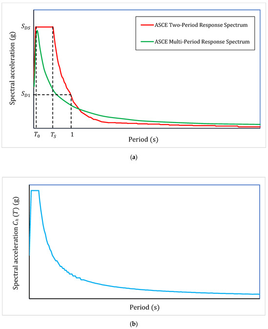
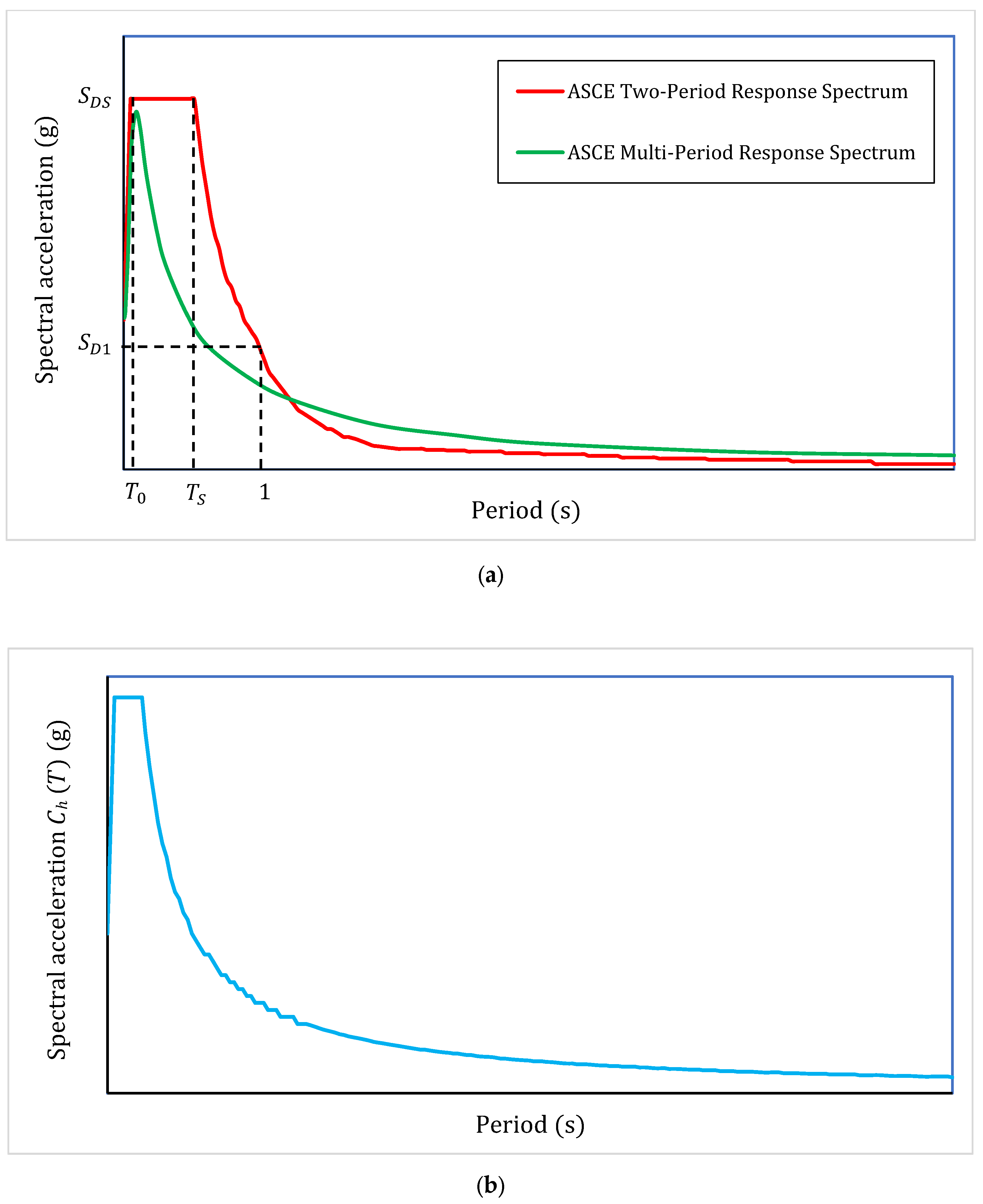
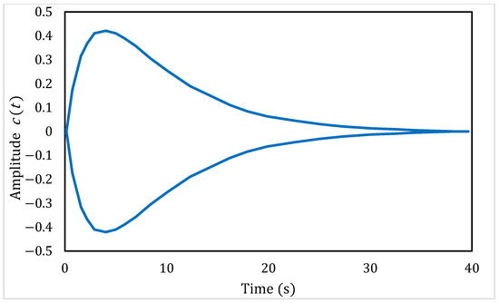
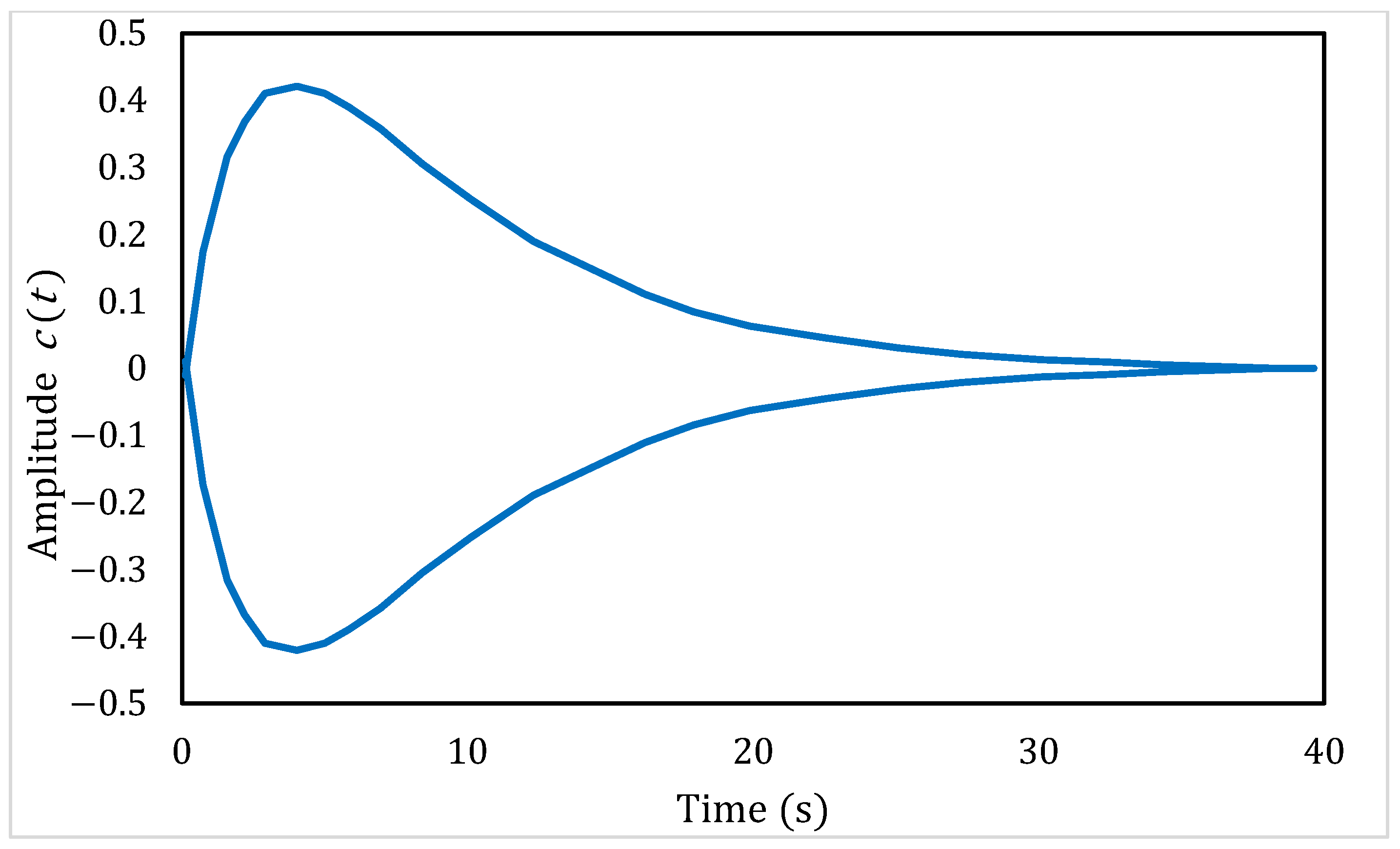
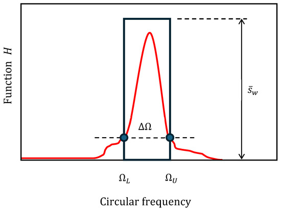
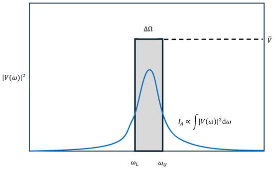
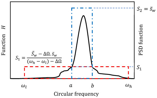
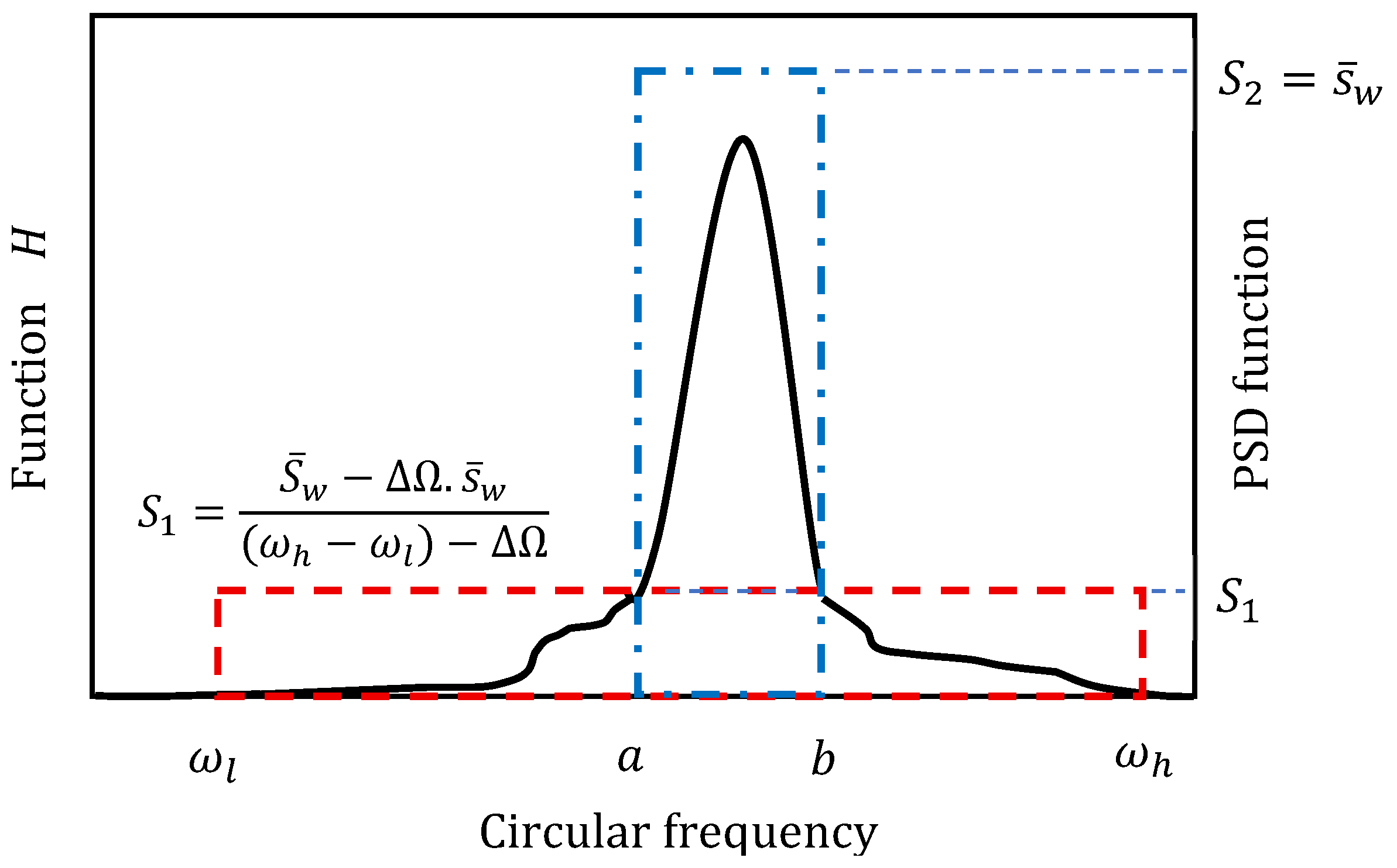
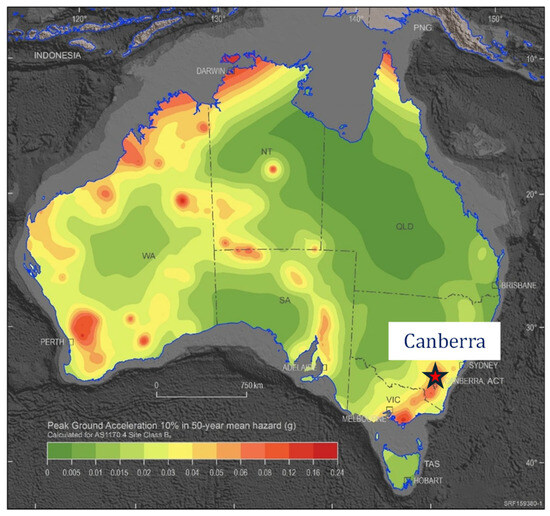
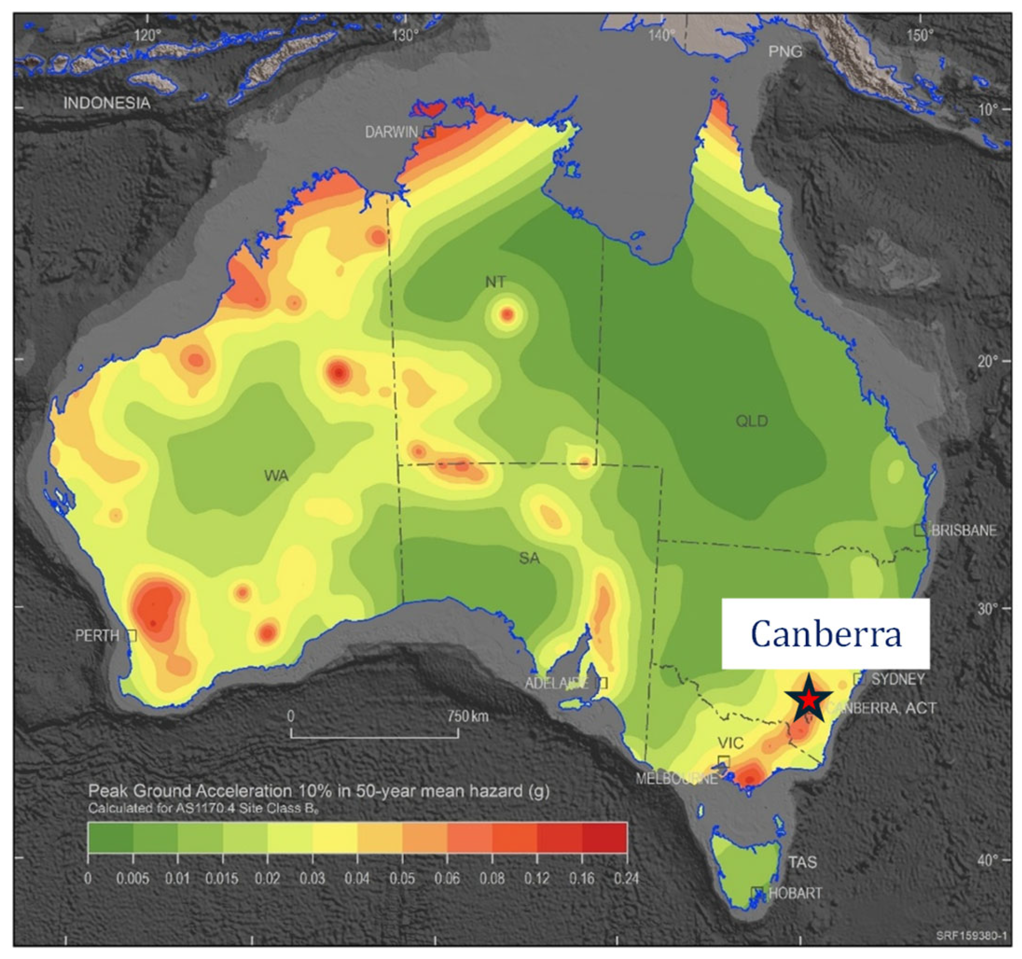
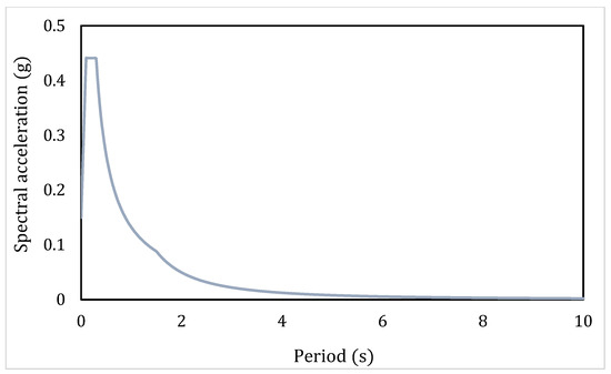
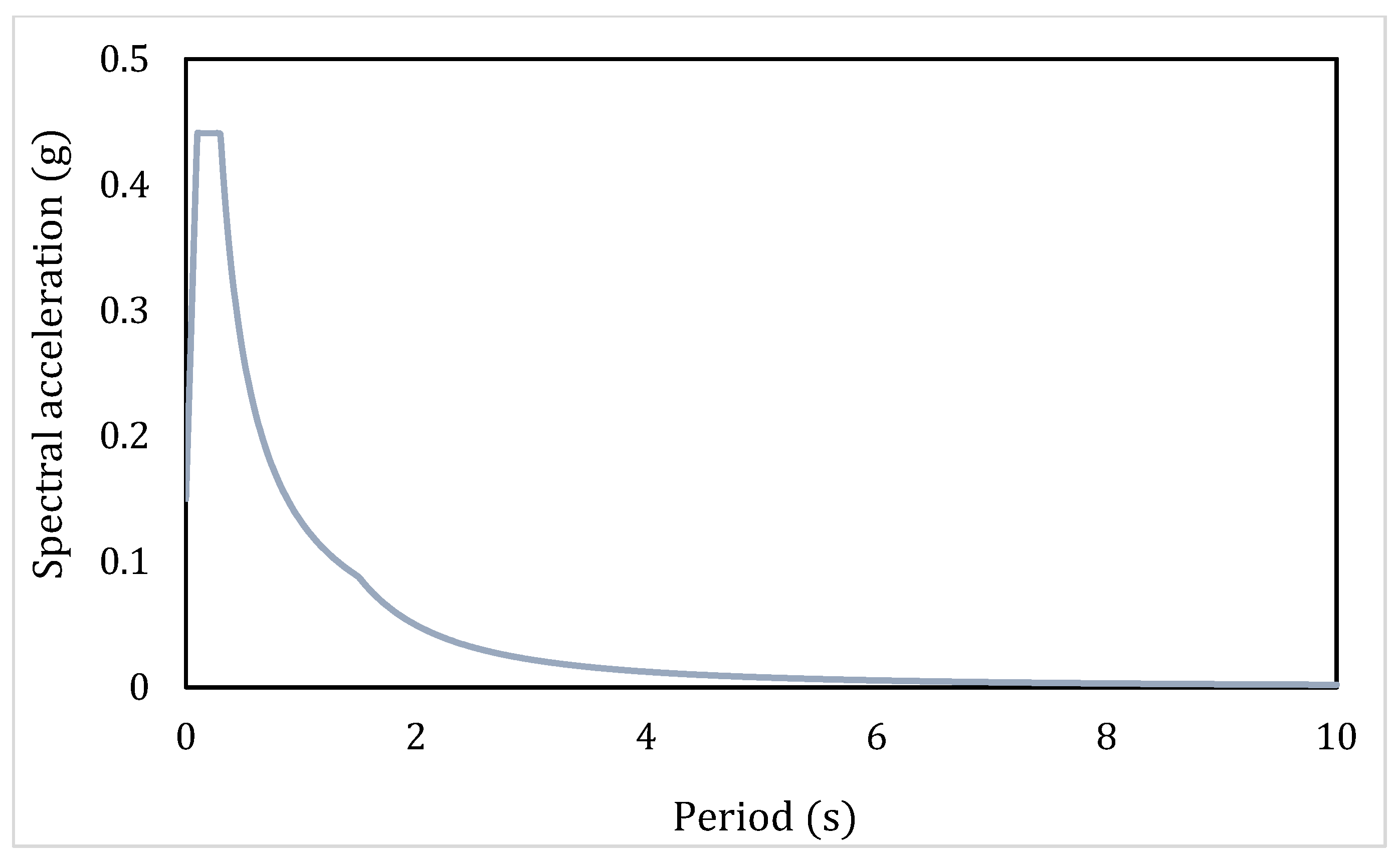
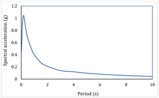
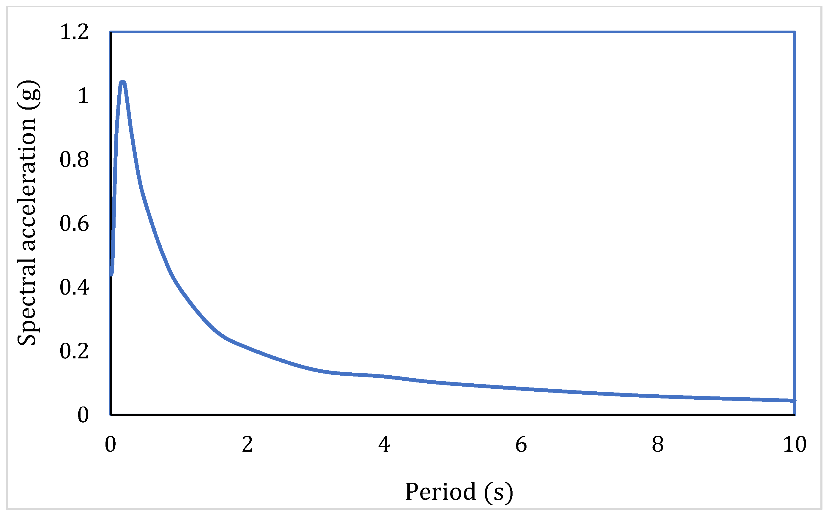
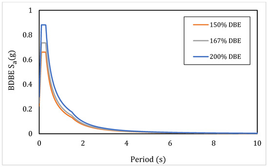
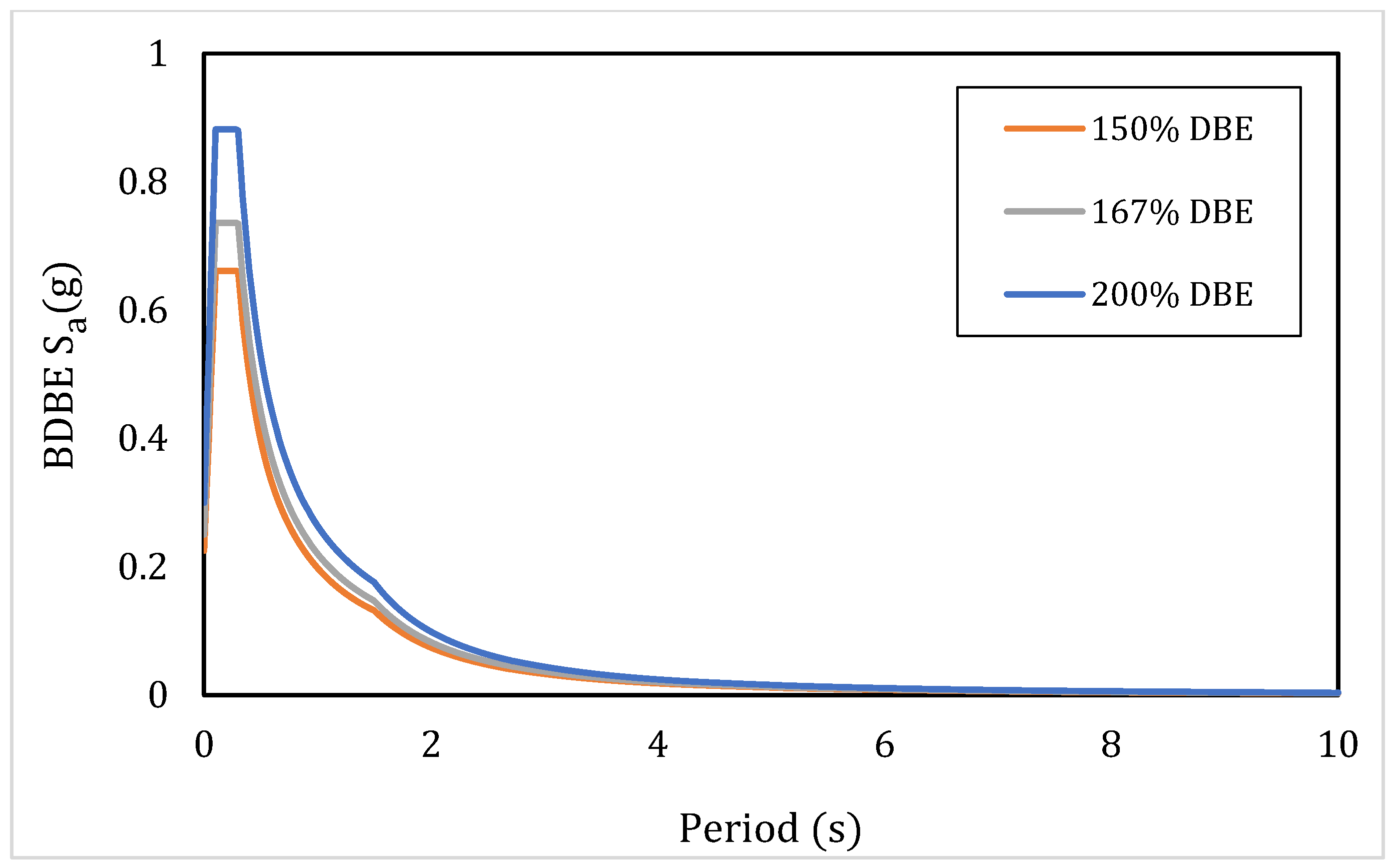
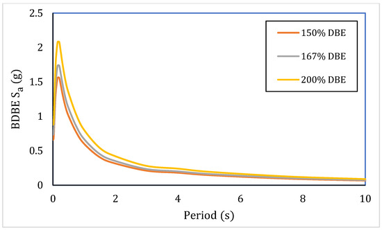
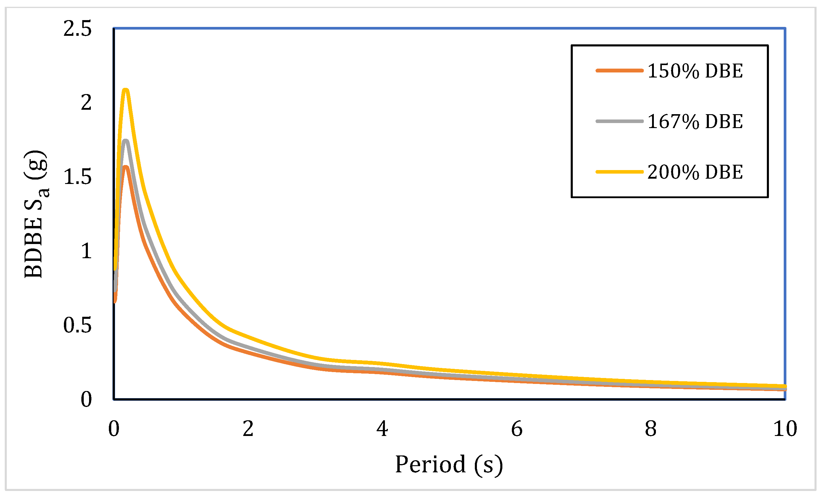
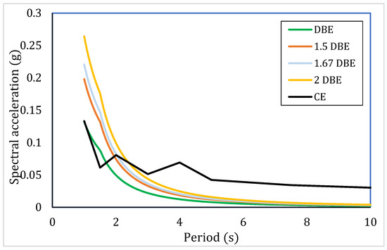
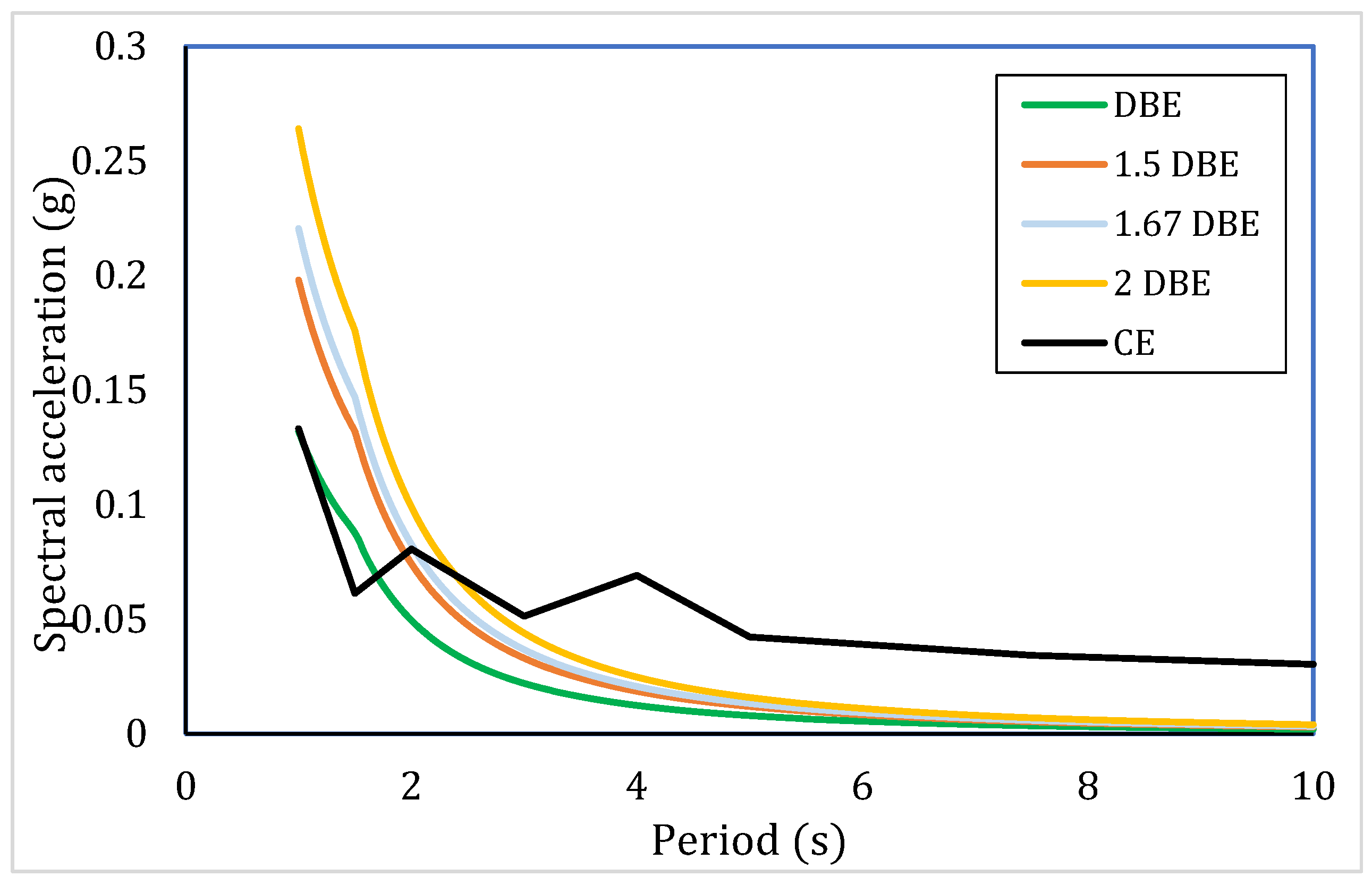
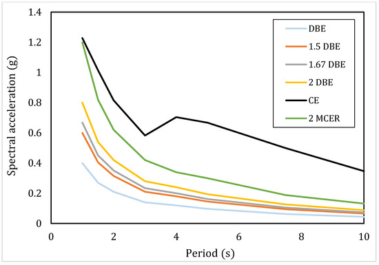
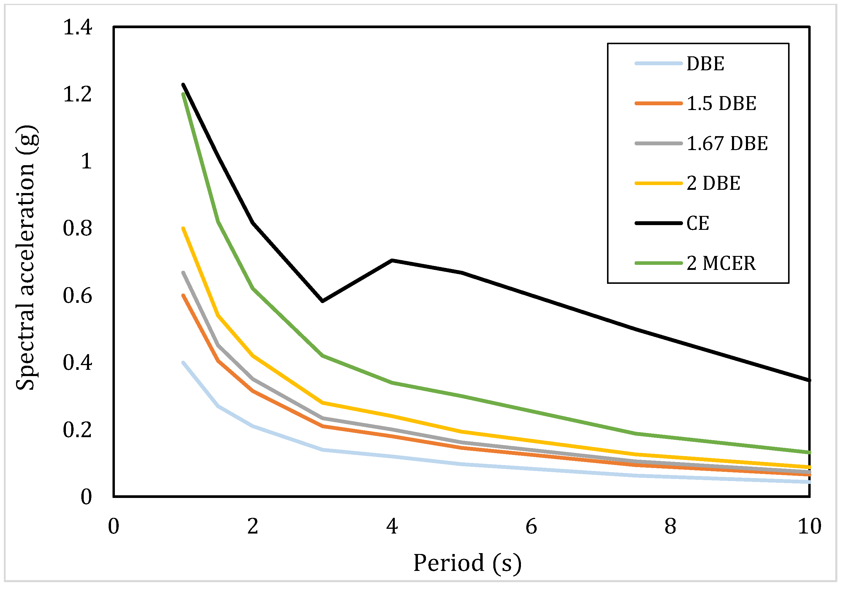

Disclaimer/Publisher’s Note: The statements, opinions and data contained in all publications are solely those of the individual author(s) and contributor(s) and not of MDPI and/or the editor(s). MDPI and/or the editor(s) disclaim responsibility for any injury to people or property resulting from any ideas, methods, instructions or products referred to in the content. |
© 2026 by the authors. Licensee MDPI, Basel, Switzerland. This article is an open access article distributed under the terms and conditions of the Creative Commons Attribution (CC BY) license.