Estimation of the Elastic Modulus of Granite Under Uniaxial Compression at the Pre-Peak Stage Using the PROS Method for Approximating Experimental Data

Abstract

This study investigates the application of the Pure Random Orthogonal Search (PROS) method, introduced in the literature in 2021, for approximating force and displacement measurement data obtained from rock specimen testing, using granite as a case study. The primary objective is to simplify the data approximation procedure and improve the accuracy of experimental data analysis by reducing the influence of subjective factors within a predefined protocol. The research focuses on determining the maximum value of the tangent modulus of elasticity during the pre-peak deformation stage of granite specimens under uniaxial compression. The study employs methods of mathematical modeling of rock mechanical behavior and experimental data analysis. To approximate the experimental data, a modified two-parameter S-curve equation is proposed. The optimal parameter values are determined using the PROS method, which reduces the problem to solving a two-dimensional objective function minimization task. The dimensionality of this optimization problem remains independent of the number of experimental data points, thereby enhancing computational efficiency. A systematic computational procedure is developed for the automated calculation of the approximating equation’s parameters and the determination of the maximum tangent modulus of elasticity. In the context of challenges associated with accurately measuring displacements using conventional testing machines, a numerical correction procedure is proposed and implemented to account for the compliance of the loading system. The results of the study are consistent with both the literature-reported experimental data and the data obtained in this work. The methodology and findings can be adapted for analyzing the properties of concrete as an artificial analog of natural rock materials.

1. Introduction

1.1. Research Problem

This article proposes a methodology for approximating experimental data, which allows reducing the influence of subjective factors when determining the modulus of elasticity of rocks under uniaxial compression. A generally accepted method for presenting the results of axial compression tests of rocks, both with and without lateral pressure, is stress–strain curves obtained after processing the measurement results, which initially represent a set of points in load–displacement coordinates. Stress–strain curves, in combination with other dependencies, are necessary for determining the key mechanical properties used in the process of modeling and analyzing the behavior of rocks [1,2,3]. The conditions of the origins of rocks and their subsequent history are such that they contain micro-, meso- and macro-cracks, while maintaining a certain strength. However, if natural or manufactured impacts increase and reach certain threshold values, new cracks appear, which reduces the strength of the rock. Accordingly, the risk of failure of a natural or artificial structure in which rock serves as the load-bearing material increases. Consequently, the problem of predicting the threshold stress for crack initiation arises [4,5]. This threshold value corresponds to a specific point on the stress–strain curve. To determine sufficiently accurate values of the threshold stress for crack initiation, it is necessary to consider the process of the deformation and failure of the rock.

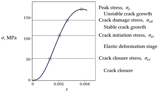
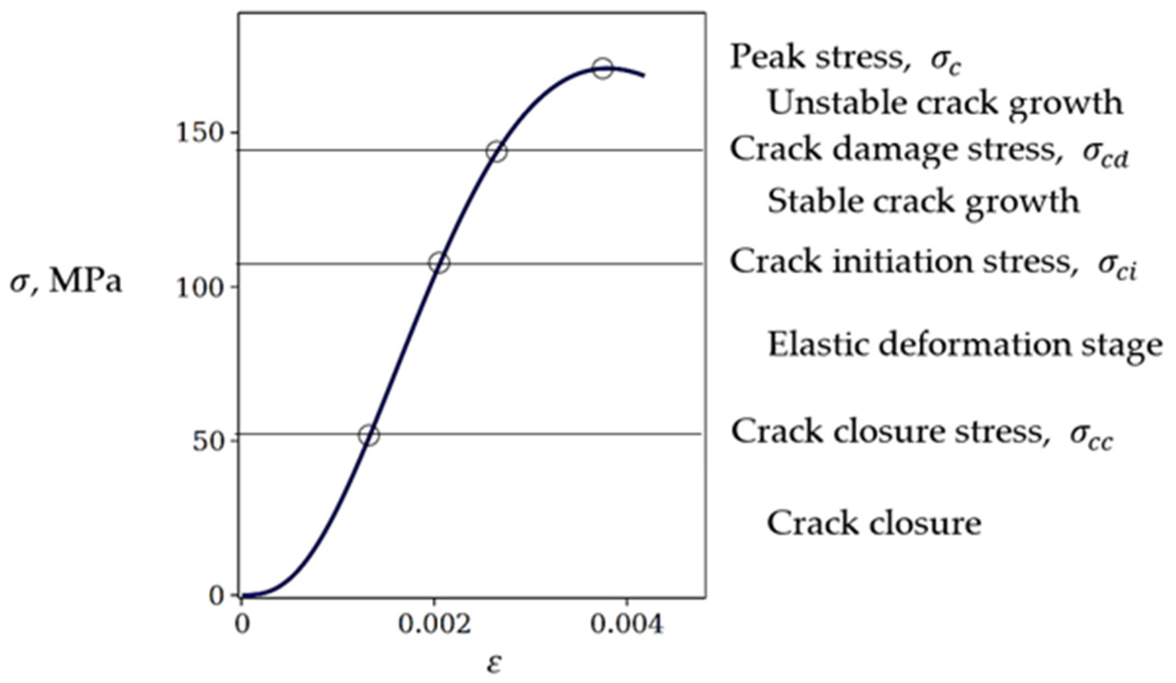
Numerous tests of rock specimens for uniaxial compression, including those taking into account lateral pressure, have shown that the process of their deformation and destruction can be divided into several stages [6,7,8]. These stages and threshold stress values correspond to the following sections and points on the stress–strain curve (Figure 1): (1) crack closure and crack closure stress; (2) elastic region and crack initiation stress; (3) stable crack growth and crack damage stress; (4) unstable crack growth and peak stress (5) failure and post-peak behavior.

Figure 1. Deformation stages and stress thresholds.

Determining the peak stress value is relatively straightforward, as the corresponding point (Figure 1) is typically unambiguously identifiable from the experimental data. However, the identification of other threshold stress values requires more careful analysis.

Eberhardt et al. [7] established that the crack damage stress corresponds to the stress level at which the relative volumetric strain reaches its maximum. The use of this criterion effectively reduces the influence of subjective factors when determining the threshold level of stress. The validity of this approach has been further supported by acoustic emission measurements reported by Zhao et al. [9].

Determining the crack initiation (CI) stress presents a more complex challenge. To improve the accuracy of estimates and deepen the understanding of rock deformation and failure mechanisms, it is advisable to combine the acoustic emission method with complementary techniques.

To enable consistent comparison of crack initiation stress across different rock types, numerous studies have examined the ratio of crack initiation stress to peak stress under uniaxial compression (CI/UCS). Nicksiar and Martin [10] applied a statistical approach to analyse test results from 376 specimens of igneous, sedimentary, and metamorphic rocks. They found that:

• Under unconfined uniaxial compression, CI/UCS ranges from 0.42 to 0.47, regardless of material properties;
• Under constrained compression, this ratio increases to 0.50–0.54.

Generalized estimates of crack initiation and failure stresses for brittle rock masses near underground workings were developed by Cai et al. [11,12].

Using group theory to model rock damage, Yan et al. [5] derived a theoretical expression for CI/UCS in brittle rocks, reporting a range of 0.43–0.52. However, the authors note that for rocks with properties significantly differing from those considered in their study, it is essential to first evaluate material heterogeneity to assess the applicability of this CI/UCS range. This observation highlights the existing gaps and underscores the need for more universal methods of determining CI/UCS values.

Addressing the practical significance of this issue, Dong et al. [13] investigated the applied aspects of crack nucleation and propagation. They employed numerical simulations of freeze induced crack propagation in fractured rocks during water–ice phase transition using the discrete element method [14].

In a related study, Li et al. [15] developed a model for determining the strength and failure behavior of rock unit cells under uniaxial compression. Their approach combined phenomenological theory and fracture mechanics principles.

Lin et al. [16] investigated crack closure stress and crack initiation stress in fractured rocks using stress–strain curve analysis. Similarly, Qiang et al. [17] explored alternative approaches to improve the accuracy of crack initiation stress determination by minimizing the influence of subjective factors.

Both studies [16,17] emphasize the importance of reducing subjectivity in data interpretation, particularly for parameters sensitive to small deviations in experimental data—such as the tangent modulus and threshold stress values. While employing multiple methods [16] helps mitigate the influence of subjectivity, it does not fully eliminate it.

For instance, when using the acoustic emission method to study rock deformation stages, reliable data acquisition requires accounting for external noise interference, the structural and mineralogical characteristics of the rock, and the potential manifestations of prior stress history (as described by the Kaiser effect) [18,19,20]. These factors contribute to the inherent uniqueness of each specimen [21]. Consequently, while complete elimination of subjective influence may not be feasible, its impact can be progressively reduced through the development of novel approaches, methods, and algorithms. The present study contributes to this ongoing effort.

Methods for determining the rock tangent modulus are closely related to this challenge. Briševac et al. [22] demonstrated that if stress and strain values at characteristic points are known (see Figure 1), the tangent modulus E can be calculated using Equation (1):

$$E={\displaystyle \frac{{\sigma }_{cd}-{\sigma }_{ci}}{{\epsilon }_{cd}-{\epsilon }_{ci}}} .$$

(1)

Analysis of the stress–strain curve—constructed from uniaxial compression test results on a rock specimen—enables the determination of key mechanical parameters, including crack closure stress (${\sigma }_{cd}$), crack initiation stress (${\sigma }_{ci}$), and tangent modulus (E), as defined by Equation (1). However, experimental data acquired from testing equipment are typically recorded as a discrete set of measurement points, either in the stress–strain or stress–time coordinate system. The temporal resolution (i.e., data acquisition interval) may be as fine as 0.01 s. Consequently, to generate a continuous stress–strain curve that is comparable to the idealized representation shown in Figure 1, it is necessary to apply an approximation procedure. This involves one of the following approaches:

• Fitting the discrete dataset with an appropriate mathematical function that captures the underlying mechanical behavior of the material.
• Constructing a smooth approximating curve that accurately represents the physical response of the rock across the full range of deformation stages.

Such approximation is essential for reliably identifying characteristic points on the curve and for computing derived mechanical properties with minimal subjectivity in data interpretation.

1.2. Approximation

Approximation refers to the process of developing a mathematical model that reproduces the mechanical behavior of rock with minimal deviation from the experimental data. Such a model typically comprises one or more approximating equations designed to simulate the stress–strain relationship—for instance, across both the pre-peak and post-peak stages of deformation. To address the problem of minimizing deviations between the model and experimental observations, optimization methods (i.e., techniques for finding function minima) are employed. Approximation offers several key advantages in geotechnical data analysis [23], including smoothing out noise and measurement errors in experimental data; reducing the volume of analyzed information without significant loss of accuracy in geotechnical assessments; simplifying calculations during test data processing; enabling extrapolation of data beyond the observed range; identifying characteristic points on the stress–strain curve, as well as key trends and patterns.

The least-squares method is currently one of the most widely used approaches for determining the parameters of approximating equations [24,25,26]. However, this method is not always numerically stable. For example, instability in solving an applied problem in compression testing is reported in [27], where the analysis produced unacceptable results—likely due to a limited dataset concentrated within a narrow stress or strain range.

In addition to the least-squares method, alternative techniques are employed for parameter estimation when experimental data exhibit outliers, anomalous error distributions, or heteroscedasticity [28,29]. However, such methods do not always achieve an acceptable balance between algorithmic complexity, versatility, and the accuracy of numerical results. This limitation can be addressed by employing an appropriate variant of the random search method.

Random search methods are known for their high versatility and broad applicability. Nevertheless, their widespread use has historically been limited by slow convergence to the optimal solution. This drawback was significantly mitigated with the introduction of the parameter-free orthogonal random search (PROS) method in 2021 [30], which offers improved convergence properties while maintaining robustness in handling noisy or sparse datasets. When combined with a newly modified version of the S-curve equation [31] derived from the Blagojević model (first introduced in [32]), the PROS method demonstrates high effectiveness as an approximation tool.

The objective of this study is to simplify the data approximation procedure and improve the accuracy of experimental data analysis by reducing the influence of subjective factors within a predefined protocol. The research focuses on determining the maximum value of the tangent modulus of elasticity during the pre-peak deformation stage of granite specimens under uniaxial compression. This requires sufficiently accurate experimental data. In the context of the problems associated with accurately determining displacements using conventional testing machines when plotting load–displacement curves, the possibility of numerical correction of the measured displacements is investigated.

2. Methodology

2.1. Approximation of Experimental Data

2.1.1. Approximating Equation

To approximate the experimental data in this study, a modified S-curve equation [31] with two dimensionless parameters, n and B (Equation (2)), is employed. The values of these parameters are determined using the PROS method:

$$\begin{gathered} \sigma ={\sigma }_c{\left({\displaystyle \frac{\epsilon }{{\epsilon }_c}} \mathrm{e}\mathrm{x}\mathrm{p}\left( {\displaystyle \frac{T}{n}} \right)\right)}^B, \\ T=\left(1-{\left({\displaystyle \frac{\epsilon }{{\epsilon }_c}}\right)}^n\right) \end{gathered}$$

(2)

The parameters ${\sigma }_c$ and ${\epsilon }_c$, which correspond to the peak point (see Figure 1), are determined experimentally and included in the initial dataset. These values remain constant throughout the approximation process.

The following section details the application of the PROS method for calculating the parameters n and B.

2.1.2. Procedure of Approximation

If no prior experimental data are available (e.g., from the literature sources), the specimen is tested to failure. During the test, displacement and load (force) are recorded at regular time intervals—for instance, every 0.01 s—and subsequently converted into strain (ε) and stress (σ), respectively. The measured strain and stress values are henceforth denoted as $\overline{\epsilon }$ and $\overline{\sigma }$, with appropriate subscripts to indicate specific data points.

In the problem under consideration, the initial data must include the following:

• The measured stress value at the peak point (${\overline{\sigma }}_c, {\overline{\epsilon }}_c$);
• Measured strain values ${\overline{\epsilon }}_i$ at several intermediate points $0 {<\overline{\epsilon }}_i<{\overline{\epsilon }}_c$, $i=1, 2,\dots ,m,$ $m_{lb}<m\le m_{ub}$; the lower ($m_{lb})$ and upper ($m_{ub})$ boundaries of the number $m$ are determined empirically, for example, $m_{lb}=4, m_{ub}=10$ for granite.

These data are represented as a set of pairs:

$${\overline{\sigma }}_0, {\overline{\epsilon }}_0; {\overline{\sigma }}_1, {\overline{\epsilon }}_1;\dots , {\overline{\sigma }}_m, {\overline{\epsilon }}_m; {\overline{\sigma }}_c, {\overline{\epsilon }}_c.$$

(3)

Here ${\overline{\sigma }}_0=0$, ${\overline{\epsilon }}_0=0$. The above number of intermediate points m is determined empirically; in this study, m = 4. The curvature of the approximated curve sections depends on the mechanical properties of the specific rock type. Generally, the greater the curvature of a section is, the more points are required to accurately represent it. A separate investigation is needed to develop precise recommendations for different rock types.

The PROS algorithm identifies values of the parameters n and B that minimize the discrepancy between the calculated stress values ${\sigma }_i$ (from Equation (2)) and the measured stress values ${\overline{\sigma }}_i$, where i = 1, …, m.

The accuracy of the approximation is evaluated using the objective function $f_{ob}$, defined as follows:

$${f_{ob}=f_1+f_2+\dots +f_m,}_0.$$

(4)

where

$$f_i={\left({\sigma }_i-{\overline{\sigma }}_i\right)}^2,i=1, \dots , m.$$

Here, ${\sigma }_i$ and ${\overline{\sigma }}_i$ denote the above stress values calculated by Equation (2) and measured during the tests respectively.

The PROS algorithm solves the minimization problem for $f_{ob}$, where the independent variables are the parameters n and B. The optimal values of n and B, which yield the minimum (ideally zero) value of $f_{ob}$, constitute the solution to the problem. Thus, determining the parameters n and B of the approximating equation (Equation (2)) reduces to minimizing a two-dimensional objective function, regardless of the number of above experimental points m.

The upper and lower boundaries of the range of possible values of the parameters n and B are established empirically. For granite, typical bounds are $1\le n\le 50$ and $1\le B\le 50.$

Using Equation (2) and the selected ${\overline{\epsilon }}_i$ for i = 1,…, m, compute the predicted stress values ${\sigma }_i$. The points (${\overline{\epsilon }}_i$, σ_i) lie on the approximating curve.

Compute residuals: Calculate $f_i={\left({\sigma }_i-{\overline{\sigma }}_i\right)}^2$ for each i = 1,…, m.

Evaluate the objective function: Compute $f_{ob}$ (4) as the sum of all $f_i$.

Optimize using PROS: Search for the minimum of $f_{ob}$ using the PROS algorithm [30].

As the above number of intermediate points specified in the experimental dataset (3) increases, the approximation accuracy increases up to a certain limit, which is typical for numerical methods. A reasonable limit for the number of intermediate points can be determined empirically (through trial calculations). Uniform distribution of these points is not mandatory, but is preferred when selecting them automatically. In the future, an additional algorithm integrated into the measurement results processing program will be able to automatically select specified points without user intervention, mitigating the influence of subjective factors on the results of the geotechnical analysis.

Regardless of the number of intermediate points, the search is performed using the PROS algorithm in a two-dimensional domain with upper and lower bounds for the parameters $n$ and $B$, respectively: $n_{lb}\le n\le n_{ub}$ and $B_{lb}\le B\le B_{ub}$. These boundaries are established empirically, based on experience in solving similar problems and research objectives.

According to the PROS algorithm [30], only one of the parameters (n or B) changes during the solution process. If a change in parameter n decreases the value of the objective function (4), then the search continues from the found position in the same direction n. If a change in parameter n increases the value of the objective function, then a transition to the search in the orthogonal direction B is performed. If the value of the objective function increases, then a transition to the search in the direction n is performed, and so on.

The iterations are terminated based on the maximum number of attempts or the accuracy of the result. The approximation methodology is illustrated by the following example.

2.1.3. Example 1. Determining the Parameters of the Approximating Equation

Let us consider the pre-peak stage of the deformation of granite, the experimental data for which were obtained from the stress–strain curve, which, along with other results, was obtained using digital image correlation (DIC) in the study of Aboayanah et al. [33]. The experimental data are represented by the stress and strain values at the initial and peak points, as well as at four intermediate points (Table 1). In this example, m = 4.

Table 1. Experimental data *.

${\overline{\mathit{\sigma }}}_0$	${\overline{\mathit{\epsilon }}}_0$	${\overline{\mathit{\sigma }}}_1$	${\overline{\mathit{\epsilon }}}_1$	${\overline{\mathit{\sigma }}}_2$	${\overline{\mathit{\epsilon }}}_2$	${\overline{\mathit{\sigma }}}_3$	${\overline{\mathit{\epsilon }}}_3$	${\overline{\mathit{\sigma }}}_4$	${\overline{\mathit{\epsilon }}}_4$	${\overline{\mathit{\sigma }}}_{\mathit{c}}$	${\overline{\mathit{\epsilon }}}_{\mathit{c}}$
0	0	23.8	0.00086	67.5	0.001925	107.4	0.00267	147.4	0.003415	170.8	0.00399

* Stress values are given in MPa.

Based on experience solving similar problems, we establish approximate bounds for the possible values of the parameters n and B: $1\le n\le 50$; $1\le B\le 50$.

Generate a pair of random numbers to initialize the initial values of the parameters, for example, $n=$ 2.909 and $B=$ 20.806. These are the starting values of parameters n and B.

The value of ε is initialized to a random number (${\overline{\epsilon }}_0\le \epsilon \le {\overline{\epsilon }}_c$). The stress is calculated using Equation (2).

Thus, the initial values n, B, ε, σ are determined, which are necessary to start calculations using the PROS algorithm [30].

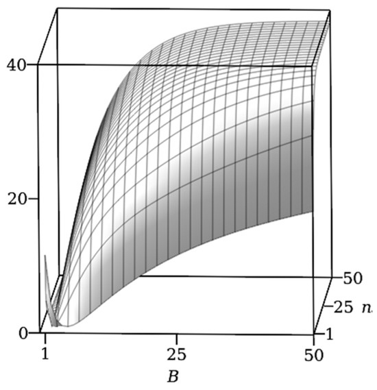
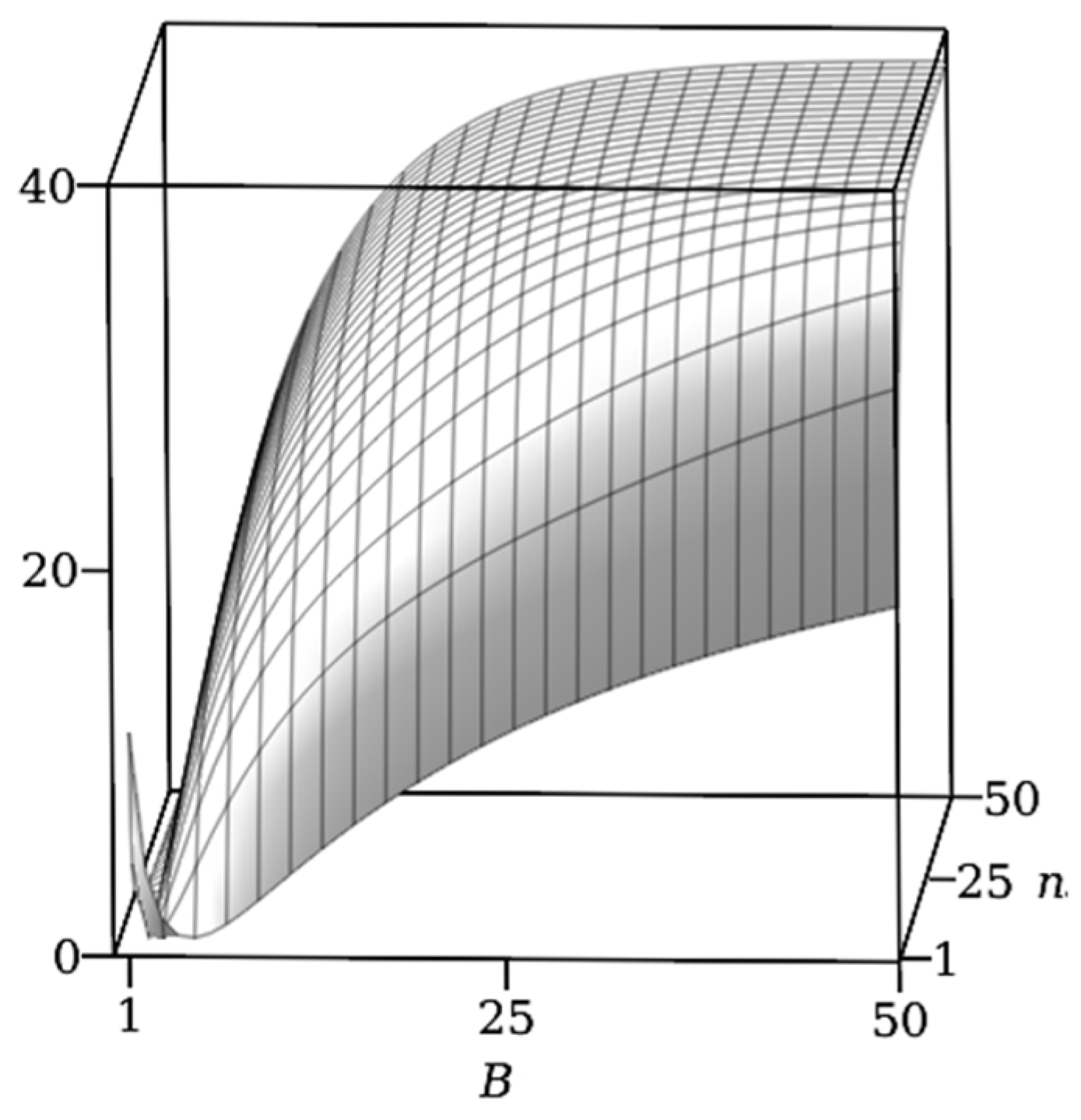
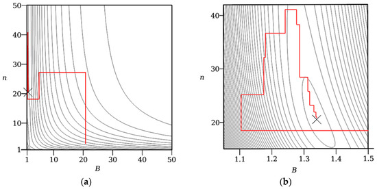
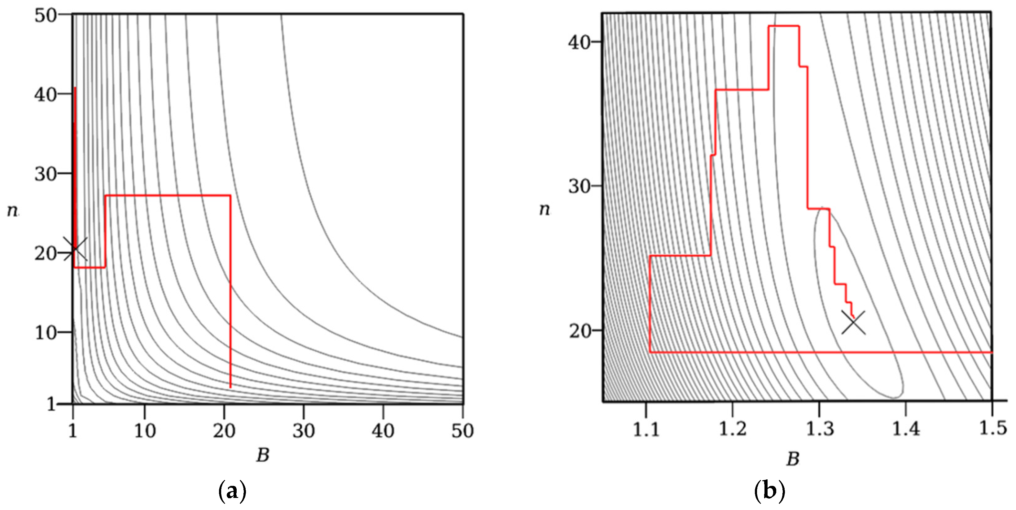
Figure 2 shows the plot of the objective function (4). Figure 3 shows the general view and details of the trajectory to the goal using the aforementioned PROS algorithm.

Figure 2. Plot of the objective function. The minimum point is on the left side, in the “ravine”.

Figure 3. The trajectory of movement to the target according to the PROS algorithm. (a) The algorithm starts from the point with coordinates B = 20.807, n = 2.909. The minimum point (×) is on the left side of the plot, in the “ravine” (B = 1.3398, n = 20.4523). (b) Detailing the trajectory in the vicinity of the minimum point.

The results (Figure 3) reflect the path to the target and the accuracy of the PROS algorithm. The trajectory detail in the range $1.05\le B\le 1.5$ (Figure 3b) demonstrates automatic step reduction and elegance as the target is approached. In this example, the PROS algorithm yields parameter values n = 20.4523 and B = 1.3398, which are necessary for calculations using Equation (2).

Despite the limited number of tests conducted, the following advantages of the considered approach to determining the parameters n and B using the PROS algorithm deserve further study:

• The parameters were determined using only the measurement results (Table 1) and Equation (2), without any additional parameters.
• The search for the values of the parameters $n$ and $B$ of the approximating Equation (2) is reduced to solving the problem of minimizing the two-dimensional objective function $f_{ob}$ (4), regardless of the number of experimental points.
• The procedure for determining the parameters n and B (2) can be performed automatically, without user intervention, to mitigate the influence of subjective factors on the accuracy of the analysis results.

2.1.4. Example 2: Approximation

This example is based on the same experimental data from [33] as Example 1 discussed above.

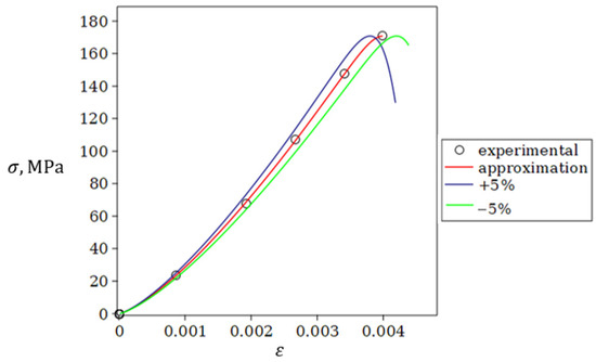
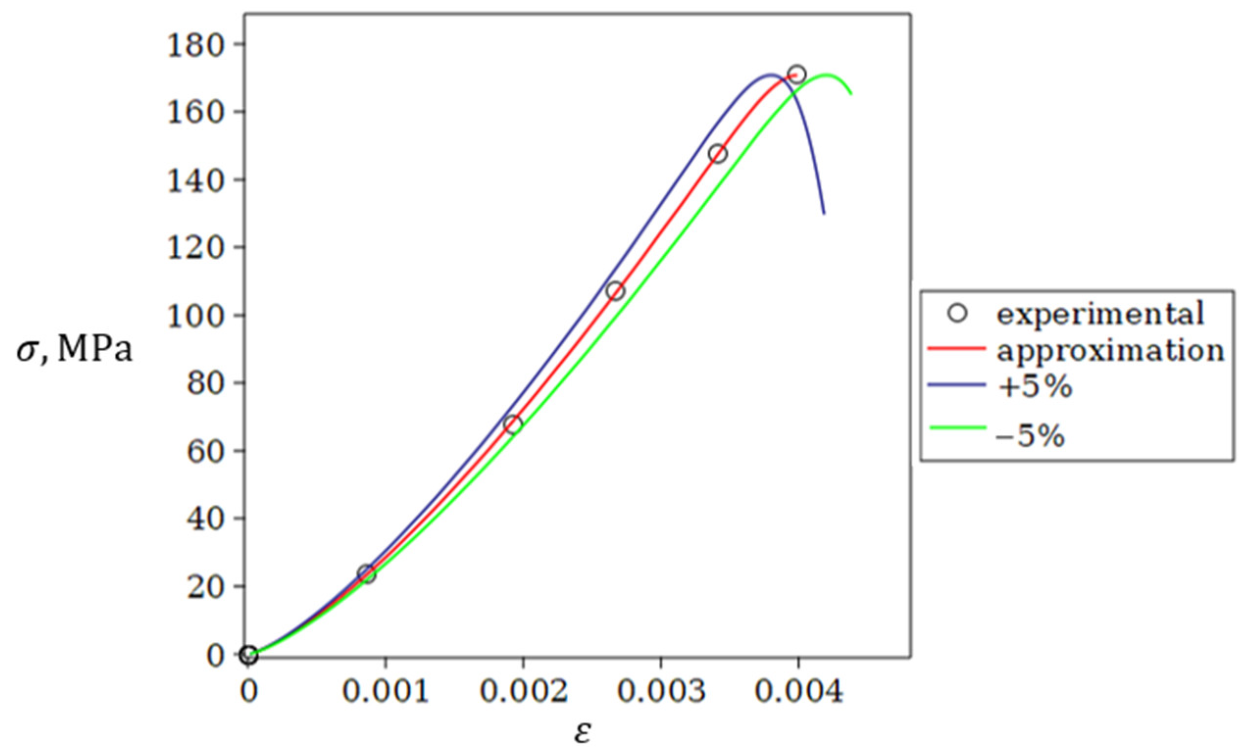
Using the found values of $n$ and $B$ (Figure 3), as well as the experimental values of ${\overline{\epsilon }}_c$ and ${\overline{\sigma }}_c$ (Table 1), we specify Equation (2), which in the example under consideration takes the following form (5):

$$\sigma =170.8{\left({\displaystyle \frac{\epsilon }{0.00399}} \mathrm{e}\mathrm{x}\mathrm{p}\left({\displaystyle \frac{1}{20.4523}}\left(1-{\left({\displaystyle \frac{\epsilon }{0.00399}}\right)}^{20.4523}\right)\right)\right)}^{1.3398}.$$

(5)

Figure 4 shows the experimental data (circles) from Table 1 and the fitting curve (5).

Figure 4. Experimental data (circles) and fitting curve (red). The limits for $\sigma$ are shown if the experimental strain values $\epsilon$ for stress calculations according to Equation (5) are determined with deviations of +5% (navy) and −5% (green) from the experimental values $\epsilon$.

Figure 4 shows that Equation (5) approximates the experimental data at the pre-peak stage of deformation quite accurately; small deviations are due to the inevitable influence of rounding of numbers. The high accuracy of the approximation allows the use of the approximating Equation (5) to determine the modulus of elasticity by differentiation, as shown in the following section.

2.2. Determination of the Maximum Pre-Peak Tangent Modulus

2.2.1. Necessary Clarifications

From a physical point of view, the modulus of elasticity is a characteristic of the rigidity of a material. From a geometric point of view, the modulus of elasticity is numerically equal to the tangent of the angle of inclination of the tangent to the stress–strain curve. The less fracturing a rock has, the higher its rigidity is.

At the first stage of deformation (Figure 1), with increasing load, the proportion of the work of external forces spent on closing cracks gradually decreases, and, accordingly, the proportion of work spent on deforming mineral grains, their conglomerates and the bonds between them increases. A small number of the weakest particles and particle contacts can be destroyed, which is confirmed by acoustic emission measurements [18]. The crack faces converge and close, the rock compacts, the rigidity increases and at a certain point in the second stage (Figure 1) reaches a maximum. At this point, the curvature changes sign; on the stress–strain curve, the downward convexity disappears (the tangent slope ceases to increase) and an upward convexity appears (the tangent slope decreases).

From a physical perspective, the change in sign of the curvature means that after passing its maximum point, the tangent modulus decreases, which is only possible with the appearance of new cracks, the destruction, and the loss of the weakest (or most highly loaded) grains, their conglomerates, and the material connecting them. It is logical to assume that at this point in the second stage (Figure 1), all cracks are closed, so the rock density is maximum, and the tangent modulus will approximately correspond to the tangent modulus of intact rock. Accordingly, the mechanical behavior of the rock in this state is analogous to the behavior of an ideal elastic material, described by Hooke’s law. Strictly speaking, this state corresponds to only one point on the stress–strain curve, the search procedure for which can be formalized, i.e., can be performed without the influence of subjective factors if a sufficiently accurate approximating equation is known (in the example under consideration, this is Equation (5)).

From a mathematical point of view, the tangent modulus of elasticity is numerically equal to the first derivative of function (2) (or function (5) for the example under consideration):

$$E={\displaystyle \frac{d\sigma \left(\epsilon \right)}{d\epsilon }}$$

(6)

Using Equation (2), we obtain after the transformations:

$$\begin{gathered} E=B{\sigma }_c{\left({\displaystyle \frac{\epsilon }{{\epsilon }_c}} \mathrm{e}\mathrm{x}\mathrm{p}\left( {\displaystyle \frac{T}{n}} \right)\right)}^B {\displaystyle \frac{T}{\epsilon }} , \\ T=\left(1-{\left({\displaystyle \frac{\epsilon }{{\epsilon }_c}}\right)}^n\right) \end{gathered}$$

(7)

The pre-peak branch model is an S-shaped curve with an inflection point (Figure 1). At this point, the tangential tangent modulus (7) reaches a maximum and begins to decrease to zero at the peak point. The value $\epsilon ={\epsilon }_E$, at which the tangent modulus (7) reaches a maximum, can be found by solving the following Equation (8):

$${\displaystyle \frac{dE\left(\epsilon \right)}{d\epsilon }}={\displaystyle \frac{d^2\sigma \left(\epsilon \right)}{{d\epsilon }^2}}=0$$

(8)

Substituting Equation (2) into Equation (8) after transformations, we can determine the deformation at which the modulus of elasticity reaches its maximum (9) [31]:

$${\epsilon }_E={\epsilon }_c{\left(1+{\displaystyle \frac{n-1-\sqrt{4Bn+{(n-1)}^2}}{2B}} \right)}^{{\displaystyle \frac{1}{n}}}$$

(9)

The stress ${\sigma }_E$ at which the tangent modulus reaches its maximum is determined by Equation (2) after substituting $\epsilon ={\epsilon }_E$ from Equation (9). The maximum pre-peak tangent modulus is determined by Equation (7) after substituting the value $\epsilon ={\epsilon }_E$ (9).

2.2.2. Example 3. Pre-Peak Tangent Modulus

This example is based on the same experimental data from [33] as Examples 1 and 2 discussed above.

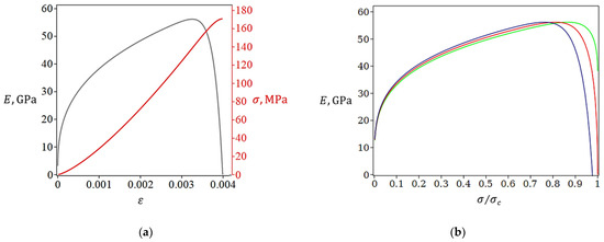
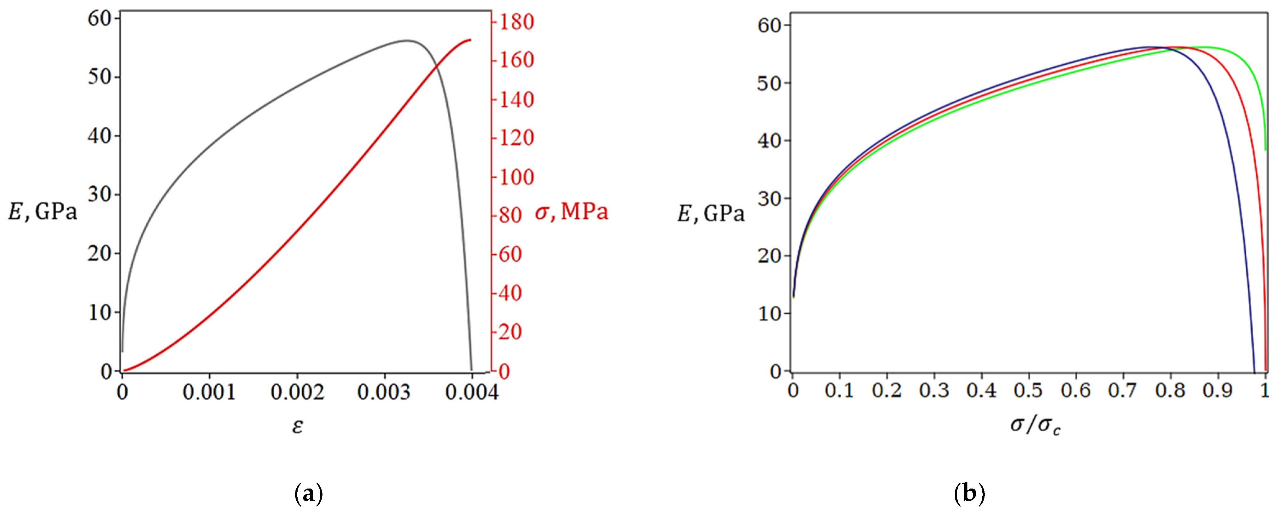
By substituting the numerical values of ${\sigma }_c$ ${\epsilon }_c$, $n$, and $B$ defined above (Section 2.1.3) into Equation (7), one can calculate the value of the tangent modulus for any value of $\epsilon$ in the pre-peak stage ($0<\epsilon \le {\epsilon }_c$). Figure 5 shows the plots of the functions $E \left(\epsilon \right)$ and $\sigma \left(\epsilon \right)$ for the example under consideration. The initial data and results of calculating the modulus of elasticity are given in Table 2.

Figure 5. (a) Dependences of stress $\sigma \left(\epsilon \right)$ (red) and tangential tangent modulus $E\left(\epsilon \right)$ (gray) on axial strain. (b) Dependence of tangential tangent modulus on normalized stress ($E\left(\sigma /{\sigma }_c\right)$), if experimental values of strain $\epsilon$ for calculating stress $\sigma$ according to Equation (5) were determined with deviations of +5% (dark blue), 0% (red) and −5% (green) from the experimental values of $\epsilon$.

Table 2. Initial data and calculation results.

$\mathit{n}$	$\mathit{B}$	${\mathit{\epsilon }}_{\mathit{c}}$	${\mathit{\sigma }}_{\mathit{c}}$(MPa)	${\mathit{\epsilon }}_{\mathit{E}}$	${\mathit{\epsilon }}_{\mathit{E}}/{\mathit{\epsilon }}_{\mathit{c}}$	${\mathit{\sigma }}_{\mathit{E}}$(MPa)	${\mathit{\sigma }}_{\mathit{E}}/{\mathit{\sigma }}_{\mathit{c}}$	$\mathit{E}$(GPa)	$\mathit{E}/{\mathit{\sigma }}_{\mathit{c}}$
20.452	1.339	0.00390	170.8	$0.00325$	0.833	138.6	0.811	56.20	329.0

For the example under consideration, the values of the tangent modulus are known from the literature; they were experimentally determined in two ways on the region of the stress–strain curve with boundaries of 0.45${\sigma }_c$ and 0.55${\sigma }_c$. Using the first method (sensors), a value of 52.57 GPa was obtained, and using the second method (digital image correlation), a value of 51.79 GPa was obtained in [33].

For comparison, the proposed method yields a tangent modulus of elasticity value of 51.84 GPa at a stress level of 0.55σ_c. The tangent modulus reaches its maximum value of 56.2 GPa at the point with coordinates ε = 0.00325, σ = 138.6 MPa (Table 2).

As noted above, the elastic modulus can be calculated using Equation (1), which is analogous to the equation $E={\displaystyle \frac{{\sigma }_u-{\sigma }_l}{{\epsilon }_u-{\epsilon }_l}}$. It should be noted that the modulus calculated using this formula may be referred to as the chord modulus of elasticity. This term reflects the geometric aspects of the problem by an analogy with the terms “tangent modulus of elasticity” and “secant modulus of elasticity”.

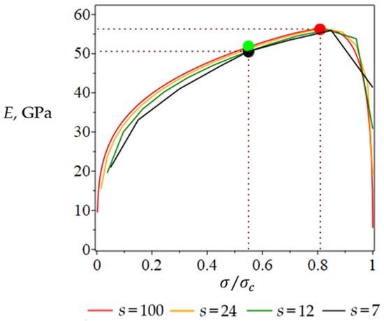
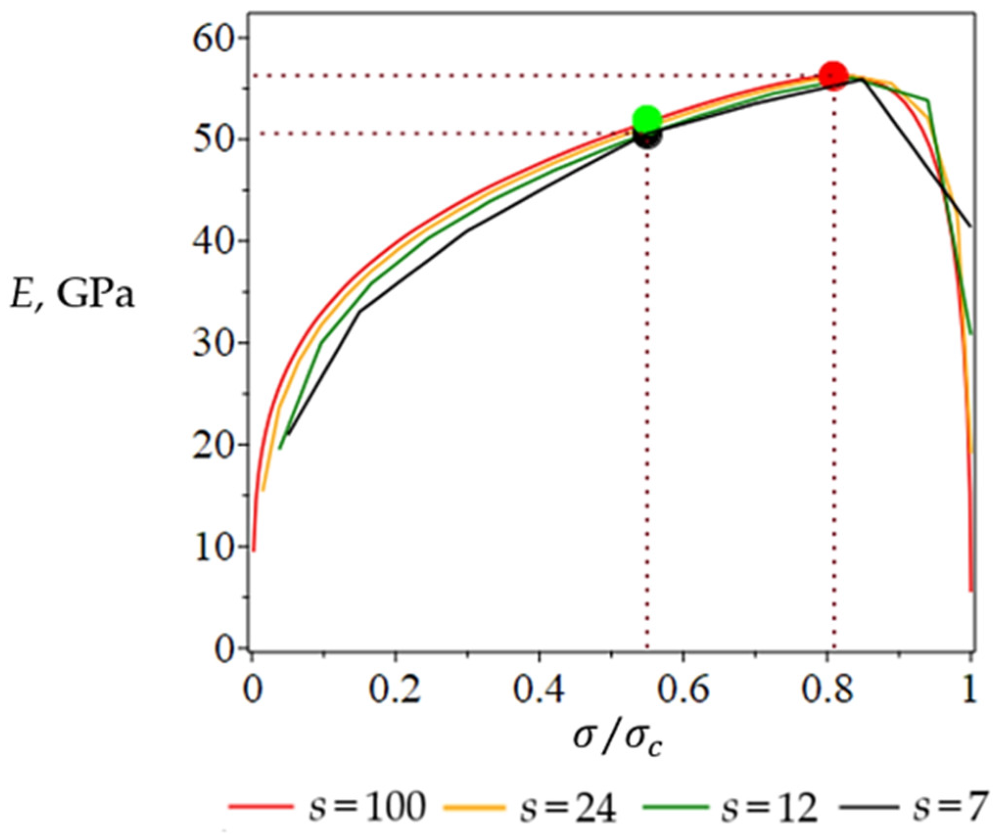
For comparison, Figure 6 presents the results of chord modulus calculations in graphical form, assuming that the stress–strain curve is divided into s segments. The black point corresponds to the chord modulus value of 51.79 GPa at a stress level of 0.55${\sigma }_c$; the green point corresponds to the tangent modulus of elasticity (51.84 GPa) obtained using the proposed method at the same stress level. The red point in Figure 6 indicates the maximum value of the tangent modulus of elasticity (56.2 GPa). As the number of segments increases, the modulus values obtained using the considered methods converge, which confirms the reliability of the results.

Figure 6. Convergence of the elastic modulus values obtained using the discussed methods (explanations provided in the text above).

2.3. Linear-Elastic Stage of Rock Deformation

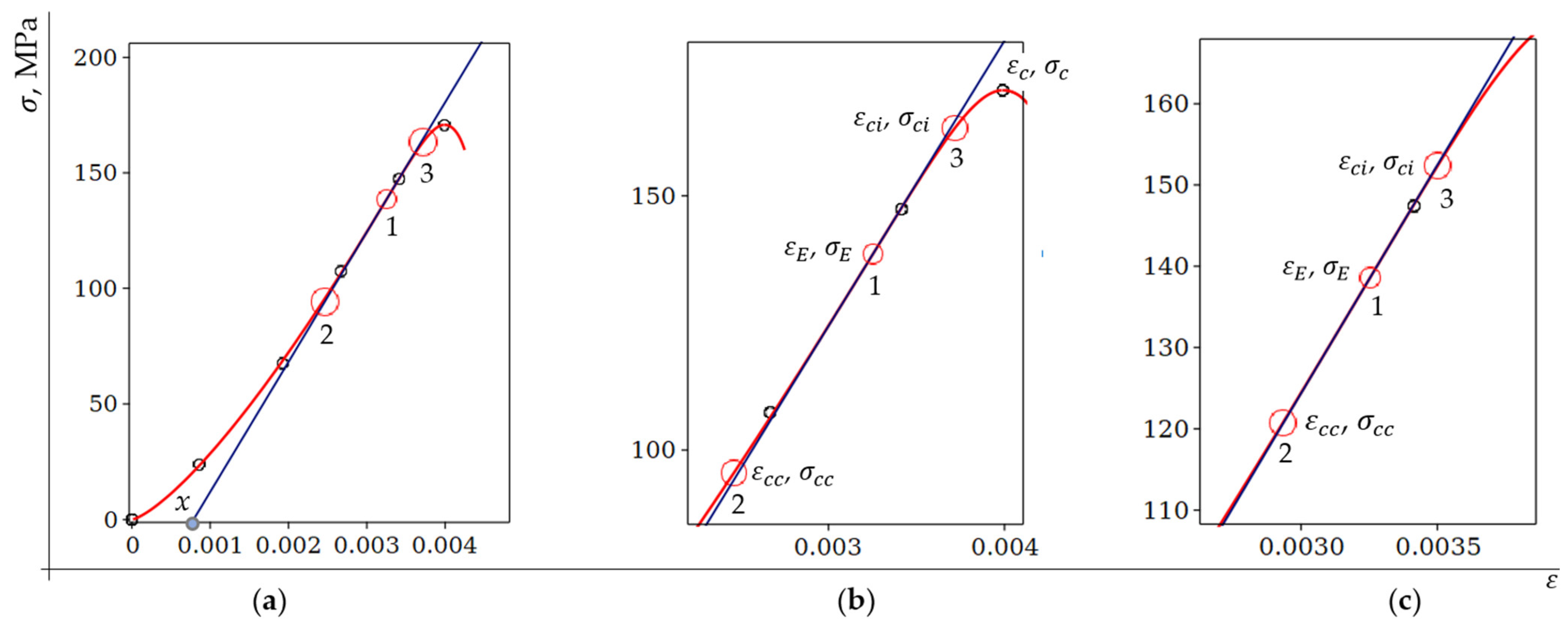
The analysis in Section 2.2 showed that at the point for which condition (8) is satisfied, the tangent modulus is maximum, which indirectly confirms crack closure. Therefore, this point is a candidate for determining the crack closure stress (${\sigma }_{cc}$, Figure 1).

However, as described in detail above (Section 2.2.1), after passing this point on the stress–strain curve, the tangent modulus decreases to zero at the peak stress and becomes negative at the post-peak stage. This is only possible with the appearance of new cracks, partial failure, and deactivation of the weakest grains, their conglomerates, and the material connecting them (this mechanical behavior is demonstrated in rock specimens under uniaxial compression). Therefore, this point is a candidate for determining the initiation stress of new cracks.

Thus, formally, the point at which condition (8) is satisfied defines the boundary between the stage of existing crack closure and the stage of new crack formation. However, a certain region of the stress–strain curve is visually perceived as a straight-line segment, characteristic of the linear-elastic stage of deformation, as shown generally in Figure 1 and illustrated in more detail in Figure 7.

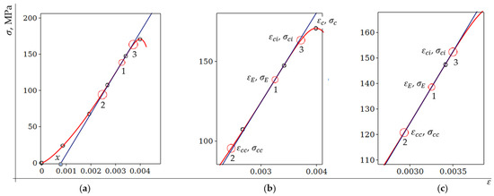
Figure 7. (a) Experimental points (small circles), the approximating curve, and the tangent passing through inflection point 1 (at point 1 the curvature changes sign, the downward convexity disappears and an upward convexity appears). Points 2 and 3 are determined using Equation (5) under the condition that the difference in the ordinates of the tangent and the approximating curve at points 2 and 3 is equal to 1% of the stress at point 1 ($∆\sigma =0.01{\sigma }_E$). The tangent intersects the abscissa axis at point $x=$0.0007873. (b) Fragment of the plot if $∆\sigma =0.01{\sigma }_E$. (c) Fragment of the plot if $∆\sigma =0.001{\sigma }_E$.

Figure 7 shows that the tangent at point 1, for which condition (8) is satisfied, almost coincides with the curve in Section 2 and Section 3. Reducing the difference in the ordinates of the tangent and the approximating curve at points 2 and 3 from 1% of the stress at point 1 to 0.1% reduced the length of the section of nearly linear deformation.

Obviously, any point in regions 2–3 can be selected as a criterion. This feature is the objective reason for the existence of subjective factors and their influence on the results of geotechnical analysis. Therefore, the use of automated processing of experimental data is necessary to improve the reliability of calculations and simplify the corresponding methods and algorithms.

This paper does not discuss in detail the method for determining the precise boundaries of the linear-elastic stage of rock deformation. However, it can be assumed that the objectively existing point 1 with automatically determined coordinates ${\epsilon }_E$ and ${\sigma }_E$, at which the tangent modulus is maximum, is in a certain way connected with the boundaries of the linear-elastic stage of rock deformation (Figure 7).

3. Results and Discussion

3.1. Correction of Measurement Results Taking into Account the Stiffness of the Loading System

The loading system stiffness (LSS) of a testing machine significantly affects the accuracy of measuring the displacements of the specimen ends under compressive loading [34,35]. This section presents a correction method that allows for more accurate determination of the deformation characteristics of rocks, especially when using conventional (or soft) testing machines.

To minimize the discrepancy between actual and measured displacements, several approaches are commonly employed:

• Using stiffer loading systems [36];
• Applying physical displacement sensors attached directly to the specimen [33];
• Implementing virtual displacement sensors based on digital image correlation (DIC) techniques [33,37].

An additional strategy for improving displacement measurement accuracy lies in post-test correction of the raw measurement data. Using uncorrected displacement values can lead to significant errors in determining the physical and mechanical properties of rock materials [33,37,38].

It is important to note that research into correction methods remains highly relevant for several reasons:

• Infinitely stiff materials for constructing loading systems do not exist;
• High-stiffness testing machines are not always available or cost-effective;
• Even for high-stiffness machines, displacement correction may still be beneficial—particularly when testing specimens with varying stiffness characteristics.

Let us consider a method for correcting displacements measured on a conventional testing machine when the machine applies a load P to a specimen under uniaxial compression.

Stiffness (K) is defined as the ratio of the applied force (P) to the resulting displacement (Δ) caused by the force K = P/Δ.

If the values of K and P are known, the displacement can be calculated as follows:

$$\Delta ={\displaystyle \frac{P}{K}} .$$

(10)

Compliance (C) is defined as the reciprocal of stiffness, $C=K^{-1}$ or, equivalently, $C={\displaystyle \frac{\Delta }{P}}$. If the values of C and P are known, the displacement is given by the following:

$$\Delta =C·P .$$

(11)

Let $K_1$ and $K_2$ be the stiffness of the testing machine and the stiffness of the specimen, respectively. The measured displacement on a conventional testing machine is denoted by ∆. The contribution to the measured displacement ∆ comes from the deformations of both the loading system and the specimen.

Accordingly, the measured displacement is equal to $∆={∆}_1+{∆}_2$, where the displacement ${∆}_1$ is the displacement attributable solely to the elastic deformation of the loading system and ${∆}_2$ is the displacement resulting exclusively from the deformation of the specimen. Rearranging the equation yields the expression for the specimen displacement:

$${∆}_2=∆-{∆}_1 .$$

(12)

By incorporating relation (10), Equation (12) can be reformulated in the form of Equation (13).

$${∆}_2=∆-{{\displaystyle \frac{P_1}{K}}}_1.$$

(13)

If friction within the loading system is neglected, the forces acting in the individual components—the loading system ($P_1$), the specimen ($P_2)$ and the combined series system (P)—are equal:${P=P}_1=P_{2 }$. This equality implies that, in Equation (13), the force P measured by the testing machine can be substituted for the force $P_1$, as all components experience the same load under the assumption of a frictionless system:

$${∆}_2=∆-{{\displaystyle \frac{P}{K}}}_1.$$

(14)

From a metrological standpoint, Equation (14) includes the following quantities:

Δ and P—the measured displacement and force in the series-connected system (loading system + specimen);

$K_1$—the stiffness of the testing machine’s loading system;

${\mathsf{\Delta }}_1={\displaystyle \frac{P}{K}}$—a correction term for the measured displacement, reflecting the deformation of the loading system;

${∆}_2$—the corrected displacement, caused exclusively by the specimen’s deformation.

Taking into account Equation (11), Equation (14) can be written as (15).

$${∆}_2=∆-C_{1}P.$$

(15)

Thus, Equations (10)–(15) theoretically model the operation of a virtual extensometer installed on a specimen.

This correction procedure effectively functions as a virtual extensometer, providing displacement data comparable to that obtained from direct physical measurements on the specimen surface—without requiring additional hardware.

To perform calculations (14), it is necessary to determine the stiffness of the testing machine loading system ${(K}_1)$. For this, taking into account Equation (11) and the equalities defined above, ${P=P}_1=P_{2 }$, we rewrite Equation (14) as (16):

$$C_{2}P=∆-{{\displaystyle \frac{P}{K}}}_1.$$

(16)

If the specimen compliance ($C_2$) is zero, then from Equation (16) we determine the value of the correction specified in Equation (12):

$${∆}_1={{\displaystyle \frac{P}{K}}}_1.$$

(17)

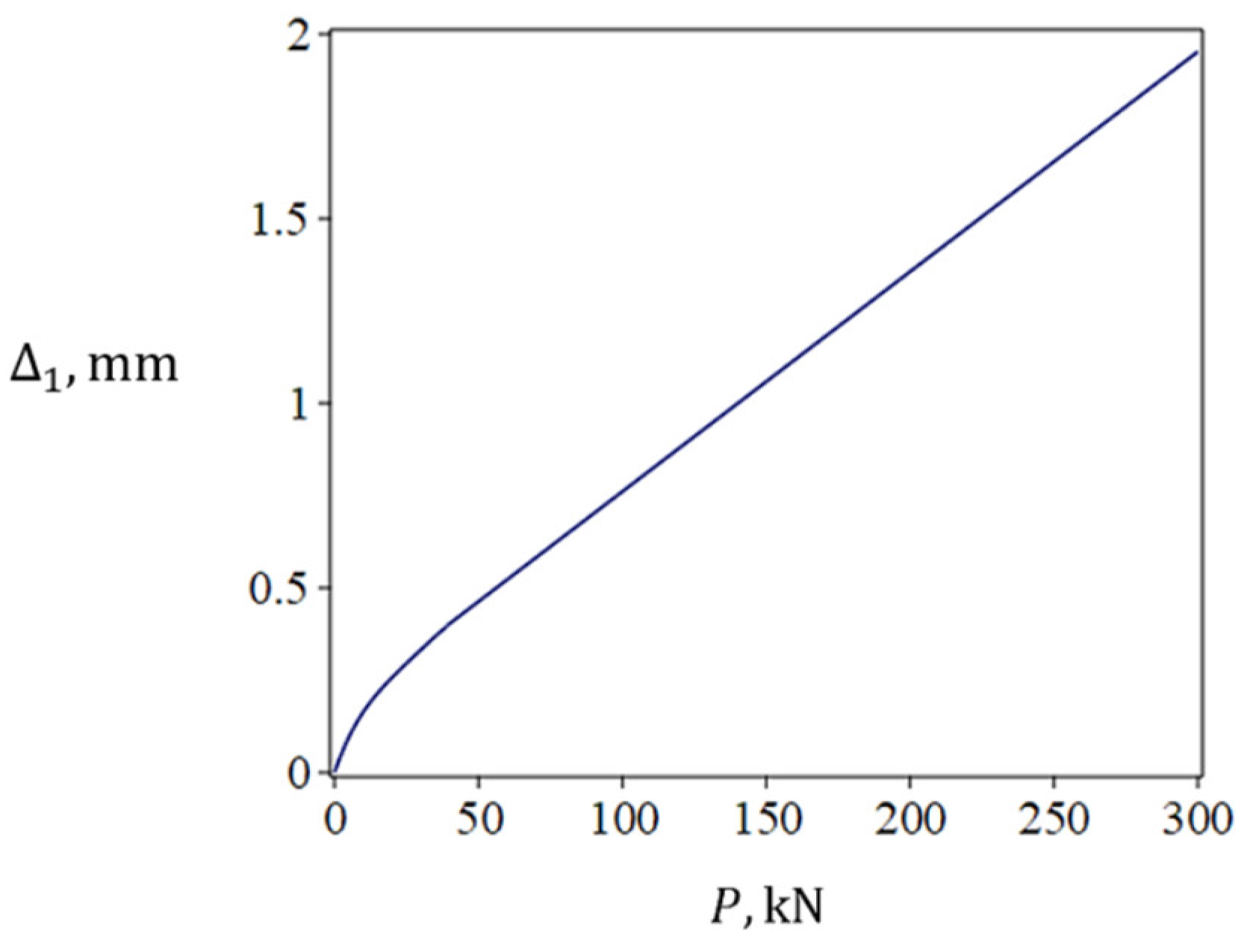
Respectively, in laboratory conditions, the correction value (17) is determined based on the test results of a virtual specimen with zero compliance ($C_2=0;$ in this case $K_2\to \infty$). This means that the force–displacement curve is plotted on an “empty” machine (without a specimen). In this case, the upper and lower plates directly interact across the contact surface with a force P.

If the displacement Δ₁ is linearly related to P, then the stiffness of the loading system is constant. However, in real conditions, the initial portion of the force–displacement curve is convex downward, because the stiffness of a real loading system increases with increasing load not instantly, but gradually over a short period.

Each additional link in the loading system increases its compliance and, accordingly, decreases its stiffness. This means that the actual compliance of the loading system must be determined before testing to determine the value of the correction factor (17).

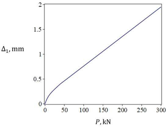
Figure 8 shows a plot of the correction (17) versus the compressive force for the testing machine used in this study (see Section 3.2). The curve is convex upward in the initial region because it is a displacement–load curve, i.e., an inverse load–displacement curve.

Figure 8. The experimental curve shows the correction values (17) to the measured displacements as a function of the measured force P. This curve is applicable only to the testing machine and its additional devices (if any) on which the curve was obtained. A similar curve must be obtained for each system consisting of the testing machine and its additional devices.

The equations for the practical determination of the corrections ${∆}_1$, obtained by approximating the experimental data of the above-mentioned virtual specimen with zero compliance ($C_2=0)$, have the following form:

$$\begin{array}{c}\mathrm{if} P\le 39\mathrm{kN}\mathrm{then}\hfill \\ {∆}_1=-0.1755972\times {10}^{-6}{P}^4+0.1937955\times {10}^{-4}{P}^3-0.8121482\times {10}^{-3}{P}^2+0.2274613\times {10}^{-1}P,R^2=0.9998;\hfill \\ \mathrm{i}\mathrm{f} P>39 \mathrm{k}\mathrm{N}\mathrm{then} {∆}_1=0.5959798\times {10}^{-2}P+0.1649199,R^2=0.9999.\hfill \end{array}$$

(18)

The displacement of a real specimen measured by a testing machine is denoted as Δ in Equations (10)–(15). Moving from theory to practice, we redesignate the measured displacement as ${∆}_{\mathrm{m}\mathrm{e}\mathrm{a}\mathrm{s}\mathrm{u}\mathrm{r}\mathrm{e}\mathrm{d}}$. The corrected displacement is denoted in Equations (12)–(15) as ${∆}_2$; for practical use, we redesignate the corrected displacement as ${∆}_{\mathrm{c}\mathrm{o}\mathrm{r}\mathrm{r}\mathrm{e}\mathrm{c}\mathrm{t}\mathrm{e}\mathrm{d}}$. Then, Equation (12) takes the following form (19):

$${{∆}_{\mathrm{c}\mathrm{o}\mathrm{r}\mathrm{r}\mathrm{e}\mathrm{c}\mathrm{t}\mathrm{e}\mathrm{d}} =∆}_{\mathrm{m}\mathrm{e}\mathrm{a}\mathrm{s}\mathrm{u}\mathrm{r}\mathrm{e}\mathrm{d}}-{∆}_1.$$

(19)

The force acting on the specimen $P=P_{\mathrm{m}\mathrm{e}\mathrm{a}\mathrm{s}\mathrm{u}\mathrm{r}\mathrm{e}\mathrm{d}}$ is always measured by the machine synchronously with the displacement ${∆}_{\mathrm{m}\mathrm{e}\mathrm{a}\mathrm{s}\mathrm{u}\mathrm{r}\mathrm{e}\mathrm{d}}$. This allows the value of ${∆}_1$ to be calculated using Equation (18).

The methodology considered was used in processing the results of rapakivi granite tests, presented in the following section.

3.2. Approximation of Test Results of Rapakivi Granite

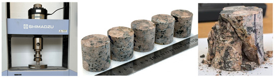
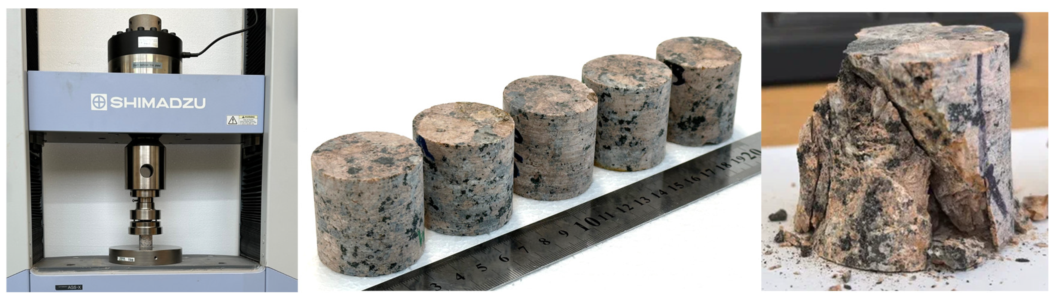
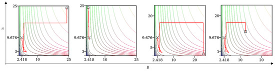
Based on the methodology presented in Section 2, we consider the pre-peak deformation stage of five cylindrical specimens of rapakivi granite from the Mustavara deposit (see Table 3 and Figure 9).

Table 3. Initial data and calculation results for rapakivi granite (Mustavara deposit, Karelia).

Specimen	$\mathit{n}$	$\mathit{B}$	${\mathit{\epsilon }}_{\mathit{c}}$	${\mathit{\sigma }}_{\mathit{c}}$(MPa)	${\mathit{\epsilon }}_{\mathit{E}}$	${\mathit{\epsilon }}_{\mathit{E}}/{\mathit{\epsilon }}_{\mathit{c}}$	${\mathit{\sigma }}_{\mathit{E}}$(MPa)	${\mathit{\sigma }}_{\mathit{E}}/{\mathit{\sigma }}_{\mathit{c}}$	$\mathit{E}$(GPa)	$\mathit{E}/{\mathit{\sigma }}_{\mathit{c}}$
1	9.68	2.42	0.0108	138.6	0.00859	0.794	99.1	0.715	24.9	179.6
2	6.86	2.39	0.00985	187.7	0.00735	0.746	126.2	0.672	35.5	189.1
3	8.00	2.90	0.00937	136.9	0.00741	0.791	94.43	0.689	31.2	227.9
4	4.96	2.82	0.00990	175.5	0.00717	0.724	111.15	0.633	34.9	198.8
5	4.48	2.84	0.00931	140.6	0.00661	0.710	87.35	0.621	29.5	209.5
Average	6.80	2.67	0.0098	155.9	0.00743	0.753	103.6	0.654	31.20	201.0
Standard deviation	1.92	0.22	0.00053	21.40	0.00065	0.034	13.7	0.028	3.87	16.7
Coefficient of variation, %	28	8.3	5.4	13.7	8.71	4.5	13.2	4.2	12.4	8.3

Figure 9. Test machine AGS-X 300 and specimens before and after testing.

The mineralogical composition of the specimens comprises the following: potassium feldspar—58%; plagioclase—7%; quartz—32%; biotite, hornblende, and ore minerals—the remaining 3%. Detailed mineralogical, geochemical, and geochronological aspects associated with rapakivi granites are discussed in [39,40].

All specimens have a diameter of 42.6 mm. The heights, listed in specimen numbering order (see Table 3), are 38.1, 39.0, 38.8, 38.5, and 39.8 mm, respectively.

Uniaxial compression tests were conducted on a test machine AGS-X 300 operated in displacement-control mode at a constant crosshead rate of 0.2 mm/min. The applied load was measured using an internal load cell (capacity 300 kN; accuracy ±1% full scale) and recorded at 100 Hz. Between 50,000 and 60,000 measurements were performed for each specimen. Displacement was determined using the method described in the previous section, using Formula (19).

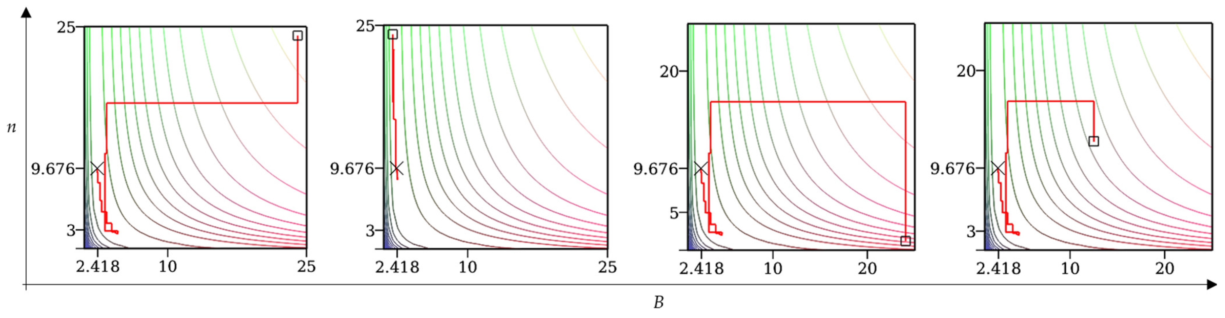
Figure 10 displays the search trajectories generated by the PROS algorithm [30] for the first specimen. The starting points are marked as squares, and the algorithm consistently converges to a single final point irrespective of the initial conditions.

Figure 10. Search trajectories of the PROS algorithm originating from various starting points, denoted by small squares. Regardless of the initial coordinates, the algorithm converges to the same final point with coordinates n = 9.676 and B = 2.418. A diagonal cross marks the final point.

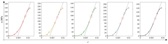
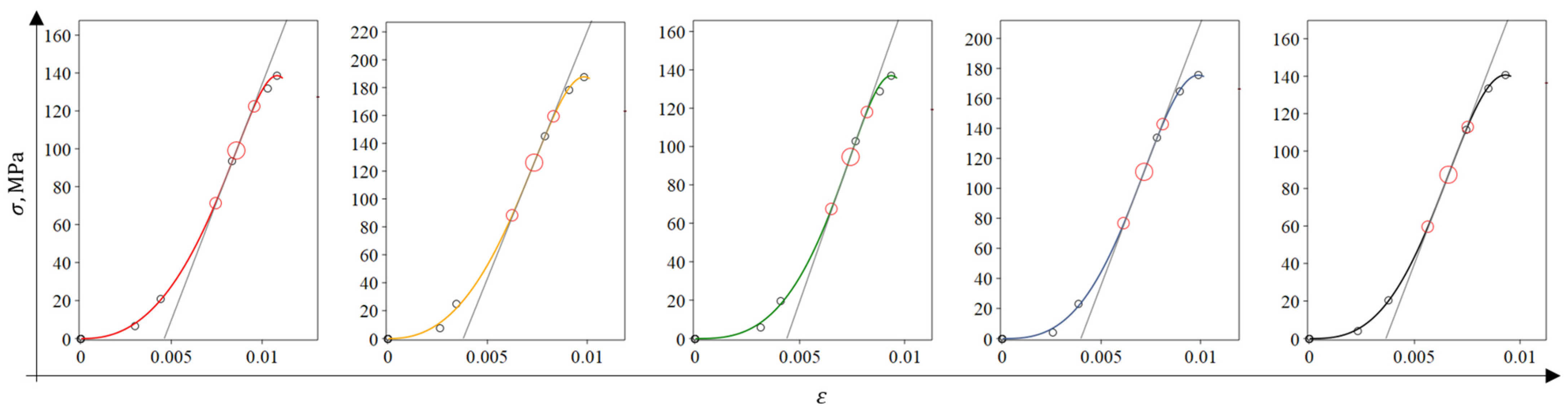
Using the determined values of parameters n and B, further calculations were performed according to the methodology described in Section 2 and based on Equation (2). This procedure resulted in the construction of stress–strain curves for five specimens (Figure 11).

Figure 11. Stress–strain curves constructed according to the methodology described in Section 2. Experimental data points are represented by black circles and were obtained using corrected measurements (19). The large red circle denotes the point at which the tangential modulus of elasticity $E={\displaystyle \frac{d\sigma }{d\epsilon }}$ reaches its maximum value; at this point, the second derivative of stress with respect to strain is zero: ${\displaystyle \frac{d^2\sigma }{d{\epsilon }^2}}=0$. Small red circles indicate the boundaries of the region that is visually perceived as a linear segment of the stress–strain curve. The gray inclined line represents the tangent drawn at the point where the mentioned second derivative is zero. The slope of this tangent line is numerically equal to the maximum value of the tangential modulus of elasticity.

It is important to note that the parameters n and B of Equation (2) have been determined for each specimen. This enables the analytical determination of not only the tangential modulus of elasticity at any point along the stress–strain curve—through differentiation of the equation—but also the energy-related characteristics of the deformation process. The latter can be obtained by integrating the proposed equation in subsequent studies, thereby facilitating a more comprehensive mechanical characterization.

Specifically, the tangential modulus of elasticity E at a given strain level ε can be derived as the first derivative of the stress function $\sigma \left(\epsilon \right)$ with respect to strain. Similarly, the specific strain energy (energy per unit volume) accumulated during deformation up to a certain strain ${\epsilon }^{*}$ can be calculated via integration ($W={\int }_0^{{\epsilon }^{*}}\sigma \left(\epsilon \right)d\epsilon$), which provides valuable insight into the material’s energy absorption capacity and failure mechanisms.

Additional experimental data obtained from uniaxial compression tests on rapakivi granite specimens are presented in Table 3. These results, illustrated in Figure 9, include key mechanical parameters and characteristic points of the stress–strain response, further supporting the validation and application of the proposed analytical approach.

In addition to the intrinsic geological characteristics, extrinsic experimental factors may also contribute to the observed differences. In particular, the rigidity (or stiffness) of the loading system used during mechanical testing can significantly affect the measured elastic modulus. Testing systems with lower rigidity may introduce compliance effects that artificially reduce the apparent stiffness of the specimen, thereby yielding lower tangent modulus values.

Consequently, to ensure robust and reliable interpretation of test results, it is recommended to employ multiple testing methods when characterizing rock mechanical properties, compare results obtained from different experimental setups, and continue systematic research to further elucidate the relationships between geological history, microstructure, and macroscopic mechanical response [41,42,43].

Furthermore, the approach discussed in this study demonstrates potential for application in approximating experimental data obtained under both static and dynamic loading conditions. This versatility enhances its utility in geotechnical engineering, where understanding material behavior across a range of strain rates and loading scenarios is essential for accurate modeling and design [44,45,46], including the adaptation and development of the considered approach to the analysis of the mechanical behavior of concrete as an artificial analysis of rock, taking into account new methodological approaches [47,48].

3.3. Scope and Limitations of the Proposed Data Approximation Approach

The scope of the applicability of the proposed approach to experimental data approximation is currently limited to testing granite and similar rock types. A related application domain includes testing of concrete specimens, as concrete serves as an artificial analog of natural rocks.

The implementation examples and supporting arguments presented in this article demonstrate the potential to mitigate the influence of subjective factors on the accuracy of displacement measurements and associated strain calculations during uniaxial compression testing of rock specimens. However, it should be emphasized that subjective influences in estimating the maximum tangential modulus of elasticity—using stress–strain curves—are not fully eliminated, but rather mitigated.

Certain subjectivity persists in the following aspects:

• Selection of the stress–strain curve function: In this study, an S-curve with two dimensionless parameters (n and B) is adopted;
• Criteria for identifying the linear region on the stress–strain curve, which is critical for accurate modulus calculation;
• Procedure for selecting intermediate data points (m ≥ 4), including their distribution across the strain range.

Further research is required to develop methods that can further mitigate these limitations. Such studies could focus on the following:

• Objective criteria for functional form selection;
• Automated algorithms for linear region identification;
• Optimization strategies for intermediate point selection, potentially leveraging machine learning or advanced statistical techniques, including sensitivity analysis to changes in parameter values.

4. Conclusions

To enhance the accuracy of approximating compression test results for granite and similar geomaterials compared to conventional methods, this study proposes an alternative procedure for fitting experimental data at the pre-peak stage. The proposed approach combines a modified S-curve equation with the purely random orthogonal search (PROS) optimization method [30].

Key findings and contributions of this work are summarized as follows:

Applied the PROS for parameter identification.

The study confirms the feasibility of applying the purely random orthogonal search (PROS), introduced in the literature in 2021, to determine the parameters of the approximating equation. This method enhances the objectivity and accuracy of experimental data analysis by reducing the influence of subjective factors within the defined experimental protocol.

Modified S-curve model with PROS-based parameter estimation.

A modified two-parameter S-curve equation is proposed for approximating experimental stress–strain data. The optimal values of the model parameters are determined by solving a two-dimensional objective function minimization problem using the PROS method. Notably, the dimensionality of the optimization problem remains independent of the number of experimental data points, which improves the computational efficiency.

Procedure for estimating the maximum tangential modulus of elasticity. A systematic procedure is developed and demonstrated for determining the maximum value of the tangential modulus of elasticity at the pre-peak stage of specimen deformation under uniaxial compression. The obtained results are in good agreement with the findings reported in existing studies, thereby validating the proposed approach.

Numerical correction of measured displacements in accordance with the virtual sensor concept. In the context of the challenges associated with accurate displacement measurement during uniaxial compression tests using soft testing machines, the concept of a virtual extensometer localized on the specimen is introduced. A numerical correction procedure is proposed and implemented to account for machine compliance and improve the reliability of the measured displacements.

Engineering implications. In the future, after further research, the proposed methodology for approximating experimental data using the PROS algorithm could be implemented in software for geotechnical testing machines.

Furthermore, to improve the accuracy of displacement determination during rock testing, the procedure for correcting measured displacements within the virtual extensometer concept, justified in this article, could be implemented in software for the same geotechnical testing machines. This correction procedure effectively functions as a virtual extensometer, providing displacement data comparable to that obtained from direct physical measurements on the specimen surface—without requiring additional hardware.

Future research directions. Potential extensions of the proposed computational framework include its adaptation for comparative geotechnical analysis of rocks from different geological deposits. Further development may also involve incorporating post-peak deformation behavior into the analysis, thereby enabling a more comprehensive characterization of rock mechanical responses across the entire stress–strain curve.

References

- Eberhardt, E.; Stead, D.; Stimpson, B.; Read, R.S. Identifying crack initiation and propagation thresholds in brittle rock. Can. Geotech. J. 1998, 35, 222–233. [Google Scholar] [CrossRef]
- Cai, M.; Kaiser, P.K.; Tasaka, Y.; Maejima, T.; Morioka, H.; Minami, M. Generalized crack initiation and crack damage stress thresholds of brittle rock masses near underground excavations. Int. J. Rock Mech. Min. Sci. 2004, 41, 833–847. [Google Scholar] [CrossRef] [Scilit]
- He, M.; Cheng, T.; Qiao, Y.; Li, H. A Review of Rockburst: Experiments, Theories, and Simulations. J. Rock Mech. Geotech. Eng. 2023, 15, 1312–1353. [Google Scholar] [CrossRef] [Scilit]
- Tang, L.; Wang, Y.; Sun, Y.; Chen, Y.; Zhao, Z. A Review on the failure modes of rock and soil mass under compression and the exploration about constitutive equations of rock and soil mass. Adv. Civ. Eng. 2022, 2022, 1–13. [Google Scholar] [CrossRef] [Scilit]
- Yang, B.; Song, C.; Duan, Y.; Zhao, Z. Relationship between crack initiation stress and uniaxial compressive strength of brittle rocks. Eng. Fract. Mech. 2025, 314, 110768. [Google Scholar] [CrossRef] [Scilit]
- Bieniawski, Z.T. Mechanism of brittle fracture of rock: Part II—Experimental studies. Int. J. Rock Mech. Min. Sci. Geomech. Abstr. 1967, 4, 407–423. [Google Scholar] [CrossRef] [Scilit]
- Eberhardt, E.; Stead, D.; Stimpson, B. Quantifying progressive pre-peak brittle fracture damage in rock during uniaxial compression. Int. J. Rock Mech. Min. Sci. 1999, 36, 361–380. [Google Scholar] [CrossRef] [Scilit]
- Liu, G.; Chen, Y.; Du, X.; Wang, S.; Fernández-Steeger, T.M. Evolutionary Analysis of Heterogeneous Granite Microcracks Based on Digital Image Processing in Grain-Block Model. Materials 2022, 15, 1941. [Google Scholar] [CrossRef] [Scilit]
- Zhao, X.G.; Cai, M.; Wang, J.; Li, P.F.; Ma, L.K. Objective determination of crack initiation stress of brittle rocks under compression using AE measurement. Rock Mech. Rock Eng. 2015, 48, 2473–2484. [Google Scholar] [CrossRef] [Scilit]
- Nicksiar, M.; Martin, C.D. Crack initiation stress in low porosity crystalline and sedimentary rocks. Eng. Geol. 2013, 154, 64–76. [Google Scholar] [CrossRef] [Scilit]
- Cai, M. Influence of intermediate principal stress on rock fracturing and strength near excavation boundaries—Insight from numerical modeling. Int. J. Rock Mech. Min. 2007, 45, 763–772. [Google Scholar] [CrossRef] [Scilit]
- Wu, J.; Li, C.; Hu, C. Relationship between crack initiation stress and uniaxial compressive strength of cemented waste rock-tailings backfill. Constr. Build. Mater. 2025, 499, 144097. [Google Scholar] [CrossRef] [Scilit]
- Dong, Q.; Li, C.; Liu, H.; Liu, Q.; Xu, Y. Research on Crack Propagation in Hard Rock Coal via Hydraulic Fracturing. Appl. Sci. 2025, 15, 11696. [Google Scholar] [CrossRef] [Scilit]
- Xu, H.; Putsikai, B.; Yu, S.; Yu, J.; Li, Y.; Gu, P. Numerical Simulation of Freezing-Induced Crack Propagation in Fractured Rock Masses Under Water–Ice Phase Change Using Discrete Element Method. Buildings 2025, 15, 2055. [Google Scholar] [CrossRef] [Scilit]
- Li, S.; Yang, H.; Li, Y.; Liu, X.; Tan, J.; Guo, Y.; Liang, Q.; Shen, Y.; Wei, X.; Ma, C. A Damage Constitutive Model for Rock Considering Crack Propagation Under Uniaxial Compression. Modelling 2025, 6, 116. [Google Scholar] [CrossRef] [Scilit]
- Lin, H.; Qiang, Y.; Li, L.; Li, H.; Liang, S. Investigating the closure stress and crack initiation stress in fractured rocks using the student t distribution and Monte Carlo simulation method. PLoS ONE 2024, 19, e0307804. [Google Scholar] [CrossRef] [Scilit]
- Qiang, Y.; Liu, G.; Xia, C.; Li, S.; Li, L.; Zhao, D.; Zhou, L.; Cheng, L. Study on closing and cracking stress calculation method of fractured rock. Front. Earth Sci. 2023, 10, 839304. [Google Scholar] [CrossRef] [Scilit]
- Chen, Z.; Liu, Z.; Chen, J.; Li, X.; Huang, L. Intelligent identification of acoustic emission Kaiser effect points and its application in efficiently acquiring in-situ stress. Int. J. Miner. Metall. Mater. 2025, 32, 1507–1518. [Google Scholar] [CrossRef] [Scilit]
- Bao, X.; Huang, S.; Lv, Y.; Huang, Y.; Wang, L.; Zhang, X. Study on Kaiser effect of granite under cyclic loading and unloading at different temperatures. Sci. Rep. 2025, 15, 11898. [Google Scholar] [CrossRef] [Scilit]
- Dai, J.; Liu, J.; Yang, J.; Ran, L.; Xue, F.; He, X. Correlational fractal analysis of the Kaiser effect in rock: Implications for salt-cavern engineering under triaxial cyclic loading and unloading. Nondestruct. Test. Eval. 2025, 40, 1180–1202. [Google Scholar] [CrossRef] [Scilit]
- Chang, J.; Manda, E.; Li, H.; Wang, Q.; Jing, Y. Rock crack initiation triggered by energy digestion. Sci. Rep. 2024, 14, 15222. [Google Scholar] [CrossRef] [Scilit] [PubMed]
- Briševac, Z.; Pollak, D.; Maričić, A.; Vlahek, A. Modulus of Elasticity for Grain-Supported Carbonates—Determination and Estimation for Preliminary Engineering Purposes. Appl. Sci. 2021, 11, 6148. [Google Scholar] [CrossRef] [Scilit]
- Selvarajan, S. A comprehensive study on modern optimization techniques for engineering applications. Artif. Intell. Rev. 2024, 57, 194–217. [Google Scholar] [CrossRef] [Scilit]
- Stojković, N.; Perić, D.; Stojić, D.; Marković, N. New stress-strain model for concrete at high temperatures. Teh. Vjesn. 2017, 24, 863–868. [Google Scholar] [CrossRef] [Scilit]
- Tang, Z.; Li, S.; Huang, S.; Huang, F.; Wan, F. Indirect estimation of rock uniaxial compressive strength from simple index tests: Review and improved least squares regression tree predictive model. Geotech. Geol. Eng. 2021, 39, 3843–3862. [Google Scholar] [CrossRef] [Scilit]
- Agoha, C.C.; Opara, A.I.; Bartholomew, D.C.; Osaki, L.J.; Agoha, U.K.; Njoku, J.O.; Akiang, F.B.; Epuerie, E.T.; Ibe, O.C. Application of artificial neural network and least squares regression technique in developing novel models for predicting rock parameters. Earth Sci. Inform. 2024, 17, 5671–5698. [Google Scholar] [CrossRef] [Scilit]
- Adorni, E.; Coïsson, E.; Ferretti, D. In situ characterization of archaeological adobe bricks. Constr. Build. Mater. 2013, 40, 1–9. [Google Scholar] [CrossRef] [Scilit]
- Amado, C.; Bianco, A.M.; Boente, G.; Rodrigues, I.M. Robust estimation of heteroscedastic regression models: A brief overview and new proposals. Stat. Pap. 2025, 66, 65. [Google Scholar] [CrossRef] [Scilit]
- Markou, G.; Bakas, N.; Papadrakakis, M.; Chatzichristofis, S. A General Framework of High-Performance Machine Learning Algorithms: Application in Structural Mechanics. Comput. Mech. 2024, 73, 705–729. [Google Scholar] [CrossRef] [Scilit]
- Plevris, V.; Bakas, N.P.; Solorzano, G. Pure Random Orthogonal Search (PROS): A Plain and Elegant Parameterless Algorithm for Global Optimization. Appl. Sci. 2021, 11, 5053. [Google Scholar] [CrossRef] [Scilit]
- Shekov, V.; Kolesnikov, G. Differential Energy Criterion for Brittle Fracture: Conceptualization and Application to the Analysis of Axial and Lateral Deformation in Uniaxial Compression of Rocks. Materials 2023, 16, 4875. [Google Scholar] [CrossRef] [Scilit]
- Blagojević, M.; Pešić, D.; Mijalković, M.; Glišović, S. Jedinstvena funkcija za opisivanje naprezanja i deformacije betona u požaru. Građevinar 2011, 63, 19–24. Available online: https://hrcak.srce.hr/clanak/96329 (accessed on 19 January 2026).
- Aboayanah, K.R.; Abdelaziz, A.; Haile, B.F.; Zhao, Q.; Grasselli, G. Evaluation of Damage Stress Thresholds and Mechanical Properties of Granite: New Insights from Digital Image Correlation and GB-FDEM. Rock Mech. Rock Eng. 2024, 57, 4679–4706. [Google Scholar] [CrossRef] [Scilit]
- Ma, Q.; Liu, X.; Tan, Y.; Wang, R.; Xie, W.; Wang, E.; Liu, X.; Shang, J. Experimental study of loading system stiffness effects on mechanical characteristics and kinetic energy calculation of coal specimens. Rock. Mech. Rock. Eng. Rock Mech. Rock. Eng. 2024 2024, 57, 9941–9957. [Google Scholar] [CrossRef] [Scilit]
- Yin, Y.; Zheng, W.; Tang, X.; Xing, M.; Zhang, Y.; Zhu, Y. Test study on failure and energy supply characteristics of rock under different loading stiffness. Eng. Fail. Anal. 2022, 142, 106796. [Google Scholar] [CrossRef] [Scilit]
- Hou, P.Y.; Cai, M. Post-peak stress-strain curves of brittle hard rocks under different loading environment system stiffness. Rock Mech. Rock Eng. 2023, 55, 3837–3857. [Google Scholar] [CrossRef] [Scilit]
- Abdelaziz, A.; Grasselli, G. How believable are published laboratory data? A deeper look into system-compliance and elastic modulus. J. Rock. Mech. Geotech. Eng. 2021, 13, 487–499. [Google Scholar] [CrossRef] [Scilit]
- Hudson, J.; Crouch, S.; Fairhurst, C. Soft, stiff and servo-controlled testing machines: A review with reference to rock failure. Eng. Geol. 1972, 6, 155–189. [Google Scholar] [CrossRef] [Scilit]
- Bulakh, A.G.; Popov, G.N.; Yanson, S.Y.; Ivanov, M.A. New data on the granite pedestal of the monument to Peter the Great “The Bronze Horseman” in Saint Petersburg. J. Min. Inst. 2021, 248, 180–189. [Google Scholar] [CrossRef] [Scilit]
- Abersteiner, A.; Rämö, O.T.; Kontonikas-Charos, A.; Kharkongor, M.; Karampelas, N.; Gilbert, S.E.; Wade, B.; Ambroziak-Murzyn, K.; Jarred, C.; Lloyd, J.C.; et al. Geochronological and geochemical insights into episyenite metasomatic overprint in the Proterozoic Suomenniemi rapakivi granite complex (Finland). Lithos 2025, 516–517, 108269. [Google Scholar] [CrossRef] [Scilit]
- Narimani, S.; Davarpanah, S.M.; Kovács, L.; Vásárhelyi, B. Variation of Elastic Stiffness Parameters of Granitic Rock during Loading in Uniaxial Compressive Test. Appl. Mech. 2023, 4, 445–459. [Google Scholar] [CrossRef] [Scilit]
- Tutluoğlu, L.; İbrahim, F.; Karpuz, C. Relationship between pre-failure and post-failure mechanical properties of rock material of different origin. Rock Mech. 2015, 48, 121–141. [Google Scholar] [CrossRef] [Scilit]
- Zhai, M.; Xu, C.; Xue, L.; Cui, Y.; Dong, J. Loading rate dependence of staged damage behaviors of granite under uniaxial compression: Insights from acoustic emission characteristics. Theor. Appl. Fract. Mech. 2022, 122, 103633. [Google Scholar] [CrossRef] [Scilit]
- Paul, S.; Chattopadhyaya, S.; Raina, A.K.; Sharma, S.; Li, C.; Zhang, Y.; Kumar, A.; Tag-Eldin, E. A Review on the Impact of High-Temperature Treatment on the Physico-Mechanical, Dynamic, and Thermal Properties of Granite. Sustainability 2022, 14, 14839. [Google Scholar] [CrossRef] [Scilit]
- Isaka, B.L.A.; Gamage, R.P.; Rathnaweera, T.D.; Perera, M.S.A.; Chandrasekharam, D.; Kumari, W.G.P. An Influence of Thermally-Induced Micro-Cracking under Cooling Treatments: Mechanical Characteristics of Australian Granite. Energies 2018, 11, 1338. [Google Scholar] [CrossRef] [Scilit]
- Jiang, Z.; Zhu, Z.; Accornero, F.; Lacidogna, G. Acoustic emission and digital image correlation evidence of size effects on the compression failure of concrete. Mag. Concr. Res. 2025, 77, 1060–1072. [Google Scholar] [CrossRef] [Scilit]
- Wang, W.; Li, Z.; Du, F.; Cao, Z.; Shi, J.; Zhai, M.; Liu, M. Study on the evolution law of failure depth of large mining height and ultra-wide working surface. Sci. Rep. 2026, 16, 665. [Google Scholar] [CrossRef] [Scilit]
- Lin, H.; Zhang, W.; Guo, S.; Zhang, X.; Wang, L.; Zhang, J. Study on the energy evolution mechanism and fractal characteristics of coal failure under dynamic loading. ACS Omega 2025, 10, 54710−54719. [Google Scholar] [CrossRef] [Scilit]
Disclaimer/Publisher’s Note: The statements, opinions and data contained in all publications are solely those of the individual author(s) and contributor(s) and not of MDPI and/or the editor(s). MDPI and/or the editor(s) disclaim responsibility for any injury to people or property resulting from any ideas, methods, instructions or products referred to in the content. |
© 2026 by the authors. Licensee MDPI, Basel, Switzerland. This article is an open access article distributed under the terms and conditions of the Creative Commons Attribution (CC BY) license.