A Comparison of Optimisation Algorithms for Electronic Polarisation Control in Quantum Key Distribution

Abstract

Polarisation encoding is widely used in fibre-based Quantum Key Distribution (QKD), but random birefringence in optical fibres causes the transmitted states to drift, requiring active compensation at the receiver. Electronic Polarisation Controllers (EPCs) are commonly used for this purpose, yet the relationship between their control voltages and the resulting polarisation transformation is highly nonlinear and difficult to model. While optimisation algorithms are frequently employed to align and stabilise polarisation states, their comparative performance has not been systematically studied in realistic QKD settings. In this work, we benchmark four optimisation algorithms for electronic polarisation control, using both a numerical model and a 50 km fibre-based experimental setup. We evaluate each algorithm in terms of convergence time, failure rate, and stability, under both initial alignment and continuous drift compensation scenarios. Coordinate Descent achieved the fastest average alignment time (2.1 ms in simulation; 34.6 s experimentally), while Simulated Annealing delivered perfect reliability. We further propose a hybrid control strategy that combines fast initial alignment with high-reliability realignment. This approach was validated over a continuous 2 h QKD simulation with real fibre drift, demonstrating robust polarisation control without manual intervention. Our results provide guidance for algorithm selection in practical QKD deployments and suggest a pathway to resilient, autonomous polarisation tracking in long-distance quantum networks.

1. Introduction

Quantum Key Distribution (QKD) [1,2,3] enables two parties to share encryption keys with unconditional security, leveraging fundamental principles of quantum mechanics such as measurement disturbance and the no-cloning theorem. A widely used implementation transmits single photons through standard single-mode fibre, where information is encoded in the polarisation state [4]. However, environmental perturbations such as temperature gradients, mechanical vibrations, or stress-induced birefringence cause random rotations of the polarisation states during transmission. These drifts rapidly degrade alignment between transmitter and receiver bases, increasing the Quantum Bit Error Rate (QBER) and ultimately lowering the QKD secret key rate.

To counteract these random drifts, the receiver must continually realign its measurement basis with the states prepared by the transmitter. This is commonly achieved using an Electronic Polarisation Controller (EPC) [5], which applies controlled birefringence through a set of piezoelectric fibre squeezers [6]. In principle, appropriate voltages on the EPC channels can implement any unitary polarisation transformation. In practice, however, the mapping from voltages to polarisation rotations is highly nonlinear, device-specific, and difficult to model analytically. As a result, EPCs are typically operated as black-box actuators whose control settings must be determined empirically.

Given the lack of an accurate analytical model for EPC behaviour, optimisation algorithms naturally lend themselves to the task of finding suitable control voltages. A variety of approaches have been demonstrated in the literature, including Gradient Descent methods for iterative polarisation alignment [7,8,9], Genetic Algorithms for global search over EPC settings [10], and stochastic techniques such as Simulated Annealing and Particle Swarm Optimisation [11]. Additional schemes based on heuristic search or adaptive control have also been proposed [12,13,14,15]. While each method has been shown to achieve polarisation alignment in specific contexts, a systematic comparison of their performance under realistic QKD conditions is still lacking.

Experimental characterisations of polarisation drift in deployed or laboratory fibre links show that alignment can require several minutes to recover after significant disturbances [16]. Such delays can markedly reduce the overall secret key rate, especially in systems where alignment interrupts quantum transmission. Therefore, identifying which optimisation strategies provide the fastest and most reliable convergence is essential for the development of autonomous, high-performance QKD systems. In this work, we perform both numerical simulations and a 50 km fibre-based experimental study to compare the behaviour of four optimisation algorithms in the context of initial alignment and continuous polarisation control.

The remainder of this paper is organised as follows. In Section 2, we describe the numerical model of the EPC and the experimental apparatus used for validation. Section 3 introduces the optimisation algorithms considered and the fitness function employed throughout. Simulation results, including hyperparameter tuning and algorithmic comparisons, are presented in Section 4, followed by experimental results in Section 5. Finally, Section 6 summarises our findings, discusses the physical origins of the observed behaviours, and outlines promising directions for future optimisation and modelling of EPC-based polarisation control.

2. Modelling in Simulation and Experimental Setup

In this section, we introduce the fitness function used by all optimisation algorithms, followed by the numerical models employed in simulation and the experimental apparatus used to validate the algorithms. Throughout this work, polarisation states are represented on the Poincaré sphere unless stated otherwise.

2.1. Fitness Function

All optimisation algorithms considered in this work require a quantitative measure of how close the current polarisation state is to the desired target state. We therefore define a fitness function f that returns the angular separation $\alpha$ between the current and target Stokes vectors on the Poincaré sphere. Minimising this angle corresponds directly to maximising the fidelity between the two states, making the alignment problem a natural minimisation task.

To compute this angular separation, we first express the polarisation states in Cartesian coordinates using their azimuth ($\phi$) and ellipticity ($\theta$) angles. These coordinates correspond directly to the normalised Stokes parameters:

$$\begin{array}{cc}\hfill S_1& =cos\theta cos\phi ,\hfill \\ \hfill S_2& =cos\theta sin\phi ,\hfill \\ \hfill S_3& =sin\theta .\hfill \end{array}$$

(1)

Given a current state $({\theta }_0,{\phi }_0)$ and a target state $({\theta }_T,{\phi }_T)$, their associated Stokes vectors are as follows:

$$\begin{array}{cc}\hfill {\overrightarrow{S}}_0& =(cos{\theta }_{0}cos{\phi }_0,cos{\theta }_{0}sin{\phi }_0,sin{\theta }_0),\hfill \\ \hfill {\overrightarrow{S}}_T& =(cos{\theta }_{T}cos{\phi }_T,cos{\theta }_{T}sin{\phi }_T,sin{\theta }_T),\hfill \end{array}$$

(2)

where both vectors have unit norm. The angular distance $\alpha$ between the two vectors is given by the following:

$${\overrightarrow{S}}_0·{\overrightarrow{S}}_T=cos\alpha .$$

(3)

Thus the fitness function is defined as

$$f({\overrightarrow{S}}_0,{\overrightarrow{S}}_T)=\alpha ={cos}^{-1}({\overrightarrow{S}}_0·{\overrightarrow{S}}_T),$$

(4)

which provides a smooth and interpretable error metric on the Poincaré sphere.

The angular error $\alpha$ in Equation (4) directly quantifies the distinguishability between the current and target polarisation states. Interpreting the normalised Stokes vectors as qubit states on the Bloch sphere, the fidelity between the two pure states is given by $F={cos}^2(\alpha /2)$, and the corresponding QBER is simply the infidelity:

$$\mathrm{QBER}=1-F={sin}^2\left({\displaystyle \frac{\alpha }{2}}\right).$$

(5)

This relation captures the intuitive fact that larger angular deviations on the Poincaré sphere translate directly into higher error rates in a polarisation-encoded QKD protocol. To illustrate this connection, consider an imperfect state prepared by Alice as

$$|\psi ⟩=cos\left({\displaystyle \frac{\alpha }{2}}\right)|H⟩+sin\left({\displaystyle \frac{\alpha }{2}}\right)|V⟩,$$

and assume Bob performs an ideal measurement in the $\left\{\right|H⟩,|V⟩\}$ basis. The probability of an erroneous measurement outcome is then exactly Equation (5). Consequently, minimising the angular error $\alpha$ is equivalent to minimising QBER arising from polarisation misalignment.

Throughout both simulation and experiment, we define successful convergence as achieving a fitness value of $\alpha \le 0.01$ rad, corresponding to a QBER of $2.5\times {10}^{-5}$. For comparison, the EPC datasheet (OZ Optics, Carp, ON, Canada, EPC-400) specifies a polarisation tolerance of ≈$4.636\times {10}^{-3}$ radians, which corresponds to a QBER of $4.8\times {10}^{-6}$. In the BB84 protocol [1], the security threshold $\mathrm{QBER}<11\%$ [17] corresponds to an angular deviation of approximately $0.67$ rad.

2.2. Simulation

Numerical simulations were conducted to study the behaviour of the optimisation algorithms under controlled and repeatable conditions before implementing them experimentally. The simulations provide qualitative insight into convergence speed, stability, and failure rates, though quantitative agreement with experiment is not expected due to simplifications in the device and channel models.

The simulation framework developed in [18] models three key components of the system: the optical channel, the EPC, and a polarimeter. These models capture the essential behaviour needed for comparing optimisation strategies while allowing large-scale statistical tests to be performed efficiently.

2.2.1. Channel Model

The simulated channel applies a random, time-varying birefringence to the transmitted polarisation state. Given an input state specified by ellipticity and azimuth $(\theta ,\phi )$, the state can be represented as the Stokes parameters $S_1$, $S_2$, and $S_3$ as given in Equation (1).

A new point on the Poincaré sphere can now be generated according to the scheme given by Muller [19]:

$$\overrightarrow{S^{\prime }}=(N(S_1,d),N(S_2,d),N(S_3,d))$$

(6)

where d is a tunable drift factor setting the effective step size. From here on, as the ellipticity and azimuth angles are the only parameters of interest for this new point, there is no requirement to re-normalise $\overrightarrow{S^{\prime }}$. The ellipticity and azimuth angles of this new point can then be obtained by the following:

$$\begin{array}{cc}\hfill {\theta }^{\prime }& ={\displaystyle \frac{1}{2}}\mathrm{atan}2\left(S_3^{\prime },\sqrt{S_1^{\prime 2}+S_2^{\prime 2}}\right)\hfill \\ \hfill {\phi }^{\prime }& ={\displaystyle \frac{1}{2}}\mathrm{atan}2(S_2^{\prime },S_1^{\prime })\hfill \end{array}$$

(7)

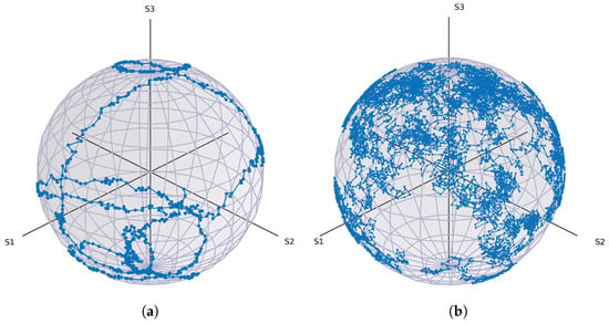
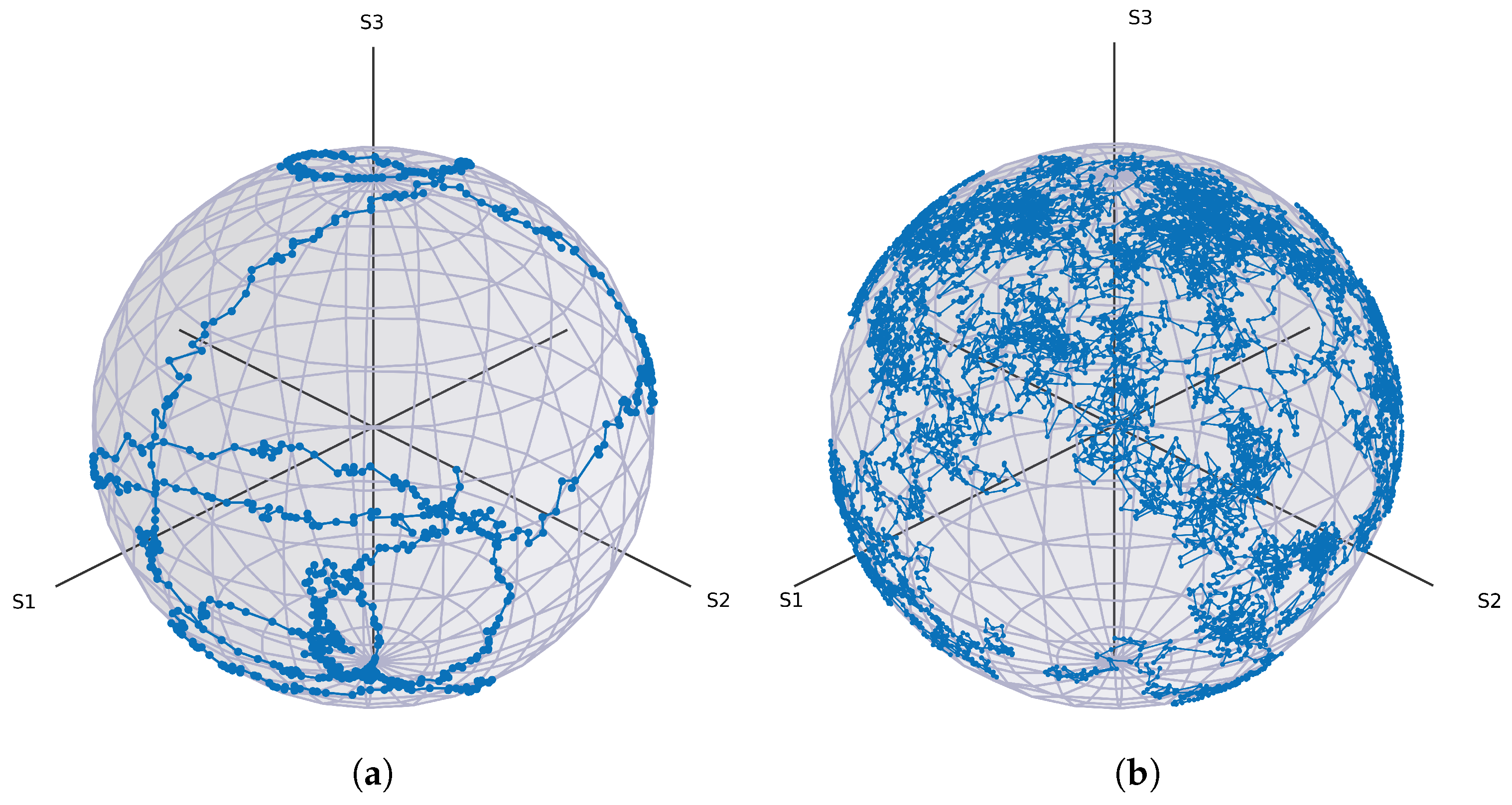
This produces small, continuous fluctuations in the polarisation state, as shown in Figure 1b. Figure 1a shows the corresponding drift measured experimentally over a 50 km fibre spool. While small-scale fluctuations resemble Brownian motion, the experimental trace also exhibits slower, larger-scale drifts not captured by the simple random-walk model.

Figure 1. (a) Measured polarisation drift over a 50 km single-mode fibre spool. Data points are subsampled for clarity, showing the first 25 min of a 2-h trace. (b) Simulated polarisation drift generated using the random-walk channel model described in Section 2. The experimental trace exhibits both fast fluctuations and slower drifts, whereas the simulation captures only the short-timescale stochastic component.

2.2.2. EPC Model

The EPC is modelled as a sequence of four ideal waveplate rotations acting on the input Stokes vector. In accordance with the theoretical structure of in-fibre piezoelectric controllers, the four channels implement rotations of the form

$$R_X\left({\theta }_1\right),R_Z\left({\theta }_2\right),R_X\left({\theta }_3\right),R_Z\left({\theta }_4\right),$$

where the control parameters ${\theta }_i$ are proportional to the integer-valued voltages applied to the simulated EPC channels. Each voltage $x\in [-5000,5000]$ is mapped to a rotation angle via

$$\theta \left(x\right)={\displaystyle \frac{x}{5000}}\times 2\pi ,$$

(8)

corresponding to a full $2\pi$ retardance across the controller’s voltage range. This idealised model reflects the theoretical capability of a four-waveplate sequence to implement any unitary polarisation transformation, but it does not capture non-ideal effects such as axis misalignment, nonlinear voltage–retardance responses, or coupling between channels observed in practical EPCs.

2.2.3. Polarimeter Model

The simulated polarimeter performs a measurement of the polarisation state, returning the corresponding azimuth and ellipticity angles. This ideal measurement model is sufficient for algorithmic benchmarking but does not include instrumental noise, calibration offsets, or wavelength-dependent sensitivity that may arise in real devices.

2.3. Experimental Setup

To validate the simulation results and assess the behaviour of the optimisation algorithms under realistic conditions, we implemented a fibre-based experimental setup. Two types of experiments were performed: (i) polarisation state generation, in which the algorithm drives the EPC to create a specified target state from an arbitrary input; (ii) continuous polarisation control, in which the algorithm must maintain a fixed target state in the presence of time-varying drift introduced by a long fibre spool. These complementary tests characterise both the static and dynamic performance of each optimisation method, providing insight into their suitability for practical QKD systems.

2.3.1. Operation Principle

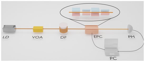
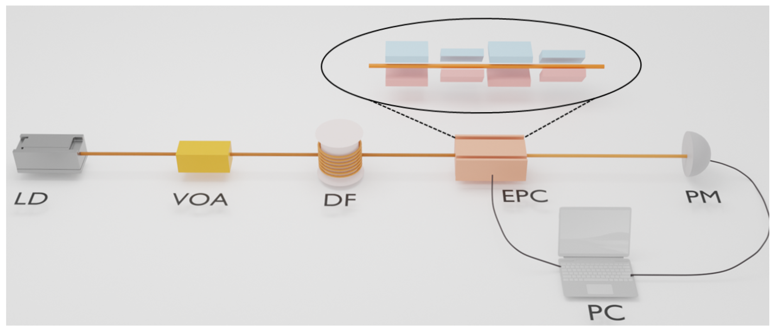
In the experimental setup shown in Figure 2, an in-fibre EPC is used to manipulate the polarisation state of light by inducing controlled birefringence. EPCs exploit the fact that mechanical stress modifies the refractive indices experienced by orthogonal polarisation components [20]. By squeezing, bending, or twisting the fibre, the device introduces a phase retardance between the fast and slow axes, thereby rotating the output polarisation state on the Poincaré sphere.

Figure 2. Experimental setup for state-generation and continuous polarisation-control tests. LD: laser diode; VOA: variable optical attenuator; DF: 50 km fibre spool; EPC: electronic polarisation controller; PM: polarimeter; PC: feedback computer. The EPC consists of four piezoelectric fibre squeezers rotated by ${\displaystyle \frac{\pi }{4}}$ relative to one another, enabling arbitrary polarisation transformations. The polarimeter provides real-time measurements that are used by the optimisation algorithm to update the EPC voltages.

The EPC used in our experiments is the OZ Optics EPC-400 [21], which consists of four piezoelectric fibre squeezers arranged sequentially, each rotated by ${\displaystyle \frac{\pi }{4}}$ with respect to the previous stage. Applying a voltage in the range $[-5000,5000]\mathrm{mV}$ produces a mechanical force of up to $25\mathrm{N}$ on the fibre, resulting in a tunable retardance $\mathsf{\Gamma }$ [22]. This behaviour can be modelled using a series of waveplates: two quarter-wave ($\lambda /4$) plates and two half-wave ($\lambda /2$) plates, alternated and oriented at fixed angles. Quarter-wave plates introduce a retardance of $\mathsf{\Gamma }=\pi /2$ and half-wave plates $\mathsf{\Gamma }=\pi$, where

$$\mathsf{\Gamma }={\displaystyle \frac{2\pi }{\lambda }}\Delta nL,$$

with $\lambda$ the wavelength, $\Delta n$ the induced birefringence, and L the effective interaction length [23]. The overall transformation implemented by the EPC is therefore well described by a sequence of Jones matrices with ${\mathbf{E}}_{in}$ representing the electric field components of the light entering the EPC and ${\mathbf{E}}_{out}$ representing the transformed electric field components exiting the EPC:

$${\mathbf{E}}_{out}=\mathbf{J}({\mathsf{\Gamma }}_4,\pi /4)\mathbf{J}({\mathsf{\Gamma }}_3,0)\mathbf{J}({\mathsf{\Gamma }}_2,\pi /4)\mathbf{J}({\mathsf{\Gamma }}_1,0){\mathbf{E}}_{in},$$

(9)

where each

$$\mathbf{J}({\mathsf{\Gamma }}_i,{\alpha }_i)=\left(\begin{array}{cc}cos({\mathsf{\Gamma }}_i/2)+isin({\mathsf{\Gamma }}_i/2)cos\left(2{\alpha }_i\right)& isin({\mathsf{\Gamma }}_i/2)sin\left(2{\alpha }_i\right)\\ isin({\mathsf{\Gamma }}_i/2)sin\left(2{\alpha }_i\right)& cos({\mathsf{\Gamma }}_i/2)-isin({\mathsf{\Gamma }}_i/2)cos\left(2{\alpha }_i\right)\end{array}\right)$$

(10)

denotes a waveplate with retardance ${\mathsf{\Gamma }}_i$ and fast-axis orientation ${\alpha }_i$ [24]. This configuration is sufficient to realise any rotation on the Poincaré sphere, and therefore any unitary transformation on a polarisation qubit.

2.3.2. Experimental Apparatus

A continuous-wave (CW) laser at $1550\mathrm{nm}$ (Thorlabs, Newton, NJ, USA, SFL1550P, 40 mW) [25] serves as the optical source. The output is attenuated using a variable optical attenuator (VOA) to approximately $40\mathsf{\mu }\mathrm{W}$ to prevent saturation of the polarimeter. Depending on the experiment, the light is then routed through either a short delay fibre or a $50\mathrm{km}$ ultra-low-loss single-mode fibre spool, which introduces slow, stochastic polarisation drift representative of real-world deployment conditions. Two experimental configurations were implemented:

• State generation. In this configuration, the EPC is placed after a $1\mathrm{m}$ section of single-mode fibre, and the polarimeter is positioned directly after the EPC to act as a real-time feedback device. The short fibre length ensures that the input polarisation state remains effectively constant throughout each run; therefore, each trial begins by applying a random initial voltage vector to the EPC, generating an arbitrary starting polarisation state. The optimisation algorithm must then drive the system to the specified target state as quickly and reliably as possible.
• Continuous control. To evaluate the ability of each algorithm to maintain alignment under realistic channel drift, a $50\mathrm{km}$ fibre spool is inserted between the VOA and the polarimeter. Over this distance, temperature fluctuations and mechanical relaxation induce continuous, slow-varying polarisation changes, providing a natural testbed for long-term stabilisation. The optimisation algorithm receives polarimeter feedback at each iteration and must compensate for the drift in real time to hold the output state near the target.

Together, these two configurations capture both the static and dynamic aspects of EPC control, enabling a comprehensive comparison of optimisation strategies for QKD applications.

3. Algorithm Specification

In this section, we describe the optimisation algorithms evaluated in this work: Gradient Descent, an adaptive step-size variant of Gradient Descent, Coordinate Descent, Simulated Annealing, and Genetic Algorithms. These methods were selected because they are widely used in practice for EPC-driven polarisation alignment, are conceptually simple, and require minimal computational overhead, an important consideration for real-time QKD operation.

A variety of other optimisation strategies have been proposed for polarisation control, including Golden Section Search [26], the Nelder–Mead simplex method [27], and other heuristic or derivative-free schemes [13,14]. While these approaches can perform well in specific scenarios, they tend to be more complex to implement. For this initial comparative study, we therefore restrict attention to five well-established algorithms that span both local and global optimisation paradigms.

Among the algorithms considered, Genetic Algorithms were ultimately excluded from the continuous-control experiments due to their significantly higher computational cost and slower convergence relative to the other methods. The practical limitations of applying population-based optimisers in an online polarisation-tracking context are discussed later in this section.

For each of the remaining algorithms—Gradient Descent, Adaptive Gradient Descent, Coordinate Descent, and Simulated Annealing—the pseudocode is provided in Appendix A. Below we summarise the operating principles of each method and describe how the fitness function defined in Section 2.1 is incorporated into their update rules.

In what follows, we denote by f the fitness function defined in Section 2.1, which returns the angular error $\alpha$ between the current and target polarisation states on the Poincaré sphere. The control variables of all optimisation algorithms are the EPC voltages, collected into a vector

$$\overrightarrow{v}=(v_1,v_2,v_3,v_4),$$

where each component $v_i$ corresponds to the drive voltage applied to one EPC channel. For a given voltage vector $\overrightarrow{v}$, we write $f\left(\overrightarrow{v}\right)$ for the fitness value obtained by measuring the resulting polarisation state with the polarimeter.

• Fixed Step-Size Gradient Descent

In the fixed step-size variant of Gradient Descent, one of the voltages $v_i\in \overrightarrow{v}$ is updated according to

$$v_i\leftarrow v_i-s,$$

(11)

where the voltage to modify is determined according to

$$i^{*}={\mathrm{argmin}}_{v_i\in \overrightarrow{v}}{\displaystyle \frac{\partial f}{\partial v_i}}.$$

(12)

The partial derivative is approximated numerically by finite differences. The step size s remains constant throughout the optimisation process.

A fixed step size offers conceptual and implementation simplicity, and it performs well when the fitness landscape is smooth and the algorithm is already reasonably close to the target state. However, selecting an appropriate value of s is critical: a value that is too small leads to slow convergence, whereas a value that is too large causes overshooting, oscillations, or divergence. Because the voltage–polarisation response of practical EPCs is highly nonlinear, the optimal step size is often device- and state-dependent, which motivates exploring adaptive variants of Gradient Descent.

• Adaptive Step-Size Gradient Descent

The limitations of fixed step-size Gradient Descent can be mitigated by allowing the step size to vary during the optimisation process. Intuitively, when the angular error is large, larger steps accelerate convergence, while closer to the target state, smaller steps improve stability and reduce overshooting.

To capture this behaviour, we employ a fitness-dependent step-size schedule of the form

$$s\left(f\right)=k\sqrt{f\left(\overrightarrow{v}\right)},$$

(13)

where k is a tunable constant. This schedule ensures that the step-size decreases smoothly as the algorithm approaches the target state, reflecting the need for finer adjustments at small angular errors.

The update rule for Adaptive Gradient Descent mirrors that of Gradient Descent,

$$v_i\leftarrow v_i-s\left(f\right),$$

(14)

with the distinction that the step-size $s\left(f\right)$ is recalculated at every iteration. This adaptive mechanism reduces oscillatory behaviour and improves convergence reliability, particularly in regions where the EPC’s voltage–polarisation response exhibits higher sensitivity.

Similar to fixed step-size Gradient Descent, Adaptive Gradient Descent identifies the best voltage input to optimise as specified in Equation (12) at each iteration of the algorithm. This process involves a significant number of operations, which introduces a significant increase in execution time, which the Coordinate Descent algorithm looks to circumvent.

For the remainder of this work, we refer to the fixed step-size method simply as Gradient Descent, and the fitness-dependent method as Adaptive Gradient Descent. We treat them as distinct optimisation algorithms in the comparisons that follow.

• Coordinate Descent

Coordinate Descent (CD) is an optimisation method that optimises one control variable at a time rather than optimising within the full multidimensional space [28]. In the context of EPC control, this means adjusting a single voltage component $v_i$ while keeping the remaining components fixed.

CD evaluates the fitness of the two neighbouring points of the variable $v_i$ to be optimised to determine which direction to optimise in, or if the variable is already at a minimum. If the variable $v_i$ is not at a minimum, it is optimised with a fixed step-size s using the same update scheme specified by Equation (11) repeatedly until the fitness value reaches a minimum. This foregoes the expensive process of checking which channel is optimal to update at each iteration, as with Gradient Descent and Adaptive Gradient Descent.

Various methods for selecting the control variable $v_i$ to optimise include: (i) a fixed cyclic order, (ii) random selection, or (iii) performing the control variable testing described in Equation (12) to find the locally optimal variable to optimise. In this work, we adopt the third strategy: selecting the coordinate axis and direction associated with the largest fitness decrease. While this choice generally improves convergence, it requires additional fitness evaluations per iteration.

A key advantage of Coordinate Descent is that it avoids estimating gradients in the full four-dimensional voltage space, making it computationally lightweight, and reduces the number of expensive operations involving optical components, theoretically greatly reducing the execution time.

However, like Gradient Descent, Coordinate Descent may become trapped in local minima above the acceptance threshold. Because the method restricts movement to coordinate-aligned directions, it may also require more iterations when the fitness landscape contains narrow valleys not aligned with the coordinate axes. Nevertheless, as shown in our results, CD exhibits strong practical performance and achieves the fastest average convergence amongst the algorithms tested.

• Simulated Annealing

Simulated Annealing (SA) [29] is a global optimisation method inspired by thermodynamic annealing processes, in which a material is slowly cooled so that it settles into a low-energy crystalline state. In the optimisation context, the “energy” corresponds to the fitness value, and the algorithm seeks the global minimum by probabilistically accepting non-improving moves.

At each iteration, SA generates a random neighbouring candidate solution ${\overrightarrow{v}}^{\prime }$ by perturbing the current voltage vector $\overrightarrow{v}$. The fitness values $f\left(\overrightarrow{v}\right)$ and $f\left({\overrightarrow{v}}^{\prime }\right)$ are then compared. If the candidate improves the fitness, i.e., $f\left({\overrightarrow{v}}^{\prime }\right)<f\left(\overrightarrow{v}\right)$, it is accepted unconditionally. Otherwise, the candidate is accepted with probability

$$P_{\mathrm{accept}}=exp\left(-{\displaystyle \frac{f\left({\overrightarrow{v}}^{\prime }\right)-f\left(\overrightarrow{v}\right)}{T}}\right),$$

(15)

where T is the current temperature parameter. This acceptance rule, known as the Metropolis criterion [30], enables the algorithm to escape local minima by occasionally accepting worse solutions, particularly when the temperature is high.

After each iteration, the temperature is decreased according to a cooling schedule, typically of the form

$$T\leftarrow \alpha T,$$

with $0<\alpha <1$. As the temperature decreases, the probability of accepting worse solutions declines, and the algorithm gradually transitions from global exploration to local refinement.

The strength of Simulated Annealing lies in its ability to escape local optima, an essential feature given the highly non-convex relationship between EPC voltages and the resulting polarisation transformation. As demonstrated in our experimental results, SA exhibits exceptional reliability, achieving a 0% failure rate under both simulation and laboratory conditions.

However, Simulated Annealing also has limitations. If the temperature decreases too quickly, the algorithm may “freeze” before reaching a solution below the acceptance threshold. Conversely, if the cooling schedule is too slow, convergence becomes excessively time-consuming. Successful deployment, therefore, requires careful selection of the initial temperature, neighbourhood generation mechanism, and cooling schedule.

• Genetic Algorithms

Genetic Algorithms (GAs) [31] are population-based meta-heuristic algorithms inspired by natural selection. A GA maintains a population of candidate solutions (individuals) modelled by chromosomes, evaluates their fitness, and iteratively generates new populations through selection, crossover, and mutation. Over successive generations, the population is expected to evolve toward regions of high fitness.

In each generation, individuals are selected, with probability biased toward fitter candidates, to serve as parents. New individuals are produced through crossover operations that recombine parent chromosomes, while random mutations introduce diversity. The process continues until either convergence is achieved or a predefined number of generations is reached.

Although GAs are powerful global optimisers and have been successfully applied to polarisation alignment in prior work, they are not well suited to the real-time constraints of EPC control in QKD systems. The primary limitation arises from the large number of fitness function evaluations required: even simple benchmark problems typically require populations exceeding 100 individuals and at least 10 generations to converge [32], yielding on the order of ${10}^3$ fitness evaluations. More complex optimisation tasks may require population sizes of several hundreds, and dozens of generations, with total evaluations exceeding ${10}^4$.

In our context, each fitness evaluation corresponds to a full EPC update and polarimeter measurement, making these evaluations time-consuming and resource-intensive. For comparison, fixed step-size Gradient Descent requires, on average, only 566 fitness evaluations, two orders of magnitude fewer than a typical GA. This discrepancy makes GAs impractical for the rapid and continuous control required in QKD deployments. For these reasons, we exclude Genetic Algorithms from the experimental and continuous-control studies that follow, focusing instead on optimisation methods that achieve comparable performance with significantly lower overhead.

Having introduced the optimisation algorithms and their operational principles, we now evaluate their performance under numerical simulations that model both the EPC behaviour and realistic polarisation drift.

4. Simulated Results

Before running the simulations, we formulated qualitative hypotheses about the relative performance of the four optimisation algorithms.

First, we hypothesised that Adaptive Gradient Descent would achieve both a shorter average optimisation time and a lower failure rate than fixed step-size Gradient Descent. The intuition is that adapting the step size as a function of the fitness mitigates the main drawback of standard GD: a single, globally chosen step size that is either too small (leading to slow convergence) or too large (hindering refinement). By design, Adaptive GD should approach the target state quickly with large initial steps and then refine with smaller steps, thereby reducing both the time to convergence and the probability of becoming trapped in local minima.

Second, we expected Coordinate Descent to further reduce the average optimisation time compared to Adaptive Gradient Descent. Because CD updates one EPC channel at a time, and in our implementation selects the coordinate and direction that yield the steepest local improvement, the number of fitness evaluations required to locate a good update is reduced. However, we did not have a clear prior expectation for how this strategy would affect the failure rate, since restricting motion to coordinate-aligned directions may make some local minima harder to escape.

Finally, we hypothesised that Simulated Annealing would have the lowest failure rate among all algorithms, but a longer average optimisation time. SA explores the search space globally by occasionally accepting worse solutions at high temperature, which should help it escape local optima. However, this global exploration comes at the cost of requiring many iterations before the temperature is low enough to permit fine-grained refinement. As a result, we anticipated that SA would be slower than Coordinate Descent and possibly slower than both variants of Gradient Descent.

Before making a final comparison across algorithms, several hyperparameters must be chosen for the specific task of initial polarisation alignment. Gradient Descent and Coordinate Descent each require a fixed step size; Simulated Annealing requires an initial temperature and cooling coefficient; Adaptive Gradient Descent requires a functional relationship between fitness and step size. In the following subsections, we describe how these parameters were selected and analyse the resulting trade-offs between average optimisation time and failure rate.

4.1. Gradient Descent

The first algorithm we consider is fixed-step-size Gradient Descent (GD). At each iteration, one of the four EPC control voltages is perturbed by a constant amount, and the algorithm selects the perturbation that yields the largest reduction in the fitness value. Because the optimal step size is not known a priori, we performed a parameter sweep to identify an appropriate operating point for the initial alignment task.

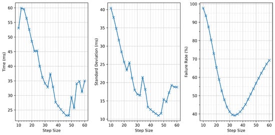
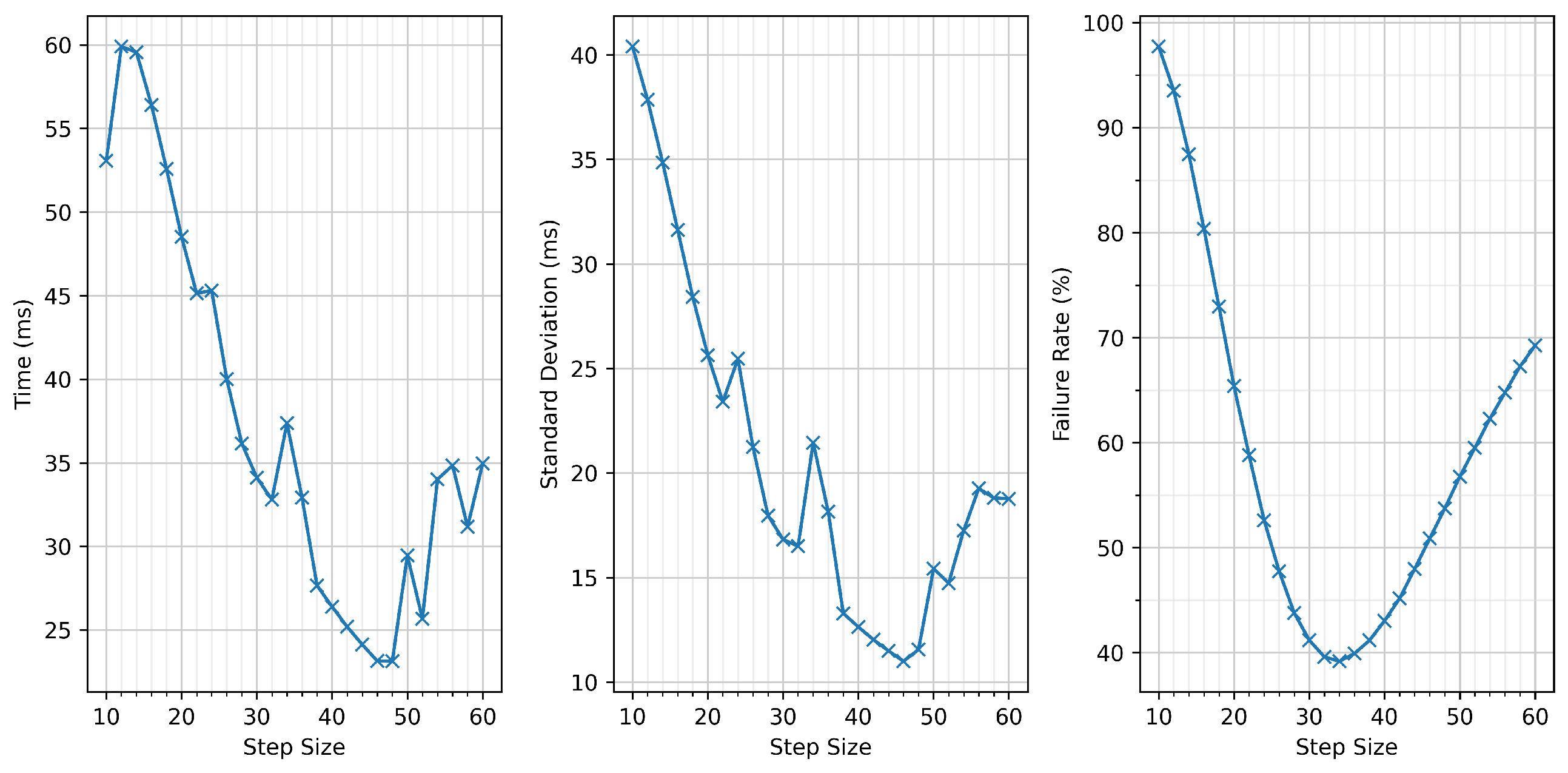
We evaluated 26 step sizes in the range 10–60 (inclusive) with increments of 2. For each step size, we performed 500,000 independent simulations of initial polarisation alignment and recorded the average optimisation time, the corresponding standard deviation, and the failure rate. The results are shown in Figure 3.

Figure 3. Performance of Gradient Descent for step sizes between 10 and 60 (in increments of 2), evaluated over 500,000 simulated initial-alignment trials per point. (left): average optimisation time; (centre): standard deviation; (right): failure rate. A step size of 40 minimises the failure rate while offering competitive optimisation time.

Two clear behaviours emerge. First, the average optimisation time decreases as the step size increases. Larger steps allow the algorithm to traverse the fitness landscape more rapidly, reaching the vicinity of the target state in fewer iterations. Second, the failure rate exhibits a well-defined minimum at a step size of 34. For step sizes smaller than 34, GD is more likely to stall near saddle points or shallow local minima, lacking the ability to “jump over” these regions. For step sizes larger than 34, the algorithm reaches the target region quickly but is unable to refine the solution with sufficient precision, resulting in premature termination above the acceptance threshold.

For the comparative evaluation of algorithms presented later, we selected a step size of 40, which provides a low failure rate, whilst also providing a competitive average optimisation time. This gave an average optimisation time of $26.392\mathrm{ms}$, with a standard deviation of $12.641\mathrm{ms}$ and a failure rate of $43.029\%$ (all rounded to three decimal places). Although slightly larger step sizes yield faster average convergence, the accompanying increase in failure rate was deemed too substantial to justify their use.

4.2. Adaptive Gradient Descent

For Adaptive Gradient Descent, the central design choice is how the step size should vary as a function of the current fitness value. Fixed step-size GD suffers from an inherent trade-off: a small step size enables precise refinement but slows global progress, whereas a large step size accelerates coarse alignment but prevents convergence to the required tolerance. An adaptive schedule seeks to balance these opposing requirements by using large steps when the angular error is high and progressively smaller steps as the algorithm approaches the target state.

We initially considered a linear dependency of the form $S\propto f$, where S is the step size and f the current fitness value. However, early simulations showed that this choice caused the step size to decrease too rapidly during the mid-stage of optimisation. Once f fell below approximately 0.2–0.3 radians, the step size became too small to make meaningful progress, resulting in slow convergence.

To address this, we adopted a slower decay schedule of the form $S\propto \sqrt{f}$. This ensures that the step size remains relatively large over a wider range of fitness values, improving the algorithm’s ability to approach the target state quickly while still reducing the step size sufficiently as $f\to 0$ to allow accurate refinement.

Empirical testing indicated that a step size of approximately 200 was suitable when the angular error is of order 1 radian. Using this reference, we implemented the adaptive schedule

$$S\left(f\right)=200\sqrt{f},$$

which was applied throughout all simulations and experiments.

4.3. Coordinate Descent

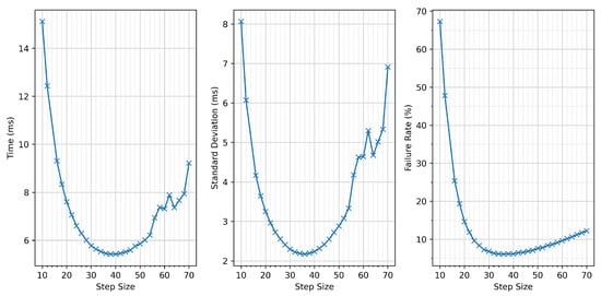
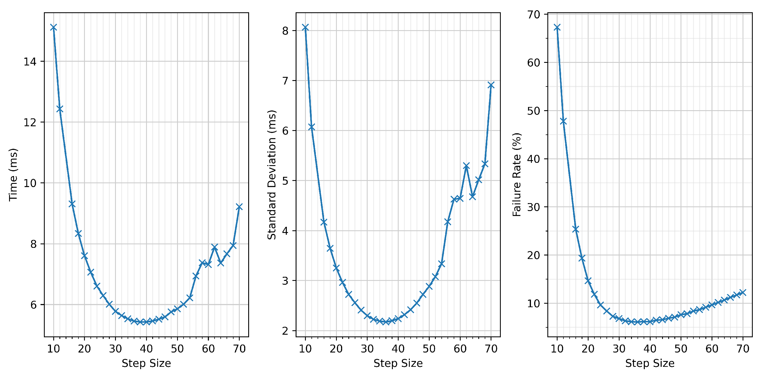
Coordinate Descent (CD) also relies on a fixed step size, but unlike Gradient Descent, it optimises only a single EPC control voltage at a time. This restriction to one-dimensional search directions makes the method simple, lightweight, and often effective when the response landscape is highly nonlinear. To determine an appropriate step size, we performed a sweep over values from 10 to 70 (inclusive), using increments of 2. For each step size, $500,000$ initial alignment trials were simulated, and the average optimisation time, standard deviation, and failure rate were recorded. The results are shown in Figure 4.

Figure 4. Performance of Coordinate Descent for step sizes between 10 and 70 (in increments of 2), using 500,000 simulated initial-alignment trials per point. (left): average optimisation time; (centre): standard deviation; (right): failure rate. A step size of 36 provides the best trade-off between convergence speed and reliability.

The failure-rate trend is qualitatively similar to that observed for Gradient Descent: both excessively small and excessively large step sizes increase the likelihood of the algorithm becoming trapped above the acceptance threshold. For small step sizes, convergence slows, and the method becomes susceptible to shallow local minima and saddle regions. For large step sizes, the algorithm reaches the vicinity of the optimum quickly but lacks the precision required to refine the solution to within the $0.01$ rad tolerance, causing premature termination.

The optimisation-time curve exhibits a minimum at a step size of 38. Below this value, convergence slows for the same reason as in Gradient Descent—steps are simply too small to traverse the fitness landscape efficiently. Above this value, the optimisation time increases again; here, the algorithm must rely on noise-induced perturbations to recover from overshooting or misalignment introduced by large steps, adding unnecessary delay.

For subsequent algorithm comparisons, we selected a step size of 36, which provides the lowest failure rate with a negligible difference in average optimisation time. This choice achieved an average optimisation time of $5.456\mathrm{ms}$, a standard deviation of $2.172\mathrm{ms}$, and a failure rate of $6.094\%$ (rounded to three decimal places).

4.4. Simulated Annealing

Simulated Annealing (SA) requires selecting two hyperparameters: the initial temperature and the cooling coefficient that determines how quickly the temperature decreases. At every iteration, the temperature is updated using a multiplicative cooling schedule of the form

$$T^{\prime }=cT,$$

where $0<c<1$ is the cooling coefficient. Faster cooling (smaller c) reduces the number of high-temperature iterations that can escape local minima but may prevent the algorithm from sufficiently refining its solution. Conversely, slow cooling improves reliability but increases optimisation time.

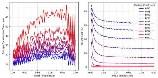
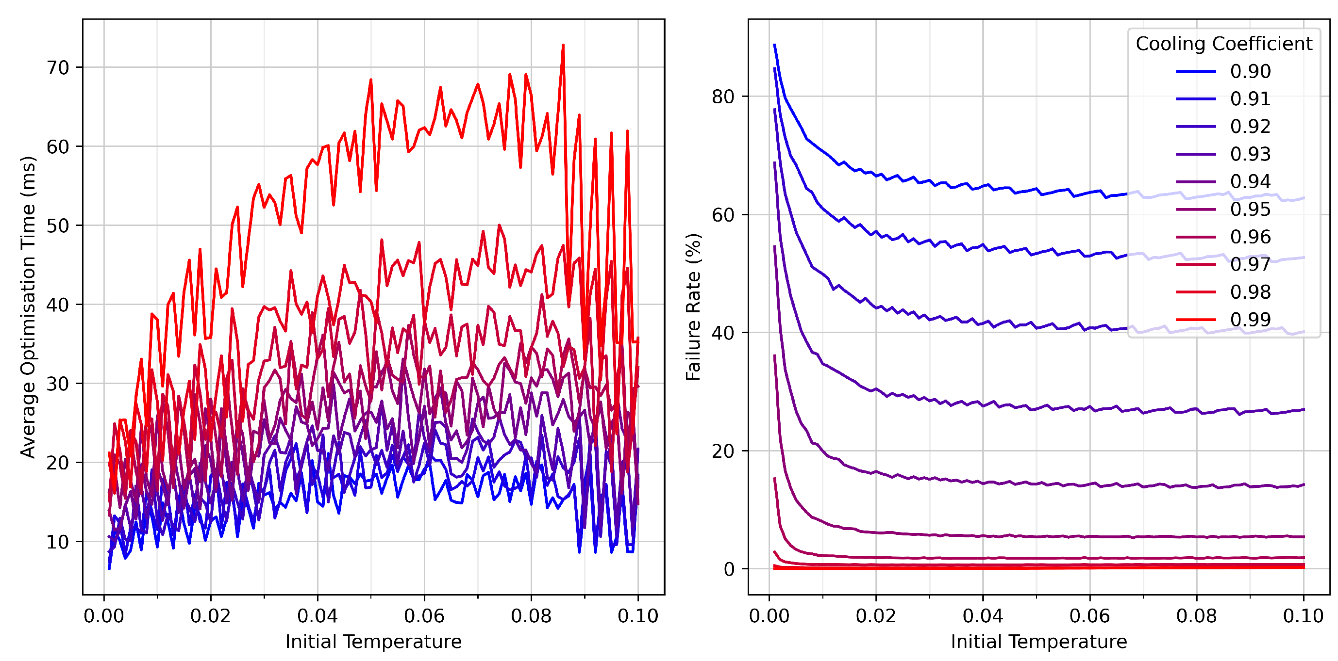
To identify suitable values for these parameters, we performed a two-dimensional sweep: the initial temperature was varied from $0.001$ to $0.1$ in increments of $0.001$, and the cooling coefficient from $0.90$ to $0.99$ in increments of $0.01$. For each parameter pair, $500,000$ initial-alignment trials were run. The resulting average optimisation times and failure rates are presented in Figure 5.

Figure 5. Simulated Annealing performance as a function of initial temperature and cooling coefficient. (left): average optimisation time; (right): failure rate. Each data point represents 500,000 simulated initial-alignment trials. Low initial temperature and fast cooling lead to rapid convergence but higher failure probability, whereas slower cooling achieves a near-zero failure rate.

Inspection of these results reveals clear trends. Both the initial temperature and cooling coefficient are positively correlated with the average optimisation time; high initial temperature or slowly cooled schedules produce more exploratory behaviour, resulting in longer convergence. However, the failure rate places more stringent constraints on the choice of parameters. Low initial temperatures or aggressive cooling schedules (small c) cause the algorithm to “freeze” too early, reducing its ability to escape local minima and dramatically increasing the failure rate. The only parameter combinations achieving a failure rate below $1\%$ were those with $c=0.98$ or above, or $c=0.97$ with initial temperature $\ge 0.004$.

Balancing exploration time and success probability, we selected an initial temperature of $0.005$ with a cooling coefficient of $0.99$ for the algorithm comparison. This choice provides a high reliability (0% failure rate in the later comparison) while keeping the optimisation time competitive with the other algorithms. Although slower than Coordinate Descent and Adaptive Gradient Descent, Simulated Annealing’s robustness to local minima makes it a valuable tool for both initial alignment and, especially, realignment tasks in continuous control scenarios.

4.5. Comparison of Algorithms

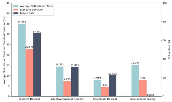
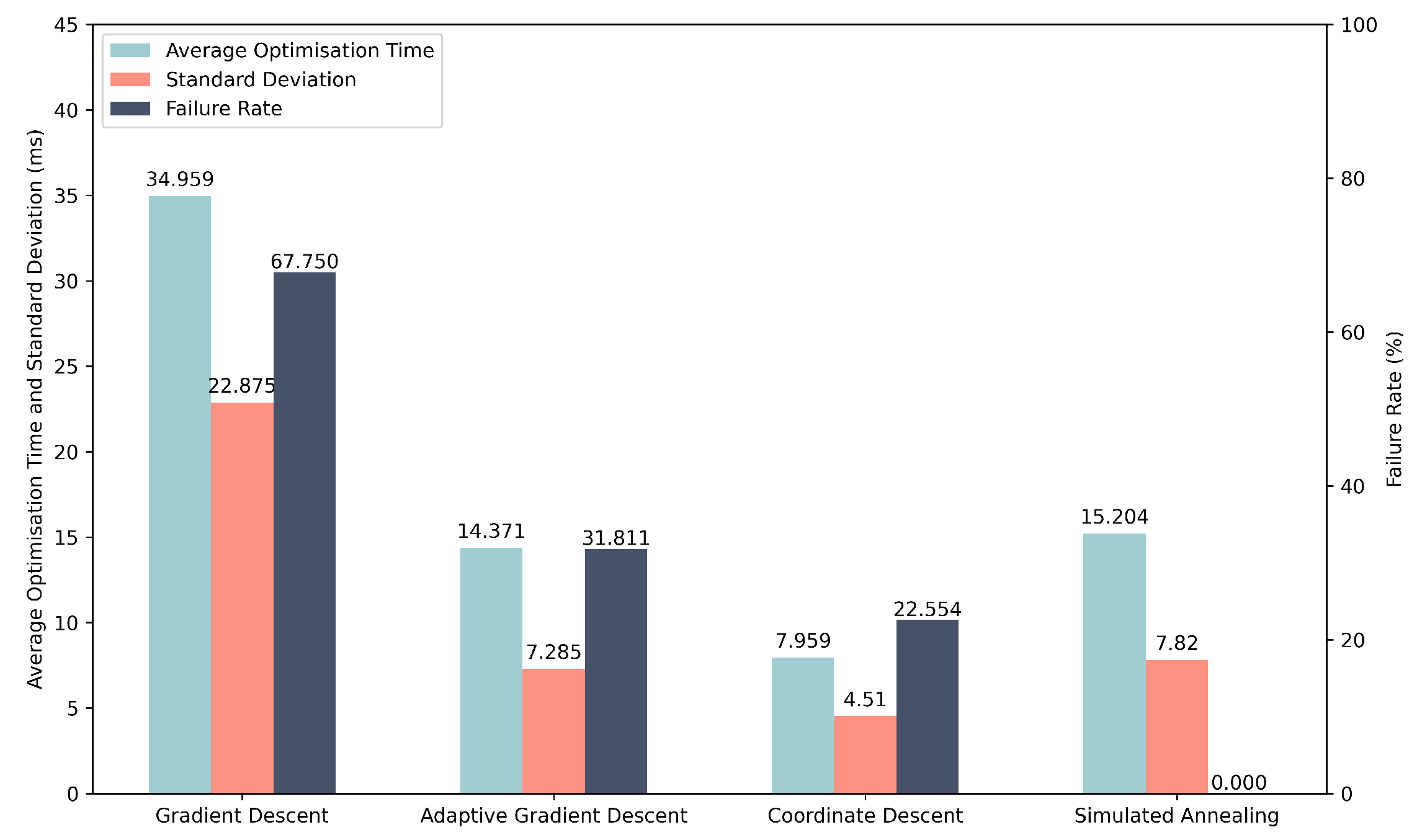
To compare the overall performance of the four optimisation algorithms, we conducted a large-scale simulation campaign consisting of one million trials. In each trial, all algorithms were presented with the same initial conditions: a random EPC voltage vector and a random polarisation misalignment produced by the channel model. This ensures that performance differences arise solely from the optimisation strategies themselves. The resulting average optimisation times, standard deviations, and failure rates are summarised in Table 1, with corresponding bar plots shown in Figure 6.

Table 1. Simulated performance of the four optimisation algorithms using 1,000,000 shared initial conditions. Reported metrics include the average optimisation time, standard deviation, and failure rate. All values are rounded to three decimal places.

Algorithm	Average Optimisation Time (ms)	Standard Deviation (ms)	Failure Rate
Gradient Descent	34.959	22.875	67.750%
Adaptive Gradient Descent	14.371	7.285	31.811%
Coordinate Descent	7.959	4.510	22.554%
Simulated Annealing	15.204	7.820	0.000%

Figure 6. Simulated performance comparison of the four optimisation algorithms over 1,000,000 trials. Error bars indicate standard deviation. Simulated Annealing achieves perfect reliability, whereas Coordinate Descent provides the fastest average optimisation time.

The results clearly validate the qualitative hypotheses proposed at the beginning of this section. Coordinate Descent is the fastest algorithm, achieving an average optimisation time of approximately 8.0 ms, outperforming the other Gradient Descent variants. Its axis-aligned updates allow it to locate improving directions with relatively few fitness evaluations. However, this speed comes with a non-zero failure rate of around 22.6%, indicating that CD can still become trapped in local minima.

Adaptive Gradient Descent performs substantially better than fixed step-size Gradient Descent in both speed and reliability, reducing the failure rate from 67.8% to about 31.8%. This demonstrates the effectiveness of scaling the step size with the fitness value: large steps enable rapid early progress, while smaller steps facilitate precise refinement near the target state.

Simulated Annealing stands out for its reliability. With the chosen hyperparameters, SA achieved a 0% failure rate across all one million trials. This reflects its ability to escape local minima through probabilistic acceptance of worse solutions at high temperature. The cost of this robustness is a longer average optimisation time of about 15.2 ms, slower than Coordinate Descent and Adaptive Gradient Descent, but still faster than fixed step-size Gradient Descent.

Taken together, these results highlight a clear trade-off between speed and reliability. Coordinate Descent is the preferred choice for rapid initial alignment, whereas Simulated Annealing delivers unmatched stability and is therefore well suited for realignment tasks in continuous polarisation control.

4.6. Continuous Polarisation Control

We now consider how the optimisation algorithms can be used not only for initial polarisation alignment but also for continuous polarisation control in the presence of drift. In this setting, the system operates near a target state most of the time, and realignment is triggered only when the polarisation error exceeds a specified tolerance.

Once the fitness value rises above a chosen threshold, a realignment procedure is invoked to drive the state back into the acceptable region around the target. In our simulations, we set this threshold at $f=0.05$ (corresponding to a QBER of $0.0629\%$), but in practice it can be tuned to reflect the maximum tolerable QBER for a given QKD deployment.

For initial alignment, we employ Coordinate Descent because it offers the lowest average optimisation time among the algorithms tested. If CD fails to find a solution below the acceptance threshold, the EPC voltages are reinitialised to random values and the procedure is restarted. This strategy is acceptable at start-up, when no prior information is available, and occasional restarts are not disruptive.

For realignment during continuous operation, however, failures are more costly: if the algorithm cannot restore alignment, the only fallback is to randomise the EPC inputs and repeat the initial alignment procedure, leading to extended downtime. To minimise this risk, we use Simulated Annealing for realignment. Although SA has a higher average optimisation time than Coordinate Descent when started from random initial conditions, in the continuous-control regime, it begins from a relatively low fitness value (just above the threshold around $f\approx 0.05$). In this regime, the longer convergence time is less critical, while the near-zero failure rate of SA becomes a decisive advantage. A representative example of this hybrid strategy—initial alignment with Coordinate Descent, followed by drift and subsequent realignment with Simulated Annealing—is shown in Figure 7.

Figure 7. Simulated initial alignment and continuous polarisation control over a 10 s interval. Red segments indicate periods during which an optimisation algorithm is active; blue segments denote free evolution (F.E.). The light blue horizontal line marks the acceptance threshold ($\alpha =0.01$), and the orange line marks the realignment threshold ($\alpha =0.05$). The inset highlights the realignment dynamics achieved by Simulated Annealing (S.A.).

It is important to emphasise that realignment constitutes a different optimisation problem from initial alignment: instead of starting from a random point on the Poincaré sphere, the algorithm begins close to the target state. Consequently, the hyperparameter settings for Simulated Annealing that were optimised for the initial-alignment tests are not necessarily optimal for this regime. When generating Figure 7, the initial temperature and cooling coefficient were adjusted by trial and error to yield satisfactory performance. A more systematic optimisation of these parameters for continuous control could be carried out in future work, but simple manual tuning was sufficient for the purposes of demonstration.

Having seen encouraging results from the simulated optimisation algorithms, we next assess their performance in the experimental setup described in Section 2.3.

5. Experimental Results

To assess how the optimisation algorithms perform under real operating conditions, we repeated the procedure of hyperparameter testing, algorithm comparison, and continuous-control demonstration using the experimental setup described in Section 2.3. While simulations provide valuable qualitative insight, they necessarily rely on simplified models of the EPC and channel. The experimental results therefore serve two purposes: (i) to validate which features of the simulated behaviour transfer to a real system, and (ii) to identify discrepancies that arise from physical effects not captured in the simulation framework.

Although hyperparameter tuning was already carried out in simulation, repeating this process experimentally is essential. Real EPCs exhibit nonlinear voltage–retardance responses, mechanical hysteresis, cross-coupling between channels, and device-specific idiosyncrasies. Similarly, the experimental polarisation drift differs from the idealised random-walk model used in simulation, as shown earlier in Figure 1b. For these reasons, the optimal hyperparameters for each optimisation algorithm must be determined independently in the laboratory. All hyperparameter tests reported below were performed in the “state-generation” configuration, i.e., without the 50 km fibre spool, allowing many repetitions in a stable and controlled environment.

Our qualitative hypotheses for expected performance remain the same as in the simulated study. However, due to the additional complexity and imperfections of the real system, we entered the experimental stage with less confidence that the same trends—especially relative magnitudes of convergence times and failure rates—would persist. As will be seen, some algorithms behave similarly to their simulated counterparts, while others differ substantially.

In the subsections that follow, we present the experimental hyperparameter testing for each algorithm, followed by a comparison using the best-performing settings, and finally a demonstration of continuous polarisation control over a two-hour interval with real fibre-induced drift.

5.1. Gradient Descent

For the experimental implementation of Gradient Descent, we performed a sweep over the fixed step size to determine a suitable operating point. Unlike in simulation—where the EPC model is idealised and noise-free—the real EPC exhibits nonlinear voltage–retardance behaviour, hysteresis, and channel cross-coupling. As a result, the optimal step size cannot be inferred from simulation and must be obtained empirically.

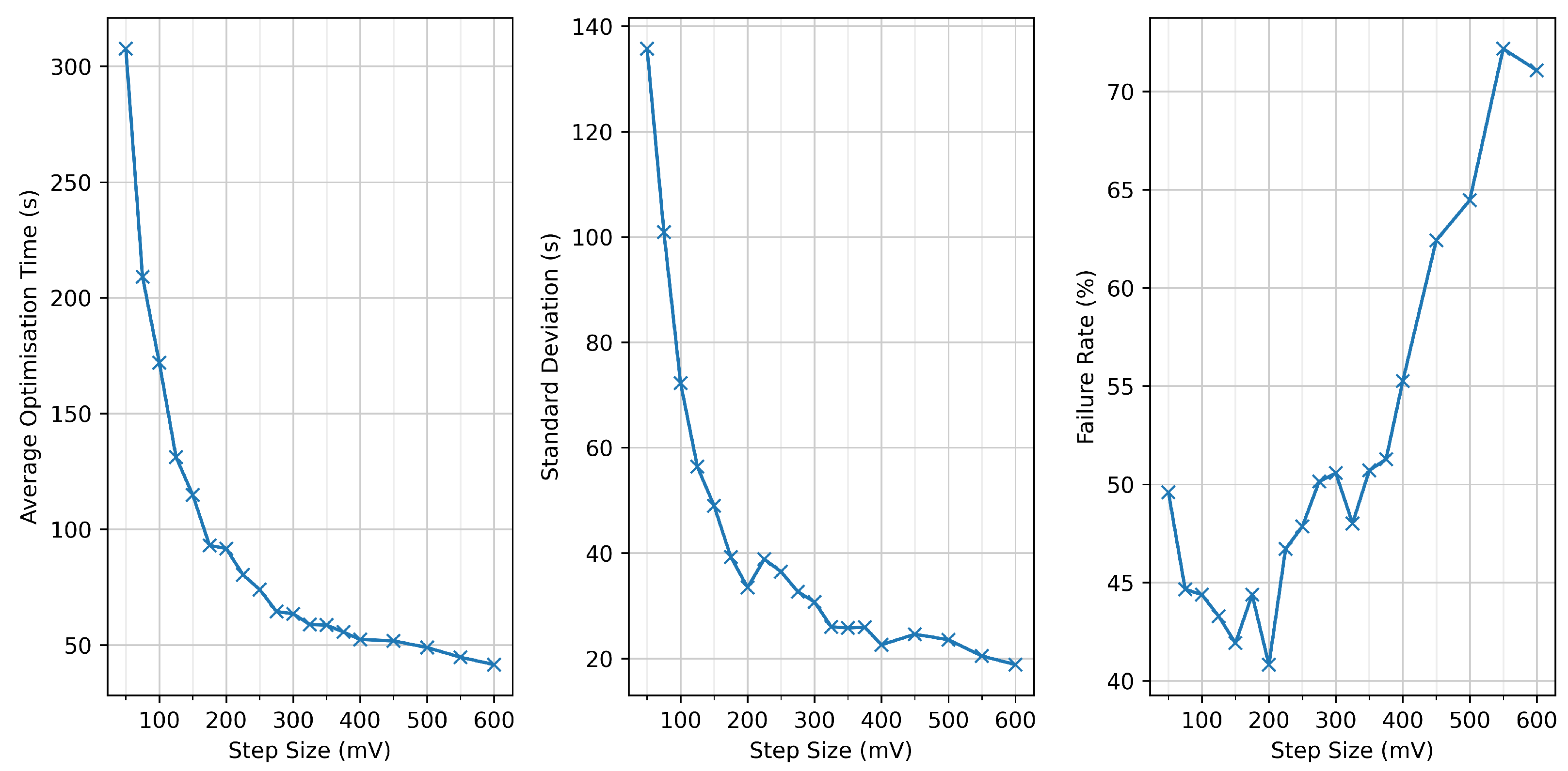
We tested step sizes ranging from $25\mathrm{mV}$ to $400\mathrm{mV}$ in increments of $25\mathrm{mV}$, and from $450\mathrm{mV}$ to $600\mathrm{mV}$ in increments of $50\mathrm{mV}$. For each value, we repeatedly initialised the EPC with random voltages and measured the resulting average optimisation time, standard deviation, and failure rate. The results are summarised in Figure 8.

Figure 8. Experimental performance of Gradient Descent for step sizes between 50 mV and 600 mV. (left): average optimisation time; (centre): standard deviation; (right): failure rate. Step sizes from 25–$400\mathrm{mV}$ (in $25\mathrm{mV}$ increments) and 450–$600\mathrm{mV}$ (in $50\mathrm{mV}$ increments) were evaluated. The trade-off between optimisation time and reliability indicates that 350 mV offers a favourable balance between convergence speed and reliability.

The behaviour observed experimentally mirrors the trends found in simulation. Larger step sizes systematically reduce the average optimisation time, as the algorithm traverses the voltage space more rapidly. However, the failure rate increases sharply beyond a certain point: excessively large steps overshoot the basin of attraction around the target state, preventing the algorithm from achieving the required angular precision before stalling.

Conversely, very small step sizes yield low failure rates but slow convergence, as the algorithm must take many fine steps to approach the optimum. Between these extremes lies a favourable operating region, and from the data we identified $350\mathrm{mV}$ as a suitable compromise. At this setting, the algorithm achieved an average optimisation time of $58.603\mathrm{s}$, a standard deviation of $25.796\mathrm{s}$, and a failure rate of $50.710\%$ (all rounded to three decimal places). Although the failure rate remains high compared to simulation, this step size minimises runtime without sacrificing additional reliability.

The substantial discrepancy between the simulated and experimental failure rates highlights the sensitivity of Gradient Descent to practical EPC nonlinearities and measurement noise—factors not fully captured by the idealised model used in Section 2.

5.2. Adaptive Gradient Descent

For the experimental implementation of Adaptive Gradient Descent, we retained the same fitness-dependent step-size schedule used in simulation. The rationale behind this scheme—large steps when far from the target, smaller steps when close—remains valid when operating a real EPC, whose nonlinear and device-specific response makes the choice of a single globally optimal step size impractical.

Recall that the adaptive schedule is defined as

$$S\left(f\right)=200\sqrt{f},$$

where f is the current fitness value. This function preserves large step sizes over a broad region of the search space, enabling rapid coarse alignment, while ensuring that steps decrease smoothly as the target state is approached.

To characterise the algorithm’s performance experimentally, we executed Adaptive Gradient Descent continuously for 24 h, repeatedly initialising the EPC with random voltages. Over this dataset, the algorithm achieved an average optimisation time of $202.668\mathrm{s}$, with a standard deviation of $56.070\mathrm{s}$, and a failure rate of $43.101\%$ (all rounded to three decimal places).

These results differ markedly from the simulated performance presented in Section 4, where Adaptive Gradient Descent outperformed its fixed-step counterpart. In the experiment, the adaptive schedule yields a lower failure rate than standard Gradient Descent, but at the cost of significantly longer convergence times, nearly an order of magnitude slower on average. We attribute this to two factors:

• The real EPC exhibits nonlinear, asymmetric, and occasionally hysteretic voltage–retardance behaviour, causing the effective step size to vary unpredictably for a given fitness value.
• Measurement noise and slow drift in the experimental setup affect fitness evaluations, particularly near the target state, where the adaptive mechanism reduces step sizes aggressively.

These effects collectively flatten the progress of the algorithm during the refinement phase, causing long optimisation tails. Consequently, while the adaptive strategy improves robustness relative to fixed step-size Gradient Descent, it becomes less suitable for rapid initial alignment in practical QKD systems.

5.3. Coordinate Descent

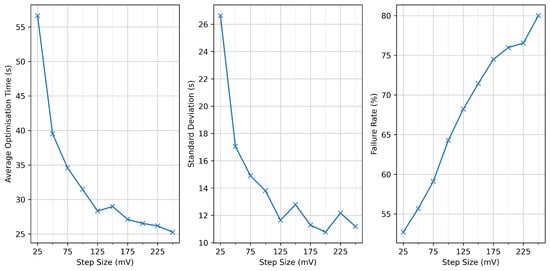
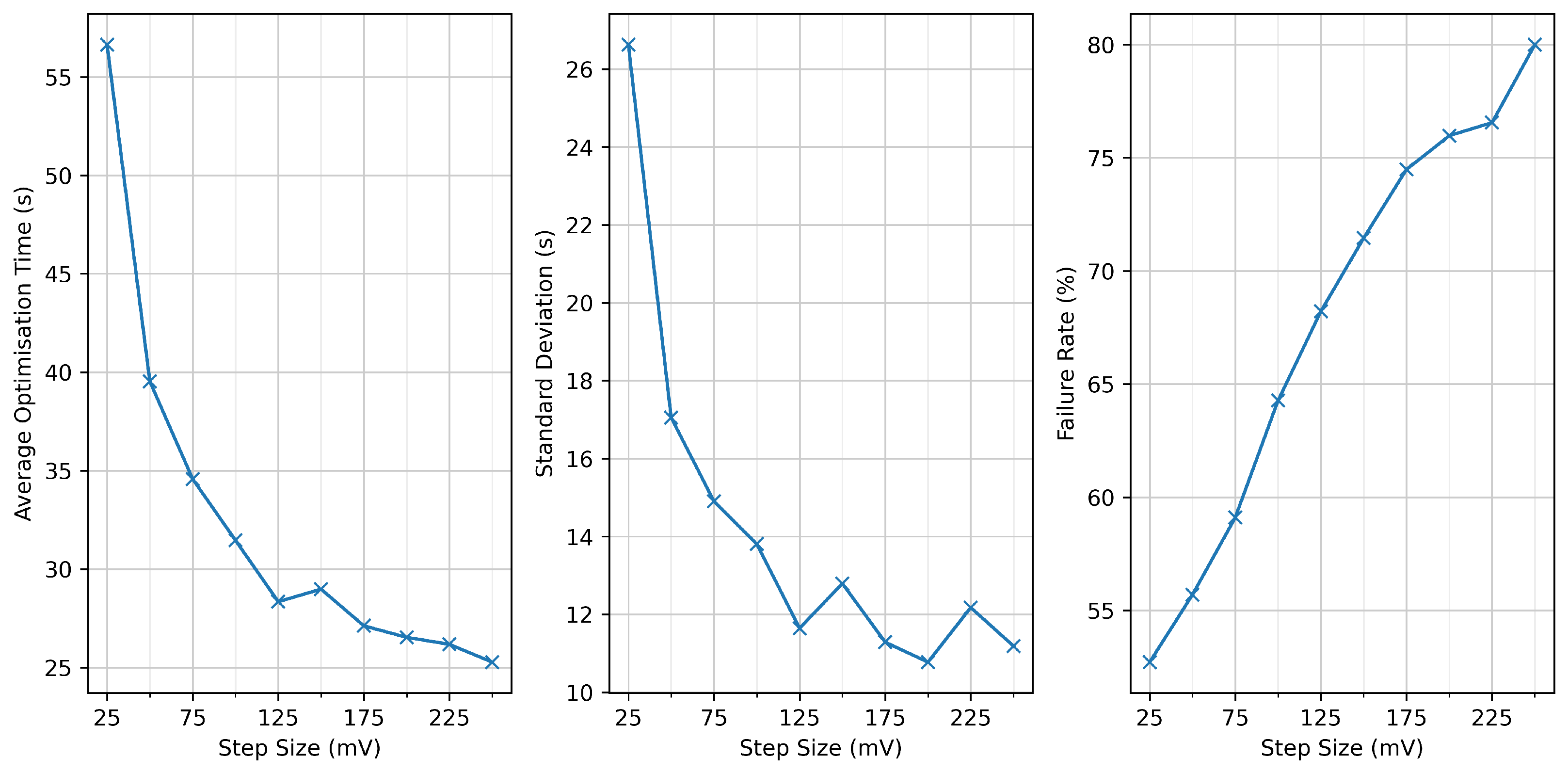
For the experimental implementation of Coordinate Descent, we performed a sweep over step sizes ranging from $25\mathrm{mV}$ to $250\mathrm{mV}$ in increments of $25\mathrm{mV}$. For each value, the algorithm was repeatedly initialised with random EPC voltages, and the resulting average optimisation time and failure rate were recorded. The results are shown in Figure 9.

Figure 9. Experimental performance of Coordinate Descent for step sizes between 25 mV and 250 mV. Average optimisation time decreases with step size, and failure rate increases.

The behaviour observed in the experiment is partly consistent with the simulated results presented in Section 4. In both cases, the average optimisation time exhibits a well-defined minimum for intermediate step sizes, reflecting the standard trade-off: small steps slow convergence, while excessively large steps prevent fine-grained refinement near the target state.

However, the failure-rate behaviour differs substantially from that seen in simulation. Whereas the simulated Coordinate Descent exhibited an optimal step size that minimised the failure rate, the experimental implementation shows a monotonic increase in failure rate across the entire tested range. This degradation is likely due to practical imperfections not modelled in simulation, including:

• Nonlinear voltage–retardance response: large step sizes may overshoot fine features of the EPC response curve, while small step sizes may be insufficient to overcome measurement noise when refining the solution.
• Axis misalignment and channel coupling: real EPC stages are not perfect waveplates, and adjusting one voltage can inadvertently affect multiple effective polarisation components.
• Measurement noise: small improvements may be masked by polarimeter noise, causing the coordinate selection rule to choose suboptimal directions or stall prematurely.

Balancing these effects, we selected a step size of $75\mathrm{mV}$ for use in the cross-algorithm comparison. This value provides a favourable compromise between fast optimisation and a tolerable failure rate. At this operating point, Coordinate Descent achieves an average optimisation time of $34.573\mathrm{s}$, with a standard deviation of $14.903\mathrm{s}$, and a failure rate of $59.107\%$ (rounded to three decimal places).

Despite its higher failure rate in experiment, the speed advantage of Coordinate Descent makes it well suited for initial alignment, where rapid convergence is more critical than absolute reliability and failed runs can be recovered by reinitialising the EPC inputs.

5.4. Simulated Annealing

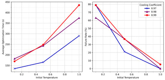
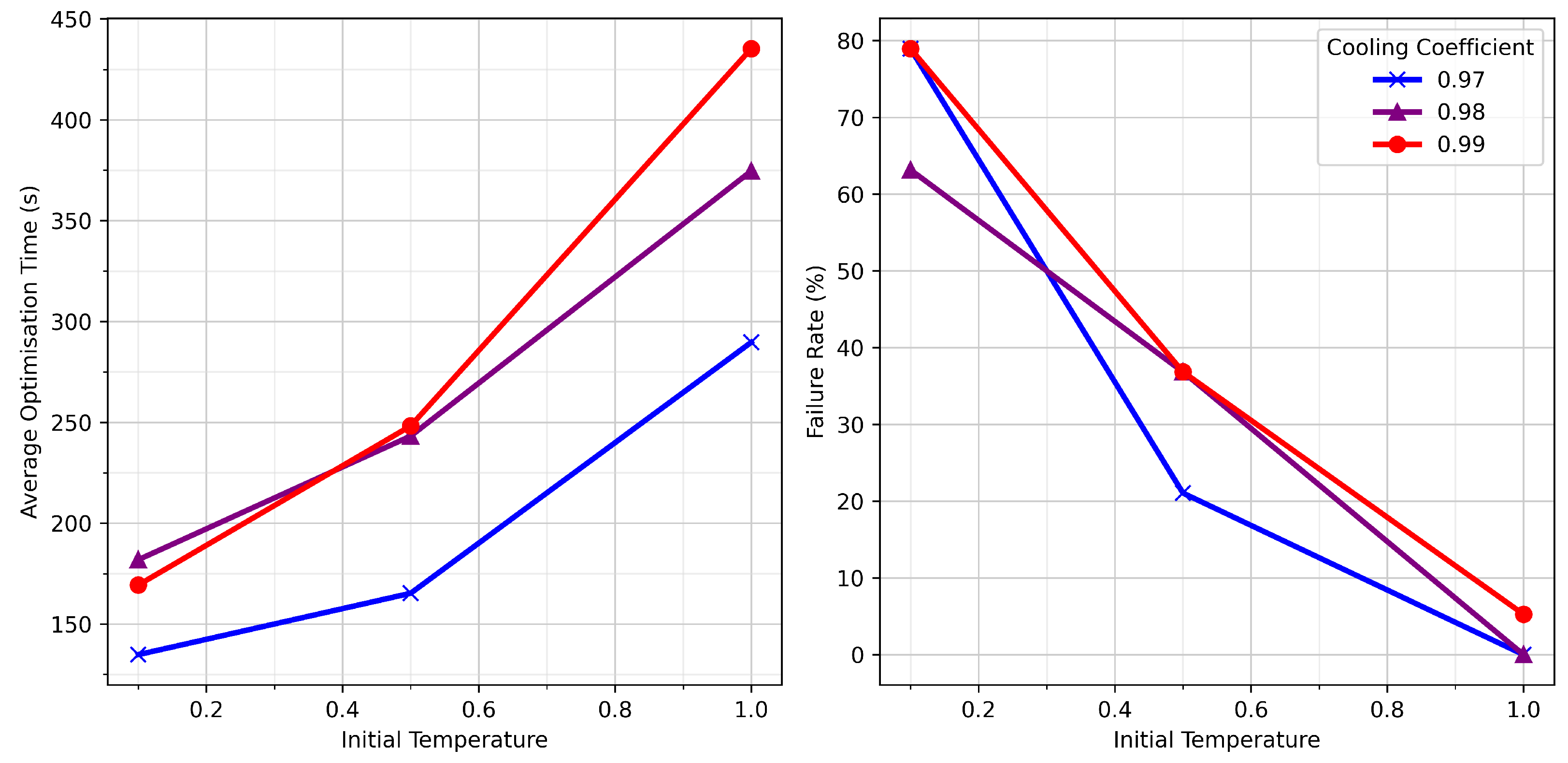
For the experimental implementation of Simulated Annealing (SA), we evaluated a small grid of hyperparameter settings. Specifically, we tested cooling coefficients of $0.99$, $0.98$, and $0.97$, and initial temperatures of $0.10$, $0.50$, and $1.00$. For each parameter pair, the optimisation was repeatedly initialised from random EPC voltages over a 24 h data collection period. The resulting average optimisation times and failure rates are shown in Figure 10.

Figure 10. Experimental performance of Simulated Annealing for combinations of initial temperature and cooling coefficient. (left): average optimisation time; (right): failure rate. Cooling coefficients of 0.97–0.98 with an initial temperature of 1.0 yield a near-zero failure rate. Results were gathered over a 24 h experimental run.

The trends observed experimentally mirror those seen in simulation. In particular, the following:

• Slower cooling (larger $\mathit{c}$) enables more extensive exploration, improving reliability but increasing optimisation time.
• Higher initial temperatures similarly increase the probability of accepting uphill moves and therefore reduce failure rates.

Only two hyperparameter combinations achieved failure rates close to $0\%$: an initial temperature of $1.00$ combined with cooling coefficients of $0.97$ or $0.98$. Between these two settings, $c=0.97$ yielded the shorter average optimisation time, and was therefore adopted for our cross-algorithm comparison.

Under this configuration, SA achieved an average optimisation time of $289.676\mathrm{s}$ with a standard deviation of $82.239\mathrm{s}$ (rounded to three decimal places), and a failure rate of $0\%$.

Although Simulated Annealing is noticeably slower than the other optimisation methods in the experimental setting—significantly slower, for instance, than Gradient Descent or Coordinate Descent—its perfect reliability makes it uniquely well suited for situations where failures are unacceptable. As we discuss later, this property motivates its use in our continuous-control strategy, where a failed realignment would trigger a full reinitialisation of the EPC, causing substantial downtime.

5.5. Comparison of Algorithms

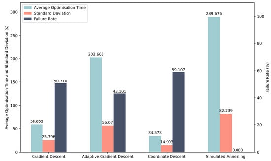
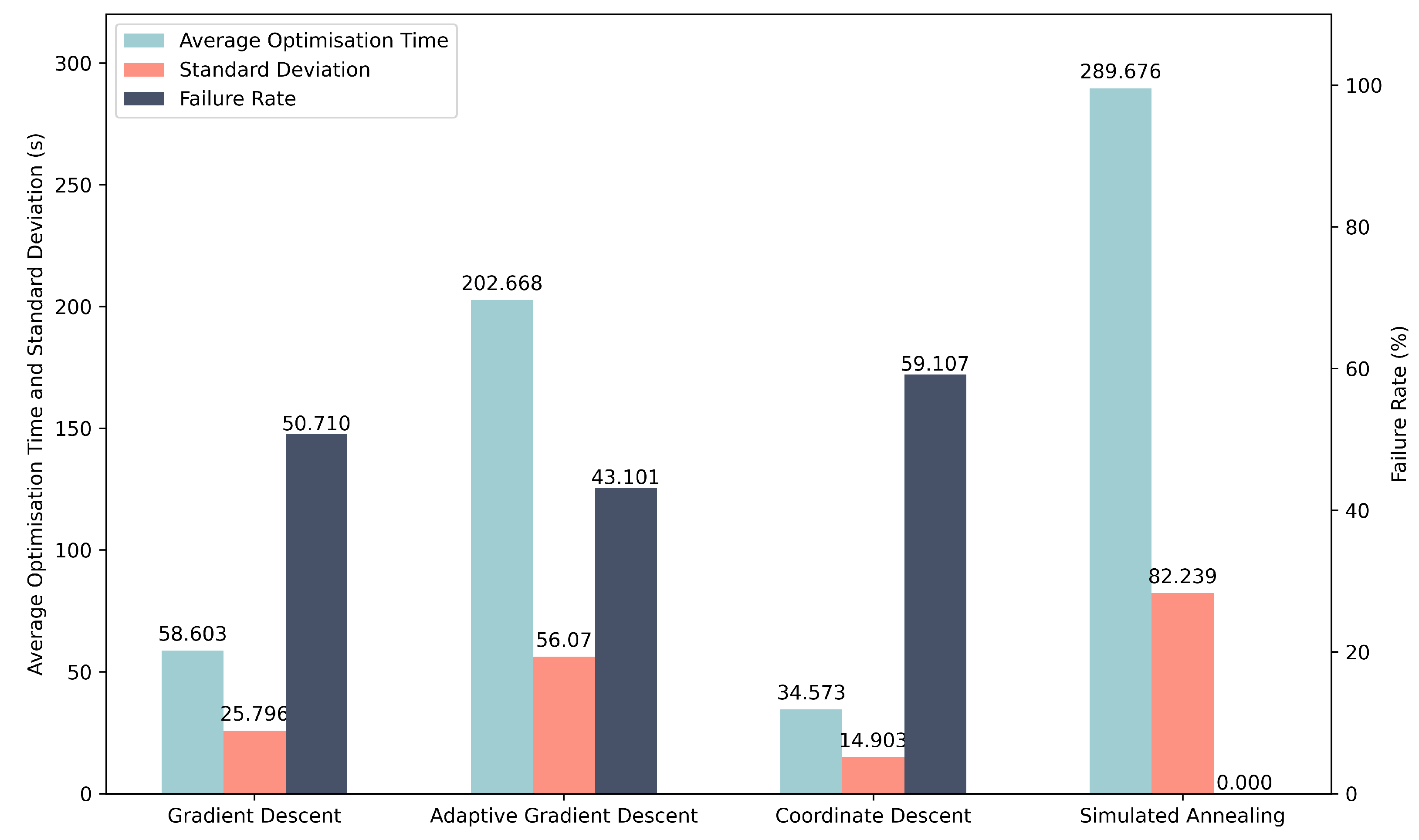
Because experimental data acquisition is significantly more time-consuming than simulation, we used the results obtained during the hyperparameter testing phase as the basis for comparing the performance of the four optimisation algorithms. Each algorithm was evaluated using its selected hyperparameters, as justified in the preceding subsections. The resulting average optimisation times, standard deviations, and failure rates are summarised in Table 2 and visualised in Figure 11.

Table 2. Experimental performance of the four optimisation algorithms. Metrics are taken from the best-performing hyperparameter settings identified during the sweep. All values are rounded to three decimal places.

Algorithm	Average Optimisation Time (s)	Standard Deviation (s)	Failure Rate
Gradient Descent	58.603	25.796	50.710%
Adaptive Gradient Descent	202.668	56.070	43.101%
Coordinate Descent	34.573	14.903	59.107%
Simulated Annealing	289.676	82.239	0.000%

Figure 11. Experimental comparison of the four optimisation algorithms using the optimal hyperparameters identified in the individual sweeps. Simulated Annealing achieves perfect reliability, while Coordinate Descent provides the fastest average optimisation time.

These results broadly reflect the qualitative trends observed in simulation but also reveal notable divergences arising from the increased complexity of the physical EPC and fibre system.

First, although Adaptive Gradient Descent outperformed fixed-step Gradient Descent in simulation, the experimental results show the opposite behaviour: AGD requires a significantly longer optimisation time, despite achieving a moderately improved failure rate. This inversion suggests that the assumed smoothness of the simulated voltage–polarisation landscape does not fully capture the nonlinearities, cross-coupling, and hysteresis present in the real EPC.

Second, while Coordinate Descent remains the fastest method on average—as hypothesised—the experimental failure rate is unexpectedly higher than that of either Gradient Descent or Adaptive Gradient Descent. This contrasts with the simulation results, in which CD was both fast and reliable. The increased failure rate may stem from strong channel–voltage coupling and non-axis-aligned valleys in the true fitness landscape, which limit the effectiveness of strictly coordinate-aligned updates.

Simulated Annealing, by contrast, maintains its key strength: a **0% failure rate**. Although its optimisation time is substantially longer than in simulation, its perfect reliability remains highly attractive for realignment tasks where optimisation failure would require a costly EPC reset.

Overall, the experimental comparison reinforces the complementary nature of the algorithms: Coordinate Descent excels in speed, while Simulated Annealing excels in robustness. These findings motivate the hybrid control strategy used in our continuous polarisation tracking experiments.

5.6. Continuous Polarisation Control

Finally, we evaluated the ability of the optimisation algorithms to maintain a stable polarisation state under realistic long-term channel drift. As in the simulation study, we used a hybrid control strategy: Coordinate Descent (CD) performs the initial alignment due to its fast convergence, while Simulated Annealing (SA) performs realignment whenever the angular error exceeds a predefined threshold. The rationale mirrors that of Section 4: initial alignment benefits from speed, whereas realignment demands robustness to avoid repeated EPC resets.

To generate sufficient drift for meaningful testing, a $50\mathrm{km}$ ultra-low-loss single-mode fibre spool was inserted between the VOA and the polarimeter. Environmental fluctuations—primarily temperature changes and mechanical relaxation of the fibre—produce slow, stochastic polarisation drift over the two-hour acquisition period.

The fitness threshold for triggering realignment was set to $\alpha =0.05$ rad (corresponding to a QBER of $0.0625\%$), while convergence was defined as achieving $\alpha \le 0.01$ rad. These thresholds match those used in the simulation study, facilitating direct comparison across both domains.

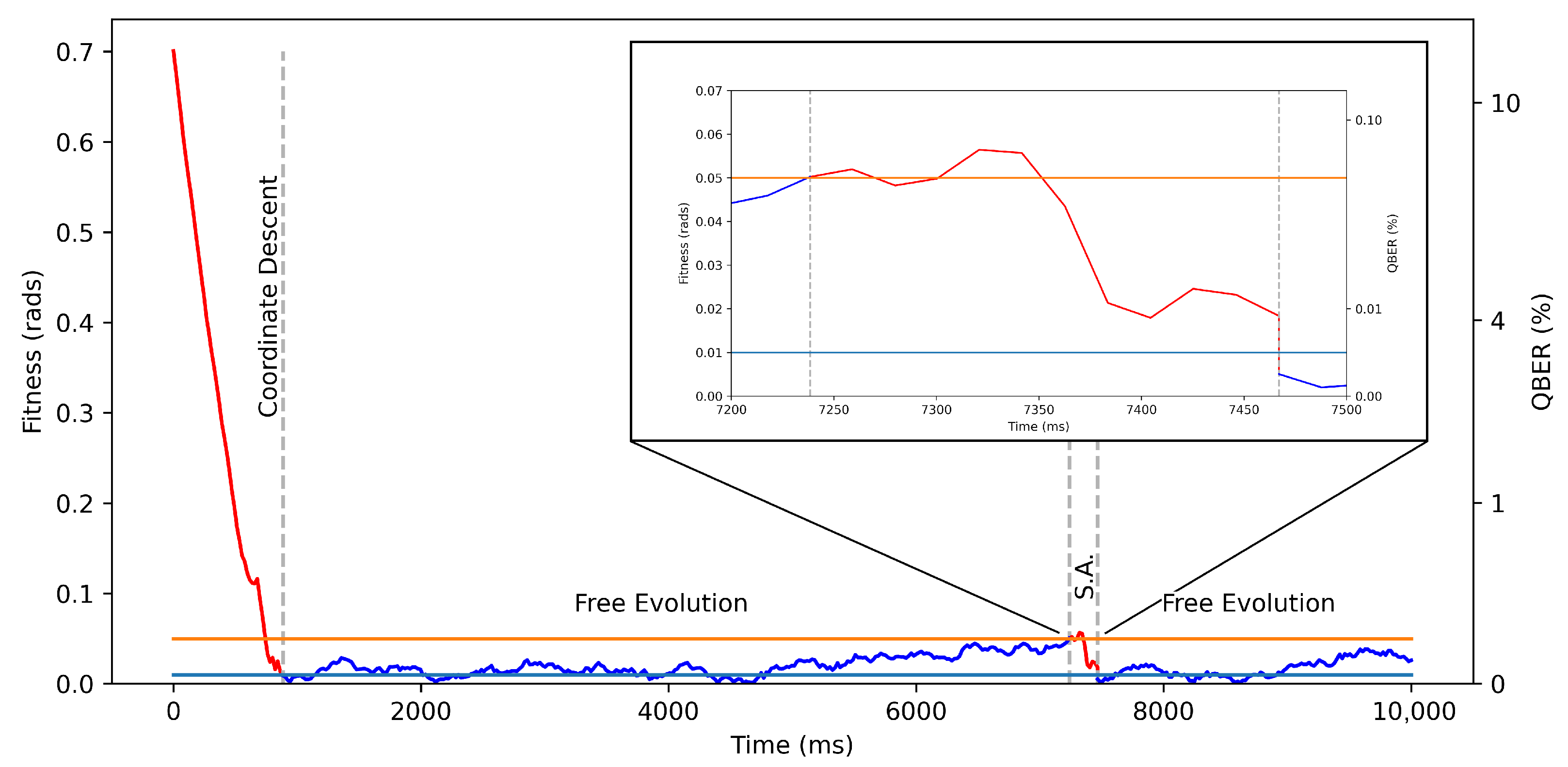
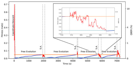
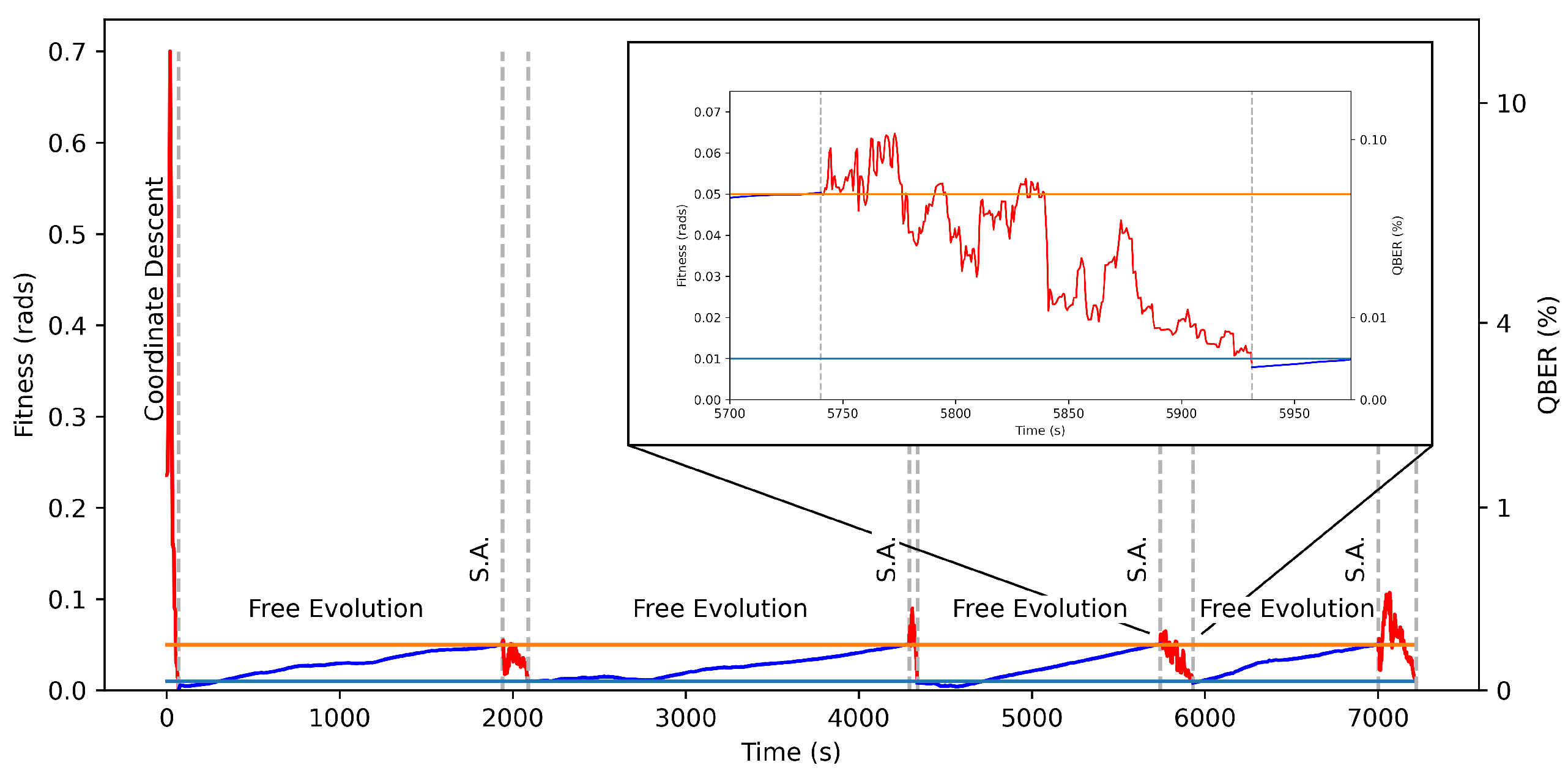
Figure 12 shows the evolution of the angular error over the full two-hour run. Intervals during which an optimisation algorithm is active are highlighted in red, while periods of free drift are shown in blue. Each realignment episode successfully drives the error back below the acceptance threshold, demonstrating that the combination of CD (for fast initial alignment) and SA (for reliable realignment) can maintain stable polarisation tracking over extended durations without manual intervention.

Figure 12. Experimental initial alignment and continuous polarisation control over a 2-h period. Red segments indicate periods when an optimisation algorithm is active; blue segments represent free evolution. Realignment is triggered when the fitness exceeds $\alpha =0.05$ (orange line), and convergence is declared at $\alpha =0.01$ (light blue line). The inset illustrates a typical realignment event.

The overall behaviour closely mirrors the simulated results, though real-world drift exhibits larger excursions and slower characteristic timescales than those generated by the simple random-walk model. Despite these differences, the hybrid scheme remains effective, underscoring its suitability for deployment in QKD receivers where long-term stability and unattended operation are essential.

6. Conclusions and Further Work

We have presented a systematic comparison of four optimisation algorithms for electronic polarisation control in fibre-based Quantum Key Distribution systems. Using both a numerical EPC model and a fibre-based experimental platform, we evaluated Gradient Descent, Adaptive Gradient Descent, Coordinate Descent, and Simulated Annealing in terms of convergence speed, stability, and reliability. This constitutes, to our knowledge, the first side-by-side benchmark of these algorithms under conditions representative of practical QKD operation.

Our simulation results confirm clear performance differences between the algorithms. Coordinate Descent exhibited the fastest convergence (average 2.10 ms), while Simulated Annealing was the only algorithm to achieve a perfect success rate. Adaptive Gradient Descent improved upon fixed step-size Gradient Descent in both speed and reliability, but remained inferior to Coordinate Descent. These trends reflect the structure of the EPC control landscape: Coordinate Descent efficiently exploits the local geometry of the space, whereas Simulated Annealing excels at escaping local minima.

The experimental results reproduce the qualitative behaviour observed in simulation, though with important quantitative differences arising from real-world device nonlinearities and fibre-induced drift. Coordinate Descent again yielded the fastest average alignment time (34.6 s), while Simulated Annealing maintained its perfect reliability. In contrast, Adaptive Gradient Descent performed less favourably than expected, exhibiting slower convergence than fixed step-size Gradient Descent, an outcome likely linked to the more complex and state-dependent voltage–retardance behaviour of the EPC compared to the idealised simulation model.

Leveraging these insights, we implemented a hybrid control strategy combining the strengths of both algorithms: Coordinate Descent for rapid initial alignment, followed by Simulated Annealing for high-reliability realignment during continuous operation. This hybrid method was tested experimentally over a two-hour interval with a 50 km drifting fibre channel. The system successfully maintained the target polarisation state without manual intervention, demonstrating a practical path toward autonomous polarisation tracking in deployed QKD receivers.

Future Work

Our study highlights several promising directions for further research. First, improved physical models of EPC behaviour accounting for axis misalignment, nonlinear voltage–retardance responses, and inter-channel coupling, which could greatly enhance simulation fidelity and guide the development of more refined optimisation strategies. Second, the observed deviation between experimental drift patterns and the standard random-walk model suggests the need for updated theoretical descriptions of long-fibre polarisation evolution. Third, the design of adaptive or learning-based step-size schedules, potentially discovered via genetic programming or reinforcement learning, may yield more robust gradient-based controllers. Finally, recent advances in digital twin architectures [33,34] offer an intriguing avenue for real-time predictive control, enabling EPC settings to be pre-compensated based on drift forecasts rather than reactive correction alone.

Overall, our results provide concrete guidance for algorithm selection in QKD polarisation control and demonstrate that simple, computationally lightweight optimisation methods, appropriately combined, can deliver high-performance, fully autonomous polarisation stabilisation suitable for long-distance quantum communication networks.

Appendix A.1. Gradient Descent

Algorithm 1 Gradient Descent Algorithm (Minimisation)

1: $\mathtt{current}\text{\_}\mathtt{fitness}\leftarrow \mathtt{fitness}\text{\_}\mathtt{function}\left(\mathtt{measure}\text{\_}\mathtt{ellipticity}\right(),\mathtt{measure}\text{\_}\mathtt{azimuth}(\left)\right)$ 2: while  $\mathtt{current}\text{\_}\mathtt{fitness}\ge \mathtt{required}\text{\_}\mathtt{precision}$  do 3:       $\mathtt{best}\text{\_}\mathtt{fitness}\leftarrow \mathtt{current}\text{\_}\mathtt{fitness}$ 4:       $\mathtt{best}\text{\_}\mathtt{channel}\leftarrow -\mathtt{1}$ 5:       $\mathtt{best}\text{\_}\mathtt{sign}\leftarrow -\mathtt{1}$ 6:       for $\mathtt{each} \mathtt{EPC} \mathtt{channel} \mathtt{ch}$ do 7:             for $\mathtt{sign} \mathtt{from} \mathtt{0} \mathtt{to} \mathtt{1}$ do 8:                     $\mathtt{v}\text{\_}\mathtt{step}\leftarrow \mathtt{step}\text{\_}\mathtt{size}\times (-1^{\mathtt{sign}})$ 9:                     $\mathtt{increment}\text{\_}\mathtt{EPC}\text{\_}\mathtt{channel}(\mathtt{ch}, \mathtt{v}\text{\_}\mathtt{step})$ 10:                   $\mathtt{new}\text{\_}\mathtt{fitness}\leftarrow \mathtt{fitness}\text{\_}\mathtt{function}\left(\mathtt{measure}\text{\_}\mathtt{ellipticity}\right(), \mathtt{measure}\text{\_}\mathtt{azimuth}(\left)\right)$ 11:                   if $\mathtt{new}\text{\_}\mathtt{fitness}\le \mathtt{required}\text{\_}\mathtt{precision}$ then 12:                        return current_execution_time() 13:                   end if 14:                   if $\mathtt{new}\text{\_}\mathtt{fitness}\le \mathtt{best}\text{\_}\mathtt{fitness}$ then 15:                        $\mathtt{best}\text{\_}\mathtt{fitness}\leftarrow \mathtt{new}\text{\_}\mathtt{fitness}$ 16:                        $\mathtt{best}\text{\_}\mathtt{channel}\leftarrow \mathtt{ch}$ 17:                        $\mathtt{best}\text{\_}\mathtt{sign}\leftarrow \mathtt{sign}$ 18:                   end if 19:                   increment_EPC_channel(ch, -v_step) 20:             end for 21:       end for 22:       if $\mathtt{best}\text{\_}\mathtt{ch}=-1$ then 23:             Algorithm Failed                                                    ▹ Stuck in local minimum 24:       end if 25:       $\mathtt{v}\text{\_}\mathtt{step}\leftarrow \mathtt{step}\text{\_}\mathtt{size}\times (-1^{\mathtt{best}\text{\_}\mathtt{sign}})$ 26:       $\mathtt{increment}\text{\_}\mathtt{EPC}\text{\_}\mathtt{channel}(\mathtt{best}\text{\_}\mathtt{ch}, \mathtt{v}\text{\_}\mathtt{step})$ 27:       $\mathtt{current}\text{\_}\mathtt{fitness}\leftarrow \mathtt{fitness}\text{\_}\mathtt{function}\left(\mathtt{measure}\text{\_}\mathtt{ellipticity}\right(), \mathtt{measure}\text{\_}\mathtt{azimuth}(\left)\right)$ 28: end while

Appendix A.2. Adaptive Gradient Descent

Algorithm 2 Adaptive Gradient Descent Algorithm (Minimisation)

1: $\mathtt{current}\text{\_}\mathtt{fitness}\leftarrow \mathtt{fitness}\text{\_}\mathtt{function}\left(\mathtt{measure}\text{\_}\mathtt{ellipticity}\right(), \mathtt{measure}\text{\_}\mathtt{azimuth}(\left)\right)$ 2: while  $\mathtt{current}\text{\_}\mathtt{fitness}\ge \mathtt{required}\text{\_}\mathtt{precision}$  do 3:       $\mathtt{best}\text{\_}\mathtt{fitness}\leftarrow \mathtt{current}\text{\_}\mathtt{fitness}$ 4:       $\mathtt{best}\text{\_}\mathtt{channel}\leftarrow -\mathtt{1}$ 5:       $\mathtt{best}\text{\_}\mathtt{sign}\leftarrow -\mathtt{1}$ 6:       for $\mathtt{each} \mathtt{EPC} \mathtt{channel} \mathtt{ch}$ do 7:             for $\mathtt{sign} \mathtt{from} \mathtt{0} \mathtt{to} \mathtt{1}$ do 8:                     $\mathtt{v}\text{\_}\mathtt{step}\leftarrow \mathtt{step}\text{\_}\mathtt{size}\left(\mathtt{current}\text{\_}\mathtt{fitness}\right)\times (-1^{\mathtt{sign}})$ 9:                     $\mathtt{increment}\text{\_}\mathtt{EPC}\text{\_}\mathtt{channel}(\mathtt{ch}, \mathtt{v}\text{\_}\mathtt{step})$ 10:                   $\mathtt{new}\text{\_}\mathtt{fitness}\leftarrow \mathtt{fitness}\text{\_}\mathtt{function}\left(\mathtt{measure}\text{\_}\mathtt{ellipticity}\right(), \mathtt{measure}\text{\_}\mathtt{azimuth}(\left)\right)$ 11:                   if $\mathtt{new}\text{\_}\mathtt{fitness}\le \mathtt{required}\text{\_}\mathtt{precision}$ then 12:                        return current_execution_time() 13:                   end if 14:                   if $\mathtt{new}\text{\_}\mathtt{fitness}\le \mathtt{best}\text{\_}\mathtt{fitness}$ then 15:                        $\mathtt{best}\text{\_}\mathtt{fitness}\leftarrow \mathtt{new}\text{\_}\mathtt{fitness}$ 16:                        $\mathtt{best}\text{\_}\mathtt{channel}\leftarrow \mathtt{ch}$ 17:                        $\mathtt{best}\text{\_}\mathtt{sign}\leftarrow \mathtt{sign}$ 18:                   end if 19:                   increment_EPC_channel(ch, -v_step) 20:             end for 21:       end for 22:       if $\mathtt{best}\text{\_}\mathtt{ch}=-1$ then 23:             Algorithm Failed                                                  ▹ Stuck in local minimum 24:       end if 25:       $\mathtt{v}\text{\_}\mathtt{step}\leftarrow \mathtt{step}\text{\_}\mathtt{size}\left(\mathtt{current}\text{\_}\mathtt{fitness}\right)\times (-1^{\mathtt{best}\text{\_}\mathtt{sign}})$ 26:       $\mathtt{increment}\text{\_}\mathtt{EPC}\text{\_}\mathtt{channel}(\mathtt{best}\text{\_}\mathtt{ch}, \mathtt{v}\text{\_}\mathtt{step})$ 27:       $\mathtt{current}\text{\_}\mathtt{fitness}\leftarrow \mathtt{fitness}\text{\_}\mathtt{function}\left(\mathtt{measure}\text{\_}\mathtt{ellipticity}\right(), \mathtt{measure}\text{\_}\mathtt{azimuth}(\left)\right)$ 28: end while

Appendix A.3. Coordinate Descent

Algorithm 3 Coordinate Descent Algorithm (Minimisation)

1: $\mathtt{current}\text{\_}\mathtt{fitness}\leftarrow \mathtt{fitness}\text{\_}\mathtt{function}\left(\mathtt{measure}\text{\_}\mathtt{ellipticity}\right(),\mathtt{measure}\text{\_}\mathtt{azimuth}(\left)\right)$ 2: while  $\mathtt{current}\text{\_}\mathtt{fitness}\ge \mathtt{required}\text{\_}\mathtt{precision}$  do 3:       $\mathtt{best}\text{\_}\mathtt{fitness}\leftarrow \mathtt{current}\text{\_}\mathtt{fitness}$ 4:       $\mathtt{best}\text{\_}\mathtt{channel}\leftarrow -\mathtt{1}$ 5:       $\mathtt{best}\text{\_}\mathtt{sign}\leftarrow -\mathtt{1}$ 6:       for $\mathtt{each} \mathtt{EPC} \mathtt{channel} \mathtt{ch}$ do 7:             for $\mathtt{sign} \mathtt{from} \mathtt{0} \mathtt{to} \mathtt{1}$ do 8:                     $\mathtt{v}\text{\_}\mathtt{step}\leftarrow \mathtt{step}\text{\_}\mathtt{size}\times (-1^{\mathtt{sign}})$ 9:                     $\mathtt{increment}\text{\_}\mathtt{EPC}\text{\_}\mathtt{channel}(\mathtt{ch}, \mathtt{v}\text{\_}\mathtt{step})$ 10:                   $\mathtt{new}\text{\_}\mathtt{fitness}\leftarrow \mathtt{fitness}\text{\_}\mathtt{function}\left(\mathtt{measure}\text{\_}\mathtt{ellipticity}\right(), \mathtt{measure}\text{\_}\mathtt{azimuth}(\left)\right)$ 11:                   if $\mathtt{new}\text{\_}\mathtt{fitness}\le \mathtt{required}\text{\_}\mathtt{precision}$ then 12:                        return current_execution_time() 13:                   end if 14:                   if $\mathtt{new}\text{\_}\mathtt{fitness}\le \mathtt{best}\text{\_}\mathtt{fitness}$ then 15:                        $\mathtt{best}\text{\_}\mathtt{fitness}\leftarrow \mathtt{new}\text{\_}\mathtt{fitness}$ 16:                        $\mathtt{best}\text{\_}\mathtt{channel}\leftarrow \mathtt{ch}$ 17:                        $\mathtt{best}\text{\_}\mathtt{sign}\leftarrow \mathtt{sign}$ 18:                   end if 19:                   increment_EPC_channel(ch, -v_step) 20:             end for 21:       end for 22:       if $\mathtt{best}\text{\_}\mathtt{ch}=-1$ then 23:             Algorithm Failed                                                    ▹ Stuck in local minimum 24:       end if 25:       while True do 26:             $\mathtt{v}\text{\_}\mathtt{step}\leftarrow \mathtt{step}\text{\_}\mathtt{size}\times (-1^{\mathtt{best}\text{\_}\mathtt{sign}})$ 27:             $\mathtt{increment}\text{\_}\mathtt{EPC}\text{\_}\mathtt{channel}(\mathtt{best}\text{\_}\mathtt{ch}, \mathtt{v}\text{\_}\mathtt{step})$ 28:             $\mathtt{new}\text{\_}\mathtt{fitness}\leftarrow \mathtt{fitness}\text{\_}\mathtt{function}\left(\mathtt{measure}\text{\_}\mathtt{ellipticity}\right(),\mathtt{measure}\text{\_}\mathtt{azimuth}(\left)\right)$ 29:             if $\mathtt{new}\text{\_}\mathtt{fitness}\le \mathtt{required}\text{\_}\mathtt{precision}$ then 30:                   return current_execution_time() 31:             end if 32:             if $\mathtt{current}\text{\_}\mathtt{fitness}\le \mathtt{new}\text{\_}\mathtt{fitness}$ then 33:                   $\mathtt{increment}\text{\_}\mathtt{EPC}\text{\_}\mathtt{channel}(\mathtt{best}\text{\_}\mathtt{ch},-\mathtt{v}\text{\_}\mathtt{step})$ 34:                   $\mathbf{break}$ 35:             else 36:                   $\mathtt{current}\text{\_}\mathtt{fitness}\leftarrow \mathtt{new}\text{\_}\mathtt{fitness}$ 37:             end if 38:       end while 39: end while

Appendix A.4. Simulated Annealing

Algorithm 4 Simulated Annealing (Minimisation)

1: $\mathtt{temp}\leftarrow \mathtt{initial}\text{\_}\mathtt{temp}$ 2: while  $\mathtt{temp}>\mathtt{temp}\text{\_}\mathtt{threshold}$  do 3:       $\mathtt{current}\text{\_}\mathtt{EPC}\text{\_}\mathtt{inputs}\leftarrow \mathtt{get}\text{\_}\mathtt{current}\text{\_}\mathtt{EPC}\text{\_}\mathtt{inputs}\left(\right)$ 4:       $\mathtt{current}\text{\_}\mathtt{fitness}\leftarrow \mathtt{fitness}\text{\_}\mathtt{function}\left(\mathtt{measure}\text{\_}\mathtt{ellipticity}\right(), \mathtt{measure}\text{\_}\mathtt{azimuth}(\left)\right)$ 5:       if $\mathtt{current}\text{\_}\mathtt{fitness}\le \mathtt{required}\text{\_}\mathtt{precision}$ then 6:            return current_execution_time() 7:       end if 8:       $\mathtt{new}\text{\_}\mathtt{EPC}\text{\_}\mathtt{inputs}\leftarrow \mathtt{generate}\text{\_}\mathtt{neighbouring}\text{\_}\mathtt{solution}\left(\right)$ 9:       $\mathtt{set}\text{\_}\mathtt{EPC}\text{\_}\mathtt{inputs}\left(\mathtt{new}\text{\_}\mathtt{EPC}\text{\_}\mathtt{inputs}\right)$ 10:     $\mathtt{new}\text{\_}\mathtt{fitness}\leftarrow \mathtt{fitness}\text{\_}\mathtt{function}\left(\mathtt{measure}\text{\_}\mathtt{ellipticity}\right(), \mathtt{measure}\text{\_}\mathtt{azimuth}(\left)\right)$ 11:     if $\mathtt{new}\text{\_}\mathtt{fitness}\le \mathtt{required}\text{\_}\mathtt{precision}$ then 12:            return current_execution_time() 13:     end if 14:     if $\mathtt{new}\text{\_}\mathtt{fitness}\ge \mathtt{current}\text{\_}\mathtt{fitness}$ then 15:            if $\mathtt{random}(\mathtt{0},\mathtt{1})\ge \mathtt{P}(\mathtt{current}\text{\_}\mathtt{fitness}, \mathtt{new}\text{\_}\mathtt{fitness}, \mathtt{temp})$ then 16:                 $\mathtt{set}\text{\_}\mathtt{EPC}\text{\_}\mathtt{inputs}\left(\mathtt{current}\text{\_}\mathtt{EPC}\text{\_}\mathtt{inputs}\right)$ 17:            end if 18:     end if 19:     $\mathtt{temp}=\mathtt{temp}\times \mathtt{cooling}\text{\_}\mathtt{coefficient}$ 20: end while 21: Algorithm Failed                                   ▹ Failed to find acceptable solution in time

References

- Bennett, C.H.; Brassard, G. Quantum cryptography: Public key distribution and coin tossing. Theor. Comput. Sci. 2014, 560, 7–11. [Google Scholar] [CrossRef] [Scilit]
- Gisin, N.; Ribordy, G.; Tittel, W.; Zbinden, H. Quantum cryptography. Rev. Mod. Phys. 2002, 74, 145–195. [Google Scholar] [CrossRef] [Scilit]
- Pirandola, S.; Andersen, U.L.; Banchi, L.; Berta, M.; Bunandar, D.; Colbeck, R.; Englund, D.; Gehring, T.; Lupo, C.; Ottaviani, C.; et al. Advances in quantum cryptography. Adv. Opt. Photonics 2020, 12, 1012–1236. [Google Scholar] [CrossRef] [Scilit]
- Bennett, C.H.; Bessette, F.; Brassard, G.; Salvail, L.; Smolin, J. Experimental quantum cryptography. J. Cryptol. 1992, 5, 3–28. [Google Scholar] [CrossRef] [Scilit]
- Chen, J.; Wu, G.; Xu, L.; Gu, X.; Wu, E.; Zeng, H. Stable quantum key distribution with active polarization control based on time-division multiplexing. New J. Phys. 2009, 11, 065004. [Google Scholar] [CrossRef] [Scilit]
- Noe, R.; Heidrich, H.; Hoffmann, D. Endless polarization control systems for coherent optics. J. Light. Technol. 2002, 6, 1199–1208. [Google Scholar] [CrossRef] [Scilit]
- Mekhtiev, E.E.; Gerasin, I.S.; Rudavin, N.V.; Duplinsky, A.V.; Kurochkin, Y.V. Polarization control algorithm for QKD systems. J. Phys. Conf. Ser. 2021, 2086, 012092. [Google Scholar] [CrossRef] [Scilit]
- Vega, A.I. Polarisation Synchronisation Algorithm for Quantum Key Distribution in Microcontrollers. Bachelor’s Thesis, Universitat Politècnica de Catalunya, Barcelona, Spain, 2024. [Google Scholar]
- Tan, Y.; Wang, J.; Wu, J.; He, Z. Real-time polarization compensation method in quantum communication based on channel Muller parameters detection. Commun. Eng. 2024, 3, 57. [Google Scholar] [CrossRef] [Scilit]
- Yu, B.; Zhang, Q.; Jian, Z. Real-time compensation of single photons polarization state drift based on genetic algorithm. Indian J. Phys. 2019, 93, 251–255. [Google Scholar] [CrossRef] [Scilit]
- Asgari, H.; Khodabandeh, M.; Hajibaba, S.; Dadahkhani, A.H.; Madani, S.A. Active polarization controlling in optical fiber links using optimization algorithms. Indian J. Phys. 2025, 99, 1471–1478. [Google Scholar] [CrossRef] [Scilit]
- Ramos, M.F.; Silva, N.A.; Muga, N.J.; Pinto, A.N. Reversal operator to compensate polarization random drifts in quantum communications. Opt. Express 2020, 28, 5035–5049. [Google Scholar] [CrossRef] [Scilit] [PubMed]
- Cichy, S. Automatic Compensation of Polarisation Drifts in an Optical Fibre. Bachelor’s Thesis, Universitat Politècnica de Catalunya, Barcelona, Spain, 2020. [Google Scholar]
- Mishra, T.; Krishnamurthy, P.K. Real-time automatic polarization control based on golden section search and proportional endless reset-free control action. Appl. Opt. 2025, 64, 3133–3139. [Google Scholar] [CrossRef] [Scilit]
- Novik, P. Time-multiplexed polarization drift compensation for polarization-encoded quantum key distribution systems. Opt. Express 2025, 33, 40902–40916. [Google Scholar] [CrossRef] [Scilit]
- Amies-King, B.; Schatz, K.P.; Duan, H.; Biswas, A.; Bailey, J.; Felvinti, A.; Winward, J.; Dixon, M.; Minder, M.; Kumar, R.; et al. Quantum communications feasibility tests over a UK-Ireland 224 km undersea link. Entropy 2023, 25, 1572. [Google Scholar] [CrossRef] [Scilit]
- Shor, P.W.; Preskill, J. Simple Proof of Security of the BB84 Quantum Key Distribution Protocol. Phys. Rev. Lett. 2000, 85, 441–444. [Google Scholar] [CrossRef] [Scilit] [PubMed]
- Young, M.; Duan, H.; Lucamarini, M.; Pirandola, S. Optimisation Algorithms for Electronic Polarisation Control in Quantum Key Distribution V2.0.0; Zenodo: Geneva, Switzerland, 2025. [Google Scholar] [CrossRef]
- Muller, M.E. A note on a method for generating points uniformly on n-dimensional spheres. Commun. ACM 1959, 2, 19–20. [Google Scholar] [CrossRef] [Scilit]
- Hecht, E. Optics, 5th ed.; Pearson: London, UK, 2017. [Google Scholar]
- OZ Optics Ltd. Polarization Controllers: EPC-400 Technical Specifications. In OZ Optics Product Documentation; OZ Optics Ltd.: Carp, ON, Canada, 2023; Available online: https://www.ozoptics.com (accessed on 19 November 2024).
- Yariv, A. Optical Electronics in Modern Communications, 4th ed.; Oxford University Press: Oxford, UK, 1991. [Google Scholar]
- Pedrotti, F.L.; Pedrotti, L.M.; Pedrotti, L.S. Introduction to Optics, 3rd ed.; Pearson: London, UK, 2006. [Google Scholar]
- Goldstein, D.H. Polarized Light, 3rd ed.; CRC Press: Boca Raton, FL, USA, 2011. [Google Scholar]
- Thorlabs Inc. SFL1550P 1550 nm CW Laser Diode Specifications. In Thorlabs Product Documentation; Thorlabs Inc.: Newton, NJ, USA, 2023; Available online: https://www.thorlabs.com (accessed on 26 September 2025).
- Kiefer, J. Sequential minimax search for a maximum. In Proceedings of the American Mathematical Society; JSTOR: New York, NY, USA, 1953; Volume 4, pp. 502–506. [Google Scholar]
- Nelder, J.A.; Mead, R. A simplex method for function minimization. Comput. J. 1965, 7, 308–313. [Google Scholar] [CrossRef] [Scilit]
- Wright, S.J. Coordinate descent algorithms. Math. Program. 2015, 151, 3–34. [Google Scholar] [CrossRef] [Scilit]
- Kirkpatrick, S.; Gelatt, C.D., Jr.; Vecchi, M.P. Optimization by simulated annealing. Science 1983, 220, 671–680. [Google Scholar] [CrossRef] [Scilit] [PubMed]
- Metropolis, N.; Rosenbluth, A.W.; Rosenbluth, M.N.; Teller, A.H.; Teller, E. Equation of state calculations by fast computing machines. J. Chem. Phys. 1953, 21, 1087–1092. [Google Scholar] [CrossRef] [Scilit]
- Holland, J.H. Adaptation in Natural and Artificial Systems: An Introductory Analysis with Applications to Biology, Control and Artificial Intelligence; MIT Press: Cambridge, MA, USA, 1992. [Google Scholar]
- Gotshall, S.; Rylander, B. Optimal population size and the genetic algorithm. In Proceedings of the 2002 WSEAS International Conferences, Athens, Greece, 29–31 December 2002; pp. 2151–2155. [Google Scholar]
- Zhang, X.; Pu, G.; Wu, Y.; Hu, W.; Yi, L. A White-Box Digital Twin for Real-Time Polarization Tracking. Laser Photonics Rev. 2024, 18, 2400076. [Google Scholar] [CrossRef] [Scilit]
- Ahmadian, M.; Ruiz, M.; Comellas, J.; Velasco, L. DARIUS: A digital twin to improve the performance of quantum key distribution. J. Light. Technol. 2024, 42, 1356–1367. [Google Scholar] [CrossRef] [Scilit]
Disclaimer/Publisher’s Note: The statements, opinions and data contained in all publications are solely those of the individual author(s) and contributor(s) and not of MDPI and/or the editor(s). MDPI and/or the editor(s) disclaim responsibility for any injury to people or property resulting from any ideas, methods, instructions or products referred to in the content. |
© 2026 by the authors. Licensee MDPI, Basel, Switzerland. This article is an open access article distributed under the terms and conditions of the Creative Commons Attribution (CC BY) license.