


Abstract
Multiples often dominate semblance (velocity) spectra and bias-stacking velocity picks, degrading NMO correction and subsequent imaging. We propose FLD–PA, a practical two-stage workflow for automatic velocity-spectrum picking under strong multiple interference. First, the feature-level decoupling detector (FLD) uses an attention-enhanced, YOLOv4-style architecture to localize sparse key picks while suppressing multiple-related clutter. Second, the physics-informed Point Adjustment (PA) module refines coarse picks by enforcing lateral continuity across adjacent spectra and time consistency constraints derived from the stacked section. This refinement yields a geophysically plausible velocity trend. Experiments on two real datasets from a single offshore survey (with non-overlapping CMP/line subsets) show that FLD–PA improves PA@10px from 91.50% to 93.14% and reduces RMSE from 12.40 to 10.15 pixels compared with a YOLOv8–LSTM baseline. Under a matched-recall setting (≈81%), we tune confidence thresholds on a held-out validation subset and evaluate both methods at the same recall. FLD–PA achieves PA@10px = 93.14% with RMSE = 10.15 pixels, compared with 91.50% and 12.40 pixels for YOLOv8–LSTM. Overall, FLD–PA improves the accuracy and stability of velocity picking under strong multiple interference. However, our evaluation focuses on within-survey robustness; cross-survey generalization remains for future work.
1. Introduction
Large-scale 3D seismic surveys require velocity analysis that is both efficient and reliable at scale. A key step is picking stacking velocities from semblance (velocity) spectra to build the velocity model used for NMO correction and subsequent imaging [1]. In marine processing, multiples can closely resemble primary reflections in velocity spectra, which makes them difficult to distinguish. As strong coherent noise, multiples interfere with primary events and can be mistaken for primary energy, sometimes obscuring coherent primary reflections. Consequently, multiples can distort velocity analysis and degrade imaging and interpretation by suppressing or contaminating primary events. In marine data, multiples are commonly classified as seabed (water-bottom) multiples or interlayer multiples. To mitigate seabed multiple interference, we propose a deep-learning-based method for automatic picking on velocity spectra [2]. This algorithmic approach has become a significant focus of academic research for addressing these challenges [3,4].
Current research in velocity spectrum picking primarily concentrates on two areas: semi-automated optimization search methods and automated techniques based on deep learning [5,6,7]. Optimization search methods obtain the optimal layer velocity model by combining the maximum similarity criterion with optimization algorithms and applying corresponding constraints through inversion. These include the conjugate gradient method, the Monte Carlo method, the path integral optimization method, and the nonlinear optimization methods [8,9,10,11]. However, automatic velocity spectrum picking based on these optimization search methods faces several limitations. First, these algorithms require human experts to define prior constraints and initialize the model [12]. Secondly, in complex geological settings containing structures such as faults and folds, the accuracy of these algorithms is diminished.
Deep learning methods utilize artificial neural networks to construct a target picking network, automating the seismic velocity spectrum picking process by identifying high-energy clusters within the spectrum [13]. Compared to semi-automated methods, deep-learning-based algorithms eliminate the need for manual intervention during the velocity spectrum picking stage, offering higher automation and significantly improved picking accuracy [14]. Furthermore, after training on extensive seismic datasets, these algorithms can adapt to diverse and complex geological scenarios, exhibiting strong generalization and robustness [15]. For instance, Huang and Yang proposed using a Hopfield neural network for seismic velocity selection, which frames the picking task as an optimization problem for neuron polyline connections [16]. Recent studies have increasingly shifted velocity estimation/picking from classical optimization-dominated workflows to data-driven CNN/RNN pipelines. Biswas et al. used a recurrent neural network to estimate stacking velocity directly from seismic gathers for NMO correction [17]. Fabien-Ouellet and Sarkar proposed a deep recurrent approach that combines convolutional encoders with recurrent units, aiming to estimate RMS and interval velocities and demonstrating the feasibility of training on synthetics while achieving coherent stacking on field data [18]. In addition, CNN-based approaches using semblance panels as input have been investigated, and transfer learning has been used to adapt a base model to a target survey with limited labeled data (Park and Sacchi) [19]. These works indicate that DL can significantly reduce manual effort in velocity analysis; however, robust picking for complex scenarios such as multiples remains challenging due to weak energy, interference, and domain shift across surveys [20].
Due to the significant feature similarity between multiple and primary wave energy clusters, current deep learning algorithms struggle to distinguish between them effectively. Consequently, conventional neural network algorithms often fail to identify the optimal picking points. Secondly, in practical applications, the optimal picking point is not always located at the center of an energy cluster. In some intervals, picking the exact center of the energy cluster can lead to velocity parameter deviations and, consequently, suboptimal normal moveout correction. Therefore, a promising approach is to integrate the neural network with other contextual features from the velocity spectrum, such as sequence characteristics, or with other relevant seismic data.
In practice, automated picking algorithms often do not explicitly enforce the sequential continuity of the velocity trend. As a result, they can be misled by multiple-related energy clusters and may fail to recover off-center or weak-energy picks, which are sometimes required to obtain stable and NMO-consistent velocity trends [21,22,23]. To address these issues, we propose the FLD-PA workflow, which couples a feature-level decoupling detector (FLD) with a physics-aware Point Adjustment (PA) module. FLD provides robust coarse pick candidates on velocity spectra using an attention-enhanced object detector, while PA refines the picks using lateral coherence from adjacent spectra and time consistency evidence from the stacked section.
The main contributions of this work are summarized as follows:
- (1)
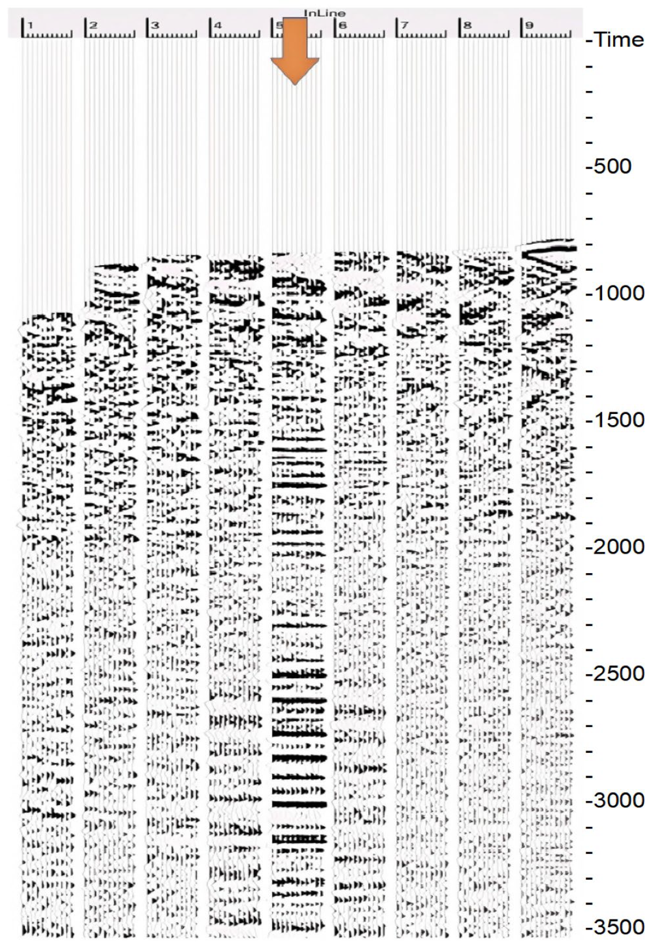
- We formulate velocity spectrum picking under strong multiples as a two-stage detection-and-refinement problem and propose the FLD-PA workflow.
- (2)
- We develop an attention-enhanced YOLOv4-based detector with a CSPBottleneck-Dilated backbone and GIoU loss to improve small-pick localization on velocity spectra.
- (3)
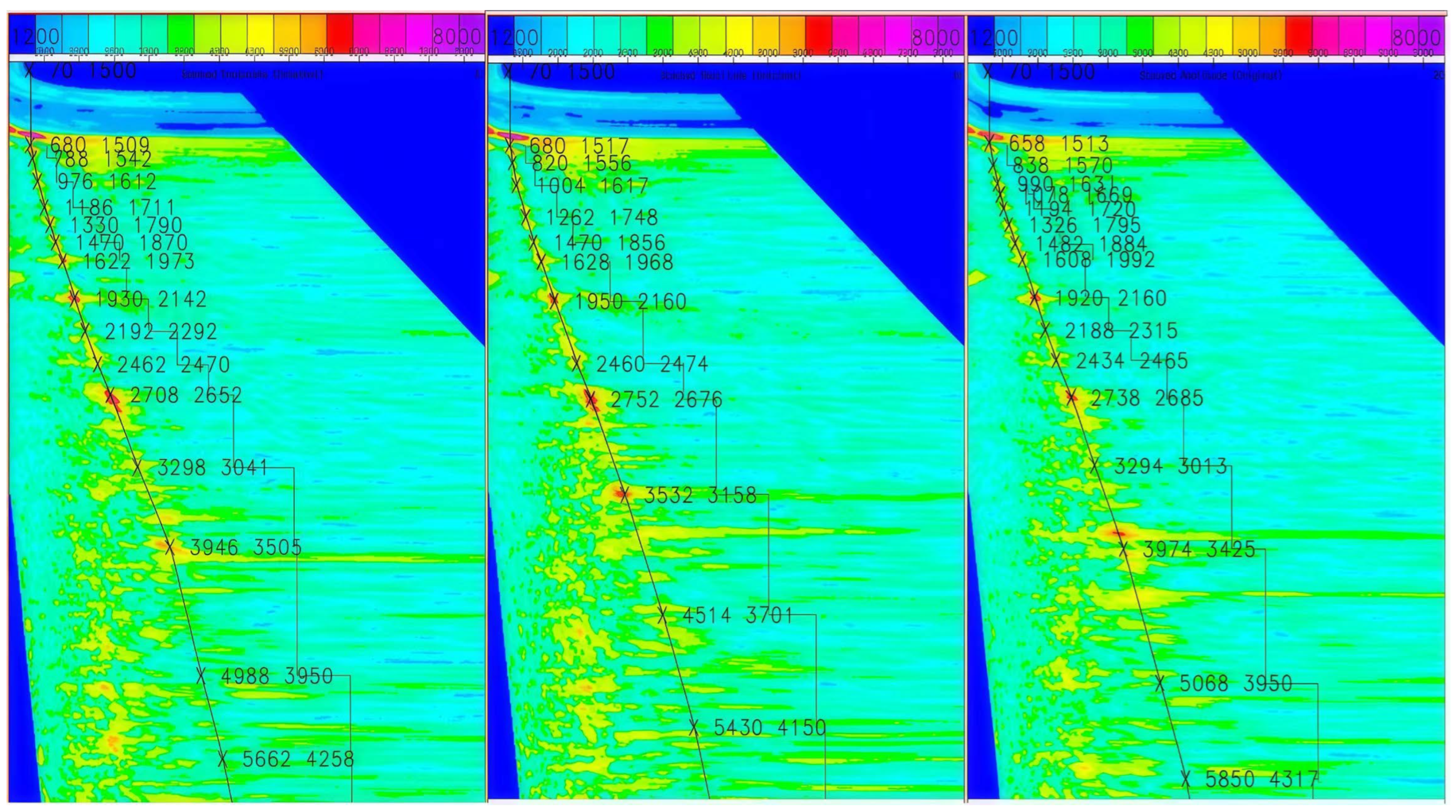
- We introduce a context-constrained PA module that fuses adjacent-spectrum continuity and stacked section energy evidence to refine off-center and weak-energy picks.
- (4)
- We validate the method on two real datasets with strict non-overlapping splits, provide robustness checks and an ablation study, and discuss sensitivity and runtime considerations.
2. Methodological Principles
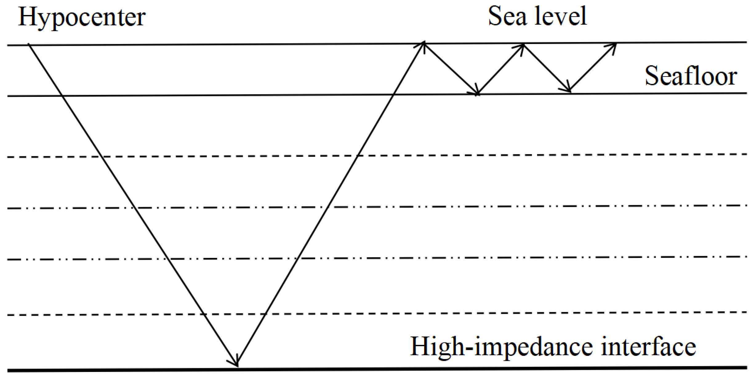
Seismic stacking velocity spectrum picking primarily involves identifying “time-velocity” parameter pairs from high-energy regions within the spectrum’s energy clusters. These parameter pairs are essential for performing normal moveout (NMO) correction and signal stacking on the corresponding common midpoint (CMP) gather [24]. The high-energy region at the center of an energy cluster typically corresponds to an energy extremum; consequently, the velocity at this location often serves as an effective NMO velocity for the CMP gather. Therefore, the NMO correction of seismic data can be framed as a velocity spectrum picking problem. Given that energy clusters contain the necessary features for velocity derivation and that convolutional neural networks (CNNs) excel at image feature extraction, the velocity picking task can be reframed as an image classification and recognition problem. This reframing offers a promising approach for mitigating interference from multiple energy clusters (Figure 1). Furthermore, the picked points from energy clusters exhibit a distinct temporal trend, forming a continuous curve on the velocity spectrum image. This spatial arrangement reflects a contextual dependency along the time axis [25]. These two fundamental characteristics of the velocity spectrum—the energy extrema within clusters and the spatio-temporal correlation of the picking sequence—provide the scientific basis for the subsequent algorithm design.
Figure 1.
Schematic illustration of multiple-reflection generation in submarine environments.
2.1. FLD-PA Overall Model Structure
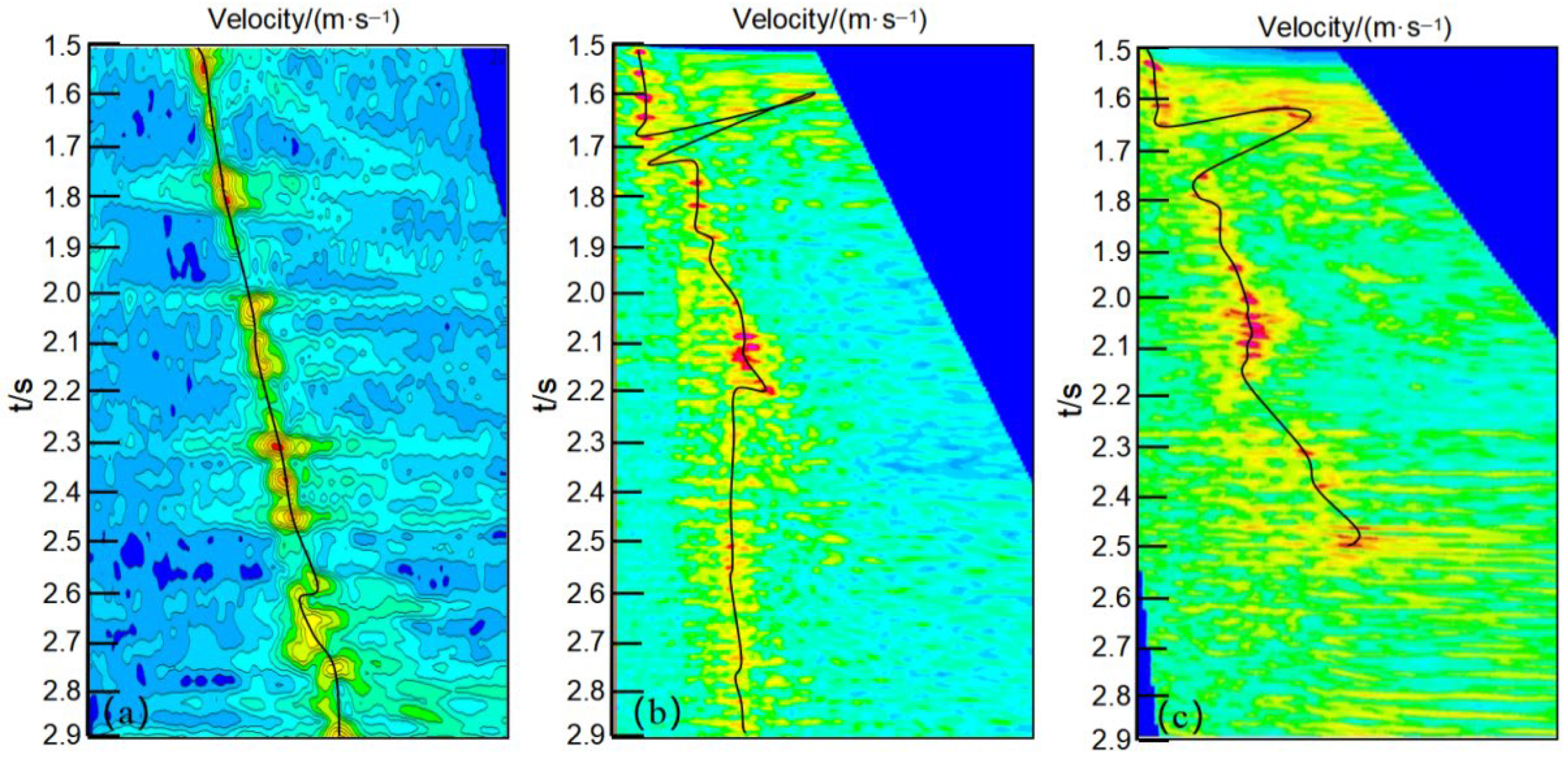
Interference energy clusters, formed by multiple reflections within the velocity spectrum, compromise the accuracy of velocity picking. This inaccuracy, in turn, leads to suboptimal normal moveout (NMO) correction of common midpoint (CMP) gathers and hinders the reliable extraction of velocity parameters. To address this challenge, we focus on regions of the stacking velocity spectrum with a high signal-to-noise ratio, where energy clusters are more regularly distributed. In these regions, we employ the FLD object detection network, based on the YOLO algorithm, as the initial stage of our proposed FLD-PA model. The FLD network is designed to perform an initial coarse picking of high-energy regions within the velocity spectrum. This network leverages an enhanced convolutional neural network module to improve the learning of salient features while suppressing redundant information. This process yields a set of coarse picking points that effectively avoid interference from multiple energy clusters. Finally, these coarse points are connected to establish an initial velocity trend line (Figure 2).
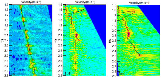
Figure 2.
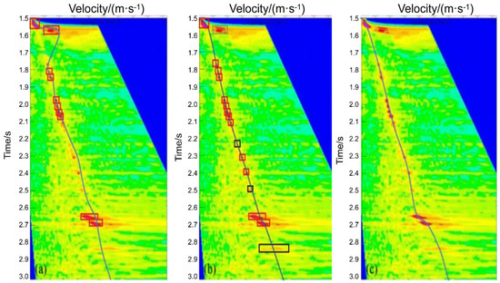
Coarse velocity picks produced by the FLD detector. Panels (a–c) all show the coarse velocity spectrum picking results obtained by the FLD detector.
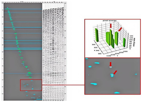
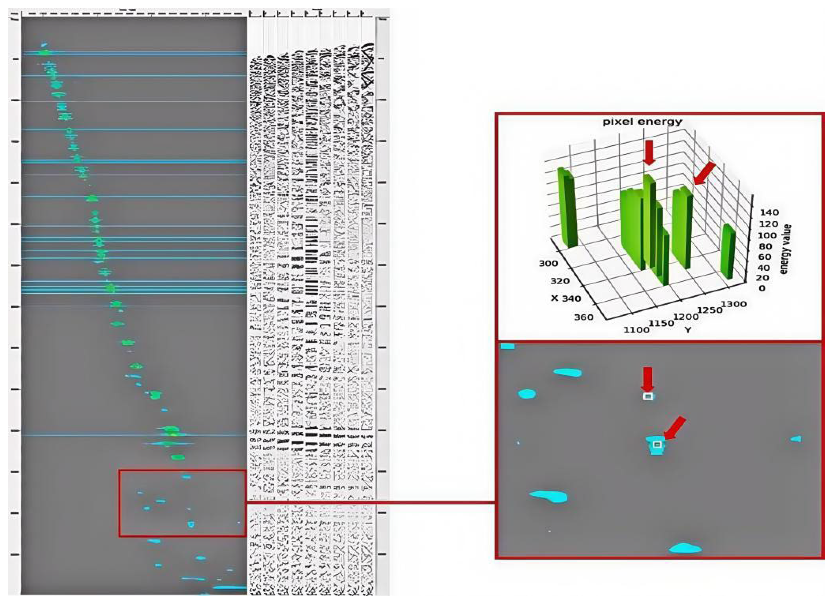
In practice, optimal picking points do not always coincide with energy maxima. Instead, the primary criterion for an accurate pick is the resulting flatness of coherent reflections in the corresponding CMP gather after NMO correction. This discrepancy arises because the semblance distribution can be biased by strong sea-surface-related multiples, limited spectrum resolution, and deviations from the ideal hyperbolic NMO assumption; consequently, a local energy maximum may not correspond to the stacking velocity that best flattens primary events. Furthermore, valid picks may exist in regions with weak or ambiguous energy, while, conversely, picks that deviate from an energy cluster’s center can still be physically meaningful if they improve event flatness and continuity. As shown in Figure 2, the velocity trend line derived from the FLD network’s coarse picks consists largely of points centered on energy clusters, revealing weak sequential correlation. This result contradicts practical scenarios where the optimal picks may deviate from energy centers, especially under strong multiple interference or in weak/ambiguous energy intervals. Such off-center or no-energy picks are difficult to infer from the target spectrum alone because their local contrast is limited and the semblance maximum can be biased. Consequently, always selecting the center of an energy cluster may lead to suboptimal NMO flattening and unreliable velocity parameters.
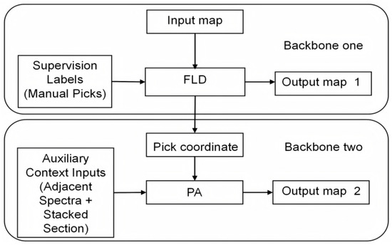
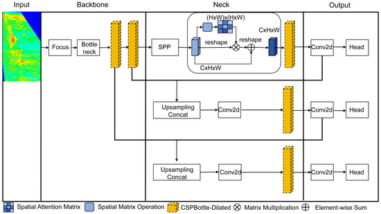
To address this limitation, we introduce a subsequent Point Adjustment (PA) module to refine the coarse picks produced by the FLD network. Rather than arbitrarily moving points, PA constructs a physically constrained correction map by fusing auxiliary seismic context: (i) lateral coherence derived from adjacent velocity spectra, which reflects short-range stratigraphic continuity, and (ii) time consistency evidence from the stacked section, which provides an energy density reference for validating candidate pick times. This correction map narrows the search space to geophysically plausible regions and enables context-aware refinement of pick locations, producing a velocity trend that is more consistent with practical velocity analysis criteria (e.g., improved event coherence/flatness after NMO) and the manual reference labels. The overall two-stage workflow and the role of auxiliary context in PA are summarized in Figure 3.
Figure 3.
Overall architecture of the proposed FLD-PA framework.
As summarized in Figure 3, the proposed FLD-PA framework combines coarse pick localization (FLD) and context-constrained refinement (PA) in a sequential workflow. The key elements include the input velocity spectrum, coarse pick coordinates (box centers predicted by FLD), manual pick labels used for supervision, auxiliary seismic context (adjacent velocity spectra and the paired stacked section), and the outputs before and after refinement.
During training, FLD is supervised using manually picked labels represented by small bounding boxes on velocity spectra. The PA stage does not rely on a separate “second” label set; instead, it uses the same manual pick supervision while taking auxiliary context as additional inputs to construct a correction (energy score) map. Specifically, adjacent velocity spectra provide lateral coherence constraints, and the stacked section provides time consistency evidence for validating/refining the pick time coordinate. In the operational workflow, FLD produces the initial pick sequence (Output Map 1), and PA refines these picks within physically plausible regions defined by the correction map, yielding the final refined results (Output Map 2).
2.2. FLD Model Results of Overall Design
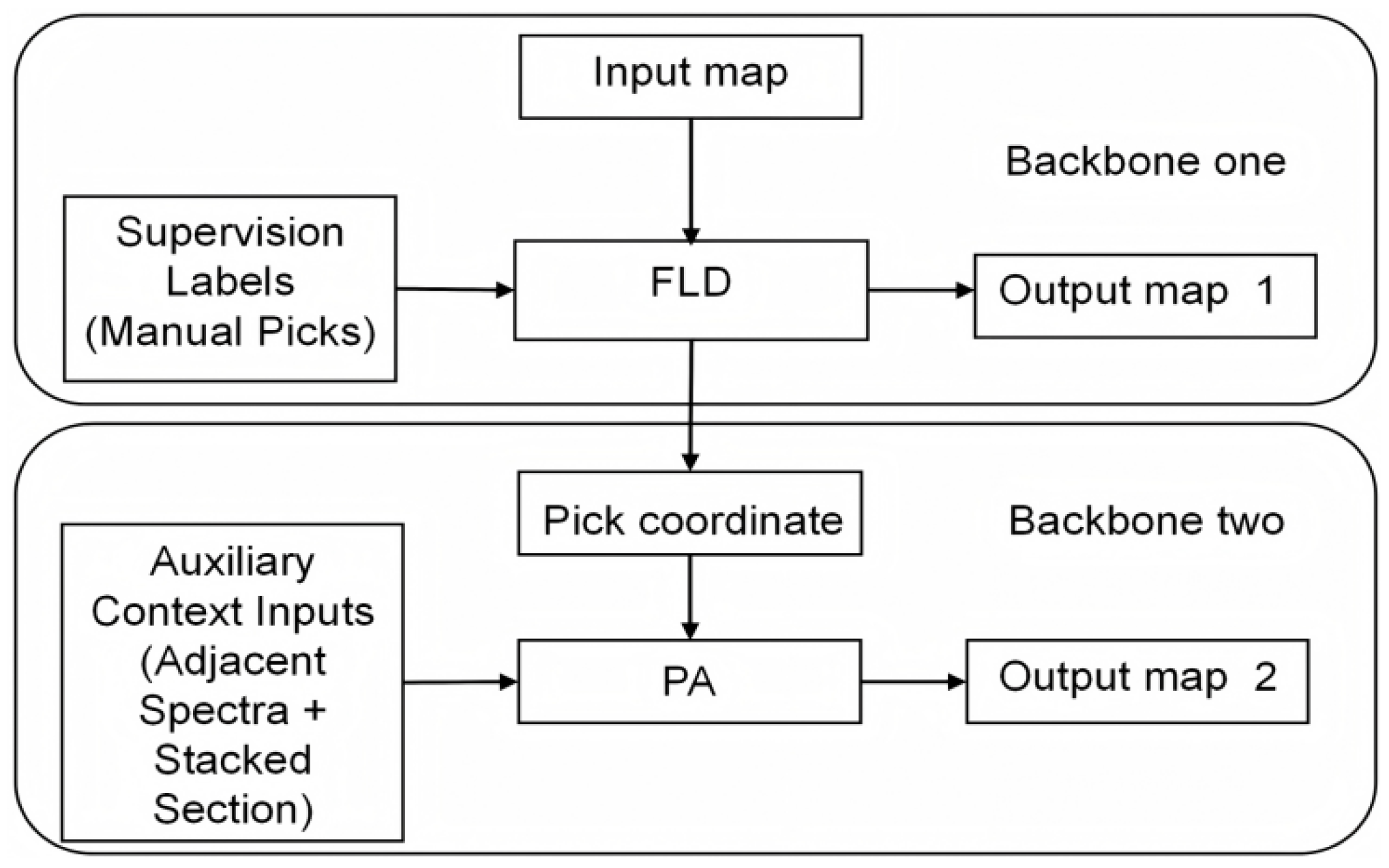
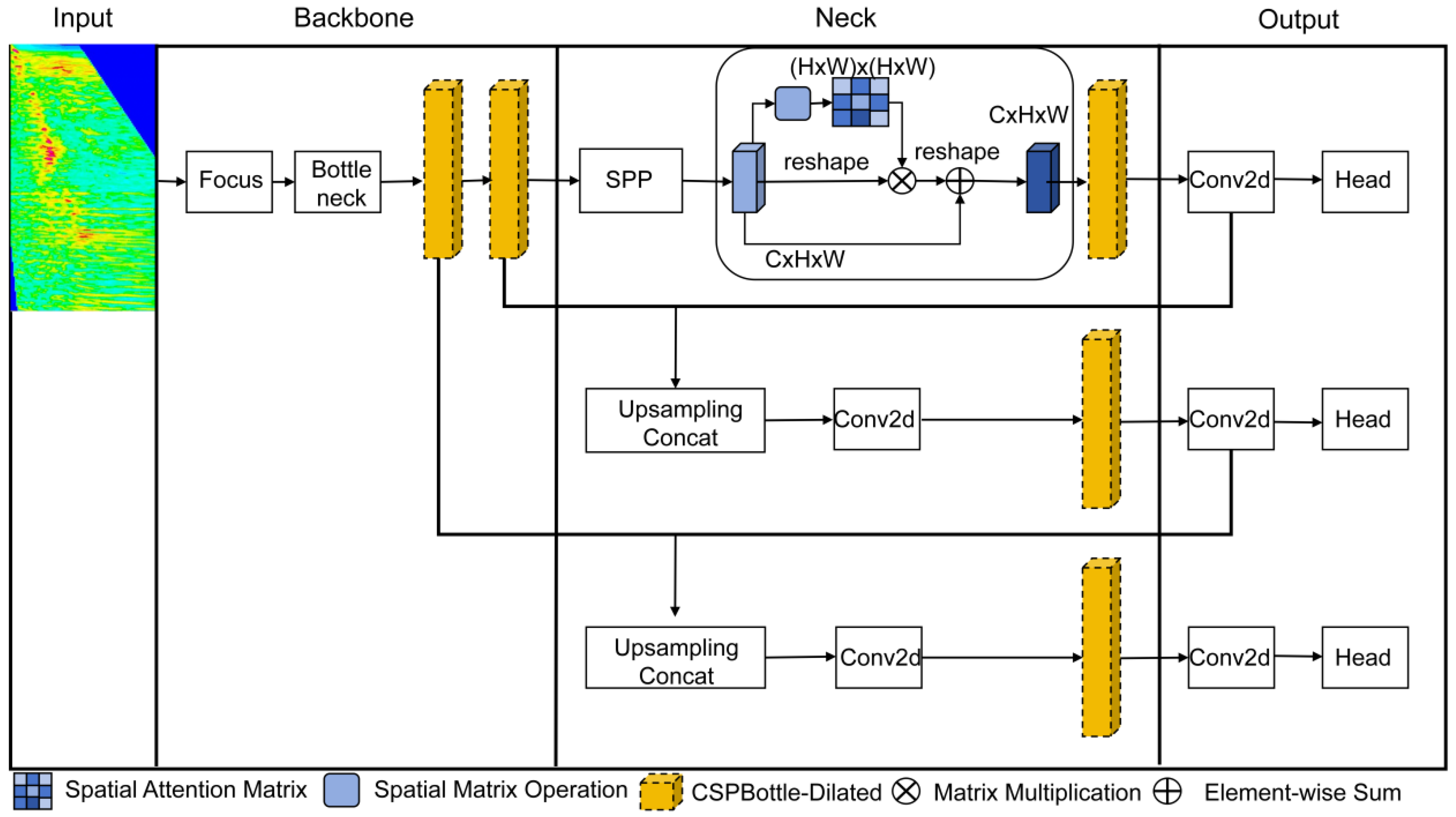
We formulate the first stage of velocity spectrum picking as key-pick localization on the spectrum image. Compared with semantic segmentation, an object-detection formulation is more robust in weak- or no-energy regions and aligns with the practical labeling process, where interpreters provide sparse key picks with small tolerance windows. Accordingly, we adopt a YOLOv4-based detector as the feature-level decoupling (FLD) module (Figure 4). Standard YOLO components are used as in the original implementation, and we focus on three practical modifications for this task: (i) a CSPBottleneck-Dilated block to strengthen multi-scale context, (ii) a lightweight spatial attention module to suppress redundant background, and (iii) GIoU loss for stable training on small (7 × 7-pixel) pick windows [26,27,28,29].
Figure 4.
Overall architecture of the FLD network.
To improve training stability and detection performance under strong multiple interference, we modify three components of the baseline YOLO architecture: the CSPBottleneck block, the spatial attention module, and the box-regression loss.
2.2.1. CSPBottleneck Module
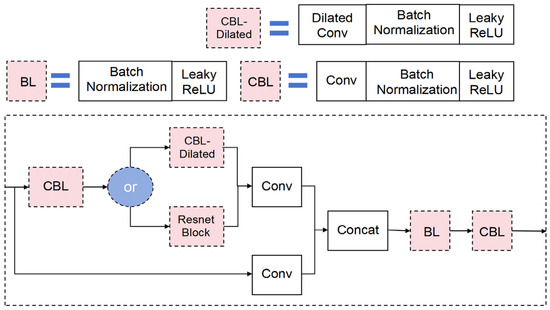
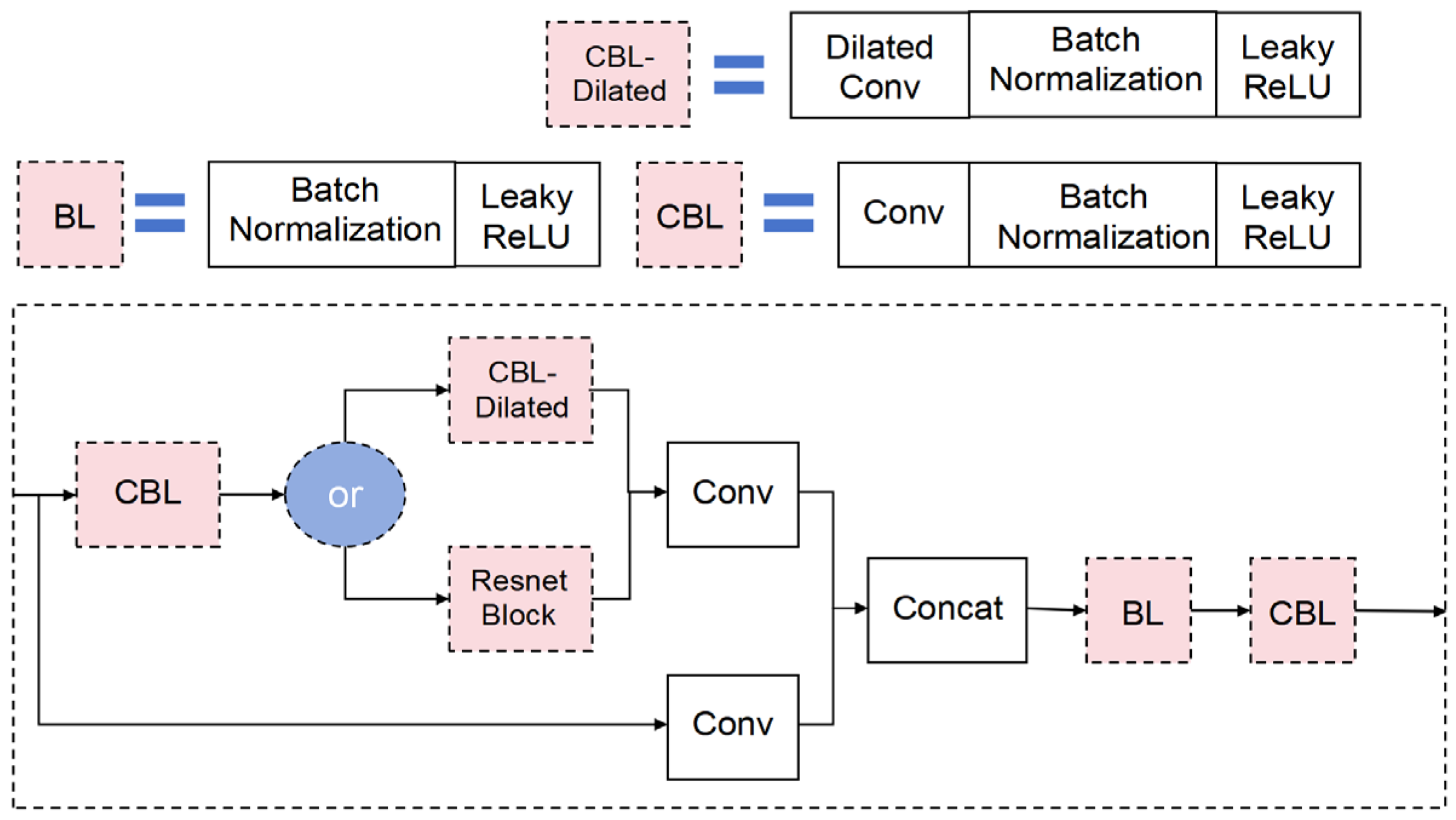
CSPBottleneck-Dilated (Figure 5) replaces the standard bottleneck convolutions with dilated convolutions to enlarge the receptive field without reducing resolution, which helps capture the broader energy-cluster context and improves small-pick localization under strong multiples. We keep the remaining CSP design consistent with the baseline and use Leaky ReLU for stable feature learning on highly similar spectrum textures [30,31,32,33,34].
Figure 5.
CSPBottleneck-Dilated module and the positions of dilated convolutions.
2.2.2. Spatial Attention Module
We insert a lightweight spatial attention (SA) module in the neck to reweight feature maps and suppress low-information background regions (e.g., no-energy areas away from the trend), improving robustness to multiple-related clutter while keeping the detector efficient [35].
2.2.3. Loss Function
We use the Generalized Intersection over Union (GIoU) Loss [36] as the box-regression objective of the FLD detector (Equation (1)). In our dataset, each labeled pick is represented by a small fixed bounding box (7 × 7 pixels) centered on the manually interpreted picking point, so that the detector learns a localized neighborhood of the pick rather than an extended object boundary. During early training, predicted boxes frequently do not overlap with the ground-truth boxes; under the conventional IoU loss, this yields a zero gradient and can stall optimization. GIoU adds a penalty term defined on the smallest enclosing box of the prediction and target, providing informative gradients even when the boxes are disjointed and stabilizing training on small targets.
In Equation (1), IoU denotes the intersection over union between the predicted and ground-truth boxes, U is the union area, and C is the area of the smallest enclosing box covering both. By jointly maximizing IoU while minimizing the enclosing area, GIoU encourages accurate localization of the box center and extent, which is critical for small-label learning. Compared with IoU-only regression, the enclosing box term explicitly measures localization error and mitigates vanishing gradients in the non-overlap regime, leading to more reliable convergence for densely distributed, small targets in velocity spectrum images.
It should be noted that velocity picking is ultimately a continuous-curve estimation problem. We use bounding boxes only as an intermediate representation to exploit the robustness of modern object detectors in the presence of multiple-related interference and in low-energy (no-clear-maximum) regions. The final picking curve is not obtained by the detector alone: we convert the detected boxes into coarse pick coordinates (box centers) and then refine them using the subsequent PA module, which integrates contextual information from adjacent velocity spectra and stacked sections to enforce stratigraphic continuity and geological plausibility. In Section 3, we further evaluate the predicted trend line using curve-level similarity and localization-error metrics (e.g., cosine similarity, Fréchet distance, and RMSE), which better reflect the practical objective of accurate velocity trend recovery.
2.3. FLD Subsequent Processing Flow of Coarsely Picked Network Points
The FLD module first detects a set of small bounding boxes that represent local neighborhoods of candidate picks. We then convert each box to a coarse pick coordinate using its center point and connect these coordinates along the time/depth axis to form an initial velocity trend line. Because a detector is naturally biased toward prominent energy maxima, these coarse picks tend to lie near the centers of energy clusters, which may be suboptimal in the presence of multiple interference or when the optimal NMO-consistent pick is off center. As illustrated in Figure 6, off-center or no-energy picks are difficult to recover from the spectrum image alone because their local texture/energy contrast can be weak or absent. Therefore, the FLD output is treated as a robust, multiple-suppressed initialization rather than the final picking result. To obtain physically plausible and geologically consistent picks, we feed the coarse coordinates into the subsequent Point Adjustment (PA) module, which constrains the valid search region using adjacent-spectrum continuity and stacked section energy evidence, and then refines the pick locations within this constrained region.
Figure 6.
Representative mis-pick patterns in velocity spectra (off-center and no-energy cases).
2.4. Point Adjustment (PA) Algorithm for Fine-Grained Velocity Spectrum Picking
The FLD detector is first applied to generate coarse pick candidates on the velocity spectrum image. With the spatial-attention-enhanced backbone, FLD suppresses a large portion of multiple-related clutter and produces an initial pick sequence that is close to the true velocity trend. However, due to the detector’s preference for prominent local maxima, these coarse picks are often centered on energy clusters, whereas practical velocity analysis may require off-center or weak-energy picks to achieve the best NMO-consistent flattening of primary reflections.
Geophysically, an off-center pick may occur when the semblance maximum is biased by strong multiple interference, limited spectrum resolution, or deviations from the ideal hyperbolic NMO assumption (e.g., non-hyperbolic moveout or anisotropy). In such cases, blindly selecting the energy maximum risks picking multiple-related energy or a biased maximum, which can degrade gather flatness after NMO and introduce systematic velocity errors. Therefore, we introduce a Point Adjustment (PA) algorithm to refine the coarse picks using physically motivated constraints: (i) lateral continuity inferred from adjacent velocity spectra, and (ii) time consistency evidence from the stacked section. Specifically, PA maps adjacent-spectra energy into a constrained search region on the target spectrum and then uses stacked section energy density features to validate and correct the pick time coordinate. This design aims to favor geologically plausible primary-event picks rather than shifting points arbitrarily or following multiple artifacts.
2.4.1. Adjacent Velocity Spectrum Characteristics and Mapping Algorithm
Velocity spectra from neighboring CMP traces exhibit strong similarity because the underlying reflectors are laterally continuous over short offsets and the acquisition/processing conditions are comparable. As a result, the primary reflections that control the correct stacking-velocity trend tend to occur at similar time coordinates across adjacent traces. This lateral coherence provides a physically grounded constraint: if multiple adjacent spectra support a similar pick time, that pick is more likely to correspond to a primary-event velocity trend than to an isolated multiple-related maximum.
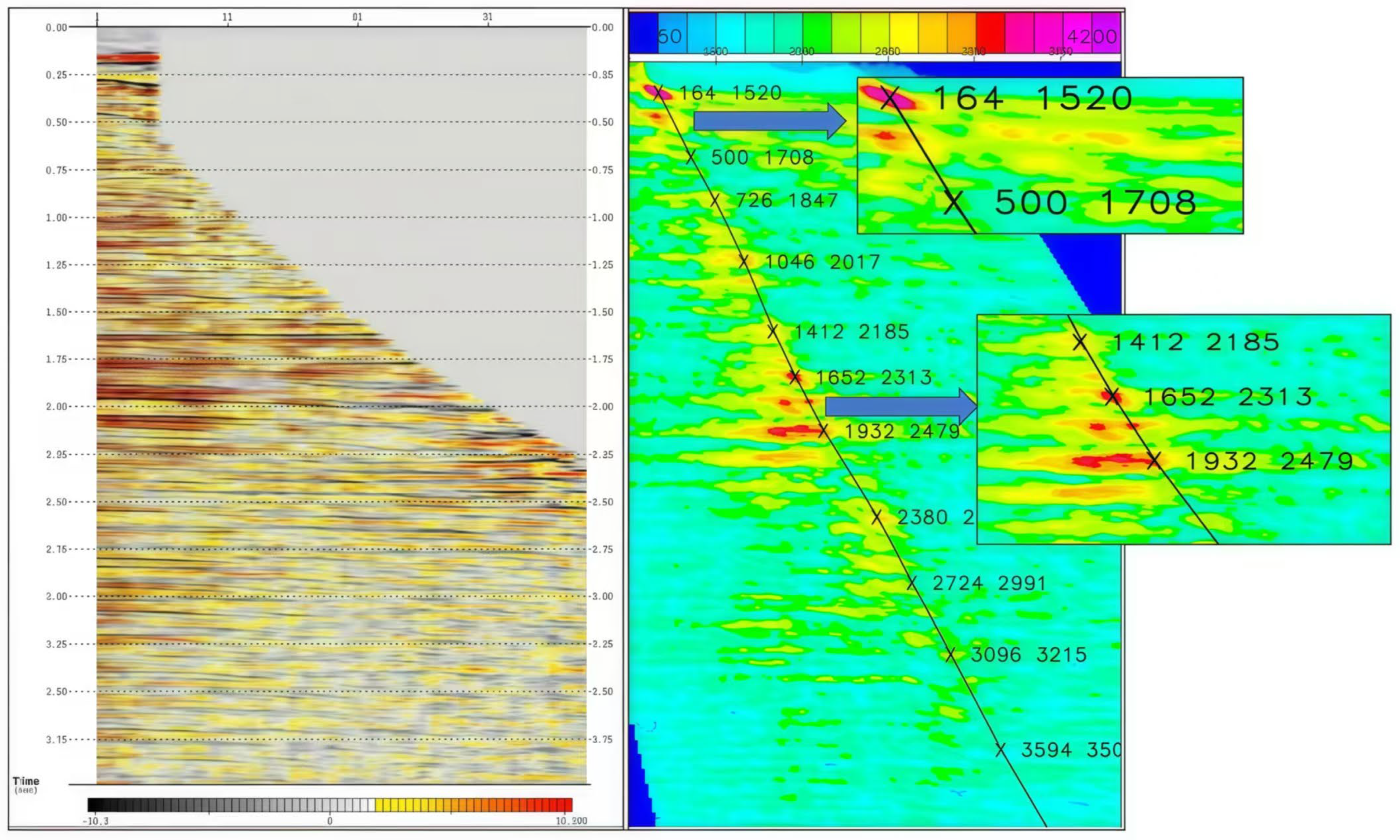
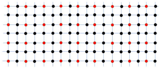
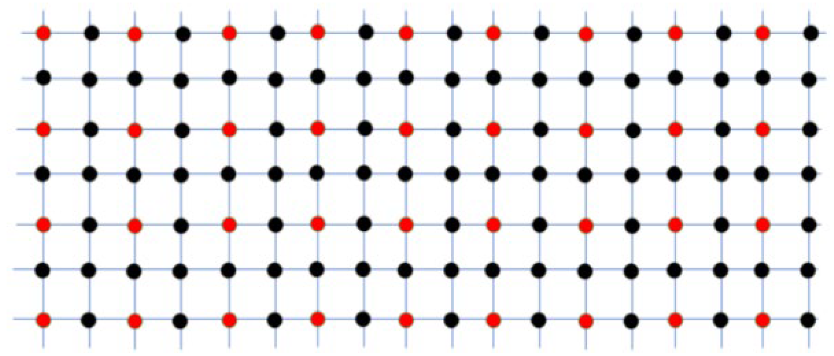
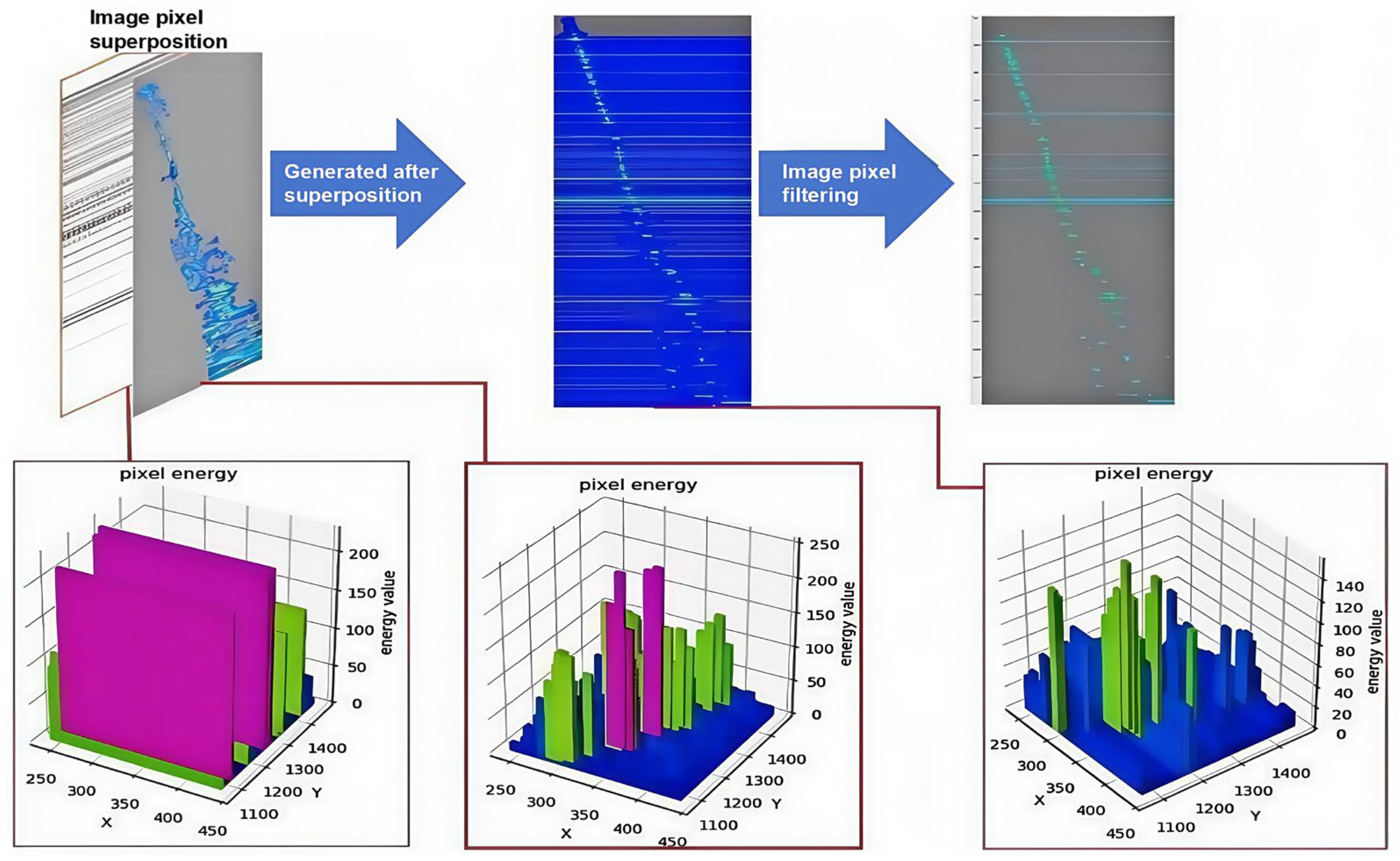
Based on this principle, we define an adjacent-spectra sampling array (Figure 7 and Figure 8) and map the two neighboring spectra (separated by a fixed trace interval) onto the central target spectrum. The goal is to construct an energy-guided search region on the target spectrum that is consistent with adjacent picks. We first convert the spectrum image into an energy matrix using its chrominance components (YUV), and then apply a controlled attenuation to the original target energy to reduce the dominance of both primary and multiple clusters. Next, for each adjacent pick, Rp, we project a circular region of influence, Dp, onto the target spectrum and superimpose a radiated energy field that decays with distance from the Rp, as defined in Equation (2). This mapping boosts the energy intensity around laterally coherent candidate locations while suppressing unrelated clutter, thereby reducing the probability of selecting multiple artifacts.
Figure 7.
Example of the adjacent-spectrum sampling array.
Figure 8.
Example of pick-point correspondence across adjacent velocity spectra.
Our adjacent velocity spectrum mapping algorithm maps two neighboring spectra (separated by three traces) onto a central target spectrum (Figure 8). The algorithm defines a search space on the target spectrum using mapped locations from adjacent picks. It then assigns a score to each candidate point based on its proximity to both the mapped adjacent pick and the local energy center. The process involves three steps: (1) halving the pixel energy of the target spectrum; (2) projecting a circular region of influence from adjacent picks onto it (Figure 9); and (3) superimposing a radiated energy field that decreases outwards from the projected center, as described by Equation (2).
Figure 9.
Schematic of the adjacent-spectrum energy mapping algorithm.
In Equation (2), E(n,m) denotes the energy at pixel coordinate (n,m), Rp is the mapped coordinate of an adjacent pick, and Dp is the circular radiation zone around Rp. The resulting mapped energy E′(n,m) is accumulated into the final adjacent-energy matrix P (Equation (3)), where α is a scaling coefficient (typically 0.5) controlling the attenuation strength.
The adjacent-spectrum mapping procedure is described above and implemented consistently for all spectra in the PA module.
By analyzing the mapping relationship between adjacent picks, potential picking locations on the target spectrum can be determined even when the target spectrum exhibits weak or ambiguous energy. The attenuation factor α reduces the overall energy of multiple and primary clusters, while the mapping process selectively enhances the laterally consistent region, making valid candidate picks stand out relative to multiple-dominated regions. Finally, a coarse trend derived from the FLD picks is intersected with the mapped adjacent-spectra trend, and the optimal candidate is selected by searching for the maximum energy within the radiated region along this intersection.
2.4.2. Overlay Segment Characteristics and Mapping Algorithm
The stacked section provides an additional seismic-context constraint for validating the pick time coordinate (vertical axis). Because the stacked section aggregates CMP energy across a scanned velocity range, coherent primary reflections tend to manifest as high-energy-density bands, which can serve as evidence for whether a candidate pick time is geologically plausible. Therefore, a physically consistent pick should be supported not only by spectrum energy and lateral coherence from adjacent spectra, but also by an energy density peak in the stacked section at the corresponding time neighborhood.
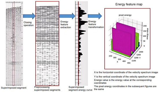
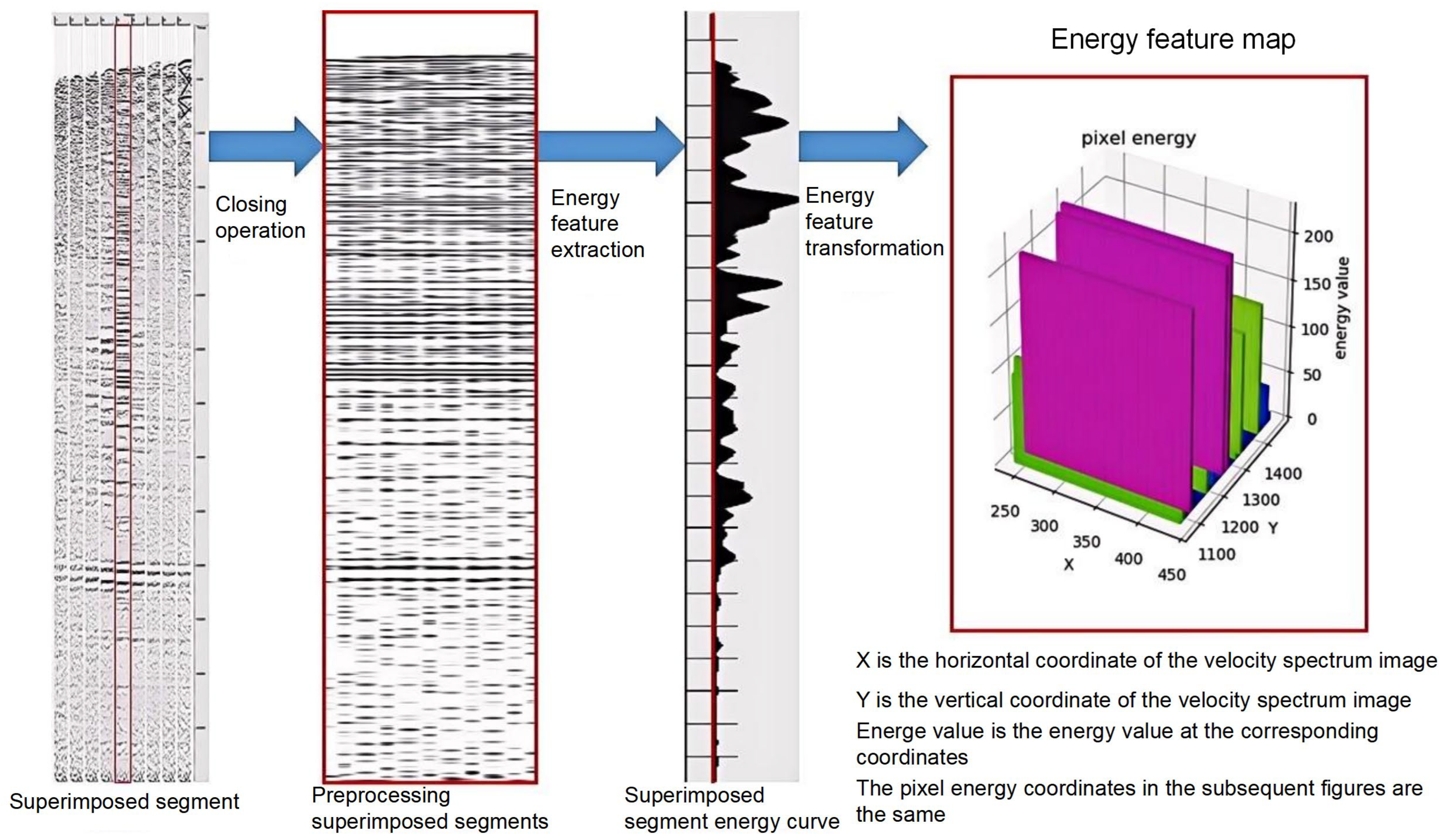
To extract robust energy evidence, we apply a morphological closing operation (2 × 2 kernel) to the stacked section image to suppress small discontinuities and noise. We then compute an energy density curve along time and convert it into a matrix representation for subsequent fusion. This stacked section energy feature acts as a reference that helps correct time/depth deviations and prevents error accumulation along the time axis. Importantly, the stacked section is used as a validation and correction cue rather than a standalone decision rule, since residual multiples may still influence stacked energy; the final picks are determined under the joint constraints of adjacent-spectrum continuity and stacked section evidence.
Following the stacked section processing, its energy map is integrated with the initial map (derived from adjacent spectra) via an additional weighted summation. This step yields the final weighted energy matrix P. This transformation is expressed as Equation (4), a modification of Equation (3).
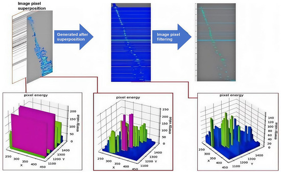
Here, β is a variable coefficient (typically 0.5), and C(n,m) is the energy value at coordinate (n, m) in the stacked section’s energy feature matrix (Figure 10 and Figure 11). Applying this transformation pixel-wise yields the optimal energy score map, P′, as illustrated in Figure 12. This optimal score map, P′, which consolidates the fused features, is defined in Equation (5).
Figure 10.
Superposition segment model.
Figure 11.
Overlay segment processing flow (the red box and red line indicate the selected overlay segment).
Figure 12.
Energy fusion process for generating the optimal energy score map.
Finally, we perform a cross-picking operation between P′ and the coarse FLD picks to restrict candidates to physically plausible intersection zones and apply non-maximum suppression to refine picks within the mapped regions. This step both improves localization robustness in weak energy intervals and filters redundant picks, producing the final refined results shown in Figure 13.
Figure 13.
Final refined picks on the optimal energy score map.
3. Model Validation and Analysis
First, we compare the coarse picks from FLD against representative detection baselines. We then quantify trend similarity using curve-level metrics (e.g., cosine similarity and Fréchet distance) in addition to pick-level errors. Next, we benchmark the complete FLD–PA workflow against two learning-based picking baselines (YOLOv8-LSTM and a CNN transfer-learning approach). Finally, we provide qualitative comparisons to illustrate behavior under different multiple-interference patterns.
3.1. Dataset Preparation and Evaluation Metrics
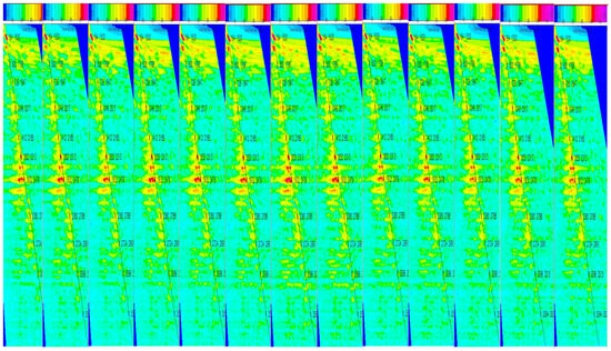
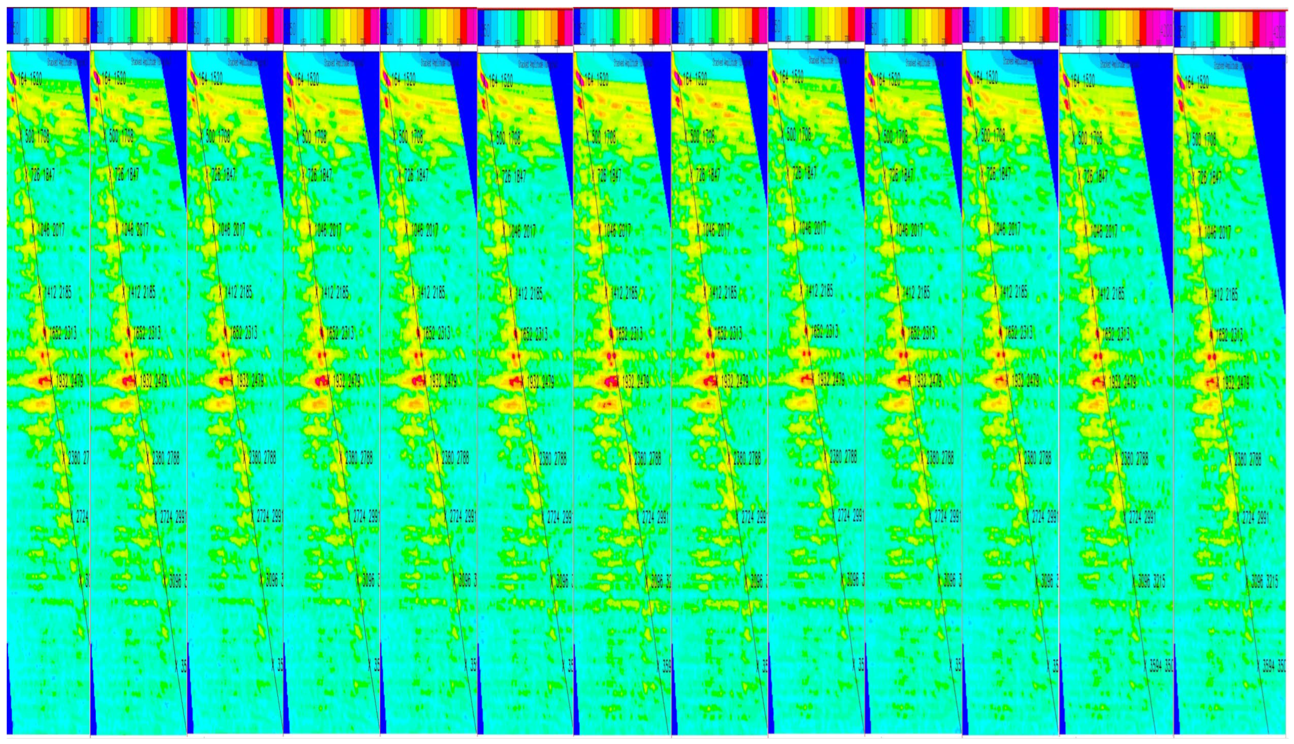
The dataset, extracted using GeoEast V4.4 software, comprises velocity spectra and their corresponding stacked sections from a single survey area. Spectra were sampled using the previously described trace-skipping interval, with ground-truth picks manually annotated. Each velocity spectrum is paired with a corresponding stacked section, enabling their use as mutual references (Figure 14).
Figure 14.
Examples of adjacent velocity spectrum images used in PA.
We validate the proposed method on two real seismic datasets derived from the same offshore survey area (the same acquisition campaign) but sampled from non-overlapping CMP/line subsets to ensure a strict hold-out evaluation. Dataset 1 contains velocity spectra with moderate-to-strong multiples and is used for training/validation and in-domain testing. Dataset 2 is a fully held-out subset from the same survey area with systematically stronger multiple interference and different acquisition/processing conditions (e.g., different sail lines, different CMP ranges, and/or different stacking velocities), and is used to stress test generalization within the same field. This design avoids data leakage while controlling for geological setting, which makes the comparison of primary/multiple discrimination and picking robustness more meaningful.
The current validation has some limitations. The two datasets were extracted from a single survey campaign; therefore, the reported results primarily demonstrate robustness across heterogeneous subsets within this project (e.g., across CMP ranges and local variability) rather than full cross-survey generalization. Due to data availability and confidentiality constraints, we cannot include an independent external survey in this revision. To partially mitigate this limitation, we (i) perform within-survey cross-validation by rotating the train/validation split, and (ii) conduct stress tests on challenging spectra with strong multiples, weak deep events, and ambiguous/no-energy intervals to evaluate whether the method consistently recovers physically plausible trends under varying SNR and interference conditions. Future work will validate the approach on additional surveys with different geology and acquisition/processing workflows.
To meet processing requirements, we established a unified dimensional standard for the dataset. Velocity spectra and their corresponding stacked sections were extracted to ensure a consistent scale along the time axis. Annotations were made as precisely as possible using 7 × 7 pixel bounding boxes. These annotations were then used to generate a dataset in the PASCAL VOC standard format. The chrominance (YUV) components of the images, treated as energy values, were converted into a matrix format for input to the PA module.
The reference trend lines were produced by experienced velocity analysts using GeoEast V4.4 velocity analysis. Following a standardized protocol applied consistently across the dataset, analysts tracked the primary-energy ridge from shallow to deep time while using the corresponding stacked section as an auxiliary cue for event continuity and rejecting obvious multiple-related ridges. A subsequent QC pass was checked for unrealistic velocity jumps and for poor event flattening after NMO, and the picks were corrected when needed. The finalized pick coordinates were converted into fixed 7 × 7-pixel boxes centered at each pick for detector training and evaluation.
Network detection accuracy was evaluated using precision and recall, as defined in Equations (6) and (7), respectively.
In this context, true positives (TPs) are correctly identified picks, false negatives (FNs) are valid picks that the model failed to identify, and false positives (FPs) are incorrect picks identified by the model.
Picking error and pick-level metrics. Let (x_i, y_i) be the predicted pick center and (x_i*, y_i*) the reference pick center on the velocity spectrum image. We define the per-pick localization error e_i, the root mean square error (RMSE), and the tolerance-based picking accuracy PA(τ) as follows (τ = 10 pixels in this work):
In our application, the physically relevant error is the velocity–axis deviation. Because the time coordinate is constrained by the sampling grid and the PA refinement, Equation (8) mainly reflects velocity–axis misalignment; in practice, we also report velocity–axis RMSE by projecting the error onto the velocity axis when required.
In all experiments, we set τ = 10 pixels, approximately the diagonal of the 7 × 7 manual pick window, so that a prediction falling within the annotated neighborhood is counted as acceptable. Pixel offsets can be converted to physical velocity errors (m/s) using the velocity–axis scaling of the spectrum image:
3.2. Experimental Procedures and Setup
Our experimental workflow proceeds in five stages:
- Architectural validation of the FLD detector by benchmarking against mainstream object detectors under the same detection-stage protocol.
- Within-survey robustness evaluation of FLD via cross-validation by rotating the training/validation split.
- Baseline comparison against representative velocity-picking networks implemented in this study under the same detection-stage evaluation protocol.
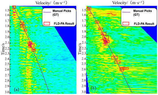
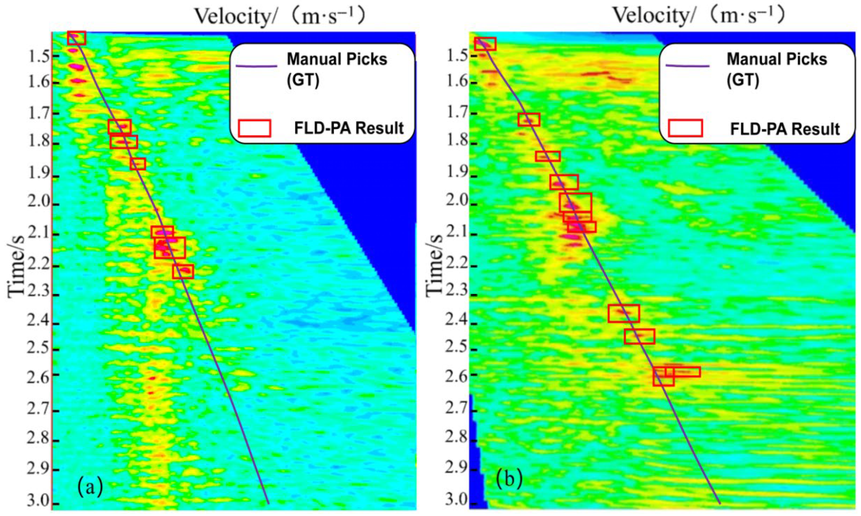
- Analysis of metric suitability: we examine why IoU-based precision/recall can be overly strict for small pick windows and support this with qualitative visualization (Figure 15) and curve-level trend-similarity metrics.Figure 15. Detection results on (a) Dataset 1 and (b) Dataset 2. The purple curve indicates the manual pick (ground truth), and the red boxes mark the detected pick windows (FLD–PA).
- Final picking-quality evaluation using pick-level metrics (RMSE and PA), including both the default operating point and a matched-recall setting for a fair comparison with YOLOv8–LSTM). RMSE is reported in pixel units on the velocity spectrum image for consistency with the annotated pick windows, and pixel offsets can be converted to velocity error (m/s) using the velocity–axis scaling of the spectrum image.
3.2.1. FLD Module Experiment
In this experiment, we benchmarked our proposed FLD network against several prominent object detection architectures. All models were trained for 100 epochs with a batch size of 4. The results, presented in Table 1, show that our proposed FLD network achieved the highest picking performance among the tested architectures. This superior performance is attributed to the combination of its CSP structure, dilated convolutions, and spatial attention mechanism, which collectively enhance feature learning within the picking regions. Despite the prevalence of off-center picks in the dataset, the attention mechanism robustly learns relevant features from these challenging regions.
In Table 1, val-precision is computed on the validation split, while test precision and test recall are computed on the held-out test split under the same IoU criterion. We also report the F1 score, defined as F1 = 2PR/(P + R), where P and R denote test precision and test recall, respectively. Although some detectors achieve relatively high recall, FLD yields the best overall F1, indicating a more favorable precision–recall trade-off for small (7 × 7-pixel) pick windows.
Table 1.
Comparison of mainstream detectors in terms of detection-stage performance (test set precision, recall, and F1).
To assess robustness within the considered survey dataset, we employ cross-validation by rotating the training/validation split. This evaluation focuses on within-survey robustness rather than cross-survey generalization, consistent with the limitation stated in Section 2.1. The results of this analysis are presented in Table 2.
Table 2.
Within-survey robustness of FLD using cross-validation.
The results from this 300-epoch experiment (batch size of 3) indicate that the FLD network is robust against overfitting, suggesting it effectively learned the textural features of the energy clusters during training.
Next, we benchmarked the FLD algorithm against other established velocity-picking methods. While the CNN and YOLOv8 models were trained with a batch size of 8, our FLD network used a batch size of 3; all models were trained for 300 epochs. The comparative results are shown in Table 3.
Table 3.
Comparison of representative baseline implementations under the same detection-stage evaluation protocol (test set precision, recall, and F1). F1 is computed from test precision and recall.
Baseline selection and scope. We compare FLD–PA primarily against two representative learning-based velocity-picking baselines implemented under the same data splits and evaluation protocol: (i) a YOLOv8–LSTM pipeline that couples detector outputs with sequence modeling, and (ii) a CNN transfer-learning method that predicts a continuous velocity trend. In addition, to provide a representative segmentation-based comparison, we include a U-Net ridge-extraction baseline. Because our confidential labeling workflow provides sparse pick points rather than dense masks, we generate thin-band segmentation labels by connecting the manual picks into a curve and dilating it by a small fixed width. We acknowledge that broader coverage of segmentation/regression paradigms and validation on independent surveys would further strengthen the assessment, and we leave such extensions to future work, where the F1 score is computed as:
Across all detector-stage experiments (Table 1, Table 2 and Table 3), IoU-based precision scores remain below 50% (e.g., 34.11% for FLD), which could be misinterpreted as poor performance if viewed in isolation. This is mainly due to the discrete-threshold behavior of IoU on very small targets (7 × 7 pixels): minor center shifts can flip matches across the IoU threshold and inflate FP/FN counts. Importantly, curve-level visualization and similarity metrics show that the predicted trends still align closely with the manual trend (Figure 15 and Table 4). For practical velocity analysis, the decisive quantity is the resulting trend consistency and pick localization error; therefore, Table 5 and Table 6 report RMSE and PA as pick-level metrics that directly reflect the usability of the picked stacking-velocity trend under multiple interference.
As shown in Figure 15, the FLD network effectively suppresses interference from multiples. The resulting velocity trend line is qualitatively strong, with most picks located on or near the manually interpreted ground truth. Therefore, to quantitatively assess the similarity between the predicted and ground-truth trend lines, we employ two metrics: average cosine similarity and the Fréchet distance [39].
The results in Table 4 are based on two metrics. Cosine similarity quantifies the similarity between two vectors by measuring the cosine of the angle between them; a value approaching 1 indicates high similarity. By extension, the average cosine similarity quantifies the overall similarity between two curves. The Fréchet distance is a measure of spatial similarity between curves, where a smaller value indicates a higher degree of similarity.
For two velocity curves resampled at the same N time samples, let v_pred and v_gt denote the corresponding velocity vectors (in pixel units along the velocity axis). The cosine similarity is defined as:
We compute the discrete Fréchet distance between two 2D polylines P = (p1, …, pN) and Q = (q1, …, qN) in the image coordinate system, where pi = (ti, v_pred,i) and qi = (ti, v_gt,i). Let d(pi,qj) = ||pi-qj||2. The discrete Fréchet distance is defined by:
To remove dependence on axis scaling, we additionally report a normalized distance FD_norm computed after axis-wise min-max normalization of time and velocity to [0,1]:
Table 4.
Quantitative evaluation of velocity trend similarity (CosSim, FD_px (px), and FD_norm).
In our evaluation, a cosine similarity approaching 1 and small Fréchet distances indicate high trend-line similarity between the predicted and manual velocity curves. Notably, these curve-level metrics can remain high even when IoU-based precision/recall are low for small pick windows, supporting the conclusion that curve-level and pick-level metrics are more informative for assessing practical picking quality in this task.
The performance discrepancy across different metrics highlights three key characteristics of our dataset: (1) a high prevalence of off-center picks; (2) numerous valid picks in no-energy regions; and (3) small annotation bounding boxes. These factors explain why conventional deep learning networks alone are insufficient to achieve optimal results on this dataset. While smaller bounding boxes reduce localization error, they are heavily penalized by IoU-based metrics. Even minor misalignments can lead to a low intersection over union, which in turn lowers the measured precision. Conversely, enlarging the bounding boxes would artificially inflate IoU and precision scores without improving the actual localization accuracy of the pick’s center point.
Accordingly, we evaluate the final picks using localization-error metrics (RMSE) and tolerance-based picking accuracy PA as defined in Section 3.1.
3.2.2. FLD-PA Experiment
We evaluate the final picking accuracy using RMSE and PA, which quantify point-wise deviation between predicted picks and manual picks. Table 5 summarizes the results on the training and testing datasets. RMSE is reported in pixel units on the velocity spectrum image, and PA represents the percentage of picked samples whose errors fall within a predefined tolerance (see Section 3.1 for the explicit definition). These picking-level metrics directly reflect practical accuracy and complement the detection-stage metrics reported in Table 1, Table 2 and Table 3.
In response to the reviewer’s concern about modest numerical gains, we additionally report multi-seed variability for FLD–PA and a per-scenario paired analysis on representative challenging spectra (Appendix A.3). The gains remain consistent across random seeds and across these scenarios, supporting the robustness of the reported improvements.
To further ensure a fair comparison with YOLOv8–LSTM, we report a matched-recall comparison (≈81%) by selecting detector confidence thresholds on a held-out validation subset (Appendix A.2). Table 6 reports the selected thresholds and shows that, at controlled recall, FLD–PA yields lower RMSE and higher PA@10px, indicating more consistent trend refinement in difficult spectra containing strong multiple interference.
Table 5.
Picking performance comparison (RMSE and PA) of different methods on the training and testing datasets. RMSE is reported in pixel units on the velocity spectrum image.
Table 6.
Picking performance comparison under a matched-recall setting (recall ≈ 81%). The selected confidence thresholds and the achieved validation recall are reported for reproducibility. RMSE is reported in pixel units on the velocity spectrum image.
Matched-recall evaluation. Because confidence threshold choices can change the number of returned picks and the detector recall, we additionally report a matched-recall comparison between FLD–PA and the strongest baseline (YOLOv8–LSTM). We tune the detector confidence threshold for each of these two methods on a held-out validation subset to match a target recall of ≈81% (computed using the same IoU criterion as in the main text) and then evaluate RMSE and PA@10px on the test subset at the selected operating points. Appendix A.2 provides the exact protocol and the FLD threshold sweep used for operating-point selection.
The YOLOv8-LSTM algorithm, an automated method combining YOLOv8 output with a long short-term memory (LSTM) network, excels at learning sequential features, giving it a significant advantage in picking accuracy. The model effectively captures the contextual features of energy cluster picks by feeding confidence scores, bounding box dimensions, and center-point coordinates from YOLOv8 into an LSTM for sequential learning. However, a major limitation is its fixed-count output. This constraint is a significant source of error on real-world data, where the true number of valid picks is variable. This fixed-count approach artificially inflates the RMSE and reduces the PA score, thereby compromising overall picking accuracy. Furthermore, the algorithm is prone to erroneously picking multiple energy clusters, which further degrades its RMSE and PA scores. In contrast, our FLD-PA method leverages an attention mechanism to capture multi-level information and suppress interference from multiples. Critically, it does not impose a fixed-count output. By deriving sequential features from adjacent spectra, our algorithm produces more geologically plausible and realistic results.
The CNN-Transfer method classifies velocity spectrum patches to determine NMO velocity. These classified patches are used to train a CNN, which is then fine-tuned for other datasets using transfer learning. Because this algorithm only outputs a continuous velocity trend line without identifying discrete picks, a PA metric comparison is impossible. However, its high RMSE value reveals suboptimal performance, with large velocity deviations in complex geological areas. In comparison, our FLD-PA method achieves a superior RMSE, indicating that its results more closely align with the ground truth and are better suited for real-world picking challenges. By dynamically adjusting the pick count, our FLD-PA algorithm flexibly adapts to the complexities of different geological settings.
3.2.3. Comparison of Experimental Results
To further validate robustness under challenging conditions within a single survey campaign, we select velocity spectra containing complex energy clusters (including strong multiple interference and weak deep events) and compare different picking strategies. This analysis emphasizes difficult within-project cases and is designed to complement the held-out evaluation on Dataset 2 and the cross-validation results.
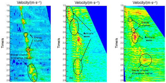
We selected several representative spectra with complex energy-cluster patterns (e.g., strong multiple interference, crossing events, and weak deep primaries) for qualitative evaluation. These challenging cases were manually annotated and are shown in Figure 16.
Figure 16.
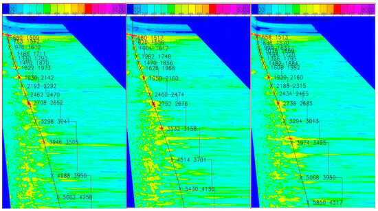
Different types of energy clusters. (a) Velocity spectrum with complex energy clusters in the mid-to-deep section. (b) Velocity spectrum with significant multiple energy clusters. (c) Velocity spectrum from a complex geological structure, showing prominent multiples.
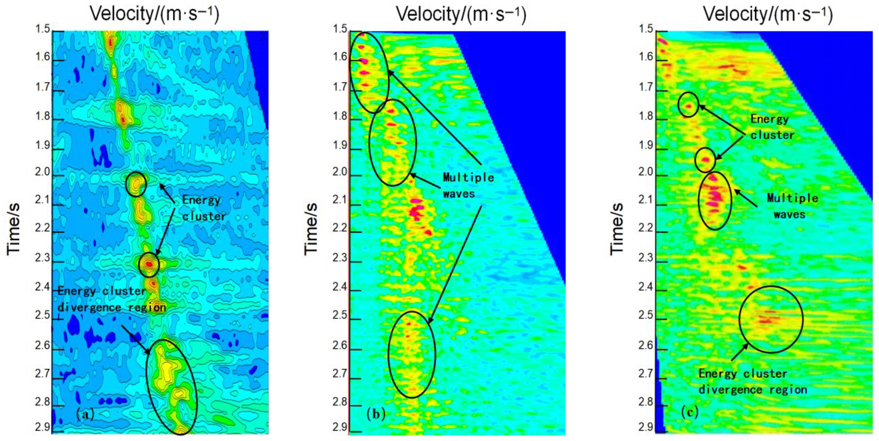
Multiples, a typical form of coherent noise, arise from repeated reflections of a seismic wave between a near-surface low-velocity layer and a deeper reflector, and they typically appear as repetitive, regular waveforms. This interference can produce spatial aliasing, leading to two primary issues: the crossing of coherent reflections with primary waves, and the introduction of spurious energy clusters during velocity analysis. Both of these effects compromise the accuracy and reliability of the resulting velocity spectrum.
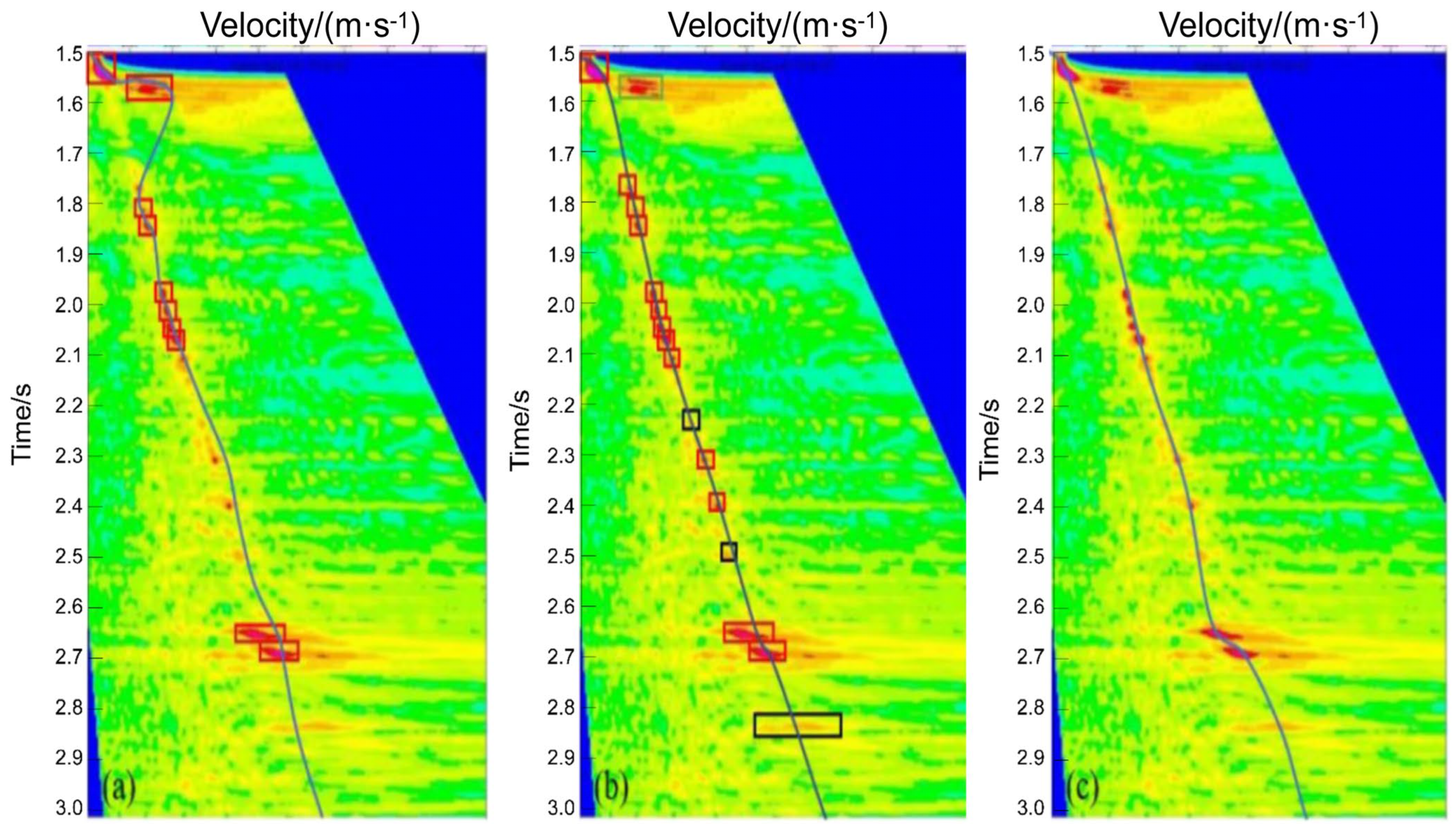
To validate the advantages of our proposed FLD-PA model, we performed picking on the challenging velocity spectra from Figure 16 using three different methods: (1) our FLD-PA model, (2) a conventional CNN+RNN fusion model, and (3) manual interpretation (ground truth). The resulting picks from each method were connected to form trend lines for a comparative analysis, as shown in Figure 17.
Figure 17.
Comparison of three velocity spectrum picking methods. (a) Conventional CNN+RNN. (b) FLD-PA model. (c) Manual picking (ground truth).
While conventional CNNs effectively identify shallow-to-mid depth energy clusters, they struggle with weaker, deeper ones. We therefore fed the CNN-derived coordinates into an RNN to predict the locations of these faint, deep clusters. The final results were then compared against manual picks and our FLD-PA model’s output to comprehensively evaluate the performance of all three methods.
As shown in Figure 17, the three picking methods exhibit distinct behaviors. Panel (a) shows the results from the conventional CNN+RNN model. Because the CNN is less reliable on mid-to-deep energy clusters, gaps appear in the predicted sequence, which limits the RNN’s ability to learn a stable trend and leads to larger errors.
Panel (b) displays the results from our proposed FLD-PA model, where the red squares represent the initial coarse picks from the FLD network. Compared with the manual ground truth in Panel (c), minor deviations remain in a few complex, wide energy clusters, which we attribute to the detector’s sensitivity to local maxima and cluster width. In these cases, the refinement stage may occasionally over-adjust, and additional cross-survey validation will be explored to further strengthen the robustness of the refinement process.
Nevertheless, the results in Table 5 indicate that both the FLD module’s initial picks and the PA module’s subsequent refinements are highly accurate. The complete FLD-PA algorithm meets automation requirements, exhibits strong multiple suppression, and successfully identifies valid off-center picks.
3.2.4. Failure Modes and Efficiency Considerations
Although FLD–PA is effective at suppressing multiple-related clutter, its response can be less efficient in a few challenging situations. First, when energy clusters are extremely wide, merged, or exhibit multiple comparable local maxima, the detector may lock onto a suboptimal extremum, leading to small but noticeable offsets. Second, the PA stage leverages short-range lateral continuity; abrupt lateral velocity changes (e.g., faults or rapid stratigraphic variations) can weaken this assumption and may cause over-smoothing or occasional over-adjustment. Third, the stacked section cue used for time consistency may be contaminated by residual multiples or imaging artifacts, which can bias the correction map in limited intervals. From a computational perspective, FLD inference is a single forward pass, while PA refinement is lightweight and scales approximately linearly with the number of spectra and samples; it can be parallelized across spectra and accelerated by restricting the refinement window to high-confidence regions. These considerations explain the minor deviations observed in a few complex spectra and motivate future extensions such as adaptive constraint weighting, uncertainty-aware refinement, and broader cross-survey validation.
3.2.5. Additional Experiments: Ablation, Operating-Point Analysis, and Runtime Considerations
To strengthen validation, we include an ablation study that isolates the contribution of each component in the proposed FLD–PA workflow. We additionally provide operating-point sensitivity, multi-seed variability, a per-scenario breakdown (Appendix A.2 and Appendix A.3), and runtime measurements for practical deployment. All analyses use the same train/test splits described in Section 3.1 and the same evaluation protocol and metrics defined in Section 3.2.
In our ablation study, we compare four variants: (a) a baseline detector followed by a conventional curve fitting step (without feature-level decoupling), (b) FLD only (detector output converted to picks using the same curve fitting step), (c) FLD + PA without the physics constraint term, and (d) the full FLD–PA workflow. By keeping the data, splits, and post-processing consistent, this study verifies that the observed improvements are attributable to the proposed design (FLD and PA, as well as the physics constraint), rather than a single tuning choice.
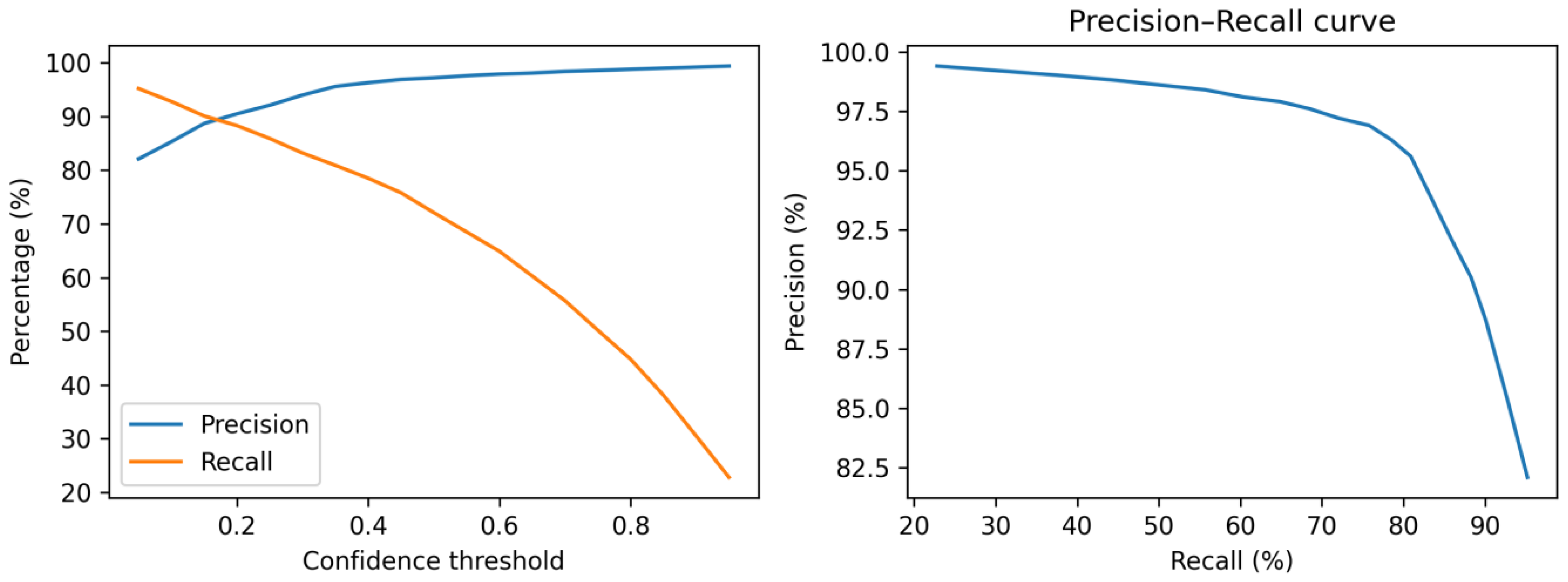
For sensitivity analysis, to quantify operating-point robustness, we sweep the detector confidence threshold from 0.05 to 0.95 and report the resulting precision/recall trade-off (Table A1) and curves (Figure A1) in Appendix A.2. This analysis also supports the matched-recall setting used for fair comparison with YOLOv8–LSTM (Table 6). In addition, we report multi-seed variability (Table A2) and a per-scenario breakdown (Table A3) in Appendix A.3.
For runtime analysis, we measure the end-to-end inference time per velocity spectrum on the Dataset 1 test set using an NVIDIA Tesla V100 GPU for FLD inference and an Intel Xeon Gold 6248 CPU for PA refinement (10 repeated runs, reporting mean ± standard deviation). Table 7 reports the per-spectrum runtime of each stage and the full workflow (serial and parallel). Table 8 further reports the total runtime versus the number of spectra to illustrate scalability and practical throughput for large-scale 3D surveys.
In this work, mAP@0.5 is computed on the detector outputs by treating each labeled picking region as an instance and using an IoU threshold of 0.5, while RMSE/MAE are computed on the final picking curves after post-processing.
Together, these additional experiments provide evidence of effectiveness (Table 9) and robustness across operating points (Table 5 and Table 6), and they clarify practical runtime considerations for deployment.
Table 7.
Measured runtime of the FLD–PA workflow on the Dataset 1 test set.
Table 8.
Scalability analysis of total runtime versus the number of spectra.
Table 9.
Ablation study of the proposed FLD–PA workflow.
Together, these additional experiments provide evidence of effectiveness (Table 8), robustness (Appendix A.2 and Appendix A.3), and efficiency (Table 8 and Table 9), addressing the request for more comprehensive validation.
4. Conclusions
This paper proposes the FLD-PA workflow to address two practical failure modes in automatic velocity spectrum picking under strong multiples: (i) mis-picks caused by multiple-related clutter and (ii) off-center/no-energy picks caused by weak events and sparse labels. The workflow integrates a robust detector (FLD) and a context-aware refinement module (PA):
- Robust first-stage detector (FLD): To reduce mis-picks caused by multiple-related energy clusters, we adapt a YOLOv4-style detector for key-pick localization on velocity spectra and incorporate task-oriented improvements (CSPBottleneck-Dilated and spatial attention) together with GIoU loss for stable training on small (7 × 7-pixel) pick windows. On the detector-stage benchmark, FLD improves test precision from 14.58% (YOLOv8) to 34.11% (+19.53 percentage points) and achieves the best overall F1 among the compared detectors.
- Physics-informed contextual refinement (PA): To correct off-center and no-energy picks, we propose a refinement module that fuses adjacent-spectrum lateral continuity and stacked section time consistency evidence to constrain a feasible search region and adjust coarse picks toward a geophysically plausible velocity trend. This refinement improves stability in weak energy intervals and reduces the influence of multiple-related clutter.
On the held-out test set, FLD-PA improves picking accuracy (PA@10px) from 91.50% to 93.14% (+1.64 percentage points) and reduces RMSE from 12.4 px to 10.15 px (−2.25 px) compared with YOLOv8-LSTM. Under a matched-recall setting (≈81%), the comparison is performed at validation-selected operating points with the same recall (Table 6 and Appendix A.2), and FLD-PA remains more accurate (higher PA@10px and lower RMSE) than YOLOv8-LSTM. The recovered velocity trend is highly consistent with manual interpretation (cosine similarity > 0.99 and Fréchet distance < 50 px).
Overall, FLD-PA improves the robustness of velocity spectrum picking under strong multiple interference by combining detection-based localization with physics-informed contextual refinement. The method reduces multiple-induced mis-picks and yields more consistent stacking-velocity trends on the tested datasets, particularly in off-center and weak energy scenarios. However, the current validation is limited to subsets extracted from a single survey campaign; therefore, the results primarily demonstrate intra-survey robustness rather than full cross-survey generalization. Future work will include external cross-survey evaluation and NMO-consistency-based quantitative validation to further establish the physical interpretability and generalization of the refinement process.
Author Contributions
Conceptualization, S.Z. and X.Z.; methodology, S.Z.; software, X.Z.; validation, X.Z. and S.C.; formal analysis, X.Z.; investigation, X.Z. and S.C.; resources, S.Z.; data curation, S.Z.; writing—original draft preparation, X.Z.; writing—review and editing, S.Z.; visualization, X.Z.; supervision, F.C.; project administration, S.Z.; funding acquisition, S.Z. All authors have read and agreed to the published version of the manuscript.
Funding
This work was supported by the Henan Province Science and Technology Research Project (Grant No. 252102210222).
Institutional Review Board Statement
Not applicable.
Informed Consent Statement
Not applicable.
Data Availability Statement
The data used in this study are not publicly available due to confidentiality restrictions. Derived data and/or trained model outputs that support the findings of this study are available from the corresponding author upon reasonable request, subject to approval from the data owner. To support reproducibility despite data confidentiality, we provide detailed evaluation definitions and an implementation summary (including PA pseudocode and key training/evaluation settings) in Appendix A, and the training scripts/configuration files can be shared upon reasonable request subject to institutional approval.
Acknowledgments
The authors thank the data provider for permission to use the seismic data in this study.
Conflicts of Interest
The authors declare no conflicts of interest.
Appendix A. Reproducibility and Implementation Details
This appendix summarizes key implementation details to facilitate replication of the proposed workflow when data access is available. Unless otherwise stated, all experiments use the dataset splits described in Section 3.1 and the evaluation protocol in Section 3.2.
Appendix A.1. Key Training and Evaluation Settings
- Input: velocity spectrum images paired with stacked section images; pick labels represented by fixed 7 × 7-pixel boxes centered at manual picks (Section 3.1).
- Detector evaluation: mAP@0.5 and precision/recall use an IoU threshold of 0.5 (Section 3.1 and Section 3.2.5).
- Picking-level evaluation: RMSE and PA computed on pick centers with τ = 10 pixels (Section 3.1).
- Matched-recall evaluation: we tune the detector confidence threshold on a held-out validation subset to match the target recall (≈81%) for FLD–PA and YOLOv8–LSTM, and then report PA@10px/RMSE at that operating point on the test subset (see Appendix A.2 for details).
Appendix A.2. Matched-Recall Operating-Point Selection and Sensitivity Analysis
We define a matched-recall operating point as follows. Because the detector confidence threshold monotonically controls the number of returned pick windows, we use it as the operating parameter for both FLD and YOLOv8–LSTM. On a held-out validation subset, we perform a grid search over candidate thresholds {0.05, 0.10, …, 0.95}. For each threshold, we compute precision and recall using the same IoU criterion as in the main text. We select the threshold whose recall is closest to the target (81%); if multiple thresholds tie, we choose the one with higher precision. The selected threshold is fixed and used for evaluation on the test subset. In our experiments, the operating point closest to 81% recall is obtained at threshold = 0.35 for FLD (recall = 80.9%), and at threshold = 0.50 for YOLOv8–LSTM (recall = 81.0%). Table A1 reports the FLD sweep, and Figure A1 visualizes the corresponding precision–recall trade-off.
Table A1.
Threshold sweep for FLD on the validation subset (IoU = 0.5). Precision/recall are in %.
Figure A1.
Sensitivity of FLD to the confidence threshold: precision/recall curves (left) and the precision–recall curve (right).
Appendix A.3. Statistical Support for Performance Gains
To quantify variability, we repeated FLD–PA training and evaluation with three random seeds. The results are stable: PA@10px = 93.03 ± 0.15% (mean ± std) and RMSE = 10.20 ± 0.10 px (Table A2). To provide a scenario-level breakdown, Table A3 reports five representative challenging spectra (grouped by energy-cluster types) and compares FLD–PA with the YOLOv8–LSTM baseline. In these cases, FLD–PA reduces RMSE by 4.12 px on average (95% bootstrap CI: [3.34, 4.66] px). A paired t-test indicates the RMSE reduction is significant on this subset (p < 0.001), while we caution that this table is intended as an illustrative per-scenario analysis rather than a full test set re-evaluation.
Table A2.
Multi-seed variability of FLD–PA on the test subset (mean and standard deviation are summarized in the text).
Table A3.
Per-scenario comparison on representative challenging spectra (PA@10px is binary for each single-spectrum case: 1 if the pick error e_i ≤ 10 px, otherwise 0). Scenarios are grouped by typical energy-cluster/interference patterns observed in the test subset.
Appendix A.4. PA Refinement Pseudocode (High-Level)
| Algorithm A1: PA refinement (high-level) |
| Input: target spectrum S_k; adjacent spectra {S_{k-m}, …, S_{k + m}}; stacked section G_k; coarse picks P = {(x_i, y_i)}; parameters (m, D_p, β). Output: refined picks P′. 1: E_adj <- AdjacentSpectrumMap(S_k, {S_{k-m}…S_{k + m}}, P, D_p) # Section 2.4.1 2: E_stack <- StackedSectionMap(G_k) # Section 2.4.2 3: M <- Normalize(E_adj) + β * Normalize(E_stack) 4: for each (x_i, y_i) in P do 5: (x_i′, y_i′) <- argmax_{(x,y) ∈ W(x_i, y_i)} M(x, y) 6: end for 7: return P′ = {(x_i′, y_i′)} |
References
- Pan, H.X.; Sun, K.F.; Ye, Y. New advances in seismic velocity analysis techniques. Prog. Explor. Geophys. 2008, 31, 172–177. [Google Scholar]
- Meng, F.K. Research on an Automatic Picking Algorithm of Seismic Stacking Velocity Spectrum Based on Deep Learning. Master’s Thesis, North China University of Water Resources and Electric Power, Zhengzhou, China, 2024. [Google Scholar]
- LeCun, Y.; Bengio, Y.; Hinton, G. Deep learning. Nature 2015, 521, 436–444. [Google Scholar] [CrossRef] [Scilit] [PubMed]
- Wu, X.; Yan, S.; Qi, J.; Zeng, H. Deep learning for characterizing paleokarst collapse features in 3D seismic images. J. Geophys. Res. Solid Earth 2020, 125, e2020JB019685. [Google Scholar] [CrossRef] [Scilit]
- Dong, L.P.; He, X. Automatic picking of velocity spectra using artificial neural networks. Oil Geophys. Prospect. 1996, S1, 98–103. [Google Scholar] [CrossRef]
- Wang, L.X. Automatic picking of stacking velocity and a method for extracting migration velocity. Geophys. Prospect. Pet. 1999, 38, 107–113. [Google Scholar]
- Zhang, J.H.; Wang, J.; Zheng, X.G.; Shan, L.Y.; Xu, H.; Fu, J.R.; Yu, H.C.; Bu, C.C. Discussion and performance analysis of several velocity analysis methods. Geophys. Prospect. Pet. 2009, 48, 347–353. [Google Scholar] [CrossRef]
- David, E.L. Monte Carlo automatic velocity picks. Stanf. Explor. Proj. Rep. 1997, 75, 1–25. [Google Scholar]
- Toldi, L.T. Velocity analysis without picking. J. Geophys. 1989, 54, 191–199. [Google Scholar] [CrossRef] [Scilit]
- Lin, N.T.; Liu, H.; Li, G.H.; Tang, J.J.; Wei, L.J. Path-integral optimization and smoothing techniques for automatic velocity picking. Chin. J. Geophys. 2013, 56, 246–254. [Google Scholar]
- Zhang, J.B.; Lin, N.T.; Zhang, D.; Zhao, C.W.; Yang, X.C. Intelligent picking of velocity spectra based on nonlinear functions. Prog. Geophys. 2016, 31, 856–860. [Google Scholar] [CrossRef]
- Liu, A.Q.; Tong, C.X.; Li, L. Study on velocity analysis methods and influencing factors in the Yingdong Slope Belt. Prog. Geophys. 2008, 23, 1909–1917. [Google Scholar]
- Fish, B.C.; Kusuma, T. A neural network approach to automate velocity picking. In Expanded Abstracts of the 64th Annual International SEG Meeting; Society of Exploration Geophysicists: Tulsa, OK, USA, 1994; pp. 185–188. [Google Scholar] [CrossRef] [Scilit]
- Pan, H.X.; Geng, W.F.; Cui, J.H.; Bian, C.; Zhao, H.; Zhao, X.R. Deep learning methods for intelligent picking of seismic velocity spectra. Prog. Geophys. 2023, 38, 2553–2564. [Google Scholar]
- Kuang, L.C.; Liu, H.; Ren, Y.L.; Luo, K.; Shi, M.Y.; Su, J.; Li, X. Application status and development trends of artificial intelligence in petroleum exploration and development. Pet. Explor. Dev. 2021, 48, 908. [Google Scholar] [CrossRef] [Scilit]
- Huang, K.Y.; Yang, J.R. Seismic velocity picking using Hopfield neural network. In Proceedings of the SEG International Exposition and 85th Annual Meeting, New Orleans, LA, USA, 18–23 October 2015; Society of Exploration Geophysicists: Tulsa, OK, USA, 2015. [Google Scholar]
- Biswas, R.; Vassiliou, A.; Stromberg, R.; Sen, M.K. Stacking velocity estimation using recurrent neural network. In Proceedings of the SEG Technical Program Expanded Abstracts; Society of Exploration Geophysicists: Tulsa, OK, USA, 2018; pp. 2241–2245. [Google Scholar] [CrossRef] [Scilit]
- Fabien-Ouellet, G.; Sarkar, R. Seismic velocity estimation: A deep recurrent neural-network approach. Geophysics 2020, 85, U21–U29. [Google Scholar] [CrossRef] [Scilit]
- Park, M.J.; Sacchi, M.D. Automatic velocity analysis using convolutional neural network and transfer learning. Geophysics 2020, 85, V33–V43. [Google Scholar] [CrossRef] [Scilit]
- Ma, H.Y. Key Technologies for Velocity Spectrum Picking in Seismic Wavelet Correction. Master’s Thesis, North China University of Technology, Beijing, China, 2021. [Google Scholar] [CrossRef]
- Hochreiter, S.; Schmidhuber, J. Long short-term memory. Neural Comput. 1997, 9, 1735–1780. [Google Scholar] [CrossRef] [Scilit]
- Girshick, R. Fast R-CNN. In Proceedings of the IEEE International Conference on Computer Vision (ICCV), Santiago, Chile, 13–16 December 2015; pp. 1440–1448. [Google Scholar]
- Wang, D.; Yuan, S.Y.; Yuan, H.; Zeng, H.H.; Wang, S.X. Unsupervised clustering-based intelligent velocity picking with adaptive threshold constraints. Chin. J. Geophys. 2021, 64, 1048–1060. [Google Scholar] [CrossRef]
- Wang, R.L.; Feng, B.; Wu, C.L.; Wang, H.Z.; Zhang, M. Study on an initial velocity modeling method based on CMP gather intelligence. Geophys. Prospect. Pet. 2021, 60, 763–772. [Google Scholar] [CrossRef]
- Zhang, H.; Zhu, P.M.; Gu, Y.; Li, X.Z. Automatic picking of seismic velocity spectra based on deep learning. Geophys. Prospect. Pet. 2019, 58, 724–733. [Google Scholar] [CrossRef]
- Redmon, J.; Divvala, S.; Girshick, R.; Farhadi, A. You only look once: Unified, real-time object detection. In Proceedings of the IEEE Conference on Computer Vision and Pattern Recognition (CVPR), Las Vegas, NV, USA, 27–30 June 2016; pp. 779–788. [Google Scholar]
- Liu, W.; Anguelov, D.; Erhan, D.; Szegedy, C.; Reed, S.; Fu, C.-Y.; Berg, A.C. SSD: Single Shot MultiBox Detector. In Computer Vision—ECCV 2016; Springer: Cham, Switzerland, 2016; Volume 9905, pp. 21–37. [Google Scholar]
- Lin, T.Y.; Goyal, P.; Girshick, R.; He, K.; Dollár, P. Focal loss for dense object detection. In Proceedings of the IEEE International Conference on Computer Vision (ICCV), Venice, Italy, 22–29 October 2017; pp. 2980–2988. [Google Scholar]
- He, K.; Gkioxari, G.; Dollár, P.; Girshick, R. Mask R-CNN. In Proceedings of the IEEE International Conference on Computer Vision (ICCV), Venice, Italy, 22–29 October 2017; pp. 2961–2969. [Google Scholar]
- Yu, F.; Koltun, V. Multi-scale context aggregation by dilated convolutions. arXiv 2015, arXiv:1511.07122. [Google Scholar]
- Wang, C.-Y.; Liao, H.-Y.M.; Wu, Y.-H.; Chen, P.-Y.; Hsieh, J.-W.; Yeh, I.-H. CSPNet: A new backbone that can enhance learning capability of CNN. In Proceedings of the IEEE/CVF Conference on Computer Vision and Pattern Recognition (CVPR), Long Beach, CA, USA, 16–20 June 2019. [Google Scholar]
- Nair, V.; Hinton, G.E. Rectified linear units improve restricted Boltzmann machines. In Proceedings of the 27th International Conference on Machine Learning (ICML), Haifa, Israel, 21–24 June 2010. [Google Scholar]
- Ioffe, S.; Szegedy, C. Batch normalization: Accelerating deep network training by reducing internal covariate shift. In Proceedings of the 32nd International Conference on Machine Learning (ICML), Lille, France, 6–11 July 2015; pp. 448–456. [Google Scholar]
- He, K.; Zhang, X.; Ren, S.; Sun, J. Deep residual learning for image recognition. In Proceedings of the IEEE Conference on Computer Vision and Pattern Recognition (CVPR), Las Vegas, NV, USA, 27–30 June 2016; pp. 770–778. [Google Scholar]
- Woo, S.; Park, J.; Lee, J.-Y.; Kweon, I.S. CBAM: Convolutional Block Attention Module. In Proceedings of the European Conference on Computer Vision (ECCV), Munich, Germany, 8–14 September 2018; Springer: Cham, Switzerland, 2018. [Google Scholar]
- Rezatofighi, H.; Tsoi, N.; Gwak, J.Y.; Sadeghian, A.; Reid, I.; Savarese, S. Generalized intersection over union: A metric and a loss for bounding box regression. In Proceedings of the IEEE/CVF Conference on Computer Vision and Pattern Recognition (CVPR), Long Beach, CA, USA, 16–20 June 2019. [Google Scholar]
- Ren, S.; He, K.; Girshick, R.; Sun, J. Faster R-CNN: Towards real-time object detection with region proposal networks. IEEE Trans. Pattern Anal. Mach. Intell. 2017, 39, 1137–1149. [Google Scholar] [CrossRef] [Scilit] [PubMed]
- Redmon, J.; Farhadi, A. YOLOv3: An incremental improvement. arXiv 2018, arXiv:1804.02767. [Google Scholar] [CrossRef] [Scilit]
- Eiter, T.; Mannila, H. Computing the Discrete Fréchet Distance. In Technical Report CD-TR 94/64; Technical University of Vienna: Vienna, Austria, 1994. [Google Scholar]

Disclaimer/Publisher’s Note: The statements, opinions and data contained in all publications are solely those of the individual author(s) and contributor(s) and not of MDPI and/or the editor(s). MDPI and/or the editor(s) disclaim responsibility for any injury to people or property resulting from any ideas, methods, instructions or products referred to in the content. |
© 2026 by the authors. Licensee MDPI, Basel, Switzerland. This article is an open access article distributed under the terms and conditions of the Creative Commons Attribution (CC BY) license.