


Abstract
An integrated nonlinear dynamic model was developed to investigate resonance in a four-cylinder engine mounted on a viscoelastic foundation. A coupled lumped-parameter formulation captures vertical and torsional responses under unbalanced inertial forces, combustion torque, and stochastic base excitation. Time-domain simulations show that at low rotational speeds the vertical displacement reaches transient amplitudes before converging to periodic oscillations, whereas higher excitation speeds reduce steady-state amplitudes. Torsional motion exhibits initial angles near 0.05 rad that decay below 0.01 rad in steady state, with further reduction at higher speeds. Frequency-domain analysis indicates that vibration energy is concentrated in engine-order harmonics between approximately 8 and 50 Hz, while components above 60 Hz are strongly attenuated, yielding a dynamic range exceeding 50 dB. Finite element modal analysis identifies the first four structural modes between 18 Hz and 666 Hz, revealing an increasingly dominant overall translational mode and a localized directional behavior at higher frequencies. A high-dimensional kernel density spectrogram integrates modal and spectral features to map resonance regions. Results indicate that increasing rotational excitation enhances inertial stiffening, systematically reduces displacement amplitudes, and preserves bounded periodic dynamics without instability.
1. Introduction
Vibrations induced by crankshaft rotation, unbalanced combustion forces, and external road excitations can lead to resonance phenomena that compromise system performance. Crankshaft rotation and combustion events introduce periodic inertial and impulsive loads that excite both translational and torsional motions of the engine block. The dynamic excitations can collectively or independently generate oscillatory responses in the engine structure and its mounting system. Crankshaft rotation introduces periodic inertial forces due to reciprocating and rotating masses that are not perfectly balanced. Even with counterweights and damping systems in place, residual unbalanced forces remain and manifest as harmonic excitations acting on the engine block. In parallel, combustion events in the cylinders produce impulsive forces and torques that vary in amplitude and phase with respect to the crank angle, further exciting the system across a range of frequencies. Leliovsky emphasizes the importance of a comprehensive dynamic model that accounts for torsional and vertical vibrations, as well as the effects of road roughness and engine operation on the vehicle’s body and components [1]. Flexible Multibody Dynamics simulations, described by Sharma et al., are necessary for the vibratory analysis of basic engines. Taking into consideration parameters such as cylinder pressure and reciprocating inertia, but without cylinder head components and gear transmission forces [2]. Shi et al. further discussed engine vibration modeling using a six-degree-of-freedom dynamic equation, which helps calculate natural frequencies and validate models for effective vibration control [3]. Earlier work on flexible multibody models concentrated on predicting global vibration behavior but provided limited insight into directional modal coupling under base excitation. Wen and Nguyen explored various engine isolation systems, including traditional rubber mounts and semi-active hydraulic mounts. Their findings showed that advanced solutions like SHM can significantly reduce engine vibrations and enhance driving comfort [4]. Dong and Shangguan focused on structural vibration analysis, especially the resonance issues at high frequencies like 800 Hz and 1500 Hz. They proposed structural modifications to improve sound quality at these frequencies [5]. Ferreira et al. evaluated different engine mounts, including those with hydraulic components, and found that modified mounts greatly reduced vibration amplitudes [6]. As explained by [7], resonance occurs when external frequencies match the natural frequencies of the vehicle suspension, leading to increased dynamic loads and potential structural failure. A detailed study of hyperplastic constitutive models described the static and dynamic behavior of resilient mounts, supporting accurate performance predictions [8]. Lastly, a mechanical impedance-based approach showed that dynamic modeling can effectively reduce high-frequency engine vibrations [9]. Coupling torsional vibration of the coupling shaft with advanced injection angles has a significant effect on engine block vibrations, capturing instantaneous variations in rotational speed and cylinder pressure, and improving the accuracy of vibration peak prediction at lateral frequencies [10]. Analysis of different motor support configurations indicates amplitude reduction of vibration by 48.58% to 66.47% for elastomeric supports with hydraulic components [6]. Dynamic analysis of rotor systems with flexible foundations is given a thorough treatment through the integration of finite element analysis with subspace identification techniques to model nonlinear support forces [11]. Rubber bushing dynamic modeling using neural networks and high-order fractional derivative viscoelastic models improves frequency response analysis [12]. Substructuring techniques allow the modeling of rotating machine foundations, and the results show dominant structural modes in Campbell diagrams [13]. Machine learning models and physics-based models describe the impact of resonance, depending on computational capabilities [14,15]. The collective evidence reinforces the need for modelling frameworks that incorporate both structural and foundation dynamics. Magnetic deformation and thermal effects in tribodynamics improve the modeling of connecting rod bearings, which enhances the understanding of interactions in motors [16]. Classification of variable foundation properties using vehicle-floor-foundation interaction models highlights the importance of subgrade stress and damping properties in changing overall dynamic responses and vibration transmissibility [17]. A shift towards zero discomfort levels in these systems could lead to resonance-free systems, thereby unlocking a new paradigm for vibration isolation and predictive control in automotive engine mounting systems [18]. Low-order (0D/1D) engine models, as presented in [19], facilitate effective decoupling of engine dynamics from aftertreatment systems, capturing transient emissions and torque dynamics with high fidelity. Artificial intelligence-based virtual sensors offer real-time in-cylinder variable estimation in data-poor military or field environments [20]. The use of vector autoregressive models with exogenous inputs (VARX) has improved the prediction of emissions such as the dynamics of carbon monoxide during cold start, thereby contributing to the diagnostic ability for engine status monitoring [21]. Similarly, theory-driven one-dimensional convolutional neural networks have shown enhanced accuracy for engine knock detection, thereby exemplifying the effectiveness of hybrid approaches that combine data-driven and physics-based models for improved resonance analysis [22]. The torsional instabilities that are common in high-power-density transmissions can be overcome using multi-stable nonlinear energy dissipators that can better capture resonance cascades [23]. Idle speed control has been advanced by the use of reinforcement learning control algorithms that can automatically tune throttle and mixture control parameters to stabilize engine dynamics during transient variations in loading conditions [24]. Its adaptability enables real-time reconfiguration of predictive models for diverse driving conditions, thereby improving capacity and energy efficiency for connected vehicle fleets [25]. At the tribological level, tribodynamic piston-ring-cylinder models have been able to quantify the role of ring assembly deformation and geometry in the formation of lubricant films and friction losses and emission results [26]. Intelligent predictive models, such as the Gaussian Process Funded Neural Network (GPR-FNN) model, have been able to provide high-fidelity predictions of dual-fuel engine performance, thereby facilitating adaptive optimization for diverse operating conditions [27]. Finally, studies on twin-rotor systems subjected to synchronous impact excitation have been able to show that aerodynamic coupling can cause substantial changes in resonance frequencies. Amplitude envelopes have thereby emphasized the need for considering fluid-structure interaction in engine resonance design [28].
Taken together, the preceding studies demonstrate that engine vibration and resonance emerge from tightly coupled interactions among inertial excitation, combustion harmonics, structural flexibility, and foundation dynamics. Prior contributions have generally focused on either detailed structural modelling with limited physical interpretability at the system level that neglect directional modal participation and stochastic base effects. A clear methodological gap therefore remains between simplified engine-mount dynamic models and full structural modal descriptions capable of informing resonance-aware design decisions. The present work addresses this gap through a geometrically coupled vertical-torsional engine-foundation formulation that explicitly incorporates the support lever arm deformation into the equations of motion. Translation and torsion are not treated as independent coordinates, but are kinematically and dynamically linked through relative support deflections, nonlinear constituent behavior, and wide-range stochastic base excitation. This integration allows for direct tracking, as excitation frequency, inertia scale, and support parameters shape the transient and steady-state responses.
Section 2 presents the development of a vertically coupled dynamic model of the four-cylinder engine that also undergoes torsional vibrations. The model accounts for geometrical coupling effects that are significant in an engine of this configuration. The nonlinearity of the model is necessary in order to obtain a realistic response from the engine under conditions of large amplitude vibrations. In Section 3, the Principal Component Analysis (PCA) strategy is presented. This strategy was adopted in order to extract the dominant vibration patterns and reduce the simulated responses in the state space to a manageable number of dimensions. In Section 4, an explicit adaptive numerical integration framework is described. This was used in the time-domain simulations and in obtaining the dynamic responses. Waveform characterization and definition of the parameters for our specific problem are also covered. In Section 5, the finite element modal analysis of the engine block is covered. The results of the analysis are discussed, including the various modes of vibration that the engine block may exhibit, the natural frequencies of those modes, and a mass participation factor that normalizes the results for structural interpretation. In Section 6, the spectrogram methodology is presented. This uses a high-dimensional kernel density estimation to identify resonance areas. Features obtained via modal and spectral analyses are integrated in this step. Section 7 concludes by summarizing the main findings and outlining directions for future analytical extensions, stochastic refinement, and experimental investigation.
2. Formulating a Nonlinear Coupled Engine Model Subjected to Base-Induced Vibrations
In the modeling of the dynamic response of a four-cylinder engine resting on elastic foundations, certain parameters were established to describe the physical and mechanical phenomena. The engine mass and moment of inertia determine the rigid body motion characteristics, which affect both the translational and rotational modes of vibration. The mounting system is described by its vertical stiffness and damping coefficients, as shown in Figure 1. Torsional stiffness and damping are incorporated to describe the resistance and energy dissipation associated with rotational motion about the crankshaft axis. External excitations applied to the system are characterized by a vertical force amplitude and a torque amplitude, representing the combined effects of unbalanced reciprocating components and combustion-induced torques. It has two degrees of freedom:
y(t): vertical displacement of the engine’s center of mass
θ(t): angular rotation (torsion) about the crankshaft axis
Figure 1.
Four-Cylinder Engine; (a) TM182V Cylinder Balance Reciprocating Masses; (b) Dynamic model.
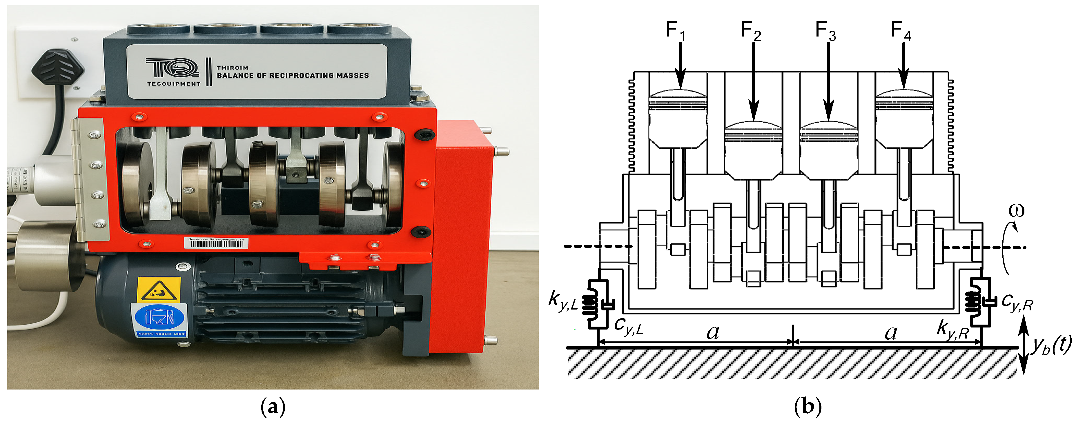
The base of the engine mounts is subjected to vertical excitation from chassis vibrations, denoted by yb(t). Unbalanced forces and torques acting on the engine are modelled as periodic functions containing multiple harmonics, which arise from engine firing events and crankshaft rotation. Introduce a as the half spacing (lever arm) from the engine centre of mass to each mount left and right relative deflections become
Equations (1) and (2) define the relative vertical displacement and velocity at the left and right engine mounts. They transform the global rigid-body motions, vertical translation y(t) and torsional rotation θ(t), into local mount deformations by accounting for the lever arm distance a and subtracting the base excitation yb(t). Translation affects both mounts equally, while rotation produces opposite vertical motions at the two sides. That geometric structure introduces inherent translation–torsion coupling. The velocity expressions in Equation (2) ensure that damping forces follow the same coupled pattern. The subscript L indicates the left-hand side, and R denotes the right-hand side. The system equations governing the dynamic model of four-cylinder automotive engine can be expressed as:
The nonlinear terms ky and cy represent mount behavior influenced by preload and geometric stiffening effects.
Crank angle differences between the cylinders:
Cylinder 1: θ1 = ωt
Cylinder 2: θ2 = ωt + π
Cylinder 3: θ3 = ωt + π
Cylinder 4: θ4 = ωt
Fu(t) represents the unbalanced vertical inertial force generated by the reciprocating components. The term mrrω2 follows directly from the kinematics of a slider–crank mechanism, where the reciprocating mass mr and crank radius r produce a periodic acceleration proportional to ω2 and modulated by the crank angle θi corresponding to the top dead center (TDC) position. TDC represents the position of the piston at the highest point of its stroke, closest to the cylinder head. It occurs when the crank angle θi is at 0° or 360° during a complete revolution. At TDC, the piston changes direction. It is either going up and about to come down or going down and about to come up. The second term, cos(2θi/n), accounts for the secondary inertial effects due to the finite connecting-rod ratio, which is l/r. Tc(t) is the combustion-induced torque, expressed as a harmonic expansion. In this expansion, Bn and ψn are the amplitude and phase of the n-th firing harmonic, respectively. The firing events introduce multi-harmonic periodic torque components that have shifted phases because they depend on the crank angle. Tu(t) is the definition of the unbalance torque that tends to create torsion. It is associated with the eccentric inertia Ie and a radius of eccentricity that generates a moment sinusoidal in nature and proportional to ω2. The expression reflects the moment generated when the center of mass of a rotating eccentric body deviates from the geometric axis.
Matrix formulation of coupled nonlinear dynamic system from Equations (3) and (4) becomes:
Equations (11)–(14) allow for nonlinear constitutive behavior in the mount and torsional elements. This means that, instead of having constant properties, the elements can have varying stiffness and damping that depend on the level of the input. The quadratic term means that these elements get stiffer with an increasing amplitude of relative motion. When the mounts are deflected more (meaning they’re working harder), they produce a restoring force that is more like a stiff spring. We think of this in two ways: (1) as preload effects in which the spring force grows with the amount of deflection, and (2) as stronger energy dissipation mechanisms coming into play with more rapidly oscillating (and hence more greatly displaced) mounts.
To model yb(t), the vertical base excitation, as a Gaussian random process, we define it as a stationary stochastic process with specified statistical properties such as mean, variance, and power spectral density (PSD).
A vertical base excitation acting on engine mounts rarely behaves like a clean harmonic input. Road irregularities, chassis vibrations, and environmental disturbances hit us in a disordered, broadband way. A Gaussian random-process formulation, as noted earlier, offers a mathematically consistent way to treat that variability while still permitting the system to be more or less tractable. Equation (15) states that yb(t) is drawn from a Gaussian process with mean μ and covariance function Ryb(τ). That choice implies that any finite collection of samples yb(t1), yb(t2), … follows a joint normal distribution whose structure is completely determined by the mean and covariance. The goal is to ensure that randomness enters the model through well-defined second-order statistics rather than ad-hoc noise. Equation (16) formalizes the mean level μ, which defaults to zero for road-induced motions once long-term drifts are removed. A zero mean assumption reflects the tendency of upward and downward fluctuations to cancel over time, even though instantaneous values may temporarily depart from the statistical centre. Equation (17) introduces the power spectral density Syy(ω). Only the frequency range ∣ω∣ ∣ωc∣ contributes to the energy content, which characterizes the excitation as band limited. That constraint mirrors actual vehicle environments, suspension systems and tyre-road interfaces do not pass arbitrarily high frequencies. The PSD plateau σy2 defines the variance per unit bandwidth, so the spectral shape directly controls how strongly different frequencies contribute to the vibration field. Equation (18) then gives a discrete-time update rule for synthesizing the process. The term −λyb(ti)Δt provides exponential decay (an Ornstein-Uhlenbeck structure), ensuring that the process remains stationary rather than drifting unbounded. The stochastic increment 2λσ2Δtξi injects random energy drawn from ξi ~ N(0,1).
3. Principal Component Analysis
In order to manage the high–dimensional vibration responses generated by the coupled nonlinear engine–foundation system, Principal Component Analysis (PCA) was employed. PCA is particularly suitable for resonance detection and coupled vibration analysis because resonance phenomena are often expressed as dominant modes of variability within multivariate vibration data. When the excitation frequency approaches a natural frequency of the system, the associated response components exhibit a marked increase in amplitude. PCA isolates these dominant patterns by concentrating the system variance into the first few principal components, which correspond to the most energetic vibration modes.
Constructing the multivariate data matrix Y as shown in Equation (19) involves stacking the time-domain vibration responses N sequentially. Each row of Y thus contains a full state vector of the coupled vertical-torsional system at one instant in time, with each physical variable residing in its own column. This arrangement makes it possible to perform correlation analysis on the output of the simulation, and it is especially suitable for use with principal component analysis. The reason it works so well with PCA is that the algorithm can only reveal and sort the dominant patterns when the variables are stored in a consistent and synchronized ensemble. Equation (20) performs a normalization step. It ensures that all variables enter the correlation analysis on a comparable scale by first centering them around 0 (by subtracting the mean vector μ) and then stretching them (by dividing, in this case, by the standard deviation σ). If we did not do this with our variables, when we computed the covariance matrix C expressed in Equation (21), the variables with the largest magnitudes would tend to mask any genuine dynamical coupling we might be interested in when we look at the matrix Ynorm right after we perform the normalization step, which is more appropriate when identifying resonance-driven variability. The principal components are obtained by projecting the normalized data onto the eigenvector matrix P (the eigenvectors are the same as the eigenmodes in this context). The resultant principal component score matrix is Z as denoted in Equation (22). The first column of Z contains the scores for the ‘first’ principal component, the second column contains the scores for the ‘second’ principal component, and so on. This ordering is done according to how much variance each component captures. Each row of Z tells how the system behaves in the corresponding direction, and large coherent oscillations in the first few components indicate the responsive modes of the system, which are responsible for resonance.
4. Adaptive Explicit Integration Framework for Nonlinear Engine Vibration Dynamics and Numerical Response Prediction
Numerical integration of the coupled translational and torsional equations of motion was performed using MATLAB R2024b’s built-in solver ode45, which implements an explicit Runge-Kutta Dormand-Prince method of orders 4 and 5 with adaptive step size control. ode45 employs an embedded Runge-Kutta pair in which the fifth-order solution is used to advance the state and the fourth-order solution is used to estimate the local truncation error; the difference between the two estimates informs the automatic adjustment of the internal time step to satisfy error tolerances during integration. By adapting the step size, the solver maintains accuracy without prescribing a fixed step, and it interpolates solutions onto the specified output time vector. In our implementation, time histories for response plots were generated on a uniform grid of 2000 points over 0 to 5 s (≈2.5 ms output spacing), and the spectral response was computed by evaluating the ODE on a nominal 1000 Hz grid over 5 s. At each grid, the solver’s dense output interpolates the adaptive integrations back to the desired uniform time sampling.
Table 1 summarizes the set of physical, structural, and excitation parameters adopted to characterize the coupled vertical–torsional engine-foundation model.
Table 1.
Simulation parameters.
The secondary inertia ratio n = 1/3, following typical values used in simplified rotary-mass models of multi-cylinder machines [29,30]. Cylinder phase offset angles were named as αi = {0, 2π/4, 4π/4, 6π/4} rad which distributes the four rotating masses at equal intervals over a complete revolution consistent with a uniform four-cylinder configuration. The applied combustion harmonic torque was represented by three retained harmonics with amplitudes Bn = [300, 120, 60] N·m and corresponding phase changes ψn = [0, 0.2, 0.5] rad that allows capturing high-order contributions while maintaining computational efficiency. The unbalance torque term with phase ϕ = 0 rad indicate that the torsional response remains in phase with the primary rotational motion of the system. The listed quantities define the inertial properties of the engine, such as elastic and dissipative behavior of the mounting system, external force and torque inputs used to excite the system.
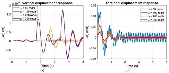
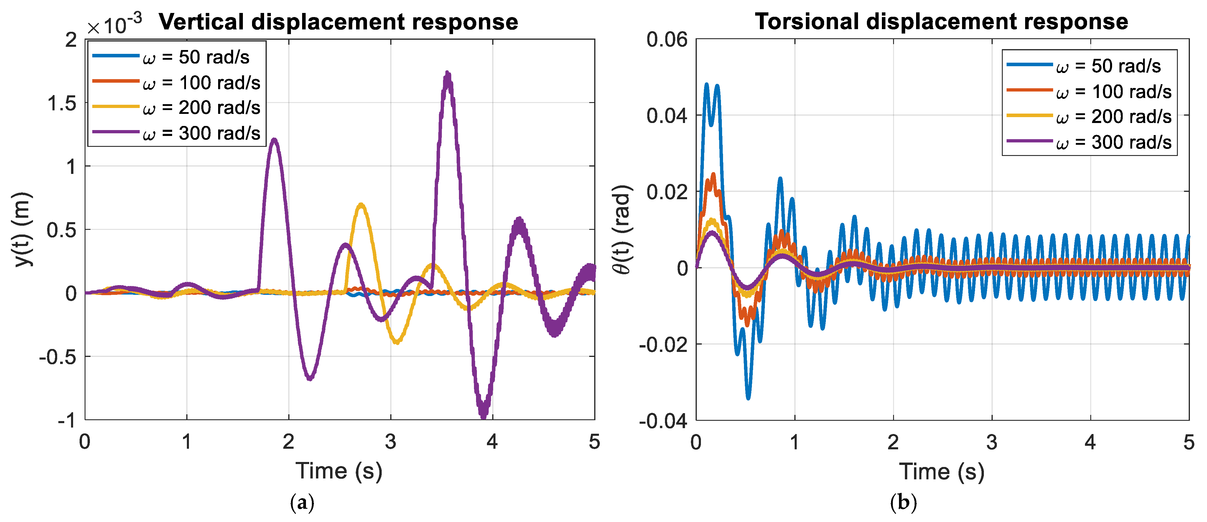
In Figure 2a, the vertical displacement exhibits the largest transient amplification at the lowest excitation speed when ω = 50 rad/s. The first peak reaches approximately 1.8 × 10⁻³ m before the response envelope contracts toward a steady oscillation of about 1.0 × 10⁻³ m. As ω increases to 100, 200, and 300 rad/s, both transient and steady amplitudes decrease systematically, with steady-subsystem. The effective dynamic stiffness is expressed as |ky − mω2 + jωcy|. For small state values ranging between 2 × 10⁻⁴ and 5 × 10⁻⁴ m. The response indicates a progressive transition away from the stiffness-controlled region of the translational coordinate. When ω is close to the natural frequency, the quantity ∣ky − mω2∣ diminishes and the damping contribution jωcy remains limited, producing lower effective dynamic stiffness and larger oscillation levels. With increasing ω, the inertia component mω2 escalates rapidly and governs the expression, accompanied by a proportional rise in jωcy. The combined effect is a larger magnitude of the complex stiffness, which reduces the displacement response. For large ω, therefore, both inertia and damping contributions elevate the effective dynamic stiffness, whereas for small ω the system remains more compliant. Figure 2b presents the torsional displacement response. A comparable transient phase appears, although the response is angular in scale. For ω = 50 rad/s, the initial peaks reach approximately 0.045–0.05 rad before decaying toward a steady oscillation below 0.01 rad. As ω increases, the steady angular amplitude decreases further, and at 300 rad/s the response is limited to a small bounded oscillation.
Figure 2.
Waveform response: (a) Vertical displacement y(t); (b) Torsional displacement θ(t).
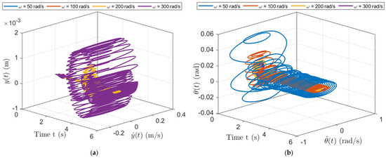
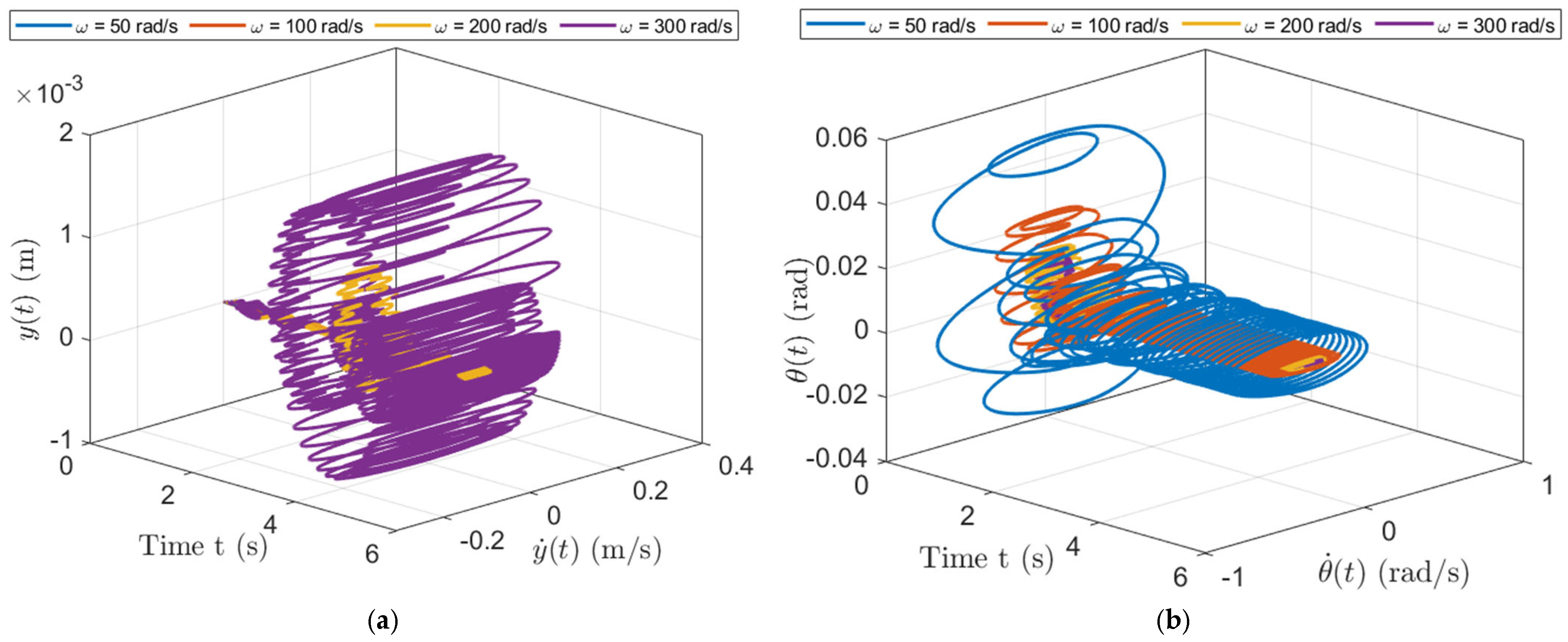
In Figure 3a, which depicts the vertical motion, the trajectory at ω = 50 rad/s initially moves outward, forming large loops in the (y,) plane. These wide spirals are evidence of the strong transient energy that accompanies this excitation. As we progress through time, the trajectory made by the moving system in phase space contracts; by the time we reach what should be the next excitation, we can approximate the loops contract progressively toward a cylindrical shape. This shape is what we would call in this context a steady-state orbit representation, meaning that it appears not to be spiraling outward or inward and also not to be oscillating or changing shape in any significant way. Indeed, for angular frequencies greater than or equal to 100 rad/s, the trajectories in phase space for the system under these vertical forcing conditions appear to converge much faster than they do at lower forcing frequencies. This means that the phase-space tube gets narrower and steadier for higher excitation frequencies. Moreover, as we discussed earlier, you can think of the radius of the spiral as determining or differentiating the oscillation modes of the system. For low frequencies, the system is wide, and for high frequencies, the system is narrow. But the width of the steady-state phase-space tube is also a way of talking about the helical structure of the oscillating system. Figure 3b shows the corresponding torsional trajectory in (θ,) phase space. Once again, the case with ω = 50 rad/s exhibits the largest initial loops, achieving angular displacements of nearly ±0.05 rad before tightening into a steady-state helix. In this instance, however, the winding is rather loose and the helix has a large radius, reflecting the considerable time it takes this trajectory to repeat. Indeed, all oscillatory trajectories in (θ,) space are comparatively stretched at this angular speed, since we have seen that going faster in the torsional direction produces smaller loops. The steady angular limit cycles remain narrow and regular for all speeds, with no evidence of quasiperiodicity or chaotic modulation.
Figure 3.
(a) Orbit pattern of the y(t); (b) Orbit pattern of the θ(t).
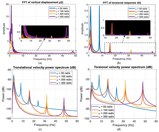
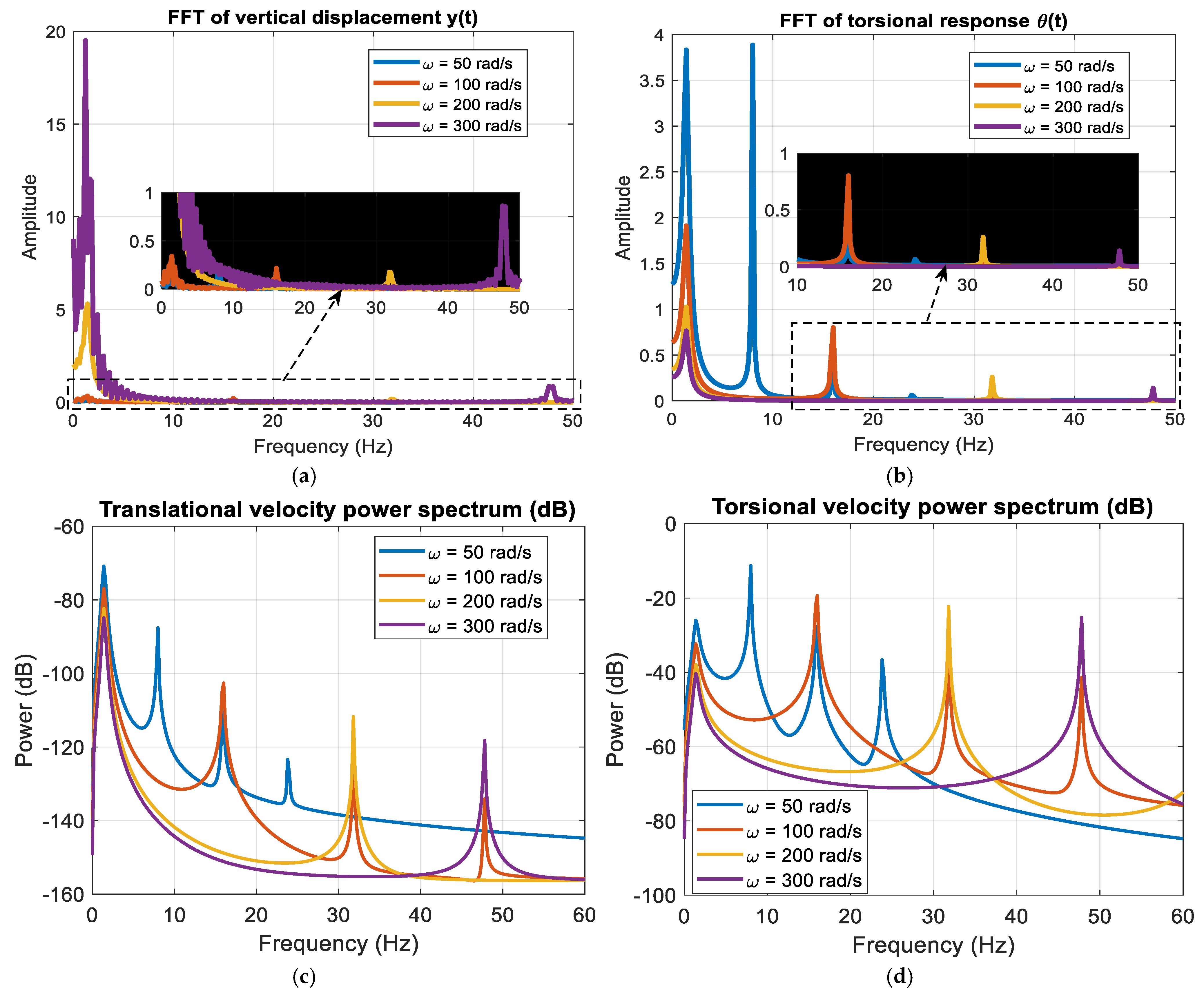
The largest spectral amplitude occurs at ω = 50 rad/s, consistent with the larger oscillations observed in the time domain. As ω increases, the peak amplitude reduces systematically. The cases at 50 rad/s and 300 rad/s appear to be an order of magnitude apart, which seems to suggest that the system is operating even farther from the translational compliance region than it was when exciting it at lower frequencies. Beyond that, the dynamic denominator’s growing with ω accounts for the steadily declining with π/2 out-of-phase peak in oscillator amplitude when exciting the system at higher and higher frequencies. Figure 4b displays the FFT of the torsional displacement. The same excitation-frequency peaks are present, confirming that both coordinates are driven by the same forcing structure. The 50 rad/s case again exhibits the strongest response, with the higher-speed cases displaying progressively smaller spectral peaks. The inset zoom shows that the vertical and torsional peaks align precisely at the engine-order frequencies, providing clear evidence of spectral translation-torsion coupling. Unbalance forces and combustion torque inject energy into both coordinate directions, with the mount geometry distributing the energy across the two spectra. Figure 4c,d show the power spectra of the translational velocity and the torsional velocity, respectively, on a (dB) scale. The dominant peaks in both panels occur near the excitation frequencies, with levels typically between −40 dB and −30 dB. However, the magnitude across both spectra decayed sharply away from those harmonics. In fact, levels fell below −90 dB for frequencies above roughly 60 Hz, giving a dynamic range of approximately 50 to 60 dB between the dominant peaks and the spectral background. The pronounced spectral decay away from the dominant peaks indicates efficient suppression of high-frequency components by the combined action of viscous damping and structural inertia, collectively interpreted as effective damping.
Figure 4.
(a) FFT of y(t); (b) FFT of θ(t); (c) Power spectrum of y(t); (d) Power spectrum of θ(t).
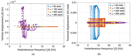
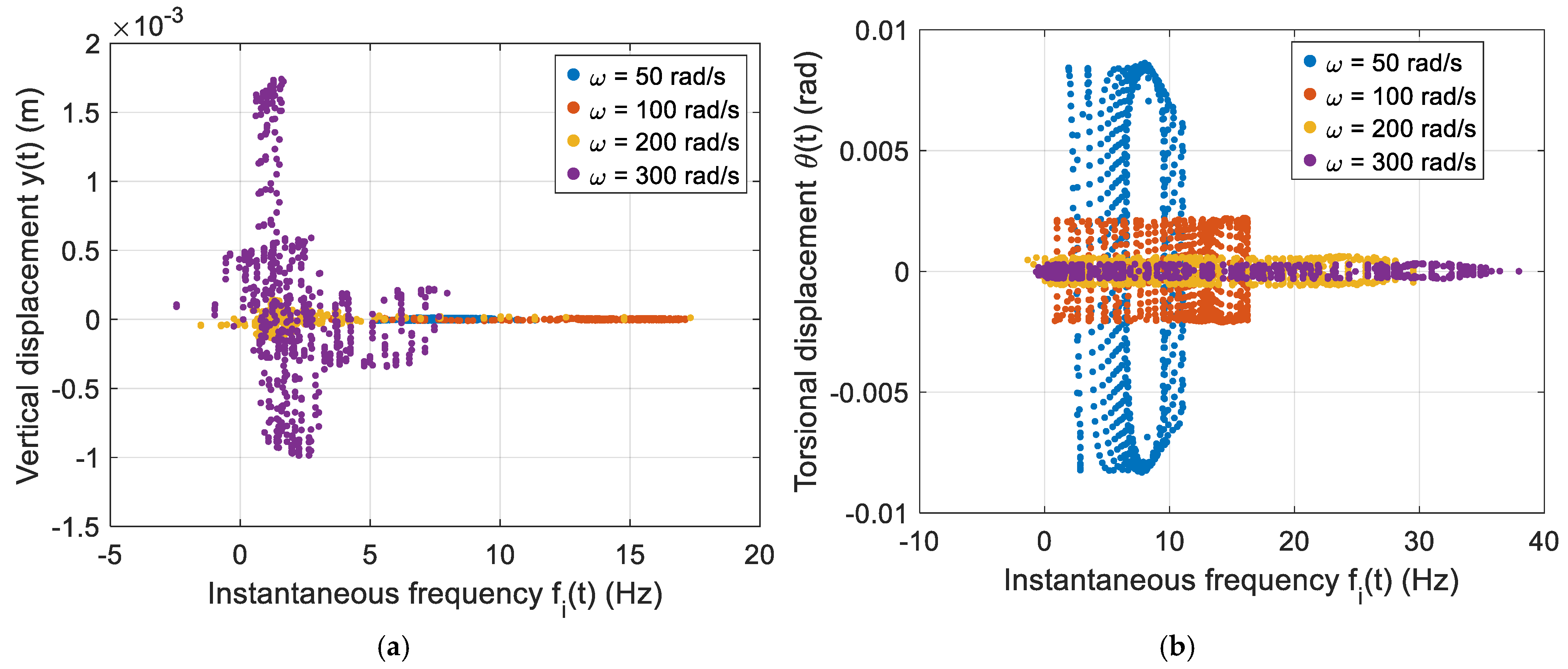
In Figure 5a, which corresponds to vertical displacement, the case of ω = 50 rad/s shows a widely spread, instantaneous frequency values during the transient stage. The cloud of IF points is diffuse across a loud band, indicating that multiple frequency components coexisted just after startup. This spread is a signature of the combined inertial forcing, mount compliance, and untouched nonlinear dynamics of translation and rotation response. In the initial part of the vertical displacement case, the term for horizontal damping cy is doing a lot of work to dissipate energy and establish steady-state behavior. In the initial part of this case and the next one, the dependence on gravity means there aren’t very good paths for energy to flow out of the system. So we’re almost entirely relying on cθ to establish the transient-to-steady-state transition. Rather, it indicates convergence toward a single dominant harmonic quasi-stationary mode characteristic of a forced perturbed periodic oscillator with a stable periodic attractor. Figure 5b presents the torsional instantaneous frequency dispersion, where for ω = 50 rad/s a pronounced initial spreading of the instantaneous frequency is observed, consistent with the transient behavior identified in the translational response. While the plot shows a broad distribution of frequencies during the early transient period, it also reveals a relatively steep distribution immediately following that period. The torsional oscillations have settled into a steady state resembling the forced, damped, nearly spherical harmonic oscillation that is a good approximation for the type of quasi-stable attractor expected under these conditions. It can also be seen that the spread of frequencies is more pronounced for the oscillations with a higher amplitude. In other words, the higher the engine order, the more likely to be observed some effect of the transition from an unforced damped oscillator to a forced single-mode oscillator.
Figure 5.
(a) y(t) Bifurcation map of IF; (b) θ(t) Bifurcation of IF.
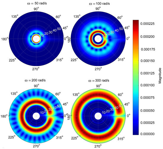
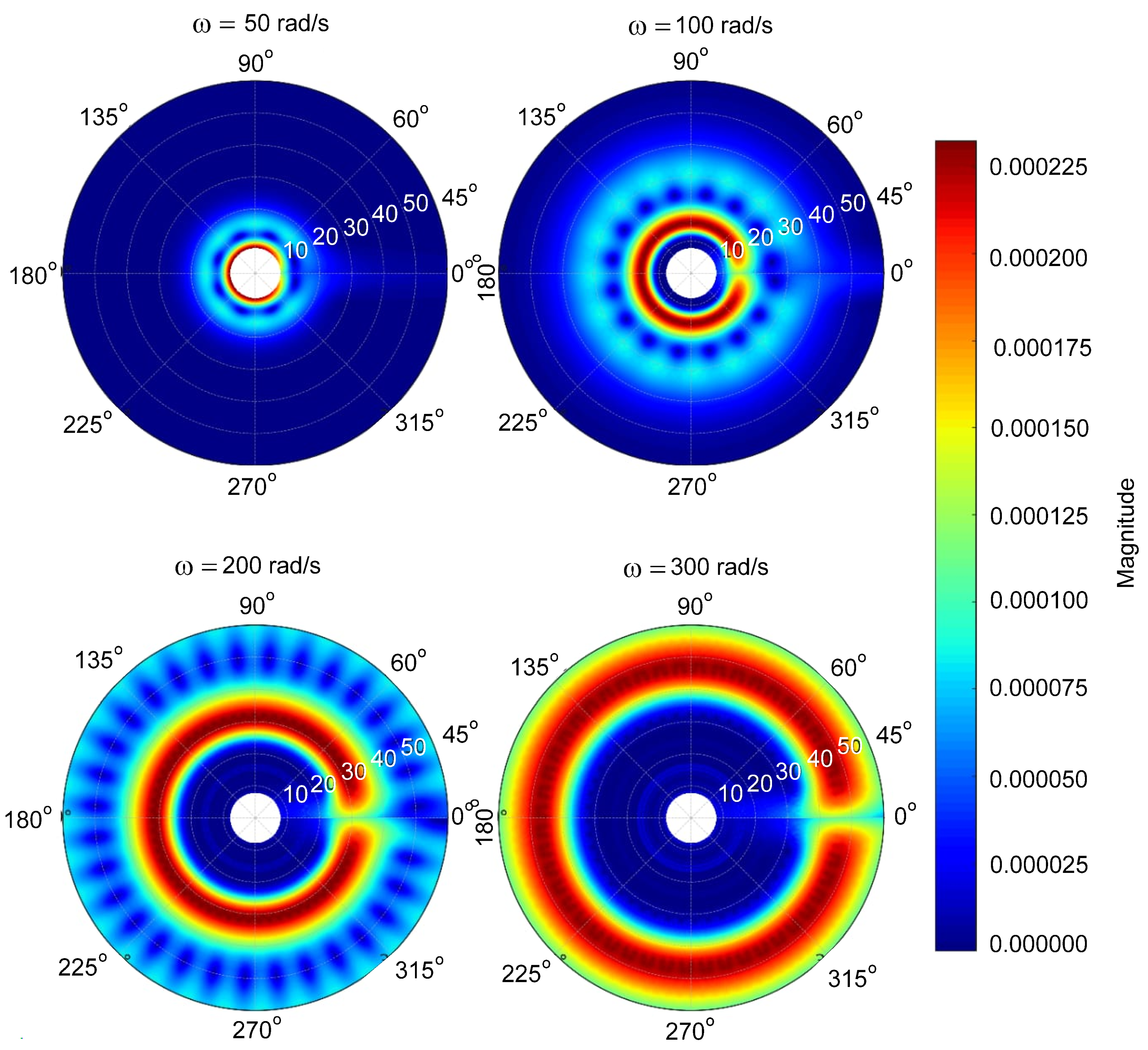
Figure 6 shows a clear progression in torsional energy organization across angular velocities from ω = 50 to 300 rad/s. Under the lowest speed condition, the scalogram presents a concentrated and nearly symmetric core of energy, characteristic of restrained torsional dynamics. At ω = 100 rad/s, a clear ring like structure forms, accompanied by angular modulation that signals stronger harmonic participation. Increasing to ω = 200 rad/s leads to noticeable radial growth and higher energy concentration, aligned with intensified forcing effects. By ω = 300 rad/s, the ring expands into a wide and nearly uninterrupted band, indicating a stabilized torsional response with strong phase coherence.
Figure 6.
CWT polar scalogram of torsional displacement.
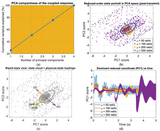
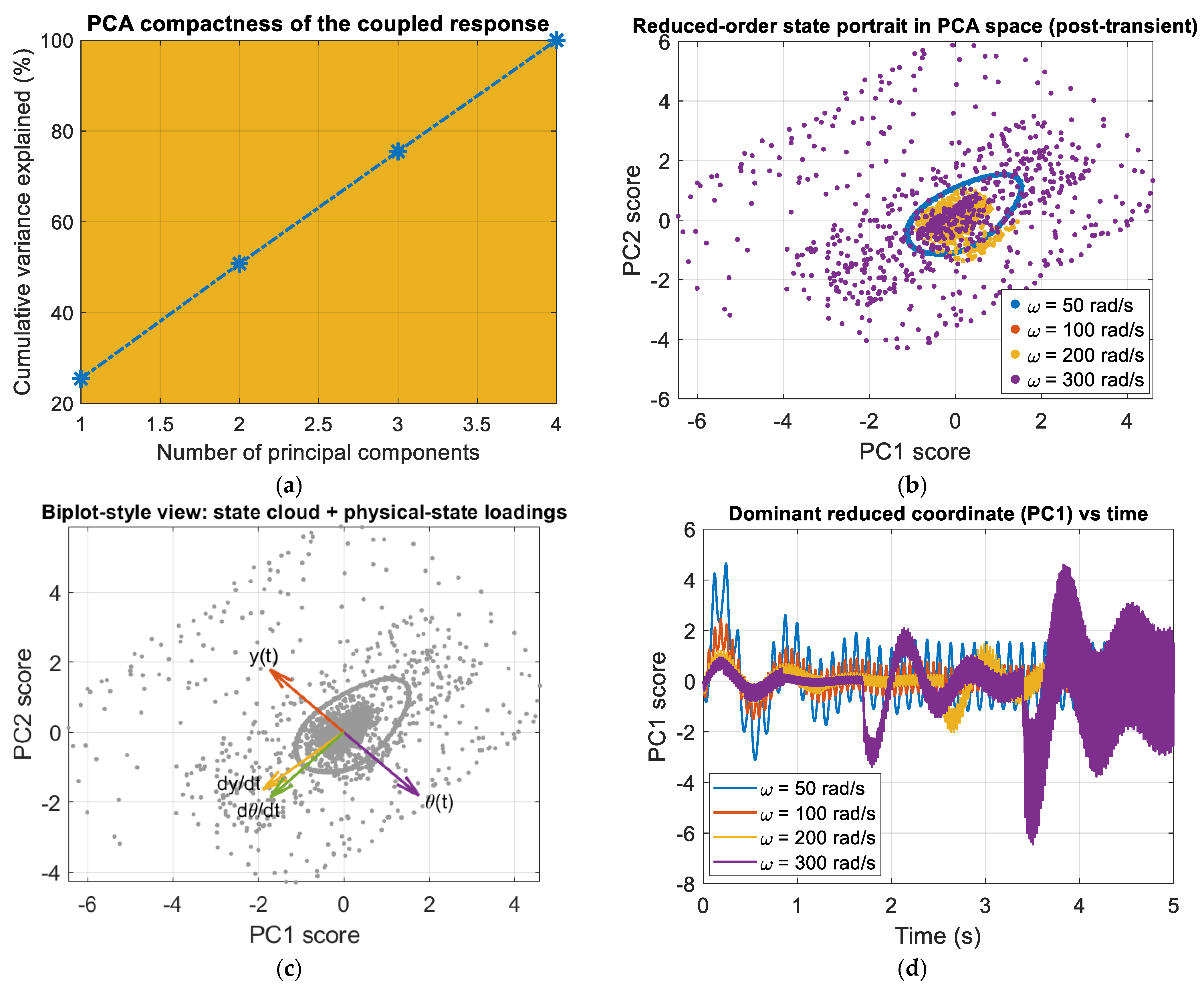
The most variance seen in Figure 7a is from the first two principal components, with PC1 alone explaining a large part of the total energy. The steep rise in the cumulative curve between the first and second components means that y(t), θ(t) and are strongly correlated. Such concentration confirms that the dominant vibration behavior is governed by a small number of coherent patterns rather than independent modal contributions. Figure 7b shows the portrait of the post-transient state in the PC1–PC2 plane. The cases of excitation form compact, closed clusters, confirming convergence to stable, periodic attractors in reduced space. The case at ω = 50 rad/s occupies the largest area, while increasingly higher excitation speeds produce clusters that are not only smaller in area but also denser a contraction that reflects the reduced steady-state amplitudes seen in both translation and torsion, and which clearly demonstrates that increasing excitation frequency does not change the attractor’s qualitative topology. Figure 7c projects the physical-state loadings onto the PC space. The separation of the loadings for the displacement variables and the velocity components indicates that the former aligns predominantly along PC1 and that the latter point in a different direction, or even a different set of principal components. Thus, it is implied, a dominating or even perhaps a large number of nearly coherent displacement modes of oscillation associate robustly with the PC1 pathway, whereas the velocity components associate with another less coherent set of pathways. Figure 7d shows the time evolution of the dominant principal coordinate (PC1). The oscillatory character of PC1 reflects the forced periodic nature of the system. All excitation speeds produce bounded oscillations, confirming stability. Across ω values, we see variations in amplitude and waveform density that suggest quantitative modulation of the dominant mode, but no qualitative transition such as bifurcation or development of chaotic behavior.
Figure 7.
PCA analysis of the coupled response: (a) cumulative variance explained; (b) post-transient state portrait in PC1–PC2 space for different excitation speeds; (c) biplot with physical-state loadings; (d) time evolution of the dominant principal component (PC1).
5. Finite Element Analysis of the Four-Cylinder Engine
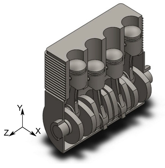
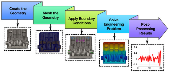
The main objective of this section is to extract intrinsic structural mode shapes and natural frequencies of the engine block geometry. Figure 8 portrays the compact four-cylinder engine geometry, captured in a CAD format that retains the essential aspects for finite element analysis. The piston aligns with the Y-axis, the crankshaft with the Z-axis, and the engine block with the X-axis. That coordinate system governs how modal vectors are interpreted after the structure has been discretized. For the four-cylinder engine installed on elastic foundations, FEA was used to model the complex behavior of the engine beyond what could be handled by a simplified coupled nonlinear model.
Figure 8.
Geometric layout of the engine block with piston, crankshaft, and global axes orientation.
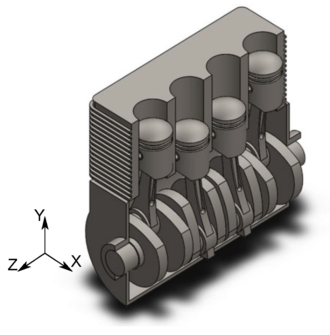
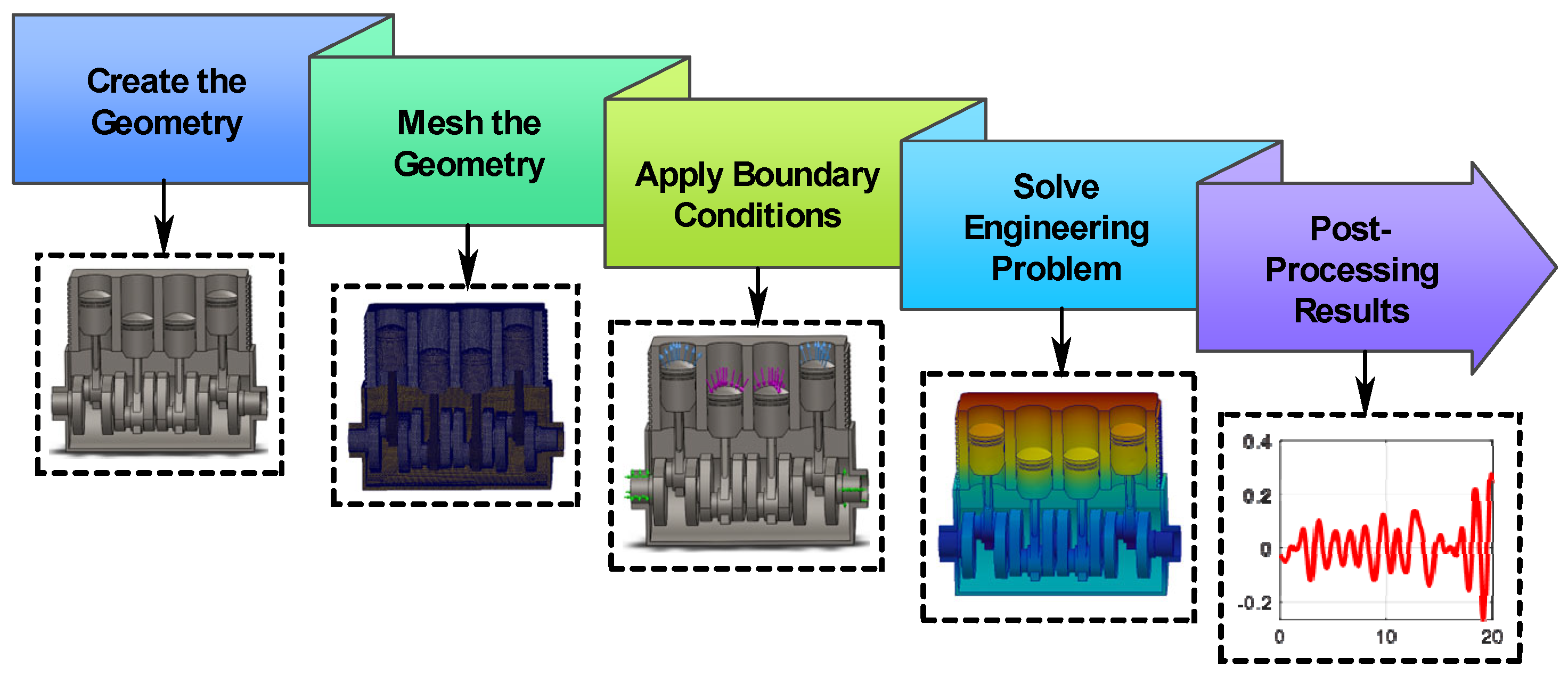
The lumped-parameter model describes the gross global motions of translation and torsion but, like any lumped model, does not incorporate mode shapes or account for coupling between the structural components of the engine. Breaking the engine block down into finite elements, includes material properties and geometric properties provides a much more realistic assessment of the vibration modes and resonance frequencies of the structure. Figure 9 illustrates the finite element modeling workflow, detailing how geometry creation, meshing, boundary condition setup, and numerical solving are integrated before the post-processing stage.
Figure 9.
Flow diagram of the FEA simulation process.
The diagram highlights the importance of each step in achieving a consistent and physically accurate model of the system. The finite element simulations were carried out using SolidWorks 2025, employing its frequency study module for modal extraction and structural evaluation. A solid finite element mesh based on a blended curvature-driven refinement scheme was implemented in the computational model. Overall, it presents a structured and reliable FEA approach for analyzing the engine’s dynamic behavior. Fixed support constraints were applied at the mounting points to mimic the attachment to viscoelastic mounts while allowing global deformation of the block.
Table 2 specifies a linear elastic isotropic steel material model, appropriate for capturing global vibration characteristics under elastic conditions. Table 3 confirms that the geometry is discretized using a high-quality mesh, with sufficient resolution and well-formed elements to support accurate simulation results. They indicate that both material representation and numerical discretization are sufficiently robust to support reliable dynamic and modal analysis results.
Table 2.
Material Properties.
Table 3.
Mesh information.
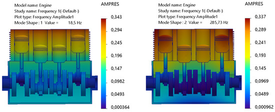
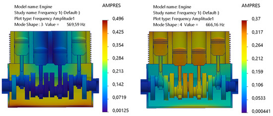
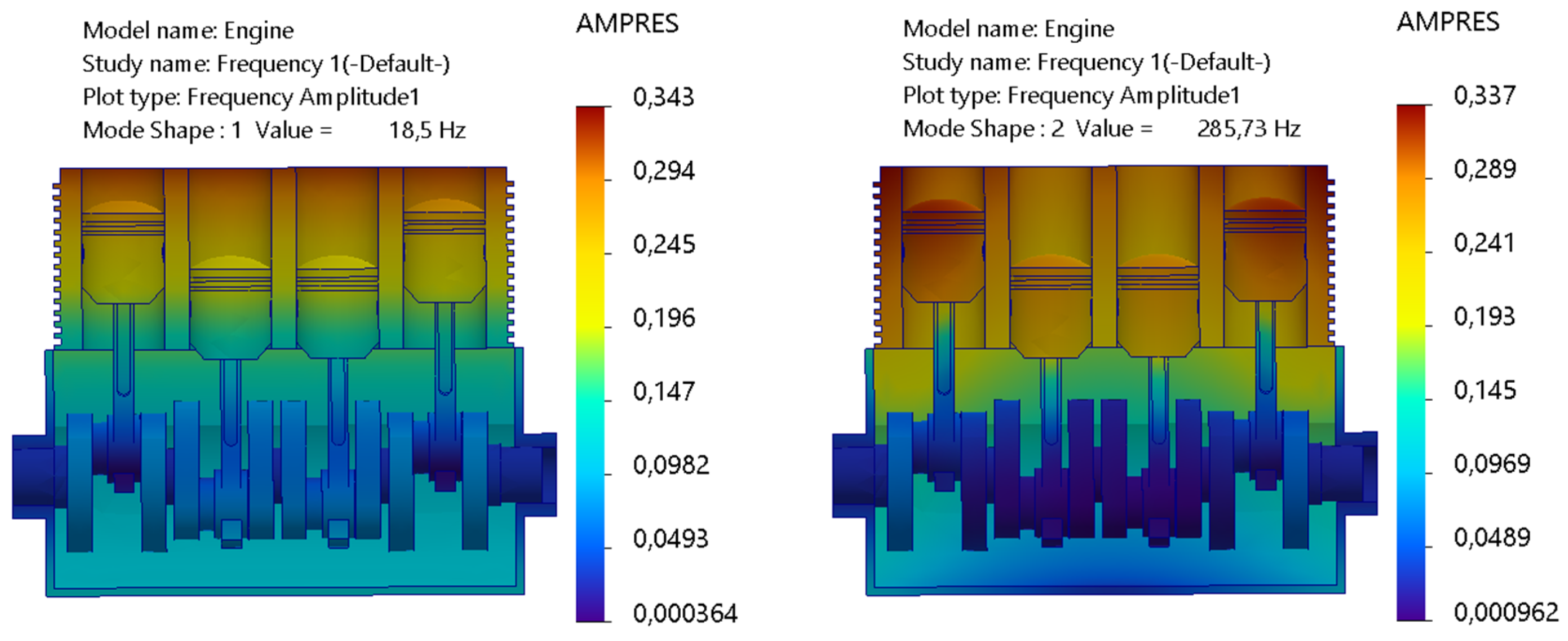
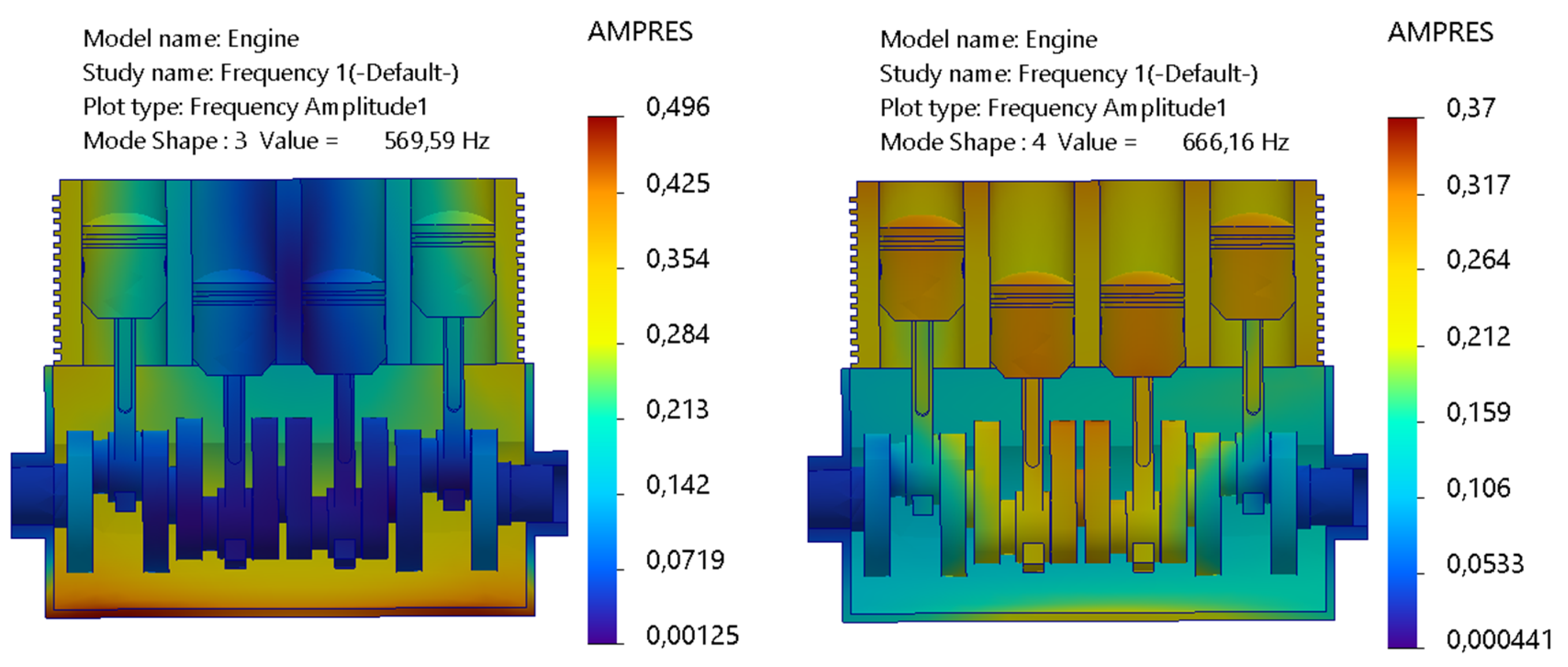
Figure 10 illustrates the deformation amplitude patterns of the first four vibration modes obtained from the finite element modal analysis of the engine structure. The outline traces how vibrational energy is spatially distributed by the machine block for each mode, while highlighting regions of dominant response. The first mode at 18.5 Hz exhibits a largely uniform, global deformation, characteristic of a low-order mode controlled primarily by global mass distribution and support conditions. The second mode at 285.73 Hz introduces stronger spatial gradients between the upper and lower regions of the block, while indicating increased involvement of internal structural features. At higher frequencies, deformation becomes more localized, with the third mode at 569.59 Hz showing concentrated response zones associated with bending and internal junction. The fourth mode at 666.16 Hz further accentuates this localization, while reflecting the increasing influence of hardness variations and geometric discontinuities.
Figure 10.
Amplitude results of first 4-modes of vibration.
Table 4 summarizes the normalized mass participation factors of the first four vibration modes and quantifies how modal inertia is distributed among the translational directions.
Table 4.
Mass Participation (Normalized).
The first mode at 18.5 Hz is dominated by motion in the X-direction, with a mass participation of 474.81 × 10⁻³, while contributions in the Y-direction (68.85 × 10⁻³) are smaller and the Z-direction participation (2.30 × 10⁻⁸) is negligible. The mode distribution verifies that the first mode is dominated by global translation in the translational direction, primarily along the X-axis. The second mode at 285.73 Hz indicates a marked change in the trend, where the mass is primarily involved in the Z-direction (567.93 × 10⁻³), with negligible involvement in the X-direction (6.83 × 10⁻⁷) and Y-direction (166.84 × 10⁻⁶). This indicates the onset of out-of-plane or vertical dynamics at this frequency. For the third mode at 569.59 Hz, the mass distribution becomes more widespread, with substantial involvement in the Z-direction (138.23 × 10⁻³) and Y-direction (4.52 × 10⁻³), with the X-direction being small (2.02 × 10⁻⁵). This indicates the increasing role of bending and deformation. The fourth mode at 666.16 Hz is dominated by motion in the Y-direction (654.02 × 10⁻³), with the X-direction (5.48 × 10⁻³) and Z-direction (357.28 × 10⁻⁶) being small. The trends of directionality are as expected for global translation in the first mode and bending-dominated modes for higher modes, as proposed by Dong and Shangguan 2023 [5]. The mode distribution indicates that the higher frequency modes are dominated by localized deformation in specific directions rather than global translation.
6. High-Dimensional Kernel Density Spectrogram
The spectrogram is defined as the square of the magnitude of the short-time Fourier transform and offers a deterministic view of signal energy over time and frequency. However, this approach can be sensitive to trade-offs in resolution. Kernel Density Estimation (KDE) offers a smoother, probabilistic alternative by calculating the underlying probability density of notable features without assuming a fixed parametric model. When extended to D-dimensional KDE spectrograms, this method supports the simultaneous analysis of multiple correlated dimensions such as time, frequency, amplitude, phase, space location, and sensor identity, creating a unified and scalable way to represent energy-focused features in high-dimensional signal spaces [31,32,33].
Multivariate kernel density estimator as used in Equation (23) maps the core vibration-related features from a D-dimensional space. The formulation computes the mean of N local kernel contributions, each weighted by the product of the bandwidth parameters hd. Such construction produces a density field assembled from smooth and overlapping components rather than isolated point concentrations, which is crucial when analyzing vibration signatures that vary continuously over frequency, amplitude, and modal coordinates. The kernel function Kd acts as the local weighting profile around each sample. Each observation is spread out into a neighborhood whose width is controlled by hd. Two basic kernel properties are established in Equation (24). These are unit integral and even symmetry. The first guarantees that the estimated density remains properly normalized and the second ensures that no directional bias is introduced along any feature dimension. Kernel density estimation can be extended by incorporating weights to highlight regions in the feature space associated with higher physically meaningful measures of signal energy, amplitude, or strength.
Kernel density estimation can be adapted to highlight high-energy or high-amplitude regions by attaching weights to each observation before smoothing. Signal-processing applications adopting this framework often report improved localization of energetic structures across time–frequency and multidimensional feature domains.
The estimator in Equation (25) is extended by introducing weights wi, which determine the contribution of each observation to the density field. Observations assigned larger weights exert a stronger influence on the resulting density distribution, shifting the representation toward a physically meaningful interpretation in which resonance-prone regions become more prominent. When all observations are treated equally, the estimator reflects a purely probabilistic view in which local resonant structures may be diluted within a nearly uniform background density. Applying weights increases separation between energetically dominant structures and low energy areas, which improves how the density distribution captures the governing dynamics. In this sense, the weighted formulation is able to provides information that help estimate the response of the system. Equation (26) specifies the bandwidth selection along each dimension. The smoothing parameter hd scales with the standard deviation of the corresponding feature is further adjusted by a factor involving the sample size N and the dimensionality D. Such scaling balances resolution and stability and the wider bandwidths reduce noise whereas narrower ones preserve modal ridges. Anisotropic tuning enables each feature to be smoothed according to its own variability. Across the engine block system, variations expressed through standard deviations reflect shifts in frequency response and amplitude modulation, assisting density estimation in maintaining sharp resonance localization while limiting numerical noise.
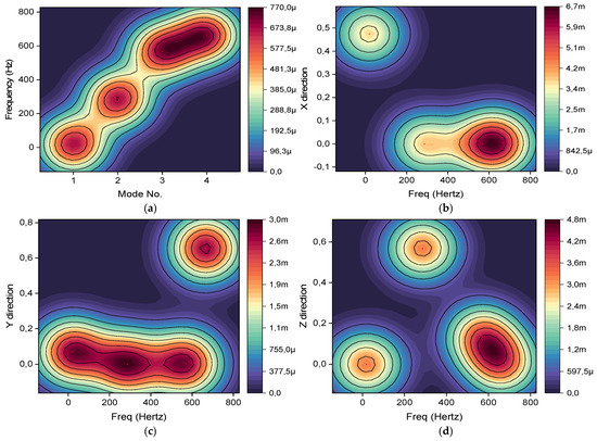
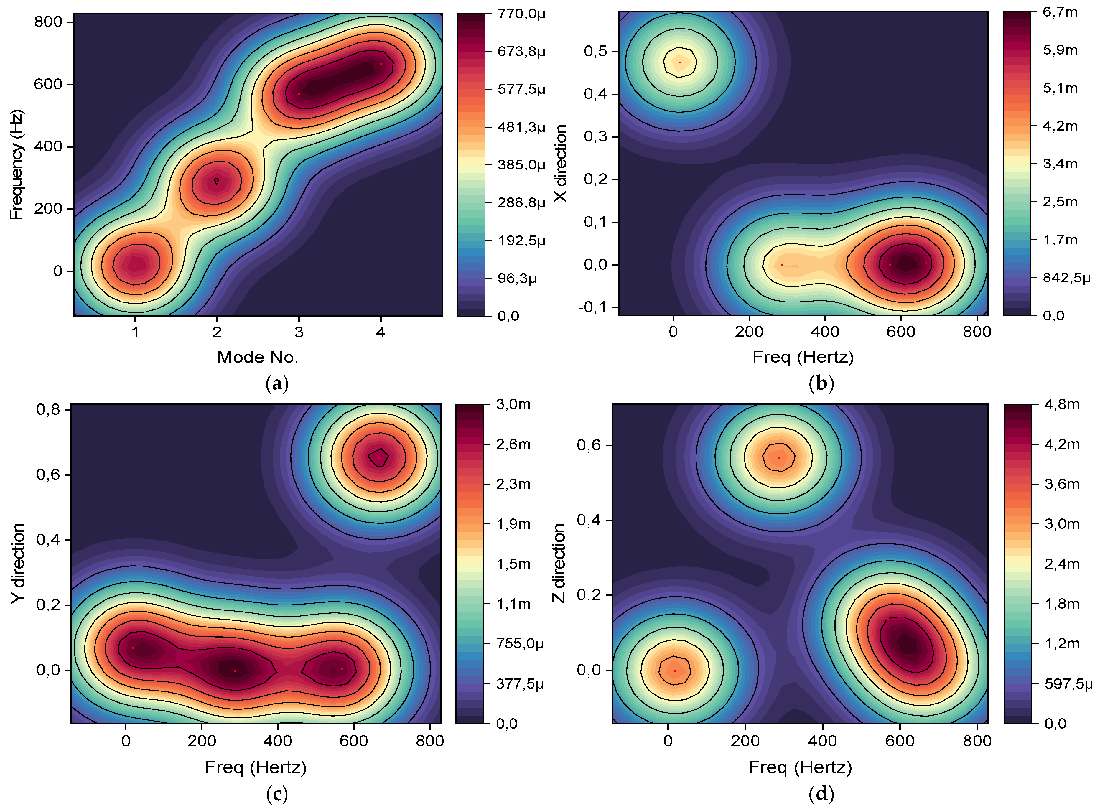
In Figure 11a, resonance frequencies increase progressively as modal index advances, culminating around 666.16 Hz for the highest computed modes. Growth does not occur in direct proportion to modal order; the upward curvature of the curve implies that structural stiffness plays an increasingly dominant role in the dynamic behavior. Mass participation factors provide further insight into how those modes are expressed spatially. In Figure 11b, participation in the X-direction is strongly concentrated at higher frequencies, particularly near 666.16 Hz, indicating a pronounced translational contribution along that axis. A broader frequency spread appears in Figure 11c for the X-direction. Participation extends across multiple bands, with the dominant peak occurring at a slightly shifted frequency compared to the X-axis, which points to a distinct directional sensitivity in the lateral response. Figure 11d presents the Z-direction behavior, where a comparable overall trend is observed; however, ridge mass participation is primarily concentrated within the intermediate frequency range, approximately 400 to 800 Hz. Such distribution suggests that modal energy is partitioned differently across spatial directions, revealing anisotropic characteristics in the vibrational behavior of the system.
Figure 11.
(a) Resonance frequency of each mode; (b) MPF at X-direction; (c) MPF at Y-direction; (d) MPF ant Z-direction.
7. Conclusions
A nonlinear vertical and torsional dynamic formulation was developed to describe the behavior of a four-cylinder engine mounted on a viscoelastic foundation. Geometric coupling between translation and rotation was explicitly introduced through mount deformation and lever arm interaction that allows vertical displacement and angular motion to evolve within a unified and mechanically consistent framework. Simulation outcomes demonstrated that increasing excitation speed suppresses transient overshoots and lowers steady state amplitudes, reflecting the influence of enhanced effective dynamic stiffness. Spectral analysis revealed that vibration energy remains confined to relatively narrow engine order frequency bands at higher speeds. Further understanding emerged from time frequency and modal investigations. Instantaneous frequency maps and phase trajectories indicated a tendency toward stable periodic attractors, reflecting progressive stabilization of the coupled motion under sustained excitation. Principal component analysis further revealed that the dynamics remain predominantly low dimensional, with most of the system variance captured by the leading modes. Finite element modal analysis of the complete machine geometry provided natural frequencies, mode shapes, and directional mass participation factors that align with the excitation range predicted by the nonlinear dynamic model. Density estimation was subsequently employed as a statistical descriptor to characterize resonance behavior and directional mass participation along the X, Y, and Z axes. Discrete resonance features were reformulated as continuous probability density distributions in the spectrograms, enabling systematic identification of key bands and sustained energy domains without sole reliance on peak based criteria. Future work will extend the framework toward stochastic road roughness modeling with controlled intensity scaling to investigate bifurcation thresholds and potential chaotic transitions. Coupled stress analysis using the validated finite element model will enable fatigue life prediction and failure assessment under resonant regimes. Experimental validation using vibration measurements from engine–mount test rigs is also planned to further verify the predictive capability of the proposed multi-scale analytical–FEA–KDE methodology.
Author Contributions
Conceptualization and initial development, D.F.S.; methodology, D.F.S., B.X.T. and A.A.A.; software, D.F.S., B.X.T. and A.A.A.; formal analysis of the data, D.F.S.; writing-original draft preparation, D.F.S., B.X.T. and A.A.A.; writing-review and editing, D.F.S., B.X.T. and A.A.A., and all those collaborating in the study. All authors have read and agreed to the published version of the manuscript.
Funding
This research received no external funding.
Data Availability Statement
The original contributions presented in the study are included in the article; further inquiries can be directed to the corresponding author.
Acknowledgments
The authors acknowledge the support from the Department of Industrial Engineering, Operations Management, and Mechanical Engineering, Vaal University of Technology, Vanderbijlpark, South Africa.
Conflicts of Interest
The authors declare no conflicts of interest.
Nomenclature
| Symbol | Definition | Unit |
| y(t) | Vertical displacement | m |
| θ(t) | Torsional rotation | rad |
| m | Engine mass | kg |
| J | Engine moment of inertia | kg·m2 |
| ky | Vertical stiffness | N/m |
| cy | Vertical damping coefficient | N·s/m |
| kθ | Torsional stiffness | N·m/rad |
| cθ | Torsional damping coefficient | N·m·s/rad |
| yb(t) | Vertical base excitation | m |
| Fu(t) | Unbalanced inertial force | N |
| Tc(t) | Combustion-induced torque | N·m |
| Tu(t) | Unbalance torque | N·m |
| mr | Equivalent reciprocating mass | kg |
| r | Crank radius | m |
| ω | Angular velocity | rad/s |
| l | Connecting-rod length | m |
| n = l/r | Rod-crank ratio | - |
| θi | Crank angle of cylinder i | rad |
| Bn | Combustion torque harmonic amplitude | N·m |
| Ψn | Phase of the n-th harmonic | rad |
| Ie | Eccentric inertia | kg·m2 |
| re | Eccentricity radius | m |
| ϕ | Phase of eccentric torque | rad |
| ky | Nonlinear vertical stiffness | N/m |
| cy | Nonlinear vertical damping | N·s/m |
| kθ | Nonlinear torsional stiffness | N·m/rad |
| cθ | Nonlinear torsional damping | N·m·s/rad |
| Syy | Power spectral density | m2/Hz |
| σy2 | Variance of base excitation | m2 |
| λ | Stochastic update factor | - |
| ξi | Standard normal random variable | - |
| PCA, PC1, PC2 | Principal components | - |
| Mode shapes | Normalized deformation shapes | - |
| MPF | Mass participation factor | - |
References
- Leliovsky, K.Y. Modeling of the total disturbing effects on the transmission elements from movement on different support bases and the engine. IOP Conf. Ser. Mater. Sci. Eng. 2021, 1086, 012026. [Google Scholar]
- Sharma, P.; Rao, N.; Wang, R.; Kakde, P. Predicting base Engine Vibrations using Flexible Multi Body Dynamics Simulation. ARAI J. Mobil. Technol. 2023, 3, 2023-JL-03. [Google Scholar] [CrossRef] [Scilit]
- Shi, C.; Liu, G.; Bian, Y.; Fan, M. Modeling and analysis on in-line four-cylinder vehicle engine system. In Eighth International Conference on Electromechanical Control Technology and Transportation (ICECTT 2023); SPIE: Bellingham, WT, USA, 2023; Volume 12790, p. 1279002. [Google Scholar]
- Wen, M.; Nguyen, V. Controlling isolation system of initial combustion engines. J. Mechatron. Artif. Intell. Eng. 2022, 3, 1–11. [Google Scholar] [CrossRef] [Scilit]
- Dong, G.Q.; Shangguan, W.B. Structural Vibration Analysis and Sound Quality Improvement for a Four-Cylinder Engine (No. 2023-01-1153). SAE Tech. Pap. 2023, 01, 1153. [Google Scholar]
- Ferreira, J.; Marin, B.; Lenzi, G.G.; Manuel, C.J.; Balthazar, J.M.; Lenz, W.B.; Kossoski, A.; Tusset, A.M. Neural Network Modeling and Dynamic Analysis of Different Types of Engine Mounts for Internal Combustion Engines. Sensors 2022, 22, 1821. [Google Scholar] [CrossRef] [Scilit]
- Ryzhikov, V.A. Resonance phenomena in vehicle suspension. In International Conference on Industrial Engineering; Springer Nature: Cham, Switzerland, 2023; pp. 641–649. [Google Scholar]
- Park, S.J. Comparative Study on Hyperelastic Constitutive Models for the Static and Dynamic Behavior of Resilient Mounts. Materials 2025, 18, 311. [Google Scholar] [CrossRef] [Scilit]
- Aikhuele, D.O. Note on the modelling of the frequency response of an engine mount based on the engine vibration. Eur. Phys. J. Plus 2021, 136, 727. [Google Scholar] [CrossRef] [Scilit]
- Lu, S.; Chen, Y.; Cao, H.; Zhao, G.; Zhang, H.; Guo, Y.; Li, W.; Ni, S.; Jiang, C. Coupling effect of shaft torsional vibration and advanced injection angle on medium-speed diesel engine block vibration. Eng. Fail. Anal. 2023, 154, 107624. [Google Scholar] [CrossRef] [Scilit]
- Li, S.; Li, Q.; Gao, S.; Chen, C.; Wang, W. A hybrid rotordynamic modeling method for a rotor system with flexible foundation and nonlinear support force: Numerical and experimental investigation. Mech. Syst. Signal Process. 2024, 208, 110975. [Google Scholar] [CrossRef] [Scilit]
- Chen, B.; Chen, L.; Zhou, F.; Huang, J.; Huang, Z. Prediction of frequency response of sub-frame bushing and study of high-order fractional derivative viscoelastic model. Sci. Rep. 2024, 14, 15767. [Google Scholar] [CrossRef] [Scilit]
- Martini, V.M.; Okabe, E.; Cavalca, K.L. On the experimental dynamic substructuring of rotating machine foundations. Mech. Syst. Signal Process. 2024, 206, 110921. [Google Scholar] [CrossRef] [Scilit]
- Zhang, J.; Lei, X.; Chan, P.W.; Dong, Y. Integrating physics-informed machine learning with resonance effect for structural dynamic performance modeling. J. Build. Eng. 2024, 84, 108627. [Google Scholar] [CrossRef] [Scilit]
- Slimak, T.; Zwölfer, A.; Todorov, B.; Rixen, D. A machine learning approach to simulate flexible body dynamics. Multibody Syst. Dyn. 2025, 64, 515–541. [Google Scholar] [CrossRef] [Scilit]
- Yin, J.; Liu, R.; Zhang, R.; Lv, B.; Meng, X. A new tribo-dynamics model for engine connecting rod small-end bearing considering elastic deformation and thermal effects. Tribol. Int. 2023, 188, 108831. [Google Scholar] [CrossRef] [Scilit]
- Kim, R.E. Classification of Variable Foundation Properties Based on Vehicle–Pavement–Foundation Interaction Dynamics. Sensors 2020, 20, 6263. [Google Scholar] [CrossRef] [Scilit] [PubMed]
- Zhu, G.; Cao, Q.; Wang, Z.; Zhang, Y.; Chen, Y.; Woo, K.C. Road to entire insulation for resonances from a forced mechanical system. Sci. Rep. 2022, 12, 21167. [Google Scholar] [CrossRef] [Scilit]
- Mirzaeian, M.; Langridge, S. Creating a virtual test bed using a dynamic engine model with integrated controls to support in-the-loop hardware and software optimization and calibration. Energies 2021, 14, 652. [Google Scholar] [CrossRef] [Scilit]
- Jane, R.; Rose, S.; James, C.M. Advancing Artificial Intelligence (AI) and Machine Learning (ML) Based Soft Sensors for In-Cylinder Predictions with a Real-Time Simulator and a Crank Angle Resolved Engine Model. Energies 2024, 17, 2731. [Google Scholar] [CrossRef] [Scilit]
- Garcia-Basurto, A.; Perez-Cruz, A.; Dominguez-Gonzalez, A.; Saucedo-Dorantes, J.J. Modeling and Prediction of Carbon Monoxide during the Start-Up in ICE through VARX Regression. Energies 2024, 17, 2493. [Google Scholar] [CrossRef] [Scilit]
- Ofner, A.B.; Kefalas, A.; Posch, S.; Geiger, B.C. Knock detection in combustion engine time series using a theory-guided 1-D convolutional neural network approach. IEEE/ASME Trans. Mechatron. 2022, 27, 4101–4111. [Google Scholar] [CrossRef] [Scilit]
- Dou, J.; Yao, H.; Li, H.; Wu, Y.; Yang, J. Torsional vibration suppression of a vehicle powertrain by a multi-stable nonlinear energy sink. J. Sound Vib. 2024, 589, 118594. [Google Scholar] [CrossRef] [Scilit]
- Omran, I.; Mostafa, A.; Seddik, A.; Ali, M.; Hussein, M.; Ahmed, Y.; Aly, Y.; Abdelwahab, M. Deep reinforcement learning implementation on IC engine idle speed control. Ain Shams Eng. J. 2024, 15, 102670. [Google Scholar] [CrossRef] [Scilit]
- Ma, X.; Shahbakhti, M.; Chigan, C. Connected vehicle based distributed meta-learning for online adaptive engine/powertrain fuel consumption modeling. IEEE Trans. Veh. Technol. 2020, 69, 9553–9565. [Google Scholar] [CrossRef] [Scilit]
- Gao, L.; Liu, S.; Xu, Z.; Li, B.; Cui, Y.; Meng, X. Tribo-dynamic modeling method and application to three-dimensional flexible PRL system. Int. J. Mech. Sci. 2024, 277, 109446. [Google Scholar] [CrossRef] [Scilit]
- Li, J.; Wan, T.; Huang, H.; Chen, G.; Liang, J.; Lei, B. Prediction and verification of performance and emission characteristics of diesel/natural gas dual-fuel engine based on intelligent algorithm. ACS Omega 2023, 8, 18212–18224. [Google Scholar] [CrossRef] [Scilit] [PubMed]
- Zuo, G.; Hou, L.; Lin, R.; Ren, S.; Chen, Y. Combination resonance and primary resonance characteristics of a dual-rotor system under the condition of the synchronous impact of the inter-shaft bearing. Sci. Rep. 2023, 13, 1153. [Google Scholar] [CrossRef] [Scilit] [PubMed]
- Kwak, S.W.; Shim, J.K.; Mo, Y.K. Kinematic conceptual design of in-line four-cylinder variable compression ratio engine mechanisms considering vertical second harmonic acceleration. Appl. Sci. 2020, 10, 3765. [Google Scholar] [CrossRef] [Scilit]
- Nainaragaram Ramasamy, M.; Slíva, A.; Govindaraj, P.; Nag, A. Topology optimization and testing of connecting rod based on static and dynamic analyses. Appl. Sci. 2025, 15, 2081. [Google Scholar] [CrossRef] [Scilit]
- Sozinando, D.F.; Tchomeni, B.X.; Alugongo, A.A. Modelling dynamic parameter effects in designing robust stability control systems for self-balancing electric Segway on irregular stochastic terrains. Physics 2025, 7, 46. [Google Scholar] [CrossRef] [Scilit]
- Chen, J.Q.; He, Y.L.; Cheng, Y.C.; Fournier-Viger, P.; Huang, J.Z. A multiple kernel-based kernel density estimator for multimodal probability density functions. Eng. Appl. Artif. Intell. 2024, 132, 107979. [Google Scholar] [CrossRef] [Scilit]
- Yang, J.Y. Exact Boundary Correction Methods for Multivariate Kernel Density Estimation. Symmetry 2023, 15, 1670. [Google Scholar] [CrossRef] [Scilit]

Disclaimer/Publisher’s Note: The statements, opinions and data contained in all publications are solely those of the individual author(s) and contributor(s) and not of MDPI and/or the editor(s). MDPI and/or the editor(s) disclaim responsibility for any injury to people or property resulting from any ideas, methods, instructions or products referred to in the content. |
© 2026 by the authors. Licensee MDPI, Basel, Switzerland. This article is an open access article distributed under the terms and conditions of the Creative Commons Attribution (CC BY) license.