


Abstract
This study aims to evaluate the effectiveness of sewage sludge ash (SSA) as a sustainable stabilizing agent for low-plasticity clay and to assess the applicability of machine learning techniques for predicting strength parameters. SSA was mixed with CL-type clay at contents of 0%, 5%, 10%, 15%, 20%, and 30% by dry weight. A comprehensive laboratory testing program was conducted, including Atterberg limits, compaction, fall cone, vane shear, and unconfined compressive strength (UCS) tests. The results showed that Atterberg limits increased with increasing SSA contents. As the SSA content increased up to 30%, the maximum dry unit weight decreased by approximately 6%, while the optimum water content increased by about 14%. The addition of SSA significantly enhanced the shear strength, with UCS-derived strength increments ranging from 264 to 771 kPa for 4-day-cured specimens and from 515 to 1351 kPa for 32-day-cured specimens. These findings demonstrate the strong potential of SSA as an alternative and sustainable soil stabilizer. In addition, Self-Organizing Maps (SOMs) were employed to analyze the distribution and relationships of parameters within the experimental dataset, followed by Support Vector Machines (SVMs) for classification and prediction. Using the experimental results, the undrained shear strength parameters obtained from fall cone (su-FCT) and laboratory vane shear (su-LVT) tests were predicted with accuracies of 83% and 79%, respectively. The novelty of this study lies in the integrated experimental–data-driven framework, in which extensive laboratory testing is combined with machine learning methods to both validate and reliably predict the strength behavior of SSA-stabilized clay.
1. Introduction
Population growth has led to an increase in the production of sewage sludge from wastewater treatment plants all over the world. One of the main outputs from a wastewater treatment plant is sewage sludge. The volume of sewage sludge has been increasing rapidly over time, and it is expected to rise further because of the increase in urbanization. The fact is that disposing of sewage sludge material is a challenging problem that has emerged in recent years [1,2,3]. Today, two main approaches, namely land filling or cement blending, for the disposal of sewage sludge have been widely used across the world [4,5,6,7,8,9,10,11,12,13].
In addition, sewage sludge incinerators have been recently adopted in wastewater treatment plants as an alternative disposal technique in order to decrease the large volume of sewage sludge through a combustion process [14]. Perez et al. [15] and Ciaran et al. [16] proved that the incineration process reduces the volume of sewage sludge by up to 90%. The main chemical components of sewage sludge ash (SSA) produced at the end of this process include silicon dioxide (SiO2), calcium oxide (CaO), and aluminum oxide (Al2O3), which are also present in the chemical composition of ordinary cement [17,18]. This similarity has led to the use of SSA in cement/concrete-related studies in the literature [19,20,21,22,23,24]. Al Sayed et al. [25] and Merino et al. [26] proposed the use of SSA in asphaltic paving mixtures and in glazed tiles, respectively. Moreover, SSA has been introduced as an alternative material to be mixed with cement or hydrated lime in order to improve the stability of soft soils [27,28,29,30,31,32]. Chen and Lin [33] used SSA and cement together at a ratio of four to one to stabilize a cohesive subgrade soil and reported that the UCS values of treated specimens increased by about three to seven times, whilst the California Bearing Ratio (CBR) performance was increased by up to 30 times greater than that of untreated soil. The UCS tests carried out by Tempest and Pando [34] indicated a substantial increase in stiffness and bearing capacity values by adding SSA into a clay at varying ratios. Many researchers working on the use of SSA in various geotechnical engineering applications have reached similar findings [30,35].
Various soil improvement techniques aimed at increasing the shear strength and reducing the deformability of weak soils have been widely used in geotechnical engineering. Considering the key papers pointed out above, a comparative analysis of extensive laboratory studies on the mixtures of clay with SSA has been conducted using Atterberg’s limits, compaction, fall cone, vane shear, and unconfined compressive strength test results. This is the first study to present such an extensive comparative investigation, which proposes the use of SSA as a sustainable stabilizing agent in low-plasticity (CL) clay. SSA grains that passed through a 0.425 mm diameter sieve were mixed with the clay at ratios of 0%, 5%, 10%, 15%, 20%, and 30% by dry weight. These specimens were studied by employing an extensive series of laboratory tests (Atterberg’s limits, compaction, fall cone, vane shear, and unconfined compressive strength) for the purpose of evaluating SSA as a sustainable additive for soil improvement. Finally, two innovative data processing methods were also employed on the dataset obtained from the experimental works for the classification and prediction of soil characteristics.
2. Materials and Method
2.1. Clay
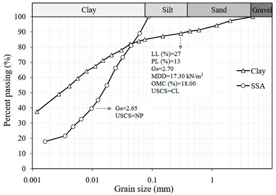
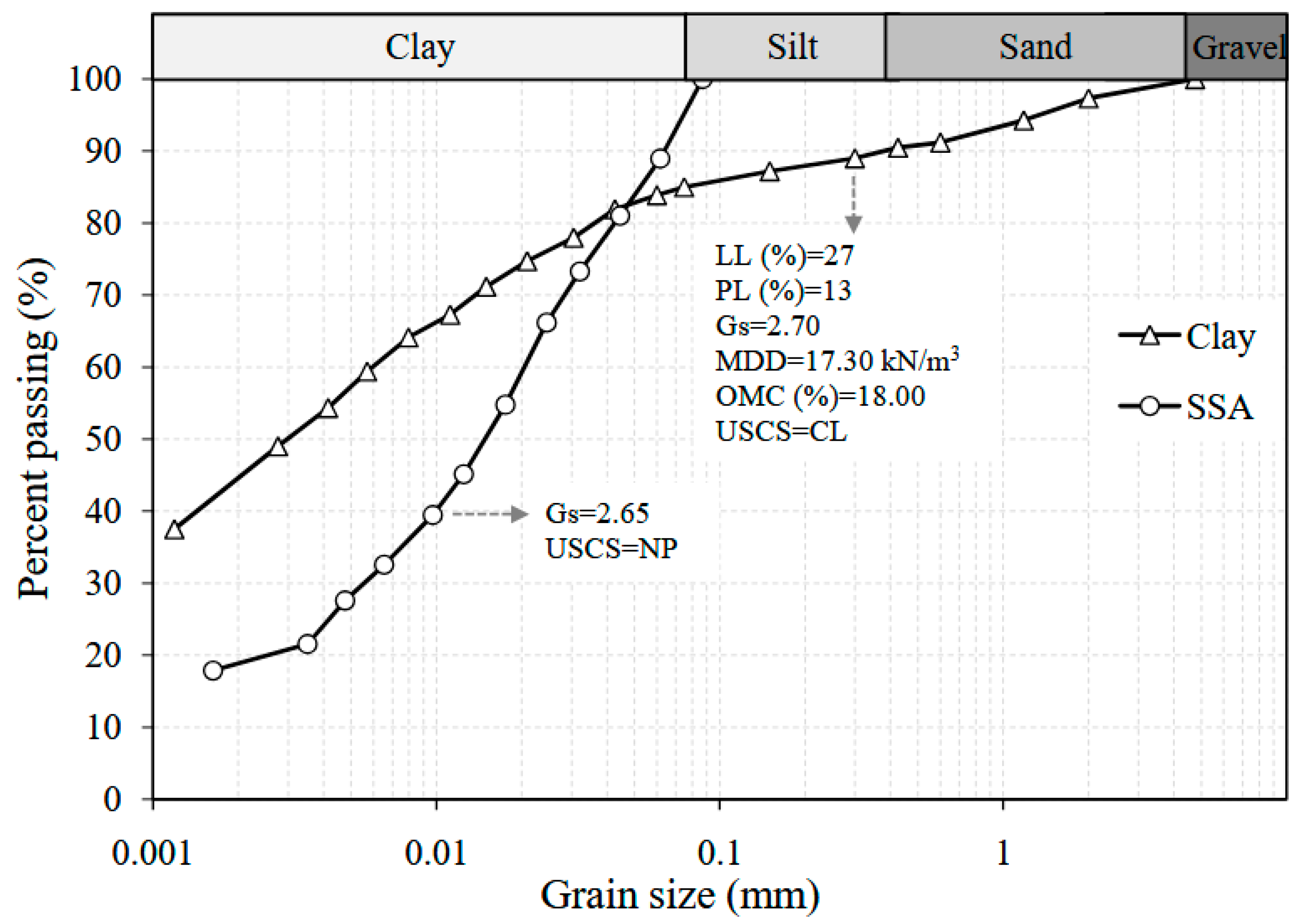
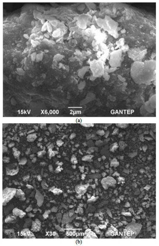
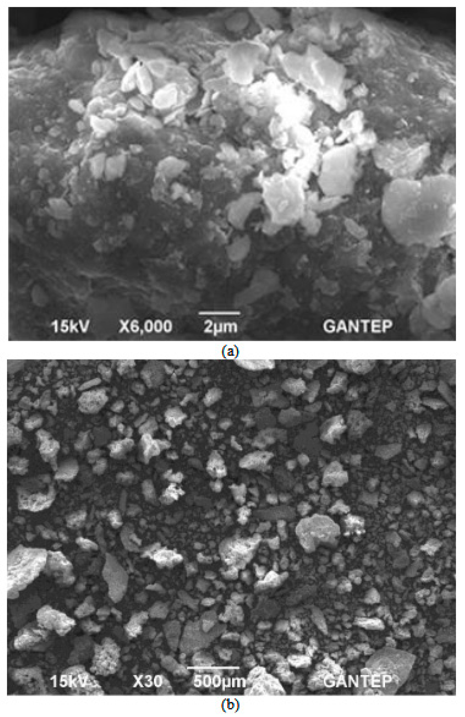
The type of soil used in this study was a low-plasticity clay (CL) obtained from the Gaziantep University campus, Turkey. The grain size distribution of this soil was determined in accordance with the ASTM D422 [36]. The plastic limit and liquid limit values were found to be 13 and 27, respectively [37]. The specific gravity of the clay was 2.70. The grain size distribution and Scanning Electron Microscope (SEM) pictures of the clay grains are displayed in Figure 1 and Figure 2a, respectively.
Figure 1.
Grain size distribution curves of the clay and SSA samples used during the experimental studies.
Figure 2.
Scanning Electron Microscope (SEM) picture of the (a) clay sample and (b) sewage sludge ash (SSA) sample used during the experimental studies.
2.2. Sewage Sludge Ash (SSA)
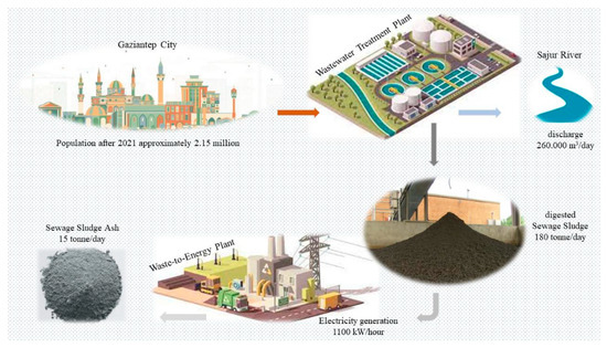
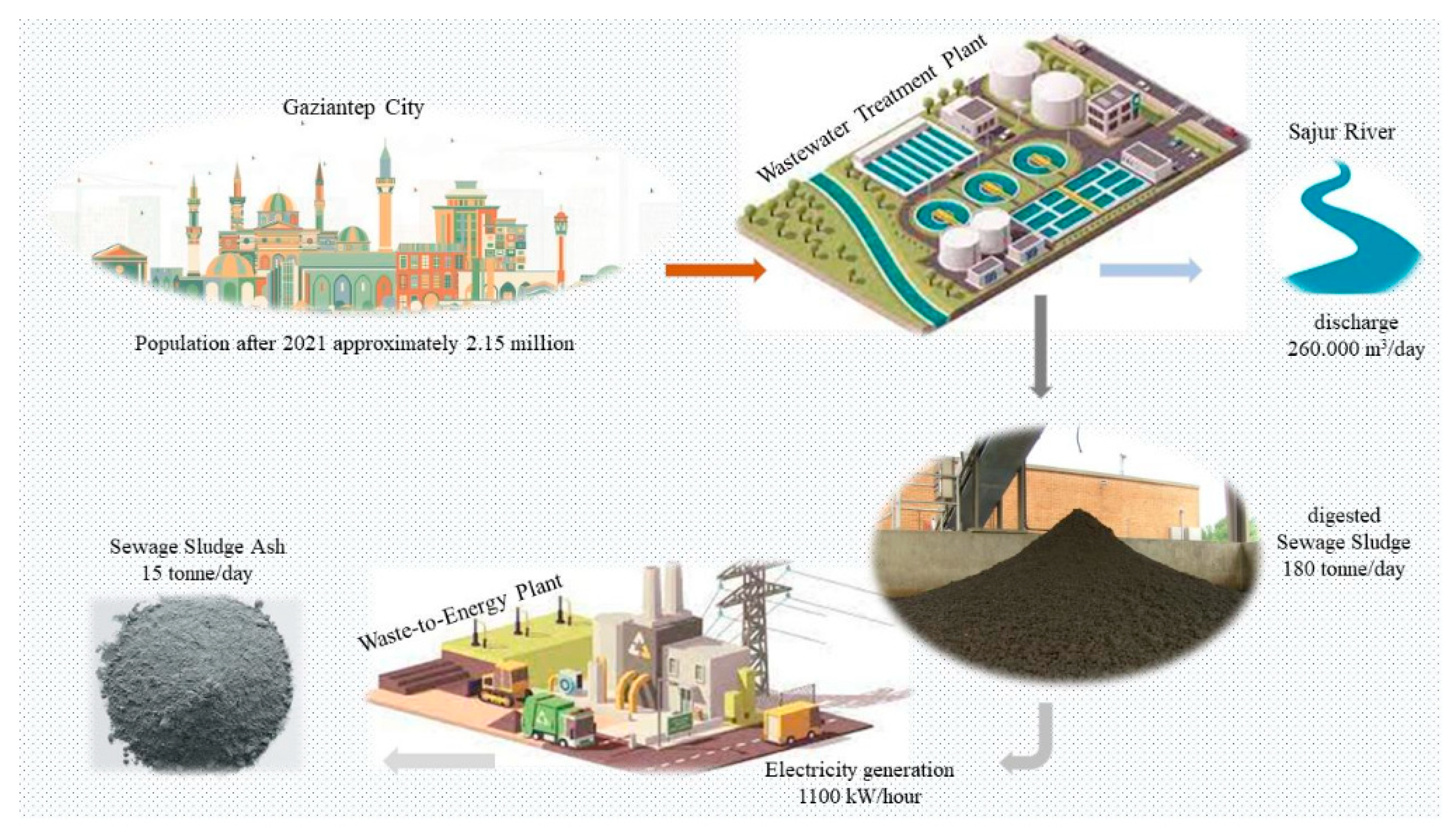
The SSA used in the present work was collected from the wastewater treatment plant of Gaziantep water and sewerage administration (GASKI), which was established in 1999 and today services a population of around 2.5 million. The plant treats about 260.000 m3 of sewage sludge per day and discharges it into the Sajur River. Following the discharging process, about180 tons of the digested sewage sludge remaining is transferred to the digestion tanks for the incineration process at high temperature levels, and then about 15 tons of ash (SSA) is produced per day. The thermal energy released during the incineration process is also used to generate electricity, which amounts to approximately 1.100 kW per hour. The whole process is summarized in Figure 3. The specific gravity of the SSA grains was found to be 2.65. The grain size distribution was defined by employing the ASTM D422 [36] (Figure 1). The SEM picture of the SSA is presented in Figure 2b.
Figure 3.
A simplified graphical abstract of the SSA formation.
Some properties and the X-Ray Fluorescence (XRF) analysis of the clay and SSA used during the experimental works are also provided in Table 1 and Table 2.
Table 1.
Properties of the materials used during this study.
Table 2.
X-Ray Fluorescence (XRF) analysis of clay and SSA.
2.3. Specimen Preparation and Testing
The specimens were prepared by mixing the clay and SSA at the ratios of 0%, 5%, 10%, 15%, 20%, and 30% by dry weight and then tested by employing the Atterberg’s limits, compaction, fall cone (FC), laboratory vane shear (LVS), and unconfined compression strength (UCS) testing machines in accordance with the standards ASTM D4318-17e1, ASTM D698-12 (2021), BS 1377-2, ASTM D4648-08, and ASTM D2166-06, respectively [37,38,39,40,41]. In order to evaluate the influence of curing time on the UCS testing result, the specimens tested on these machines had been left in a plastic bag over various days to cure (4, 8, 16, and 32 days).
3. Experimental Results and Discussion
3.1. Effect of SSA on Atterberg’s Limits
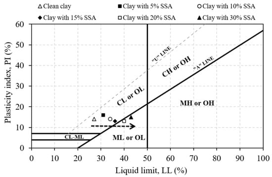
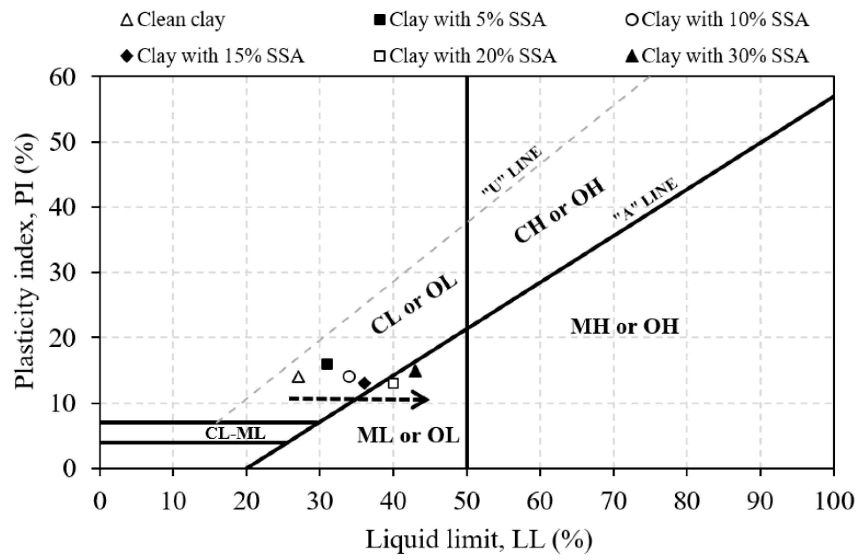
The SSA grains were added at various percentages (from 0% to 30%) by the dry weight of the samples and mixed with the clay, which passed through a 0.425 mm diameter sieve. The liquid limit of the clean clay increased from 27% to 43% by the increment of SSA contents up to 30%, whilst plastic limits of the same specimens were changed from13% to 28%. The Atterberg’s limits testing results of the mixtures tested are shown in Figure 4, which indicates that the mixtures with more SSA grains have a trend of changing from the CL to ML type of soil. It should be emphasized that all Atterberg’s limits tests were conducted without any curing period. Therefore, the observed changes reflect immediate index change effects associated with the physical interaction between the SSA particles and clay, rather than true stabilization resulting from time-dependent chemical reactions. Consequently, the observed classification shifts should not be over-interpreted as evidence of long-term soil stabilization. The XRF analysis shows that the SSA is richer in CaO, SO3, and P2O5, while clay contains more SiO2, Al2O3, and Fe2O3. Their initial interaction is dominated by physical effects, such as particle replacement and size distribution changes, affecting the water demand and consistency. Calcium-rich SSA can induce cation exchange and flocculation, causing short-term plasticity changes. However, due to its lower reactive silica and alumina and the absence of curing, chemical stabilization is limited, with time-dependent reactions occurring only under prolonged curing and moisture conditions. In light of the previous studies [28,34,42,43,44,45], the authors’ interpretation is that the SSA samples used exhibit a non-plastic to medium plastic characterization in the Atterberg’s limits tests, which were carried out without any curing time. This behavior requires great caution in the design of structures likely to be exposed to water, such as water-retaining structures [3]. The XRF, specific gravity, and particle size data indicate that SSA and clay differ in chemical composition and grain diameter, providing meaningful insight into their short-term physical and chemical interactions, even though additional descriptors like the mineral phases, amorphous content, pozzolanic reactivity, pH/alkalinity, and surface area could further refine long-term predictions.
Figure 4.
The effect of the SSA content on the Atterberg’s limits.
3.2. Effect of SSA on Standard Proctor Results
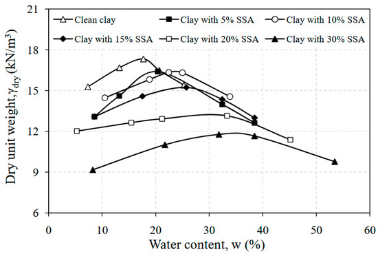
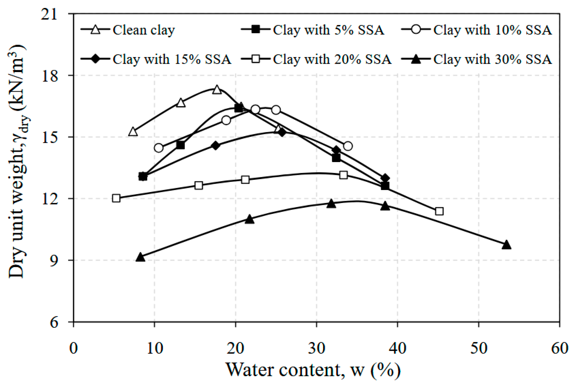
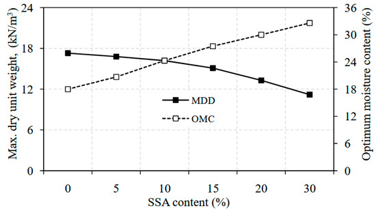
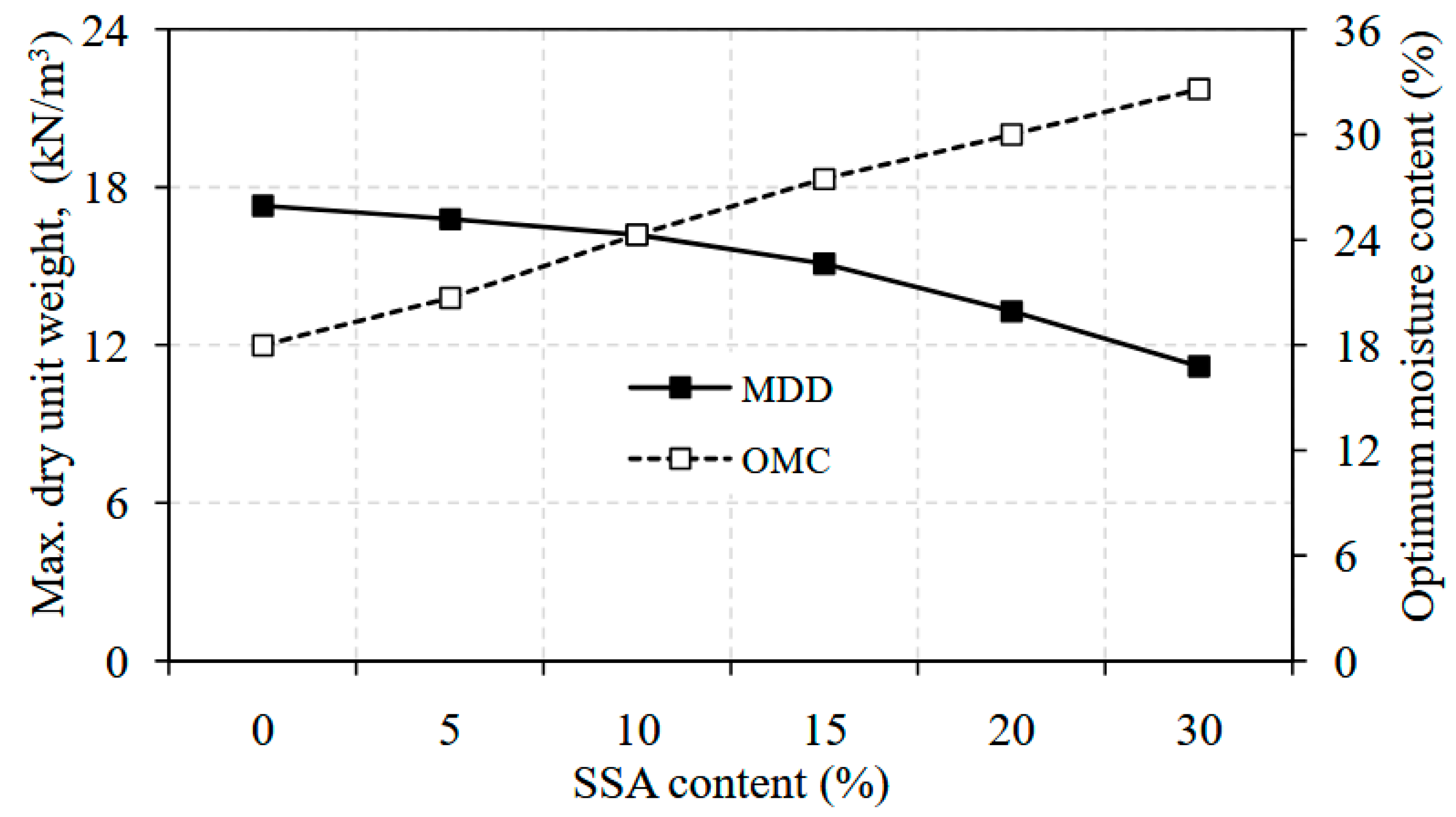
A series of standard proctor tests were performed on the clay and clay–SSA mixtures at different percentages from 0% to 30% by the dry weight of the mixture. The compaction curves obtained at the end of this experimental study are shown in Figure 5. It is seen that the maximum dry density (MDD) of the clay and SSA mixtures decreased from 17.7 kN/m3 to 11.8 kN/m3 as the amount of SSA increased up to 30%.This might be because of the increase in the void ratio, as well as the less specific gravity value of the SSA grains. In addition, it is also likely to be due to the chemical composition of SSA grains, leading to a high water absorption capacity of the mixtures [46]. Evidently, it was observed that the sensitivity of the mixture to water decreased depending on the amount of SSA added. Ingunza et al. [29] pointed out similar findings, where the MDD values were observed to substantially decrease when adding SSA samples into the mixtures up to 30%, whilst the OMC values increased from about 18% to 33% with the same level of SSA addition (Figure 6).The results of the study by Al-Sharif and Attom [28] were found to be in a harmony with the case described herein.
Figure 5.
Standard proctor testing results for the clay–SSA mixtures.
Figure 6.
The effect of the SSA content on the MDD and OMC values.
3.3. Effect of SSA on Fall Cone Testing Results
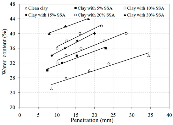
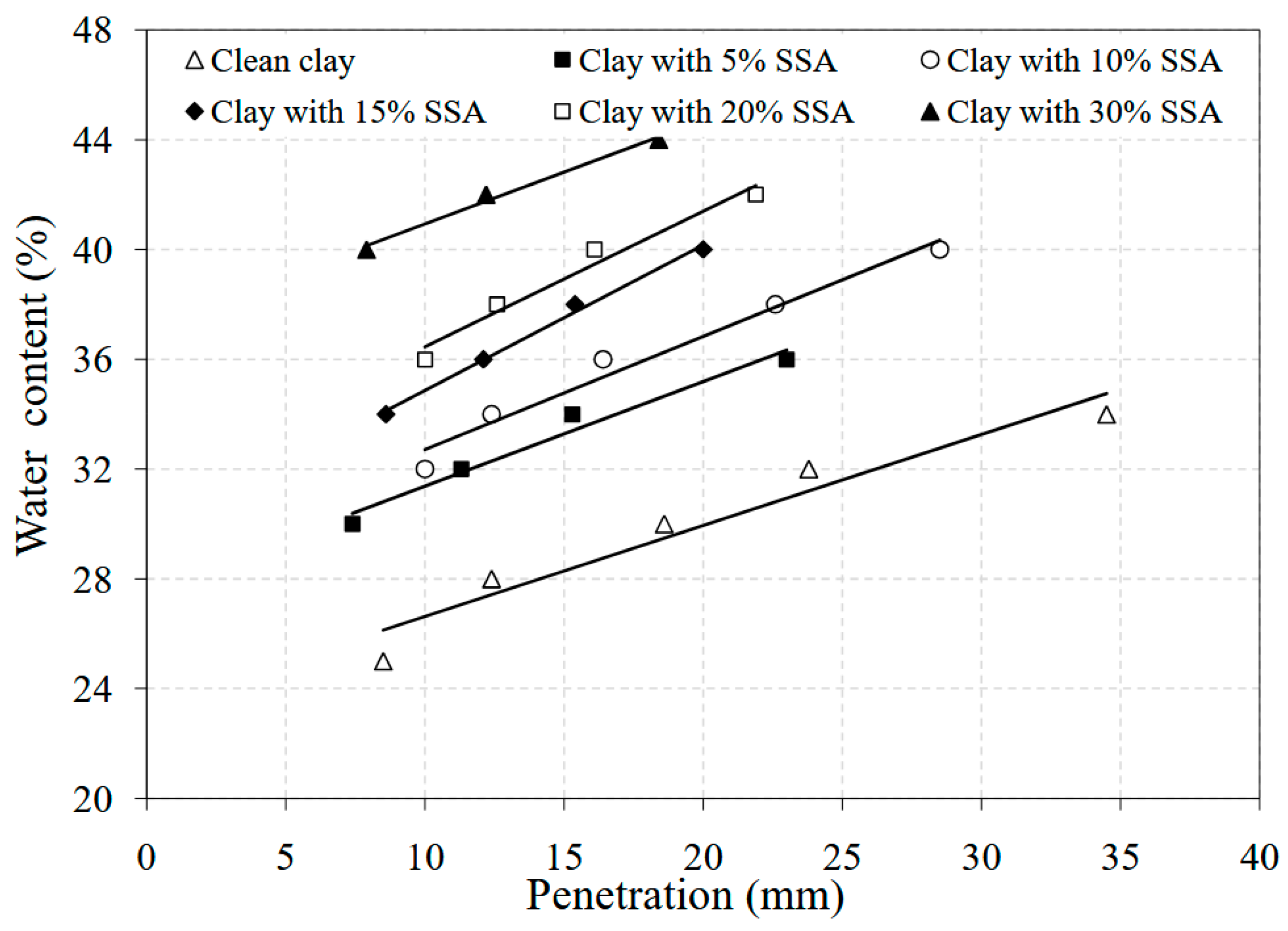
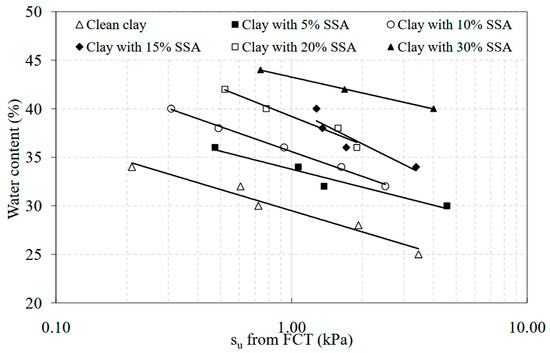
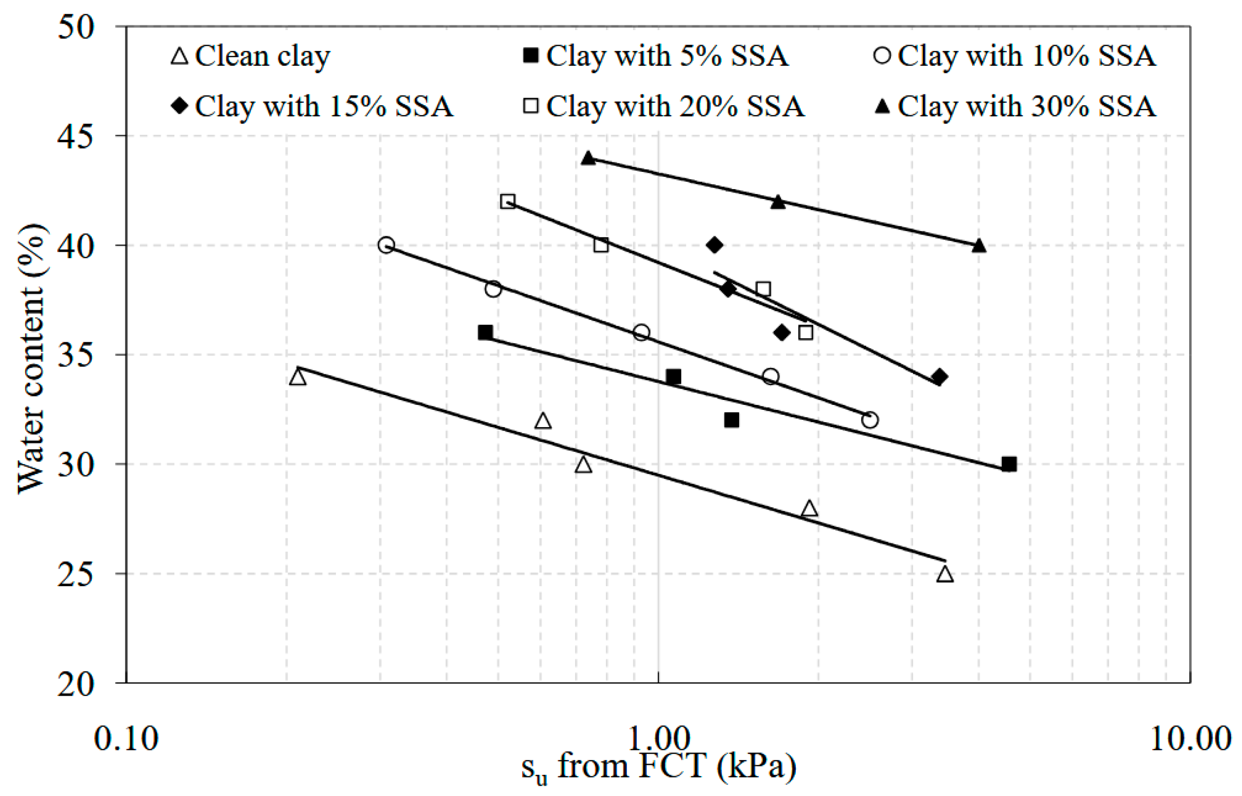
Changes in the fall cone penetration with water content changes for each specimen are presented in Figure 7. As can be seen, there is nearly a linear relationship between the fall cone penetration (mm) and the water content (%). For any water content value in the tested range, penetration values decrease as the amount of SSA in the mixture increases. Based on the fact that the water content corresponding to 20 mm penetration in the fall cone test is the liquid limit [47,48,49], it was clearly observed that the liquid limit values substantially increased. The liquid limit of the clean clay was found to be about 30%, while the clay with 5% SSA, 10% SSA, 15% SSA, 20% SSA, and 30% SSA had liquid limit values of 31%, 34%, 35%, 40%, and 43%, respectively. As can be seen from Figure 8, which presents the change in undrained shear strength (su) with the water content for the specimens tested during the experimental studies, the SSA content in the specimens has a significant effect on the su values obtained from the fall cone tests (FCTs). For example, the su value of the clean CL specimen at about a 35% water content increased from 0.2 kPa to 2.0 kPa with the 10% SSA addition. In the light of the studies by [50,51,52,53], the authors’ interpretation is that the SSA grains behave like a ‘bond’ between the CL grains, rather than a ‘non-plastic fine’ material inside the mixtures tested on the same day. However, the authors theorize that the SSA grains could have a different influence on the behavior of mixtures when the specimens are left for various curing times. Veeresh et al. [54] pointed out that SSA increased the undrained shear strength values. The findings reported by Lin et al. [27] also indicated that SSA increased the triaxial shear strength.
Figure 7.
The effect of the SSA on the cone penetration and water content for the clay–SSA mixtures.
Figure 8.
The effect of the SSA on the su and water content for the clay–SSA mixtures tested in FCTs.
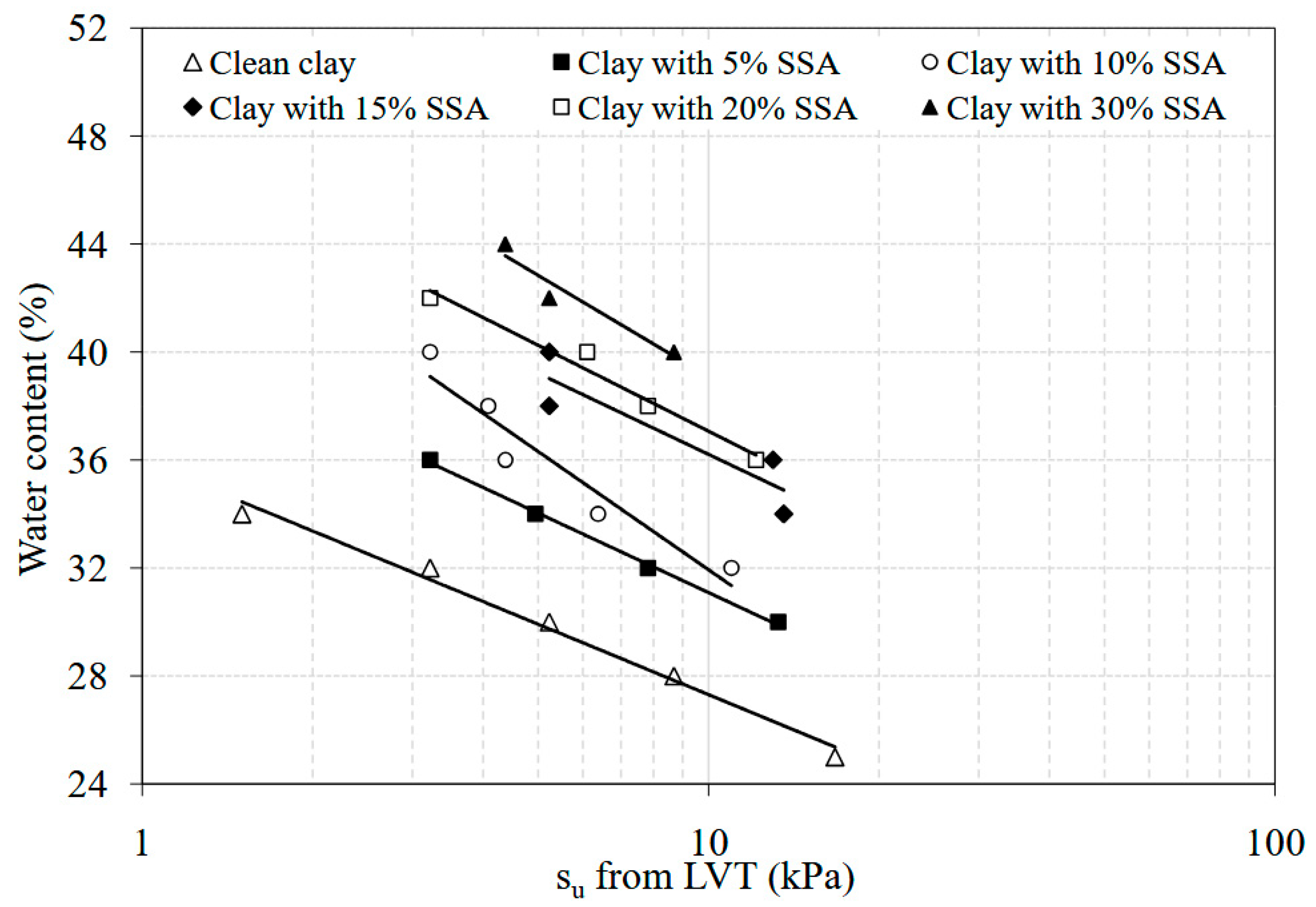
3.4. Effect of SSA on Laboratory Vane Shear Testing Results
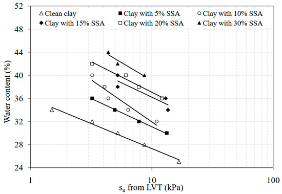
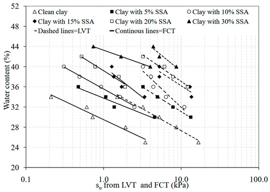
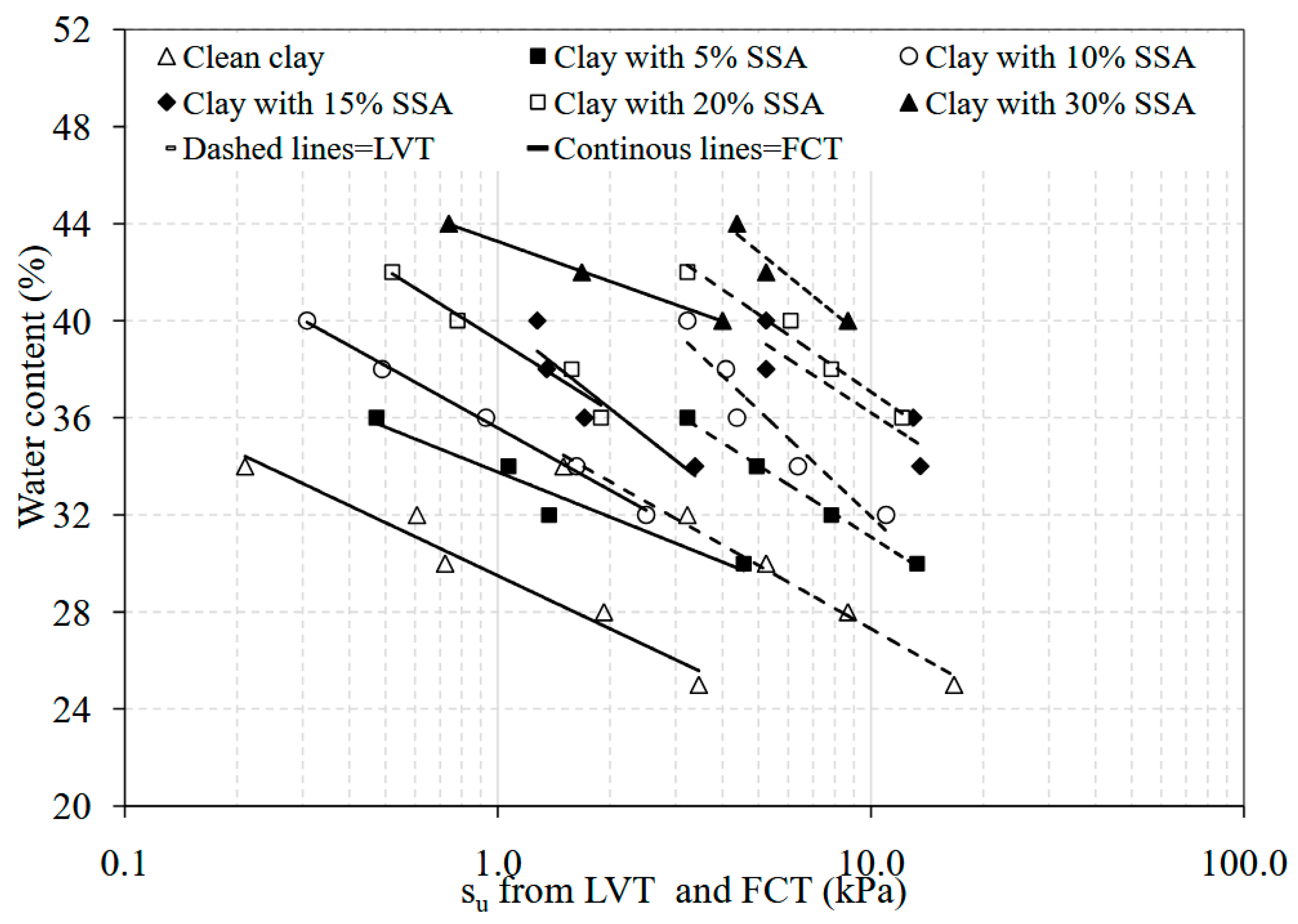
Figure 9 presents the change in su values with water content changes for the specimens tested in laboratory vane shear tests (LVTs). Similarly to the results obtained in fall cone tests, it is observed that as the SSA content in the mixtures increases, the su values increase substantially. A comparative assessment of fall cone and vane shear testing results over the same water content range is provided in Figure 10. The clean clay samples in the LVT results had a su value ranging between 1.7 kPa and 17 kPa, whilst the su values obtained for the same material by the fall cone equipment were found to be from 0.20 kPa to 3.50 kPa for the water contents ranging from 25% to 34%. A similar trend was observed for the clay specimens with SSA additions at various contents. For example, the su values from the fall cone tests on the clay with 30% SSA were observed to be changed from 0.75 kPa to 4.0 kPa, whilst those obtained from LVTs ranged between 4.30 kPa and 8.80 kPa over the water content values ranging from 44% to 40%. The most striking point in Figure 10 is that the su values predicted using the LVT device were much higher than those predicted using the fall cone testing device. Such a difference is likely due to how the testing procedures are defined, what type of vane or cone is used, the rate of rotation adopted, the fall cone roughness, and other intrinsic characteristics [55,56,57].
Figure 9.
The effect of the SSA on the su and water content for the clay–SSA mixtures tested in LVTs.
Figure 10.
Comparing the effect of SSA on the su and water content for the clay–SSA mixtures tested in the FCT and LVT.
3.5. Effect of SSA on Unconfined Compression Strength Testing Results
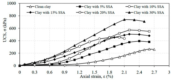
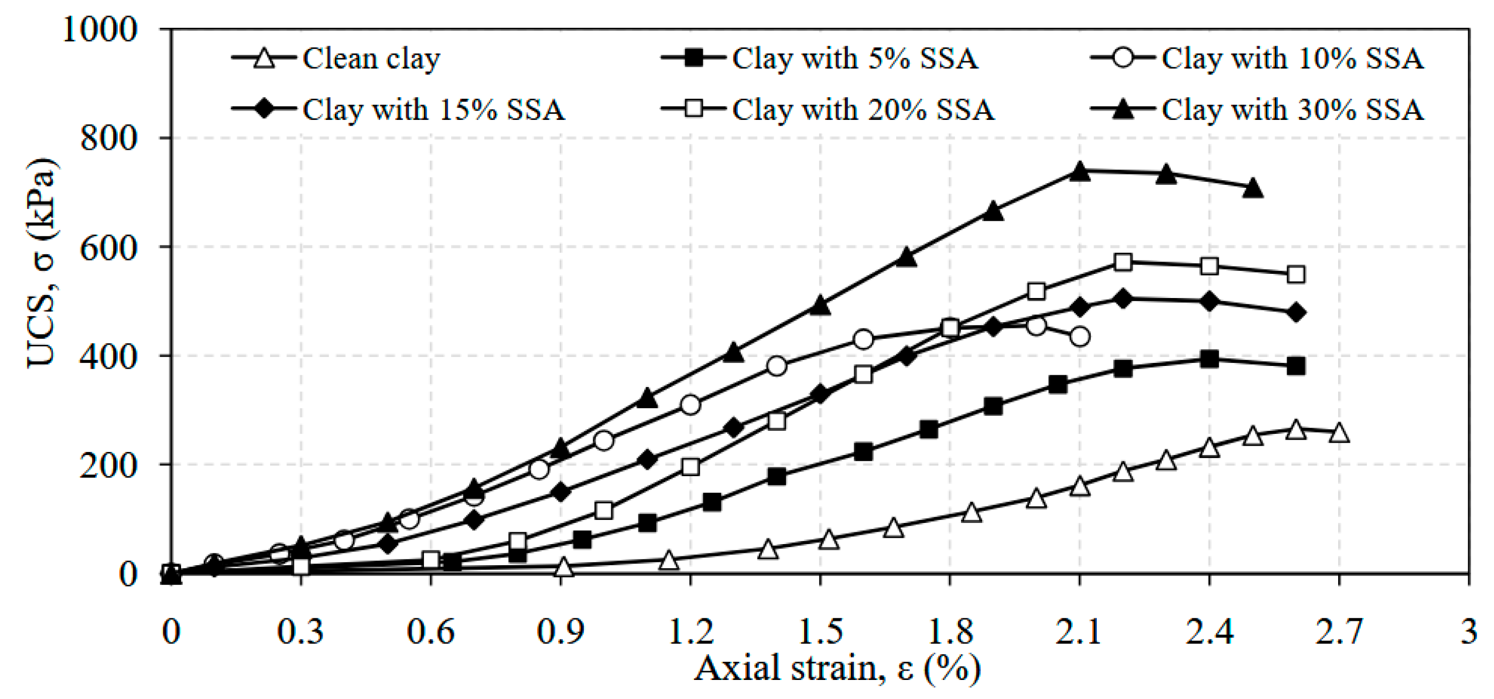
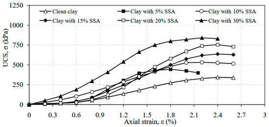
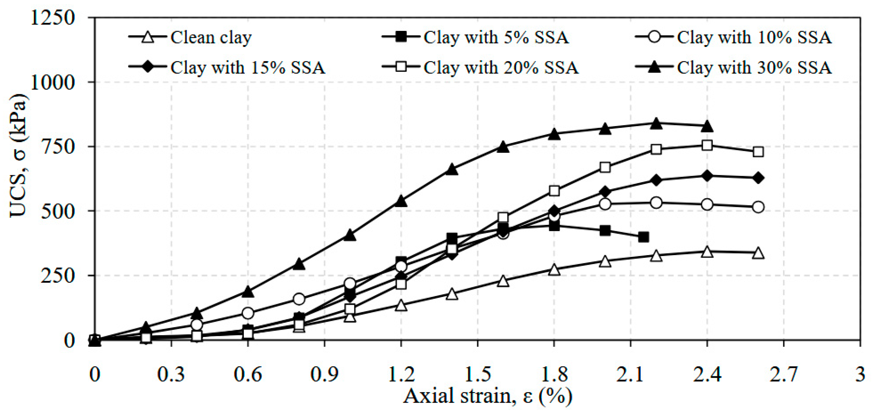
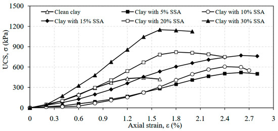
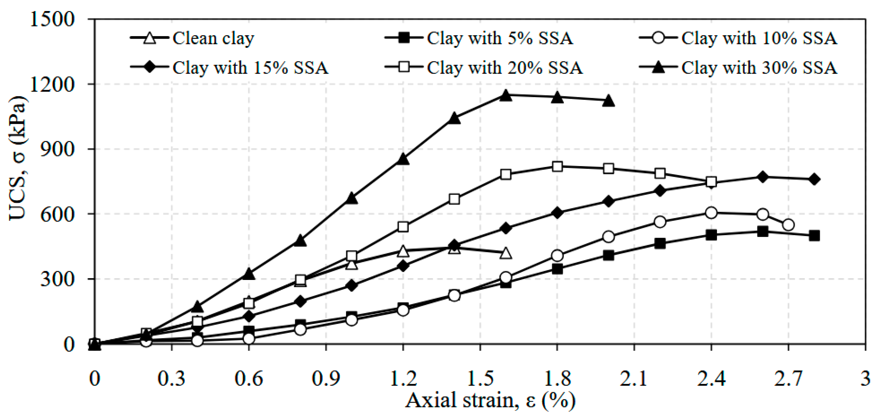
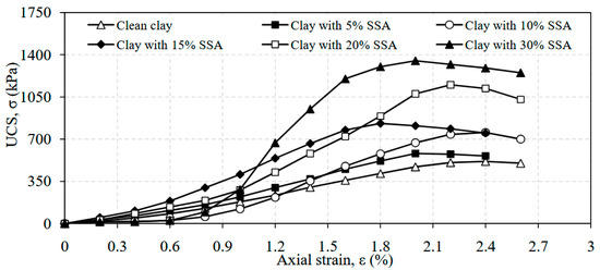
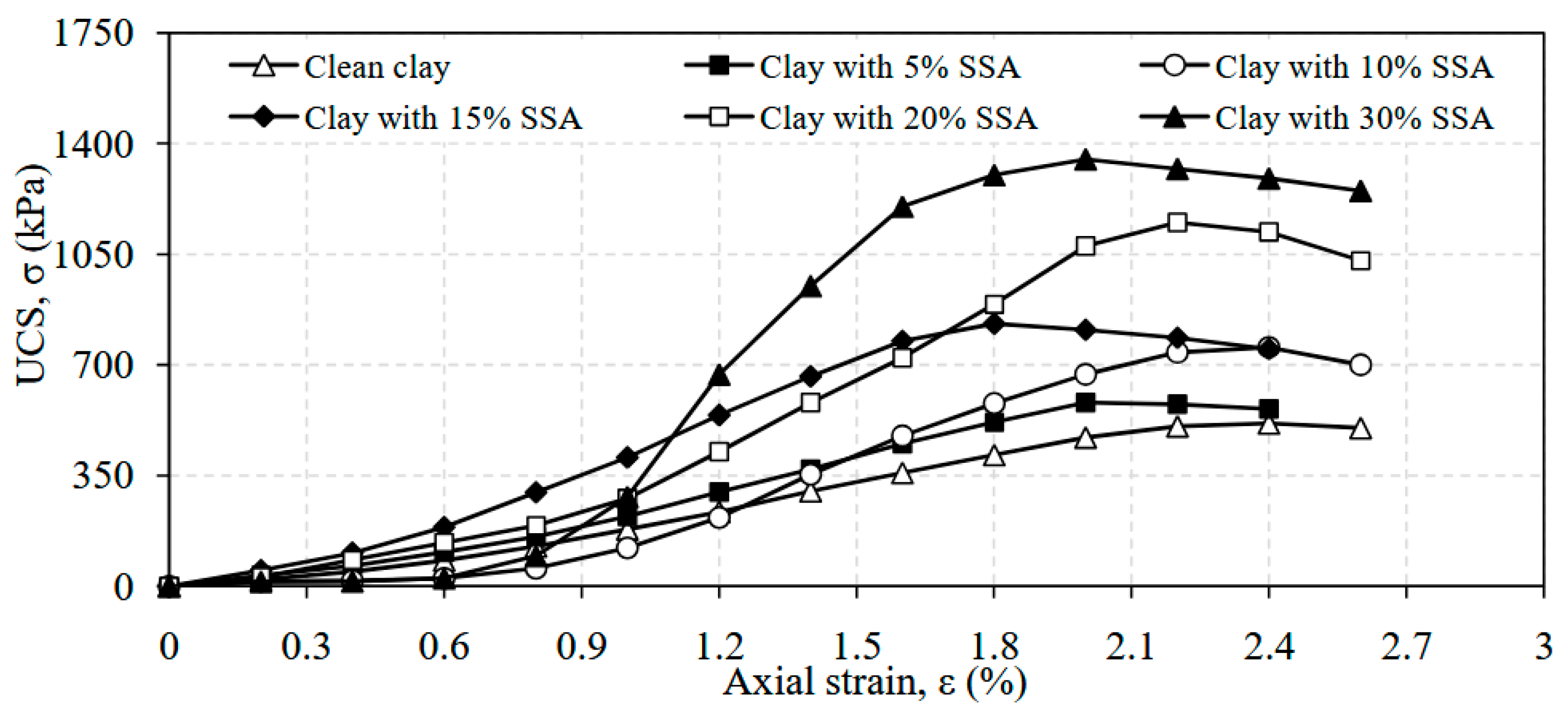
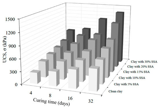
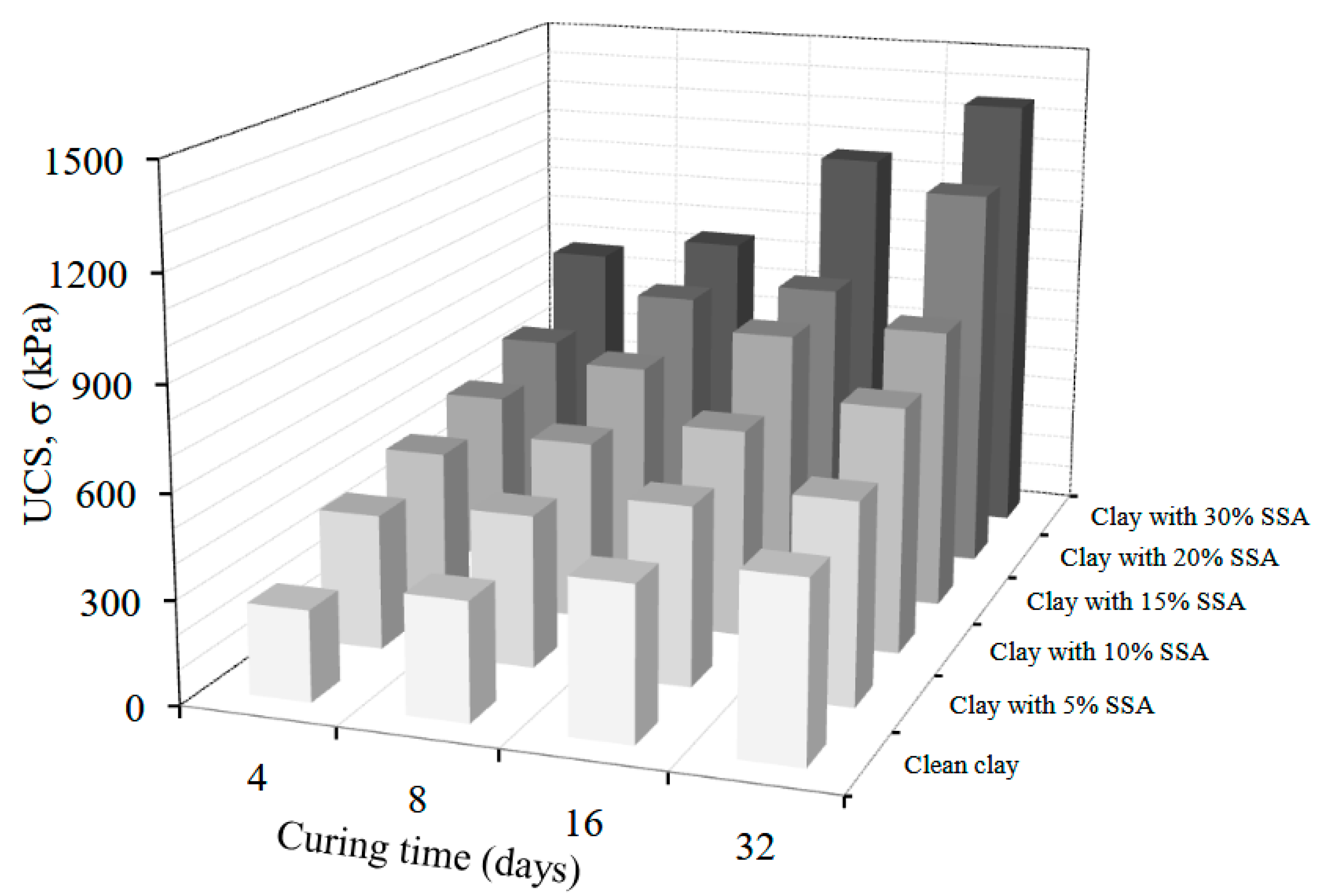
The unconfined compression strength (UCS)testing results were found to be greatly influenced by the addition of SSA. The UCS tests were performed at the optimum water content of each specimen. It is seen that the peak strength values increased substantially as the amount of SSA in the specimens increased. These increments were found to change from 263 kPa to 770 kPa for 4-day-cured-specimens, from 344 kPa to 841 kPa for 8-day-cured-specimens, from 445 kPa to 1150 kPa for 16-day-cured-specimens, and from 514 kPa to 1350 kPa for 32-day-cured-specimens (Figure 11, Figure 12, Figure 13 and Figure 14). A similar trend in many other experimental studies is observed at different levels [29,34,58]. All the test results are presented in a 3-D bar graph for a better understanding of the overall behavior (Figure 15). As can be seen from the Figures, the UCS values have been influenced by curing times and the amount of SSA in the mixtures as well.
Figure 11.
UCS vs. axial strain for 4-day-cured specimens.
Figure 12.
UCS vs. axial strain for 8-day-cured specimens.
Figure 13.
UCS vs. axial strain for 16-day-cured specimens.
Figure 14.
UCS vs. axial strain for 32-day-cured specimens.
Figure 15.
Variation in the maximum UCS values with varying SSA contents and curing times.
Strength gains in SSA–clay mixtures can be largely explained by the SSA’s high CaO, SO3, and P2O5 contents, which promote short-term cation exchange, flocculation, and particle packing in the large size grains (clay: 83%, SSA: 95%). Incorporating such analyses alongside the literature on geopolymer stabilization mechanisms—e.g., ‘Modulation of initial CaO/Al2O3 and SiO2/Al2O3 ratios on the properties of slag/fly ash-based geopolymer stabilized clay’ [59] and ‘Strength behavior and microscopic mechanisms of geopolymer-stabilized waste clays considering clay mineralogy’ [60]—would strengthen the interpretation of the SSA-driven stabilization.
4. Machine Learning Models
Histograms, scatter plots, and unseen dependencies at higher dimensions are part of the ‘ground truths’, and they are as real as physical features such as soil layers [61]. In practice, it is common for sites to be clustered in a ‘region’, whether a geographical area or a geological region. Data-driven clustering can produce solutions outside these traditional geographical/geological limitations [62]. Laboratory test results for natural soils indicate that most soil properties can be considered as random variables conforming to the normal distribution function [63,64]. The spatial variation in soil properties consists of several components and can be represented by a simple model:
This definition of the collective variation in soil properties consists of deterministic and random components and measurement errors [65]. Geotechnical parameters are used to describe the probability distributions and statistical analysis [66]. However, these methods are now at the cusp of transitioning to machine learning methods that are expected to have a profound and wide-ranging impact on the future of geotechnical engineering under the ‘data-first practice-centered’ agenda of data-centric geotechnics [61]. Data processing and software tools have been used to solve many different problems of geotechnical engineering. Deep learning, machine learning, and various data processing methods are used for predicting deformations of deep excavations [67], analyzing liquefaction problems [68,69], predicting and classifying geotechnical parameters [70] and slope stability problems [71,72], determining the strength properties of composite soil environments [73,74,75,76] and site response problems [77], and solving many other problems.
In line with this data-centric perspective, the present study employs machine learning techniques as supportive analytical tools to explore relationships within the experimental dataset and to assist in the interpretation of key geotechnical parameters. Self-Organizing Maps (SOMs) and Support Vector Machines (SVMs) were adopted as complementary, exploratory tools to analyze the experimental dataset. SOMs were used for unsupervised clustering and visualization to identify patterns and relationships among variables, while SVMs were selected for a supervised analysis due to their suitability for small datasets and nonlinear problems. Model parameters were kept simple, and the validation was performed using data partitioning rather than a rigorous cross-validation because of the limited number of samples. Consequently, the numerical results were interpreted as indicative trends rather than fully predictive outcomes, and future studies with larger datasets and more robust validation frameworks are recommended.
A dataset was developed with the results obtained from the experimental studies carried out here. The dataset was processed using Support Vector Machines (SVMs), which are powerful machine learning algorithms used specifically for classification and regression problems. They was first developed by Cortes and Vapnik [78] and are mainly used to classify data points or make predictions in a regression problem. SVMs, when used for classification, attempt to determine a decision boundary that best separates examples belonging to different classes. By dividing the dataset into sections, overfitting problems can be prevented. The accuracy of the model is computed using the observations in the validation fold, and predictions are based on these observations. Most of the design methodologies in geotechnics consider the shear strength of soils as input parameters. Therefore, shear strength parameters deserve the primarily recognition of uncertainty [66]. The undrained shear strength (su), in this set of analyses, is selected as the target parameter, and the curing period, compression strength, maximum dry unit, SSA, and optimum water content were used as input parameters. Two individual analyses were performed with the same input parameters for each target parameter of the undrained shear strength measured by laboratory vane shear tests (LVTs) and fall cone tests (FCTs). Before having the SVM models classify the parameters, a neural-network-based classification approach was attempted to realize the relationship between the parameters. With this classification method, Self-Organizing Maps (SOMs) with a grid size of 8 × 8 neurons were created. SOMs are particularly useful for clustering and visualizing high-dimensional data in lower dimensions while preserving the topological relationships present in the original data. A typical SOM network consists of input layers, interconnection weights, and an output layer with neurons. The SOM clustering technique has recently been used in classification applications in engineering. Klose (2006) [79] classified geophysical data and developed SOM interpretations based on feature clusters. The geotechnical properties of sedimentary soils are clustered with SOMs in a region [80]. SOMs were collectively used with the fuzzy clustering method to evaluate the data of underground projects.
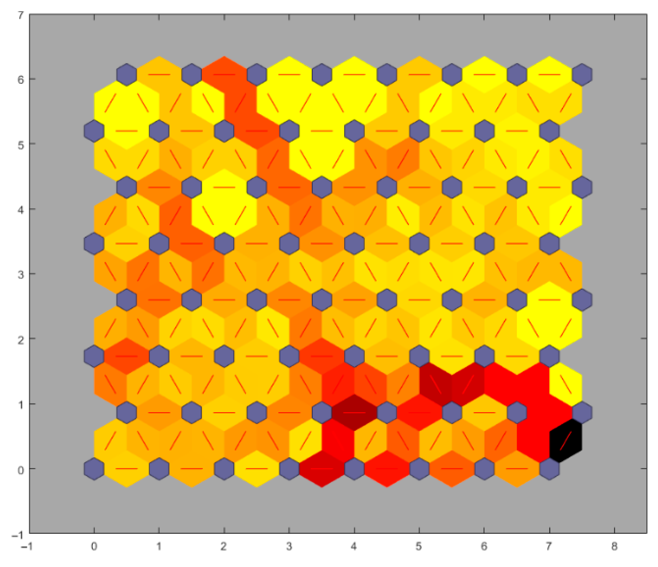
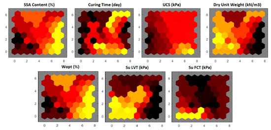
In this study, to conduct a preliminary evaluation of the relations between the parameters, the maps of the training phase of the model are presented in Figure 16. The figure depicting SOM neighbor distances provides insights into the organization and topology preservation of the map during the training process. Each neuron in the SOM grid is associated with a weight vector. The neighbor distances represent the distances between the weight vectors of neighboring neurons in the SOM. These distances help visualize how well the SOM preserves the topology of the input space. Smaller neighbor distances generally indicate a better-organized SOM with more accurate representations of the input data. A well-organized SOM is expected to have shorter neighbor distances between adjacent neurons, leading to a smoother transition in the response of neurons to different input patterns. In this regard, a uniform distribution is observed between the parameters in terms of neighboring weight distances, and local blocks are observed on the global map.
Figure 16.
Neighbor weight distances of the SOMs.
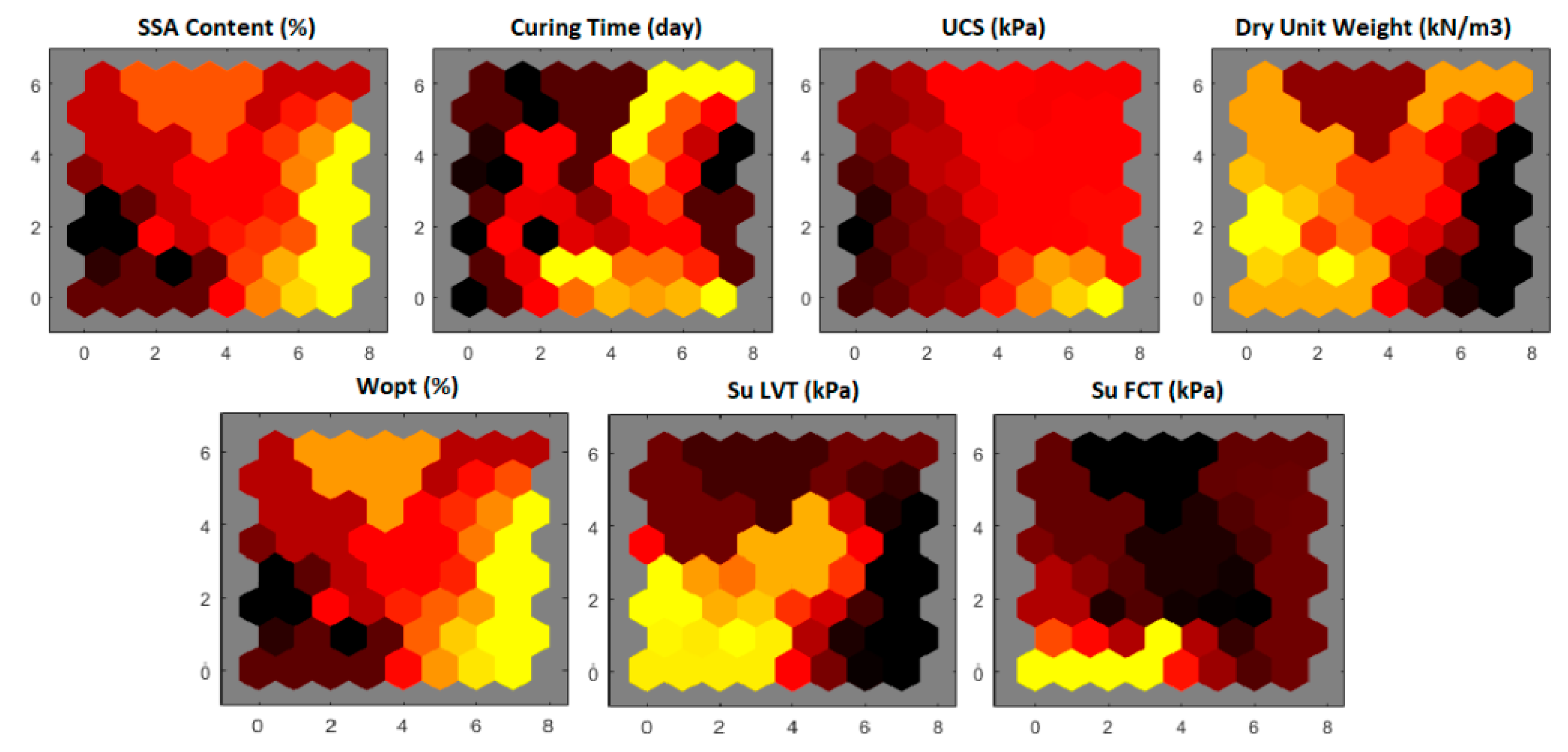
For SOM modeling, 24 datasets, with the main parameters being the SSA content, wopt, curing period, su-LVT, su-FCT, UCS, and dry unit weight values, were used, and the modeling process was conducted in a software environment. Multiple visualizations consisting of hexagonal grids are demonstrated. They show that in the dataset with a length of 24 lines, certain parameters scatter in a wide range within themselves, which is quite suitable for clustering. The SSA content in the hexagonal grid distribution is quite regular as it contains knowledge of six distinct SSA contents (0 to 30%). Colors are often used to identify different clusters or groups of neurons on the SOM grid. Similar or related neurons might be assigned similar colors, helping to visually group them together. Therefore, a color gradient is used to indicate increasing or decreasing values of parameters. The SSA content from 0% to 30% represents a chronological order, which appears to have a similar clustering pattern with wopt in this respect. The UCS of specimens vary between 263 kPa and 1350 kPa within the dataset. A transient relationship is observed within the clusters in the visual representation, where dark colors correspond to low values, and light colors correspond to high values. In this respect, the use of a gradient color scale helps visualize and interpret the information encoded by the SOM in a more intuitive and accessible way. Gaussian neighborhood functions were used in the analysis. In fact, the adopted methodology aims for cluster detection and to discover the relations for data visualization. However, since the dry unit volume weight varies within a very limited range, the ability to visualize a complex model appears to be low. Su-LVT and Su-FCT are two parameters that were set as targets in the SVM analysis. The clustering pattern of both parameters consists of regionally concentrated very low and very high values (Figure 17).
Figure 17.
The SOM clustering results based on the soil characteristics.
The concepts of true positive rates (TPRs) and false negative rates (FNRs) are related to the model’s performance in binary classification tasks. The true positive rate (TPR), also known as sensitivity or recall, measures the proportion of actual positive cases that are correctly identified by the model. It is calculated as follows:
where TPs (true positives) are the number of correctly predicted positive cases, and FNs (false negatives) are the number of positive cases incorrectly classified as negative. A high TPR indicates that the model is effectively capturing a large portion of the positive cases. The false negative rate (FNR) represents the proportion of actual positive cases that are incorrectly classified as negative:
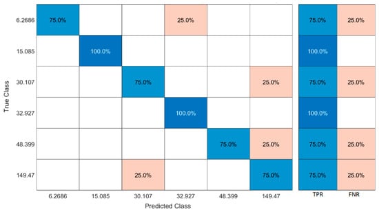
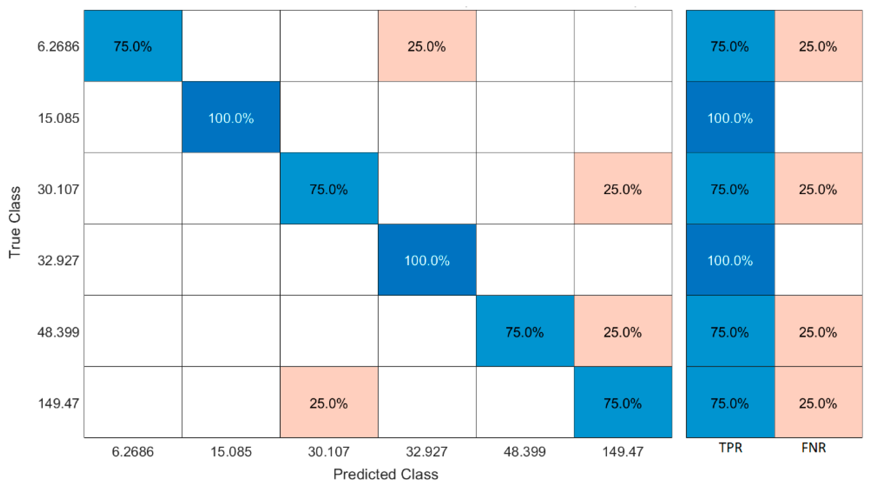
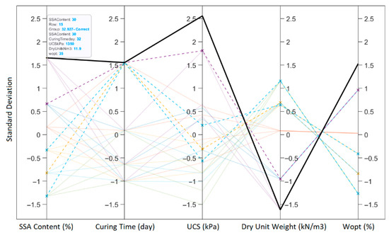
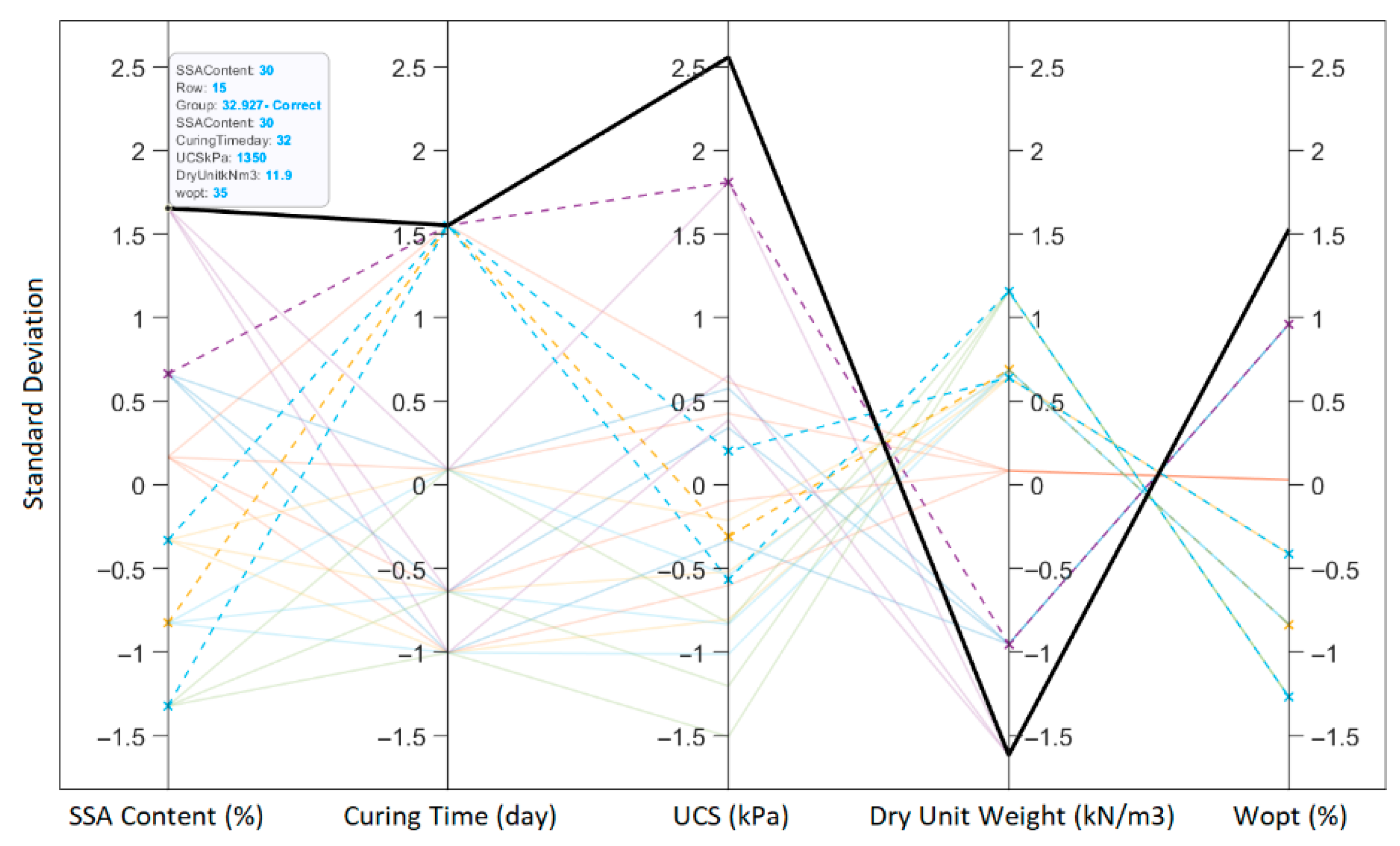
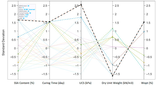
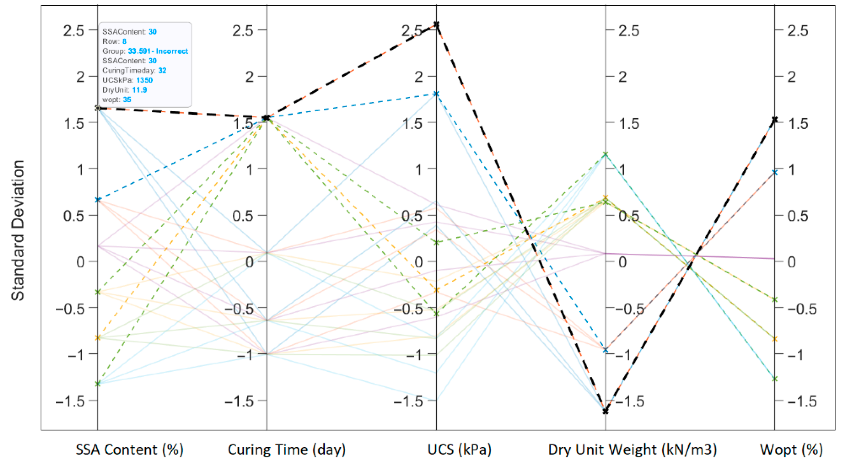
The FNR is the complement of the TPR and measures the model’s failure to identify positive cases. A low FNR is desired, indicating fewer missed positive cases. In SVMs, balancing the TPR and FNR depends on the specific problems. In geotechnical engineering practices, a high TPR (a low FNR) is typically more critical to avoid missing positive cases, even if it means a slightly higher false positive rate. As can be seen in Figure 18, the prediction capacity of the model for the presented dataset is at the highest level for the curing period and dry unit weight of the specimens. Each numeral on the x and y axis of the chart represents the true and predicted values of the su-FCT. For instance, the 75% prediction accuracy means that 75% of the predictions produced by the model for su, which was 6.26 kPa, were correct, and 25% were incorrect, which was 32.927 kPa. Again, it was observed that the su-LVT values in the data sets of 15.085 kPa and 32.927 kPa were predicted with strong accuracy. At the end of these predictions for each su-LVT value, the cumulative prediction success of the SVM model was calculated as 83.33%, which is a very satisfactory level. This high level of success for a very limited dataset indicates an impressive performance for comprehensive geotechnical laboratory work programs. In addition, the dynamic variation in each input parameter throughout the analysis and the standard deviation calculated for each prediction are shown on the parallel coordinate graphic plane (Figure 19).
Figure 18.
The confusion matrix developed for the su obtained by the FCT.
Figure 19.
Parallel coordinates of input parameters in the medium Gaussian SVM developed for the su obtained by the FCT.
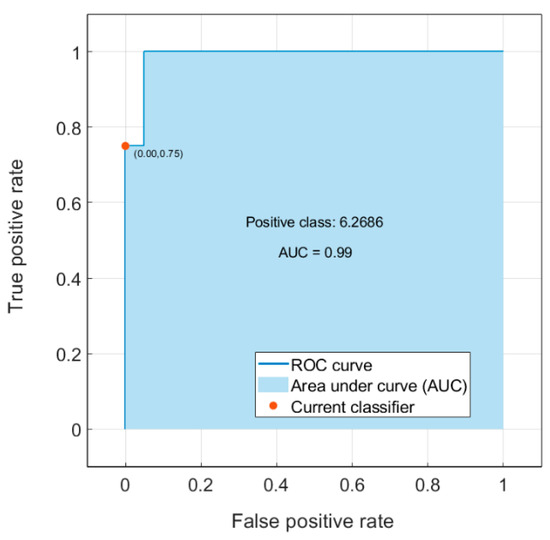
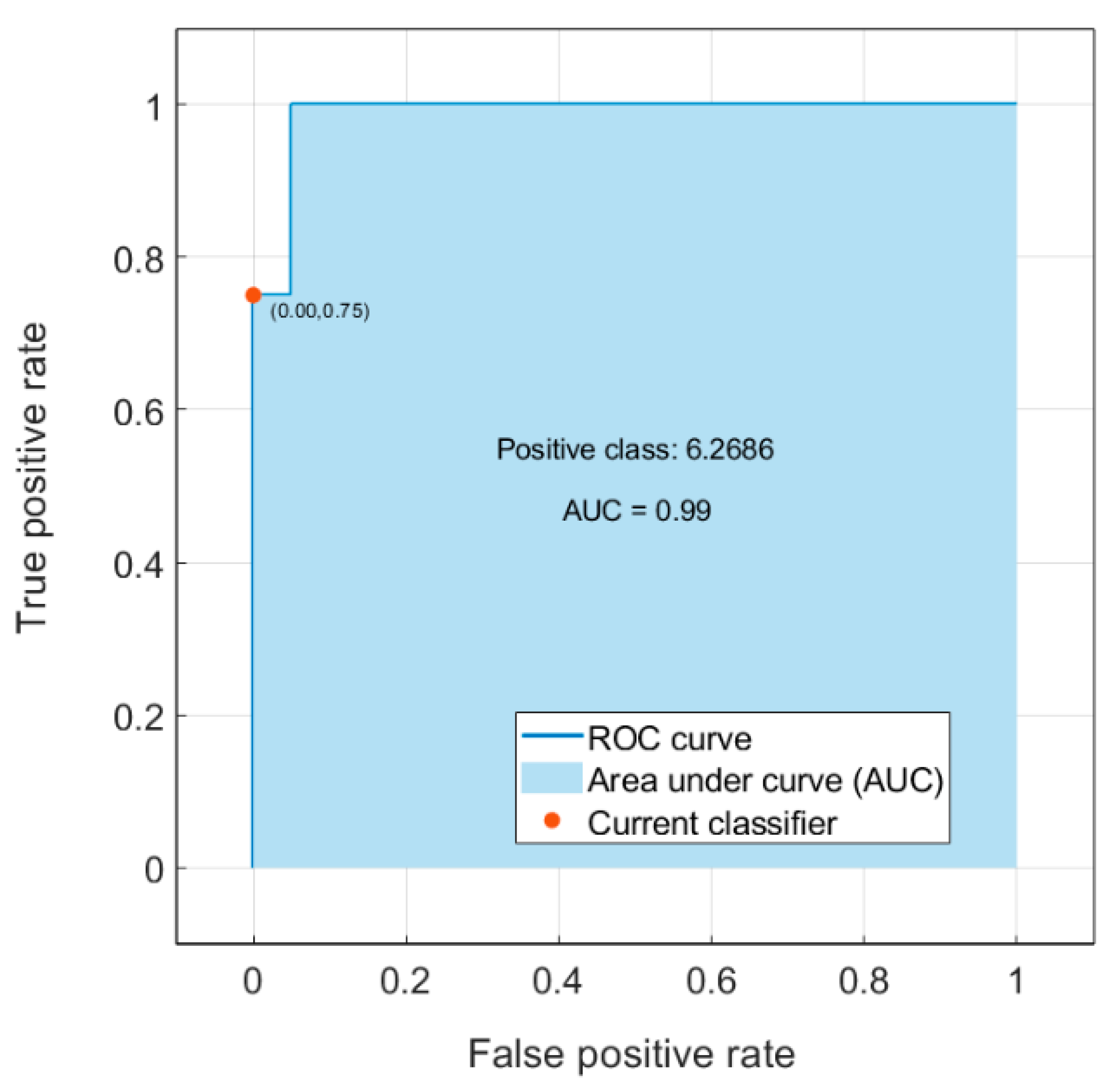
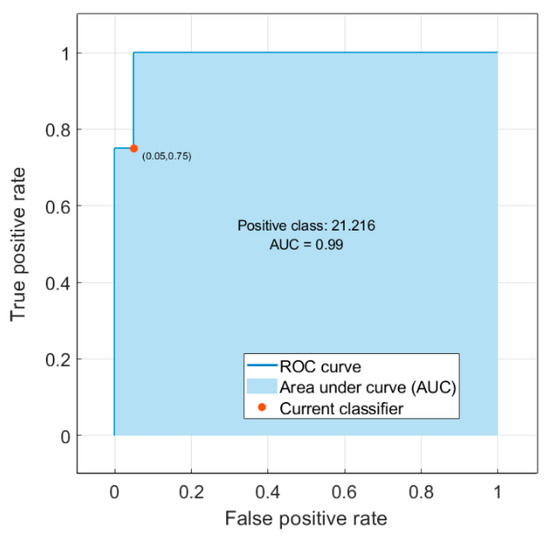
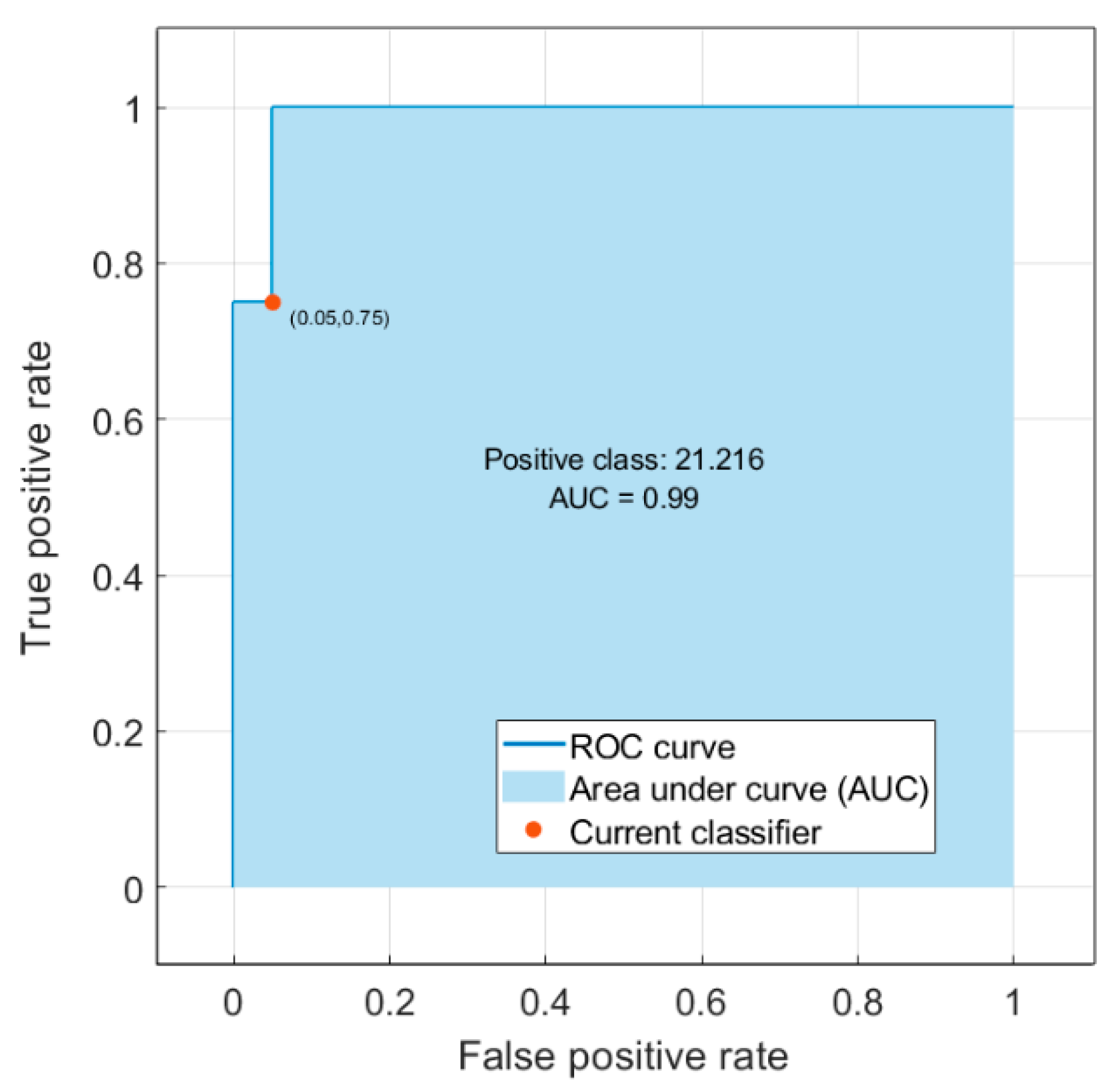
The Receiver Operating Characteristic (ROC) curve and Area Under the Curve (AUC) are tools used to evaluate and compare the performance of machine learning classifiers, especially in binary classification problems. An ROC curve is a graphical representation that illustrates the performance of a binary classifier at various threshold settings. It plots the true positive rate (sensitivity/recall) against the false positive rate (1—specificity) for different threshold values. The true positive rate (TPR), as previously formulated, is the ratio of correctly predicted positive observations to the total actual positives. The false positive rate (FPR) is the ratio of incorrectly predicted negatives to the total actual negatives. In an ROC curve, the x-axis represents the FPR, and the y-axis represents the TPR. A diagonal line (representing random guessing) is the baseline, and a good classifier will have its curve above this line, indicating a better-than-random performance. The AUC quantifies the overall performance of a classifier. It represents the area under the ROC curve. A perfect classifier would have an AUC of 1, indicating that it achieves a TPR of 1 (100% true positives) without any false positives (FPR of 0). A completely random classifier would have an AUC of 0.5, corresponding to the diagonal line. In this case, a very high AUC value (i.e., 0.99) implies a high ability of the classifier across various threshold settings. Interpreting the AUC and the shape of the ROC curve helps for assessing the classifier’s performance without being influenced by a specific decision threshold. In this classification study, where the curve shows a very stable behavior, it is clearly seen that it does not change its behavior at any threshold level, which is compatible with the prediction success of the model. This is undoubtedly related to the quality of the dataset used (Figure 20).
Figure 20.
The ROC curve of the predictive model for the validation of the su obtained by the FCT.
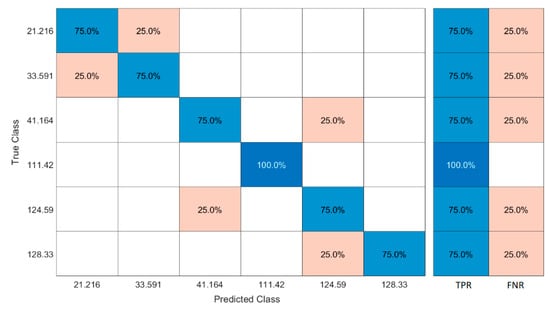
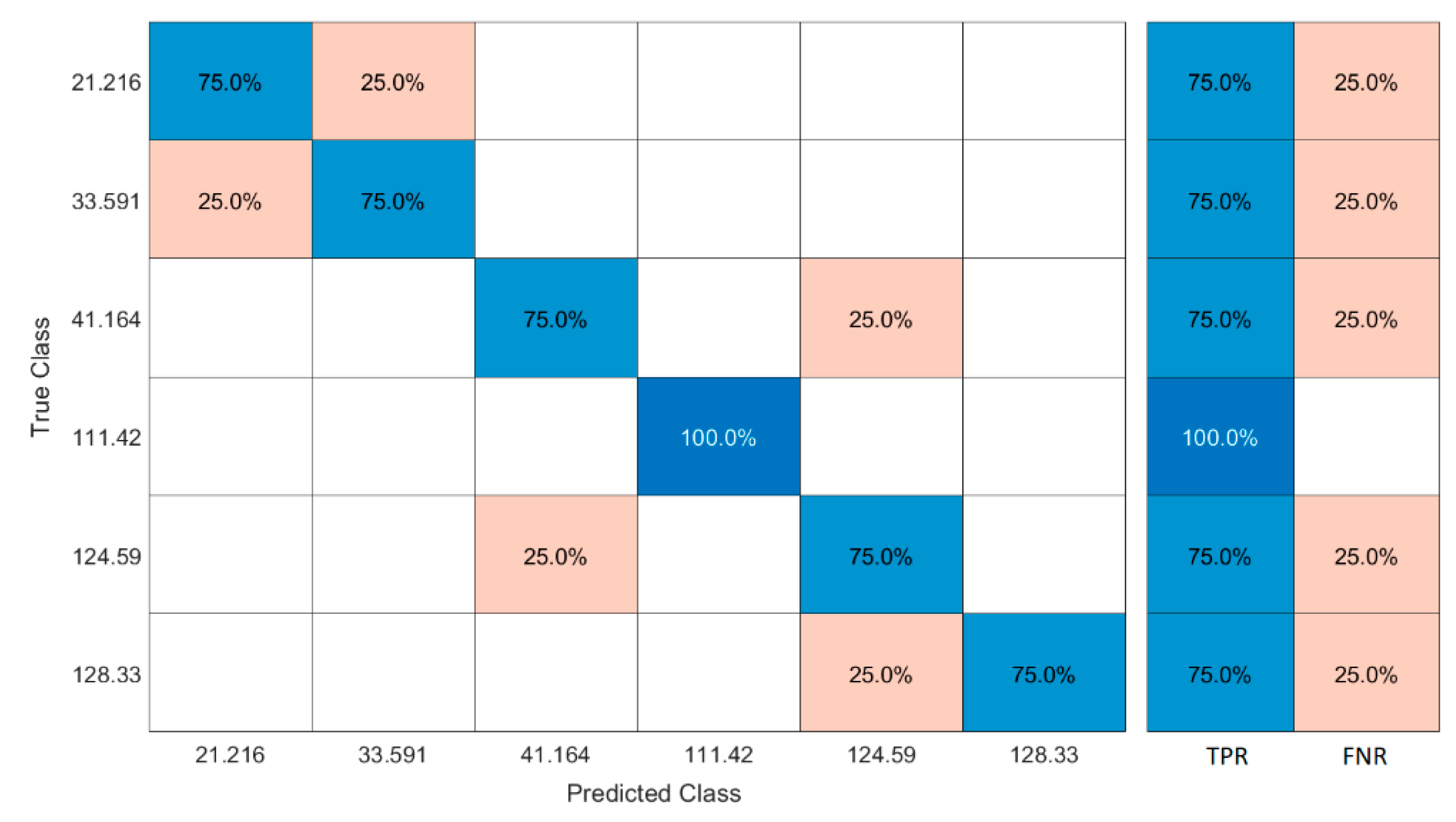
Similar analyses were carried out for the su-LVT target parameter. An SVM classification learning study was carried out with a slightly lower accuracy level than the previous analysis results. It is seen that the model produced a fully accurate prediction for the dataset where the su value was 111.42 kPa, but the prediction success decreased to 79.2% for the datasets containing remaining su-LVT values (Figure 21). It is seen that the standard deviation achieves the highest value in response to the change in the UCS parameter (Figure 22). On the other hand, the curing time parameter stands out as the parameter that causes the least deviation, as expected, like the previous model. The reason for this is that the variability of the curing time parameter is low. The AUC value was again quite high, confirming the model’s classification success (Figure 23).
Figure 21.
The confusion matrix developed for the su obtained by the LVT.
Figure 22.
Parallel coordinates of input parameters of the medium Gaussian SVM developed for the su obtained by the LVT.
Figure 23.
The ROC curve of the predictive model for the validation of the su-LVT.
5. Conclusions
This study aimed to investigate the effect of SSA on some characteristics of a CL-type clay. An intensive series of laboratory tests have been carried out on the specimens of clay and SSA at different ratios (0%, 5%, 10%, 15%, 20%, and 30% by dry weight). The tests reported in this research point out six new facets of behavior:
- From the Atterberg results, the classifications of the specimens tested have been changed from an inorganic clay with low plasticity (CL) to inorganic silt with low plasticity (ML) by adding SSA grains, in accordance with the unified soil classification system (USCS).
- The maximum dry density of the specimens decreased as the amount of SSA increased. Also, the sensitivity of the mixture to water decreased with the addition of SSA grains.
- Penetration values in the fall cone tests decreased as the amount of SSA in the mixture increased.
- The su values obtained in the laboratory vane shear tests increased as the SSA content in the mixtures increased.
- The su values predicted using the laboratory vane shear testing device were found to be higher than those predicted using the fall cone testing device.
- The peak UCS values increased substantially as the amount of SSA in the specimens increased.
These experimental findings suggest that in the specimen formation method used here, the SSA grains behave like a ‘bond’ between the CL grains, rather than a ‘non-plastic fine’ material inside the specimens tested. Furthermore, the classification and prediction of the parameters in the dataset were carried out using SOMs and SVMs (unsupervised and supervised learning algorithms, respectively), two neural-network-based computing methods. The su-LVT and su-FCT results were predicted with very high validation accuracies of 83.3% and 79.2%. The fact that both methods were employed in the same study as geotechnical data-based algorithms and exhibited satisfactory performances formed the basis for a unique approach. We aimed to evaluate the results of labor-intensive experimental studies using innovative methods as an example of multidisciplinary approach models. The machine learning analyses presented in this study are exploratory and intended to support the interpretation of the experimental results. Given the limited dataset and the lack of rigorous cross-validation, these methods should not be regarded as predictive tools. Their outcomes are therefore reported as indicative trends only. The long-term durability, environmental performance (e.g., leaching behavior), and field-scale validation were also beyond the scope of the present study. Future research should address these aspects to further substantiate the applicability of SSA as a sustainable soil stabilization agent.
Author Contributions
Conceptualization, A.F.C.; Software, O.Y.; Investigation, N.A.; Writing—original draft, N.A.; Writing—review & editing, A.F.C.; Supervision, A.F.C. All authors have read and agreed to the published version of the manuscript.
Funding
This research received no specific grant from any funding agency in the public, commercial, or not-for-profit sectors.
Institutional Review Board Statement
Not applicable.
Informed Consent Statement
Not applicable.
Data Availability Statement
The datasets generated and analyzed during the current study are available from the corresponding author on reasonable request.
Conflicts of Interest
The authors declare that they have no known competing financial interests or personal relationships that could have appeared to influence the work reported in this paper.
References
- Lundin, M.; Olofsson, M.; Pettersson, G.J.; Zetterlund, H. Environmental and economic assessment of sewage sludge handling options. Resour. Conserv. Recycl. 2004, 41, 255–278. [Google Scholar] [CrossRef] [Scilit]
- Ravindra, K.; Kaur, K.; Mor, S. System analysis of municipal solid waste management in Chandigarh and minimization practices for cleaner emissions. J. Clean. Prod. 2015, 89, 251–256. [Google Scholar] [CrossRef] [Scilit]
- Dhir, R.K.; Ghataora, G.S.; Lynn, C.J. Sustainable Construction Materials; Chapter 4: Sewage Sludge Ash Characteristics; Woodhead Publishing: Sawston, UK, 2017; pp. 69–110. ISBN 978-0081009871. [Google Scholar]
- Tay, J.H.; Show, K.Y. Municipal wastewater sludge as cementitious and blended cement materials. J. Cem. Concr. Compos. 1994, 16, 39–48. [Google Scholar] [CrossRef] [Scilit]
- Anderson, M.; Skerratt, R.G.; Thomas, J.P.; Clay, S.D. Case study involving using fluidized bed Incinerator sludge ash as a partial clay substitute in brick manufacture. Wat. Sci. Technol. 1996, 34, 3–4. [Google Scholar] [CrossRef] [Scilit]
- Lin, D.F.; Weng, C.H. Use of sewage sludge ash as brick material. J. Environ. Eng. 2001, 127, 922–927. [Google Scholar] [CrossRef] [Scilit]
- Brar, G.; Giamouridis, D.; Liodakis, M. Predicting European take over targets. Eur. Financ. Manag. 2009, 15, 430–450. [Google Scholar] [CrossRef] [Scilit]
- Johnson, O.A.; Napiah, M.; Kamaruddin, I. Potential uses of Waste Sludge in Construction Industry: A Review. J. Appl. Sci. Eng. Technol. 2014, 8, 565–570. [Google Scholar] [CrossRef] [Scilit]
- Lynn, C.J.; Dhir, R.K.; Ghataora, G.S. Sewage sludge ash characteristics and potential for use in bricks, tiles and glass ceramics. Water Sci. Technol. 2016, 74, 17–29. [Google Scholar] [CrossRef] [Scilit] [PubMed]
- Li, J.-S.; Guo, M.-Z.; Xue, Q.; Poon, C.S. Recycling of incinerated sewage sludge ash and cathode ray tube funnel glass in cement mortars. J. Clean. Prod. 2017, 152, 142–149. [Google Scholar] [CrossRef] [Scilit]
- Bahadori, H.; Hosseini, P. Developing green cement paste using binary and ternary cementitious blends of low pozzolanic sewage sludge ash and colloidal nanosilica (short-term properties). Asian J. Civ. Eng. 2018, 19, 501–511. [Google Scholar] [CrossRef] [Scilit]
- Rosli, N.A.; Azizb, H.A.; Selamatb, M.R.; Lima, L.L.P. A Mixture of Sewage Sludge and Red Gypsum as an Alternative Material for Temporary Landfill Cover. J. Environ. Manag. 2020, 263, 110420. [Google Scholar] [CrossRef] [Scilit] [PubMed]
- Istuque, D.B.; Reig, L.; Soriano, L.; Borrachero, M.V.; Melges, J.L.P.; Akasaki, J.L.; Bernabeu, J.J.P.; Tashima, M.M. Evaluation of the Pozzolanic Activity of Uncontrolled-Combusted Sewage Sludge Ash. J. Mater. Civ. Eng. 2021, 33, 6. [Google Scholar] [CrossRef] [Scilit]
- Donatello, S.; Cheeseman, C.R. Recycling and recovery routes for incinerated sewage sludge ash (ISSA): A review. Waste Manag. 2013, 33, 2328–2340. [Google Scholar] [CrossRef] [Scilit] [PubMed]
- Perez, M.C.; Baeza, F.B.; Paya, J.; Saval, J.M.; Zornoza, E. Potential Use of Sewage Sludge Ash (SSA) as a Cement Replacement in Precast Concrete Blocks. Mater. Constr. 2014, 64, 313. [Google Scholar] [CrossRef] [Scilit]
- Ciaran, J.L.; Ravindra, K.D.; Gurmel, S.G.; Roger, P.W. Sewage Sludge Ash Characteristics and Potential for Use in Concrete. Constr. Build. Mater. 2015, 98, 767–779. [Google Scholar] [CrossRef] [Scilit]
- Dyer, T.D.; Halliday, J.E.; Dhir, R.K. Hydration Chemistry of Sewage Sludge Ash Used as a Cement Component. J. Mater. Civ. Eng. 2011, 23, 648–655. [Google Scholar] [CrossRef] [Scilit]
- Tenza-Abril, A.J.; Saval, J.M.; Cuenca, A. Using sewage sludge ash as filler in bituminous mixes. J. Mater. Civ. Eng. 2014, 27, 1–9. [Google Scholar] [CrossRef] [Scilit]
- Khanbilvardi, R.; Afshari-Tork, S. Sludge ash as fine aggregate for concrete mix. J. Environ. Eng. 1995, 121, 633–638. [Google Scholar] [CrossRef] [Scilit]
- Monzó, J.; Payá, J.; Borrachero, M.V.; Girbés, I. Reuse of sewage sludge ashes (SSA) in cement mixtures: The effect of SSA on the workability of cement mortars. Waste Manag. 2003, 23, 373–381. [Google Scholar] [CrossRef] [Scilit]
- Chen, Z.; Poon, C.S. Comparative studies on the effects of sewage sludge ash and fly ash on cement hydration and properties of cement mortars. Constr. Build. Mater. 2017, 154, 791–803. [Google Scholar] [CrossRef] [Scilit]
- Vouk, D.; Nakic, D.; Stirmer, N.; Cheeseman, C.R. Use of sewage sludge ash in cementitious materials. Rev. Adv. Mater. Sci. 2017, 49, 158–170. [Google Scholar]
- Kappel, A.; Viader, R.P.; Kowalski, K.P. Utilisation of electrodialytically treated sewage sludge ash in mortar. Waste Biomass Valori. 2018, 9, 2503–2515. [Google Scholar] [CrossRef] [Scilit]
- Liang, C.; Le, X.; Fang, W.; Zhao, J.; Fang, L.; Hou, S. The Utilization of Recycled Sewage Sludge Ash as a Supplementary Cementitious Material in Mortar: A Review. Sustainability 2022, 14, 4432. [Google Scholar] [CrossRef] [Scilit]
- Al-Sayed, M.H.; Madany, M.M.; Buali, A.R.M. Use of sewage sludge ash in asphaltic paving mixes in hot regions. Constr. Build. Mater. 1995, 9, 19–23. [Google Scholar] [CrossRef] [Scilit]
- Merino, I.; Arévalo, L.F.; Romero, F. Preparation and characterization of ceramic products by thermal treatment of sewage sludge ashes mixed with different additives. Waste Manag. 2007, 27, 1829–1844. [Google Scholar] [CrossRef] [Scilit]
- Lin, D.F.; Luo, H.L.; Sheen, Y.N. Glazed tiles manufactured from incinerated sludge ash and clay. J. Air Waste Manag. Assoc. 2005, 55, 163–172. [Google Scholar] [CrossRef] [Scilit] [PubMed]
- Al-Sharif, M.; Attom, M.F. A geoenvironmental application of incinerated wastewater sludge ash in soil stabilization. Environ. Earth Sci. 2014, 71, 2453–2463. [Google Scholar] [CrossRef] [Scilit]
- Ingunza, D.; Santos Junior, M.P.O.; Andrade Medeiros, S. Sewage sludge as raw material in asphalt mixtures. Advandce Mater. Res. 2014, 664, 638–643. [Google Scholar] [CrossRef] [Scilit]
- Kadhim, Y.M.; Al-Adhamii, R.A.J.; Fattah, M.Y. Geotechnical properties of clayey soil improved by sewage sludge ash. J. Air Waste Manag. Assoc. 2022, 72, 34–47. [Google Scholar] [CrossRef] [Scilit] [PubMed]
- Zhou, Y.; Lu, J.; Li, J.; Cheeseman, C.; Poon, C.S. Effect of NaCl and MgCl2 on the hydration of lime-pozzolan blend by recycling sewage sludge ash. J. Clean. Prod. 2021, 313, 127759. [Google Scholar] [CrossRef] [Scilit]
- Lim, S.M.; He, L.; Goh, S.H.; Lee, F.H. Strength of Chemically Stabilized Sewage Sludge- Some Inferences from Recent Studies. Geotechnics 2021, 1, 573–587. [Google Scholar] [CrossRef] [Scilit]
- Chen, L.; Lin, D.F. Stabilization treatment of soft subgrade soil by sewage sludge ash and cement. J. Hazard. Mater. 2009, 162, 321–327. [Google Scholar] [CrossRef] [Scilit]
- Tempest, B.Q.; Pando, M.A. Characterization and demonstration of reuse applications of sewage sludge ash. Int. J. Geomat. Geosci. 2013, 4, 552–559. [Google Scholar]
- Norouzian, K.; Abbasi, N.; Abedi Koupai, J. Use of Sewage Sludge Ash and Hydrated Lime to Improve the Engineering Properties of Clayey Soils. Geotech. Geol. Eng. 2018, 36, 1575–1586. [Google Scholar] [CrossRef] [Scilit]
- ASTM D 422-10:2007; Standard Test Method for Particle Size Analysis of Soils. Annual Book of ASTM Standards. ASTM international: Philadelphia, PA, USA, 2007.
- ASTM D 4318-10:2012; Standard Test Methods for Liquid Limit, Plastic Limit, and Plasticity Index of Soils. Annual Book of ASTM Standards. ASTM international: Philadelphia, PA, USA, 2012.
- ASTM D 698-12:2012; Standard Test Methods for Laboratory Compaction Characteristics of Soil Using Standard Effort. ASTM International: West Conshohocken, PA, USA, 2012.
- BS 1377-2:2022; Methods of Test for Soils for Civil Engineering Purposes Classification Tests and Determination of Geotechnical Properties. British Standards Institution: London, UK, 2022.
- ASTM D 4648-08:2008; Standard Test Method for Laboratory Miniature Vane Shear Test for Saturated Fine-Grained Clayey Soil. ASTM International: West Conshohocken, PA, USA, 2008.
- ASTM D 2166-06:2013; Standard Test Method for Unconfined Compressive Strength of Cohesive Soil. ASTM International: West Conshohocken, PA, USA, 2013.
- Wegman, D.E.; Young, D.S. Testing and evaluating sewage sludge ash in asphalt paving mixtures. Presented at the 67th Annual Transportation Research Board Meeting, Washington, DC, USA, 10–14 January 1988. [Google Scholar]
- Merino, I.; Arévalo, L.F.; Romero, F. Characterization and possible uses of ashes form wastewater treatment plants. Waste Manag. 2005, 25, 1046–1054. [Google Scholar] [CrossRef] [Scilit]
- Yusuf, R.O.; Noor, Z.Z.; Din, M.F.M.; Abba, A.H. Use of sewage sludge ash (SSA) in the production of cement and concrete–A review. Int. J. Glob. Environ. Issues 2012, 12, 214–228. [Google Scholar] [CrossRef] [Scilit]
- Sato, Y.; Oyamada, T.; Hanehara, S.; Sasaki, T. The characteristics of ash of sewage sludge (SSA) in Iwate prefecture and application of SSA for asphalt mixture. J. Min. Mater. Process. Inst. Jpn. 2012, 128, 519–525. [Google Scholar] [CrossRef] [Scilit]
- Deng, F.L.; Kae, L.L.; Huan, L.L. A Comparison between Sludge Ash and Fly Ash on the Improvement in Soft Soil. J. Air Waste Manag. Assoc. 2016, 57, 59–64. [Google Scholar] [CrossRef] [Scilit]
- Feng, T.W. A linear log d log w model for the determination of consistency limits of soils. Can. Geotech. J. 2001, 38, 1335–1342. [Google Scholar] [CrossRef] [Scilit] [PubMed]
- Likos, W.J.; Jaafar, R. Laboratory fall cone testing of unsaturated sand. J. Geotech. Geoenviron. Eng. 2014, 140, 7. [Google Scholar] [CrossRef] [Scilit]
- Cabalar, A.F.; Demir, S. Fall-cone testing of unsaturated sand–clay mixtures. Proc. Inst. Civ. Eng.-Geotech. Eng. 2019, 172, 432–441. [Google Scholar] [CrossRef] [Scilit]
- Thevanayagam, S. Effect of fines on confining stress on undrained shear strength of silty sands. J. Geotechnnical Geoenviron. Eng. 1998, 124, 479–491. [Google Scholar] [CrossRef] [Scilit]
- Monkul, M.M.; Ozden, G. Compressional behavior of clayey sand and transition fines content. Eng. Geol. 2007, 89, 195–205. [Google Scholar] [CrossRef] [Scilit]
- Cabalar, A.F.; Hasan, R.A. Compressional behaviour of various size/ shape sand–clay mixtures with different pore fluids. Eng. Geol. 2013, 164, 36–49. [Google Scholar] [CrossRef] [Scilit]
- Cabalar, A.F.; Karabash, Z. Influence of cement type and sample preparation on the small-strain behaviour of sands. Arab. J. Sci. Eng. 2019, 44, 8835–8848. [Google Scholar] [CrossRef] [Scilit]
- Veeresh, H.; Tripathy, S.; Chaudhuri, D.; Ghosh, B.C.; Hart, B.R.; Powell, M.A. Changes in physical and chemical properties of three soil types in India due to fly ash and sewage sludge amendment. Env. Geol. 2003, 43, 513–520. [Google Scholar] [CrossRef] [Scilit]
- O’Kelly, B.C. Atterberg Limits and Remolded Shear Strength —Water Content Relationships. Geotech. Test. J. 2014, 36, 939–947. [Google Scholar] [CrossRef] [Scilit]
- Farias, M.M.; Llano-Serna, M.A. Simple Methodology to Obtain Critical State Parameters of Remolded Clays under Normally Consolidated Conditions Using the Fall-Cone Test. Geotech. Test. J. 2016, 39, 855–864. [Google Scholar] [CrossRef] [Scilit]
- Cabalar, A.F.; Khalaf, M.M.; Isik, H. A comparative study on the undrained shear strength results of fall cone and vane shear tests in sand–clay mixtures. Arab. J. Geosci. 2020, 13, 395. [Google Scholar] [CrossRef] [Scilit]
- Al-Sharif, M.; Attom, M.F. The use of incinerated sludge as a new soil stabilizing agent. Environ. Pipeline Eng. 2000, 2000, 378–386. [Google Scholar]
- Luo, B.; Su, Y.; Ding, X.; Chen, Y.; Liu, C. Modulation of initial CaO/Al2O3 and SiO2/Al2O3 ratios on the properties of slag/fly ash-based geopolymer stabilized clay: Synergistic effects and stabilization mechanism. Mater. Today Commun. 2025, 47, 113295. [Google Scholar] [CrossRef] [Scilit]
- Luo, B.; Su, Y.; Hu, X.; Chen, Z.; Chen, Y.; Ding, X. Strength behavior and microscopic mechanisms of geopolymer-stabilized waste clays considering clay mineralogy. J. Clean. Prod. 2025, 530, 146877. [Google Scholar] [CrossRef] [Scilit]
- Phoon, K.K. Uncertainty-Informed Decision-Making in Burland Triangle. In Uncertainty, Modeling, and Decision Making in Geotechnics; CRC Press: Boca Raton, FL, USA, 2023; pp. 1–36. [Google Scholar]
- Sharma, A.; Ching, J.; Phoon, K.K. A spectral algorithm for quasi-regional geotechnical site clustering. Comput. Geotech. 2023, 161, 105624. [Google Scholar] [CrossRef] [Scilit]
- Lumb, P. The variability of natural soils. Can. Geotech. J. 1966, 3, 74–97. [Google Scholar] [CrossRef] [Scilit]
- Tan, C.P.; Donald, I.B.; Melchers, R.E. Probabilistic Slope Stability Analysis-State-of-Play. In Proceedings of the Conference on Probabilistic Methods in Geotechnical Engineering, Canberra, Australia, 10–12 February 1993; pp. 89–110. [Google Scholar]
- Phoon, K.K.; Kulhawy, F.H. Characterization of geotechnical variability. Can. Geotech. J. 1999, 36, 612–624. [Google Scholar] [CrossRef]
- Jones, A.L.; Kramer, S.L.; Arduino, P. Estimation of Uncertainty in Geotechnical Properties for Performance-Based Earthquake Engineering; Pacific Earthquake Engineering Research Center, College of Engineering, University of California: Berkeley, CA, USA, 2002. [Google Scholar]
- Yildiz, O.; Berilgen, M.M. Artificial neural network model to predict anchored-pile-wall displacements on Istanbul greywackes. TeknikDergi 2020, 31, 10147–10166. [Google Scholar] [CrossRef] [Scilit]
- Samui, P.; Sitharam, T.G. Machine learning modelling for predicting soil liquefaction susceptibility. Nat. Hazards Earth Syst. Sci. 2011, 11, 1–9. [Google Scholar] [CrossRef] [Scilit]
- Ahmad, M.; Tang, X.W.; Qiu, J.N.; Ahmad, F.; Gu, W.J. Application of machine learning algorithms for the evaluation of seismic soil liquefaction potential. Front. Struct. Civ. Eng. 2021, 15, 490–505. [Google Scholar] [CrossRef] [Scilit]
- Cabalar, A.F.; Karabas, B.; Mahmutluoglu, B.; Yildiz, O. An IDW-based GIS application for assessment of geotechnical characterization in Erzincan, Turkey. Arab. J. Geosci. 2021, 14, 2129. [Google Scholar] [CrossRef] [Scilit]
- Qi, C.; Tang, X. Slope stability prediction using integrated metaheuristic and machine learning approaches: A comparative study. Comput. Ind. Eng. 2018, 118, 112–122. [Google Scholar] [CrossRef] [Scilit]
- Tien-Bui, D.; Moayedi, H.; Gor, M.; Jaafari, A.; Foong, L.K. Predicting slope stability failure through machine learning paradigms. ISPRS Int. J. Geo-Inf. 2019, 8, 395. [Google Scholar] [CrossRef] [Scilit]
- Cabalar, A.F.; Akbulut, N.; Demir, S.; Yildiz, O. Use of a Biopolymer for Road Pavement Subgrade. Sustainability 2023, 15, 8231. [Google Scholar] [CrossRef] [Scilit]
- Yildiz, O.; Cabalar, A.F. Cyclic Direct Shear Testing of a Sand with Waste Tires. Sustainability 2022, 14, 16850. [Google Scholar] [CrossRef] [Scilit]
- Yildiz, O.; Ceylan, C. Geotechnical characterization of zeolite-sand and bentonite-sand mixtures. Acta Geotech. 2022, 2, 15–32. [Google Scholar] [CrossRef]
- Yildiz, O.; Ceylan, C. Stabilization of Zeolite and Bentonite with Sewage Sludge Ash. Period. Civ. Eng. 2023, 67, 431–443. [Google Scholar] [CrossRef] [Scilit]
- Yildiz, O. Influence of input motion and surface layer properties on seismic site response: A stochastic simulation method–based MLR model. Near Surf. Geophys. 2023, 21, 195–216. [Google Scholar] [CrossRef] [Scilit]
- Cortes, C.; Vapnik, V. Support-vector networks. Mach. Learn. 1995, 20, 273–297. [Google Scholar] [CrossRef] [Scilit]
- Klose, C.D. Self-organizing maps for geoscientific data analysis: Geological interpretation of multidimensional geophysical data. Comput. Geosci. 2006, 10, 265–277. [Google Scholar] [CrossRef] [Scilit]
- Ferentinou, M.; Hasiotis, T.; Sakellariou, M.G. Clustering of Geotechnical Properties of Marine Sediments Through Self—Organizing Maps: An Example from the Zakynthos Canyon—Valley System, Greece. In Submarine Mass Movements and Their Consequences; Springer: Dordrecht, The Netherlands, 2010; pp. 43–54. [Google Scholar]

Disclaimer/Publisher’s Note: The statements, opinions and data contained in all publications are solely those of the individual author(s) and contributor(s) and not of MDPI and/or the editor(s). MDPI and/or the editor(s) disclaim responsibility for any injury to people or property resulting from any ideas, methods, instructions or products referred to in the content. |
© 2026 by the authors. Licensee MDPI, Basel, Switzerland. This article is an open access article distributed under the terms and conditions of the Creative Commons Attribution (CC BY) license.