


Abstract
In this controlled empirical reassessment and ablation of KBTDNN, our original Kalman-based temporal difference neural network, a light-dark task with position-dependent sensor accuracy is introduced to analyze the effect of covariance under conditions in which uncertainty becomes state- and trajectory-dependent, unlike in the original tasks. Policy input, Kalman gain, and the training loop are varied separately under pre-specified hypotheses H1–H3. The re-implementation reaches 0.80 and 0.75 of the Bayes-optimal tiger and maze ceilings. The shortfalls come from the belief reward’s single-Gaussian posterior (+1.34 to +1.40) and the training loop (+0.075 to +0.078 per step), respectively, not the filter state. The covariance is a clock on the tiger (H1 refuted), not confirmed in either direction on the maze and cart-pole. The pre-specified light-dark instance left every pre-specified learner’s interquartile mean at the never-stop floor (H1 refuted as scored; the test uninformative). On a post hoc noisy-action instance, the policy using the belief mean and covariance outperformed the mean-only policy on ten seeds (26.75 versus 6.05 to 7.72) and nine of ten fresh ones: an exploratory existence result. After a cart-pole sensor-noise switch, online innovation-adaptive and offline-pre-trained gains reduced estimation error without a supported return improvement (H2 refuted as scored), and fine-tuned gains diverged.
1. Introduction
A robot that acts on noisy sensor readings never knows its state exactly. It faces a partially observable Markov decision process (POMDP) [1] and must act on a belief state, a distribution over the hidden state. With linear dynamics, Gaussian noise, and a Gaussian prior, the belief state is Gaussian, propagated exactly by the Kalman filter as the most probable state st and the covariance Pt (the state estimation error of our original study), which measures how wide the belief is. The pair, n + n(n + 1)/2 numbers, is a sufficient statistic of the whole history [2], and the decision layer acts on it alone.
That pair is the basis of our Kalman-based temporal difference neural network (KBTDNN, by Sardağ and Akın [3]) and our Kalman-based finite-state controller (KBFSC, by Sardağ and Akın [4]), which assume that the agent’s motion and sensor models, the transition and observation probabilities of the task, are known. KBTDNN feeds the most probable state, the covariance, and the previous action to a small feed-forward network, the temporal-difference neural network (TDNN) layer, tuned by online temporal-difference reinforcement learning to yield q-values and an approximately optimal policy. KBFSC plans an action tree over the reachable belief states and compresses it into a finite-state controller. Both were evaluated on a continuous-observation tiger problem [5], a one-dimensional maze, and a linearized cart-pole.
Those evaluations measured performance against the noise-free Markov decision process (MDP) optimum, which no partially observable policy can reach, reported the mean of 150 unseeded runs of one policy, and used tasks on which the covariance follows a fixed schedule and can act at most as a clock (Section 2.1 and Section 2.2). None of this concerns the Gaussian belief representation, which we keep.
A robot that perceives through a camera motivates this work, but the study itself is limited to simulation. When the dynamics are linear and the noise and the prior are Gaussian, the belief state is Gaussian and the Kalman filter computes it exactly. A camera measurement model is nonlinear and would be linearized about the estimate [6], a case not tested here. The question addressed here is on which tasks the policy needs more than the current mean, and whether the covariance supplies it.
Our original learner uses one-step bootstrapped targets on a single trajectory-ordered stream without replay or a target network, a configuration known to be prone to instability in temporal-difference learning [7,8], and the recipe “Gaussian belief state into a reinforcement-learned policy” has been published several times [9,10,11,12,13]. Three questions remain. First, the covariance, which our original methods fed to the decision layer, is untested: Luis et al. [10] ablated a posterior-variance feature only on tasks with constant additive observation noise, where it lowered the aggregate return. This leaves the question open and is consistent with a task-dependent answer (H1). Second, the gain: learned Kalman gains [14] and LQGNet [15] are not scored by return under a reinforcement-learned policy on a known physical model, while the classical innovation-based adaptation [16] needs no training signal (H2). Third, how much of the original shortfall the learner caused, answered by changing only the loop and measuring against the correct ceiling under a seeded protocol (H3).
This work provides a controlled empirical reassessment and ablation of our original study, contributing replication evidence and a more rigorous evaluation of the original claims. It offers replication (a seeded re-implementation of our original learner), corrected benchmarking (ceilings computed here, which imply that our original maze was bounded at its right end), and diagnostic ablations: a controlled design that holds the Gaussian belief representation fixed and varies the input to the policy, the Kalman gain, and the training loop one at a time. Predictions are fixed in writing before the runs, scored after them, and named when refuted. The design also includes a recurrent baseline [17], a planner or linear-quadratic-Gaussian (LQG) reference, the light-dark domain [18,19], used to examine whether state-dependent noise makes the covariance decision-relevant, and a sensor-noise switch and model-mismatch sweep on the cart-pole. The main diagnostic distinction is that, where the covariance follows a fixed schedule, as on our original tasks, it can act at most as a clock, whereas under state-dependent sensor accuracy it depends on the path and can carry information the current mean lacks (an exploratory existence result, reproduced on fresh seeds).
Our work sits among Gaussian belief-space planning [18,20,21], online planners [19,22], recurrent model-free agents [17,23], learned filters [24] and finite-state controllers extracted from recurrent policies [25]. The separation principle [26] gives our cart-pole yardstick, and recurrent agents learn from interaction the statistic a Kalman filter computes in closed form [27]. Feeding a belief state or a summary of it to a learned value function predates our original study [28,29,30,31], and our original KBTDNN [3], which fed the Kalman belief state (mean and variance) of its one-dimensional tasks to a temporal-difference network, is one instance of that family. Gaussian belief states, or their means, now reach reinforcement-learned policies through policy search [32], proximal policy optimization [9,13,33], soft actor-critic [11], deep Q-learning [12], and return-trained Kalman layers [10], and the discrete tiger has been solved from the exact belief [34]. None holds the Gaussian belief representation fixed while varying the policy input, the gain, and the training loop one at a time, and none ablates the covariance input on a task whose sensor accuracy depends on the state, where the dual effect of stochastic control [35,36] predicts that the uncertainty can matter. The pre-specified light-dark instance was not diagnostically informative, with every pre-specified learner’s interquartile mean (IQM) at the never-stop floor (Section 3.3), and only a post hoc, exploratory instance separated the inputs (Section 3.4). “Kalman temporal differences” [37] is unrelated to KBTDNN, and our original “TDNN”, despite its time-delay-network citation [38], is a perceptron trained by the temporal-difference update [39]. The code, the per-seed results, and the protocol files are deposited in Zenodo (Data Availability Statement).
2. Materials and Methods
2.1. The Kalman Belief State of KBTDNN
Rather than storing histories, a POMDP agent carries a belief state [1,2]. For a continuous state, we assume the belief to be a Gaussian whose mean is the most probable state and whose covariance is that of the state estimation error, Equation (1). Inside N(·), Pt is the width of the belief. The symbol st denotes the true state in the motion, sensor, loss, and cost equations, Equations (2), (3), (11), and (14), and the Kalman estimate elsewhere. Where both appear, the estimate is written ŝt.
bt(s) = N(s; st, Pt)
The Kalman filter [6,40,41] computes that Gaussian recursively from the previous estimate, the action and the current measurement under the linearized motion and sensor models of our original study, Equations (2) and (3), with actuator noise vt ~ N(0, Q), sensor noise nt ~ N(0, R) and constant A, B and H. Here st ∈ ℝn, with n = 1 on the tiger, the maze, and the light-dark problems, and n = 4 on the cart-pole, where H = I4. Every test plant is linear with constant A, B, and H. The cart-pole plant is itself the linearized model of our KBFSC study, so no experiment measures the linearization error that an extended Kalman filter would incur. Q and R are constant, as in our original study, except for the light-dark problem (R depends on the state) and under the cart-pole switch.
st = A st−1 + B at−1 + vt−1
ot = H st + nt
The time update projects the estimate forward, st− = A st−1 + B at−1, and widens the covariance by Q, Equation (4). The measurement update corrects both through the Kalman gain of Equations (5)–(7), where the a priori quantities are written st− and Pt−.
Under Equations (2) and (3) with a Gaussian prior equal to the true start distribution, the filter is the Bayes filter in closed form and (st, Pt) is the sufficient statistic of Åström [2], so the Kalman filter layer is the memory of our architecture. We call (st, Pt) the filter state and N(st, Pt) the Kalman belief state, which coincides with the posterior on the maze and approaches it on the nominal cart-pole once its reset prior P0 = 5I, far wider than the uniform start distribution U(−0.05, 0.05)4, has been forgotten. On the light-dark problems, N(st, Pt) is an overconfident approximation. On the tiger, where the state takes two values, (st, Pt) is an exact sufficient statistic, but N(st, Pt) is not the posterior (Section 2.2). With constant A, H, Q, and R, Pt converges from P0 to a unique Pconverge (0.386 on the maze) whatever the observations [41], while on the tiger, where Q = 0, it follows Pt = R/(t + 1). On the light-dark problem, R depends on the state and Pt on the path taken, by design. The filter is the second layer of Figure 1, and the TDNN layer is the first.
Figure 1.
Two-layered KBTDNN architecture, adapted from [3], with the three factors varied in this study. The gain of the Kalman filter layer is analytic, innovation-adaptive, or learned (hypothesis H2). The TDNN layer receives st only, st and Pt, or both with the previous action at−1 (hypothesis H1), and it is trained by the original online temporal-difference loop or by the replay loop with a target network (hypothesis H3). The KBFSC reachable-belief tree serves as the model-based reference on the tiger, the maze and the cart-pole. In the drawing, tanh is the hyperbolic tangent and ReLU is the rectified linear unit.
2.2. The Value Function, the Belief Reward and the Correct Ceilings
A policy maps beliefs to actions: the optimal policy π* collects the maximum expected discounted reward, and its value at a belief is the maximum over actions of the q-value Qt(b, a), which the TDNN layer approximates. The reward is defined for the MDP case as a constant ra(s), and the reward of a belief is the expected MDP reward under it, a sum over states. For the Gaussian belief state, this sum becomes an integral, which for a constant reward rG on a region G reduces to Equation (8), the belief reward or Gaussian cdf reward, where Φ is the sandard Gaussian cumulative distribution function (cdf) and g1, g2 are the edges of G.
Our original KBTDNN [3] feeds (st, Pt, at−1) to a network with one hidden layer of three (maze) or five (tiger) hyperbolic-tangent units, updated after every step by a one-step temporal-difference rule at learning rate α = 0.1 on this reward, without replay or a target network.
The MDP optimum is unreachable, and Table 1 replaces it with the value the best policy can attain under the agent’s own model. For the tiger, the sufficient statistic is (St, t), the running sum of the observations and the number of listens, Equation (9), and the true posterior depends on the sum alone, Equation (10). A backward dynamic program over (St, t) gives the Bayes-optimal sequential value 7.56, and the fixed-count values −2.32, 3.95, 5.43, 5.37, 4.74 and 3.89 for k = 1 to 6 listens. Read as the fixed three-listen policy, the 5.06 of our original study is 93 percent of that class and 67 percent of the ceiling. The rest is the value of a sequential stopping rule on the log-odds 2 St/R, the sequential probability ratio test [42], which the learner must discover.
Table 1.
Original yardsticks and the ceilings, references, and floors used in this study. Ceilings are computed with the same model the agent uses, and none involves a learned component. DP: dynamic programming. LQG: linear-quadratic-Gaussian. QMDP: the approximation that plans as if the state became known after one step.
Two further tiger properties matter. First, the state takes only the values −1 and +1, so the true posterior is a two-point distribution while the Kalman belief state is a single Gaussian. With +1 denoting the state in which the tiger is behind the right door and with G = {s > 0}, the cdf reward assigns Φ(st/√Pt) = 0.928 to the correct door after two agreeing unit observations (st = 2/3, Pt = 0.208), whereas the true posterior pR of Equation (10) is 0.998. Opening the left door, the correct one, is therefore valued at 10 Φ(st/√Pt) − 100 [1 − Φ(st/√Pt)] = +2.07, not the true +9.82, and the misstated reward ranks a third listen above opening. Second, the schedule Pt = R/(t + 1) is action-independent, so a mean-only policy loses little: the best threshold on st alone is worth 7.06. Such a policy cannot count listens, because st = St/(t + 1) does not reveal t, and Pt therefore matters only as a clock. The light-dark problem is the task in which the covariance depends on the path taken.
On the maze, with Q = R = 0.625, Pconverge = 0.386 (gain 0.618), and the belief-mean dynamic program gives the exact ceiling of the unbounded instance, 0.303 per step over 20 steps. This ceiling is low because, with two unit actions and no stop action, the agent cannot hold its position in the cell. The reported 0.733 exceeds what any policy can collect on the unbounded line, consistent with the original maze being bounded at its right end. We score the unbounded line and re-run the walled instance as a check (Section 4). For the cart-pole, the stationary LQG cost J* is a yardstick, not a bound on the episodic cost. Three tiers are kept apart throughout. A ceiling is a bound under the agent’s model that no causal policy can exceed (tiger 7.56, maze 0.303 per step). An attainable reference is a non-learned controller run under the protocol (sign-LQG, clipped LQG, the greedy policy of the belief dynamic program, the KBFSC tree), which is not the optimum of its constrained problem. A floor is the value of a simple baseline policy, not a bound. A ratio to a reference is called a reference ratio, never a fraction of the ceiling.
2.3. The Three Factors: Decision-Layer Input, Kalman Gain and Training Loop
We vary the three factors in Figure 1, one at a time, and hold everything else fixed. Two tasks depart from the linear-Gaussian case. On the light-dark problem [18,19], the light is at sL = 10 and R(s) = σ(s)2 with σ(s) = |s − 10| + 10−4. The filter evaluates the noise at its own prediction, R(st−), so Pt depends on the path taken, and a policy that seeks a small covariance must move to obtain it. In the far-dark region, where the true posterior is not Gaussian, a two-component mixture arm serves as a check. On the tiger, the belief state is bimodal by construction, and a second arm maintains a two-component mixture, which can change the reward signal but not the information available, since (st, Pt) encodes the sufficient statistic (St, t).
Three gains. All use the filter’s model, which equals the true A, B, and H except in the pole-length mismatch cell, where A and B are built from the filter’s pole half-length of 0.65 m. The analytic gain, as in our original study, is Equation (5) with the Q and R given to the filter, the true ones except for the stale gain after the switch and in the covariance-mismatch cell, or with R(st−) on the light-dark problem. The innovation-adaptive gain uses the innovation et = ot − H st−, whose covariance for a consistent filter is H Pt− HT + R [16], so a window of Nw = 50 innovations yields R with Q known and, where both are misspecified, both by autocovariance least squares [43], without training or ground truth. The learned gain is a gated recurrent unit fed the innovation, the change in the estimate, and the change in the innovation, in the manner of KalmanNet [14]. Equation (11) gives the gain and the estimation loss, weighted by W = diag(1/2.0, 1, 1/0.20, 1) on the cart-pole and W = 1/10 on the light-dark problem, the loss with which gφ is pre-trained against the simulated true state over T steps. In this arm, the covariance update of Equation (7) is run in the Joseph form Pt = (I − Kt H) Pt− (I − Kt H)ᵀ + Kt R KtT with the filter’s nominal R, because the gain is not the analytic one.
The three gains differ in their information: the analytic gain uses the nominal covariances, the innovation-adaptive gain uses only the last Nw innovations, without training or ground truth, and the gain network is pre-trained offline on ground-truth trajectories over noise levels and pole lengths that bracket the post-switch and mismatch conditions, then frozen. Its test conditions thus lie inside its training support, an advantage that amounts to interpolation, not adaptation. It is also pre-trained on the true start distribution, and its estimate never uses the filter’s Q and R. The switch results therefore also report the analytic gain given the post-switch covariances as an oracle arm, which provides the matched-model return of hypothesis H2. A fine-tuning arm updates the gain network with the critic loss as well. Because the output head is linear, the gain is unbounded, and one fine-tuned light-dark seed diverged, we added a divergence guard. It resets the filter when the posterior is non-finite or when a mean component or standard deviation exceeds 100 times the input scale, and every reset is counted. A plasticity arm runs the stale gain, the analytic gain that keeps the pre-switch covariances, with layer normalization and a periodic reset of the decision network’s last layer.
Decision-layer inputs. The decision layer receives st alone, or st with Pt, or st, Pt, and at−1, the input of our original study. The covariance Pt is passed as the upper triangle of its Cholesky factor Ut, Equation (12), or, for the original network, of Pt itself, four variances and six cross-covariances on the cart-pole. On the one-dimensional tasks, as in our original study, Pt is a scalar variance, so the cross-covariance terms enter only on the cart-pole. The first input against the second is the test of H1, and at−1 is the command the filter has already used, so the third input measures the previous action, not the covariance.
Decision layer and training loops. The TDNN is a multilayer perceptron run in two sizes, so that capacity can be separated from the optimizer: the network of our original study, with three or five hyperbolic-tangent units and, on the one-dimensional tasks, three inputs, read either with one output per action and at−1 as the third input (reading B, drawn in Figure 1) or with one output evaluated once per action with the action’s code as the third input (reading A), and the 2 × 256 network of the reference arm. The training reward is the realized reward, with the Gaussian cdf reward of Equation (8) and, on the tiger, the two-hypothesis reward of Equation (10) as arms. The q-values enter the Boltzmann softmax strategy at a temperature τ searched for each loop. On the pre-specified light-dark instance, the searches carried no information: their configurations tied at the never-stop value, with two of the 20 recurrent ones falling below it. The search code’s tie rule, not stated in the protocol, therefore kept each search’s first row, τ = 1 (τ = 5 for the recurrent loop), and the full-state oracle, which by the protocol reuses its learner’s winner, inherited τ = 1 (Section 3.3). The original loop applies the one-step update Δt = rt+1 + γ max_a Q(bt+1, a) − Q(bt, at) after every step, a stochastic-gradient step on Δt2/2 with no replay and no target network, with γ = 1 on the tiger and the maze, 0.99 on the cart-pole, and 0.95 and 0.9 on the two light-dark instances. It runs at its searched learning rate, which on the tiger and the maze is 0.001 rather than the published 0.1, because a stochastic-gradient step of 0.1 saturates the hyperbolic-tangent units there. On the cart-pole, the search selected 0.1, and on the light-dark problem the tie rule kept 0.1, the first row.
The replay loop updates on random batches from a buffer of belief transitions with a target network copied periodically: double deep Q-learning [7,44] with three-step targets [45], Equation (13), the bootstrap action chosen by Qθ and valued by the target network Qθ−, each loop at its own searched temperature. Here rt+1 follows at. A tiger episode ends when a door is opened, at the latest on its 21st step, and a maze episode ends after its 20th step. In every loop, these ends are terminal and are not bootstrapped, so the undiscounted values of the two tasks are finite, at most 20 on the maze. On the discounted cart-pole and light-dark problems, a failure or a STOP is terminal, while the step cap (1000 steps on the cart-pole) truncates the episode, whose last transitions are bootstrapped. Near an episode end, Equation (13) sums only the rewards that remain. Epsilon-greedy exploration is a separate arm, and continuous actions use soft actor-critic [46] (SAC).
2.4. Hypotheses
The three questions are stated as falsifiable hypotheses with their refuting observations. Their predictions were fixed in writing before the runs.
Hypothesis H1 (covariance as input).
On the task whose covariance depends on the path taken, the light-dark problem, the input of the mean and the covariance reaches a higher reference ratio to the planner band than the mean-only input, “higher” being judged under the decision rule of Section 2.5, under which a predicted null can at most be not confirmed in either direction. On tasks whose optimal policy does not gather information, the maze and the cart-pole, no difference between the two inputs is predicted, nor on the tiger, where the covariance follows the action-independent schedule Pt = R/(t + 1) and conveys only the step count, the cart-pole clause being the separation principle restated. H1 is refuted if the covariance input fails to help on the light-dark problem, or if it changes the return on the maze or the cart-pole in either direction. The tiger clause and the prespecified prediction that the mean-only arm falls slightly below the covariance arm were inconsistent when written. We leave both as written, and Section 3 reports which the measurement supports.
Hypothesis H2 (adaptive gain).
Under a mid-episode switch of the sensor noise covariance, the innovation-adaptive and learned gains keep a lower failure rate and a higher return than the analytic gain with the pre-switch covariances, and the same holds under a plant-filter mismatch of 30 percent in the pole length. The innovation-adaptive gain, which re-estimates noise levels but cannot repair a wrong transition matrix, recovers under the covariance switch only, and the learned gain, trained across model perturbations, recovers a larger share of the matched-model return under both. The fine-tuned learned gain performs at or above the frozen one (the fine-tuning clause). H2 is refuted if neither adaptive gain improves return over the constant gain, or if the improvement is confined to estimation error.
Hypothesis H3 (training loop).
With the belief state, the input, and the original network held fixed, the replay loop reaches a higher reference ratio or fraction of the ceiling than the original loop on every task, with a smaller spread across seeds. On the tiger, the gain from the loop alone is limited while the misstated Gaussian cdf reward is retained, and becomes large when the realized reward or the two-hypothesis reward is used. H3 is refuted if the original loop matches the replay loop within the confidence interval on the tiger and the maze. In a post hoc reading, the decision rule of Section 2.5 applies to this clause, so that an interval that contains zero is never read as a match.
2.5. Experimental Design and Protocol
Software and implementation. The experiments were implemented in Python (version 3.15.2; Python Software Foundation, Wilmington, DE, USA). Neural network training was performed using PyTorch (version 2.15.0; PyTorch Foundation, San Francisco, CA, USA). Gymnasium (version 1.4.0; Farama Foundation; https://gymnasium.farama.org/) was used for simulation environments where applicable. The experiments were simulation-based and did not involve physical experimental equipment.
We run the tiger and the maze of our KBTDNN study, the cart-pole of our KBFSC study, and the one-dimensional light-dark problem, shown with their constants in Figure 2 and scored against Table 1. The comparisons that count as findings were fixed before the runs, and the noisy-action light-dark instance, fixed after the pre-specified light-dark runs, is labeled post hoc and exploratory wherever it appears.
Figure 2.
The four test domains. (a) Tiger: a tiger behind one of two doors (s ∈ {−1, +1}). A listen costs −1 and returns ot = s + nt, nt ~ N(0, 0.625). The correct door pays +10, the tiger door −100, and b0 = N(0, 0.625). (b) Maze: EAST or WEST along four cells, scored on the unbounded line of Section 2.5, Q = R = 0.625, b0 = N(0.5, 1.0), +1 per step in the goal cell between 3 and 4. (c) Light-dark: σ(s) = |s − 10|, to which the instance adds 10−4 (Section 2.5). Moves {−10, −1, +1, +10} cost −1. Action 0, STOP, pays +100 at the origin, −100 elsewhere. (d) Cart-pole: force ±10 N, R = 0.05I, disturbance variance 0.45, failure at |θ| > 0.20 rad or |x| > 2.0 m.
The tiger is an instance of our original study, undiscounted, with at most 20 listens. The maze, with episodes that terminate after 20 steps, is that study’s instance on an unbounded line with no wall, so that the filter is exact. The cart-pole is the four-state linearized model of our KBFSC study with a time step of 0.02 s and P0 = 5I, and its actuator noise is read from the “Q ∼ (0, 0.45) × I” of that study as a force-channel variance, so that Q = 0.45 B BT, a rank-one 4 × 4 matrix. Double-Q is run with the two impulse actions ±10 N, and SAC with a continuous force in [−10, 10] N, both trained on the negative of the cost of Equation (14), with a failure penalty of 100, and scored by that cost, in which ut is the force at. In the switch runs, the true sensor variance is multiplied by four once, from R = 0.05I to 0.20I, at a training step drawn for each seed between 400,000 and 600,000, the change of floor surface (carpet to marble) that our original studies left as future work. The switch arms are scored under the post-switch noise, and their recovery windows come from evaluation episodes that switch at a step drawn between 200 and 500.
The yardstick J* is the cost of the unconstrained LQG controller ut = −Kc ŝt, reported as the LQG cost divided by the achieved cost. Two consequences were recorded before the runs. First, every ±10 N policy pays 0.1 per step in the control term alone, more than the whole LQG optimum J* = 0.0568, so the two-action ratio cannot exceed 0.57. Its prediction of 0.90 to 0.98 is therefore restated as 0.90 to 1.00 for the sign-LQG cost divided by the achieved cost, with the pre-specified ratio reported beside it. Second, after the fourfold switch, even the matched-covariance oracle fails, so post-switch failure rates are scored relative to the oracle arm. The mismatch variants give the filter a pole half-length of 0.65 m versus the plant’s 0.5 m (the length mismatch, +30 percent) or Q multiplied by 3 and R divided by 3 (the covariance mismatch, the two in opposite directions). Every later mention of a mismatch refers to one of these two cells.
The pre-specified light-dark instance is that of Sunberg and Kochenderfer [19]: an integer position clamped to [−60, 60], a start drawn uniformly from {−30, …, 30}, deterministic motion with a ∈ {−10, −1, 0, 1, 10}, where a = 0 stops (+100 at the origin, −100 elsewhere) and every move costs −1, σ(s) = |s − 10| + 10−4, a 100-step cap and a discount of 0.95. Because the published QMDP floors differ between releases [19,22], we re-implement the instance and report the planner values of Table 1 as a band. After the pre-specified light-dark runs ended at the never-stop floor, we fixed a noisy-action instance, reported throughout as post hoc and exploratory, before any run on it. It is the LightDark1D model of the POMDPModels.jl package of the POMDPs.jl framework [47] with three modifications (the rewards scaled by ten, the process noise and the step cap): a continuous state, b0 = N(2, 9), actions −1, STOP and +1, process noise Q = 0.04, free moves, the light at sL = 5 with R(s) = (|s − 5|/√2 + 0.01)2, a STOP paying +100 inside G = [−1, 1] and −100 outside, discount 0.9 and a 60-step cap at return 0. It is run for 500,000 steps on ten seeds with the replay double-Q loop. Two arms tune the TDNN on the belief-cumulative STOP reward, Equation (8) applied to G with ±100.
Every arm is compared under identical budgets with the original learner re-run under the seeded protocol, the KBFSC tree (tiger, maze and cart-pole), a full-state oracle (cart-pole and light-dark) fed the true state [17] and, on the cart-pole and the pre-specified light-dark instance, a memoryless and a frame-stacking network on raw observations [23] and a recurrent model-free agent on raw observations [17]. As pre-specified, the recurrent agent receives the observation, the previous action, and the previous reward, which, on the cart-pole, is a noise-free function of the true state and makes every comparison with this agent uninformative there, so a reward-blind variant was added on the cart-pole, post hoc (Section 3.2).
Each (method, task) pair is trained with ten seeds [48] and reported as the interquartile mean (IQM) over seeds, the mean of the middle six of ten values, with a 95 percent percentile-bootstrap confidence interval [49] (5000 resamples throughout) and the fraction of the ceiling. Seed i sets the training-environment, exploration, initialization, and evaluation random streams of every arm and, on the cart-pole, the step of the sensor-noise switch, so seed i of arm A and seed i of arm B form a pair. Three quantities are reported for a comparison of arms A and B, Equation (15), where xi(A); is the score of seed i under arm A. The first is the IQM ΔAB of the paired per-seed differences di with its 95 percent paired bootstrap interval. The second is the all-pairs probability of improvement P(A > B) [49], the fraction of the 100 pairs formed by one seed of each arm in which arm A scores higher (ties counting one half), the decision statistic fixed before the runs. The third is the paired probability Ppair, the fraction of seeds with di > 0 (ties counting one half), which keeps the seed pairing that P(A > B) ignores and is reported as a post hoc sensitivity analysis, chosen after the pre-specified results were known. A comparison is confirmed when the 95 percent interval of ΔAB lies above zero and P(A > B) exceeds 0.75, reversed when the interval lies below zero and P(A > B) is below 0.25, and otherwise not confirmed in either direction. In that case, it is reported with the achieved bound max(|L|, |U|) of its 95 percent interval [L, U] and its resolution, the half-width of the 90 percent paired interval. The thresholds are a convention fixed before the runs, and an interval that contains zero is never read as no difference. Where a reported verdict would differ under the paired probability, both probabilities are printed, and the verdict follows P(A > B). The paired probability would change four of the 152 pre-specified verdicts and one pre-specified comparison with the oracle, all on the cart-pole, three of which Section 3.2 reports. It would change no hypothesis-level, post hoc, or exploratory outcome reported here. Verdict words are reserved for pre-specified comparisons. An exploratory comparison that meets the rule is said to pass it, and one that meets it in neither direction is, like a pre-specified one, not confirmed in either direction. At ten seeds the smallest attainable two-sided p-value of an exact sign-flip test on the mean paired difference is 1/512, above the first Holm threshold of about 0.0003 for the 152 pre-specified comparisons at a family-wise level of 0.05, so no verdict survives a Holm correction, and no verdict is based on a corrected p-value. Applied to a comparison, the words “confirmed” and “reversed” therefore always denote outcomes of this unadjusted rule.
Differences are oriented, with cost-like metrics negated, so that a positive ΔAB means A is better, where A is the arm the pre-specified prediction expects to be better or, for a predicted null, the arm named first. Each seed of a learning arm is evaluated on at least 1000 held-out episodes. Budgets are 200,000 steps on the tiger and the maze, and one million on the cart-pole and the light-dark problem. Hyperparameters are searched on a held-out seed distinct from the reporting seeds (after five diagnostic tiger runs on reporting seed 0, not reported as results), at the reporting budget except for the three pre-specified recurrent searches (500,000 steps, two on the cart-pole and one on the light-dark problem) and the noisy-action searches (300,000 steps). One factor changes at a time relative to a reference arm: the analytic gain, the mean-plus-covariance input, the 2 × 256 network and the replay loop. The tiger and maze rows are read against the original network under the replay loop, as pre-specified, and on the tiger the 2 × 256 network, not tuned separately, scores below that network (Section 3.1).
Return is the primary metric, as a fraction of the ceiling where a ceiling exists and as a reference ratio otherwise. On the cart-pole we also report the failure rate over one million steps, recovery in the windows [0, 50), [50, 250) and [250, end) steps after the switch, a limit-scaled root-mean-square estimation error, the normalized innovation squared (NIS) and the decision latency. On the light-dark problem, we also report the dark-region innovation statistic, the absolute deviation of the NIS from its value for a consistent filter in the dark region. On the noisy-action instance, we also report the success rate and the information-gathering flag (first move toward the light, one value per seed, since every greedy evaluation episode starts at b0). Table 2 collects these quantities with the rest of the notation.
Table 2.
Notation and reported quantities, with the sections, equations, and tables that define them. IQM: interquartile mean.
3. Results
Measured values are IQMs over ten seeds with their 95 percent bootstrap intervals in brackets.
3.1. Pre-Specified Tests on the Tiger and the One-Dimensional Maze
Table 3 reports the tiger and maze results beside the predictions, and Figure 3 shows the learning curves, with the original loop at its searched learning rate and reading B of the original network. The KBFSC tree, run as a model-based reference, returns −2.13 [−2.51, −1.69] on the tiger, near the fixed one-listen value of Table 1, and 0.303 [0.303, 0.305] per step on the maze, at the ceiling.
Figure 3.
Learning curves on (a) the tiger and (b) the one-dimensional maze at an identical budget of 200,000 steps. Each curve is the greedy-policy return on 300 held-out episodes every 10,000 steps (maze: the 20-step return divided by 20), averaged over ten seeds. The band is the interquartile range across seeds. Five arms use the original hyperbolic-tangent network under reading B, and the sixth is the 2 × 256 rectified-linear network under the replay loop with the realized reward. Dashed lines mark the ceilings (tiger 7.56, maze 0.303 per step), and the dotted line in (a) is the fixed three-listen policy (5.43). The tiger ordinate is broken at −5, and the strip below holds the early-phase returns near −45.
On the tiger, the re-run of our original loop performed better than predicted: 6.04 with the Gaussian cdf reward, 0.80 of the ceiling at 200,000 steps and still declining on every seed (the policy optimal for the cdf reward is worth 5.75 to 5.76), refuted upward without the predicted spread. The replay loop with the same reward, 6.07, is not confirmed in either direction against the original loop, −0.01 [−0.10, +0.12], resolution 0.10, the test of H3’s cdf-reward sub-clause. The reward signal closes the gap, with the realized and two-hypothesis rewards reaching 0.98 and 0.99 of the ceiling, and the stopping rule learned: +1.34 [+1.11, +1.51] and +1.40 [+1.23, +1.50] under the replay loop and +1.38 [+1.21, +1.50] under the original loop, confirmed. Around the reference arm, one factor at a time, the reward signal changes the tiger return by +1.34 to +1.40 and the covariance input by +0.66, while the loop, +0.02 [−0.25, +0.19] with the realized reward (resolution 0.17), is not confirmed in either direction, the test of H3’s realized-reward sub-clause. These are three separate contrasts around the same arm, not additive shares. The pre-specified two-component mixture belief is not confirmed in either direction against the single Gaussian under the realized reward, −0.12 [−2.93, +0.19], resolution 1.11, with two of ten seeds collapsing, and is confirmed over it under the Gaussian cdf reward, +0.72 [+0.40, +0.84].
The covariance input raises the tiger return: the mean-only input, 6.75, lies below the mean-plus-covariance arm by +0.66 and the arm that adds the previous action by +0.67 (Table 3), confirmed. The measurement thus supports the prediction of Table 3 and refutes the tiger clause of H1, which predicted no difference. The clock Pt = R/(t + 1) is worth at most 0.495, the difference between 7.559 and the 7.064 of the best threshold on st alone (Section 2.2), so at least 0.16 of the +0.66 is the mean-only learner’s own shortfall.
On the maze, the original loop, 0.75 of the ceiling, is refuted upward in level and shows the predicted wide spread, three of ten seeds always moving EAST. The replay loop reaches 0.99 of the ceiling, refuted upward. The loop comparison, the test of H3 on the maze, is confirmed, +0.078 [+0.019, +0.183] under the realized reward and +0.075 [+0.020, +0.187] under the Gaussian cdf reward, while the reward signal (resolution 0.003 and 0.004) and the covariance (resolution 0.003) are not confirmed in either direction. The two-input arm, st and Pt without the previous action, gives +0.003 [+0.001, +0.006] over the mean-only input, not confirmed under the rule (P(A > B) = 0.74 and paired probability 0.75, neither above the threshold). The original loop’s held-out search seed did not collapse, so its search value 0.299 overstated that arm, and the replay loop removes the collapse.
Under reading A of the original network, the learner opens a door at t = 0 on the tiger and returns about −45, so the first three tiger rows of Table 3 are refuted downward under that reading, while on the maze the readings are not confirmed in either direction (−0.002 [−0.008, +0.000], resolution 0.003). The 2 × 256 network, not separately tuned, is below the original network on the tiger, 7.09 versus 7.44 (−0.26 [−0.43, −0.14]), which passes the rule (the original network wins). Searched on its own grid in a post hoc arm, the 2 × 256 network with the covariance input reaches 7.28 [7.13, 7.44], 0.96 of the ceiling, +0.49 [+0.27, +0.68] above its mean-only input run under the covariance arm’s winner, which passes the rule, and −0.09 [−0.27, +0.08] from the original network, not confirmed in either direction (resolution 0.14). On the maze, its contrasts against its mean-only input, the original network, and its unsearched version are not confirmed in either direction (resolution 0.002 to 0.004).
Table 3.
Results on the problems of our original KBTDNN study (maze: per step over 20-step episodes): the IQM over ten seeds of 200,000 steps, reading B of the original network unless otherwise stated. Published values: 5.06 ± 0.34 (tiger) and 0.733 ± 0.06 (maze, bounded line). The Predicted IQM column is the pre-specified range with its confidence label (maze: initially 0.2 to 0.4 and 0.45 to 0.55, restated with unchanged predicted fractions before any maze search). Fractions refer to the ceilings of Table 1, and paired differences are the covariance arm minus the mean-only arm. Outcome: confirmed when the IQM lies inside the predicted range or the unadjusted rule of Section 2.5 is met. Refuted upward or downward when it lies outside the range in that direction, even when better than predicted, and marginal when the interval overlaps the range. Not confirmed in either direction when neither direction meets the rule, with the resolution of the test. The mean-only maze row predicts no difference and is scored by the rule applied to its paired difference.
3.2. Pre-Specified Tests on the Cart-Pole
On the cart-pole of our KBFSC study, the score is a cost (lower is better), with paired differences oriented so that better > 0, and Table 4 gives the comparisons that carry the findings. J* and the attainable references are computed with the same filter: the LQG optimum J* = 0.0568 per step, the clipped LQG at 0.0587 [0.0586, 0.0589] (0.0019 above J* because the prior P0 = 5I at every reset costs 0.0032 per step relative to the true reset spread, partly offset by restarts near the origin), the sign-LQG at 0.144 [0.144, 0.145], and the KBFSC tree [4] at 0.455 [0.443, 0.469] with 5365 failures per 106 steps (budget-limited evaluation over 2630 to 3038 steps per seed).
Table 4.
Cart-pole of our KBFSC study: the comparisons that carry the findings. Cells give two-action (double-Q) and continuous (soft actor-critic) results as paired differences in cost per step, Equation (14), better > 0, the IQM over ten seeds of 106 training steps evaluated over 106 steps, with the 95 percent bootstrap interval where one is given. Estimation error is the limit-scaled root-mean-square error, and switch comparisons are taken after the switch. The first row gives the reference arm’s cost and the IQM of its per-seed ratios to the attainable reference (two-action sign-LQG 0.144, continuous clipped LQG 0.0587), not the ratio of the two IQMs. The LQG optimum J* = 0.0568 is a stationary yardstick (infinite horizon, no resets), neither a bound on the episodic cost nor an attainable reference. Comparison verdicts follow the unadjusted rule of Section 2.5, the first row scores predicted ranges as in Table 3, and the post hoc rows state whether a comparison passes the rule. The scored cost, Equation (14), carries no failure penalty (the training reward adds one), so a low cost does not imply few failures.
In the two-action block, the IQMs of the reference arm’s per-seed ratios are 0.925 to the sign-LQG reference, confirmed under the restatement, and 0.364 to J*, refuted downward as pre-specified. In the continuous block, they are 0.900 to the clipped LQG and 0.871 to J*, marginally refuted downward, and the pole is not balanced indefinitely in either block. The inputs of H1 are not confirmed in either direction in either block (Table 4), the pre-specified null of the separation principle. This is not a claim of no difference: the test shows only that its 95 percent intervals exclude effects larger in size than 0.016 and 0.0037 per step on this plant.
The original loop costs 0.396 [0.277, 0.537] per step and fails in at least 99.7 percent of its episodes on nine of ten seeds, so it is unstable, as predicted. The full replay loop is not confirmed in either direction against the original loop, the H3 test on this task. Within the loop ablation, no step is confirmed in either direction, including adding the target network to replay (+0.132 [+0.041, +0.186], all-pairs probability 0.74, not above the threshold, whereas the paired probability is 0.80), and the 2 × 256 network over the five-unit one is confirmed (Table 4). The full-state oracle costs 0.101 and 0.0005 with no failure; the reference arm is confirmed over the memoryless and frame-stacking networks [23], and at the median the learners decide in 0.1 to 0.7 ms and the KBFSC tree in 0.18 s.
Only the matched-covariance oracle of Section 2.3 is informed of the sensor-noise switch. After the switch, even that oracle costs 0.291 and 0.228 with 779 and 844 failures per 106 steps, and the stale gain costs 0.298 and 0.232 with 994 and 887, with its estimation error rising from 0.160 to 0.319 and 0.317. The headroom of this test is the oracle’s own gap to the stale gain, on cost +0.0085 [−0.0176, +0.0245] and +0.0051 [+0.0009, +0.0076], the first not resolved. A perfectly informed fixed controller gains 0.0024 to 0.0034 per step after the switch, 0.0031 to 0.0035 under the covariance mismatch, and 0.0000 to 0.0012 under the length mismatch. Against the oracle, the innovation-adaptive gain is not confirmed in either direction on cost (−0.0023 [−0.0159, +0.0189] and +0.0008 [−0.0064, +0.0050] per step, resolution 0.013 and 0.005), on failures, on estimation error or in any recovery window except [0, 50) and [50, 250) of the continuous block, where it is reversed (in [50, 250) with all-pairs probability 0.23, whereas the paired probability is 0.30). An interval that contains zero excludes differences larger in size than both its ends, here 0.0189 and 0.0064 per step, and does not demonstrate equality.
Against the stale gain, H2’s own comparator, the innovation-adaptive and the frozen learned gains are confirmed on estimation error and not confirmed in either direction on cost (Table 4, achieved bounds 0.023 and 0.021 per step in the two-action block) or on failures. In the continuous block, the frozen gain is reversed against the stale gain in all three post-switch windows (in [250, end) with all-pairs probability 0.23, whereas the paired probability is 0.40). Its estimation error is even lower than the oracle’s because the analytic filters restart at P0 = 5I. At the episode counts of the two-action frozen-gain runs, a second-moment recursion of the analytic filters gives model values, not measured IQMs, of 0.2745 for the oracle started from the true start distribution, below the frozen gain’s measured 0.2769, and 0.3181 for the stale gain (0.321 at its own episode counts, against a measured 0.319), or 0.2802 without the restart. The frozen gain’s NIS of 14, however, shows its covariance to be inconsistent, and its continuous cost is higher than the oracle’s (−0.0109 [−0.0184, −0.0026], reversed). The confirmed improvement is thus confined to the estimation error, the case named in the refutation clause of H2. Plasticity is not confirmed in either direction in the two-action block (−0.019 [−0.050, +0.001], resolution 0.022) and reversed in the continuous one, and its pre-specified quantity, the recovery speed, is censored on every seed of both arms and carries no information.
Under model mismatch, the analytic gain shows no resolved loss in two-action cost while its estimation error rises, and the autocovariance least-squares (ALS) gain [43] repairs the estimation error under the covariance mismatch (confirmed) and worsens it under the length mismatch (reversed), with no cost change resolved under either. The frozen learned gain, whose mean never reads the filter’s Q and R, improves cost under the covariance mismatch, confirmed against the mismatched analytic gain and the matched reference (Table 4), which is not adapted to that mismatch. In a post hoc fresh-seed re-run of its comparison with the mismatched analytic gain on seeds 10 to 19, never pooled with seeds 0 to 9, its lower estimation error is reproduced, while its cost is not confirmed in either direction (resolution 0.030). Against the ALS gain, the innovation-adaptive gain with which H2 compares it, its cost is not confirmed in either direction (+0.0055 [−0.0026, +0.0147], resolution 0.008). Under the length mismatch, the frozen gain, against the mismatched analytic gain, is confirmed on estimation error (+0.0099) and not confirmed in either direction on cost (−0.0039 [−0.0295, +0.0067]). Neither the innovation-adaptive nor the learned gain is confirmed to recover on cost there, so the length clause of H2 is refuted as scored, though with a headroom of only 0.0000 to 0.0012 per step it was not testable. In the continuous block, no gain is confirmed to improve cost, which leaves the predicted improvement unsupported there.
Fine-tuned through the critic loss at the pre-specified rate, the gain drifts until the posterior diverges and the guard of Section 2.3 resets the filter, 5657 to about 75,000 times per seed under the length mismatch and 693 to 57,510 under the covariance mismatch. At the median, the policy is thus tuned on a filter re-initialized every 16 to 28 training steps. The fine-tuned gain ends below the frozen gain in every two-action cell (Table 4), and in the continuous switch arm every episode fails, so the prediction that the fine-tuned gain performs at or above the frozen gain is refuted for critic-loss fine-tuning with an unbounded gain head.
By the pre-specified convention [17], the recurrent arms receive the previous reward; on the cart-pole, the negative of Equation (14) on the true state, which reveals |θ| to about 0.003 rad, whereas the filter’s posterior standard deviation is about 0.02 rad. At 0.0257 per step, the continuous recurrent arm therefore costs far less than the best observation-based controllers we evaluated, 0.0545 to 0.0563 per step for the LQG optimum over an episode with the true reset prior and a clipped LQG that also uses the time since reset. Every comparison involving the recurrent arms is thus uninformative. A reward-blind variant, post hoc and searched at the full budget on its own grid, is the memory baseline of this block (Table 4): the reward-blind recurrent double-Q trails the reference arm on nine of ten seeds, and the reward-blind recurrent SAC is not confirmed in either direction against its reference arm and fails less often. Under the switch, however, both are worse than the stale analytic gain on every seed and in every window.
3.3. Pre-Specified Light-Dark Instance: Every Pre-Specified Arm at the Never-Stop Floor
Every pre-specified learning arm on this instance, trained for one million steps on ten seeds, ends at −19.88 [−19.882, −19.882] with no spread (Table 5 shows the two input arms), whatever its decision-layer input, loop, temperature, exploration rule, gain or belief state, as does every baseline. The one exception is the ε-greedy arm, with the same IQM but one seed at 0.36.
That value is the return of a policy that never stops, −(1 − 0.95100)/(1 − 0.95) = −19.88 over the 100-step cap. A stop away from the origin costs −100, so a learner that does not yet stop reliably at the origin performs better by never stopping. For a fixed planner, the belief representation decides the outcome: QMDP scores −0.02 on the exact discretized belief state, −2.42 on a particle belief state (a plain bootstrap filter, whereas the published −6.4 [19] used an observation-adaptive filter) and −19.88 on the Kalman belief state, so in the far-dark region the single Gaussian is not the posterior. No pre-specified learner approached the planner values of 56.1 to 61.7 [19,22]. The original loop with the constant gain, predicted near the QMDP floor of −6.4, and the recurrent double-Q, predicted at 35 to 55, are therefore refuted downward.
We attribute the floor to two causes. First, the exploration setting: every search ended in a tie at the never-stop value, so the tie rule kept each search’s first row (Section 2.3), and most arms, the full-state oracle among them, used Boltzmann exploration at τ = 1 on unscaled ±100 rewards. Under this setting, the arms with the 2 × 256 network no longer sample STOP after about 2000 training steps (post hoc diagnostic re-runs of the reference arm and the oracle recorded 1 to 6 correct stops per seed, all in that early phase), so those arms never test whether stopping can be learned. Two post hoc runs, one with 5,000,000 steps and one with a count-based novelty bonus, kept τ = 1, added almost no STOP experience, and therefore tested neither the budget nor directed exploration of STOP. With only its exploration rule replaced by the ε-greedy schedule of the pre-specified exploration arm (ε from 1.0 to 0.05 over 250,000 steps), the full-state oracle reaches the full-state optimum, 78.63 [78.45, 78.77] versus 78.44 in expectation (the sampled evaluation starts put individual seeds between 78.32 and 78.85), with every seed stopping correctly (post hoc). Second, the belief: the filter evaluates R at its predicted mean, so a move of +10 from the initial mean, which places that mean on the light, collapses the belief to a standard deviation of 10−4 while the median error of its mean is 7.9, and a stop at the estimated origin is then correct in about 7 percent of episodes (post hoc probe, 200,000 simulated starts). Under the same ε-greedy schedule, which kept sampling STOP (no mean-only arm was run under it), the covariance input left the floor on only one of ten seeds, a failure we attribute to the belief at least as much as to exploration. With every pre-specified arm’s IQM at the floor, every pre-specified comparison is not confirmed in either direction, except that the mixture belief state’s dark-region innovation statistic is closer to consistency than the single Gaussian’s, by +0.86 [+0.22, +6.88], confirmed. The predicted advantage of covariance input was therefore not confirmed, meeting the pre-specified refutation criterion for H1 (Section 2.4), However, because both inputs remained at the same floor, the experiment could not resolve an effect in either direction.
H1 was refuted as scored on the pre-specified light-dark instance. However, this instance was not diagnostically informative: the full-state positive control failed because of the exploration setting, and the Kalman belief collapsed near the light region. We therefore retain the pre-specified verdict for transparency, but do not interpret that instance as evidence against the underlying covariance hypothesis. The only positive light-dark evidence comes from the post hoc noisy-action instance, where the covariance input passed the decision rule. We report this result explicitly as exploratory evidence rather than confirmatory support for H1.
3.4. Exploratory: A Post Hoc Noisy-Action Light-Dark Instance and Its Fresh-Seed Re-Run
After the pre-specified result, we fixed a second instance before any run on it, with the constants of Section 2.5. Every number here is post hoc and exploratory. A wrong stop still costs −100, but walking is free and the light at sL = 5 lies within reach of b0 = N(2, 9). The references are evaluated only on the same Kalman belief state. The belief dynamic program of the filter’s own model has V(b0) = 36.01, a model value, not a ceiling on realized return, and its greedy policy realizes 26.08 [25.09, 26.57], which is lower because the filter is overconfident where the noise is large. Kalman-QMDP scores 0.31 [0.26, 0.35], a scripted seek-then-home controller 23.52 [23.17, 23.89], and greedy stopping −8.24 [−10.34, −6.24].
The TDNN with the covariance input moves RIGHT toward the light on the first step of every episode, turns LEFT once Pt is small, and stops near the goal. The mean-only TDNN takes one step toward the light on two of ten seeds and turns home, and otherwise stops as soon as its estimate lies near the origin (Figure 4). Of the two inputs tested, the covariance input was the better: 26.75, 0.74 of V(b0) and within 3 of the dynamic program’s greedy policy (26.08), with correct stops in 81 percent of episodes, versus 6.05 with correct stops in 56 percent. The paired difference, +20.74 [+16.57, +22.52], passes the rule in the direction H1 predicts, an exploratory result. The mean-only arm ran under the winner of the covariance arm’s search. Searched on its own grid in a post hoc arm, the mean-only input reaches 7.72 on seeds 0 to 9 and 10.72 on seeds 10 to 19, not confirmed in either direction against the imposed winner, and the covariance input still passes the rule against it on both seed sets (Table 5). The own-search mean-only arm gathers information on 6 of 10 and 5 of 10 seeds, respectively.
Figure 4.
Post hoc, exploratory: greedy policy maps on the noisy-action light-dark instance (light at sL = 5, Q = 0.04). (a) Decision layer with the mean and the covariance, (b) with the mean only, and (c) the greedy policy of the belief dynamic program at the full 60-step horizon. Each cell gives the action for a synthetic belief state with most probable state s (horizontal, −8 to 14) and covariance P (vertical, logarithmic, 10−4 to 12): LEFT blue, STOP gray, RIGHT orange, the majority over ten seeds for the learned arms. Dashed lines mark the goal edges at −1 and +1, and the solid line marks the light at 5. Beliefs far from those visited during training are extrapolations and carry no evidence.
Other noisy-action runs are exploratory as well: the covariance learner reaches 0.72 to 0.74 of its own V(b0) at process noise Q = 0, 0.04 and 0.16, the full-state oracle reaches 78.39 [77.86, 78.90] versus the known-state MDP value 79.2, and on a harder map with the light at sL = 10, run with the light-at-5 search’s winner and without a search or a full-state control of its own, both inputs sit at the never-stop floor 0, so this map does not separate them.
We interpret these results with the caution the post hoc label requires: the instance separates the inputs where a move costs nothing and the light is within reach, so a wrong stop is avoided only by not stopping until the belief is narrow, whereas on the pre-specified instance most arms no longer explore STOP after the first few thousand steps and the Kalman belief collapses at the light (Section 3.3). Figure 4 shows that the learned policy uses P at the level of a single decision: the covariance-aware policy is close to the dynamic program’s greedy policy, and the action changes with P at one and the same estimate. Every episode starts from the same belief b0 = N(2, 9), so the walk to the light and back passes through the same means, and a policy on the current mean alone cannot represent the full detour: information beyond the current mean is needed. Pt, a function of the time since reset and of the path of predicted means, is one carrier of it. No memory input was run on this instance, so the covariance is not isolated from other memory of the path. We therefore report this as an existence result: in this state-dependent sensing instance, the policy using both the belief mean and covariance outperformed the policy using the belief mean alone.
Fresh-seed re-run. Four predictions were written down before any run on seeds 10 to 19: that the covariance input exceeds the mean-only input on return, success, and information-gathering rate; that the covariance input also has the higher return under the belief-cumulative STOP reward; that the covariance arm lies within 0.65 to 0.85 of V(b0) and within 3 of the dynamic program’s greedy return; and that the mean-only arm stays below 15. With ten fresh seeds, a fresh search and fresh reference runs, all four are met: the first, third, and fourth as Table 5 shows, and the second by +12.95 [+11.53, +15.60] under the belief-cumulative STOP reward (+12.56 [+11.06, +15.19] on seeds 0 to 9, which passes the rule). Nine of the ten covariance seeds lie between 24.9 and 28.1, above every seed of both mean-only arms, and one seed, 13, sits at the never-stop floor 0, a never-stop collapse of this arm that also occurs on 2 of 10 seeds when seeds 0 to 9 are re-run on a second computing backend. Two mean-only seeds take one step toward the light. The re-run shows repeatability on the same instance but cannot change its evidential class: the light-dark clause of H1 remains refuted as scored on the pre-specified instance, and this result remains exploratory.
Table 5.
The light-dark problem: the pre-specified instance of Sunberg and Kochenderfer [19] (IQM over ten seeds of 1,000,000 steps, discount 0.95, where −19.88 is the return of a policy that never stops within the 100-step cap, and ratios refer to the planner value 61.7) and, post hoc and exploratory, the noisy-action instance (ten seeds of 500,000 steps, discount 0.9, where ratios refer to the belief dynamic-program value V(b0) = 36.01, a model value, not a ceiling). Success: STOP inside the goal. Information-gathering: first move toward the light, one value per seed. Re-run rows use seeds 10 to 19. Outcome: for the pre-specified instance, the prediction and its verdict as scored (an uninformative instance, Section 3.3), and for the noisy-action instance the paired difference, covariance-aware minus mean-only, with its 95 percent interval and all-pairs probability P(A > B), stated as passing the rule or not, without a confirmed or reversed verdict. In the own-search rows the second difference is the own-search arm minus the mean-only arm under the imposed winner, and the re-run rows state which written prediction is met. Success and information-gathering are IQMs over seeds, so two gathering seeds of ten give 0.000.
4. Discussion
The answer to H1 is task-dependent, consistent with the dual effect of stochastic control [35]: in linear-quadratic problems, certainty equivalence is optimal when the control has no effect on future estimation uncertainty [36], and where it does, the optimal control may also probe, as on the noisy-action instance. There, the two reference controllers that walk to the light, the dynamic program’s greedy policy and the seek-then-home controller, far outscore the two that do not (Section 3.4). The maze agent chooses EAST or WEST from st alone, because no action narrows the belief faster than another, whereas the light-dark agent must first walk to the light, a walk that pays only because the later action is taken with a narrower belief. The measurements follow that division, apart from the tiger, where Pt acts as a clock (Figure 5). The light-dark half of that division rests on the post hoc instance and is therefore exploratory. Under the analytic gain used in every input contrast, Pt depends only on the time since reset and, on the light-dark problems, on the path of predicted means. As a policy input, it is a memory of time and path that the current mean lacks: a clock on the tiger, a carrier of the path information the noisy-action detour needs, and a constant after a transient on the maze and the cart-pole, where no effect was confirmed. Our original study assumed A, H, Q, and R constant [3], so its tasks could test the covariance input only where Pt follows a fixed schedule, and a sensor whose accuracy depends on the state lies outside that assumption. By the same mechanism, a tiger variant with an action that improves the listening accuracy, such as moving closer to the doors, would make Pt depend on the actions taken, so the covariance input could carry more than the time since reset there. This variant is not tested here.
Figure 5.
Fraction of the ceiling (tiger, maze), ratio to the attainable reference (cart-pole) and ratio to the model value V(b0) (noisy-action light-dark) reached with the mean-only input (st, orange) and the covariance input (st and Pt, without at−1, blue) in five groups, the cart-pole in two blocks. Bars are IQMs over ten seeds divided by the ceiling (tiger 7.56, maze 0.303 per step) or by the model value (noisy-action light-dark: the belief dynamic-program value V(b0) = 36.01). For the two cart-pole blocks, the bars are IQMs of the per-seed ratios of the attainable reference cost (sign-LQG 0.144, clipped LQG 0.0587) to the achieved cost. Error bars are 95 percent bootstrap intervals divided by the same quantity, and on the cart-pole the 95 percent bootstrap intervals of the IQM of the per-seed ratios, obtained by resampling those ratios. The dashed line (=1) marks the ceiling over the tiger and maze groups, the reference over the two cart-pole groups, and the model value V(b0) over the noisy-action group. The short dashed segment in the noisy-action group marks the greedy policy of the belief dynamic program (26.08/36.01 = 0.72). The paired difference (on the cart-pole, mean only against covariance, better > 0) and the outcome are printed under each group. The light-dark comparison is post hoc and exploratory, and the maze and cart-pole comparisons are not confirmed in either direction (maze: P(A > B) = 0.74, not above 0.75).
H2 is refuted as scored on its switch clause, where the confirmed improvement is confined to the estimation error, and, though not testable, on its length clause. Both outcomes leave a return improvement unsupported, and an unresolved comparison does not show that none exists. The fine-tuning clause is refuted by a demonstrated deterioration (Table 4). The fourfold switch is the change of floor of our original study, occurring mid-run. Under this switch, the classical adaptation recovers the estimate, but neither it nor the frozen learned gain is shown to improve cost or failure rate over the stale gain, whose own cost gap to the oracle is not resolved in the two-action block. The one confirmed return-level result, the frozen learned gain under the covariance mismatch, is not adaptation to that mismatch and was not resolved on seeds 10 to 19, and critic-loss fine-tuning with the tested unbounded gain head was unstable and harmful here. The constant gain of our original methods is thus not shown to be the wrong default on this plant.
H3 is not confirmed in either direction on the tiger, confirmed on the maze, and not confirmed in either direction on the cart-pole (its refutation clause required both the tiger and the maze, so the clauses are reported per task, a post hoc reading). Within the limits of a re-implementation from the published description, H3 answers what our original studies left open: the information in (st, Pt) was sufficient on each task of our original studies re-run here, and the defect was the reward signal on the tiger (which read the single Gaussian as the posterior), the loop on the unbounded maze, and the network with its own tuning on the cart-pole. For a plant with a known linear model and Gaussian noise, the analytic filter is the special case that matters. Its filter state is exact and sufficient after the post-reset transient [2], and the learned controllers decide in under a millisecond at the median, compared with the planners’ one second, whereas a recurrent network must learn a task-sufficient summary of the observation history from interaction [27]. The filter supplies that statistic analytically, an inductive bias, not information a recurrent network cannot learn. The KBFSC tree is a reference, not a competitor, since its compression needs the same uncertainty levels on every run, which state-dependent noise destroys.
Across these experiments, better state estimation was neither necessary nor sufficient for a better return. The return improvements that closed the tiger and maze shortfalls, from the reward signal and from the training loop, left the filter unchanged. Lower estimation error need not carry over to cost: after the sensor-noise switch, the frozen learned gain’s estimation error is lower than the oracle’s while its continuous cost is higher, and the innovation-adaptive and frozen learned gains, both confirmed on estimation error against the stale gain, show no resolved cost improvement over it. Under the covariance mismatch, the frozen gain’s lower estimation error reproduced on a post hoc fresh-seed re-run, while its cost advantage was not resolved. A recurrent controller that learns its own memory can come within a narrow bound of the Kalman-belief reference at nominal noise and still fall behind when its training includes a change of the observation model: the reward-blind recurrent SAC (post hoc) is not confirmed in either direction against the Kalman-belief reference at nominal noise (its 95 percent interval excludes differences larger in size than 0.0037 per step), yet in the switch runs, whose training includes the sensor-noise switch, it is worse than the stale analytic gain on every seed, before the switch as well as after it. Conversely, control within that bound did not require an explicit belief: recurrent SAC computes none.
Scope and limitations. No nonlinear, camera-based, or physical-robot task is included, and the only input that carries cross-covariance terms, the cart-pole’s ten Cholesky numbers, belongs to the block on which Pt follows the same schedule after every reset, so no task tests those terms. The Kalman belief state coincides with the posterior only on the maze and approaches it on the nominal cart-pole after the post-reset transient. The tasks are small, the largest state having four dimensions. The information-gathering evidence rests on a one-dimensional post hoc instance without a memory baseline, adopted after the pre-specified one ended at the never-stop floor and chosen for the regime in which the detour to the light is learnable. There, the covariance-input arm stays below the dynamic-program value V(b0), while a second map of the same family, with the light at 10, leaves both inputs at the never-stop floor. We do not interpret the refutation of the pre-specified light-dark clause of H1 as evidence against the covariance hypothesis, though the collapse of the belief at the light is itself a limitation, on that instance, of the filter under test (R evaluated at its predicted mean). The filter is given the true dynamics and noise map, so no matched-model win over a recurrent network is presented as a finding. The original code is not available: the seeded re-implementation reaches 6.04 rather than 5.06 on the tiger and, on the walled maze, 0.878 rather than 0.733; the published description admits two readings; and the published learning rate 0.1 saturates the hyperbolic-tangent units on the tiger and the maze, so the original loop runs at the learning rate its own search selects. The fine-tuned gain’s result is a property of the pre-specified procedure together with the divergence guard added to it (Section 2.3). A pre-specified two-dimensional LQG unit test, a double integrator observed in position only and run with the cart-pole hyperparameters without a search of its own, is failed by all three learners tested on it (SAC, five-action double-Q and the original loop) on all 30 seeds, so it certifies none of them, and no cart-pole result is scored against it. At ten seeds, no verdict over the 152 pre-specified comparisons survives a Holm correction (Section 2.5), so every comparison verdict holds only under the unadjusted rule, and percentile-bootstrap intervals tend to cover less often than their nominal 95 percent. Our evaluation is simulation only.
In conclusion, our original KBTDNN and KBFSC built a sufficient memory for a linear-Gaussian plant and evaluated it against the wrong yardsticks, and KBTDNN trained its decision layer with a learner configuration prone to instability in temporal-difference learning [7,8]. Against the recomputed ceilings, the shortfall of the seeded re-implementation came from the cdf reward’s single-Gaussian posterior on the tiger and the loop on the unbounded maze, not from the information in (st, Pt). What the covariance can carry depends on the filter model. With constant A, H, Q and R and the analytic gain, as on the tasks of our original studies re-run here, it carries nothing beyond the time since reset: the mean and the single variance that our original network received on its one-dimensional tasks were a sufficient input, and, by the filter equations rather than by a test, one number that tracks the time since reset carries what the n(n + 1)/2 covariance entries of a larger state carry. With a sensor whose accuracy depends on the state, it can also carry the path: on the post hoc noisy-action instance the covariance input was the better of the two inputs tested, again on fresh seeds (exploratory, no other memory input run), while on the pre-specified instance no belief-input arm’s IQM left the never-stop floor. The practical output is a diagnostic, measured in simulation on low-dimensional tasks, of when the current mean alone suffices, and a caution that a gain which improves estimation need not improve control.
The camera-equipped wheeled robot that motivated this study remains untested: its image noise is modeled as Gaussian [50,51,52], but a landmark bearing is nonlinear in the pose, so the belief state would be an extended-Kalman approximation linearized about the estimate [6]. The follow-up study will address whether these findings survive that approximation, first on a nonlinear localization pilot with range-bearing landmark observations, and whether the learned controllers’ median sub-millisecond decisions hold on a real platform.
Author Contributions
Conceptualization, A.S. (Alp Sardağ) and A.S. (Abdullah Sardağ); background analysis and motivation, A.S. (Abdullah Sardağ); methodology and formalization, A.S. (Alp Sardağ) and A.S. (Abdullah Sardağ); software, experiments and validation, A.S. (Alp Sardağ); writing, original draft preparation, A.S. (Alp Sardağ) and A.S. (Abdullah Sardağ); writing, review and editing, A.S. (Alp Sardağ) and A.S. (Abdullah Sardağ); supervision, A.S. (Alp Sardağ). All authors have read and agreed to the published version of the manuscript.
Funding
This research received no external funding.
Institutional Review Board Statement
Not applicable. This study reports simulation-based experiments and does not involve humans or animals.
Informed Consent Statement
Not applicable.
Data Availability Statement
The code with all task definitions and constants, the episode-termination handling, the filter wrappers with the gain pre-training and fine-tuning, the dynamic programs that produce the ceilings, the planner scripts, the analysis scripts with their outputs, the scripts that produce Table 3, Table 4 and Table 5 and Figure 3, Figure 4 and Figure 5, the five seed-0 tiger diagnostic runs, the post hoc light-dark diagnostic runs, every searched configuration with its winner, every per-seed result file, the protocol files as fixed before the runs with their dated amendments and a four-part reproduction check of the deposit are openly available in Zenodo as version 1.0.1 (https://doi.org/10.5281/zenodo.23836298). The versioned Git repository of the code will be made public when this article is published.
Acknowledgments
We acknowledge the earlier KBTDNN and KBFSC studies by Alp Sardağ and H.L. Akın, on which this work builds, and the maintainers of the open-source Gymnasium v1.4.0 and PyTorch v2.15.0 projects.
Conflicts of Interest
The authors declare no conflicts of interest.
References
- Kaelbling, L.P.; Littman, M.L.; Cassandra, A.R. Planning and acting in partially observable stochastic domains. Artif. Intell. 1998, 101, 99–134. [Google Scholar] [CrossRef] [Scilit]
- Åström, K.J. Optimal control of Markov processes with incomplete state information. J. Math. Anal. Appl. 1965, 10, 174–205. [Google Scholar] [CrossRef] [Scilit]
- Sardağ, A.; Akın, H.L. Kalman based temporal difference neural network for policy generation under uncertainty (KBTDNN). In Cognitive Robotics: Papers from the AAAI Workshop; Technical Report WS-06-03; AAAI Press: Menlo Park, CA, USA, 2006. [Google Scholar]
- Sardağ, A.; Akın, H.L. Kalman based finite state controller for partially observable domains. Int. J. Adv. Robot. Syst. 2006, 3, 331–341. [Google Scholar] [CrossRef] [Scilit]
- Hoey, J.; Poupart, P. Solving POMDPs with continuous or large discrete observation spaces. In Proceedings of the 19th International Joint Conference on Artificial Intelligence (IJCAI), Edinburgh, UK; International Joint Conferences on Artificial Intelligence: Marina del Rey, CA, USA, 2005; pp. 1332–1338. [Google Scholar]
- Thrun, S.; Burgard, W.; Fox, D. Probabilistic Robotics; MIT Press: Cambridge, MA, USA, 2005. [Google Scholar]
- Mnih, V.; Kavukcuoglu, K.; Silver, D.; Rusu, A.A.; Veness, J.; Bellemare, M.G.; Graves, A.; Riedmiller, M.; Fidjeland, A.K.; Ostrovski, G.; et al. Human-level control through deep reinforcement learning. Nature 2015, 518, 529–533. [Google Scholar] [CrossRef] [Scilit]
- van Hasselt, H.; Doron, Y.; Strub, F.; Hessel, M.; Sonnerat, N.; Modayil, J. Deep reinforcement learning and the deadly triad. arXiv 2018, arXiv:1812.02648. [Google Scholar]
- Wang, Y.; He, H.; Tan, X. Robust reinforcement learning in POMDPs with incomplete and noisy observations. arXiv 2019, arXiv:1902.05795. [Google Scholar]
- Luis, C.E.; Bottero, A.G.; Vinogradska, J.; Berkenkamp, F.; Peters, J. Uncertainty representations in state-space layers for deep reinforcement learning under partial observability. arXiv 2025, arXiv:2409.16824. [Google Scholar]
- Becker, P.; Freymuth, N.; Neumann, G. KalMamba: Towards efficient probabilistic state space models for RL under uncertainty. arXiv 2024, arXiv:2406.15131. [Google Scholar]
- Ristic, B.; Arulampalam, S. Reinforcement learning trained observer control for bearings-only tracking. arXiv 2026, arXiv:2605.02120. [Google Scholar]
- Zhang, Y.; Chai, S.; Zhang, Y.; Yang, L.; Zhang, M.; Wang, W.; Shi, Q.; Ge, Q. Credibility-aware learning and control for safe USV navigation under perception uncertainty. arXiv 2026, arXiv:2605.26974. [Google Scholar]
- Revach, G.; Shlezinger, N.; Ni, X.; Escoriza, A.L.; van Sloun, R.J.G.; Eldar, Y.C. KalmanNet: Neural network aided Kalman filtering for partially known dynamics. IEEE Trans. Signal Process. 2022, 70, 1532–1547. [Google Scholar] [CrossRef] [Scilit]
- Casspi, S.G.; Husser, O.; Revach, G.; Shlezinger, N. LQGNet: Hybrid model-based and data-driven linear quadratic stochastic control. In Proceedings of the IEEE International Conference on Acoustics, Speech and Signal Processing (ICASSP), Rhodes Island, Greece, 4–10 June 2023. [Google Scholar] [CrossRef] [Scilit]
- Mehra, R.K. On the identification of variances and adaptive Kalman filtering. IEEE Trans. Autom. Control 1970, 15, 175–184. [Google Scholar] [CrossRef] [Scilit]
- Ni, T.; Eysenbach, B.; Salakhutdinov, R. Recurrent model-free RL can be a strong baseline for many POMDPs. arXiv 2022, arXiv:2110.05038. [Google Scholar]
- Platt, R.; Tedrake, R.; Kaelbling, L.P.; Lozano-Perez, T. Belief space planning assuming maximum likelihood observations. In Proceedings of the Robotics: Science and Systems VI, Zaragoza, Spain, 27–30 June 2010. [Google Scholar]
- Sunberg, Z.N.; Kochenderfer, M.J. Online algorithms for POMDPs with continuous state, action, and observation spaces. In Proceedings of the 28th International Conference on Automated Planning and Scheduling (ICAPS), Delft, The Netherlands; PKP Publishing Services: Burnaby, BC, Canada, 2018; pp. 259–263. [Google Scholar]
- Porta, J.M.; Vlassis, N.; Spaan, M.T.J.; Poupart, P. Point-based value iteration for continuous POMDPs. J. Mach. Learn. Res. 2006, 7, 2329–2367. [Google Scholar]
- van den Berg, J.; Patil, S.; Alterovitz, R. Motion planning under uncertainty using iterative local optimization in belief space. Int. J. Robot. Res. 2012, 31, 1263–1278. [Google Scholar] [CrossRef] [Scilit]
- Lim, M.H.; Becker, T.J.; Kochenderfer, M.J.; Tomlin, C.J.; Sunberg, Z.N. Optimality guarantees for particle belief approximation of POMDPs. J. Artif. Intell. Res. 2023, 77, 1591–1636. [Google Scholar] [CrossRef] [Scilit]
- Morad, S.; Kortvelesy, R.; Bettini, M.; Liwicki, S.; Prorok, A. POPGym: Benchmarking partially observable reinforcement learning. In Proceedings of the International Conference on Learning Representations (ICLR), Kigali, Rwanda, 1–5 May 2023. [Google Scholar]
- Shlezinger, N.; Revach, G.; Ghosh, A.; Chatterjee, S.; Tang, S.; Imbiriba, T.; Dunik, J.; Straka, O.; Closas, P.; Eldar, Y.C.; et al. Artificial intelligence-aided Kalman filters. IEEE Signal Process. Mag. 2025, 42, 52–76. [Google Scholar] [CrossRef] [Scilit]
- Hudák, D.; Galesloot, M.; Tappler, M.; Kurečka, M.; Jansen, N.; Češka, M. Finite-state controllers for (hidden-model) POMDPs using deep reinforcement learning. arXiv 2026, arXiv:2602.08734. [Google Scholar]
- Åström, K.J. Introduction to Stochastic Control Theory; Academic Press: New York, NY, USA, 1970. [Google Scholar]
- Lambrechts, G.; Bolland, A.; Ernst, D. Recurrent networks, hidden states and beliefs in partially observable environments. arXiv 2022, arXiv:2208.03520. [Google Scholar]
- Rodriguez, A.C.; Parr, R.; Koller, D. Reinforcement learning using approximate belief states. In Advances in Neural Information Processing Systems; The MIT Press: Cambridge, MA, USA, 1999; Volume 12, pp. 1036–1042. [Google Scholar]
- Sallans, B. Learning factored representations for partially observable Markov decision processes. In Advances in Neural Information Processing Systems; The MIT Press: Cambridge, MA, USA, 1999; Volume 12, pp. 1050–1056. [Google Scholar]
- Thrun, S. Monte Carlo POMDPs. In Advances in Neural Information Processing Systems; The MIT Press: Cambridge, MA, USA, 1999; Volume 12, pp. 1064–1070. [Google Scholar]
- Kwok, C.; Fox, D. Reinforcement learning for sensing strategies. In Proceedings of the IEEE/RSJ International Conference on Intelligent Robots and Systems (IROS), Sendai, Japan, 28 September–2 October 2004; IEEE: Piscataway, NJ, USA, 2004; Volume 4, pp. 3158–3163. [Google Scholar]
- McAllister, R.; Rasmussen, C.E. Data-efficient reinforcement learning in continuous state-action Gaussian-POMDPs. In Advances in Neural Information Processing Systems; Curran Associates, Inc.: Red Hook, NY, USA, 2017; Volume 30, pp. 2040–2049. [Google Scholar]
- Wang, Y.; Tan, X. Deep recurrent belief propagation network for POMDPs. In Proceedings of the Conference on Artificial Intelligence 2021; PKP Publishing Services: Burnaby, BC, Canada, 2021; Volume 35, pp. 10236–10244. [Google Scholar]
- Koutas, D.; Hettegger, D.; Papakonstantinou, K.G.; Straub, D. Convex is back: Solving belief MDPs with convexity-informed deep reinforcement learning. arXiv 2025, arXiv:2502.09298. [Google Scholar]
- Feldbaum, A.A. Dual control theory, parts I and II. Autom. Remote Control 1960, 21, 874–880, 1033–1039. [Google Scholar]
- Bar-Shalom, Y.; Tse, E. Dual effect, certainty equivalence, and separation in stochastic control. IEEE Trans. Autom. Control 1974, 19, 494–500. [Google Scholar] [CrossRef] [Scilit]
- Geist, M.; Pietquin, O. Kalman temporal differences. J. Artif. Intell. Res. 2010, 39, 483–532. [Google Scholar] [CrossRef] [Scilit]
- Waibel, A.; Sawai, H.; Shikano, K. Modularity and scaling in large phonemic neural networks. IEEE Trans. Acoust. Speech Signal Process. 1989, 37, 1888–1898. [Google Scholar] [CrossRef] [Scilit]
- Sutton, R.S.; Barto, A.G. Reinforcement Learning: An Introduction, 2nd ed.; MIT Press: Cambridge, MA, USA, 2018. [Google Scholar]
- Kalman, R.E. A new approach to linear filtering and prediction problems. J. Basic Eng. 1960, 82, 35–45. [Google Scholar] [CrossRef] [Scilit]
- Maybeck, P.S. Stochastic Models, Estimation, and Control; Academic Press: New York, NY, USA, 1979; Volume 1. [Google Scholar]
- Wald, A. Sequential Analysis; Wiley: New York, NY, USA, 1947. [Google Scholar]
- Odelson, B.J.; Rajamani, M.R.; Rawlings, J.B. A new autocovariance least-squares method for estimating noise covariances. Automatica 2006, 42, 303–308. [Google Scholar] [CrossRef] [Scilit]
- van Hasselt, H.; Guez, A.; Silver, D. Deep reinforcement learning with double Q-learning. In Proceedings of the AAAI Conference on Artificial Intelligence; PKP Publishing Services: Burnaby, BC, Canada, 2016; Volume 30, pp. 2094–2100. [Google Scholar]
- Hessel, M.; Modayil, J.; van Hasselt, H.; Schaul, T.; Ostrovski, G.; Dabney, W.; Horgan, D.; Piot, B.; Azar, M.; Silver, D.; et al. Rainbow: Combining improvements in deep reinforcement learning. In Proceedings of the AAAI Conference on Artificial Intelligence; PKP Publishing Services: Burnaby, BC, Canada, 2018; Volume 32, pp. 3215–3222. [Google Scholar]
- Haarnoja, T.; Zhou, A.; Abbeel, P.; Levine, S. Soft actor-critic: Off-policy maximum entropy deep reinforcement learning with a stochastic actor. In Proceedings of the 35th International Conference on Machine Learning (ICML); PMLR: Cambridge, MA, USA, 2018; Volume 80, pp. 1861–1870. [Google Scholar]
- Egorov, M.; Sunberg, Z.N.; Balaban, E.; Wheeler, T.A.; Gupta, J.K.; Kochenderfer, M.J. POMDPs.jl: A framework for sequential decision making under uncertainty. J. Mach. Learn. Res. 2017, 18, 1–5. [Google Scholar]
- Henderson, P.; Islam, R.; Bachman, P.; Pineau, J.; Precup, D.; Meger, D. Deep reinforcement learning that matters. In Proceedings of the AAAI Conference on Artificial Intelligence 2018; PKP Publishing Services: Burnaby, BC, Canada, 2018; Volume 32, pp. 3207–3214. [Google Scholar]
- Agarwal, R.; Schwarzer, M.; Castro, P.S.; Courville, A.C.; Bellemare, M. Deep reinforcement learning at the edge of the statistical precipice. In Advances in Neural Information Processing Systems; Curran Associates, Inc.: Red Hook, NY, USA, 2021; Volume 34, pp. 29304–29320. [Google Scholar]
- Healey, G.E.; Kondepudy, R. Radiometric CCD camera calibration and noise estimation. IEEE Trans. Pattern Anal. Mach. Intell. 1994, 16, 267–276. [Google Scholar] [CrossRef] [Scilit]
- Foi, A.; Trimeche, M.; Katkovnik, V.; Egiazarian, K. Practical Poissonian-Gaussian noise modeling and fitting for single-image raw-data. IEEE Trans. Image Process. 2008, 17, 1737–1754. [Google Scholar] [CrossRef] [Scilit]
- Gonzalez, R.C.; Woods, R.E. Digital Image Processing, 4th ed.; Pearson: New York, NY, USA, 2018. [Google Scholar]
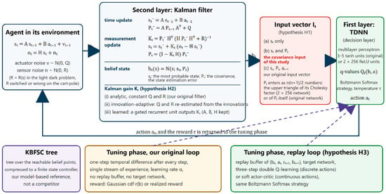
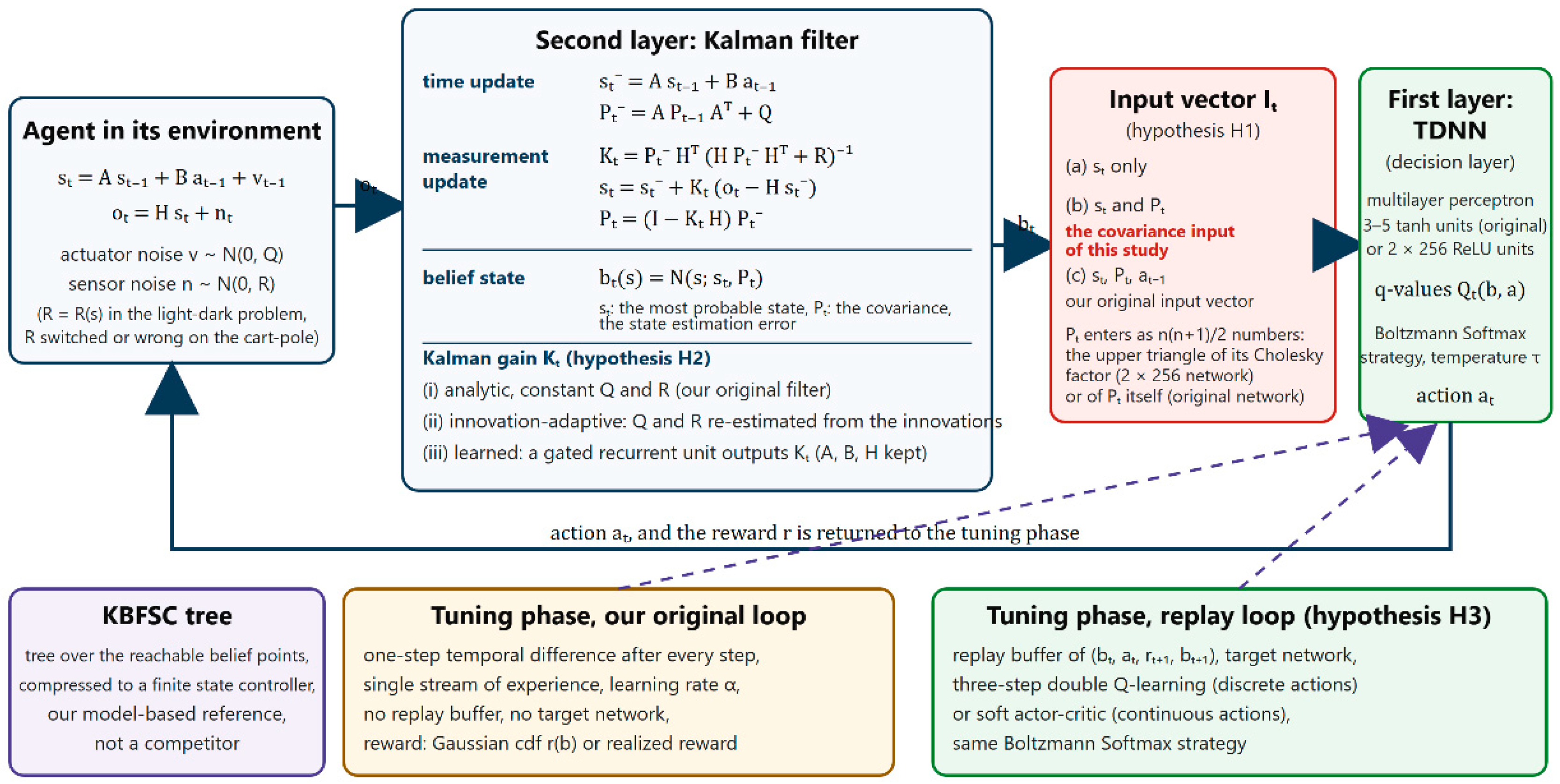
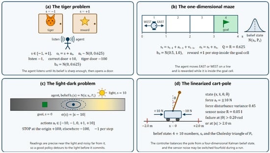
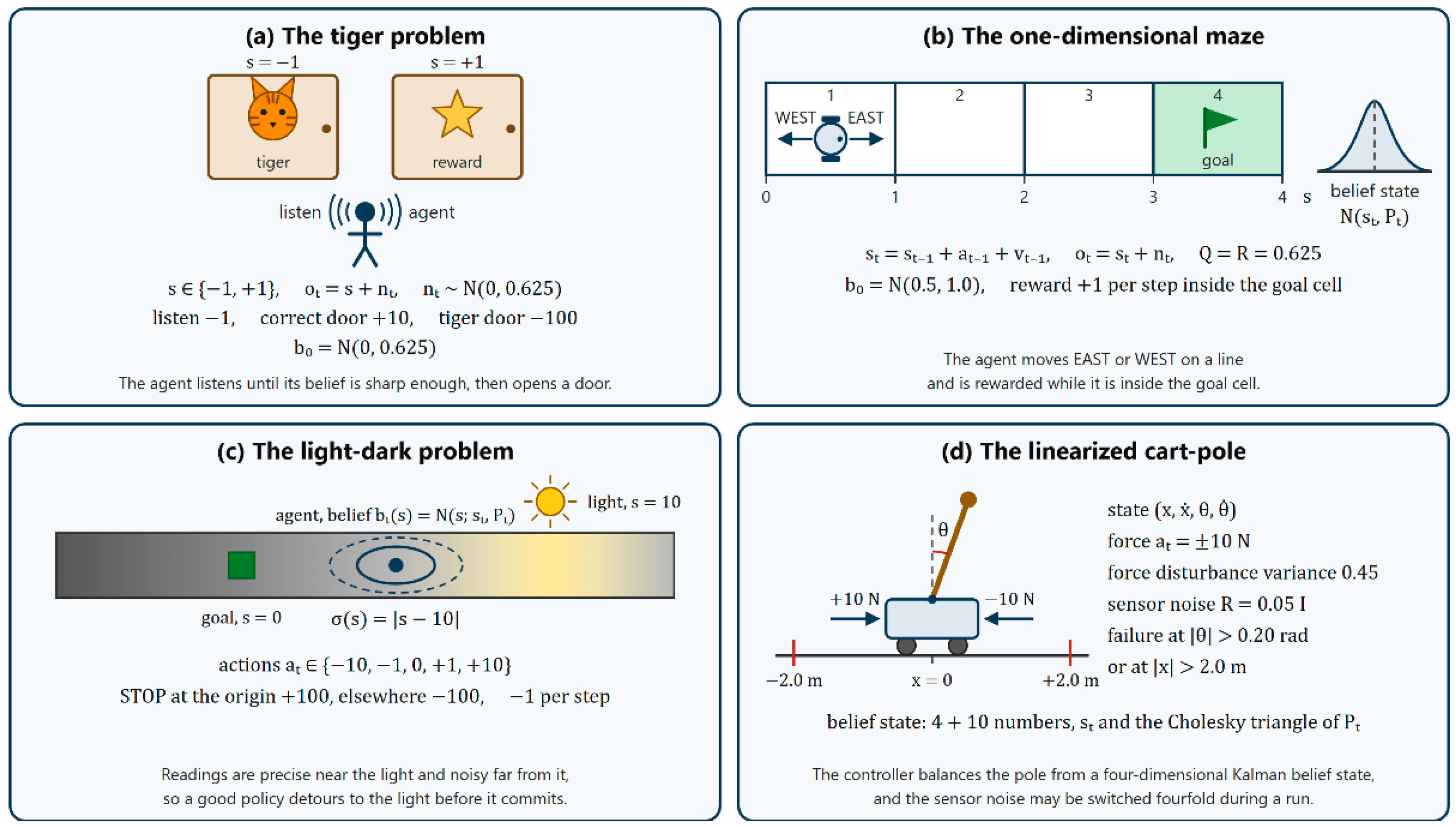
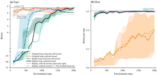
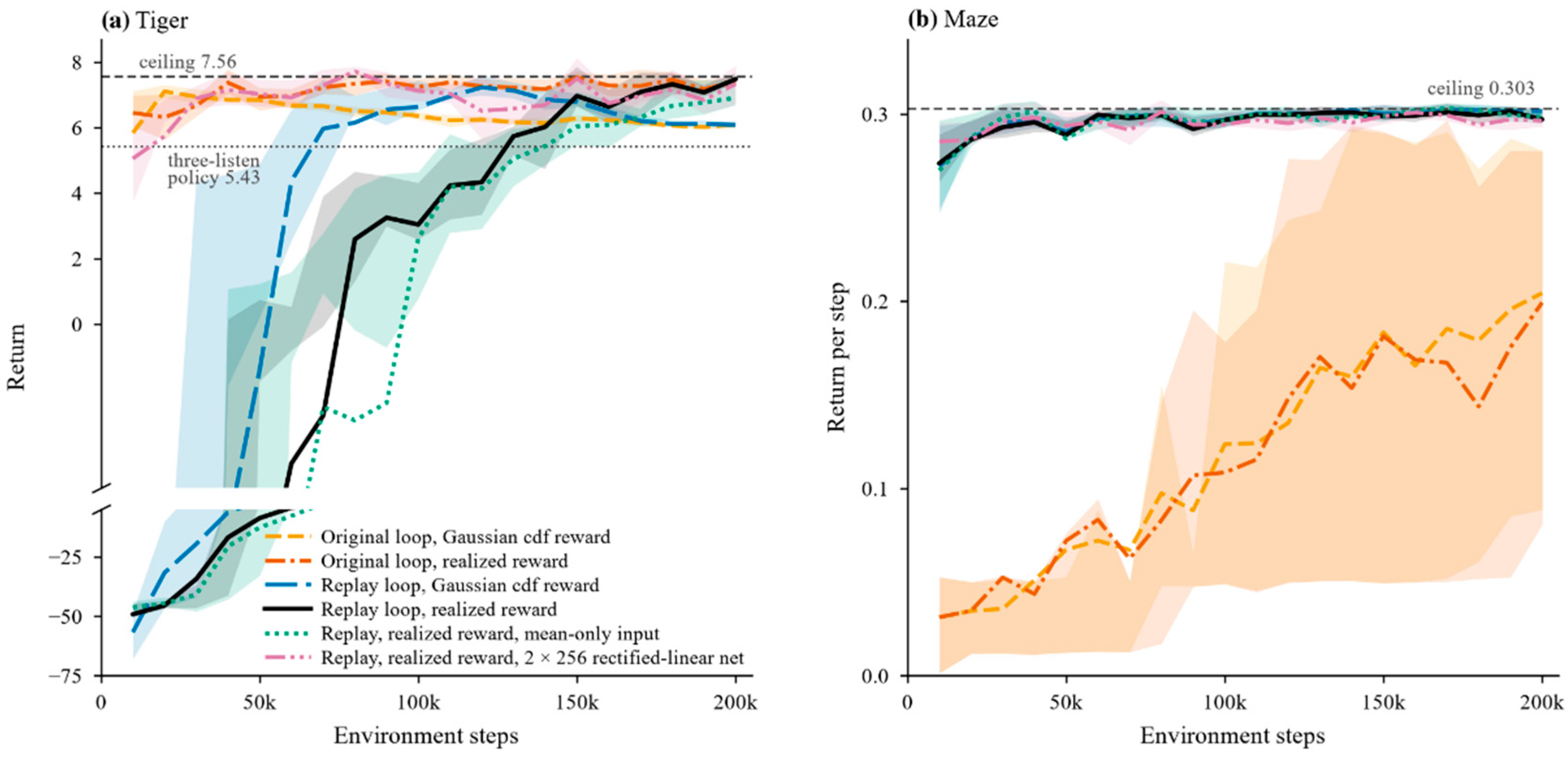
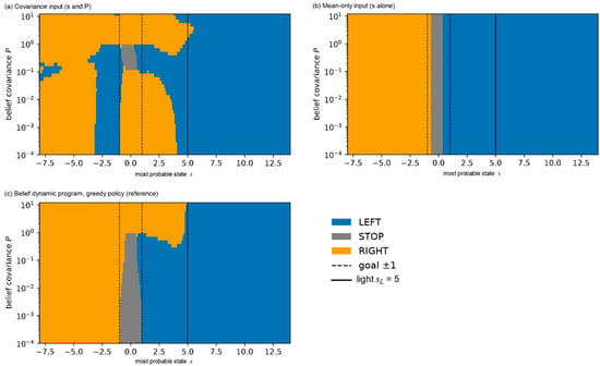
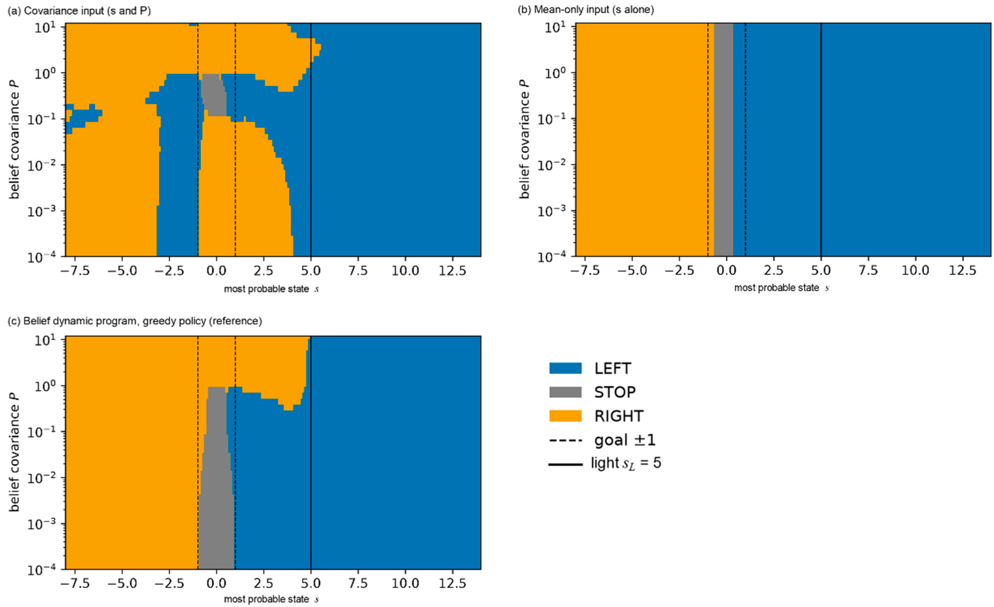
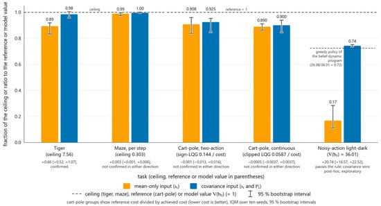
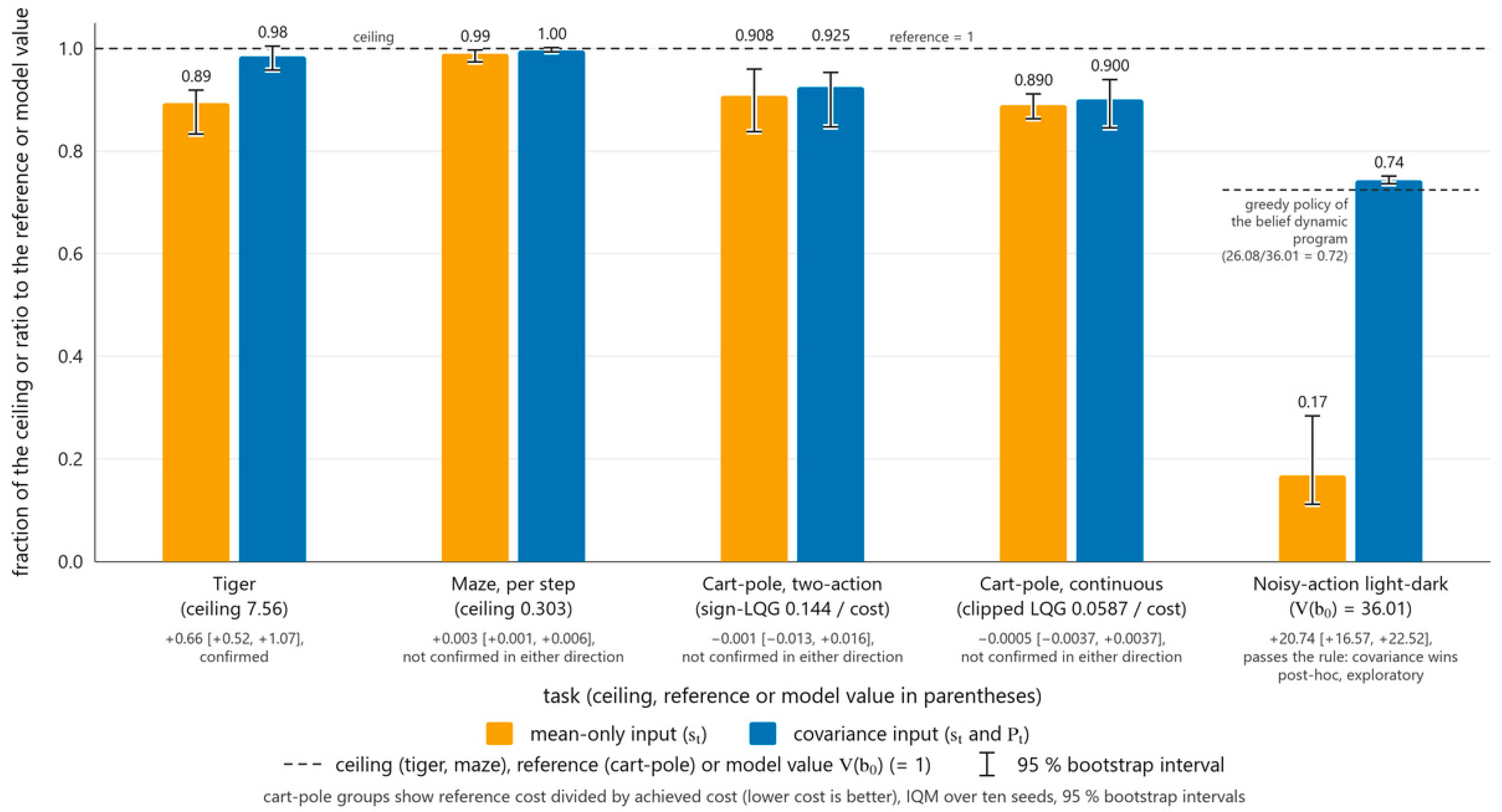

Disclaimer/Publisher’s Note: The statements, opinions and data contained in all publications are solely those of the individual author(s) and contributor(s) and not of MDPI and/or the editor(s). MDPI and/or the editor(s) disclaim responsibility for any injury to people or property resulting from any ideas, methods, instructions or products referred to in the content. |
© 2026 by the authors. Licensee MDPI, Basel, Switzerland. This article is an open access article distributed under the terms and conditions of the Creative Commons Attribution (CC BY) license.