


Abstract
The intersection-of-confidence-intervals edge-preserving lifting (ICI-EPL) transform requires a sensitivity parameter Γ, which is difficult to choose without a clean reference. We select it from a single noisy observation using coupled-bootstrap risk estimation. Each gamma candidate is scored at three noise-inflation levels, with a linear fit providing a zero-inflation score to minimize. This approach leaves adaptive support selection and hard thresholding intact, despite their discontinuities. For independent, identically distributed Gaussian noise with known scale, the positive-inflation score is unbiased for fixed-candidate risk at the inflated variance. Our analysis of the finite ICI-EPL implementation gives a second-order extrapolation bias as the nodes approach zero. Across 120 synthetic signal, length, and noise scenarios comprising 1440 observations, selection reduces mean noise-normalized squared error by 28.13% relative to fixed Γ = 2. Independent risk simulations and repeated selections examine the inflation levels and perturbation count; further tests use misspecified or estimated noise scales and randomly generated signal shapes. Recorded ECG windows with added Gaussian and structured contamination provide an application example.
1. Introduction
The intersection-of-confidence-intervals edge-preserving lifting (ICI-EPL) transform chooses its wavelet predictions locally, using neighborhoods selected from the observed signal [1,2,3]. At each point, the ICI rule compares local polynomial estimates over increasing neighborhoods. A support can grow while the associated confidence intervals retain a common intersection. These support choices guide the lifting predictions in smooth regions and near abrupt changes; denoising then thresholds the detail coefficients and reconstructs the signal using the stored support maps.
The difficulty is choosing Γ, the sensitivity parameter that sets the interval widths. A change in gamma can alter the accepted supports, the lifting coefficients, and which coefficients survive thresholding [3]. Satisfactory local predictions do not by themselves establish that a gamma value gives a good final reconstruction. Yet reconstruction error is unavailable in practice: only the noisy signal is observed.
Several related choices have been addressed in the ICI literature, including weighted-residual cross-validation for local polynomial approximation and modified support-selection rules [1,4,5]. ICI has also been used for local-regression smoothing [6] and to adapt thresholds in sparse wavelet image reconstruction [7]. Those applications concern local smoothing or reconstruction thresholds. In ICI-EPL, gamma governs the transform itself; published studies have chosen it with access to a reference signal [3].
Risk-based tuning offers a way to make such choices without a clean reference. In one-dimensional filtering, for example, John et al. select Savitzky–Golay order or window length using an unbiased mean squared error (MSE) criterion [8]. Stein’s unbiased risk estimation (SURE), together with its wavelet and Monte Carlo extensions, provides reconstruction-risk criteria under suitable regularity conditions [9,10,11]. Regularity is the obstacle here. Even recent scalable SURE evaluation for convex-regularized estimators retains weak-differentiability requirements [12], whereas a small change to an ICI-EPL input can switch a support or move a coefficient across a hard threshold. This makes direct use of derivative-based risk formulas problematic.
Coupled bootstrap (CB) takes a different route: it adds specially coupled Gaussian perturbations to the observation to estimate risk, without requiring a continuous estimator [13]. Oliveira et al. already use it for denoising parameter selection. We use it to score ICI-EPL gamma candidates, but the increased noise variance needs attention. Rather than select gamma at a single inflated variance, we fit a line to scores at three inflation levels and minimize its zero-inflation intercept. This step is analogous to simulation–extrapolation [14], with reconstruction risk as the quantity being extrapolated.
Our contribution is this zero-inflation selection rule. The analysis derives its leading bias for the finite ICI-EPL implementation; the experiments test the gamma choices on synthetic signals and recorded electrocardiograms (ECGs).
2. Observation Model and Reference ICI-EPL Denoiser
2.1. Model and Selection Target
We seek to recover a fixed signal from one noisy observation, under the model
where are the observed and underlying signals, respectively, and n is the number of samples. The noise vector ϵ has independent, identically distributed (iid) Gaussian entries with zero mean and known standard deviation ; is the identity matrix.
Write for ICI-EPL denoising of input z at sensitivity Γ > 0: support selection, lifting, detail thresholding, and reconstruction. All other transform and threshold settings are fixed, but the supports are selected afresh from each input. For one candidate, the target is expected reconstruction error per sample,
The expectation averages over observation noise for the same underlying f. The argument zero denotes the original noise variance; Section 3 also considers risk after adding noise. The unknown f prevents direct evaluation of this objective.
The proposed procedure estimates this objective across gamma candidates and returns , where is the selected value and contains its internal perturbations. The risk of this final reconstruction includes both observation noise and selection randomness.
2.2. Gamma and Local Support Selection
A prediction support specifies which neighboring samples enter a local prediction. In a smooth region, a longer support can reduce noise sensitivity. Across an abrupt change, the same extension can mix incompatible values. The ICI rule decides how far to extend the support by comparing local estimates at increasing sizes [1].
We use J = 3, 4, 5, 6, 7 lifting levels for signal lengths n = 256, 512, 1024, 2048, 4096, respectively. At lifting level j = 1, …, J, let z be the current approximation: the observed signal at the first level and the approximation produced by the preceding level thereafter. At sample i = 1, …, n, candidate supports are indexed by k in increasing size. Suppressing the level index, the degree-zero (constant) local polynomial approximation (LPA) weight vector gives the estimate and operational noise width ; weights outside the support are zero. Each estimate is assigned an interval with half-width . A larger support is accepted provided that all intervals from the smallest support to the current one retain a common intersection of positive width:
Here indexes the tested support prefix. The largest accepted prefix determines the selected support, and is the level-specific value of the base sensitivity . The scaling of across lifting levels is inherited from the normalized ICI-EPL implementation, which multiplies the approximation by after each lifting step. The factor tracks this accumulated amplitude scaling while the nominal σ remains fixed.
For fixed local estimates, increasing gamma widens the intervals and allows support extension despite larger differences between the estimates. Reducing gamma makes the test more restrictive. At later adaptive levels, is an operational noise width: the data-dependent approximation no longer has the original iid Gaussian noise distribution.
2.3. Directional Verification and Adaptive Lifting
ICI-EPL first evaluates left-sided, right-sided, and symmetric supports. It checks a proposed symmetric support against directional supports growing from both boundaries, contracting it when verification fails. This check helps catch local changes that the centered estimate alone represents poorly. Near edges, one-sided Haar prediction is available, including inward prediction at the signal boundaries. Longer predictions use Neville filters with support counts two, four, or six.
The LPA estimates choose the support; the selected lifting filter makes the prediction. Its residual becomes the detail vector, and an update step uses the details to form the next approximation. No downsampling is performed: the implementation retains a detail vector at every level.
The implementation follows the ICI-EPL lifting construction [2,3], with normalized coefficients and a phase-averaged inverse. For a fixed support map, prediction, update, and synthesis are linear operations. The map is stored during decomposition and reused during reconstruction, which propagates the reconstructed approximation through the levels in reverse order.
2.4. Thresholding, Reconstruction, and the Role of Gamma
The adaptive transform changes how noise appears in the detail coefficients, so their scale need not equal the observation-noise scale σ. The threshold magnitude follows the universal wavelet threshold [15,16]. In the present implementation, its scale is estimated separately at each level and coefficients are hard-thresholded:
Here is the median absolute deviation (MAD) estimate of coefficient scale, is the resulting threshold, and is the thresholded version of . Coefficients at or below the threshold in magnitude are set to zero, while larger coefficients are retained. Medians are taken over the n coefficients; the standard normal quantile supplies the scale calibration.
The inverse transform combines the retained terminal approximation with the thresholded details, using the stored support maps. Importantly, is recomputed for every gamma candidate and every perturbed input. It is not the nominal scale σ used for support selection and CB randomization.
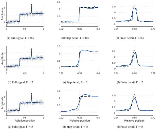
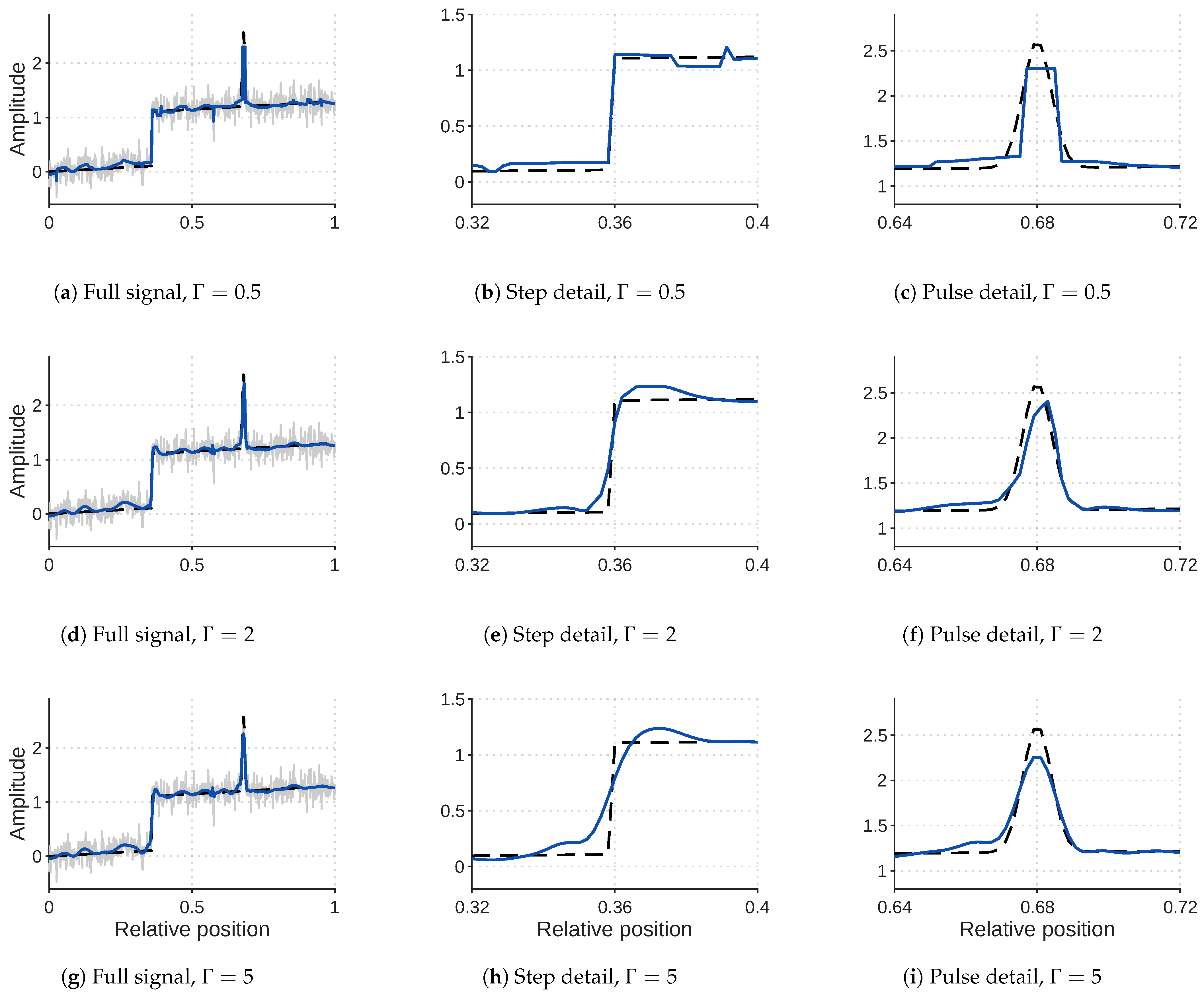
Figure 1 illustrates the effect of gamma at a step and a narrow pulse. Both the residual noise and the shape of the reconstructed features change, although the input and thresholding rule are the same.
Figure 1.
Effect of Γ on a deterministic step-plus-pulse example with 512 samples and σ = 0.16. Panels (a–c), (d–f), and (g–i) use fixed values Γ = 0.5, 2, and 5, respectively, on the same observation. Columns show the full signal, step detail, and pulse detail, with identical axes across rows within each column. Dashed black curves are the reference and blue curves the reconstruction; gray traces show the noisy observation in the full-signal panels.
3. Coupled-Bootstrap Gamma Selection
3.1. Fixed-Candidate Risk at Positive Inflation
An independent second observation of f would give us a way to score a reconstruction: measure their squared discrepancy, then subtract the scoring noise variance. We do not have that observation. CB constructs a pair with the required independence from the available observation and an added perturbation.
For a dimensionless noise-inflation parameter , draw B independent perturbation vectors , , independently of Y, and form
Both vectors have mean f, with coordinate variances and , respectively. Since , joint Gaussianity gives independence under the joint law of Y and , though not conditional on Y.
The per-sample CB score [13] is
The subtractions remove the scoring-noise contribution in expectation. For a fixed candidate whose reconstruction has finite second moments, independence gives
Here denotes risk per sample at observation variance . The left expectation is over Y and the perturbations, and the right expectation is over from Equation (1).
Only the input distribution is inflated. The nominal scale supplied to remains at every level, with supports and coefficient-scale estimates still recomputed from the input.
For numerical evaluation, expand the squared norm in Equation (6). With residual at fixed a and , the contribution of perturbation b becomes
Then . This avoids subtracting large squared norms at small a.
3.2. Extrapolation and Its Approximation Error
Taking a very small brings the target variance closer to the original one but makes noisier. We use three nonzero levels, a ∈ {0.05, 0.1, 0.2}, and extrapolate: an ordinary-least-squares line through the three scores gives an intercept that estimates original-noise risk. On the gamma grid , the fitted intercept and selected gamma are
These are the ordinary-least-squares intercept weights for the three nodes. We use the same B perturbations for every gamma and inflation level. In the following, CB refers to the selector with this extrapolation step.
The remaining question is whether risk is smooth enough to justify this extrapolation when the denoiser itself is discontinuous. For the implementation considered here, input length, decomposition depth, filter bank, nominal scale, and threshold rule are fixed. There are then only finitely many possible support maps and threshold masks.
For a fixed gamma and support map s, let be the analysis matrix that stacks the terminal approximation and all details, and let be the synthesis matrix using that map. Hard thresholding inserts a diagonal zero–one mask H, with ones on the terminal approximation. In exact arithmetic, the resulting reconstruction can therefore be written as
The norm is the induced Euclidean operator norm. The maximum is over finitely many support maps and masks, so there is a constant C, independent of z, with . The selection decisions are measurable, and the squared loss grows at most quadratically.
Now write as an integral of the loss against the Gaussian input density. This integral extends to a > −1. On compact subintervals, the density and its first two variance derivatives have integrable polynomial-times-Gaussian bounds, so differentiation can pass under the integral. It acts on the density, not on the denoiser. The risk is therefore twice continuously differentiable near zero, as required by the smoothness conditions in [13].
For a base inflation , let denote the intercept for nodes and weights . Writing the relative node positions as and the weights as , where component index gives , , , and . By Equation (7), the expected fitted intercept is the same weighted combination of the risks . Taylor expansion at zero therefore cancels the linear inflation term and gives, as ,
where primes denote derivatives with respect to inflation a, and the remainder divided by tends to zero as . The implemented nodes correspond to . If a finite curvature bound M satisfies for , bounding each Taylor remainder and summing with the absolute weights gives an absolute bias of at most .
3.3. Implementation and Simulation Error
For each shared perturbation, we run ICI-EPL on at every gamma and inflation level, keeping the nominal scale and the transform and threshold rules fixed. Each call repeats support selection and verification, lifting, coefficient-scale estimation, thresholding, and reconstruction. Averaging Equation (8) over the B draws gives the score for each gamma–inflation combination.
We combine the three scores using Equation (9) and choose the gamma with the smallest intercept. Exact ties go to the smallest grid value. The final denoising call uses the original observation Y, not a perturbed input, and returns the reconstruction together with score diagnostics. The primary setting uses perturbations and the 46-candidate gamma grid in Equation (9).
Simulation error must respect this pairing. The independent replicates are the B perturbations, not the individual gamma–inflation scores: all scores from one perturbation belong together. For nodes and weights , define one perturbation’s contribution and the estimated conditional Monte Carlo standard error of by
where denotes an estimated standard error conditional on the observed Y, and is the sample standard deviation over the B draws, requiring . For two fixed candidates , the estimated standard error of their intercept difference is .
More perturbations reduce the conditional simulation variance of the score at rate ; they do not remove observation-noise variability or extrapolation bias [13]. Nor should the minimum fitted score be read as an unbiased assessment of the selected reconstruction, because it is subject to selection optimism [17]. We assess reconstruction performance on independent test observations.
4. Experimental Design
The main comparison asks whether choosing gamma for each observation improves on a fixed setting. Separate experiments examine risk estimation, simulation settings, and departures from the primary signal and noise conditions (Table 1).
Table 1.
Experimental design and primary settings.
4.1. Primary Experiment
We use six signals from WaveLab-compatible generators: Blocks, Bumps, Doppler, HeaviSine, Piece-Polynomial, and Piece-Regular [18]. The lengths are n ∈ {256, 512, 1024, 2048, 4096}, and noise standard deviations are {0.05, 0.10, 0.15, 0.20} times the clean-signal range (maximum minus minimum amplitude). These choices give 120 fixed scenarios. Twelve fresh Gaussian observations in each scenario produce 1440 independent inputs.
Throughout the experiments, “noise/range” means noise standard deviation divided by the clean-signal range, and grid notation follows start:step:end. We use Gaussian draws as generated, without rescaling their realized norms. CB and the controls are compared on the same observations, with the same supplied scale, transform, and threshold policy, so the comparisons are paired [19].
Before confirmation, we fixed the configuration and sample design: universal hard thresholding, with the gamma grid, inflation nodes, and budget given above. The main fixed control is Γ = 2. Because the apparent gain could depend on this choice, we also report descriptive results at Γ = 0.5, 1.0, …, 5.0 and for the best fixed value on the full spacing- grid, calculated from the saved candidate sweeps on the same confirmation observations. CB selects gamma separately for each observation on the full grid. The clean signal is used only for evaluation, including the grid-oracle loss defined in Section 4.6.
4.2. Risk Validation, Inflation, and Conditional Simulation Studies
To check the scores against risk, we use 12 scenarios spanning the six canonical signals, lengths, and noise levels (Table 2). At the original variance and each inflated variance, 1000 independent draws give a risk-reference curve. We compare it with scores from 100 separate observations per scenario, holding the nominal denoiser scale fixed across variances.
Table 2.
All 12 risk-validation settings and the gamma values minimizing the estimated mean extrapolated score and original-variance risk on the grid Γ = 0.5:0.1:5. Mean scores use 100 independent observations with eight perturbations per inflation level; risk references use 1000 independent draws at the original variance. Noise/range is σ divided by the clean-signal range.
For each scenario, bias is estimated at each gamma candidate as the mean score over 100 observations minus the corresponding independent risk reference. Candidate-averaged bias is the arithmetic mean of these 46 signed estimates. The reported range is taken across the 12 scenario averages. We report candidate-averaged bias and reference Monte Carlo standard error in units of ; score variance, which includes both observation and perturbation randomness, is reported in units of .
The inflation experiment uses 30 fresh observations of each of Blocks, Bumps, Doppler, and Piece-Polynomial at n = 256 and noise/range 0.1. We fit linear intercepts on three node grids: (0.01, 0.025, 0.05), (0.025, 0.05, 0.1), and (0.05, 0.1, 0.2), at B ∈ {8, 64, 128}. All nine configurations use the same 120 observations. Within each observation, perturbations are shared across grids and gamma candidates, and the smaller budgets use prefixes of the same 128 draws. We report paired loss differences relative to the primary node grid at each budget, using the stratified intervals in Section 4.6. The primary confirmation experiment uses B = 8.
For the perturbation-count experiment, we keep four noisy inputs fixed and repeat selection with 20 independent seeds at each B ∈ {4, 8, 16, 32, 64, 128}.
4.3. Noise-Scale Sensitivity
We generate 12 Gaussian observations for each of the six canonical signals at n = 512, with σ = 0.1 times the signal range. The nine conditions (Section 5.4) supply a scale through fixed ratios {0.70, 0.85, 1, 1.15, 1.30}; the sample standard deviation of 32, 128, or 512 independent Gaussian calibration samples; or the same-observation estimate
where , , are successive first differences. Differencing removes locally constant signal components, and the denominator accounts for the noise increase under independent Gaussian sampling. Signal changes also contribute to these differences and can bias the scale estimate.
We hold the supplied scale fixed across candidates and inflation levels, using it for both CB perturbations and ICI support selection. The coefficient-MAD threshold scales are still recomputed within each call. The oracle uses the same supplied scale and candidate family as CB, while loss normalization uses the true generating variance.
4.4. Random Signal Morphologies
The additional signals come from four families: piecewise quadratics with random breaks and coefficients; five Gaussian pulses with variable widths, amplitudes, clustering, and boundary placement; amplitude-modulated chirps with randomized phase and sweep rate; and three damped oscillatory transients on a weak trend.
For each family, we generate 24 clean morphologies, evenly divided among n ∈ {256, 512, 1024}, and two Gaussian observations per morphology at noise/range 0.10. Half of the morphologies use irregular coordinates. ICI-EPL nevertheless operates on sample indices, so these cases deliberately introduce coordinate mismatch. We average the two losses for each clean morphology and weight the four families equally.
4.5. ECG Application
The ECG experiment measures reconstruction after adding contamination to recorded windows; the recordings before this addition serve as references. We use the MIT-BIH Arrhythmia and Noise Stress Test databases [20,21,22,23], obtained through PhysioNet [24]. After excluding eight development records, the evaluation uses 35 held-out records, each with four nonoverlapping 2048-sample windows at 360 Hz. Added white Gaussian noise (AWGN) has standard deviation 0.05 or 0.10 times the recorded reference range. Baseline wander, muscle artifact, and electrode-motion traces each have root mean square (RMS) 0.10 times that range. We keep the CB settings and ICI-EPL configuration unchanged across windows.
The preferred lead is modified limb lead II (MLII), with one-based window starts at samples 3601, 36,001, 108,001, and 216,001 . Window eligibility requires at least three annotated beats, a peak-to-peak reference amplitude strictly between 0.2 and 8 mV, and the first-difference scale from Equation (12) divided by that range no greater than 0.04. Development records 100, 101, 103, 105, 106, 108, 109, and 111 are excluded, along with paced records 102, 104, 107, and 217. Record 202 is excluded because it shares a subject with record 201. All 35 eligible held-out records are included; the archive records their identifiers.
These references retain their native acquisition noise. CB sees only the contaminated window and the supplied added-noise scale, not the beat annotations, which are used for window eligibility. We average window-level ratios within each record and calculate intervals from the 35 record means.
4.6. Loss and Uncertainty
For a reconstruction of f, noise-normalized mean squared error (NMSE) is
Mean NMSE averages this loss over the experimental units described above.
Control comparisons pair losses from the same observation. Let be the CB-minus-control loss difference for observation r in scenario s, with within-scenario sample mean , sample variance , and observation count . For S equally weighted fixed scenarios,
Here is the mean loss difference and its estimated standard error. Pointwise 95% normal-approximation intervals use . Intervals for mean NMSE use the same calculation with individual losses in place of paired differences. Morphology and ECG intervals instead use independent morphology and record units, respectively.
The grid oracle selects the gamma with the smallest squared error against the clean signal for each observation Y. The ratio of CB loss to oracle loss is
We average these per-observation ratios to obtain the mean oracle ratio. This oracle minimizes realized error separately for each observation; it is not the fixed-candidate expected risk .
5. Results
5.1. Primary Gamma-Selection Performance
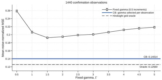
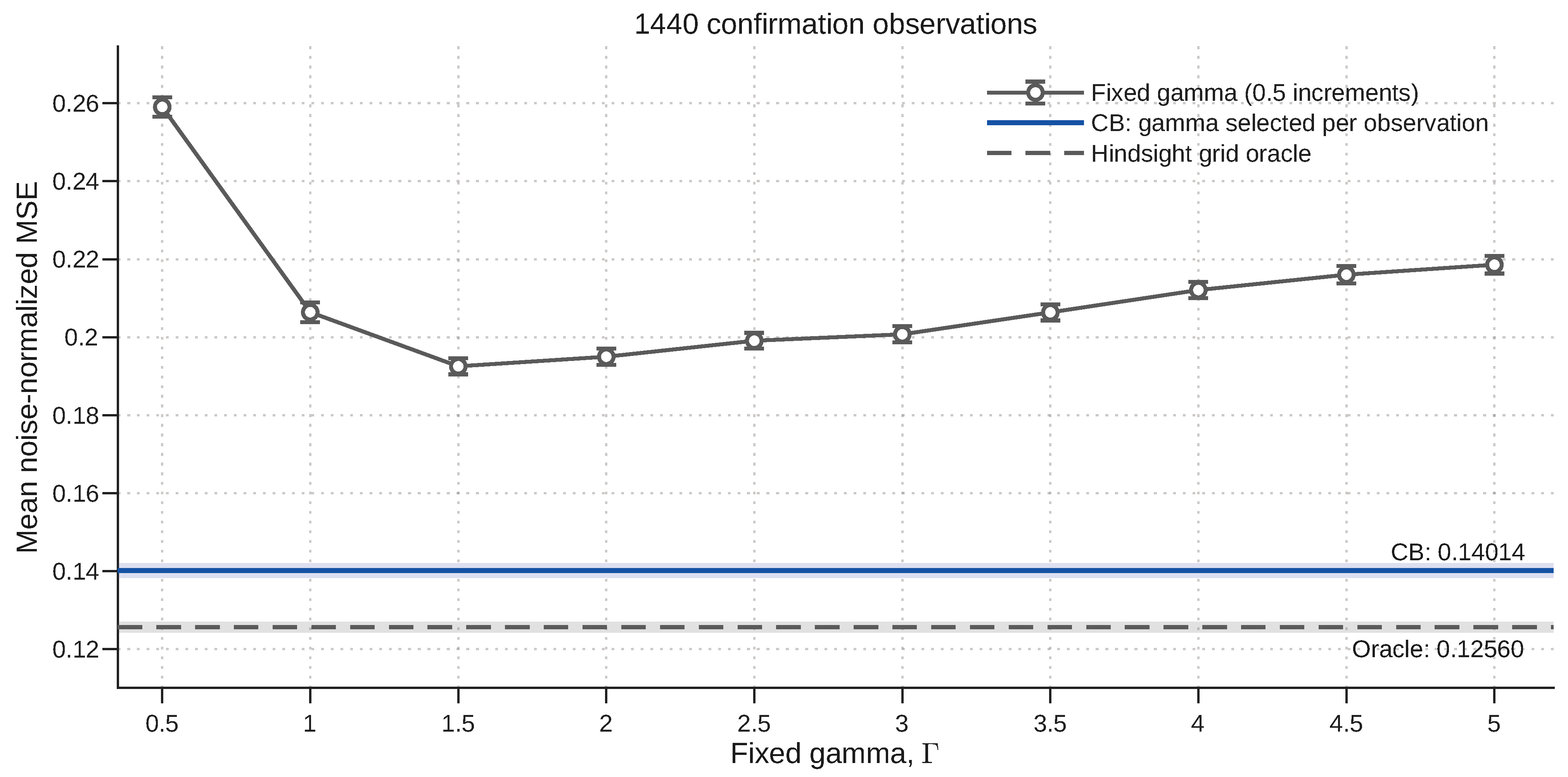
CB achieves mean noise-normalized MSE 0.14014, compared with 0.19498 for fixed : a reduction of 28.13%. The paired mean difference is −0.05484, with 95% interval [−0.05688,−0.05280]. The grid-oracle mean loss is 0.12560.
For descriptive comparison, the lowest mean NMSE among the fixed settings displayed in Figure 2 is 0.19252 at Γ = 1.5. On the full spacing-0.1 grid, it is 0.19164 at Γ = 1.7, compared with 0.14014 for CB.
Figure 2.
Fixed-gamma reconstruction loss on the same 1440 confirmation observations from 120 fixed scenarios. Circles show Γ = 0.5, 1.0, …, 5.0. Each fixed value is used for every observation. Error bars are pointwise stratified 95% normal intervals for mean NMSE. Horizontal lines and shaded pointwise intervals show CB and the hindsight grid oracle, both of which choose gamma separately for each observation on the original 0.5:0.1:5 grid; only the oracle uses the reference signal. Connecting segments guide the eye between displayed fixed settings.
5.2. Oracle Proximity and Selection Tails
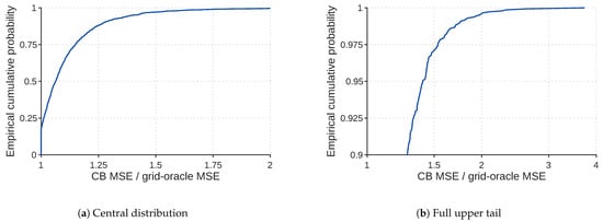
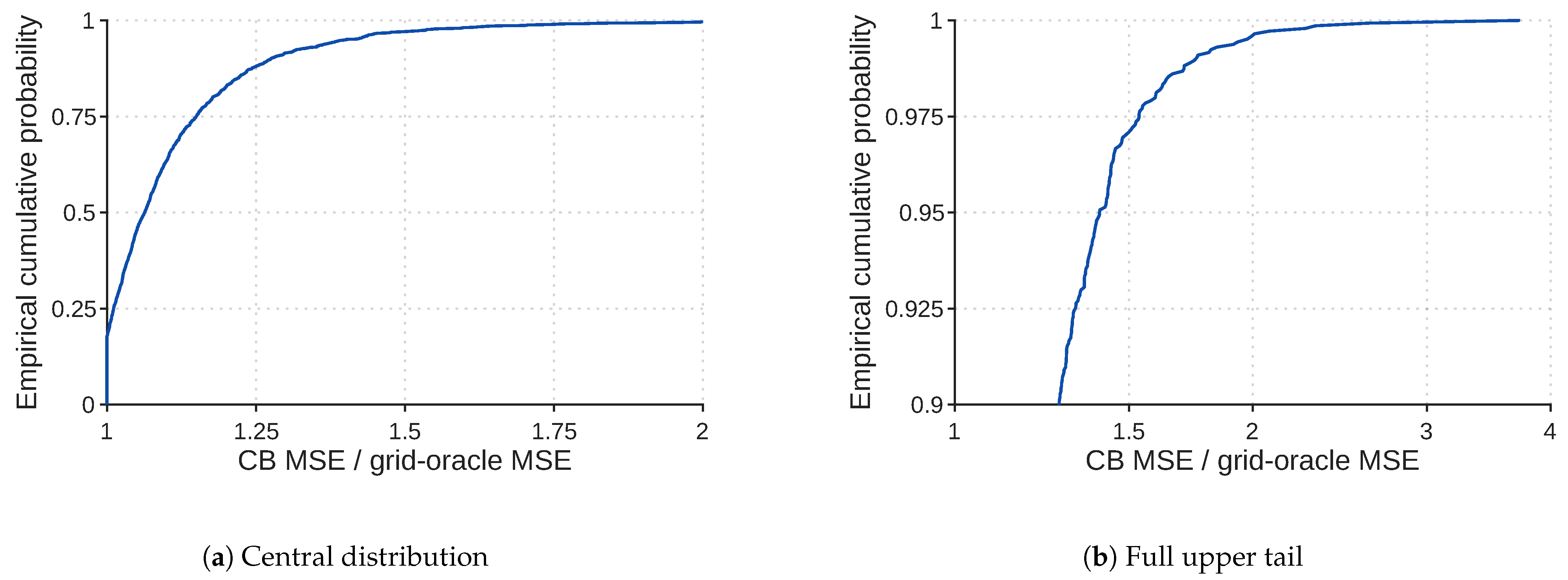
The median CB-to-oracle loss ratio is 1.0633, and 63.4% of observations fall within 10% of oracle loss. The upper tail pulls the mean ratio to 1.1132. At the 90th percentile the ratio is 1.2750; six of the 1440 observations exceed twice the oracle loss. The largest observed ratio is 3.7251 (Figure 3).
Figure 3.
Distribution of CB loss divided by the ICI-EPL grid-oracle loss for each of the 1440 confirmation observations. (a) Central distribution. (b) Upper tail with a logarithmic horizontal axis, retaining the full observed range.
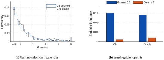
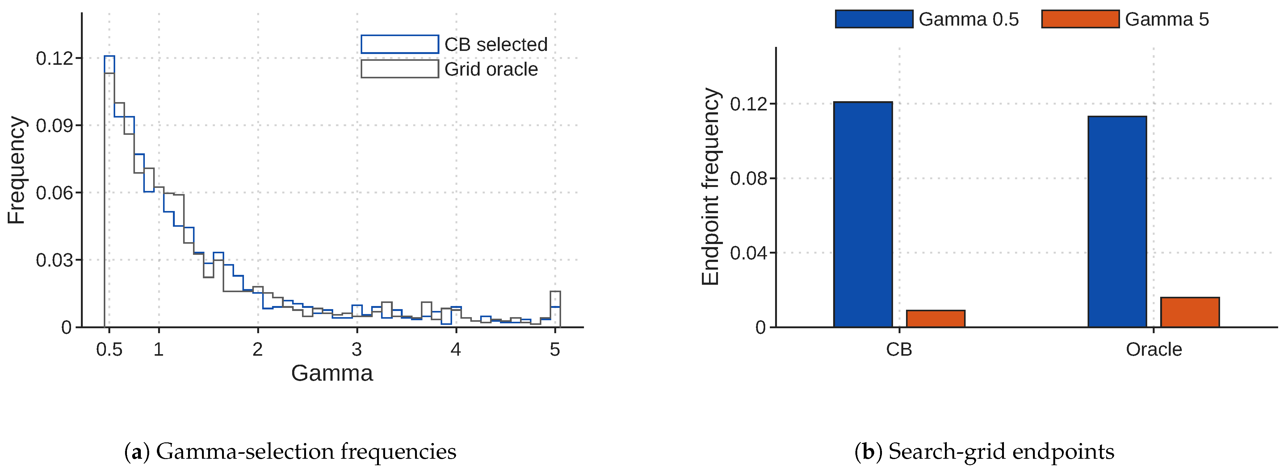
Small gamma values are common in both distributions in Figure 4: about 71% of CB and oracle choices are at or below Γ = 1.5, although the rest extend over much of the grid. The lower-end peak is not confined to CB. It selects that endpoint on 12.1% of observations, against 11.3% for the oracle. Either method selects the upper endpoint on fewer than 2% of observations.
Figure 4.
Gamma selection on the 46-value confirmation grid. (a) Selection frequencies. (b) Proportions selecting the lower and upper endpoints. CB and the hindsight grid oracle use the same 1440 inputs and candidate reconstructions.
5.3. Risk Validation and the Inflation–Simulation Tradeoff
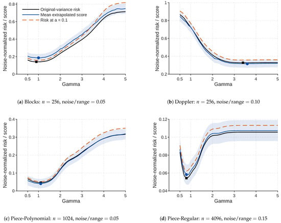
Figure 5 compares the mean extrapolated score with independent risk estimates at the original variance and at inflation a = 0.1. The Blocks score is visibly above the original-risk curve across much of the grid. Its minimum is nevertheless nearby: Γ = 1.0 for the mean score, against Γ = 0.9 for risk. The corresponding Doppler minima are 3.6 and 3.4. They coincide for Piece-Polynomial at 1.1 and for Piece-Regular at 0.8. Table 2 gives both minimizers for all 12 scenarios.
Figure 5.
Four scenarios from the 12-scenario risk-validation study; noise/range denotes σ divided by the clean-signal range. Black curves show independent original-variance risk, blue curves mean extrapolated scores, and dashed orange curves independent risk at inflation a = 0.1. Risk and score ordinates are divided by . Reference curves use 1000 draws; mean scores use 100 independent observations with eight perturbations per inflation. Shading gives pointwise 95% normal Monte Carlo intervals. Black squares and blue circles identify minima of the original-risk and mean-score curves, respectively.
Doppler also has a broad low-risk region, unlike the more distinct small-gamma minimum of Piece-Regular. The same displacement in gamma can therefore have quite different consequences for reconstruction error.
Across the 12 diagnostic scenarios, the mean estimated CB bias over the 46 gamma candidates ranges from −0.01417 to 0.04565 in noise-normalized units. Candidate-averaged score variance ranges approximately from 0.00316 to 0.06103, while mean reference Monte Carlo standard errors range from 0.000068 to 0.002744.
Moving the inflation nodes closer to zero did not help at eight perturbations (Table 3). On the four-family, n = 256 design, mean normalized MSE rises from 0.31767 for the primary grid to 0.33378 for (0.025, 0.05, 0.1) and 0.37993 for (0.01, 0.025, 0.05). Both paired intervals at B = 8 are above zero, with the larger increase occurring for the smallest grid.
Table 3.
Inflation-grid sensitivity at three perturbation budgets on the same 120 inputs. Each fit uses three nodes and B common draws per node. Differences and pointwise 95% paired intervals are relative to the primary grid at the same B.
At B = 64 and 128, the primary-grid mean losses decrease to 0.30206 and 0.30018, respectively. The middle-grid loss differences are 0.00111 and 0.00200, with paired intervals that include zero. The smallest-grid differences are 0.00925 and 0.00444; both pointwise intervals are above zero, although the lower bound at B = 128 is only 0.00006. Thus, the observed penalties for smaller nodes are reduced at larger budgets, while the primary grid retains the lowest pooled mean loss at each tested budget. The middle-grid intervals do not establish equivalence.
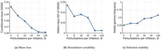
To examine simulation variability conditional on the observed data, Figure 6 repeats selection on four fixed observations. Mean CB loss decreases from 0.28788 at eight draws to 0.26181 at B = 64 and 0.26113 at B = 128, with inflation nodes unchanged. The spread over repeated selections does not fall at every step. Mean within-input standard deviation first rises from B = 8 to B = 16, then decreases at the larger budgets.
Figure 6.
Conditional simulation stability for four fixed observations with 20 independent selector seeds at each budget. (a) Mean noise-normalized loss. (b) Within-input standard deviation (SD) of loss. (c) Modal gamma frequency: the fraction of the 20 selections equal to the most frequent gamma for each input. All panels average their summaries over the four inputs. Only the number of common perturbations B per inflation level changes; the CB score, inflation grid, and gamma grid remain fixed.
Mean within-input standard deviation is about 0.0049 at both B = 64 and B = 128. Over that same increase in budget, average modal gamma frequency rises from 48.75% to 57.5%: agreement on gamma continues to improve after mean reconstruction loss has nearly leveled off.
5.4. Noise-Scale Sensitivity and New Morphologies
Using the correct scale gives CB mean normalized MSE 0.20372 and mean oracle ratio 1.1359 (Table 4). The same-observation plug-in estimate is close on these signals, with loss 0.20513 and mean ratio 1.1436. Independent calibration samples also give losses near the known-scale value, though not an orderly improvement with larger calibration samples.
Table 4.
CB sensitivity to the supplied noise scale under iid Gaussian observation noise. Each condition includes six signals and 12 independent observations per signal. Intervals are pointwise.
Deliberately supplying 70% of the true scale raises the mean oracle ratio to 1.2640; supplying 130% gives 1.1745. The absolute losses at these two 30% errors are almost the same—0.21456 and 0.21484. Their oracle ratios use different candidate reconstructions, each obtained with the scale supplied in that condition.
Across 96 independent clean morphologies, mean loss is 0.85747 for CB (95% interval 0.73516–0.97978) and 0.82486 for the ICI-EPL grid oracle (0.70325–0.94648). The mean per-observation oracle ratio is 1.1274.
Chirps account for much of the pooled absolute error. Their mean CB and oracle losses are 2.84568 and 2.79476, while the mean per-observation oracle ratio is 1.0274, the smallest among the four families. The ratio of the mean losses is 1.0182. Pulses are reconstructed with much lower CB loss, 0.17693, yet have the largest mean oracle ratio, 1.2243.
5.5. Gamma Selection on Recorded ECG
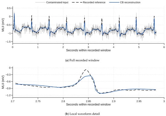
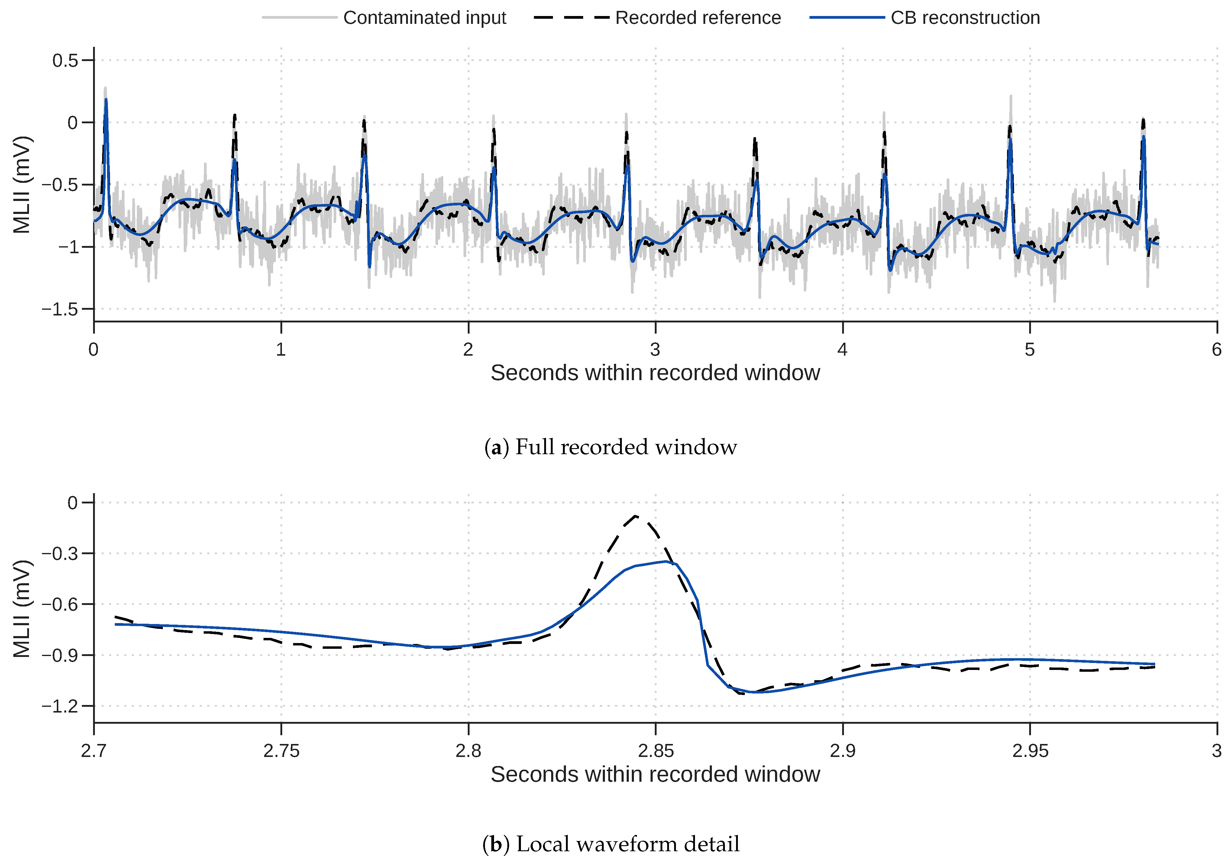
For added-Gaussian noise/range 0.05 and 0.10, the recorded ECG windows give mean CB-to-oracle loss ratios of 1.0396 and 1.0694, respectively (Table 5). Window-level ratios are averaged within records and then across records; for AWGN 0.10, the ratio of the mean losses is 1.0507. In the record-112 example (Figure 7), both methods choose Γ = 1.7. Much of the added fluctuation is removed. The enlarged detail shows a rounded positive peak.
Table 5.
Gamma selection on 35 held-out ECG records: CB reconstruction loss and comparison with the ICI-EPL grid oracle.
Figure 7.
CB gamma selection on a window from record 112 with added Gaussian noise of standard deviation 0.10 times the recorded reference range. (a) Full window. (b) Local detail. The reconstruction uses ; the hindsight grid oracle chooses the same gamma for this observation.
For baseline wander, leaving the contaminated input unchanged would give lower mean error than either reconstruction. The CB and oracle normalized losses are 1.0777 and 1.0646, both above one, although the mean oracle ratio is only 1.0121.
Muscle-artifact losses remain close to the unchanged-input value: 0.98877 for CB and 0.97462 for the oracle. Electrode-motion losses are lower, at 0.91331 and 0.87790. None of these artifact conditions reaches the much lower noise-normalized losses of the added-Gaussian cases.
6. Discussion
The gain in the primary experiment is not just a consequence of using Γ = 2 as the control. CB also has lower mean loss than the fixed settings in the most favorable part of the profile. What changes is the choice of gamma, not the lifting or thresholding rule. This matters because the oracle choices vary substantially across observations (Figure 4); one fixed value cannot be optimal for all the tested shapes and noise levels. CB makes this choice from the observation and supplied noise scale, without needing the clean reference.
The criterion also leaves the existing ICI-EPL implementation intact. We do not replace support verification or hard thresholding with smooth approximations to make the risk calculation work. Their effects enter through the reconstructed signal that CB scores.
The smoothness needed for extrapolation is a property of the averaged risk, not of an individual reconstruction. The finite-filter argument makes that distinction precise: at fixed gamma, Gaussian averaging yields a smooth function of observation variance even when reconstructions jump. The linear fit cancels the first-order inflation term, leaving a second-order bias as the nodes approach zero. This is a statement about expected scores for fixed candidates, not a claim that the minimum fitted score is unbiased for the reconstruction selected from it.
Bias affects candidate ranking through its variation across candidates, since a shared offset cancels. For the Blocks example in Figure 5, the estimated noise-normalized offsets at Γ = 0.9 and 1.0 are similar (0.04626 and 0.04576). The positive offset does not imply that bias increases with Γ; the estimated bias is nonmonotonic across the grid. The bias expansion links candidate-dependent bias to risk curvature with respect to inflation. With Doppler’s broad minimum, a different gamma can produce almost the same error. The budget experiment shows a related effect, with gamma frequencies still changing after mean loss has nearly stabilized.
That does not make all selection disagreements harmless. The upper tail in Figure 3 contains observations with a substantial loss penalty, which a mean alone obscures. Gamma stability and reconstruction accuracy answer different questions and need to be read separately.
The joint comparison in Table 3 shows reduced loss penalties for smaller nodes at larger budgets, although the primary grid retains the lowest pooled mean loss at each tested budget. For nodes t(1, 2, 4), the leading extrapolation bias is proportional to , but smaller nodes can amplify Monte Carlo variability through the score term. Increasing B reduces conditional simulation variance at rate while leaving extrapolation bias unchanged. For three inflation levels, scoring requires denoiser evaluations, where is the number of gamma candidates. These results characterize three grids at three budgets and do not establish a globally optimal combination. The apparent plateau in mean reconstruction loss near B = 64 in Figure 6 applies only to its fixed nodes and four observations.
For a close choice between candidates, Equation (11) gives a useful diagnostic: the Monte Carlo standard error of their score difference, with the pairing retained. Looking at either score’s variability in isolation misses that pairing. Antithetic randomization has been studied as a way to control small-inflation variance under weak differentiability and moment assumptions [25]. The present experiments use independent perturbations; an antithetic version of the selector was not tested.
An incorrect noise scale changes more than the risk score. It also changes the ICI interval widths and hence can change the candidate reconstructions. The oracle comparison then has a different baseline, explaining why the two 30% scale errors give similar absolute losses but different relative gaps.
The exact CB identity still requires the true scale for covariance cancellation. We tested a first-difference plug-in estimate. It performed close to the known-scale setting on these signals, suggesting that a separate calibration recording may be unnecessary in such cases. Frequent signal changes can enter that estimate, however, so this empirical agreement does not extend the known-scale identity to the plug-in procedure.
The pulse and chirp results point to different limits. For pulses, the larger relative gap leaves room for better gamma selection within the present candidate family. For chirps, even the oracle reconstructs poorly. A more accurate selector cannot remove error that is already present in its best available candidate; substantial improvement there requires changing the denoiser family.
The Gaussian-contaminated ECG windows extend the selection results to recorded waveform shapes while retaining the added-noise model used in the derivation. The structured artifacts are a different test, outside that model. Their small oracle gaps should not be mistaken for effective artifact removal: even the oracle is worse than the unchanged input for baseline wander and improves little on muscle artifact.
There is also a waveform-level limitation. CB and the oracle agree on gamma in Figure 7, but the positive peak is rounded. Agreement with the MSE oracle is therefore not enough to establish preservation of local ECG morphology. Clinical noise evaluation also uses diagnostic criteria [26], which are not measured by the reconstruction losses reported here. More generally, low MSE does not guarantee preservation of important features in other signal classes; morphological fidelity requires separate evaluation using criteria appropriate to each signal class and its intended application.
7. Conclusions
We select ICI-EPL gamma from a single noisy observation by minimizing a linearly extrapolated coupled-bootstrap score. In the canonical-signal experiment, this gave lower mean reconstruction loss than every displayed fixed-gamma setting, with many selections close to the grid oracle. The selected gamma is then used to denoise the original observation.
The theoretical guarantee has a specific scope: iid Gaussian noise with known scale, and risk for a fixed candidate. At positive inflation, the score is unbiased for risk at that variance. The finite-filter argument justifies linear extrapolation despite the denoiser’s discontinuities and gives a second-order residual bias as the nodes approach zero.
In practice, the inflation nodes cannot be chosen independently of the simulation budget. Smaller nodes increased reconstruction error at eight perturbations, while additional draws improved repeated-selection performance on the four fixed inputs. The estimated-scale and recorded-ECG tests broaden the empirical evaluation, but gamma tuning has a clear limit: it cannot repair a candidate family that already reconstructs poorly at its oracle setting. The tested chirps and baseline wander expose that limit.
Author Contributions
Conceptualization, M.T.; methodology, M.T.; software, M.T.; formal analysis, M.T. and M.G.; investigation, M.T.; writing—original draft preparation, M.T.; writing—review and editing, M.T. and M.G.; funding acquisition, J.L. All authors have read and agreed to the published version of the manuscript.
Funding
This research received no external funding.
Institutional Review Board Statement
Not applicable.
Informed Consent Statement
Not applicable.
Data Availability Statement
The dataset used in the analysis is available at https://doi.org/10.5281/zenodo.23259171 (accessed on 9 October 2026).
Conflicts of Interest
The authors declare no conflicts of interest.
References
- Katkovnik, V. A New Method for Varying Adaptive Bandwidth Selection. IEEE Trans. Signal Process. 1999, 47, 2567–2571. [Google Scholar] [CrossRef] [Scilit]
- Tomić, M.; Seršić, D. Adaptive edge-preserving denoising by point-wise wavelet basis selection. IET Signal Process. 2012, 6, 1–7. [Google Scholar] [CrossRef] [Scilit]
- Tomić, M.; Seršić, D. Point-Wise Adaptive Wavelet Transform for Signal Denoising. Informatica 2013, 24, 637–656. [Google Scholar] [CrossRef] [Scilit]
- Lerga, J.; Vrankić, M.; Sučić, V. A Signal Denoising Method Based on the Improved ICI Rule. IEEE Signal Process. Lett. 2008, 15, 601–604. [Google Scholar] [CrossRef] [Scilit]
- Sučić, V.; Lerga, J.; Vrankić, M. Adaptive filter support selection for signal denoising based on the improved ICI rule. Digit. Signal Process. 2013, 23, 65–74. [Google Scholar] [CrossRef] [Scilit]
- Patil, M.D.; Kannaiyan, S.; Sarate, G.G. Signal denoising based on bias-variance of intersection of confidence interval. Signal Image Video Process. 2024, 18, 8089–8103. [Google Scholar] [CrossRef] [Scilit]
- Volarić, I.; Sučić, V. A Fast Intersection of Confidence Intervals Method-Based Adaptive Thresholding for Sparse Image Reconstruction Using the Matrix Form of the Wavelet Transform. Information 2024, 15, 71. [Google Scholar] [CrossRef] [Scilit]
- John, A.; Sadasivan, J.; Seelamantula, C.S. Adaptive Savitzky–Golay Filtering in Non-Gaussian Noise. IEEE Trans. Signal Process. 2021, 69, 5021–5036. [Google Scholar] [CrossRef] [Scilit]
- Stein, C.M. Estimation of the Mean of a Multivariate Normal Distribution. Ann. Stat. 1981, 9, 1135–1151. [Google Scholar] [CrossRef] [Scilit]
- Blu, T.; Luisier, F. The SURE-LET Approach to Image Denoising. IEEE Trans. Image Process. 2007, 16, 2778–2786. [Google Scholar] [CrossRef] [Scilit] [PubMed]
- Ramani, S.; Blu, T.; Unser, M. Monte-Carlo SURE: A Black-Box Optimization of Regularization Parameters for General Denoising Algorithms. IEEE Trans. Image Process. 2008, 17, 1540–1554. [Google Scholar] [CrossRef] [Scilit] [PubMed]
- Nobel, P.; Candès, E.; Boyd, S. Tractable Evaluation of Stein’s Unbiased Risk Estimate With Convex Regularizers. IEEE Trans. Signal Process. 2023, 71, 4330–4341. [Google Scholar] [CrossRef] [Scilit]
- Oliveira, N.L.; Lei, J.; Tibshirani, R.J. Unbiased risk estimation in the normal means problem via coupled bootstrap techniques. Electron. J. Stat. 2024, 18, 5405–5448. [Google Scholar] [CrossRef] [Scilit]
- Cook, J.R.; Stefanski, L.A. Simulation-Extrapolation Estimation in Parametric Measurement Error Models. J. Am. Stat. Assoc. 1994, 89, 1314–1328. [Google Scholar] [CrossRef]
- Donoho, D.L.; Johnstone, I.M. Ideal spatial adaptation by wavelet shrinkage. Biometrika 1994, 81, 425–455. [Google Scholar] [CrossRef]
- Donoho, D.L. De-Noising by Soft-Thresholding. IEEE Trans. Inf. Theory 1995, 41, 613–627. [Google Scholar] [CrossRef] [Scilit]
- Tibshirani, R.J.; Rosset, S. Excess Optimism: How Biased is the Apparent Error of an Estimator Tuned by SURE? J. Am. Stat. Assoc. 2019, 114, 697–712. [Google Scholar] [CrossRef] [Scilit]
- Buckheit, J.B.; Donoho, D.L. WaveLab and Reproducible Research. In Wavelets and Statistics; Antoniadis, A., Oppenheim, G., Eds.; Lecture Notes in Statistics; Springer: New York, NY, USA, 1995; Volume 103, pp. 55–81. [Google Scholar] [CrossRef] [Scilit]
- Morris, T.P.; White, I.R.; Crowther, M.J. Using simulation studies to evaluate statistical methods. Stat. Med. 2019, 38, 2074–2102. [Google Scholar] [CrossRef] [Scilit] [PubMed]
- Moody, G.B.; Mark, R.G. The impact of the MIT-BIH Arrhythmia Database. IEEE Eng. Med. Biol. Mag. 2001, 20, 45–50. [Google Scholar] [CrossRef] [Scilit] [PubMed]
- Moody, G.B.; Muldrow, W.K.; Mark, R.G. A noise stress test for arrhythmia detectors. In Computers in Cardiology; IEEE Computer Society Press: Long Beach, CA, USA, 1984; Volume 11, pp. 381–384. [Google Scholar]
- Moody, G.; Mark, R. MIT-BIH Arrhythmia Database, Version 1.0.0; PhysioNet; MIT Laboratory for Computational Physiology: Cambridge, MA, USA, 2005. Available online: https://physionet.org/content/mitdb/1.0.0/ (accessed on 1 October 2026).
- Moody, G.; Mark, R. MIT-BIH Noise Stress Test Database, Version 1.0.0; PhysioNet; MIT Laboratory for Computational Physiology: Cambridge, MA, USA, 1999. Available online: https://physionet.org/content/nstdb/1.0.0/ (accessed on 1 October 2026).
- Pollard, T.; Moody, B.E.; Lehman, L.-W.H.; Gow, B.J.; Fernandes, C.; Xie, C.; Johnson, A.; Mark, R.G.; Heldt, T. PhysioNet as a global platform for biomedical research. Nat. Health 2026, 1, 792–795. [Google Scholar] [CrossRef] [Scilit] [PubMed]
- Liu, S.; Panigrahi, S.; Soloff, J.A. Cross-validation with antithetic Gaussian randomization. J. R. Stat. Soc. Ser. B Stat. Methodol. 2026, 88, 1785–1804. [Google Scholar] [CrossRef] [Scilit]
- Holgado-Cuadrado, R.; Plaza-Seco, C.; Lovisolo, L.; Blanco-Velasco, M. Characterization of noise in long-term ECG monitoring with machine learning based on clinical criteria. Med. Biol. Eng. Comput. 2023, 61, 2227–2240. [Google Scholar] [CrossRef] [Scilit] [PubMed]

Disclaimer/Publisher’s Note: The statements, opinions and data contained in all publications are solely those of the individual author(s) and contributor(s) and not of MDPI and/or the editor(s). MDPI and/or the editor(s) disclaim responsibility for any injury to people or property resulting from any ideas, methods, instructions or products referred to in the content. |
© 2026 by the authors. Licensee MDPI, Basel, Switzerland. This article is an open access article distributed under the terms and conditions of the Creative Commons Attribution (CC BY) license.