


Featured Application
An embedded device can be authenticated from the power-up state of its static random-access memory, used as a physical unclonable function. For each power-up reading, a verifier must decide whether the enrolled device produced it at verification time through an unmodified readout path or whether it is a replay, a clone, or the product of fault injection. The leave-one-attack-out protocol applied here tests the verifier’s machine-learning detector, before deployment, on attack families absent from its training. The dual-signal detector keeps each reading’s scale beside its normalized form and takes the same features as the network it extends, so a verifier can adopt it without changes to feature extraction or to the device.
Abstract
Physical unclonable functions (PUFs) authenticate a device by its manufacturing variation, but cryptographic verification cannot tell whether a live, honest device produced a reading, letting replays, clones, and faults pass. We benchmarked our deployed detector, UnifiedPUFNet, against six baselines on 24 static random-access memory (SRAM) PUF tokens, holding out each attack family in turn. Test clones were real readings from other chips; replays and faults were simulated. Most detectors scored known attacks near-perfectly (area under the receiver operating characteristic curve, AUC, at least 0.999), yet five degraded on unseen families, UnifiedPUFNet included. We traced this to its input normalization, which removes each reading’s scale, where most of the attack signal lies. Our dual-signal variant restores it with a raw-magnitude input, holding AUC above 0.99 on unseen families and 1.000 on unseen chips, and rejecting clones and faults rebuilt from real readings. Two baselines and a training-free score ranked attacks as well, but the score collapsed under session drift, and the best baseline rejected more genuine readings on unseen chips; our variant did neither. Exact replays of older readings passed every detector, leaving replay to the protocol layer. Detectors should preserve each reading’s scale and be validated on unseen families.
1. Introduction
Embedded and Internet of Things (IoT) devices often operate within an attacker’s physical reach, yet each must prove its identity before a verifier accepts its data. Such an attacker can extract a key held in non-volatile memory [1], and recycled, remarked, overproduced, and cloned counterfeit integrated circuits have entered the supply chain [2]. Both call for an identity bound to the chip, not stored on it.
Physical unclonable functions (PUFs) provide such an identity by regenerating a device-specific response at each use from uncontrollable manufacturing variation, so no key is held at rest [1,3,4,5]. A research prototype generates its hardware root-of-trust keys with a PUF [6]. Because responses are noisy, the protocol considered here, built on the ternary PUF of Cambou, B. et al. [7], enrolls a ternary stability mask labeling each cell as zero, one, or unstable. At verification, it derives a key from the stable cells with an error-tolerant method such as Response-Based Cryptography (RBC) [8] and signs a challenge under a post-quantum scheme [9] such as Federal Information Processing Standard (FIPS) 204 [10].
Strong PUFs offer a large challenge space for challenge-response authentication, whereas weak PUFs offer few challenges and mainly serve key generation [1]. Delay-based arbiter [11] and ring-oscillator [12] PUFs compare delays of nominally identical circuits. The static random-access memory (SRAM) PUF [13,14], a memory-based weak PUF, reads each bistable cell’s power-up state and needs no circuitry beyond on-chip memory [5], making it among the most popular PUF types [15]. Emerging-device PUFs draw on magnetoresistive memory, memristors, and other nanoscale technologies [16].
Each type of PUF has its own weaknesses. SRAM PUF bit-error rates rise with age [17], and modeling attacks use machine learning to predict strong-PUF responses from challenge–response pairs [18]. Becker, G.T. [19] cloned a commercial radio-frequency identification tag based on an exclusive-OR (XOR) arbiter PUF by logistic regression on under 200 ms of challenge-response data and introduced a reliability-based attack whose data requirements grow only linearly with the number of XORed chains. Deep neural networks have since attacked further arbiter-based designs [20]. An SRAM PUF has been cloned physically by focused-ion-beam editing [15], and remanence decay enables non-invasive cloning [21]. Supply-voltage fault injection speeds up modeling attacks on arbiter and ring-oscillator sum PUFs [22] and degrades SRAM PUF reliability on low-cost IoT devices [23]. A recorded genuine reading can be replayed.
The protocol’s cryptographic check verifies only that a reading matches the enrolled reference, not that a live, honest device produced it. Replay, cloning, and fault injection, which we call attack families, can all pass it. A replay presents an earlier recording from the genuine device, and a clone presents a reading from a different device whose stable bits match the enrolled ones. Fault injection disturbs the genuine device’s readout, for example, by voltage glitching or clock manipulation [24], to control its reading.
Prior work addresses each weakness separately. Fuzzy extractors turn noisy readings into stable keys [25], and RBC does so without an error-correcting code [7]. Architectural hardening of delay PUFs [26] and neural obfuscation [27] counter modeling attacks, and Garrard, J. et al. [28] XOR the responses of two SRAM devices to increase the number of challenge–response pairs and the entropy. Each changes the PUF design. Discarding used challenge–response pairs prevents replay only when given a strong PUF’s large challenge space [29]. On-die sensors detect supply-voltage transients and laser fault injection [30,31] but protect only devices built with such circuitry. Reviews of PUF authentication analyze protocols and do not benchmark detectors [29,32].
Learned PUF verifiers separate simulated PUFs from machine-learning clones [33], authenticate dynamic random-access memory PUFs [34,35], or detect counterfeit and recycled chips from SRAM start-up data [36] (Section 2.3). None addresses these families on single SRAM power-up readings or was evaluated on a family withheld from training, although a deployed detector can meet attacks absent from its training data. Other fields already evaluate this way. In biometric presentation attack detection (PAD), face anti-spoofing benchmarks leave out one spoof type at a time [37,38], and fingerprint spoof detectors are tested on unseen fabrication materials [39,40]. Speaker anti-spoofing, whose attacks include replay, and network intrusion detection do likewise [41,42]. ISO/IEC 30107-3 of the International Organization for Standardization (ISO) and the International Electrotechnical Commission (IEC) defines attack error rates per attack instrument type [43].
ISO/IEC 30107-1 defines PAD as the automated discrimination between bona fide presentations and presentation attacks, and liveness detection as PAD methods measuring signs of life [44]. We call a PUF reading live when it was produced at verification time, by the enrolled device, through an unmodified readout path. Replay, cloning, and fault injection respectively violate these conditions. Liveness detection for PUFs, the analogue of PAD with the reading as the presentation, decides whether a single reading is live.
This paper applies leave-one-attack-out evaluation to learned liveness detectors for PUFs. Their features are computed from the reading’s bit pattern, the enrolled stability mask and statistics, other readings of the same device, and the readout timing. Most apply to any PUF whose readings are, or can be converted to, bit patterns with a stability mask; the spatial-layout and power-cycle timing features assume a memory array read at power-up, so the design extends in principle to other memory-based PUFs. We evaluate it on 24 enrolled SRAM PUF tokens of one part type, each read as a 1,048,576-bit power-up pattern. UnifiedPUFNet, a grouped-attention residual network we first designed and deployed in an SRAM PUF authentication system, reached an area under the receiver operating characteristic curve (AUC) of 1.000 on a standard split that trains and tests on every family. The AUC is the probability that a random genuine reading outscores a random attack reading, so 0.5 is chance. We built the benchmark afterwards to test whether that result holds on held-out families and designed the dual-signal architecture in response. The contributions are as follows:
- Leave-one-attack-out benchmark: We train UnifiedPUFNet and six baselines (CatBoost [45], FT-Transformer [46], TabNet [47], deep support vector data description (Deep SVDD) [48], RealNVP [49], and a triplet metric-learning model) on a common set of 82 features, z-scored against each token’s enrollment statistics, and evaluate each at three seeds on a standard split and three leave-one-attack-out splits. No reading that built the enrollment statistics is scored, features that are constant at enrollment or replaced at deployment are held at zero, and every operating point is fixed on validation readings. Every validation and test clone is a real reading of one of the other 23 physical chips, presented as the claimed token; two of its mask-derived features still use the source token’s mask (Section 3.4.1). Replays and fault injections are synthesized in feature space. The benchmark extends PAD’s unseen-attack protocols with per-fold probability calibration and four-way attack attribution.
- Degradation on held-out attack families: Six of the seven architectures averaged an in-distribution AUC at or above 0.999 over three seeds. Their worst-case held-out AUC (an architecture’s lowest seed-averaged fold) ranged from 0.686 to 1.000, and that of UnifiedPUFNet was 0.937. At 1% genuine rejection, the five architectures that degraded accepted about half of the held-out replays.
- Location of each attack family’s signal: A model-free per-feature measurement, stable across three split seeds, showed that a replay disturbed a few features and an evaluation clone shifted most per-reading physical features in magnitude but in no consistent direction. Across the features of a reading, the scale of the z-score vector, which UnifiedPUFNet’s per-sample input normalization divides out, separated every family at AUC 0.983 or above, and a training-free score, the largest of a reading, ranked every held-out family at 0.999.
- Dual-signal architecture: The dual-signal UnifiedPUFNet adds the unnormalized clipped z-score vector (the raw-magnitude input) to the single-view variant’s layer-normalized one (the normalized input; Section 3.3.3), with 12.7% more parameters. It raised the worst-case held-out AUC from 0.937 to 0.995 ± 0.003 (mean ± sample standard deviation over three seeds). A capacity-matched control did not, re-injecting two statistics of the scale did, and branch ablation located the held-out signal in the raw-magnitude branch. RealNVP and the FT-Transformer, which do not divide the input by its own scale, reached 0.999 or more, as did the largest . The dual-signal network adds what these lack in deployment: unlike the largest , it held when the enrollment statistics drifted, and on unseen tokens, it rejected at most 5.4% of genuine readings, against up to 15.0% for RealNVP, with the deployed feature pipeline unchanged.
- Calibration and attribution on held-out families: A high held-out AUC did not imply calibrated probabilities or correct attack labels. At its default threshold, the dual-signal UnifiedPUFNet accepted between 27% and 76% of held-out replays, and no four-way class head assigned a held-out family to its correct class, consistent with the system’s assignment of replay defense to the protocol layer outside the detector.
- Unseen tokens, drift and bit-level attacks: In a leave-one-token-out split, the dual-signal detector reached AUC 1.000 on each of the 24 withheld tokens. It rejected bit-level clones that pass the identity gate and three bit-level fault models built from real readings, whereas byte-identical replays of older readings passed every learned detector. Under enrollment statistics taken from the start of a session, genuine drift defeated the training-free score but not the trained detectors.
- Measurement of the protocol-layer replay defense: On the same tokens, a near-duplicate screen over previously accepted readings rejected none of 480 genuine readings and caught every byte-identical replay. Forged readings that evaded it by flipping cells anywhere passed the implemented identity gate, although a tighter gate would have rejected them all without rejecting a genuine reading.
Section 2 reviews related work. Section 3 presents the threat model and system, features, architectures, and evaluation protocol (Section 3.1, Section 3.2, Section 3.3 and Section 3.4). Section 4 reports results, Section 5 discusses them and the limitations (Section 5.6), and Section 6 concludes.
2. Background and Related Work
2.1. SRAM PUFs and Authentication Protocols
An SRAM cell stores one bit in a pair of cross-coupled inverters. When the supply voltage rises at power-up, the mismatch between the threshold voltages of the cell’s transistors, a product of random process variation, decides which of the two stable states the cell settles into [14,28]. Most cells are strongly skewed and power up to the same value every time, while cells with a small mismatch are dominated by noise and power up to either value. Holcomb, D.E. et al. [14] accordingly used the skewed cells to identify a chip and the balanced cells to generate true random numbers.
Maes, R. et al. [5] express the reliability of a PUF by its intra-chip distance, the fraction of bits that differ between two readings of the same chip. They express its uniqueness by the inter-chip distance, the fraction of bits that differ between readings of two chips. Ideally, the intra-chip distance is zero and the inter-chip distance is one half [28]. The intra-chip distance of an SRAM PUF depends on the temperature and supply voltage at power-up [50]. It also grows over the lifetime of the device, as bias temperature instability and hot carrier injection shift the transistor thresholds [17]. If the power-off interval between readings is short, residual charge can make a cell repeat its previous value. Garrard, J. et al. [28] found that the interval needed for the cells to discharge was longer at lower temperature.
Key generation must tolerate this noise. A fuzzy extractor, as used in early SRAM PUF key generators [13], publishes helper data at enrollment and corrects a later reading with an error-correcting code [25]. The ternary PUF of Cambou, B. et al. [7] excludes the unstable cells instead. Enrollment reads the array many times and marks every cell whose value changes as unstable; more enrollment readings flag more cells and leave fewer errors in the cells that remain [28]. At authentication, a challenge from the verifier selects the addresses from which the device draws its key, and the mask removes the unstable cells among them. RBC then absorbs the residual errors by search, without helper data. The verifier holds the enrolled values of the selected cells. It tests candidate keys at increasing Hamming distance from the enrolled key until one reproduces a value, such as a ciphertext or a hash, that the device computed from its own key [7].
Key derivation therefore reads only the stable cells at the selected addresses. The unstable cells, the spatial arrangement of the bits, the readout timing, and the relation between a reading and earlier readings of the same device do not enter the cryptographic check. The features of Section 3.2 measure these properties, among others.
2.2. Attacks on PUF Authentication
The modeling attacks cited in Section 1 target strong PUFs [18,19,20], whose security rests on the unpredictability of responses to challenges not yet observed. A weak PUF such as the SRAM PUF offers too few challenge–response pairs for prediction to be the main threat. An attacker instead seeks to obtain the response and to make another device reproduce it [1]. Helfmeier, C. et al. [15] characterized the power-up state of one SRAM PUF and edited a second device with a focused ion beam so that its cells powered up to the same values. Zeitouni, S. et al. [21] recovered SRAM PUF responses without invasive access by exploiting the remanence decay of known data written to the cells. A clone that reproduces the stable cells passes key derivation, which reads nothing else. Its unstable cells and spatial structure need not match those of the enrolled die.
Replay requires only a recording of one genuine reading. The strong-PUF remedy of discarding each challenge–response pair after use [29] does not carry over to an SRAM PUF, whose challenges can only select addresses within one fixed array. A complete recorded reading can therefore answer any later challenge. A perfect replay is a genuine reading of the enrolled device, and nothing in its content distinguishes it from a live one. It can be detected only through its lack of freshness by comparison with earlier readings of the same device. In speaker verification, by contrast, replayed speech passes through a loudspeaker and a microphone that alter the signal in ways a detector can learn [41]. A digital copy of a PUF reading need not carry any such trace.
Fault injection disturbs the device while it produces its reading. Shuvo, A.M. et al. [24] survey the non-invasive techniques, among them voltage glitching, clock manipulation, electromagnetic fault injection (EMFI) and temperature forcing, together with the countermeasures proposed against them. Bhasin, S. et al. [51] showed that EMFI is practical against low-cost commodity hardware. On the Intel Neural Compute Stick 2, once the fault parameters had been profiled, 21% of the injections over 100 repetitions caused a misclassification. A fault on an SRAM PUF that leaves the stable cells within the error tolerance of key derivation passes the cryptographic check, even if it changes the reading’s unstable cells, Hamming weight, entropy or readout timing.
2.3. Existing Defenses
Hardware defenses change the PUF or add sensors to the chip. Garrard, J. et al. [28] combine the responses of two SRAM devices bit by bit with an XOR computed in software. The number of challenge–response pairs then grows quadratically instead of linearly with the number of cells, and, according to the authors, the combined responses are harder to extract non-invasively. The processor countermeasures against fault injection reviewed by Boulifa, R. et al. [30] include ring-oscillator and time-to-digital-converter circuits that monitor supply-voltage transients, redundant logic, and bus integrity checks. A digital sensor for laser fault injection in field-programmable gate arrays (FPGAs) reached a detection rate of 98.3% in its laser-scanning experiment [31]. Sensor circuits of this kind can be added to an FPGA as configured logic, but not to an application-specific integrated circuit already in service. Against data remanence, a self-destructive polymorphic memory mechanism erases sensitive data before a cold-boot attack can recover it [52].
Machine learning also serves PUF authentication without making a detection decision. In the model-based enrollment protocols reviewed by Khalfaoui, S. et al. [32], the verifier stores a model of a strong PUF instead of a database of challenge–response pairs and uses it to predict the expected responses. The neural network of Jiang, H. et al. [27] obfuscates PUF responses against modeling attacks.
Several studies apply learned models directly to PUF responses. Laguduva, V.R. et al. [33] proposed a modeling attack on simulated PUFs that also applies to encrypted or obfuscated challenge–response pairs and, as its countermeasure, a discriminator that separates genuine responses from those of the learned clone, chosen by grid search among logistic regression, a random forest and a neural network. A convolutional neural network authenticates IoT nodes from latency-based dynamic random-access memory (DRAM) PUF responses without an error-correcting code [34], and another model identifies the origin of noisy DRAM PUF responses for group-based authentication [35]. Closest to our data, Bahar Talukder, B.M.S. et al. [36] classify features of SRAM start-up data to attest a chip’s manufacturer and part number. They also compare the same features between fresh and aged chips to identify recycled parts. In each of these studies, the test data came from the same attack models, devices or chip populations as the training data.
2.4. Tabular and One-Class Machine Learning
Gradient-boosted decision trees are the standard baseline for tabular data of small to medium size. CatBoost [45] adds ordered boosting and an ordered encoding of categorical features, both designed to remove the prediction shift that target leakage causes in conventional gradient boosting. Grinsztajn, L. et al. [53] found that tree-based models still outperformed deep networks on medium-sized tabular data sets, of about 10,000 samples. They attributed the gap to irregular target functions, to uninformative features, and to a meaningful orientation of the feature axes that rotation-invariant networks do not exploit.
Attention-based deep tabular models aim to close that gap. The FT-Transformer [46] embeds each scalar feature as a learned vector and applies a transformer encoder to the sequence of feature embeddings and a classification token. TabNet [47] uses sequential attention to select the features used at each decision step, and its selection masks can be inspected. UnifiedPUFNet (Section 3.3.3) also relies on attention, applied between blocks of contiguous features after per-sample layer normalization [54]. Comparing these networks with CatBoost on the same input shows whether attention across features improves on a tree ensemble.
One-class models are trained on genuine readings alone, which suits authentication, where genuine readings are plentiful and attack examples are often synthesized. Deep SVDD, proposed by Ruff, L. et al. [48], trains a network to map normal data into a hypersphere of minimum volume and scores a sample by its distance to the center. RealNVP, proposed by Dinh, L. et al. [49], is a normalizing flow built from affine coupling layers that computes the exact likelihood of a sample, so its negative log-likelihood can serve as an anomaly score. Neither model requires a list of attack families at training time.
Metric learning lies between supervised classification and one-class modeling. A triplet objective pulls the embeddings of genuine readings together and pushes those of attack readings away from them, so attacks enter training only as negative examples. Section 3.3.4 describes the triplet model used here.
A per-sample normalization can remove information that a task needs. Layer normalization projects each input onto the hyperplane orthogonal to the all-ones vector and rescales it to a fixed norm [55], so the mean and the scale of a sample’s coordinates do not reach the next layer. In time-series forecasting, Liu, Y. et al. [56] found that normalizing each input series removed statistics that the forecast needed, and they fed statistics of the raw series back into the attention. Batch-instance normalization learns, for each channel, how much of the instance statistics to remove [57]. Multi-branch fusion of complementary views of one signal is common in industrial fault diagnosis, for example, in a dual-branch network that fuses features of triaxial vibration signals [58], and the ADBench benchmark found no unsupervised detector statistically better than the others across its tabular anomaly-detection data sets [59]. The dual-signal architecture of Section 3.3.5 applies the same idea to a detector whose input is a vector of per-device z-scores. A branch that bypasses the per-sample normalization lets the scale of a reading’s deviations reach the classifier, and Section 4.4 compares it with feeding the removed statistics back directly.
Among more recent tabular models, TabM [60] trains a parameter-efficient ensemble of multi-layer perceptrons and compared favorably with attention-based deep tabular models on a large collection of tasks. TabPFN [61] is a tabular foundation model, a transformer pretrained on synthetic data sets that predicts by in-context learning without training on the target data set. It outperformed tuned baselines on data sets of up to 10,000 samples. Both are candidates for the additional baselines of Section 5.6.2.
2.5. Out-of-Distribution Evaluation and Distribution Shift
A detector that performs well on a standard test split can still fail on an attack family that was absent from its training data. The leave-one-attack-out protocol used here (Section 3.4.2) follows the unseen-attack protocols of PAD. On the SiW-M face database, Liu, Y. et al. [37] trained on genuine videos and all spoof types but one, tested on held-out genuine videos and the withheld type, and repeated the split for each type. The WMCA protocols of George, A. et al. [38] also exclude the withheld type from the development set, as the validation set of each fold does here. Both protocols also hold out genuine test samples from development, as our folds do. In the vocabulary of ISO/IEC 30107-3 [43], a genuine reading corresponds to a bona fide presentation and an attack family to a presentation attack instrument species.
Hardware security offers its own evidence that an evaluation on the training distribution overstates performance. In profiled side-channel analysis, Bhasin, S. et al. [62] showed that profiling and attacking the same device overestimates attack performance against a different device of the same type. A survey of power side-channel malware detection argued that detectors trained on known malware give no guarantee on unseen malware and reported worst-case results [63]. A graph neural network for hardware Trojan detection was evaluated on circuits withheld from training [64], whereas machine-learning detectors of clock glitches have been trained and tested on the same fault types, with generalization across targets and attack vectors left open [65]. Industrial intrusion detectors tested on attacks excluded from their training detected few of them [66]. Among strong PUFs, Wisiol, N. et al. [67] broke the Interpose PUF, designed to resist the modeling attacks known at the time, with a new attack strategy. Machine learning on SRAM PUF responses has addressed reliability, transferring a calibration model across voltage, temperature and devices [68], and the classification of responses with corrupted data [69]. These studies withhold a device, a circuit or a sample population. The protocol of this paper withholds a family of attacks on a weak PUF from the training of a detector that scores single readings, and it reports per-family calibration and attribution in addition to the AUC.
Error rates at a fixed threshold do not show whether a detector’s probabilities keep their meaning under shift. Ovadia, Y. et al. [70] found that the calibration of deep classifiers degraded as dataset shift increased and that better calibration on in-distribution test data did not translate into better calibration under shift. A verifier that compares a probability with a fixed threshold depends on that calibration. Likewise, the class assigned by a four-way head is informative only if it remains correct on attacks outside the training data. For these reasons, each held-out fold of this study is also scored for calibration and for four-way attribution (Section 3.4.3).
The OpenOOD benchmark [71] consolidates the corresponding evaluations at the level of classes and data sets, in which a model trained on known classes must flag test samples from classes or data sets absent from training. In a leave-one-attack-out fold, the genuine readings follow the training distribution, and the withheld attack family is new. The detectors trained with attacks, the triplet model among them, have seen the retained families as negatives, so their held-out AUC shows whether that training transfers to the withheld family. The two one-class models see the retained families only through the isotonic calibration of their scores (Section 3.3.1). In adversarial evaluation, by contrast, an attacker optimizes a perturbation of the input using the model’s gradients [72] or a substitute model [73], and an evaluation with a weak attack overstates robustness [74]. The attacks of a held-out family are not optimized against the detector.
3. Materials and Methods
3.1. Threat Model and System Overview
3.1.1. Adversary Model
Replay, clone and fault injection can each pass the cryptographic check, which reads only the stable cells at the addresses that the challenge selects (Section 2.1). We characterize each attack family by the attacker’s capability and knowledge and by its detection signal, that is, the evidence of the attack that the features of a single reading can carry:
- Replay: The attacker captures one or more genuine readings from a target device and presents them later as if they were live. Capability: Physical access to the device’s serial interface, for example, during enrollment, or passive observation of one valid authentication session. Knowledge: The bits of the recorded reading, and no key material, enrollment statistics, or detector internals. Detection signal: The cross-reading features of Section 3.2.4, namely, distances to the previous reading and agreement with the per-bit probability vector. This signal is auxiliary, because replay is handled primarily by the protocol layer (Section 3.1.3).
- Clone: The attacker presents a different physical device whose stable bit pattern coincides with the enrolled ternary mask. Capability: The ability to read out the enrolled device’s power-up state [15,21] and to reproduce it in a second device, for example, by focused-ion-beam circuit editing [15]. Knowledge: The public verifier code, the FIPS 204 signature scheme, and possibly the detector weights under a white-box assumption. Detection signal: Properties that the stable bit pattern does not fix, such as the values of the unstable cells and the spatial structure of the reading, which can differ between dies even when their stable bit patterns match. The benchmark contains no such clone; its evaluation clones are feature vectors of other tokens’ genuine readings and do not measure how a deployed verifier treats a reading from another die (Section 3.4.1).
- Fault injection: The attacker physically interferes with the readout to control the response while leaving the cryptographic protocol path intact. Capability: Physical access to the device and fault-injection equipment for voltage glitching, electromagnetic pulse injection, laser fault injection, temperature forcing, clock manipulation, or a combination of these. Knowledge: None assumed beyond physical access to the device. Detection signal: Physical properties of the reading that the protocol does not check, such as its Hamming weight and entropy, the uniformity of the Hamming weight across rows, and the fraction of enrolled stable bits that flip between consecutive reads.
In all three cases, the attacker cannot modify the verifier hardware, break the FIPS 204 signature by cryptanalysis, read the per-token enrollment statistics used to z-score the features, or alter the detector weights at runtime. Adversarial examples, in which a white-box or transfer adversary perturbs the feature vector within a bounded norm to mislead the detector, are outside the evaluated threat model (Section 5.6).
3.1.2. System Overview
The system operates in two phases: a one-time enrollment that fixes each token’s enrolled reference, namely, its ternary mask and enrollment statistics, and a runtime authentication on every power-up. Figure 1 shows both phases and the stage at which each decision is made.
Figure 1.
Authentication system across enrollment, performed once per token, and runtime, performed at every authentication. Blue boxes with light-gray fill are the data stored at enrollment; orange boxes with heavy outlines are deterministic gates; the green box with a double outline is the machine-learning (ML) detector; and thin dark-gray boxes are processing steps and outcomes. Dashed blue arrows carry stored data to the runtime stage that uses it, and solid arrows show the order of processing. The detector scores every reading that passes the near-duplicate screen, and a fired hard rule overrides its probability p at the decision (Equation (3)). BER, bit error rate; RBC, Response-Based Cryptography; FIPS, Federal Information Processing Standard.
- Enrollment: The rig switches the chip’s power off and on a fixed number of times, with a fixed power-off interval, then derives the ternary stability mask from the per-cell agreement of the resulting bit patterns. Supply voltage and temperature are neither controlled nor logged. A position is labeled zero or one when every reading agrees on it and unstable otherwise. The extractor then computes the 82 features of Section 3.2 over further readings of the token and records the mean and standard deviation of each feature as the enrollment statistics. The verifier signs the mask and the statistics together under the post-quantum signature scheme finalized in FIPS 204 [10] and seeds the near-duplicate history from the same readings. Section 3.4.1 specifies the pool used in the benchmark.
- Runtime: Each authentication powers the chip up once and reads 1,048,576 bits over the serial interface, recording the boot and read latencies of the readout. The extractor computes the 82 features of this reading. The implemented single-read predictor sets five rig and timing features (the power-off interval, both latencies, the readout timing ratio and entropy consistency) to their enrolled means for every reading, and the seven features that need a previous reading or the per-bit probability vector as well when it holds no previous reading. Thirteen deterministic hard rules then test the raw feature values against bounds that a genuine reading of the enrolled token is not expected to cross, for example, bounds on the Hamming weight and the Shannon entropy (Section 3.2.5). Any rule that fires rejects the whole reading. One of the rules, the identity gate, rejects a reading whose stable-cell bit error rate against the enrolled mask is too high for the reading to come from the enrolled die, so wrong silicon is rejected without the detector. Freshness is checked separately, on the raw bits, by the near-duplicate screen of Section 3.1.3.
Each reading is standardized against the enrollment statistics of the token that the device claims to be, denoted t. Let be feature j () of the i-th of the genuine readings in that token’s enrollment pool, which the benchmark keeps disjoint from every scored reading (Section 3.4.1). These statistics are the mean and the Bessel-corrected sample standard deviation of each feature over the pool, defined as
The extractor returns the feature vector of the incoming reading in physical units, and the verifier converts every feature to a clipped z-score, defined as
where . The constant keeps the quotient finite for a feature whose enrolled standard deviation is zero. For such a feature, for example, one of the mask-only features of Section 3.2.3, at the enrolled value and at any other value, so the benchmark holds it at (Section 3.2.5). For the other features, the clip limits the influence of rare outliers. The machine-learning detector D of Section 3.1.4 maps to an estimated probability p that the reading is genuine. Let be the logical OR of the 13 hard rules, evaluated on the raw features, so that when any rule fires. Rules 6, 7, 8, 11 and 13 set their bounds from the enrollment statistics of token t, and the bounds of the other rules do not depend on the token. With the operating threshold, the decision at this stage is
A detector with a class head also returns a predicted class , which is recorded for forensics and does not enter the decision. On ACCEPT, the protocol derives a key from the reading using RBC [7], signs an authentication challenge, and admits the reading to the near-duplicate history. Every stage outside the detector belongs to the protocol layer. The benchmark evaluates D alone, without or any other protocol-layer stage (Section 3.4.1).
3.1.3. Protocol-Layer Replay Defense
The system handles replay with protocol-layer mechanisms, each of which addresses a different form of captured data.
- Challenge-response: A fresh challenge on every authentication defeats an attacker who resends a captured response, because an old response does not answer a new challenge [7,29]. The verifier must therefore draw a new random challenge in every session. A fresh challenge does not defeat a captured reading however. The challenge selects a subset of the stable positions, and a full 1,048,576-bit capture contains all of them, so a replayed reading answers any fresh challenge and reproduces the derived key.
- Near-duplicate screen: For each token, the verifier keeps a bounded history of recently accepted readings. Each is stored as its cryptographic hash and a 16,384-bit subsample (2048 bytes), namely, the bits at a set of positions drawn once from a fixed seed and shared by every token. A new reading is rejected when its hash matches a stored hash or when the Hamming distance from its subsample to the nearest stored subsample falls below a per-token threshold. The threshold is 0.85 times the token’s subsample floor, the smallest subsample distance among sampled pairs of that token’s genuine readings. The hash comparison catches a byte-identical replay. The subsample distance also catches a replay whose bits were perturbed to change the hash, provided that its subsample distance to a stored reading stays below the threshold. We measure the number of flipped bits needed to exceed the threshold in Section 4.8.
- Previous-reading rule: When the verifier holds the immediately preceding reading, a hard rule rejects a reading whose Hamming distance to it is zero (rule 2 of Section 3.2.5). On a single-read deployment path that carries no prior reading, this rule is inactive, and neither the distance it tests nor the other features computed against the previous reading carry information. The near-duplicate screen is therefore the operative freshness mechanism.
A reading that the attacker captured independently, by probing the device directly, was never accepted by this verifier and is therefore not in the near-duplicate history, so no host-side mechanism recognizes it as a duplicate. Defending against such a capture requires a device-side countermeasure, which this paper does not provide. Table 1 lists the layer responsible for each attack and the evidence for each assignment. Under this assignment, the detector is intended for clone and fault injection, behind the identity gate that rejects wrong silicon.
Table 1.
Defense layer responsible for each attack, the mechanism it applies, and the evidence for the assignment. Wrong silicon is a reading from another die whose stable cells do not match the enrolled mask. The responsible layer is intended to reject the attack alone; where two layers are listed, either is intended to reject it. A mechanism marked aided receives supporting evidence from a second layer that is not sufficient alone. The hard rules were not applied in the benchmark (Section 3.4.1); the fault-injection evidence concerns the detector alone. BER, bit error rate.
3.1.4. Detector Interface and Assumptions
Every architecture in the benchmark serves as the detector D of Equation (3) and satisfies the same interface. The detector is a function that maps one z-scored feature vector (Equation (2)) to a probability of being genuine. An architecture with a class head (Section 3.3.1) also returns a class
where JAMMING is the implementation’s label for the fault-injection class.
- Statelessness: No state is carried between calls, and the detector receives no session or token identity. Information about earlier readings reaches it only through the cross-reading features of Section 3.2.4.
- Token invariance after z-scoring: The same model weights serve every enrolled device. The z-score of Equation (2) removes each token’s per-feature location and scale before the detector sees the input, so the detector learns what an abnormal reading looks like in standardized coordinates and needs no per-device model.
- Determinism at inference: The scoring path involves no random sampling, so a trained model returns the same output for the same input.
- Calibration in distribution: The probability p is meant to be calibrated on in-distribution data through the training objective or by post-processing on the validation set (Section 3.3.1). Calibration on an attack family withheld from training is not assumed; we measure it for each held-out family in Section 4.6.
Every architecture receives the same 82-dimensional feature set, is trained and tested on the same splits (Section 3.4.2), and satisfies this interface, so the differences reported in Section 4 do not arise from the input or the data partition. The architectures do differ in supervision, in calibration and in whether they have a class head (Section 3.3.1). Each result therefore describes an architecture together with its training signal and calibration method.
3.2. Feature Extraction
3.2.1. Overview and Reading Layout
A single SRAM reading is the 131,072-byte payload that the chip returns after one power-up, that is, 1,048,576 bits, which the part under test organizes as 16 rows of 65,536 columns. The feature extractor reduces each reading to 82 numerical features, some of which also depend on the token’s enrolled reference (Section 3.1.2) or on earlier readings. After z-scoring, these features form the common feature set that every architecture of Section 3.3 takes as input.
We describe the features in four feature categories, which group them by the property each feature was designed to capture and, with few exceptions, by the inputs it requires (Table 2). The grouped encoder of Section 3.3.3 reads the same 82 features in 14 contiguous blocks that follow the extraction order, and Appendix A lists every feature with its category and block.
Table 2.
Feature categories of the 82-dimensional feature set.
Most features need one linear pass over the bit pattern, with a few additional passes for byte histograms, run-length boundaries, and per-row aggregates. Two computations fall outside that pass: a fast Fourier transform of a 65,536-bit segment and a connected-component analysis of the unstable positions of the enrolled mask. Extraction takes a few hundred milliseconds per reading on commodity host hardware.
3.2.2. Per-Reading Physical Features
The 55 features in this category are computed from the current reading alone. They describe distributional, structural, spectral, and spatial properties of the bit pattern, which a perturbed or synthesized reading is expected to shift out of the token’s genuine range:
- Structural statistics: Hamming weight, byte mean and byte standard deviation, Shannon entropy of the byte distribution, bit transition rate, and the longest runs of zeros and of ones.
- Run-length distribution: Mean, standard deviation, median, and total count of the runs of zeros and of the runs of ones. They complement the longest-run features above, which describe the extremes of the run-length distribution, by describing its bulk.
- Higher-order statistics: Byte skewness, byte kurtosis, the chi-squared statistic against a uniform byte distribution, the Shannon entropies of the upper and lower nibbles, the dibit entropy of consecutive bit pairs, and the lag-one byte autocorrelation. Together, they describe the shape of the byte distribution and short-range dependence in the bit pattern.
- Segment-level non-uniformity: The reading is divided into 256 contiguous segments. We record the standard deviation and range of the per-segment Shannon entropy and of the per-segment Hamming weight, the standard deviation of the per-segment byte means, and the skewness of the per-segment Hamming weight distribution. A manipulated or synthesized reading is expected to flatten or amplify the small variation that genuine readings show across segments.
- Spatial features: On the 16-by-65,536 grid, we compute the mean, standard deviation, and range of the per-row Hamming weight, as well as the mean and standard deviation of the per-row Shannon entropy. The mean and standard deviation of the Hamming distance between adjacent rows, together with the lag-one horizontal and vertical autocorrelations, describe neighborhood structure on the grid.
- Spectral features: A real fast Fourier transform of a 65,536-bit segment gives the power spectrum. From it, we record the fraction of energy in the low, middle, and high thirds of the frequency range, the spectral flatness, the spectral centroid, and the rolloff frequency below which 85% of the energy lies. Spectral flatness is intended to expose emulation, because a pseudorandom generator is expected to produce a flatter spectrum than a genuine SRAM reading.
- Information-theoretic measures: The min-entropy and the Rényi entropy of order two of the byte distribution. Both weight the most frequent byte values more heavily than Shannon entropy does.
- Haar wavelet decomposition: A four-level Haar wavelet transform of the byte sequence gives the detail energy at each level, and we also record the entropy of these four energies. Together, they describe how the variation in the reading is distributed across scales.
- Multi-scale variance: The variance of the per-segment sum of byte values at four segment sizes (64, 256, 1024 and 4096 bytes) and the slope of the mean per-segment Shannon entropy against the logarithm of the segment size. They are intended to expose a synthesized reading that does not reproduce how genuine readings vary with segment size.
3.2.3. Ternary-Derived and Topology Features
The 14 features in this category use the enrolled ternary mask, the current reading, or both. The mask labels each of the 1,048,576 bit positions as zero, one, or unstable, where unstable positions are those that disagreed across the enrollment power-ups.
- Counts and ratios: The number of stable positions, the number of unstable positions, the fraction of unstable positions in the mask, the fraction of ones among the stable positions of the reading, and the number of ones at stable positions (the stable Hamming weight).
- Mismatch quantities: The intra-Hamming distance, which is the number of stable positions at which the current reading differs from the value recorded in the mask, and the same count as a percentage of the stable positions, which is the stable-cell bit error rate.
- Stable-region structure: The Shannon entropy of the byte distribution formed by the stable positions and the fraction of ones among the unstable positions.
- Ternary topology: A connected-component analysis of the unstable positions of the enrolled mask, with four-connected (rook) adjacency on the 16-by-65,536 grid, gives the number of unstable clusters and their mean and maximum size.
- Global spatial autocorrelation: Moran’s I and Geary’s C, computed on the bit grid of the current reading, measure whether adjacent bits agree more or less often than the overall proportion of ones predicts. They are designed to be stable across readings of one die and to shift when fault injection or emulation changes local structure.
The first three quantities (stable count, unstable count, unstable fraction) and the three cluster statistics depend on the enrolled mask alone; we call them the mask-only features (Section 3.4.1).
3.2.4. Cross-Reading and Timing Features
The nine features in this category need the previous accepted reading of the token, its per-bit probability vector, or the host’s timing measurements. They describe how the current reading relates to earlier readings of the same token and how the readout was timed:
- Freshness relative to the previous power-up: The Hamming distance between the current reading and the previous accepted reading of the same token, over all positions and separately over the stable and the unstable positions of the mask. The verifier buffers the previous reading across one authentication. For a genuine reading, each distance reflects the chip’s power-up noise, and a byte-identical replay of the previous reading gives a distance of zero.
- Cross-reading temporal coherence: The empirical probability that each cell powers up to one forms a per-bit probability vector [7]. In the benchmark, the vector is estimated once per token over all of the token’s readings in the corpus, the same pool as the enrollment statistics, so it includes the readings later scored (Section 3.4.1). The current reading is compared with this vector in three ways. The unexpected flip ratio is the fraction of nearly deterministic cells, whose probability is below 0.05 or above 0.95, that take their less likely value in this reading. The unexpected stable ratio is the fraction of the remaining cells that take their more likely value. The Pearson correlation between the current reading and the probability vector, computed on every 16th cell, measures their overall agreement.
- Host timing: The boot latency from the power-on instant to the first serial byte, the read latency from the first to the last serial byte, and the configured power-off dwell time between power-ups. The two latencies depend on the device and its serial link. The dwell time is a rig setting, recorded because the length of the power-off interval can affect the power-up state [21] and hence the enrollment statistics.
Replay is handled at the protocol layer (Section 3.1.3), so the system does not depend on the replay signal that these features carry. The detector is intended for clone and fault injection, behind the identity gate that rejects wrong silicon (Table 1).
3.2.5. Fault-Injection Features, Hard Rules, and Normalization
Unlike the on-die sensors of Section 2.3, the four features below target fault injection from the readout that the verifier receives. Each is computed from quantities extracted for the other three feature categories and needs no additional measurement. They are defined as follows:
- Entropy consistency: The Shannon entropy, min-entropy, Rényi entropy, and dibit entropy of a genuine reading are expected to agree closely, because all four measure the same underlying randomness, whereas fault injection may disturb some of them more than others. The feature is , where s is the population standard deviation of the four estimates after each is divided by its maximum possible value (8 bits for the three byte entropies and 2 bits for the dibit entropy). It was designed so that a consistent reading scores close to one, with the factor of ten spreading small disagreements across the unit interval. On the part under test, however, the normalized min-entropy of a genuine reading lies far enough below the other three estimates that exceeds one. Every genuine reading in the corpus therefore scores zero, and the enrolled standard deviation of the feature is zero.
- Stable flip rate: The fraction of enrolled stable positions whose value differs between the previous accepted reading and the current one. The rate is not zero for genuine readings, which flip a small fraction of stable cells (Section 4.8 gives their stable-cell bit error rates). Rule 12 therefore rejects only rates above 1%, which are expected to arise from voltage glitching, electromagnetic injection, or laser fault injection.
- Spatial anomaly score: The largest absolute deviation of a row’s Hamming weight from the mean over the 16 rows, in units of the standard deviation across those rows. The reading is thus scored against its own spatial uniformity, without reference to enrollment. The feature is intended to respond to faults confined to part of the die, which electromagnetic and laser injection can produce.
- Readout timing ratio: The ratio of boot latency to read latency. A genuine device is expected to keep this ratio stable across power-ups and uses clock manipulation or voltage glitching to change it. The extractor, however, computes the ratio before the host latencies are attached to the record, a defect in the implementation, so the feature is zero in every reading of the corpus, and its enrolled standard deviation is zero.
Thirteen deterministic hard rules, listed in Table 3, reject a reading whose features cross bounds that a genuine reading of the claimed token is not expected to cross. The rules are evaluated on the raw feature values, before normalization, so their bounds are stated in the features’ physical units. Five of them (rules 6, 7, 8, 11, and 13) set their bounds relative to the token’s enrollment statistics; the other eight do not use them. A reading that triggers any rule is rejected whatever score the detector assigns to it.
Table 3.
The thirteen hard rules, in evaluation order. A reading that triggers any rule is rejected. and are the claimed token’s enrolled mean and standard deviation of the named feature. in rule 5 is the bit error rate implied by the intra-Hamming distance, and the rule bounds the absolute difference between and the reported bit error rate. Rules 6 and 7 bound the absolute deviation of the feature from its enrolled mean (rule 7 in bits). The two rules marked prev need the immediately preceding accepted reading and are inactive on a single-read path that has none; for that reason, freshness rests on the near-duplicate screen of Section 3.1.3 and not on rule 2. Rule 1 is the converse check and fires only when a cross-reading feature is present, although no prior reading exists.
Rule 4 is the identity gate. It rejects a reading whose stable-cell bit error rate against the enrolled mask exceeds 5%. Over the first 120 live readings of each of the 24 enrolled tokens, the worst genuine reading had a stable-cell bit error rate of 0.202%, and readings from a different die had at least 39.1% (Section 4.8). Because a reading from a different die is a structurally normal SRAM reading, the system decides identity with this deterministic bound, whose margin was measured, and does not rely on the detector for that decision.
Every feature vector is then z-scored against the claimed token’s enrollment statistics and clipped as in Equation (2) before it reaches the architectures of Section 3.3. Twelve features have zero enrolled standard deviation for at least one token: the six mask-only features of Section 3.2.3, entropy consistency, the readout timing ratio, the power-off interval (a rig setting), the longest run of zeros, and the median run lengths of zeros and of ones. The z-score of such a feature is zero at the enrolled value and reaches the clip at almost any other value, so a synthesized attack that writes any departure into it would be separated from every genuine reading by construction. The benchmark therefore holds these twelve z-scores at zero for every architecture, in training and in evaluation. It does the same for the two host latencies, which the implemented single-read predictor always replaces by their enrolled means (Section 3.1.2) and which the clock-manipulation generator rescales. Every architecture keeps its 82 inputs, of which 68 vary.
3.2.6. Single-Feature Separability of the Attack Families
To test whether each attack family perturbs the features designed for it, we scored every feature on its own. For each of the 68 features that vary (Section 3.2.5) and each attack family, we computed the AUC of that feature alone for separating the 1152 genuine test readings of the standard split (Section 3.4.2) from the family’s test attacks. No model was trained. We report the orientation-invariant AUC, , because an attack can move a feature in either direction.
Each feature was scored in two forms. The signed z-score keeps the direction of the deviation from enrollment, and the absolute z-score keeps only its size. If an attack family moves a feature up for some readings and down for others, its signed z-scores can stay centered on the genuine distribution while its absolute z-scores grow. Table 4 counts the features that reach AUC 0.90 and 0.70 in each form, and Figure 2 shows the AUC of every feature. Repeating the measurement at two further split seeds left every replay count unchanged and changed the clone counts by at most four features.
Table 4.
Single-feature separability of genuine readings from each attack family at split seed 0, over the 68 features that vary. The two count columns give the number of features whose orientation-invariant single-feature area under the receiver operating characteristic curve (AUC) reaches the stated level, and the last column gives the median of that AUC over the 68 features. Signed and absolute denote the signed and the absolute z-score. At split seeds 1 and 2, every replay count is unchanged; the absolute-score clone counts are 30 and 27 at 0.90 and 60 and 59 at 0.70, and the fault-injection counts at 0.70 are 8 and 6 (signed) and 15 and 10 (absolute).
Figure 2.
Single-feature area under the receiver operating characteristic curve (AUC) of the 68 features that vary, at split seed 0, for (a) replay, (b) clone, and (c) fault injection. Within each panel, the features are sorted by the AUC of their absolute z-score (solid curve, shaded area); the dashed curve gives the AUC of the signed z-score of the same features in the same order. Dotted lines mark AUC 0.70 and 0.90.
Replay separability is concentrated in six features. On the absolute z-score, these six reach 0.70, and one of them reaches 0.90, while the median over the 68 features is 0.505. All six are cross-reading features of Section 3.2.4: the three distances to the previous reading and the three comparisons with the per-bit probability vector. The strongest, the correlation between the current reading and the per-bit probability vector, reaches 0.994.
Clone separability is spread over most features and appears in the absolute z-score alone. No feature reaches 0.70 on the signed z-score. On the absolute z-score, 60 of the 68 features reach 0.70, and 31 reach 0.90, and the median is 0.892, against 0.506 on the signed z-score. The mask-only features, which reached the clip for every evaluation clone, are held at zero (Section 3.2.5). Two ternary-derived features that count ones over the stable positions, the stable Hamming weight and the fraction of ones among the stable positions, reach 0.995 and 0.991. They still carry the clone construction, because an evaluation clone is extracted against its source token’s mask, whereas a deployed verifier would use the claimed token’s mask (Section 3.4.1).
The clone signal is not confined to these coordinates. The 52 per-reading features that vary depend on the reading alone, so they take the same values in the benchmark vectors as in a deployed verifier. On the absolute z-score, 51 or 52 of them reach 0.70 at each split seed, and 23 to 27 reach 0.90, whereas none reaches 0.70 on the signed z-score. On these vectors the pattern is consistent with deviations whose direction depends on the pair of tokens involved.
Fault-injection separability is intermediate: 11 features reach 0.70 on the absolute z-score, against two on the signed z-score. The spatial anomaly score reaches 0.955 and the stable flip rate 0.884; they rank first and second at every split seed. The replay and fault-injection test attacks are synthetic. The replay generators set the cross-reading features directly, and the fault-injection generators assign values directly to the stable flip rate and the spatial anomaly score (Section 3.4.1), so part of the separability of those features follows from the way the attacks were generated. Of the 52 per-reading features that vary, between one and five reach 0.70 on the absolute z-score for fault injection, depending on the split seed. The clone test attacks involve no generator.
Single-feature AUCs are computed one feature at a time and cannot show what an operation across the features of a reading removes, such as the per-sample layer normalization of Section 3.3.3. Section 4.4 measures that directly.
3.3. Detection Architectures
3.3.1. Common Training and Calibration Protocol
All seven benchmarked architectures take as input the 82-dimensional feature set of Section 3.2, z-scored against each token’s enrollment statistics. They draw on the same real genuine readings and synthetic training attacks (Section 3.4.1), each with the training labels given in Table 5. UnifiedPUFNet enters the benchmark in its single-view form (Section 3.3.3). Its design was set independently of the benchmark, and its hyperparameters were not retuned for the comparison.
Table 5.
The seven benchmarked architectures. The Trains on column gives the labels each model is trained on: both means genuine readings and synthetic attacks, genuine means genuine readings alone, and triplets means that attacks enter only as negatives in triplet comparisons. In the Key configuration column, is the token embedding width of the FT-Transformer, and is the slack hyperparameter of the Deep SVDD objective. Models without a class head output a score that isotonic regression maps to a probability of being genuine; they have no row in the attribution results of Section 4.6.
Each architecture is wrapped in a common software interface. A model is fit on a training set, with a validation set for early stopping and, where needed, calibration, and it returns for each input a probability that the reading is genuine and, if it has a class head, one of the four classes of Section 3.1.4. Deep SVDD, RealNVP and the triplet model output a score instead of a probability. For each of them, a one-dimensional isotonic regression fit on the validation set maps the score to a probability of being genuine. Isotonic regression fits a nonparametric, non-decreasing map bounded to the unit interval, so calibration never reverses the order of two readings, although it can map different scores to the same probability. The neural models other than TabNet share the optimizer and learning-rate schedule, and all neural models share the epoch budget and early-stopping patience given in Section 3.4.4. Table 5 lists the seven architectures with their training labels and main settings.
3.3.2. Gradient-Boosted Trees
CatBoost [45] provides the gradient-boosted decision-tree baseline. Its mechanisms against target leakage (ordered boosting and ordered target statistics) are inactive in our configuration. The benchmarked models use the library’s default plain boosting mode, and ordered target statistics apply only to categorical features, whereas all 82 of our features are continuous.
A binary classifier separates genuine readings from attacks, is optimized for log loss, and uses a cap of 2000 boosting iterations, tree depth 8, learning rate 0.05 and L2 leaf regularization 3.0. A second, four-way classifier with the classes of Section 3.1.4 is fit on the same input with the same settings and a different random seed. Both classifiers use early stopping with a patience of 100 rounds on the validation criteria given in Section 3.4.4.
3.3.3. Deep Tabular Models
FT-Transformer, TabNet and UnifiedPUFNet are supervised deep tabular models. They differ in how they combine information across the 82 features.
- FT-Transformer [46]: A feature tokenizer maps each scalar feature to a 64-dimensional token through a learnable affine map, and a learnable classification (CLS) token is prepended, giving a sequence of 83 tokens. Three transformer encoder blocks with four attention heads and a feed-forward expansion factor of 4 process the sequence with pre-norm residual connections. The CLS embedding feeds two heads, one for the binary genuine-versus-attack logit and one for the four class logits. Training uses focal binary cross-entropy with and plus class-weighted cross-entropy, the terms of the UnifiedPUFNet loss below without its center loss.
- TabNet [47]: TabNet processes the input in a sequence of decision steps. Each step computes a sparse attention mask over the input features, processes the selected features, and adds its output to an aggregated decision representation. We use five steps with attention and decision widths of 32, a sparsity regularization weight , and ghost batch normalization with a virtual batch size of 128. Two TabNet classifiers are fit, one binary and one four-way. The library trains one output head at a time, so the two are independent training runs that share preprocessing.
- Single-view UnifiedPUFNet: UnifiedPUFNet is the detector we designed for the authentication system of Section 3.1.2, and the dual-signal architecture of Section 3.3.5 extends it. Its first layer applies per-sample layer normalization (LayerNorm) [54] to the 82-dimensional z-score vector. For each reading, LayerNorm subtracts the mean of the reading’s coordinates, divides by their standard deviation, and then applies a learned gain and bias to each coordinate. LayerNorm therefore removes the common offset and scale of a reading’s deviations across its coordinates and keeps their pattern. As a result, a reading whose coordinates all deviate strongly from the token’s enrollment statistics can map close to one that deviates weakly in the same pattern. We call this variant, whose only input path is the LayerNorm-normalized vector, the single-view UnifiedPUFNet. We evaluate the input LayerNorm by ablation in Section 4.4.
The normalized vector is partitioned into 14 contiguous blocks, each containing from 2 to 10 coordinates. The blocks follow the order in which the extractor emits the features, so several of them contain features from more than one feature category (Table A1 in Appendix A). Each block has its own projection to a 16-dimensional embedding, consisting of a linear layer, LayerNorm, a Gaussian error linear unit (GELU) activation and dropout. Two paths process the 14 block embeddings. The residual path concatenates them into a 224-dimensional vector, projects it to 128 dimensions, and applies three pre-norm residual blocks with GELU activations. The cross-group attention path applies multi-head self-attention with four heads to the 14 embeddings as a token sequence so that each block’s embedding is updated with information from the other blocks. Attention over the block embeddings costs less than attention over all 82 coordinates. A fusion layer concatenates the outputs of the two paths and projects them to 128 dimensions, and a bottleneck layer produces the 128-dimensional embedding. A binary head outputs the genuine-versus-attack logit and a class head outputs the four class logits. Training uses focal binary cross-entropy with and , class-weighted cross-entropy at weight 0.5, and a center loss at weight 0.2 applied directly to the embedding.
3.3.4. Density and Metric-Learning Models
Deep SVDD and RealNVP are trained on genuine readings alone, and the triplet metric-learning model uses attacks only as negative examples in triplets. Their training processes are defined as follows:
- Deep SVDD [48]: Deep support vector data description maps genuine readings to a compact region of an embedding space around a center c. Our encoder is a multi-layer perceptron (MLP) with three linear layers without bias terms, separated by LayerNorm and GELU activations, with hidden dimension 128 and embedding dimension 64. It is first pretrained as an autoencoder for 50 epochs. The center c is then initialized as the mean of the genuine embeddings, and any coordinate close to zero is moved away from zero to avoid the trivial hypersphere collapse described by Ruff, L. et al. [48]. The encoder is subsequently trained on genuine readings for up to 200 epochs with early stopping. The implementation uses the soft-boundary objective with slack hyperparameter but holds the radius at zero during training, so the loss reduces, up to a constant factor, to the mean squared distance from each genuine embedding to c. At inference, the score is the negated Euclidean distance to c.
- RealNVP [49]: Eight affine coupling layers with alternating binary masks define an invertible map from the 82-dimensional input to a standard Gaussian latent variable. The scale and shift networks of each coupling layer are MLPs with two hidden layers of width 128 and GELU activations, and a tanh bounds the output of the scale network. The model is trained on genuine readings alone by maximum likelihood, with gradient clipping at norm 5 and a one-cycle learning-rate schedule. At inference the score is the log-likelihood of a reading under the learned genuine density.
- Triplet metric-learning model: A three-layer MLP encoder with hidden dimension 128 and embedding dimension 64 produces unit-norm embeddings. Each training triplet combines a genuine anchor and a genuine positive, both drawn uniformly from the training genuine readings of all tokens, with a negative drawn uniformly at random from the training attack readings. Training draws 20,000 triplets per epoch for up to 200 epochs, with early stopping. The objective is the triplet margin losswhere f is the encoder; , and are the anchor, positive and negative readings; d is the cosine distance; and 0.5 is the margin. At inference, the prototype is the normalized mean of the training genuine embeddings, and the score is the cosine similarity between a reading’s embedding and the prototype.
Beside the seven architectures, we score a training-free reference, the largest absolute z-score of a reading, over the inputs of Equation (2). It has no parameters and sees no attack; like the scores of Deep SVDD, RealNVP and the triplet model, its negation is mapped to a probability of being genuine by isotonic regression on the validation set. It is the simplest detector that keeps the scale of a reading’s deviations, the quantity that a per-sample normalization divides out (Section 3.3.3).
3.3.5. The Dual-Signal UnifiedPUFNet
The dual-signal UnifiedPUFNet (Figure 3) has two inputs. The normalized input, the output of the input LayerNorm, feeds the grouped encoder, the residual path and the cross-group attention path as in the single-view variant. The raw-magnitude input is the clipped z-score vector taken before the input LayerNorm. A raw-magnitude branch processes it with one linear layer from 82 to 128 dimensions, a GELU activation and dropout. Because this branch bypasses the LayerNorm, the common offset and scale of a reading’s deviations, which the LayerNorm removes (Section 3.3.3), remain available to the fusion layer. The fusion layer concatenates the residual-path output (128 dimensions), the attention-path output (224) and the raw-magnitude branch output (128) into a 480-dimensional vector and projects it to 128 dimensions. The bottleneck, the two heads and the loss are the same as in the single-view variant.
Figure 3.
Architecture of the dual-signal UnifiedPUFNet. Thin gray boxes and arrows show the parts shared with the single-view variant, the thick orange box and arrows show the raw-magnitude branch, and the dashed green box and arrow show the center loss. The raw-magnitude branch, a linear layer followed by a Gaussian error linear unit (GELU) and dropout, reads the clipped z-score vector before the per-sample input layer normalization (LayerNorm). The bottleneck outputs the 128-dimensional embedding , which both heads read and on which the center loss acts directly. The sigmoid of the binary logit gives p, the probability that the reading is genuine. The tag SN marks the blocks that use spectral normalization (SN). Removing the orange branch and narrowing the fusion input from 480 to dimensions gives the single-view variant, with 212,569 trainable parameters against 239,577 for the dual-signal network.
Two control variants separate the information that the raw-magnitude branch carries from the capacity it adds. The capacity control keeps the dual-signal layout and its 239,577 parameters but feeds the extra branch the normalized input instead of , so it adds parameters without restoring what the LayerNorm removes. The statistics re-injection variant keeps the single-view network and appends to its fusion input the two statistics that the input LayerNorm removes from each reading, the mean of and the logarithm of its standard deviation (plus ), at a cost of 256 parameters (212,825 in total). The logarithm, chosen before training, compresses the range of the standard deviation entering a spectrally normalized fusion layer.
Spectral normalization [75] divides a weight matrix by an estimate of its largest singular value, which limits how much the layer can stretch the distance between two inputs. In both variants, it is applied to the input projection of the residual path, the residual blocks and the fusion layer, and in the dual-signal variant also to the raw-magnitude branch. The grouped encoder, the cross-group attention, the bottleneck, the LayerNorms and the two heads are unconstrained. We applied the constraint so that distances between embeddings would stay related to distances between inputs for readings unlike the training data, such as those of a held-out attack family. In the ablations of Section 4.4, we vary the input LayerNorm and the raw-magnitude branch and keep spectral normalization in every variant. All linear layers use Xavier uniform initialization with gain 0.8 and zero biases. The dual-signal variant has 239,577 trainable parameters, 12.7% more than the 212,569 of the single-view variant. It is trained with the same optimizer, learning-rate schedule, loss weights, epoch budget and early-stopping rule as the single-view variant, as are the two controls, so the variants differ only in architecture in the comparison of Section 4.4.
3.4. Evaluation Protocol
3.4.1. Corpus and Attack Synthesis
The corpus consists of 24 enrolled SRAM PUF tokens, each read 350 times on a single rig in two sessions, an enrollment session of 50 power-ups and a live session of 300. Each reading is a full 1,048,576-bit power-up pattern, reduced to the 82-dimensional feature set of Section 3.2.
Enrollment and scoring use disjoint readings. The 50 readings of the enrollment session build the token’s ternary stability mask (Section 3.1.2) and are never scored; their stable-cell bit error rate against that mask is zero by construction. A statistics slice of 60 live readings, the live power-ups numbered 1, 6, 11 and so on up to 296, gives the per-feature mean and standard deviation of Equation (1), and the per-bit probability vector of Section 3.2.4 is estimated over the enrollment readings and this slice. The slice is not scored either. It is spread over the live session because the genuine stable-cell bit error rate rose during the session in all 24 tokens, by a factor between 1.29 and 2.74 from the first fifth of the session to the last. A slice taken at the start of the session would combine the independence of the partitions with this drift, which Section 4.7 measures separately. The remaining 240 live readings of each token, 5760 in total, are the genuine readings that the benchmark partitions and scores. The previous-reading features of a scored reading use the reading that preceded it, which can belong to the slice, as a deployed verifier uses its previous accepted reading.
Attacks are generated at one attack per genuine reading for each attack family, so each attack family has as many readings as the genuine class. Table 6 lists the sub-strategies and shares for the three attack families of Section 3.1.1. A replayed bit pattern has the same structural and spatial features as its source, so the replay generators alter only the cross-reading temporal statistics. The clone generators, which produce the training clones, keep the perturbed features physically consistent. They shift the unstable-bit count while keeping the total of stable and unstable bits fixed, adjust the other ternary topology features jointly, and recompute the bit error rate from the perturbed mismatch counts. Each fault-injection sub-strategy perturbs the signatures that the corresponding physical attack is expected to disturb, from Hamming-weight bias and spatial clustering to readout timing.
Table 6.
Attack synthesis by attack family and sub-strategy. The shares partition each attack family, and is the token’s enrolled standard deviation of the feature. The clone sub-strategies produce the training clones only; validation and test clones are real cross-token readings. The mixture is the same for every split and seed, so a leave-one-attack-out fold withholds every sub-strategy of the held-out family.
Training attacks of all three families are synthesized in feature space, and replay and fault-injection attacks are synthetic in every set (Section 5.6 discusses the consequences). In the validation and test sets, clone attacks are real cross-token readings. Each is the feature vector of a genuine reading of another token in the same partition, extracted against that token’s own stability mask, per-bit probability vector and previous reading and then z-scored with the claimed token’s enrollment statistics.
Six features of Section 3.2.3 depend on the enrolled mask alone: the stable count; the unstable count; the unstable fraction; and the count, mean size and maximum size of the unstable clusters. Each is constant for a token. An evaluation clone, extracted against its source token’s mask, carries that token’s mask-only values, which would put five of them at the clip, , for every clone and separate clones from genuine readings by construction. Every synthetic training clone, and the electromagnetic and combined fault-injection sub-strategies, perturb them as well. Holding the mask-only z-scores at zero (Section 3.2.5) removes this signal from training and evaluation alike. The stable-cell bit error rate of an evaluation clone and its intra-Hamming distance lie in the genuine range, because both are computed against the source token’s own mask.
The benchmark evaluates the machine-learning detector alone. The deterministic hard rules of Section 3.2.5, which include the identity gate and which a deployed verifier applies beside the detector, are not applied in this evaluation. Such a verifier would extract the physical reading behind an evaluation clone against the claimed token’s mask. It would obtain the enrolled mask-only values, with , and a stable-cell bit error rate of at least 39.1% (Section 4.8), which the identity gate rejects whatever score the detector assigns. The benchmark vectors, in contrast, carry saturated mask-only z-scores and a bit error rate at the genuine level, which the identity gate would pass. The clone results therefore measure how the detectors score these benchmark vectors. They do not measure the detection of wrong silicon as deployed, and they do not show agreement with the identity gate, whose evidence is absent from the vectors. The corpus contains no clone close enough to the enrolled die to pass the identity gate (a stable-cell bit error rate below 5%), the case that the gate cannot decide. Section 4.7 evaluates such clones, built at the bit level from real readings.
3.4.2. Data Splits and Seeds
Each architecture was evaluated under two split types, a standard split and a leave-one-attack-out split repeated for each of the three attack families, which give the four evaluation conditions reported in Section 4. They are defined as follows:
- Standard split: For every enrolled token, the genuine readings are partitioned at random into training, validation and test sets in the proportions 60/20/20. Attacks are then generated separately for each set from that set’s genuine readings, so no validation or test attack is derived from a genuine reading used in training. The validation set is used for early stopping and, for Deep SVDD, RealNVP and the triplet model, isotonic calibration; the test set is scored once.
- Leave-one-attack-out split: For every enrolled token, the genuine readings are partitioned exactly as in the standard split, with the same seed, so the two split types share their test genuine readings. Each fold withholds one attack family from training and validation, which contain genuine readings and the two retained families only. The test set is the standard split’s test set restricted to its 1152 genuine readings and the 1152 attacks of the held-out family, so the held-out attacks are the very rows that the standard split scores. No held-out attack and no test genuine reading enters training, early stopping or calibration (Section 5.6 discusses the consequence for models that stop on validation AUC). Because a seed partitions the genuine readings identically in all three folds, Deep SVDD and RealNVP, which train and stop on genuine readings alone, produced the same network in all three folds of a seed.
Real clones therefore appear in the validation and test sets of the standard split, which draw on disjoint genuine pools, in the validation sets of the replay and fault-injection folds, and in the test set of the clone fold only. No training set contains a real clone. The protocol follows the unseen-attack design of presentation attack detection (Section 2.5). A leave-one-token-out split, run for four architectures at one seed, withholds each token in turn from training and validation (Section 4.7). Its test set holds the withheld token’s 240 genuine readings, synthetic replays and fault injections derived from them, and 240 real clones. Half of the clones are the withheld chip presented to a training token’s verifier, and half are another chip presented to the withheld token’s verifier, the case of a newly enrolled device.
Every configuration was trained and evaluated at three random seeds, 0, 1 and 2. The seed controls the per-token split of the genuine readings, the attack synthesis, the model initialization and the order of the training batches. The spread over seeds therefore combines the effects of the split, the attack synthesis and the initialization. All detector results in Section 4 were computed from the stored outputs of these three-seed runs, which share one code version. Tables report the mean and the sample standard deviation over the three seeds and omit the deviation where it rounds to zero. Because three seeds give only a coarse estimate of the standard deviation, we do not interpret a difference between two means that is smaller than the larger of their two standard deviations. Where one architecture scored higher than another at every seed, we report that per-seed ordering instead.
3.4.3. Detection Metrics
All metrics were computed from the test-set scores of each (model, split, seed) combination and then aggregated over the three seeds. Genuine is the positive class throughout. Each model outputs a probability that a reading is genuine and, before the sigmoid or the isotonic map that produces it, a raw score that orders the readings in the same way without ties.
- Area under the receiver operating characteristic (ROC) curve: AUC of the raw score with a percentile bootstrap 95% confidence interval from 1000 resamples of the test set, and the area under the precision–recall curve (AUPRC). The isotonic map of Deep SVDD, RealNVP, the triplet model and the largest- reference is a step function fitted on validation readings, which contain no held-out attack, so it can give held-out attacks and genuine readings the same probability; an AUC computed on those probabilities counts the ties against a ranking that the raw score resolves. For the other architectures, the two AUCs agree to three decimals. The worst-case held-out AUC of an architecture is the minimum, over the three held-out families, of its mean AUC over seeds.
- Threshold metrics: F1, precision and recall at the default threshold of 0.5.
- Operating points fixed in advance: A deployed verifier fixes its threshold before it meets an attack, so every operating point reported here is set on the validation genuine readings alone and then applied unchanged to the test set. The threshold that rejects a fraction q of genuine readings is the order statistic of the n validation raw scores, for and . In ISO/IEC 30107-3 terms [43], the realized fraction of test genuine readings rejected is the bona fide presentation classification error rate (BPCER), and the fraction of an attack family accepted is the attack presentation classification error rate (APCER) of that family, taken as one attack species. Both are reported with a Clopper–Pearson 95% interval. No threshold is set on test scores.
- Calibration: Expected calibration error (ECE), maximum calibration error (MCE) [76], and the Brier score, with reliability diagrams over 15 equal-width probability bins [77]. The scores of Deep SVDD, RealNVP and the triplet model are first mapped to probabilities by the isotonic calibration of Section 3.3.1. We say that calibration transferred to a held-out family when the ECE on that fold, at a given seed, is below 0.05.
- Selective prediction: Risk-coverage curves [78], in which confidence is the distance of the score from 0.5, and the area under the risk–coverage curve (AURC). The excess AURC is the difference between the AURC and the smallest AURC attainable with the same correct and incorrect decisions. Selective accuracy is reported at coverages of 0.50, 0.75, 0.90, 0.95 and 1.00.
- Per-family scores: AUC and attack recall, computed on the genuine readings together with each attack family in turn, because an aggregate AUC can hide a family that the detector misses. The recall is taken at the threshold fixed on validation genuine readings for a 1% false-reject rate.
- Four-way classification: For the architectures with a four-way class output, accuracy and macro F1 over the four labels of Section 3.1.4 and the confusion matrix.
The bootstrap interval is computed within one (model, split, seed) combination and reflects test-set sampling variability only; variability across seeds is the standard deviation over seeds. Because the ECE estimate depends on the binning, the 15 bins are a compromise between enough readings per bin at our test-set size and enough resolution to show overconfidence.
3.4.4. Training Budget, Hardware and Early Stopping
All runs were executed on one Apple-silicon macOS host with Python 3.11, and no mixed precision was used. UnifiedPUFNet and its variants, the FT-Transformer, Deep SVDD, RealNVP and the triplet model were trained in our own PyTorch 2.12 loop on the Metal Performance Shaders (MPS) backend in 32-bit floating point. CatBoost and TabNet ran on the CPU of the same host, within the training loops of their own libraries. Our loop used AdamW and a one-cycle learning-rate schedule. Every neural model, TabNet included, was trained for at most 200 epochs, with an early-stopping patience of 40 epochs, and CatBoost with a patience of 100 rounds. Every model restored its best epoch or iteration. The stopping signal was the total validation loss for UnifiedPUFNet and the FT-Transformer, the training objective evaluated on the validation genuine readings for Deep SVDD and RealNVP, and the triplet loss of validation triplets for the triplet model. The binary classifiers of CatBoost and TabNet stopped on validation AUC, and their four-way classifiers on validation multiclass log loss (CatBoost) and validation accuracy (TabNet). Their optimization effort is therefore not directly comparable with that of the other five architectures.
The three UnifiedPUFNet variants of Section 4.4 share one implementation and differ only in whether the input normalization and the raw-magnitude branch are enabled.
4. Results
4.1. Experimental Setup and Main Result
We trained each of the seven benchmarked architectures of Section 3.3 under the four evaluation conditions of Section 3.4, the standard split and three leave-one-attack-out folds, at three seeds each. Four further UnifiedPUFNet variants were trained under the same conditions and seeds: the network without its input normalization (Section 3.3.3), the dual-signal UnifiedPUFNet and its two controls, the capacity control and the statistics re-injection variant (Section 3.3.5). The training-free largest- reference (Section 3.3.4) was scored on the same folds. All runs used the same corpus, protocol and split construction, so the results of all architectures and variants are directly comparable. Each test set contained 1152 genuine readings and 1152 readings of each attack family it included. Section 4.5 and Section 4.6 report the held-out replay fold of the dual-signal UnifiedPUFNet seed by seed. Section 4.7 reports a leave-one-token-out split, a drift check and attacks built at the bit level from real readings. The measurements of Section 4.8 involve no trained model and are given as minima, medians and maxima across tokens. All other benchmark results are means over the three seeds.
Table 7 gives the main result. In distribution, six of the seven benchmarked architectures averaged an AUC of at least 0.999, yet their worst-case held-out AUCs ranged from 0.686 (TabNet) to 1.000 (RealNVP). The FT-Transformer reached 0.999 on its worst held-out family, the dual-signal UnifiedPUFNet 0.995, and the training-free largest 0.999. The evaluation clones are real readings of the other 23 chips. Two of their mask-derived features still carry the source token’s mask (Section 3.4.1), and a deployed verifier would reject such readings at its identity gate, so Section 4.7 adds mask-matching clones that pass the gate.
Table 7.
Detection area under the receiver operating characteristic curve (AUC) under the four evaluation conditions, computed on each detector’s raw score (Section 3.4.3); mean ± sample standard deviation over three seeds, omitted where it rounds to 0.000. Each leave-one-attack-out (LOAO) column removes one attack family from training and uses only that family at test time. Worst LOAO is the worst-case held-out AUC, the lowest of the three held-out means in the row. Bold marks the best mean in each column among the seven benchmarked architectures. The last two rows are the dual-signal UnifiedPUFNet of Section 4.5 and the training-free largest- reference, evaluated on identical folds and seeds.
4.2. In-Distribution Results
On the standard split, five of the seven benchmarked architectures averaged AUC 1.000 to three decimals: CatBoost, the FT-Transformer, TabNet, RealNVP and the triplet metric-learning model. The single-view UnifiedPUFNet averaged 0.999 and Deep SVDD 0.758 ± 0.065. Deep SVDD and RealNVP both train on genuine readings alone (Table 5), so the training labels do not explain the difference between them. Deep SVDD fits a single hypersphere in a learned embedding, whereas RealNVP fits a density to the genuine readings, and this benchmark does not isolate which aspect of that difference lowers Deep SVDD’s in-distribution AUC. The mean in-distribution ECE was at most 0.025 for six of the seven benchmarked architectures and 0.080 for the single-view UnifiedPUFNet. The four-way class heads of CatBoost, the FT-Transformer, TabNet and the dual-signal UnifiedPUFNet assigned at least 98.6% of standard-split test readings to the correct class at every seed, and that of the single-view UnifiedPUFNet assigned at least 96.6%.
4.3. Leave-One-Attack-Out Results
On the three leave-one-attack-out folds, unlike the standard split, the architectures differed widely. Figure 4 plots each architecture’s mean in-distribution AUC against its worst-case held-out AUC. Figure 5 shows the mean ROC curves on the held-out replay fold.
Figure 4.
In-distribution AUC versus worst-case held-out AUC for each architecture (mean over three seeds). Each line runs from the mean in-distribution AUC to the worst-case held-out AUC, the lowest of the three held-out means, and the whisker beside that end spans the three per-seed AUCs of that family. In distribution, six of the seven benchmarked architectures, the dual-signal variant and the training-free largest (gray, dotted) averaged within 0.001 of each other; Deep SVDD is the exception. The worst-case held-out means range from 0.686 (TabNet) to 1.000 (RealNVP).
Figure 5.
Receiver operating characteristic (ROC) curves of the seven benchmarked architectures on the held-out replay fold, computed on the raw scores and averaged vertically over three seeds, so that the area under each curve equals the architecture’s mean AUC (given in the legend). The curves of RealNVP and the FT-Transformer follow the upper-left corner; TabNet has the lowest mean AUC, 0.686.
Two benchmarked architectures held every family. RealNVP and the FT-Transformer averaged at least 0.999 on all three held-out folds and stayed above 0.998 at every seed. The other five fell to between 0.686 and 0.937 on their worst family: held-out replay for CatBoost, TabNet and the triplet model, and held-out clone for the single-view UnifiedPUFNet and Deep SVDD. Their per-seed AUCs varied widely on the worst family; TabNet’s held-out replay AUC ranged from 0.533 to 0.780 across seeds and CatBoost’s from 0.821 to 0.927. A faithful replay reproduces a recorded genuine reading, so its only feature-space signal lies in the cross-reading temporal statistics (Section 3.2.6). Detectors that saw no replay in training ranked held-out replays inconsistently unless they kept that signal.
Table 8 reports the same folds at operating points fixed in advance: each detector’s threshold is the 1% quantile of its validation genuine raw scores, which contain no held-out attack. Across all architectures, variants and folds, the mean realized share of test genuine readings rejected lay between 0.6% and 1.5%, and no single fold exceeded 2.7%, so the threshold transferred to the test genuine readings. At this threshold, CatBoost, TabNet, Deep SVDD, the triplet model and the single-view UnifiedPUFNet accepted between 47.5% and 61.0% of held-out replays on average, against 0.6% for the FT-Transformer and 0.1% for RealNVP. A held-out AUC above 0.9 did not imply a low acceptance: the single-view UnifiedPUFNet ranked held-out clones at 0.937 and still accepted 65.5% of them, because its errors lay in the genuine tail where the threshold sits.
Table 8.
Share of each held-out attack family accepted, in percent, at the threshold fixed on validation genuine raw scores so that it rejects 1% of them; mean ± sample standard deviation over three seeds. In ISO/IEC 30107-3 terms, each value is the attack presentation classification error rate (APCER) of that family. The realized share of test genuine readings rejected is given in Section 4.3.
4.4. Ablation of Per-Sample Input Normalization
The single-view UnifiedPUFNet applies a per-sample LayerNorm before its grouped encoder (Section 3.3.3). For each reading, it subtracts the mean of the 82 z-scores and divides by their standard deviation. We first measured, without training any model, what these two statistics carry. On the standard test set, which under the paired protocol also supplies every held-out fold (Section 3.4.2), the standard deviation of a reading’s z-scores alone separated genuine readings from replays with orientation-invariant AUC 0.983 to 0.985 across the three split seeds and from clones and fault injections with 1.000. The mean, which the layer subtracts, reached 0.530 to 0.552 on replay, 0.505 to 0.521 on clone and 0.700 to 0.731 on fault injection. At split seed 0, the median standard deviation was 0.92 for genuine readings and 2.2, 5.7 and 3.8 for replays, clones and fault injections. The layer therefore divides out the per-reading scale, which carries most of the attack signal on this benchmark. After the normalization, taken without its learned gain and bias, the number of single features reaching AUC 0.90 against clones fell from between 27 and 31 to one at each split seed, and 18 to 21 of them fell below 0.70. The replay and fault-injection counts, one feature each, did not change. No single feature carries the scale: the best feature for all three families together, the Hamming distance to the previous reading, had a worst-case AUC of 0.790 to 0.811 across the split seeds, whereas the largest of a reading, a scale statistic that needs no training, reached at least 0.998 on every family and split seed.
Table 9 compares the variants. Removing the input normalization did not recover the held-out signal: without it, the network averaged 0.829 on held-out replay, 0.883 on held-out clone and 0.922 on held-out fault injection, below the normalized single-view network on every held-out family by more than one standard deviation. Giving the network the scale back did. The dual-signal variant, whose raw-magnitude branch reads the z-scores before the LayerNorm, scored higher than the single-view network on held-out replay and clone at every seed and raised the worst-case held-out AUC from 0.937 to 0.995. The statistics re-injection variant, which passes only the two statistics that the LayerNorm removes, reached 0.998 with 256 more parameters than the single-view network and scored higher than the dual-signal variant on held-out replay at every seed. The capacity control, which has the dual-signal layout and parameter count but feeds its extra branch the normalized input, reached 0.911 ± 0.108, no better than the single-view network. The gain therefore comes from the information that the branch restores, not from the parameters that it adds.
Table 9.
Detection AUC of the architecture variants on identical folds, computed on the raw score; mean ± sample standard deviation over three seeds. The first two rows are the single-view grouped-attention architecture without and with its input LayerNorm. The dual-signal row adds the raw-magnitude branch of Section 3.3.5; the capacity control feeds that branch the normalized input instead; statistics re-injection appends the mean and log standard deviation of the z-scores to the single-view fusion input. The last row is the training-free largest- reference. The Parameters column gives trainable parameters, and Worst LOAO is the lowest of the three leave-one-attack-out (LOAO) means in the row.
The trained dual-signal networks use the branch in the same way. In each held-out test set, we replaced the output of one path entering the fusion layer by its mean over that test set and recomputed the AUC, after checking that the stored scores were reproduced to within . Freezing the raw-magnitude branch lowered the held-out AUC to between 0.65 and 0.90 on replay, 0.46 and 0.94 on clone, and 0.88 and 0.90 on fault injection across the seeds. Freezing both paths fed by the normalized input together lowered it by at most 0.008. On held-out families, the dual-signal network therefore decides almost entirely from the raw-magnitude branch.
4.5. Results of the Dual-Signal Architecture
On the folds and seeds of the ablation, the dual-signal UnifiedPUFNet (Section 3.3.5) averaged AUC 0.995 ± 0.003 on held-out replay, from 0.991 to 0.997 across seeds, and reached 1.000 on held-out clone, held-out fault injection and the standard split at every seed, with 12.7% more parameters than the single-view network. Its worst-case held-out AUC was not the highest of the benchmark. RealNVP, the FT-Transformer and the largest each scored higher on held-out replay at every seed, and so did the statistics re-injection variant.
Table 10 gives the operating points behind the held-out replay AUC, seed by seed. At the default decision threshold of 0.5, the detector accepted 27.0%, 45.1% and 75.7% of held-out replays at the three seeds. At the threshold fixed on validation genuine raw scores for a 1% false-reject rate, it accepted 5.7%, 7.7% and 4.1% and rejected 1.0% to 1.1% of test genuine readings; at the 5% validation threshold, it accepted 1.5% to 3.1%. The probability scale of the detector did not transfer to the unseen family (Section 5.3), whereas a quantile of genuine scores, fixed without any replay, did. The detector is responsible for clone and fault injection behind the identity gate that rejects wrong silicon and for replay only behind the near-duplicate screen (Section 3.1.3). On the held-out clone and fault-injection folds, ECE averaged 0.064 and 0.061. By the criterion of Section 3.4.3, ECE below 0.05 at a given seed, calibration transferred on the clone fold at seed 0 only and on the fault-injection fold at no seed.
Table 10.
Ranking metrics and operating points of the dual-signal UnifiedPUFNet on the held-out replay fold, one column per seed. The validation thresholds are the 1% and 5% quantiles of the validation genuine raw scores, which contain no replay. CI, confidence interval.
4.6. Calibration and Attack Attribution on Held-Out Families
Table 11 gives the ECE of every architecture on every held-out fold, and Table 7 gives the corresponding AUC. On held-out families, calibration degraded even where ranking was preserved.
Table 11.
Expected calibration error (ECE) on each leave-one-attack-out fold, mean ± sample standard deviation over three seeds; the AUC of the same folds is in Table 7. A high AUC together with a high ECE means that the detector ranks the held-out family correctly but its probabilities are miscalibrated, so a probability threshold fixed during training need not transfer.
Despite its held-out replay AUC of 0.995, the dual-signal variant averaged ECE 0.244 on that fold. RealNVP had ECE 0.124 on held-out replay but at most 0.002 on held-out clone and fault injection at every seed. The FT-Transformer, which ranked every held-out family at 0.999 or above, averaged ECE 0.098, 0.035 and 0.065. Calibration transferred (ECE below 0.05) at every seed on three of the 21 combinations of benchmarked architecture and held-out fold: RealNVP’s clone and fault-injection folds and the FT-Transformer’s clone fold. It transferred at some seeds only on the FT-Transformer’s and the triplet model’s fault-injection folds (two seeds each) and on Deep SVDD’s clone fold (one seed). The validation readings that fitted the isotonic calibration and stopped training contain no held-out attack and no test reading (Section 3.4.2), so these values are not affected by model selection on the test set.
Figure 6 shows why the default threshold failed on held-out replay while the validation threshold held. At seed 0, the genuine median was 0.976, and the replay median 0.257, with replays spread across the unit interval, and the validation threshold, 0.911 on the probability scale, lay in the lower tail of the genuine scores. Across the three seeds, the replay median rose from 0.257 to 0.891, and the validation threshold from 0.911 to 0.9994, so no fixed probability would have served at every seed, whereas a quantile of the validation genuine scores did. On held-out clone, the genuine medians lay between 0.987 and 0.995 and the clone medians at or below 0.015 at every seed, and no clone scored above the genuine 1st percentile.
Figure 6.
Score distributions of the dual-signal detector on two held-out folds at seed 0, on the probability scale. The dashed line is the default threshold of 0.5 and the dotted line the threshold fixed on validation genuine raw scores for a 1% false-reject rate, mapped through the sigmoid. (a) On held-out replay, 27.0% of the replays score above 0.5 and 5.7% above the validation threshold. (b) On held-out clone, no clone scores above the validation threshold. Genuine readings are drawn as an outline so that bins shared with attacks stay visible.
Four of the seven benchmarked architectures (CatBoost, the FT-Transformer, TabNet and the single-view UnifiedPUFNet) and the dual-signal variant have a four-way class head. None of these heads assigned a held-out family to its correct class on any fold at any seed. The CatBoost and TabNet heads are fitted on the classes present in training and have no output for the held-out class; the other three have four outputs and never chose it. Figure 7 shows the dual-signal head. In the implemented verifier, acceptance is decided by the binary probability and the hard rules, and the class label is returned only as the reported attack type (Section 3.1.2). If a verifier acted on the class label, the class assigned to a misattributed attack would determine the security consequence. An unseen clone classified as REPLAY would still raise an alarm under the wrong label, whereas a head that labels an unseen attack GENUINE would report an undetected acceptance.
Figure 7.
Four-way class predictions of the dual-signal detector for each held-out attack family (counts pooled over three seeds). Each row is one held-out family, and the bar segments give the share of that family assigned to each predicted class. The legend and row labels name the classes GENUINE, REPLAY, NOISY_CLONE and JAMMING by the family each denotes. The correct class of the held-out family received no predictions in any row; held-out replays were classified GENUINE or NOISY_CLONE, and most held-out clones and fault injections were assigned the class of another attack family.
Classification as GENUINE occurred on every held-out family. Pooled over the three seeds, the five heads classified between 17.4% (FT-Transformer) and 95.8% (CatBoost) of held-out replays as GENUINE, between 7.5% (FT-Transformer) and 96.6% (single-view UnifiedPUFNet) of held-out clones, and between 14.0% and 25.9% of held-out fault injections. The dual-signal head classified 53.7% of held-out replays as GENUINE, although the binary output of the same network, at the 1% validation threshold, accepted 5.8% of them. The two heads read the same embedding and disagreed on about half of the held-out replays, a difference that the binary AUC of Table 7 does not show.
4.7. Unseen Tokens, Drift and Bit-Level Attacks
The leave-one-token-out split (Section 3.4.2) tests whether a detector trained on 23 tokens generalizes to a chip it has never seen (Table 12). On all 24 withheld tokens, the dual-signal UnifiedPUFNet reached AUC 1.000 and, at the threshold fixed on the training tokens’ validation genuine readings, accepted no attack. It rejected 1.3% of a withheld token’s genuine readings on average and 5.4% on the worst token. CatBoost and RealNVP also averaged 1.000 and accepted no clone. Genuine rejection varied more across withheld tokens than within the standard split, up to 15.0% for RealNVP on token 05, the token whose bit error rate drifted most during its session (Section 3.4.1), because the threshold is fixed on other tokens’ readings.
Table 12.
Leave-one-token-out evaluation at seed 0: each of the 24 tokens is withheld from training and validation in turn. AUC on the withheld token’s test set, mean and minimum over the 24 folds; genuine readings rejected and attacks accepted at the threshold fixed on the training tokens’ validation genuine raw scores for a 1% false-reject rate, mean over folds and, for genuine readings, the worst fold.
All other results take the z-score statistics from 60 readings spread over the live session. Taking them instead from the first 60 live readings, as a verifier enrolled at the start of the session would, exposes the genuine readings to the drift of Section 3.4.1 (Table 13, seed 0). The dual-signal UnifiedPUFNet kept AUC 1.000 on the standard split and 0.991 on its worst held-out family, and RealNVP kept 1.000 on both. The largest fell to 0.604 and 0.596. Under the early statistics, 78.6% of the test genuine readings reached the clip on at least one feature, so the largest no longer separated them from attacks, and its validation threshold accepted every attack. The trained detectors absorbed the drift because their training readings came from the same drifted part of the session as their test readings, which a detector trained at enrollment time would not have.
Table 13.
Drift check at seed 0. The interleaved slice takes the z-score statistics from 60 live readings spread over the session (all other results); the chronological slice from the first 60. AUC on the standard split and the worst leave-one-attack-out (LOAO) fold; genuine readings rejected and attacks accepted on the standard split at the threshold fixed on validation genuine raw scores for a 1% false-reject rate.
Every replay and fault injection above was synthesized in feature space. To test the detectors on attacks that were not, we built six attack kinds at the bit level from each seed’s 1152 standard-split test genuine readings and passed them through the deployed feature extractor, which reproduced all 82 features of every unmodified test reading exactly. Every modified cell was mirrored onto its aliased address (Section 5.6), so aliasing could not become a cue. A consecutive replay presents again the reading that preceded a test reading. An older replay presents a byte-identical reading of the training partition, captured at least five power-ups earlier, after the test reading’s own predecessor. A mask-matching clone keeps every stable cell of the test reading and takes the unstable cells from a reading of another token; it passes the identity gate by construction. Three fault models force all unstable cells to one value (an analogue of a brown-out), stick 1% to 4% of the words in one contiguous region at 0x0000 or 0xFFFF (an analogue of a localized electromagnetic or laser fault), or shift a segment of the reading by one word (an analogue of a clock glitch). Each detector scored each kind with its leave-one-attack-out model for the matching family, which never saw that family in training, at the 1% validation threshold (Table 14).
Table 14.
Bit-level attacks built from real readings: share accepted, in percent, mean over three seeds (1152 rows per kind and seed). The first row is the share that passes the 13 hard rules. The detector rows use the leave-one-attack-out model of the matching family at the threshold fixed on its validation genuine raw scores for a 1% false-reject rate, without the hard rules.
The hard rules stopped every consecutive replay (rule 2), most frozen and region faults, two thirds of the slips, 0.4% of the older replays and none of the clones. The dual-signal UnifiedPUFNet, RealNVP, the FT-Transformer, CatBoost and the largest accepted no mask-matching clone and no fault of any of the three models, so with the hard rules in front, the dual-signal verifier accepted none of these five kinds. The single-view UnifiedPUFNet accepted 57.3% of frozen-cell faults and 99.3% of region faults when fault injection was held out, which the hard rules reduced to 3.3% and 3.4%. Deep SVDD and the triplet model accepted every mask-matching clone. No detector stopped the older replay: the detectors accepted between 48.9% (RealNVP) and 96.5% (Deep SVDD) of them, the dual-signal network 84.9%. The standard-split models, which saw synthetic attacks of all three families in training, accepted between 48.9% and 96.5% as well. A byte-identical copy of an older genuine reading has the per-reading features of a genuine reading, and its distance to the previous reading is that of two independent genuine readings, so only a comparison with stored readings can reject it. The near-duplicate screen does this (Section 4.8).
4.8. Evaluation of the Near-Duplicate Screen and Identity Gate
We evaluated the identity gate (Section 3.1.2) and the near-duplicate screen (Section 3.1.3) on the same 24 tokens as the benchmark, without any learned model. For each token, we used the first 120 readings of its longest recording session in the benchmark corpus (Section 3.4.1). The first 100 seeded the screen’s history of accepted readings, and the remaining 20 were held out as fresh genuine readings. Each replay re-presented one of the seeded readings, either byte-identical or with a fixed number of cells flipped. The flips were confined either to cells that the enrolled ternary mask marks as unstable, which requires knowledge of the enrolled reference, or placed anywhere in the array, the only option for an attacker holding one captured reading.
When the cells were flipped anywhere in the array, the perturbed replay evaded the near-duplicate screen and passed the identity gate at its implemented 5% setting. It did so from 30,000 flips (2.9% of the bit positions) on three tokens and from 40,000 (3.8%) on all 24. Every forgery that evaded the screen had a stable-cell bit error rate (BER) between 2.92% and 4.88%. A 2% gate would have rejected all of these forgeries and none of the 2880 genuine readings (Table 15, Figure 8).
Table 15.
Protocol-layer measurements on the 24-token corpus, 120 readings per token, given as minimum, median and maximum across tokens. BER, bit error rate; wrong silicon, a reading of one token scored against another token’s enrolled reference. The inter-read distance rows count bits of the full -bit reading. The subsample floor and screen threshold rows count bits of the -bit subsample that the near-duplicate screen stores, and each token’s threshold is of its subsample floor. A minimum over sampled pairs of a smaller sample does not reproduce the full-array fraction exactly. The perturbed-replay rows give the stable-cell BER after the stated number of cells, chosen anywhere in the array, is flipped in a captured reading.
Figure 8.
Near-duplicate screen and identity gate on 24 tokens, 120 readings per token, against two ways of perturbing a captured reading: flipping only cells that the enrolled mask marks as unstable and flipping cells anywhere in the array. (a) Hamming distance from the perturbed reading to its source, with the genuine floor and the screen threshold in whole-array bits; lines are medians over tokens and shaded bands the full range. (b) Number of tokens on which the screen detected the replay. (c) Stable-cell bit error rate (BER) that the identity gate measures after flipping cells anywhere, with the worst genuine reading and the 2% and implemented 5% gate settings; flips confined to unstable cells leave it at the genuine level.
On raw readings, the stable-cell BER alone separated genuine readings from wrong silicon. Among the 120 readings of each token, the worst genuine reading had a stable-cell BER of 0.202%, whereas the lowest stable-cell BER of a reading scored against another token’s enrolled reference was 39.1%, a factor of 193 higher. Over all 300 readings of each token’s longest session, the worst genuine stable-cell BER was 0.308%, still more than 100 times below 39.1% and below a 2% gate. The evaluation clones of the benchmark do not show this separation, because their features were extracted against their source token’s own mask (Section 3.4.1).
The separation held on readings taken later and through a second readout path. Tokens 01 to 06 were read again 14 to 17 days after their enrollment session, 323 times on the same rig and 90 times plugged directly into a laptop, which replaces the rig’s switched power and serial path. Against their own enrolled masks, these 413 readings had a stable-cell BER between 0.128% and 0.698% (median 0.295%), higher than in the enrollment session, and against each of the other 23 enrolled masks at least 39.02%. Neither a 2% gate nor the implemented 5% gate would have rejected any of them, and the margin to wrong silicon remained above a factor of 55.
The genuine floor, the smallest full-array Hamming distance measured between two genuine readings of the same token, ranged across tokens from 3.51% to 4.35% of the array; the lowest was 36,792 of 1,048,576 bits. Across the 480 held-out genuine readings, the near-duplicate screen raised no false rejection, and it caught the byte-identical replay on all 24 tokens.
Evading the screen requires perturbing the captured reading, and Figure 8 shows the cost for two attackers. An attacker who knows the enrolled mask can confine the flips to unstable cells. The screen caught this attacker on every token up to 25,000 flips (2.4% of the bit positions). It missed the attacker on four of the 24 tokens at 30,000 flips, on 13 at 35,000, and on every token at 40,000 (3.8%). The stable-cell BER stayed at its genuine level throughout. Evasion began near the screen threshold expressed in whole-array bits, below the genuine floor, because the threshold is set at 0.85 of each token’s subsample floor. This attacker lies outside the adversary model of Section 3.1.1, which grants a replay attacker the captured bits and no enrollment knowledge.
The replay attacker of the adversary model does not know the mask and flips cells wherever they fall. The screen also caught this attacker on every token up to 25,000 flips. Because about four fifths of the cells are stable (Table 15), most of these flips land on stable cells and raise the stable-cell BER that the identity gate measures. At 30,000 flips, it reached at least 2.92%, more than 14 times the worst genuine reading among the 120 per token, and at 40,000 flips it lay between 3.87% and 3.94%.
4.9. Model Size and Training Time
Table 16 reports the number of trainable parameters and the standard-split training time, averaged over the three seeds. Training time, measured on the CPU for CatBoost and TabNet and on the MPS backend of the same host for the other models (Section 3.4.4), ranged from 25 s for Deep SVDD to 373 s for TabNet. The dual-signal variant trained in 254 s and has 239,577 parameters, more than any other attention-based architecture in the benchmark and about two fifths of the parameter count of RealNVP. Its training time lies within the range of the seven benchmarked architectures. The largest- reference has no parameters and needs no training.
Table 16.
Number of trainable parameters and standard-split training time, means over three seeds, ordered by training time. CatBoost and TabNet were trained on the CPU and the other models on the Apple-silicon Metal Performance Shaders (MPS) backend of the same host. For CatBoost, the parameter count is the total number of leaves in the fitted ensemble, which depends on the seed through early stopping, so the row gives the mean.
5. Discussion
5.1. In-Distribution Ceiling and Held-Out Degradation
On the standard split, six of the seven benchmarked architectures, all but Deep SVDD, reached nearly identical AUC (Section 4.2), so the standard split alone gives no basis for choosing among them. Once one attack family was withheld from training, the same architectures differed widely: two of them held every family, and five fell to between 0.686 and 0.937 on their worst family (Section 4.3). The tabular benchmark of Grinsztajn, L. et al. [53] likewise ranks architectures on test data drawn from the training distribution, and it removes stream-like and time-series data sets by design. Our results suggest that, for attack detection, such a ranking can be uninformative, because a deployed detector also faces attack families absent from its training data.
5.2. Normalized and Raw-Magnitude Signals
On this benchmark, the attack signal lies largely in the per-reading scale of the z-score vector. A training-free statistic of that scale, the largest , ranked every held-out family at 0.999 (Section 4.3) and the standard deviation that a per-sample LayerNorm divides out separated every family at 0.983 or above (Section 4.4). The single-view network loses this scale at its input. Removing its LayerNorm did not restore held-out detection. Restoring the scale beside the normalized input did, whether as the raw-magnitude branch or as two re-injected statistics, and a capacity-matched branch that reads the normalized input did not. The trained dual-signal network decided held-out families almost entirely from its raw-magnitude branch. The dual-signal design is therefore a targeted repair: it returns to the deployed network exactly the information that its normalization removes, and the controls show that this information, not added capacity, restores held-out detection. The two-statistic re-injection is a lighter equivalent. Keeping the scale did not suffice for every architecture, however: CatBoost and TabNet do not normalize per sample and still fell to 0.885 and 0.686 on held-out replay.
RealNVP, the FT-Transformer and the largest , none of which divides the input z-score vector by its own scale, ranked the held-out families at least as well, and RealNVP accepted fewer held-out replays. The case for the dual-signal network rests on deployment. When the enrollment statistics came from the start of the session, the largest fell to AUC 0.596, whereas the dual-signal network, trained on readings of the same session, kept 0.991 (Section 4.7). On unseen tokens, it rejected at most 5.4% of a token’s genuine readings, against up to 15.0% for RealNVP. It also takes the same features as the deployed network, so a verifier adopts it without changes to feature extraction or to the device.
The clone results above come from the evaluation clones, real readings of the other 23 chips whose ternary-derived features still carry their source token’s mask (Section 3.2.6). The mask-matching clones of Section 4.7, which share every stable cell with the claimed token and pass the identity gate, were rejected by the dual-signal network, RealNVP, the FT-Transformer, CatBoost and the largest at every seed, so the clone result does not rest on the evaluation clones alone. These clones are bit-level constructions, and whether a physical clone would present the same unstable-cell behavior is untested (Section 5.6.1).
RealNVP fits a density to the z-score vectors [49]. It had the highest worst-case held-out AUC of the benchmark and the lowest share of held-out replays accepted, 0.1%, consistent with a genuine-only likelihood that assigns low density to the few anomalous cross-reading coordinates of a replay. Its isotonic probabilities, a step function fitted without the held-out family, tie held-out replays with genuine readings (Section 3.4.3), so its ranking appears only on the raw score. On a withheld token, it rejected up to 15.0% of the genuine readings (Section 4.7).
5.3. Replay Detection: Learned Ranking and Protocol-Layer Defense
The probabilities of the dual-signal UnifiedPUFNet on held-out replay were uncalibrated despite a mean AUC of 0.995 (Table 10), which is consistent with the assignment of replay to the protocol layer (Section 3.1.3). A fresh RBC challenge in every session, with its FIPS 204 signature [7,10], defeats an attacker who resends a captured response. It does not defeat an attacker who presents a captured reading. The near-duplicate screen rejects a replay of a previously accepted reading, and no host-side mechanism covers a reading captured directly from the device (Table 1). The bit-level replays of Section 4.7 show why the screen is needed: every learned detector accepted between 48.9% and 96.5% of byte-identical replays of older readings, whereas the screen caught every byte-identical replay. On our corpus, the screen rejected none of the 480 held-out genuine readings. An attacker without the enrollment mask cannot confine the flips of a perturbed replay to unstable cells. With cells flipped anywhere in the array, a perturbed replay evaded the screen on three tokens from 2.9% of the bit positions flipped and on all 24 from 3.8% (Section 4.8). Every such forgery raised the stable-cell bit error rate above a 2% gate setting but not above the implemented 5% setting.
We would assign freshness to the protocol layer even for a detector that ranked replays perfectly. A stored history lets the verifier reject exact and near-duplicate replays by direct comparison, whereas the stateless detector (Section 3.1.4) must infer freshness from the cross-reading features supplied with the reading it scores. Of the three attack families, the detector is therefore intended for clone and fault injection, behind the identity gate that rejects wrong silicon (Table 1). The dual-signal UnifiedPUFNet ranked both of these held-out families perfectly at every seed, although its probabilities on them were calibrated at one seed of six (Section 4.5). The synthetic held-out attacks do not measure deployed performance directly, but the bit-level clones and faults of Section 4.7, built from real readings and passed through the deployed extractor, were rejected by the same detector at every seed.
5.4. Calibration and Attribution Under Held-Out Evaluation
Calibration failed on most held-out folds, including folds on which ranking was preserved, and four-way attribution failed even where binary detection was perfect to three decimals (Section 4.6). The calibration result is consistent with the degradation under dataset shift reported by Ovadia, Y. et al. [70] (Section 2.5), here with a withheld attack family as the shift.
A macro F1 score would merge the two outcomes reported separately in Section 4.6, attacks flagged under the wrong class and undetected acceptances. Every class head labeled part of every held-out family GENUINE. The dual-signal head labeled 53.7% of held-out replays GENUINE, while the binary output of the same network rejected most of them at the validation threshold, so two heads that read one embedding need not agree on an unseen family.
On held-out clone, the dual-signal head labeled 20.3% of the clones GENUINE and the single-view head 96.6% (Section 4.6). For attack attribution, this difference favors the dual-signal architecture, and neither the AUC nor the macro F1 score reveals it. It does not change the accept decision, which does not use the class label (Equation (3)), and it was observed on the evaluation clones discussed in Section 5.2.
When only AUC is reported, the transfer of decision thresholds and class labels to unseen attack families goes untested. In our results, a quantile of validation genuine scores transferred to the test genuine readings, whereas probability thresholds and class labels did not transfer in general. In deployment, decision thresholds should be set from score quantiles of genuine readings, and the class label of an attack from a possibly unseen family should not be relied on, even when the binary decision is correct.
5.5. Implications for Detector Design and Evaluation Reporting
For a verifier that follows the detector interface of Section 3.1.4, the results discussed in Section 5.2 support keeping the per-reading scale available to the detector whenever it normalizes each sample, as a raw-magnitude branch or as re-injected statistics. The same design choice arises for any detector that z-scores its features against per-device enrollment statistics and then normalizes each sample. A training-free scale statistic such as the largest is a useful baseline for such detectors, but it depends on enrollment statistics that describe the readings it scores, and it failed when they did not (Section 4.7).
A genuine-only density model could operate beside the supervised detector as a second check. RealNVP, whose density was fit to genuine readings alone, had the highest or joint-highest held-out AUC of the seven benchmarked architectures on all three held-out folds at every seed. When the two detectors disagree, the verifier could request an additional authentication factor, as in multi-factor schemes that combine a PUF with biometrics [79].
Device identity is best enforced outside the detector by an identity gate set tighter than the implemented bound and as close to the highest stable-cell bit error rate of genuine readings as the expected drift allows. On our corpus such a gate would also have rejected every perturbed replay with which an attacker without the enrollment mask evaded the near-duplicate screen (Section 4.8). Before the gate is tightened, the genuine stable-cell bit error rate should be re-measured over the temperature range and device aging expected in service.
Because in-distribution AUC alone is a weak basis for choosing a detector (Section 5.1), learned PUF liveness detectors should be evaluated on leave-one-attack-out folds, with a calibration metric and an attribution metric reported beside the AUC of each fold, and with operating points fixed on validation readings. Unseen-attack protocols are established in biometric presentation attack detection [37,38,40], where error rates are reported per attack species under ISO/IEC 30107-3 [43], and Table 8 gives the analogous rate for each held-out family. Per-fold calibration and attribution extend that practice.
5.6. Limitations and Future Work
5.6.1. Limitations
- Number of seeds: Three seeds give only a coarse estimate of the standard deviation between seeds and cannot resolve small differences between the benchmarked architectures (Section 3.4.2). The leave-one-token-out split and the drift check were run at one seed for four and three architectures (Section 4.7).
- Early stopping on the retained families only: The validation set of a leave-one-attack-out fold contains only the retained attack families, so no architecture’s stopping signal (Section 3.4.4) carries information about the held-out family. For the binary classifiers of CatBoost and TabNet, which stop on validation AUC, the stopping point therefore depends only on the retained families. On the held-out replay fold, CatBoost kept 23 trees at seed 2 and scored 0.821, against 209 and 178 trees and 0.907 and 0.927 at seeds 0 and 1. Because a seed also changes the split and the synthesized attacks, this contrast does not isolate the effect of the stopping point, although that effect is a likely contributor to the spread between seeds of both models in Table 7.
- Synthetic replay and fault-injection attacks: Replay and fault-injection evaluation attacks are synthesized in feature space (Section 3.4.1). The synthesis routines enforce physical invariants, such as the consistency between the bit error rate and the intra-Hamming distance, but feature-level synthesis can still write attack signatures directly into the features the detector reads. The leave-one-attack-out protocol controls this risk for whole families but not for the sub-strategies of Table 6, since no fold withholds a single sub-strategy.
- Bit-level attack models: The attacks of Section 4.7 are built from real readings and pass through the deployed extractor, but they are models of physical attacks, not acquisitions of them. The fault models (frozen unstable cells, a stuck region, a one-word slip) are assumptions about what brown-out, localized and clock faults produce on this part, and the mask-matching clone assumes an attacker who reproduces every stable cell, which no physical clone of this part has been shown to do.
- Evaluation clones extracted against the source token’s mask: The mask-only features are held at zero, but two ternary-derived features that combine the reading with the mask still carry the source token’s mask in the evaluation clones (Section 3.2.6), and a deployed verifier would reject the same readings at the identity gate (Section 3.4.1). The clone results of the benchmark therefore describe how the detectors score these vectors; the mask-matching clones of Section 4.7, which are extracted against the claimed token’s mask, test the case that the gate cannot decide.
- Neutralized features: Fourteen features are held at zero in every model (Section 3.2.5), which matches what the implemented single-read predictor receives. Two of them, entropy consistency and the readout timing ratio, were designed for fault injection and are degenerate only through the part’s entropy profile and an extractor defect. Whether a corrected readout timing ratio would add to fault-injection detection is untested.
- Unseen tokens of one part: The leave-one-token-out split withholds each token from training in turn (Section 4.7), but every token is the same part on the same rig, and its clones come from the 24 corpus tokens.
- Replay defense: On held-out replay, the dual-signal architecture accepted 4.1% to 7.7% of replays at the 1% validation threshold (Table 10), and every learned detector accepted most byte-identical replays of older readings (Section 4.7). Its replay score therefore serves as defense in depth behind the protocol layer, whose near-duplicate screen does not cover a reading that the attacker captured independently (Section 3.1.3). A mask-unaware perturbed replay that evaded the screen passed the implemented identity gate but not a 2% gate (Section 4.8).
- Post hoc design of the dual-signal architecture: We designed the dual-signal architecture after observing the single-seed leave-one-attack-out results of the benchmark, so its design was informed by the evaluation on which it was scored. Held-out attacks entered neither its training nor its early stopping. The three-seed repetition, the two controls and the evaluation protocol of Section 3.4 were run on the frozen design (Section 4.5). Confirmation on a corpus collected after the design was frozen is still pending.
- Balanced classes: Each genuine reading is paired with one attack of each family, so each attack family is evaluated at 1:1 balance against the genuine readings. Attack prevalence in deployment is unknown and probably far lower, so precision and other prevalence-dependent metrics will differ at deployment from the fold values reported here.
- Single rig and single chip type: Every token in the corpus is the same SRAM part, read on a single rig that switches USB power and controls neither supply voltage nor temperature (Section 3.1.2). No cross-batch, cross-vendor, or non-SRAM validation exists, and the generality claimed for other memory-based PUFs rests on the bit-pattern and stability-mask interface and has not been measured.
- Word-address aliasing on the collection rig: An entropy analysis of repeated power-ups of one token found that every pair of word addresses differing only in one address bit returns identical data, which suggests that the rig’s readout ignores that bit. Each bit of a reading therefore has an exact twin, and a reading holds half as many distinct cells as bit positions. Every reading and enrollment mask in the benchmark corpus shows this duplication. It distinguishes no class, because the genuine readings and the real cross-token clones passed through the same readout, and every synthesized attack is derived from such readings. Exact copies leave fraction-valued features such as the bit error rate unchanged and double counts over bit positions, a constant factor that per-token z-scoring cancels. The nominal bit width, however, overstates the number of distinct cells twofold, entropy estimates that treat bit positions as independent are inflated accordingly, and spatial features are computed over a repeated layout. The bit-level attacks of Section 4.7 mirror every modified cell onto its twin. Whether the benchmark results hold without the duplication remains to be checked on a corpus collected with a corrected readout.
- Unablated design choices: The 14 blocks that the grouped encoder consumes follow the extractor’s column order (Section 3.3.3). Whether a curated partition, a different number of blocks, or no partition at all changes the result is untested. Spectral normalization, which every ablation variant keeps (Section 3.3.5), was not ablated either, so its effect on held-out performance is unmeasured.
- Single host and unmeasured properties: All runs were executed on a single Apple-silicon host. We did not measure inference latency, cost on an embedded target, or the robustness of the detectors to adversarial examples.
- Static enrollment under device aging: Enrollment statistics are fixed once, at enrollment. Bias temperature instability and hot carrier injection raise the bit error rate over years of deployment (Section 2.1), so long-term drift can move the z-scored input away from the enrolled distribution in a direction the present corpus does not capture [17]. Within one session, the genuine bit error rate already rose by a factor of up to 2.74, and under statistics from the first 60 readings, the largest no longer separated genuine readings from attacks (Section 4.7).
5.6.2. Future Work in Order of Priority
- Detectors trained at enrollment time: In the drift check, the trained detectors saw readings from the same drifted part of the session as their test readings. Training on readings from the start of a session and testing on later sessions would measure how a detector trained at enrollment ages.
- More seeds and a complete leave-one-token-out sweep: Repeating the benchmark at more seeds would reduce the standard error of each mean and could resolve the smaller differences between the benchmarked architectures that three seeds leave open. Running the leave-one-token-out split for all seven architectures at three seeds would complete the test of token invariance.
- Acquisition of real attacks: A modified token firmware that stores a previous reading and returns it on the next read command would present a replay with the genuine microcontroller’s enumeration, serial framing, and readout-timing artifacts, which the synthetic replay does not model. Commodity voltage and clock glitching, electromagnetic fault injection, and a thermal cold-boot rig could supply real fault-injection samples. Fabricated clones close enough to the enrolled die to pass the identity gate remain the hardest acquisition; Helfmeier, C. et al. [15] produced one for an SRAM PUF by focused-ion-beam circuit editing.
- Validation beyond this corpus: Enrolling more chips from separate production batches on a rig with a corrected readout, and evaluating at least one non-SRAM memory-based PUF, would test the generality claim experimentally. It would also test whether the attack families separate from genuine readings on the signed and absolute z-scores, as they do in Section 3.2.6.
- Latency and adversarial robustness: The implemented latency protocol (batch sizes 1, 32, and 256 with percentile reporting) and the implemented adversarial suite (white-box projected gradient descent, and surrogate transfer for the tree model) should be run on the same corpus and seeds as the results of Section 4.
- Sequence models over recent readings: Replacing the precomputed cross-reading features with a recurrent or small-transformer model over recent readings would let the detector learn replay structure from the reading sequence instead of from precomputed scalars. Such a detector would depart from the statelessness assumption of Section 3.1.4, because it would need access to a history of readings.
- Broader baselines and an end-to-end ensemble: The parameter-efficient and foundation tabular models cited in Section 2.4 should be added as baselines [60,61]. The two-detector ensemble of Section 5.5, a supervised detector that keeps the per-reading scale paired with a genuine-only density model and a policy that escalates their disagreements, should be evaluated end to end.
6. Conclusions
We benchmarked UnifiedPUFNet, the machine-learning liveness detector of a deployed SRAM PUF authentication system, against six baseline architectures on a common feature set. Each architecture was evaluated at three seeds on a standard split and on leave-one-attack-out splits that withhold one attack family (replay, clone or fault injection) at a time from training, with enrollment readings kept out of every scored set and operating points fixed on validation readings. We designed a dual-signal UnifiedPUFNet after observing single-seed leave-one-attack-out results and evaluated its frozen design, with two controls, under the same protocol.
In-distribution AUC did not distinguish the benchmarked architectures, UnifiedPUFNet included, because almost all scored close to the maximum. Their held-out AUCs under leave-one-attack-out evaluation differed widely: RealNVP and the FT-Transformer held every family, whereas five architectures fell to between 0.686 and 0.937 on their worst family, and at a 1% false-reject rate, they accepted about half of the held-out replays. The single-view UnifiedPUFNet normalizes each reading by its own scale, and that scale carries most of the attack signal on this benchmark: a training-free score, the largest of a reading, ranked every held-out family at 0.999. Restoring the scale, through the raw-magnitude branch of the dual-signal network or through two re-injected statistics, raised the worst-case held-out AUC from 0.937 to 0.995 and 0.998, and a capacity-matched control did not. The dual-signal network kept its held-out ranking when the enrollment statistics drifted, where the training-free score collapsed, reached AUC 1.000 on each of the 24 unseen tokens, and accepted none of the mask-matching clones and bit-level faults built from real readings. On held-out replay, however, its probabilities were uncalibrated, and no learned detector rejected byte-identical replays of older readings.
This result confirms that replay defense belongs to the protocol layer, where a fresh challenge defeats a resent response, and a near-duplicate screen rejects close copies of previously accepted readings; neither mechanism covers a reading captured directly from the device. Any detector that z-scores its features against per-device enrollment statistics and then normalizes each sample should keep the per-reading scale available. Decision thresholds should be set from score quantiles of genuine readings, which transferred to the unseen families where a fixed probability threshold did not. Learned PUF liveness detectors should be selected for deployment on their held-out performance under leave-one-attack-out evaluation, beside a training-free scale baseline, with calibration and attribution metrics reported for every fold.
The approach extends in principle to other memory-based PUFs, but we tested one SRAM part type on one rig. Replay and fault-injection training attacks were synthesized in feature space, and the bit-level attacks built from real readings are models of physical attacks, not acquisitions. The evaluation clones are real readings of other chips, although two of their features carry the source token’s mask (Section 3.4.1); the mask-matching clones, extracted against the claimed token’s mask, cover the case that a deployed verifier’s identity gate cannot decide. A replay perturbed enough to evade the near-duplicate screen still passed the identity gate at its implemented setting, and a tighter gate would have rejected every such forgery without rejecting a genuine reading. Section 5.6 discusses these limitations and the work that remains: detectors trained at enrollment time, additional seeds, real attack acquisitions and cross-device validation.
Author Contributions
Conceptualization, M.C. and S.J.; methodology, M.C.; software, M.C.; validation, M.C. and S.J.; formal analysis, M.C.; investigation, M.C.; data curation, M.C.; writing—original draft preparation, M.C.; writing—review and editing, M.C. and S.J. All authors have read and agreed to the published version of the manuscript.
Funding
This research received no external funding.
Institutional Review Board Statement
Not applicable.
Informed Consent Statement
Not applicable.
Data Availability Statement
The benchmark harness, the feature extraction pipeline, the run configurations, and the per-run metric artifacts that every number in this paper is drawn from are available from the corresponding author on request. Each run directory carries a manifest pinning the git revision, the Python and library versions, the host, and the fully resolved configuration, together with the per-model score arrays and metric records, so a published figure or table cell can be traced to the run that produced it. The five UnifiedPUFNet variants compared in this paper are selected by constructor arguments recorded in each run’s configuration. The enrolled corpus is 24 physical devices held by the authors and is not redistributable in raw form; the derived 82-feature rows are.
Acknowledgments
The authors thank Krisha Darji for reviewing the manuscript. During the preparation of this manuscript, the authors used Claude Opus 5.5 (Anthropic) for the purposes of copy-editing prose and drafting parts of the manuscript verification toolchain. The authors have reviewed and edited the output and take full responsibility for the content of this publication. All experiments, reported numbers, and conclusions are the authors’ own and were verified against the recorded run artifacts.
Conflicts of Interest
The authors are employees of Castle Shield Holdings, LLC and declare no conflicts of interest.
Abbreviations
The following abbreviations are used in this manuscript:
| APCER | Attack presentation classification error rate |
| AUC | Area under the receiver operating characteristic curve |
| AUPRC | Area under the precision–recall curve |
| AURC | Area under the risk–coverage curve |
| BER | Bit error rate |
| BPCER | Bona fide presentation classification error rate |
| CI | Confidence interval |
| CLS | Classification |
| CPU | Central processing unit |
| DRAM | Dynamic random-access memory |
| ECE | Expected calibration error |
| EMFI | Electromagnetic fault injection |
| FIPS | Federal Information Processing Standard |
| FPGA | Field-programmable gate array |
| FPR | False positive rate |
| GELU | Gaussian error linear unit |
| IEC | International Electrotechnical Commission |
| IoT | Internet of Things |
| ISO | International Organization for Standardization |
| LOAO | Leave-one-attack-out |
| MCE | Maximum calibration error |
| ML | Machine learning |
| MLP | Multi-layer perceptron |
| MPS | Metal Performance Shaders |
| PAD | Presentation attack detection |
| PUF | Physical Unclonable Function |
| RBC | Response-Based Cryptography |
| ROC | Receiver operating characteristic |
| SN | Spectral normalization |
| SRAM | Static random-access memory |
| SVDD | Support vector data description |
| TPR | True positive rate |
| XOR | Exclusive-OR |
Appendix A. Complete Feature Surface
Table A1.
Complete list of the 82 features in the order in which the extractor emits them. Cat. is the feature category of Section 3.2: P, per-reading physical (Section 3.2.2, 55 features); T, ternary-derived and topology (Section 3.2.3, 14); X, cross-reading and timing (Section 3.2.4, 9); F, fault-injection signatures (Section 3.2.5, 4). Block is the contiguous block of the input that the grouped encoder of Section 3.3.3 consumes. Block membership follows the emission order, not the feature categories, so block names are identifiers only. The block named jamming holds the fault-injection features; JAMMING is the implementation’s label for the fault-injection class.
References
- Herder, C.; Yu, M.D.; Koushanfar, F.; Devadas, S. Physical Unclonable Functions and Applications: A Tutorial. Proc. IEEE 2014, 102, 1126–1141. [Google Scholar] [CrossRef] [Scilit]
- Guin, U.; Huang, K.; DiMase, D.; Carulli, J.M.; Tehranipoor, M.; Makris, Y. Counterfeit Integrated Circuits: A Rising Threat in the Global Semiconductor Supply Chain. Proc. IEEE 2014, 102, 1207–1228. [Google Scholar] [CrossRef] [Scilit]
- Pappu, R.; Recht, B.; Taylor, J.; Gershenfeld, N. Physical One-Way Functions. Science 2002, 297, 2026–2030. [Google Scholar] [CrossRef] [Scilit] [PubMed]
- Gassend, B.; Clarke, D.; van Dijk, M.; Devadas, S. Silicon Physical Random Functions. In Proceedings of the 9th ACM Conference on Computer and Communications Security (CCS); ACM: New York, NY, USA, 2002; pp. 148–160. [Google Scholar] [CrossRef] [Scilit]
- Maes, R.; Verbauwhede, I. Physically Unclonable Functions: A Study on the State of the Art and Future Research Directions. In Towards Hardware-Intrinsic Security; Sadeghi, A.R., Naccache, D., Eds.; Springer: Berlin/Heidelberg, Germany, 2010; pp. 3–37. [Google Scholar] [CrossRef] [Scilit]
- Yoshida, K.; Suzaki, K.; Fujino, T. Towards Trusted IoT Sensing Systems: Implementing PUF as Secure Key Generator for Root of Trust and Message Authentication Code. In Proceedings of the 10th International Workshop on Hardware and Architectural Support for Security and Privacy (HASP); ACM: New York, NY, USA, 2021; pp. 1–8. [Google Scholar] [CrossRef] [Scilit]
- Cambou, B.; Philabaum, C.; Booher, D.; Telesca, D.A. Response-Based Cryptographic Methods with Ternary Physical Unclonable Functions. In Advances in Information and Communication (FICC); Lecture Notes in Networks and Systems; Springer: Cham, Switzerland, 2019; pp. 781–800. [Google Scholar] [CrossRef] [Scilit]
- Jain, S.; Korenda, A.R.; Cambou, B. A Novel Approach to Optimize Response-Based Cryptography for Secure Data Transmission. In Proceedings of the Future Technologies Conference; Springer: Cham, Switzerland, 2024; pp. 226–248. [Google Scholar]
- Partridge, M.; Jain, S.; Garrett, M.; Cambou, B. Post-quantum cryptographic key distribution for autonomous systems operating in contested areas. In Proceedings of the Autonomous Systems: Sensors, Processing, and Security for Ground, Air, Sea, and Space Vehicles and Infrastructure; SPIE: Bellingham, WA, USA, 2023; Volume 12540, p. 126. [Google Scholar]
- FIPS 204; Module-Lattice-Based Digital Signature Standard. NIST: Gaithersburg, MD, USA, 2024. [Google Scholar] [CrossRef] [Scilit]
- Lim, D.; Lee, J.W.; Gassend, B.; Suh, G.E.; van Dijk, M.; Devadas, S. Extracting Secret Keys from Integrated Circuits. IEEE Trans. Very Large Scale Integr. (VLSI) Syst. 2005, 13, 1200–1205. [Google Scholar] [CrossRef] [Scilit]
- Suh, G.E.; Devadas, S. Physical Unclonable Functions for Device Authentication and Secret Key Generation. In Proceedings of the 44th Annual Design Automation Conference (DAC); ACM: New York, NY, USA, 2007; pp. 9–14. [Google Scholar] [CrossRef] [Scilit]
- Guajardo, J.; Kumar, S.S.; Schrijen, G.J.; Tuyls, P. FPGA Intrinsic PUFs and Their Use for IP Protection. In Cryptographic Hardware and Embedded Systems (CHES 2007); Lecture Notes in Computer Science; Springer: Berlin/Heidelberg, Germany, 2007; Volume 4727, pp. 63–80. [Google Scholar] [CrossRef] [Scilit]
- Holcomb, D.E.; Burleson, W.P.; Fu, K. Power-Up SRAM State as an Identifying Fingerprint and Source of True Random Numbers. IEEE Trans. Comput. 2009, 58, 1198–1210. [Google Scholar] [CrossRef] [Scilit]
- Helfmeier, C.; Boit, C.; Nedospasov, D.; Seifert, J.P. Cloning Physically Unclonable Functions. In Proceedings of the IEEE International Symposium on Hardware-Oriented Security and Trust (HOST); IEEE: New York, NY, USA, 2013; pp. 1–6. [Google Scholar] [CrossRef] [Scilit]
- Gao, Y.; Al-Sarawi, S.F.; Abbott, D. Physical Unclonable Functions. Nat. Electron. 2020, 3, 81–91. [Google Scholar] [CrossRef] [Scilit]
- Bhatta, N.P.; Singh, H.; Ghimire, A.; Amsaad, F. Analyzing Aging Effects on SRAM PUFs: Implications for Security and Reliability. J. Hardw. Syst. Secur. 2024, 8, 174–186. [Google Scholar] [CrossRef] [Scilit]
- Rührmair, U.; Sehnke, F.; Sölter, J.; Dror, G.; Devadas, S.; Schmidhuber, J. Modeling Attacks on Physical Unclonable Functions. In Proceedings of the 17th ACM Conference on Computer and Communications Security (CCS); ACM: New York, NY, USA, 2010; pp. 237–249. [Google Scholar] [CrossRef] [Scilit]
- Becker, G.T. The Gap Between Promise and Reality: On the Insecurity of XOR Arbiter PUFs. In Cryptographic Hardware and Embedded Systems (CHES); Springer: Berlin/Heidelberg, Germany, 2015; pp. 535–555. [Google Scholar] [CrossRef] [Scilit]
- Wang, H.; Hao, W.; Tang, Y.; Zhu, B.; Dong, W.; Liu, W. Deep Neural Network Modeling Attacks on Arbiter-PUF-Based Designs. Cybersecurity 2025, 8, 11. [Google Scholar] [CrossRef] [Scilit]
- Zeitouni, S.; Oren, Y.; Wachsmann, C.; Koeberl, P.; Sadeghi, A.R. Remanence Decay Side-Channel: The PUF Case. IEEE Trans. Inf. Forensics Secur. 2016, 11, 1106–1116. [Google Scholar] [CrossRef] [Scilit]
- Delvaux, J.; Verbauwhede, I. Fault Injection Modeling Attacks on 65 nm Arbiter and RO Sum PUFs via Environmental Changes. IEEE Trans. Circuits Syst. I Regul. Pap. 2014, 61, 1701–1713. [Google Scholar] [CrossRef] [Scilit]
- Komanduri, A.; Nelson, A.H. Power PUFs: Strengthening SRAM PUFs Against Fault Injection on Low-Cost IoT Devices. In Proceedings of the IEEE International Conference on Pervasive Computing and Communications Workshops (PerCom Workshops); IEEE: New York, NY, USA, 2025; pp. 665–668. [Google Scholar] [CrossRef] [Scilit]
- Shuvo, A.M.; Zhang, T.; Farahmandi, F.; Tehranipoor, M. A Comprehensive Survey on Non-Invasive Fault Injection Attacks. Cryptology ePrint Archive, Paper 2023/1769, 2023. Available online: https://eprint.iacr.org/2023/1769 (accessed on 9 November 2026).
- Dodis, Y.; Reyzin, L.; Smith, A. Fuzzy Extractors: How to Generate Strong Keys from Biometrics and Other Noisy Data. In Advances in Cryptology (EUROCRYPT 2004); Lecture Notes in Computer Science; Springer: Berlin/Heidelberg, Germany, 2004; Volume 3027, pp. 523–540. [Google Scholar] [CrossRef] [Scilit]
- Majzoobi, M.; Koushanfar, F.; Potkonjak, M. Lightweight Secure PUFs. In Proceedings of the IEEE/ACM International Conference on Computer-Aided Design (ICCAD); IEEE: New York, NY, USA, 2008; pp. 670–673. [Google Scholar] [CrossRef] [Scilit]
- Jiang, H.; Zhu, C.; Deng, D.; Lou, S.; Sun, P.; Chen, L. A Neural Network-Based PUF Protection Method Against Machine Learning Attack. In Algorithms and Architectures for Parallel Processing (ICA3PP); Lecture Notes in Computer Science; Springer: Singapore, 2025; Volume 15254, pp. 100–113. [Google Scholar] [CrossRef] [Scilit]
- Garrard, J.; Aguilar Rios, M.; Cambou, B. Enhancing the SRAM PUF with an XOR Gate. Appl. Sci. 2024, 14, 10026. [Google Scholar] [CrossRef] [Scilit]
- Delvaux, J.; Peeters, R.; Gu, D.; Verbauwhede, I. A Survey on Lightweight Entity Authentication with Strong PUFs. ACM Comput. Surv. 2015, 48, 26. [Google Scholar] [CrossRef] [Scilit]
- Boulifa, R.; Di Natale, G.; Maistri, P. Countermeasures Against Fault Injection Attacks in Processors: A Review. Information 2025, 16, 293. [Google Scholar] [CrossRef] [Scilit]
- Hayashi, S.; Sakamoto, J.; Matsumoto, T. Design Methodology of Digital Sensors for Detecting Laser Fault Injection Attacks in FPGAs. J. Cryptogr. Eng. 2025, 15, 12. [Google Scholar] [CrossRef] [Scilit]
- Khalfaoui, S.; Leneutre, J.; Villard, A.; Gazeau, I.; Ma, J.; Urien, P. Security Analysis of Machine Learning-Based PUF Enrollment Protocols: A Review. Sensors 2021, 21, 8415. [Google Scholar] [CrossRef] [Scilit] [PubMed]
- Laguduva, V.R.; Katkoori, S.; Karam, R. Machine Learning Attacks and Countermeasures for PUF-Based IoT Edge Node Security. SN Comput. Sci. 2020, 1, 282. [Google Scholar] [CrossRef] [Scilit]
- Najafi, F.; Kaveh, M.; Martín, D.; Mosavi, M.R. Deep PUF: A Highly Reliable DRAM PUF-Based Authentication for IoT Networks Using Deep Convolutional Neural Networks. Sensors 2021, 21, 2009. [Google Scholar] [CrossRef] [Scilit] [PubMed]
- Millwood, O.; Miskelly, J.; Yang, B.; Gope, P.; Kavun, E.B.; Lin, C. PUF-Phenotype: A Robust and Noise-Resilient Approach to Aid Group-Based Authentication With DRAM-PUFs Using Machine Learning. IEEE Trans. Inf. Forensics Secur. 2023, 18, 2451–2465. [Google Scholar] [CrossRef] [Scilit]
- Bahar Talukder, B.M.S.; Ferdaus, F.; Rahman, M.T. A Noninvasive Technique to Detect Authentic/Counterfeit SRAM Chips. ACM J. Emerg. Technol. Comput. Syst. 2023, 19, 11. [Google Scholar] [CrossRef] [Scilit]
- Liu, Y.; Stehouwer, J.; Jourabloo, A.; Liu, X. Deep Tree Learning for Zero-Shot Face Anti-Spoofing. In Proceedings of the IEEE/CVF Conference on Computer Vision and Pattern Recognition (CVPR); IEEE: New York, NY, USA, 2019; pp. 4675–4684. [Google Scholar] [CrossRef] [Scilit]
- George, A.; Mostaani, Z.; Geissenbuhler, D.; Nikisins, O.; Anjos, A.; Marcel, S. Biometric Face Presentation Attack Detection With Multi-Channel Convolutional Neural Network. IEEE Trans. Inf. Forensics Secur. 2020, 15, 42–55. [Google Scholar] [CrossRef] [Scilit]
- Chugh, T.; Jain, A.K. Fingerprint Spoof Detector Generalization. IEEE Trans. Inf. Forensics Secur. 2021, 16, 42–55. [Google Scholar] [CrossRef] [Scilit]
- Micheletto, M.; Orrù, G.; Casula, R.; Yambay, D.; Marcialis, G.L.; Schuckers, S. Review of the Fingerprint Liveness Detection (LivDet) Competition Series: From 2009 to 2021. In Handbook of Biometric Anti-Spoofing; Marcel, S., Fierrez, J., Evans, N., Eds.; Advances in Computer Vision and Pattern Recognition; Springer: Singapore, 2023; pp. 57–76. [Google Scholar] [CrossRef] [Scilit]
- Wang, X.; Yamagishi, J.; Todisco, M.; Delgado, H.; Nautsch, A.; Evans, N.; Sahidullah, M.; Vestman, V.; Kinnunen, T.; Lee, K.A.; et al. ASVspoof 2019: A Large-Scale Public Database of Synthesized, Converted and Replayed Speech. Comput. Speech Lang. 2020, 64, 101114. [Google Scholar] [CrossRef] [Scilit]
- Sarhan, M.; Layeghy, S.; Gallagher, M.; Portmann, M. From Zero-Shot Machine Learning to Zero-Day Attack Detection. Int. J. Inf. Secur. 2023, 22, 947–959. [Google Scholar] [CrossRef] [Scilit]
- ISO/IEC 30107-3:2023; Information Technology, Biometric Presentation Attack Detection, Part 3: Testing and Reporting. International Organization for Standardization: Geneva, Switzerland, 2023.
- ISO/IEC 30107-1:2023; Information Technology, Biometric Presentation Attack Detection, Part 1: Framework. International Organization for Standardization: Geneva, Switzerland, 2023.
- Prokhorenkova, L.; Gusev, G.; Vorobev, A.; Dorogush, A.V.; Gulin, A. CatBoost: Unbiased Boosting with Categorical Features. In Proceedings of the Advances in Neural Information Processing Systems (NeurIPS), Montréal, QC, Canada, 3–8 December 2018; pp. 6639–6649. [Google Scholar]
- Gorishniy, Y.; Rubachev, I.; Khrulkov, V.; Babenko, A. Revisiting Deep Learning Models for Tabular Data. In Proceedings of the Advances in Neural Information Processing Systems (NeurIPS), Virtual, 6–14 December 2021. [Google Scholar]
- Arık, S.Ö.; Pfister, T. TabNet: Attentive Interpretable Tabular Learning. Proc. AAAI Conf. Artif. Intell. 2021, 35, 6679–6687. [Google Scholar] [CrossRef] [Scilit]
- Ruff, L.; Vandermeulen, R.; Goernitz, N.; Deecke, L.; Siddiqui, S.A.; Binder, A.; Müller, E.; Kloft, M. Deep One-Class Classification. In Proceedings of the 35th International Conference on Machine Learning (ICML), Stockholm, Sweden, 10–15 July 2018; Volume 80, pp. 4393–4402. [Google Scholar]
- Dinh, L.; Sohl-Dickstein, J.; Bengio, S. Density Estimation Using Real NVP. In Proceedings of the International Conference on Learning Representations (ICLR), Toulon, France, 24–26 April 2017. [Google Scholar]
- Maes, R. Physically Unclonable Functions: Constructions, Properties and Applications; Springer: Berlin/Heidelberg, Germany, 2013. [Google Scholar] [CrossRef] [Scilit]
- Bhasin, S.; Jap, D.; Krček, M.; Picek, S.; Ravi, P. Practical Electromagnetic Fault Injection on Intel Neural Compute Stick 2. Cryptology ePrint Archive, Paper 2025/192, 2025. Available online: https://eprint.iacr.org/2025/192 (accessed on 9 November 2026).
- Farheen, T.; Roy, S.; Cannon, A.; Di, J.; Tajik, S.; Forte, D. Amnesiac Memory: A Self-Destructive Polymorphic Mechanism Against Cold Boot Data Remanence Attack. In Proceedings of the Great Lakes Symposium on VLSI (GLSVLSI); ACM: New York, NY, USA, 2024. [Google Scholar] [CrossRef] [Scilit]
- Grinsztajn, L.; Oyallon, E.; Varoquaux, G. Why Do Tree-Based Models Still Outperform Deep Learning on Typical Tabular Data? In Proceedings of the Advances in Neural Information Processing Systems (NeurIPS), New Orleans, LA, USA, 28 November–9 December 2022. [Google Scholar]
- Ba, J.L.; Kiros, J.R.; Hinton, G.E. Layer Normalization. arXiv 2016, arXiv:1607.06450. [Google Scholar] [CrossRef] [Scilit]
- Brody, S.; Alon, U.; Yahav, E. On the Expressivity Role of LayerNorm in Transformers’ Attention. In Proceedings of the Findings of the Association for Computational Linguistics: ACL 2023; Association for Computational Linguistics: Stroudsburg, PA, USA, 2023; pp. 14211–14221. [Google Scholar] [CrossRef] [Scilit]
- Liu, Y.; Wu, H.; Wang, J.; Long, M. Non-Stationary Transformers: Exploring the Stationarity in Time Series Forecasting. Proc. Adv. Neural Inf. Process. Syst. 2022, 35, 9881–9893. [Google Scholar] [CrossRef] [Scilit]
- Nam, H.; Kim, H.E. Batch-Instance Normalization for Adaptively Style-Invariant Neural Networks. In Proceedings of the Advances in Neural Information Processing Systems 31 (NeurIPS 2018), Montréal, QC, Canada, 3–8 December 2018; pp. 2558–2567. [Google Scholar]
- Guan, Y.; Meng, Z.; Gu, F.; Cao, Y.; Li, D.; Miao, X.; Ball, A.D. Fault Diagnosis of Wind Turbine Structures with a Triaxial Vibration Dual-Branch Feature Fusion Network. Reliab. Eng. Syst. Saf. 2025, 256, 110746. [Google Scholar] [CrossRef] [Scilit]
- Han, S.; Hu, X.; Huang, H.; Jiang, M.; Zhao, Y. ADBench: Anomaly Detection Benchmark. In Proceedings of the Advances in Neural Information Processing Systems 35 (NeurIPS 2022), New Orleans, LA, USA, 28 November–9 December 2022; pp. 32142–32159. [Google Scholar] [CrossRef] [Scilit]
- Gorishniy, Y.; Kotelnikov, A.; Babenko, A. TabM: Advancing Tabular Deep Learning with Parameter-Efficient Ensembling. In Proceedings of the International Conference on Learning Representations (ICLR), Singapore, 24–28 April 2025. [Google Scholar]
- Hollmann, N.; Müller, S.; Eggensperger, K.; Hutter, F. Accurate Predictions on Small Data with a Tabular Foundation Model. Nature 2025, 637, 319–326. [Google Scholar] [CrossRef] [Scilit] [PubMed]
- Bhasin, S.; Chattopadhyay, A.; Heuser, A.; Jap, D.; Picek, S.; Shrivastwa, R.R. Mind the Portability: A Warriors Guide through Realistic Profiled Side-channel Analysis. In Proceedings of the Network and Distributed System Security Symposium (NDSS), San Diego, CA, USA, 23–26 February 2020. [Google Scholar] [CrossRef] [Scilit]
- Cathis, A.; Li, G.; Wei, S.; Orshansky, M.; Tiwari, M.; Gerstlauer, A. SoK Paper: Power Side-Channel Malware Detection. In Proceedings of the 13th International Workshop on Hardware and Architectural Support for Security and Privacy (HASP ’24); ACM: New York, NY, USA, 2024; pp. 1–9. [Google Scholar] [CrossRef] [Scilit]
- Yasaei, R.; Chen, L.; Yu, S.Y.; Al Faruque, M.A. Hardware Trojan Detection Using Graph Neural Networks. IEEE Trans. Comput.-Aided Des. Integr. Circuits Syst. 2025, 44, 25–38. [Google Scholar] [CrossRef] [Scilit]
- Gambra, A.; Rioja, U.; Chatterjee, D.; Armendariz, I.; Batina, L. Machine Learning Fault Injection Detection in Clock Signals: An Analysis of Frequency Impact. In Proceedings of the 2025 IEEE Computer Society Annual Symposium on VLSI (ISVLSI); IEEE: New York, NY, USA, 2025; pp. 1–6. [Google Scholar] [CrossRef] [Scilit]
- Kus, D.; Wagner, E.; Pennekamp, J.; Wolsing, K.; Fink, I.B.; Dahlmanns, M.; Wehrle, K.; Henze, M. A False Sense of Security? Revisiting the State of Machine Learning-Based Industrial Intrusion Detection. In Proceedings of the 8th ACM Cyber-Physical System Security Workshop (CPSS ’22); ACM: New York, NY, USA, 2022; pp. 73–84. [Google Scholar] [CrossRef] [Scilit]
- Wisiol, N.; Mühl, C.; Pirnay, N.; Nguyen, P.H.; Margraf, M.; Seifert, J.P.; van Dijk, M.; Rührmair, U. Splitting the Interpose PUF: A Novel Modeling Attack Strategy. IACR Trans. Cryptogr. Hardw. Embed. Syst. 2020, 2020, 97–120. [Google Scholar] [CrossRef] [Scilit]
- Pratihar, K.; Chatterjee, S.; Chakraborty, R.S.; Mukhopadhyay, D. Enhancing SRAM-Based PUF Reliability Through Machine Learning-Aided Calibration Techniques. IEEE Trans. Comput.-Aided Des. Integr. Circuits Syst. 2024, 43, 3491–3502. [Google Scholar] [CrossRef] [Scilit]
- Suragani, R.; Nazarenko, E.; Anagnostopoulos, N.A.; Mexis, N.; Kavun, E.B. Identification and Classification of Corrupted PUF Responses via Machine Learning. In Proceedings of the 2022 IEEE International Symposium on Hardware Oriented Security and Trust (HOST); IEEE: New York, NY, USA, 2022; pp. 137–140. [Google Scholar] [CrossRef] [Scilit]
- Ovadia, Y.; Fertig, E.; Ren, J.; Nado, Z.; Sculley, D.; Nowozin, S.; Dillon, J.V.; Lakshminarayanan, B.; Snoek, J. Can You Trust Your Model’s Uncertainty? Evaluating Predictive Uncertainty Under Dataset Shift. In Proceedings of the Advances in Neural Information Processing Systems 32; Curran Associates: Red Hook, NY, USA, 2019. [Google Scholar]
- Yang, J.; Wang, P.; Zou, D.; Zhou, Z.; Ding, K.; Peng, W.; Wang, H.; Chen, G.; Li, B.; Sun, Y.; et al. OpenOOD: Benchmarking Generalized Out-of-Distribution Detection. In Proceedings of the Advances in Neural Information Processing Systems (NeurIPS), New Orleans, LA, USA, 28 November–9 December 2022. [Google Scholar]
- Madry, A.; Makelov, A.; Schmidt, L.; Tsipras, D.; Vladu, A. Towards Deep Learning Models Resistant to Adversarial Attacks. In Proceedings of the International Conference on Learning Representations (ICLR), Vancouver, BC, Canada, 30 April–3 May 2018. [Google Scholar]
- Papernot, N.; McDaniel, P.; Goodfellow, I. Transferability in Machine Learning: From Phenomena to Black-Box Attacks Using Adversarial Samples. arXiv 2016, arXiv:1605.07277. [Google Scholar] [CrossRef] [Scilit]
- Uesato, J.; O’Donoghue, B.; van den Oord, A.; Kohli, P. Adversarial Risk and the Dangers of Evaluating Against Weak Attacks. arXiv 2018, arXiv:1802.05666. [Google Scholar] [CrossRef] [Scilit]
- Miyato, T.; Kataoka, T.; Koyama, M.; Yoshida, Y. Spectral Normalization for Generative Adversarial Networks. In Proceedings of the International Conference on Learning Representations (ICLR), Vancouver, BC, Canada, 30 April–3 May 2018. [Google Scholar]
- Naeini, M.P.; Cooper, G.F.; Hauskrecht, M. Obtaining Well Calibrated Probabilities Using Bayesian Binning. In Proceedings of the Twenty-Ninth AAAI Conference on Artificial Intelligence, Austin, TX, USA, 25–30 January 2015; Volume 29, pp. 2901–2907. [Google Scholar] [CrossRef] [Scilit]
- Guo, C.; Pleiss, G.; Sun, Y.; Weinberger, K.Q. On Calibration of Modern Neural Networks. In Proceedings of the 34th International Conference on Machine Learning, Sydney, Australia, 6–11 August 2017; Volume 70. [Google Scholar]
- Geifman, Y.; El-Yaniv, R. Selective Classification for Deep Neural Networks. In Proceedings of the Advances in Neural Information Processing Systems 30; Curran Associates: Red Hook, NY, USA, 2017. [Google Scholar]
- Jain, S.; Bagri, A.; Cambou, M.; Ghanai Miandoab, D.; Cambou, B. Enhancing Multi-Factor Authentication with Templateless 2D/3D Biometrics and PUF Integration for Securing Smart Devices. Cryptography 2025, 9, 68. [Google Scholar] [CrossRef] [Scilit]
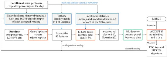
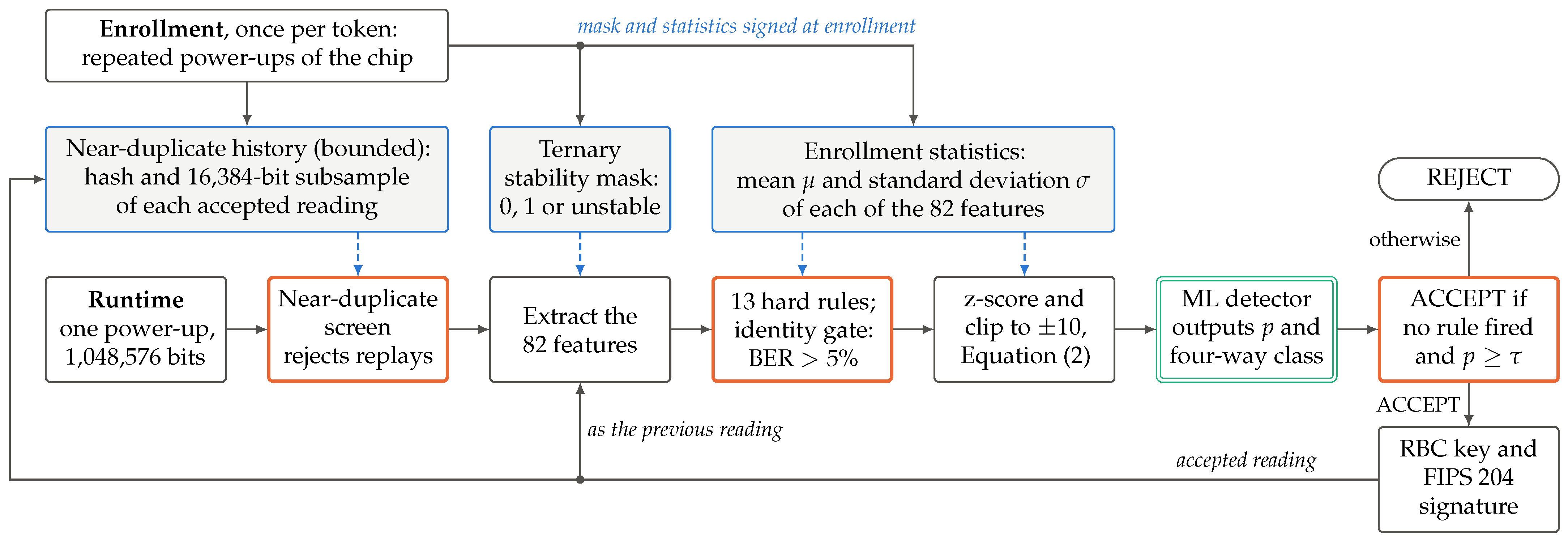
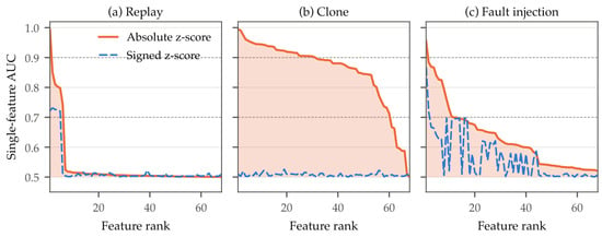
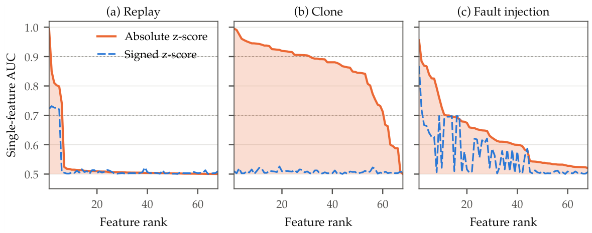
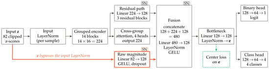
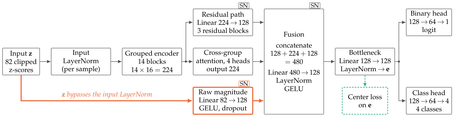
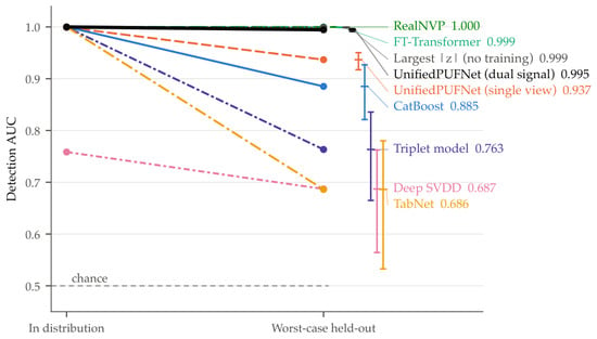
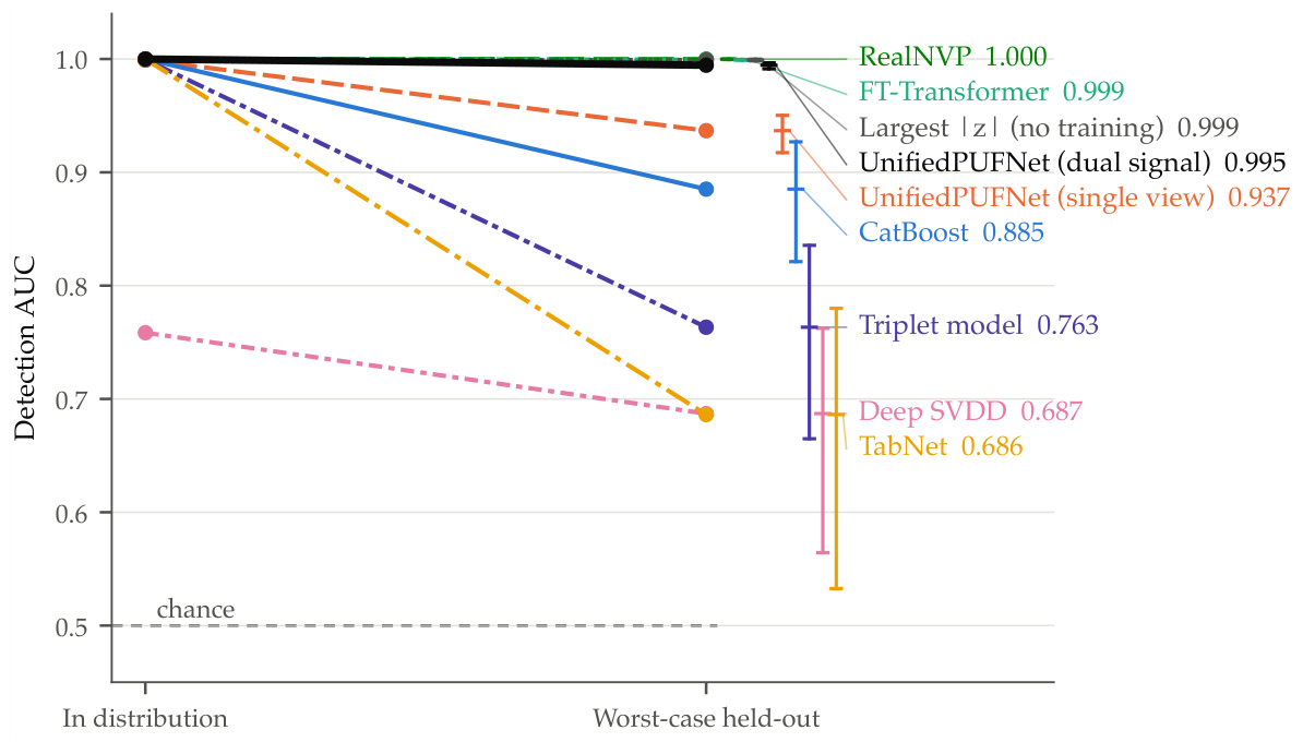
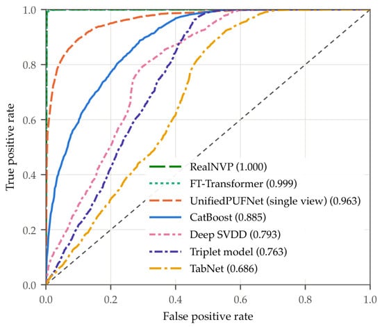
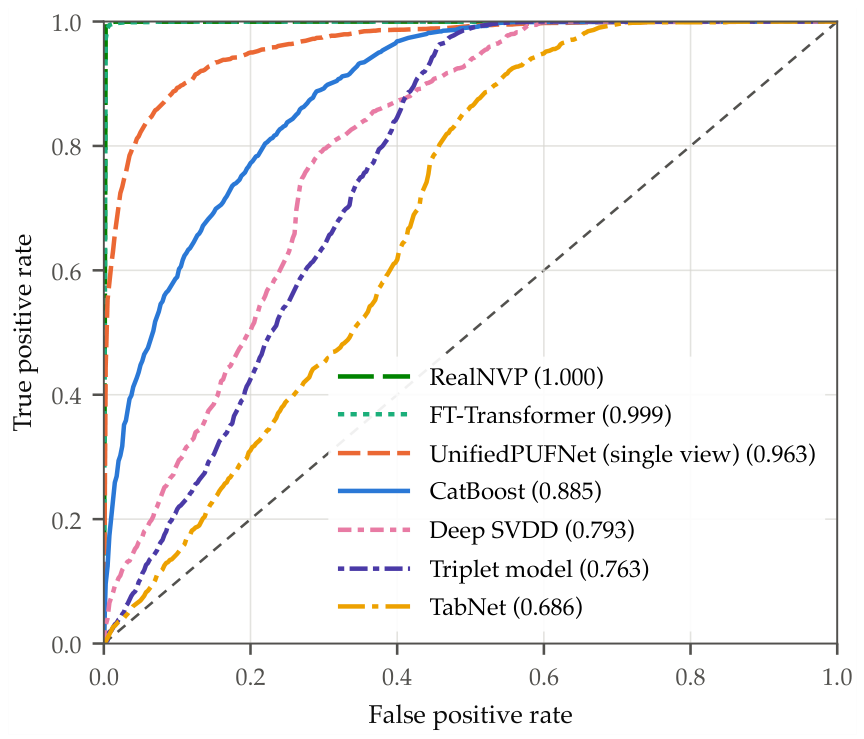
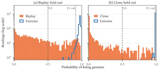
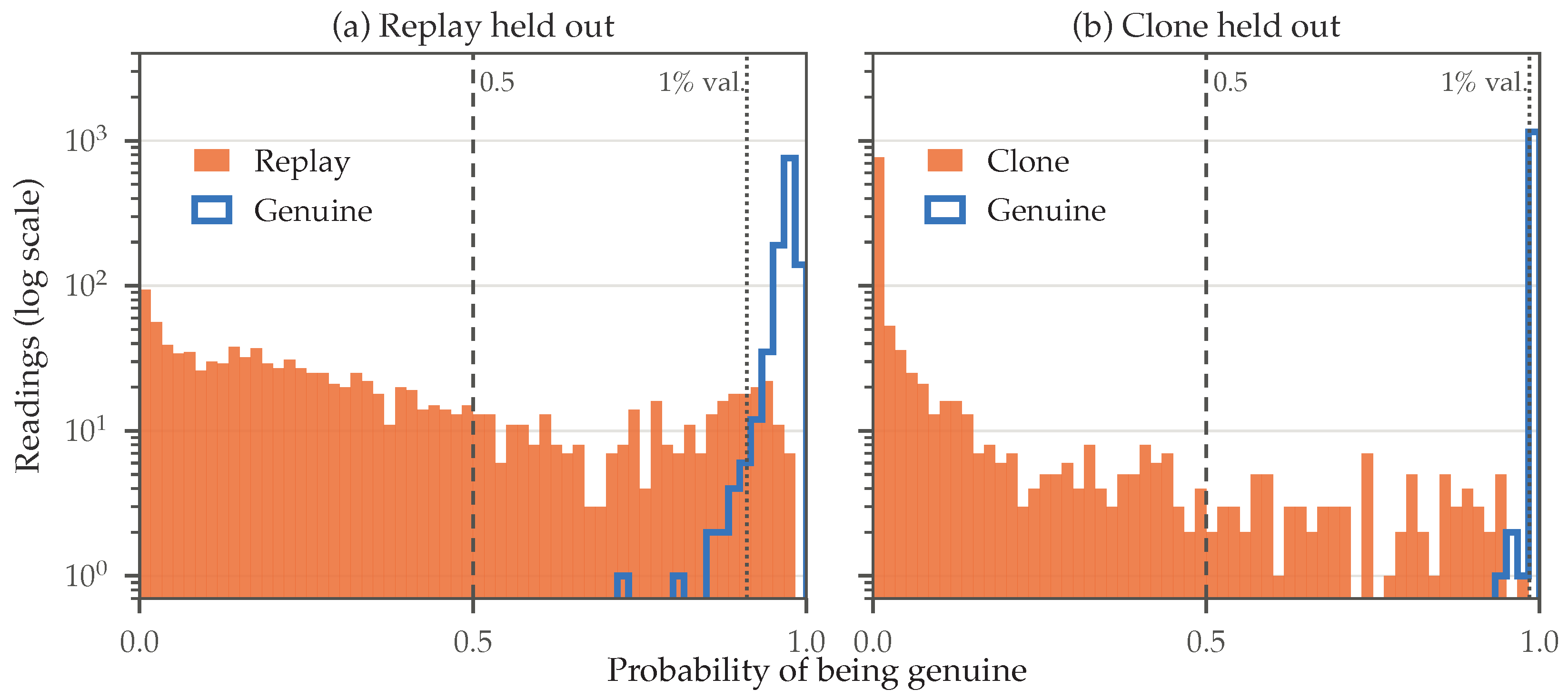
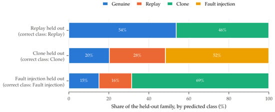
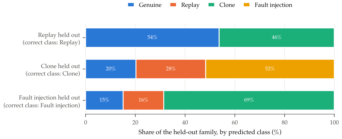
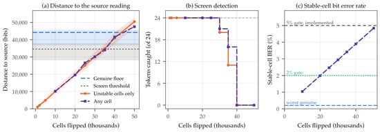
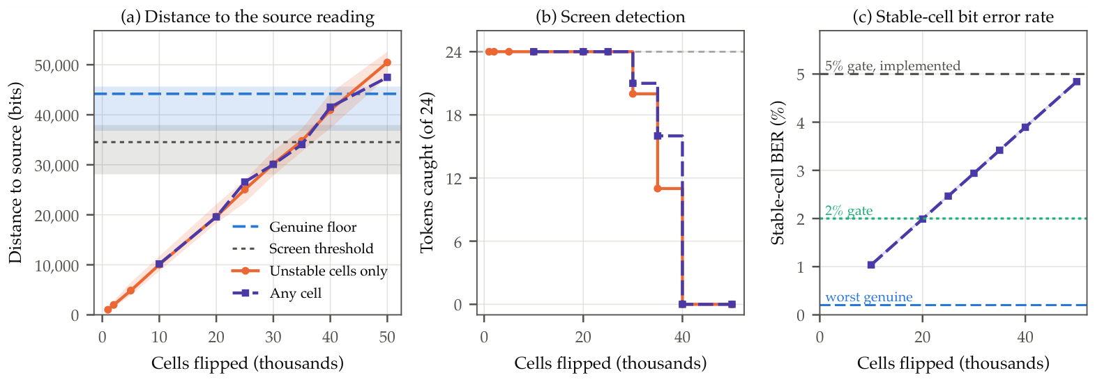

Disclaimer/Publisher’s Note: The statements, opinions and data contained in all publications are solely those of the individual author(s) and contributor(s) and not of MDPI and/or the editor(s). MDPI and/or the editor(s) disclaim responsibility for any injury to people or property resulting from any ideas, methods, instructions or products referred to in the content. |
© 2026 by the authors. Licensee MDPI, Basel, Switzerland. This article is an open access article distributed under the terms and conditions of the Creative Commons Attribution (CC BY) license.