A Multi-Graph Diffusion Mamba Framework for Ultra-Short-Term Wind Power Forecasting

Abstract

Accurate ultra-short-term wind power forecasting is critical to grid security and economic dispatch. However, existing methodologies are constrained by two fundamental gaps: rigid topologies that fail to balance physical and data-driven information, and decoupled architectures that process spatial and temporal features separately. To address these gaps, this paper proposes a novel Multi-Graph Diffusion Mamba (MGDM) framework. A multi-graph architecture is introduced to decouple the dependencies among wind turbines into a physics-informed Meteorological Causal Graph (MCG) that captures directional wind propagation, and a learnable Systemic Adaptive Graph (SAG) that encodes unobserved operational constraints. A dynamic gated fusion mechanism adaptively balances the two graphs through a real-time confidence factor, and the fused representation is finally fed into a topology-aware Mamba module, where graph diffusion convolutions are embedded into the selective scan process, achieving joint spatio-temporal modeling. The results demonstrate that the MGDM outperforms all baseline models for 15 min, 1 h, 2 h, 3 h and 4 h ahead forecasts, and achieves improvements in accuracy of 3.59–4.81% across the forecasting horizons over the best benchmark model. Moreover, ablation studies demonstrate that the multi-graph topology and the selective scan mechanism are indispensable for robust forecasting. The gating factor is further validated to serve as an indicator of regime switching, reflecting the model’s dynamic balance between physical and data-driven graphs under varying scenarios. These results confirm that the MGDM delivers consistent improvements in both forecasting accuracy and model interpretability under diverse operating conditions in the evaluated wind farm.

1. Introduction

Driven by the target of global decarbonization, wind power has become a cornerstone of sustainable power systems [1]. However, the increasing scale and clustering of wind farms have posed significant challenges for grid stability, operational efficiency, and market reliability [2,3]. To address these challenges, wind power forecasting (WPF) techniques offer a cost-effective solution and have thus become an indispensable methodology for supporting large-scale grid integration [4,5].

Conventional approaches to WPF are broadly categorized into physical and statistical methodologies [6]. Physical methods construct physics-based models from numerical weather prediction (NWP) inputs. However, they tend to oversimplify local topographic effects and wake dynamics, failing to capture the complex aerodynamics of real-world wind farms. Statistical methods, by contrast, rely on empirical correlations between historical power output and meteorological variables. While computationally efficient and robust under normal conditions, these methods often prove unreliable during extreme weather events [7,8,9].

With the advancement of intelligent technologies, approaches for WPF have evolved from traditional statistical models to data-driven deep learning paradigms. To address the non-stationarity and multi-scale fluctuations inherent in wind power sequences, researchers have combined signal processing algorithms with deep learning models [10,11,12]. To overcome the relatively coarse data resolution of numerical weather prediction (NWP), researchers encoded aerodynamic and meteorological causal priors into data-driven models [13,14,15,16]. Strategies including meteorological causal discrimination, cross-scale data correction, and time-frequency domain decoupling were employed to mitigate the dual constraints of insufficient NWP accuracy and multi-dimensional feature redundancy [17,18].

In order to overcome the limited representational capacity of single models, multi-task joint training and Mixture-of-Expert (MoE) methods have been explored. Guided by mathematical modules, Zheng et al. [19] introduced a wavelet decomposition-based adaptive MoE network, enabling stable and adaptive switching of expert weights under real-time operating conditions. Wang et al. [20] integrated a dual-path framework with financial technical indicators (FTI), where the MoE-optimized CatBoost significantly enhanced stability across diverse conditions. Li et al. [21] adopted a reinforcement learning perspective, proposing an adaptive weighted combination forecasting method that employs Deep Deterministic Policy Gradient (DDPG) as a weight generator, achieving noise-robust optimization in the forecasting process. Collectively, these studies construct a mechanism that effectively leverages the complementary advantages of multiple base learners.

Power generation in large-scale wind farms is characterized by strong spatio-temporal coupling among wind turbines and their associated meteorological variables. To model such dependencies, various graph-based approaches have been developed. Liu et al. [22] employ a hybrid “adaptive GCN + LSTM” encoder to extract fine-grained spatio-temporal features, constructing an adaptive graph by fusing a static physical adjacency graph with a learnable parameter matrix. However, the graph structure is a linear combination of the static geometric proximity matrix and the learnable matrix, which fails to capture the wind-direction-dominated asymmetric wake mechanism or reflect the causal directionality of airflow information. Wu et al. [23] replace the conventional Chebyshev approximation with an interpolation GCN to accelerate feature extraction over time-varying topologies. Nevertheless, the algorithm prevents spatial topology aggregation from propagating into the stepwise updates of temporal hidden states, leading to information fragmentation and error accumulation in multi-step recursive inference. Gao et al. [24] combine Variational Mode Decomposition (VMD) with Adaptive Local Iterative Filtering (ALIF) and introduce an adaptive graph with MixHop convolution to capture dynamic inter-variable correlations. However, the model focuses on dependencies among meteorological variables while neglecting the asymmetric aerodynamic causality induced by wake deficits and wind direction shifts. Moreover, the spatial graph aggregation and temporal state updates are performed in separate modules, which tends to cause memory decay during long-range temporal inference and makes spatio-temporal co-evolution difficult to achieve. Echeverri et al. [25] model the local wake superposition effect of multiple upstream turbines on a single downstream turbine in dense wind farms, but the topology relies entirely on a rigid static geometric graph and thus cannot cope with dynamic grid disturbances. Furthermore, the study validates only single-step forecasting (10 min), without multi-step temporal rolling inference.

In conclusion, a critical review of the existing literature reveals two persistent gaps. First, in terms of spatial topology, purely data-driven graphs lack physical boundaries and are prone to overfitting, thus misinterpreting artificial curtailments or sensor noise as spatial dependencies, while physics-informed graphs, despite encoding wind propagation priors, remain structurally fixed and fail to adapt to time-varying wind directions or unobserved grid constraints. Most existing paradigms do not incorporate a dynamic routing mechanism to balance aerodynamic causality with systemic constraints. Second, in terms of spatio-temporal modeling, mainstream approaches tend to adopt a cascaded architecture that executes spatial graph modeling and temporal sequence propagation in an alternating manner. This separation hinders spatio-temporal co-evolution, leading to error accumulation and memory decay in multi-step forecasting.

To bridge the aforementioned gaps, a novel framework named Multi-Graph Diffusion Mamba (MGDM) is proposed in this study. The framework models the spatio-temporal behaviors of wind energy through a multi-graph paradigm, achieving end-to-end cooperative power prediction for multiple wind turbines. The core contributions of this study are as follows:

(1) We propose a multi-graph framework that decouples spatio-temporal interactions into two parallel graphs. Unlike existing studies that rely on a single graph structure or a rigid geometric graph, MGDM introduces a physical-driven Meteorological Causal Graph (MCG) via transfer entropy across wind turbines and a data-driven Systemic Adaptive Graph (SAG) to learn the node embedding relationship.

(2) We design a dynamic gated fusion mechanism that generates a real-time confidence factor $\mathrm{g}\in (0,1)$, which prioritizes aerodynamic causality when $\mathrm{g}\to 1$ under stable weather conditions, and shifts to adaptive residuals when $\mathrm{g}\to 0$ during particular interventions such as active power curtailment or pitch-angle saturation, ensuring robustness against operational anomalies.

(3) We introduce a topology-aware module based on a selective scan mechanism that embeds bidirectional graph diffusion operators into the Mamba. The control matrices are dynamically driven by graph convolutions over the fused topology, enabling the simultaneous extraction of temporal and spatial information. Rather than following the conventional cascade of alternately stacked graph convolution and temporal attention modules, MGDM natively embeds a bidirectional graph diffusion operator into the continuous discretization control matrix of the Mamba state space, achieving true stepwise co-evolution between node spatial diffusion and temporal hidden state updates.

(4) We adopt a physics-informed loss function that couples a robust task loss with a structural regularization term. This term penalizes the Frobenius norm divergence between the two graphs. Evaluated on a real-world multi-turbine dataset, our framework consistently outperforms State-of-the-Art benchmarks across multi-step forecasting horizons. What is more, the proposed method avoids the quadratic complexity and excessive stacking of Transformer attention, while overcoming memory decay and error accumulation in power forecasting tasks at strictly linear complexity and a compact parameter count.

The remainder of this paper is organized as follows. Section 2 describes the wind power dataset and provides a spatio-temporal correlation analysis. Section 3 presents the theoretical foundations and forecasting architecture of the Multi-Graph Diffusion Mamba. Section 4 conducts comparative experiments and ablation studies, evaluates the model’s forecasting performance, and validates its robustness and physical interpretability. Finally, Section 5 summarizes the paper and provides an outlook on future research directions.

2. Analysis of Wind Power Data

This section analyzes the wind power data from three perspectives: dataset description, spatio-temporal correlation analysis, and adaptive decomposition. Transfer entropy is used to capture causal interactions among turbines, revealing seasonal variations and identifying wake-affected downstream sites. Empirical Wavelet Transform (EWT) further extracts localized frequency components from the non-stationary power sequences for subsequent forecasting.

2.1. Dataset

This study utilizes historical operational data collected from four wind turbines (designated as FD1-FD4) located at an onshore wind farm in China. The dataset spans from 1 January 2019 to 31 December 2020, featuring a 15 min temporal resolution. The raw data comprise power outputs and multi-height meteorological variables, including wind speed, wind direction, ambient pressure, temperature, and relative humidity. Raw industrial SCADA measurements are inevitably corrupted by sensor malfunctions, network latency, and scheduled maintenance. A sequential data-cleansing protocol was therefore applied based on physical turbine limits: (i) out-of-bound values (e.g., negative power, wind speed outside 0–45 m/s, or pressure outside 900–1050 hPa) were marked invalid and negative power was reset to 0 kW; and (ii) stuck sensors were identified as constant telemetry over more than four consecutive intervals. After implementing data preprocessing and anomaly removal, the final dataset yielded 55,442, 58,769, 58,079, and 56,993 effective 15 min samples for turbines FD1 to FD4, respectively. A temporal inner-join synchronization was performed across all four turbines. Only timestamps where all four units possessed simultaneous, valid observations were retained, yielding exactly 51,031 synchronized multi-node snapshots.

The wind turbines exhibit a cut-in speed of 3.5 m/s and reach rated saturation power at 16 m/s. According to the Beaufort wind scale, extreme gale weather is defined in this study as a 10 min average wind speed at a 70 m hub height exceeding 17.2 m/s (≥Force 8). Model inputs comprise historical power data and selected meteorological parameters detailed in Table 1. The two-year dataset is partitioned into eight distinct subsets corresponding to the four seasons. The synchronized chronological sequence was partitioned by calendar season across the two-year span: Spring (March–May), Summer (June–August), Autumn (September–November), and winter (December–February). For each seasonal subset, the continuous timeline was split strictly chronologically into training, validation, and testing sets using a 70%:15%:15% ratio without random shuffling. To ensure maximum operational generalization and eliminate multi-model maintenance overhead, a single unified MGDM model was trained across the training partitions and subsequently evaluated across the distinct seasonal test sets. All continuous feature channels were scaled into the interval [0, 1] using Min-Max normalization.

Table 1. Summary of the wind power and meteorological variables.

Input Variables	Range
Power (kW)	(0, 100)
Wind speed at 70 m (m/s)	(0, 20)
Wind direction at 70 m (°)	(0, 360)
Ambient Temperature (°C)	(−15, 40)
Ambient Pressure (hPa)	(950, 1020)
Ambient Humidity (%)	(0, 100)

2.2. Spatio-Temporal Correlation Analysis

Conventional graph construction methods for spatio-temporal correlation analysis often rely on restrictive assumptions, such as spatial homogeneity and undirected linear correlations. These approaches fail to capture the directed, nonlinear information flows inherent in wind farm dynamics. To address this, we propose a novel graph construction framework grounded in causality and information theory, which maps directed information flow rather than static spatial similarity.

Transfer entropy quantifies the directed information flow and the causal influence exerted by the historical state on the current state [26,27]. For two sequences denoted as $\mathit{X}\left(x_t\right)$ and $\mathit{Y}\left(y_t\right)$, the transfer entropy from $\mathit{X}$ to $\mathit{Y}$ is defined as Equation (1).

$$\begin{array}{c}\begin{array}{c}T{E}_{\mathit{X}\mathit{Y}}=TE\left({\mathit{Y}}_{t+1}\mid {\mathit{Y}}_t,{\mathit{X}}_t\right)-TE\left({\mathit{Y}}_{t+1}\mid {\mathit{Y}}_t\right)\\ =\sum p\left(y_{t+1},y_t^{\left(l\right)},x_t^{\left(m\right)}\right){\mathit{log}}_{2}p\left(y_{t+1}{y}_t^{\left(l\right)},x_t^{\left(m\right)}\right)-\sum p\left(y_{t+1},y_t^{\left(l\right)}\right){\mathit{log}}_{2}p\left(y_{t+1}\mid y_t^{\left(l\right)}\right)\end{array}\end{array}$$

(1)

where $TE\left({\mathit{Y}}_{\mathrm{t}+1}\mid {\mathit{Y}}_{\mathrm{t}},{\mathit{X}}_{\mathrm{t}}\right)$ represents the conditional entropy of $\mathrm{Y}$ at the subsequent time step given the historical states of both $\mathrm{X}$ and $\mathrm{Y}$. Correspondingly, $TE\left({\mathit{Y}}_{\mathrm{t}+1}\mid {\mathit{Y}}_{\mathrm{t}}\right)$ signifies the conditional entropy of ${\mathit{Y}}_{\mathrm{t}+1}$ given solely its own historical trajectory. $\mathrm{l}$ and $\mathrm{m}$ denote the historical length for the target and source sequences, respectively, and $\mathrm{p}(\cdot )$ denotes the probability computation.

Transfer entropy is advantageous for wind power modeling due to the following properties: (1) its asymmetry provides inherent directionality, distinguishing causal drivers from responses; (2) it captures complex nonlinear interactions, such as wake effects; (3) its distribution-based formulation avoids parametric assumptions, making it suitable for non-stationary signals; and (4) it supports time-lag analysis, enabling the detection of delayed wind propagation across turbines.

To dynamically capture the non-stationary correlations across wind turbines, a 30-day sliding window (sample size N = 2880) is implemented. When computing transfer entropy, the binning parameter (denoted as B) is required to satisfy the inequality N > B³ that the sample size should be large enough to support the three-dimensional joint probability distribution. For any forecast issued at time point t, transfer entropy is computed under strict temporal causality, using only backward-looking data over the preceding N intervals, defined over the historical window [t − N + 1, t]. In order to balance numerical stability with accurate probability estimation, we set history lengths k = l, time lag = 1 sample, discretization into B = 13 bins determined from the training set, with Laplace smoothing for the 3D joint probability estimation.

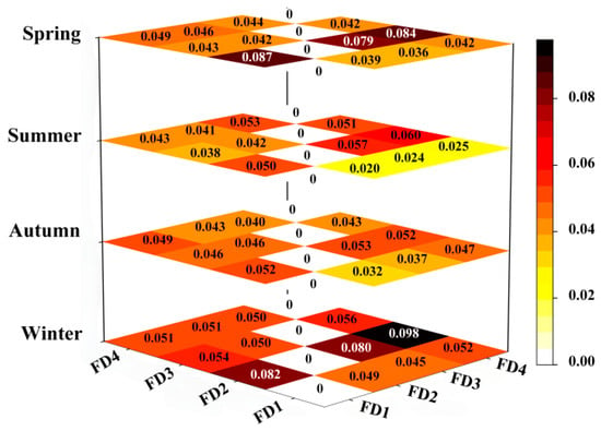
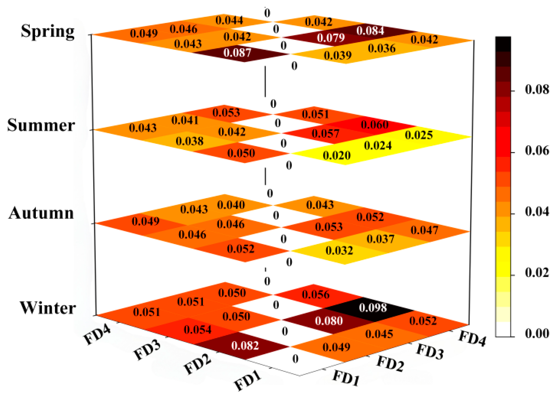
Figure 1 illustrates the seasonally averaged transfer entropy among wind turbines, revealing pronounced seasonal variations in the four sites. Among transfer entropy matrices, the second column (i.e., $T{E}_{\mathrm{o}\mathrm{t}\mathrm{h}\mathrm{e}\mathrm{r}\mathrm{s}\to \mathrm{F}\mathrm{D}2}$) consistently maintains the highest level, while the second row is relatively weak, reflecting that FD2 is aerodynamically a typical downstream site or wake convergence point.

Figure 1. Heatmap of seasonal transfer entropy matrices for the four wind turbines. Darker colors indicate stronger causal influence.

Due to local prevailing wind patterns, non-prevailing directional sectors inevitably suffer from limited observations. To circumvent numerical zero-frequency singularities in 3D joint probability estimation, Laplace (add-one) Dirichlet smoothing is incorporated into the probability tensor. For extremely sparse sectors where valid samples fall below an empirical statistical threshold (N_s < 500), the causal adjacency matrix automatically reverts to an inverse-distance physical prior.

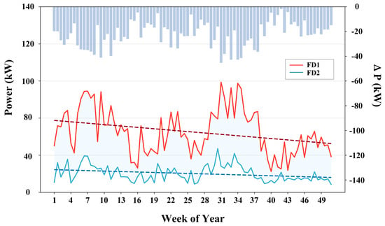
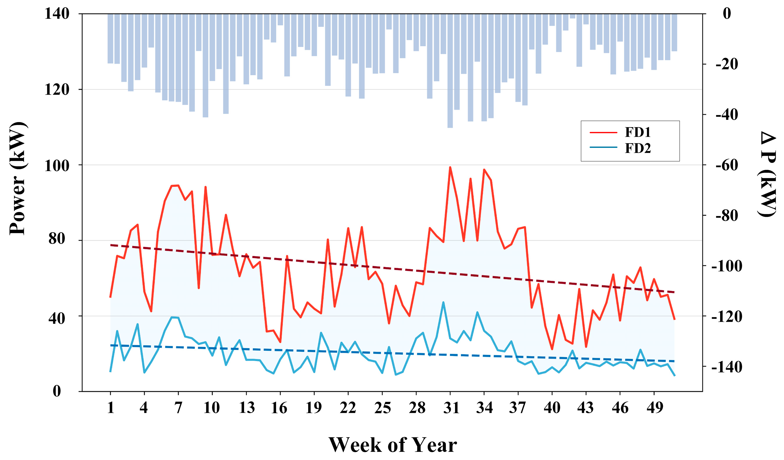
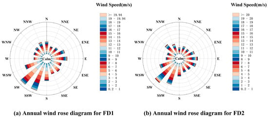
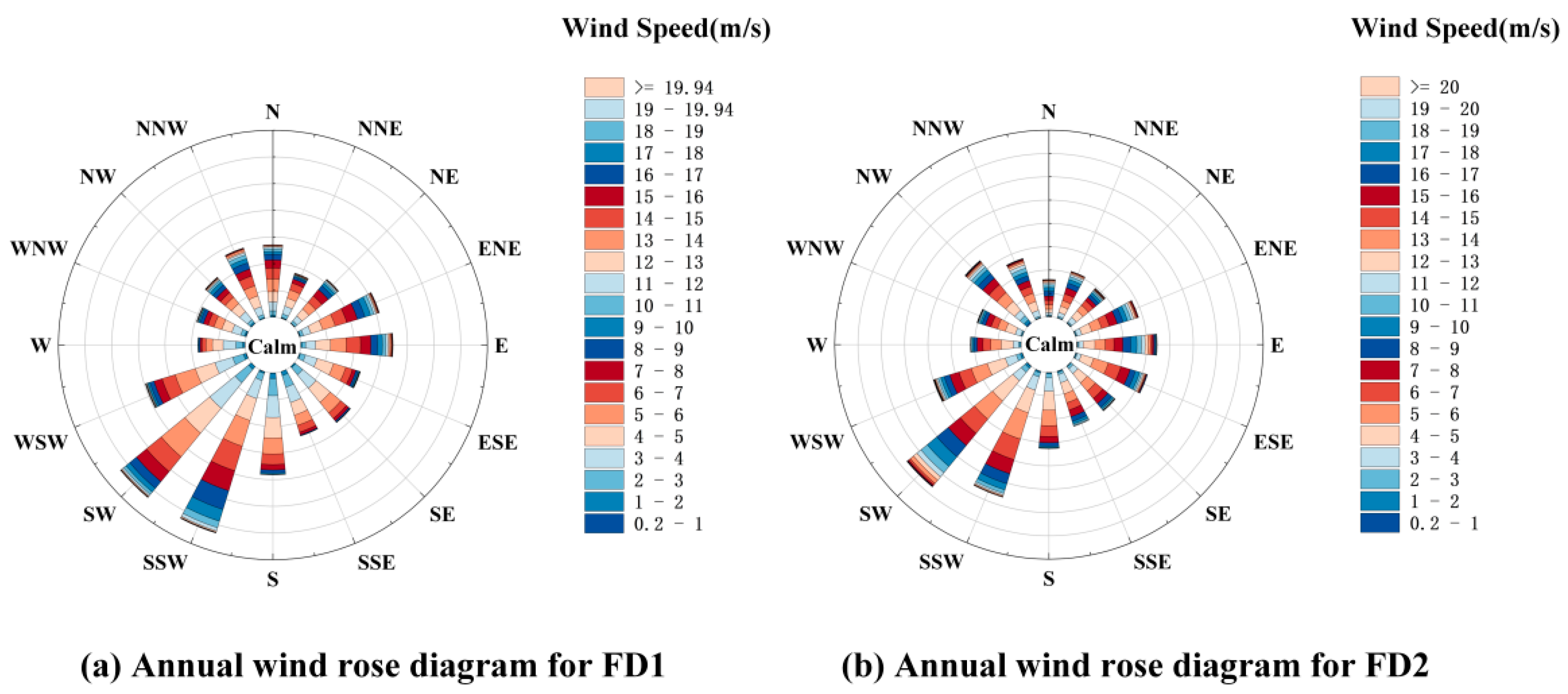
Taking FD1 and FD2 as an example, Figure 2 illustrates the weekly average power generation in 2019. The power curves of the two turbines exhibit a structural bias, and the inverted bar chart at the top quantifies the power difference $\mathsf{\Delta }\mathrm{P}={\mathrm{P}}_{\mathrm{F}\mathrm{D}2}-{\mathrm{P}}_{\mathrm{F}\mathrm{D}1}$, which remains in the negative range throughout the year. Figure 3 presents the annual wind rose diagrams for FD1 and FD2. The prevailing wind directions for both turbines are concentrated in the south-southwest (SSW) to southwest (SW) sector. Compared with FD1, FD2 exhibits a significantly lower proportion of high wind speed intervals (e.g., exceeding 14 m/s, represented by warm-colored bands) within the prevailing sector, indicating that FD2 operates predominantly in the downstream position of the wind farm.

Figure 2. Weekly average wind speeds and output power comparison between FD1 and FD2 in 2019. The upper bar chart illustrates the power differential ($\mathsf{\Delta }\mathrm{P}={\mathrm{P}}_{\mathrm{F}\mathrm{D}2}-{\mathrm{P}}_{\mathrm{F}\mathrm{D}1}$).

Figure 3. Annual wind rose comparisons for FD1 and FD2. (a) FD1 and (b) FD2. FD2 shows a reduced frequency of high-speed events (>14 m/s, in warm colors) within this sector, consistent with a downstream turbine location.

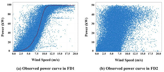
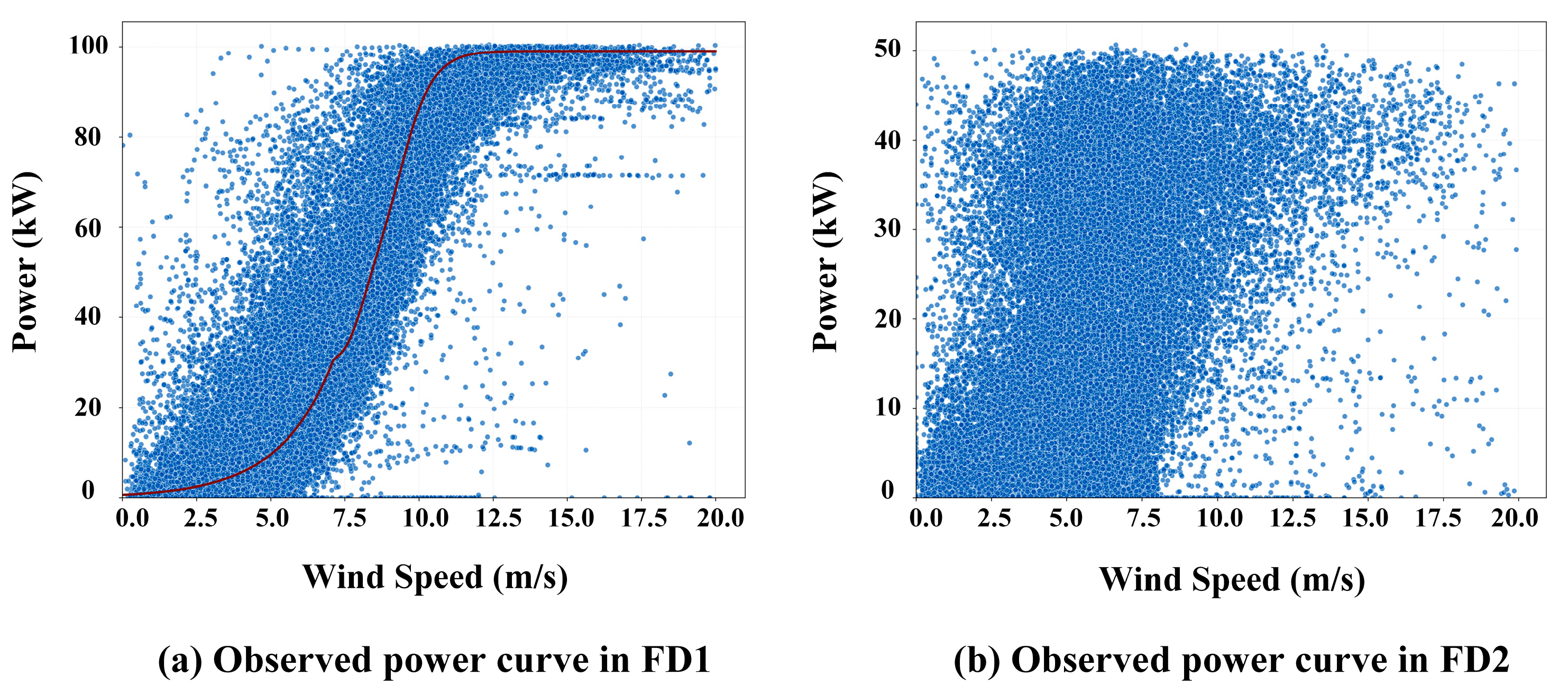
Figure 4 shows the wind speed–power scatter plots for FD1 and FD2. Under normal conditions, once the cut-in wind speed is exceeded, the output power increases approximately following a cubic relationship with wind speed. After the saturation point, the power stabilizes, as shown in Figure 4a. In contrast, the data for FD2 exhibit a considerably higher degree of dispersion, mainly attributable to complex inflow conditions from upstream turbine wakes, as shown in Figure 4b, making it difficult to identify a clear inflection point. Moreover, the output power of FD2 is degraded by high turbulence intensity and wake deficits, which corroborates the results of transfer entropy analysis.

Figure 4. Wind speed–power scatter plots for FD1 and FD2. (a) Raw observed data with a red fitting line in FD1. (b) Raw observed data in FD2.

Considering the large sample size and limited computational resource, this study does not perform rigorous surrogate data testing on the significance level of each matrix. Instead, we directly feed the raw dynamic transfer entropy matrices to the subsequent model. During backpropagation, the model can automatically assign higher attention weights to strong causal edges, thereby achieving end-to-end topology learning.

2.3. Adaptive Decomposition of Wind Power Sequences

The data of output power constitutes highly non-stationary, non-linear time series driven by coupled physical mechanisms [28]. To capture the localized characteristics of wind power sequences, we employ the Empirical Wavelet Transform (EWT) to adaptively decompose the raw signal into distinct components. The rolling EWT uses a stride of one sample (15 min); a new 7-day window is generated at every forecast origin, yielding distinct sub-modes and a residual for each interval. The corresponding modes across all windows are then concatenated chronologically, followed by a weighted-average fusion applied within the overlapping regions to mitigate boundary discontinuities. Frequency-band boundary selection. Band boundaries are determined by detecting local maxima of the Fourier spectrum and using midpoints between consecutive maxima, following the original EWT formulation. The hyperparameter configuration for the EWT sets four modes, a penalty factor of 1000, and a convergence tolerance of 10⁻⁶. Mirror padding is applied at both window ends before the Fourier transform, and the extended region is discarded after reconstruction.

To satisfy real-world deployment constraints, the rolling EWT decomposition is implemented causally and retrospectively. At any target forecast point t, the sliding window covers only the historical interval [t − 671, t], i.e., exactly 7 days of SCADA telemetry. At boundary transitions across chronological splits (e.g., from validation to test), the rolling window may include historical observations preceding the test partition, but only as look-back conditioning inputs. All decomposition reconstruction metrics and downstream loss gradients are computed exclusively on target predictions within the test partition, and the boundary weighted-average fusion matrix operates only over overlapping historical intervals up to time t.

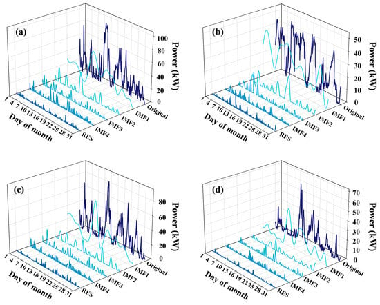
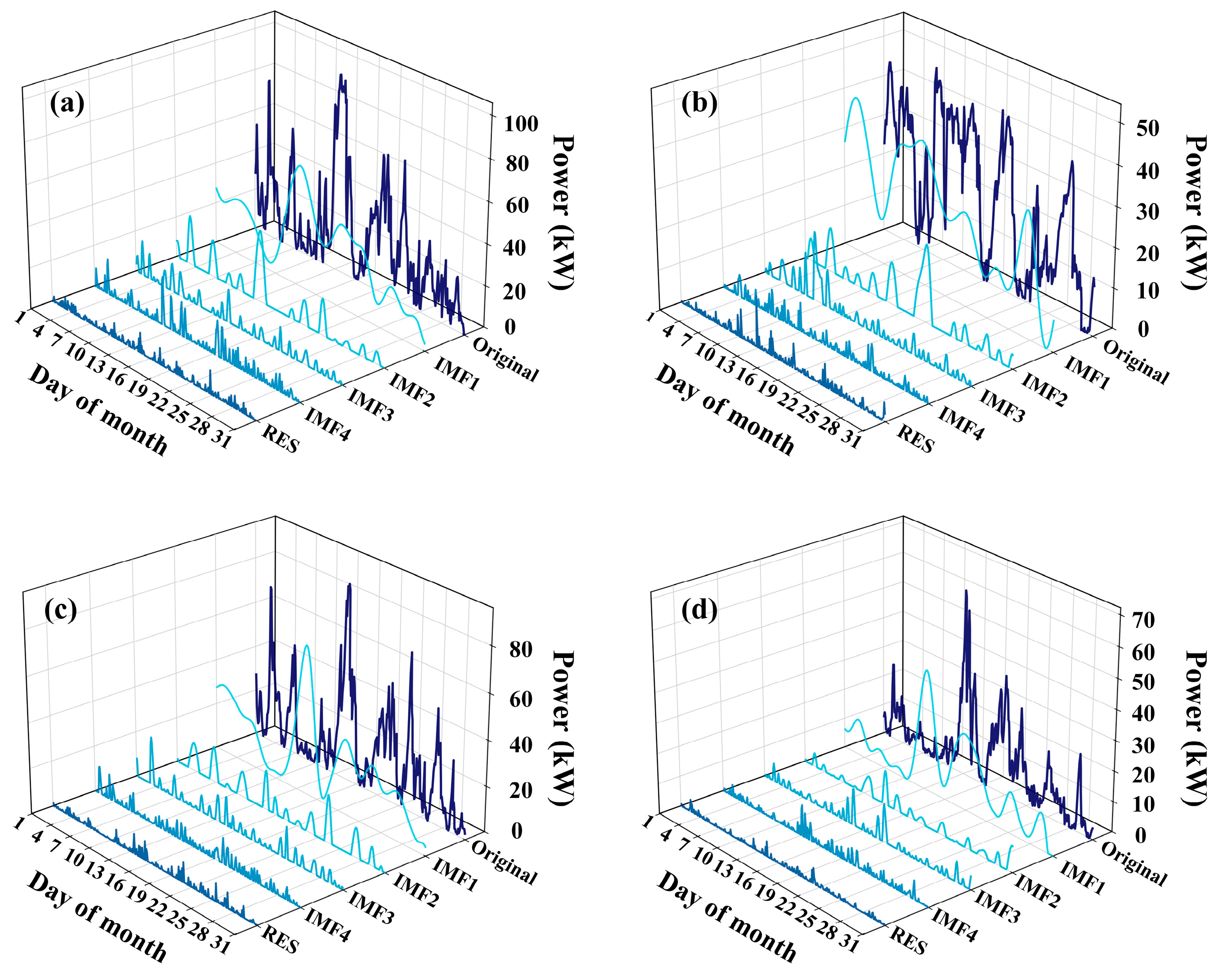
Figure 5 illustrates the EWT results for the data of January 2019. The decomposition yields a set of modes arranged in ascending order of frequency, which are well-separated with negligible mode mixing.

Figure 5. Decomposition results of the EWT algorithm for the four wind turbines in the window of January 2019. (a) FD1. (b) FD2. (c) FD3. (d) FD4.

To guarantee strict chronological causality and eliminate look-ahead leakage, all preprocessing parameters were fitted exclusively on the training partition. Specifically, Min-Max normalization extrema were calibrated solely on training data and frozen before scaling the validation and test sequences. To avoid cross-partition boundary contamination from sliding windows, a chronological buffer equal to the maximum window length was utilized (30 days for transfer entropy, 7 days for EWT). Validation and test evaluation targets are restricted to time steps that lie strictly within the test partition, ensuring that no future-partition observations participate in model parameterization or feature extraction.

3. Methodology

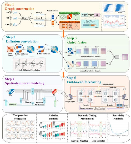
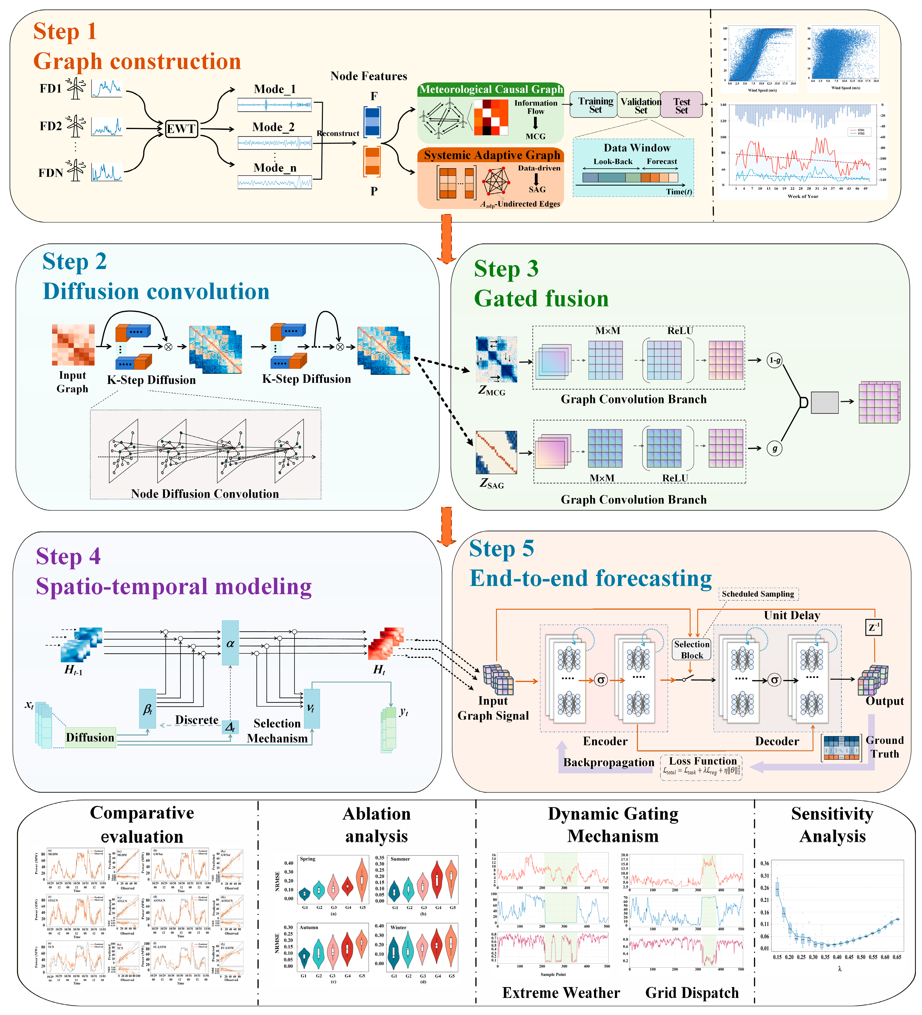
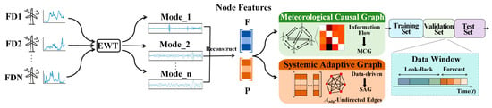
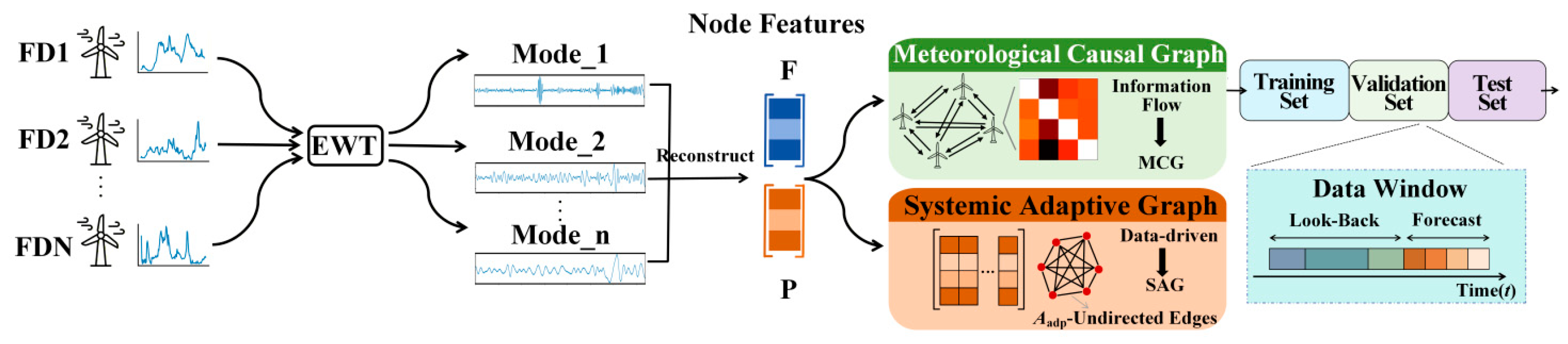
In this study, we propose a novel framework named Multi-Graph Diffusion Mamba (MGDM) for spatio-temporal dependency modeling in the wind farm, as depicted in Figure 6. We construct a Meteorological Causal Graph (MCG) using transfer entropy to capture directional wind propagation, and a learnable Systemic Adaptive Graph (SAG) to model unobserved operational constraints. Graph diffusion convolution extracts spatial dependencies from both topologies, while a dynamic gated fusion mechanism adaptively balances their contributions under varying conditions. The fused representation is integrated into a Mamba-based selective scanning backbone with topology-aware convolutions, enabling simultaneous spatial aggregation and temporal state updates for joint modeling of coupled dynamics. The model is trained end-to-end with a physics-informed loss function.

Figure 6. Flow chart of the proposed methodology.

3.1. Multi-Graph for Spatio-Temporal Dependency Modeling

A graph representation of multi-turbine data enables the modeling of spatial dependencies, as exhibited in Figure 7. In a graph, each turbine is abstracted as a node, and the edges encode the spatial dependencies among the units. Given a graph $\mathit{G}=(\mathit{V},\mathit{E},\mathit{A})$, where $\mathit{V}=\{{\mathit{v}}_1,\dots ,{\mathit{v}}_{\mathrm{N}}\}$ denotes the set of nodes, $\mathit{E}={\{\mathit{e}}_{\mathrm{i}\mathrm{j}},\mathrm{i},\mathrm{j}\in N\}$ is the set of edges, A represents the adjacency matrix, and $N$ is the number of nodes. To reduce redundant information, the data collected from the N turbines are transformed using EWT, yielding node-specific feature $\mathrm{F}$, where each element is reconstructed from the first four decomposition sequences respectively. Similarly, the historical power data is obtained as $\mathrm{P}$ (Equation (2)). Thus, the wind power forecasting model can be formulated as Equation (2).

$$P_{t:(t+T_1)}=\Phi \left(P_{(t-T_0+1):t},F_{(t-T_0+1):t},G\right)$$

(2)

where ${\mathrm{P}}_{\mathrm{t}:(\mathrm{t}+{\mathrm{T}}_1)}$ denotes the predicted power values from time step $\mathrm{t}$ to ${\mathrm{t}+\mathrm{T}}_1$, ${\mathrm{P}}_{(\mathrm{t}-{\mathrm{T}}_0+1):\mathrm{t}}$ and ${\mathrm{F}}_{(\mathrm{t}-{\mathrm{T}}_0+1):\mathrm{t}}$ represent the historical power output and feature variables over the past ${\mathrm{T}}_0$ time steps, and $\mathsf{\Phi }(\cdot )$ denotes the target mapping function.

Figure 7. Schematic of the proposed multi-graph construction. The Meteorological Causal Graph (MCG) is built via transfer entropy to capture directional wind propagation, and the Systemic Adaptive Graph (SAG) is learned from data to encode unobserved operational constraints.

Typically, conventional approaches represent wind turbine relationships as a single topology, derived from physical proximity or data correlations. However, these methods fail to account for two distinct interaction mechanisms: (1) Meteorological mechanism: Wind propagation is directional and asymmetric, and the relationship between output power and wind-related variables is governed by physical laws. (2) Operational constraints: Factors such as grid dispatch, measurement errors, and extreme weather conditions introduce additional variability that is not captured by purely meteorological models.

In light of this, we introduce two branches: a Meteorological Causal Graph (MCG), and a latent Systemic Adaptive Graph (SAG). In the MCG, transfer entropy is used to characterize the adjacency matrix of the graph, denoted as ${\mathit{A}}_{\mathrm{M}\mathrm{C}\mathrm{G}}=\{T{E}_{\mathrm{i}\mathrm{j}},\mathrm{i},\mathrm{j}\in \mathrm{N}\}$. We partition the global wind direction into S discrete state spaces. For each state s, an independent causal matrix is computed using the data slices corresponding to specific wind direction. During forward propagation, the physical adjacency matrix is dynamically routed according to the real-time wind direction vector ${\mathrm{d}}_{\mathrm{t}}$, as presented in Equation (3).

$${\mathit{A}}_{MCG}(t)={\displaystyle \sum _{s=1}^S}\mathbb{I}\left(d_t\in D_s\right)\cdot {\mathit{A}}_{MCG}^{\left(s\right)}(t)$$

(3)

where $\mathbb{I}(\cdot )$ is the indicator function, and ${\mathrm{D}}_{\mathrm{s}}$ denotes the angular boundary of the s-th wind direction sector. The directional causal matrices ${\mathit{A}}_{\mathrm{M}\mathrm{C}\mathrm{G}}\left(\mathrm{t}\right)$ for the S wind direction sectors are parameterized as a static prior topology dictionary estimated solely from the training set. At validation and test time, the model performs a single $O\left(1\right)$ directional lookup indexed by the real-time wind direction $d_{\mathrm{t}}$ at the forecast origin.

Although MCG captures the information flow among nodes, the power generation is simultaneously influenced by other factors difficult to observe, such as extreme weather events, measurement errors and active power curtailment caused by grid dispatch. To capture these implicit systemic couplings, we introduce the SAG. A learnable node embedding matrix is defined as $\mathit{U}\in {\mathbb{R}}^{\mathrm{N}\times \mathrm{d}\mathrm{i}{\mathrm{m}}_{\mathrm{u}}}$, where $\mathrm{d}\mathrm{i}{\mathrm{m}}_{\mathrm{u}}$ denotes the embedding dimension, and each row vector ${\mathit{u}}_{\mathrm{i}}\in {\mathbb{R}}^{{\mathrm{d}\mathrm{i}\mathrm{m}}_{\mathrm{u}}}$ serves as a learnable continuous representation of the i-th node in a high-dimensional space. The adaptive adjacency matrix computes the latent spatial correlation between two turbines via the inner product, as expressed in Equation (4).

$${\mathit{A}}_{SAG}\left(t\right)=Softmax\left(ReLU\left({\mathit{U}\mathit{U}}^T\right)\right)$$

(4)

3.2. Graph Diffusion

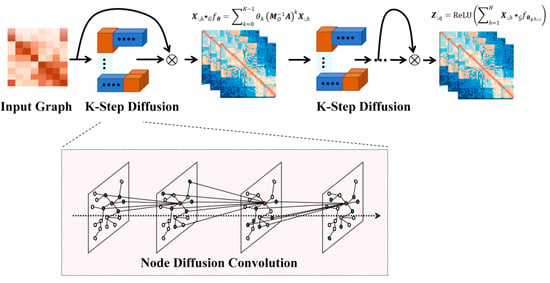
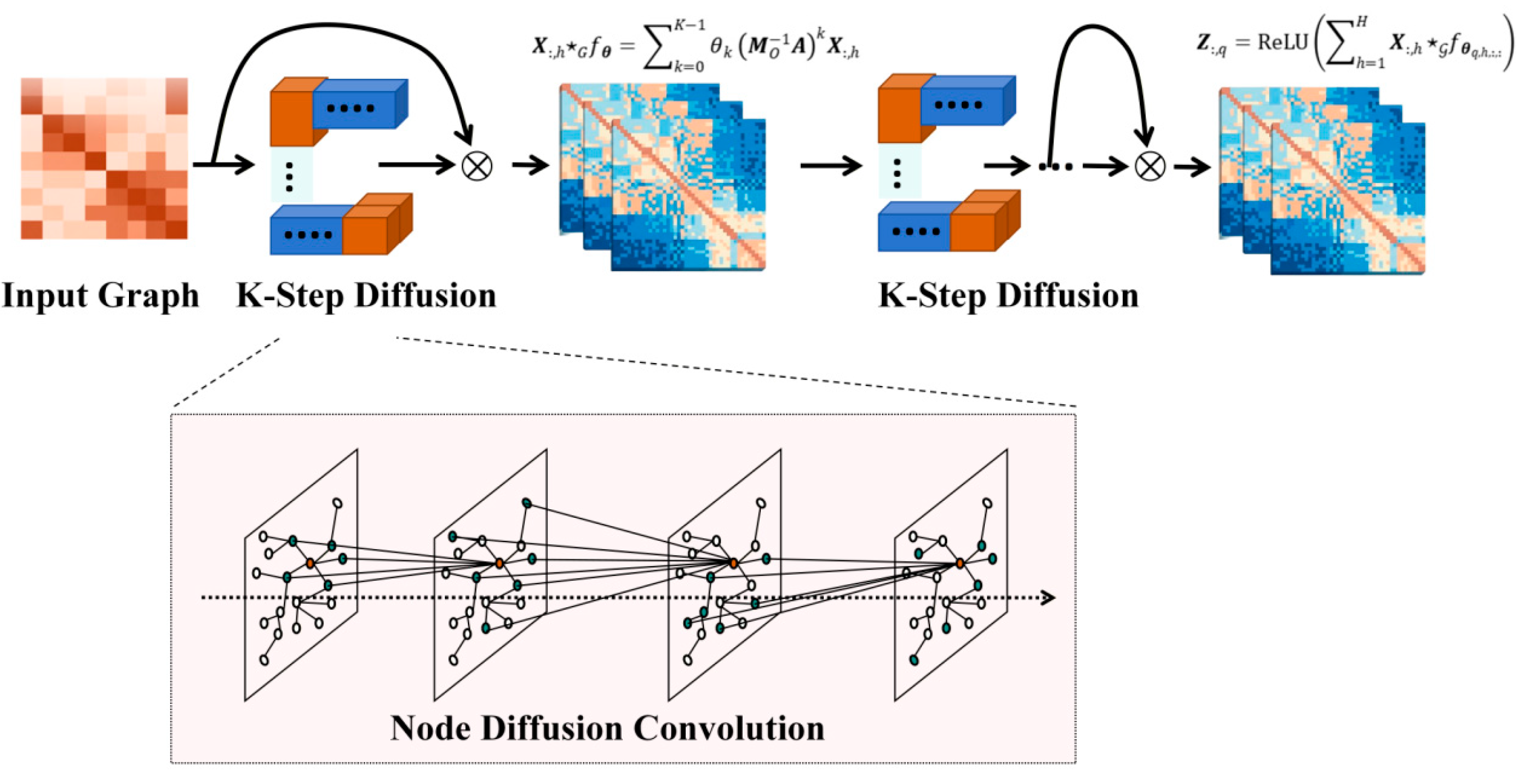
The information flow among wind turbines can be modeled as a diffusion process [29] on a graph, as illustrated in Figure 8. Assuming the restart probability is $ϵ$, and the out-degree and in-degree matrices are denoted as ${\mathit{M}}_o$ and ${\mathit{M}}_i$, respectively. The steady-state distribution of the diffusion process is given in Equations (5)–(7).

$$\begin{array}{c}{p}_{diff}={\sum }_{k=0}^{\infty }ϵ(1-ϵ{)}^k{\left({\mathit{M}}_O^{-1}\mathit{A}\right)}^k\end{array}$$

(5)

$$\begin{array}{c}{\mathit{M}}_o=diag\left(AI\right)\end{array}$$

(6)

$$\begin{array}{c}{\mathit{M}}_i=diag\left({\mathit{A}}^{T}I\right)\end{array}$$

(7)

where k is the number of diffusion steps, and $I$ denotes the matrix of all ones. We truncate the process to K steps and use bidirectional diffusion convolution to aggregate upstream and downstream information.

Figure 8. Graph diffusion convolution architecture. Through graph diffusion, the model extracts bidirectional information flow between upstream and downstream wind turbines within each time window.

For an input graph signal $\mathit{X}\in {\mathbb{R}}^{N\times R}$, the diffusion convolution is defined in Equation (8).

$$\begin{array}{c}{\mathit{X}}_{:,r}{\star }_G{f}_{\theta }={\sum }_{k=0}^{K-1}\left({\theta }_{k,1}{\left({\mathit{M}}_o^{-1}\mathit{A}\right)}^k+{\theta }_{k,2}{\left({\mathit{M}}_i^{-1}{\mathit{A}}^{\top }\right)}^k\right){\mathit{X}}_{:,r}\end{array}$$

(8)

where ${\theta }_{k,1}$ and ${\theta }_{k,2}$ are the parameters of the filter $f_{\theta }$, and $r\in \{1,\dots ,R\}$.

Based on Equation (8), we construct a diffusion convolutional layer that maps the input feature and historical power data into an output space of specified dimension. For the graph of SAG, which is undirected, a single-direction K-step diffusion is applied, and the diffusion convolution can be simplified as Equation (9):

$$\begin{array}{c}{\mathit{X}}_{:,r}{\star }_G{f}_{\theta }={\sum }_{k=0}^{K-1}{\theta }_k{\left({\mathit{M}}_O^{-1}\mathit{A}\right)}^k{\mathit{X}}_{:,r}\end{array}$$

(9)

where ${\theta }_{k,1}={\theta }_{k,2}={\theta }_k$.

Assuming the parameter space is $\theta \in {\mathbb{R}}^{Q\times R\times K\times 2}$, the convolutional layer can be expressed as Equation (10):

$$\begin{array}{c}{\mathit{Z}}_{:,q}=ReLU\left({\sum }_{r=1}^R{\mathit{X}}_{:,r}{\star }_{\mathcal{G}}{f}_{{\theta }_{q,h,:,:}}\right)\end{array}$$

(10)

where $\mathit{Z}\in {\mathbb{R}}^{N\times Q}$ is the output tensor of the diffusion convolutional layer, and $q\in \{1,\dots ,Q\}$.

The outputs of the MCG and the SAG are denoted as ${\mathit{Z}}_{phy}$ and ${\mathit{Z}}_{adp}$, respectively. Through the diffusion process, the model can extract the information flow between upstream and downstream turbines within each time window, capturing spatial dependencies in non-Euclidean space.

3.3. Dynamic Gated Fusion

The relative dominance of the two topologies is highly time-variant. A static fusion strategy cannot address the non-stationarity of real-world power systems. Therefore, we introduce a state-aware dynamic gated fusion mechanism to adaptively fuse the isomorphic features from the graph topological spaces.

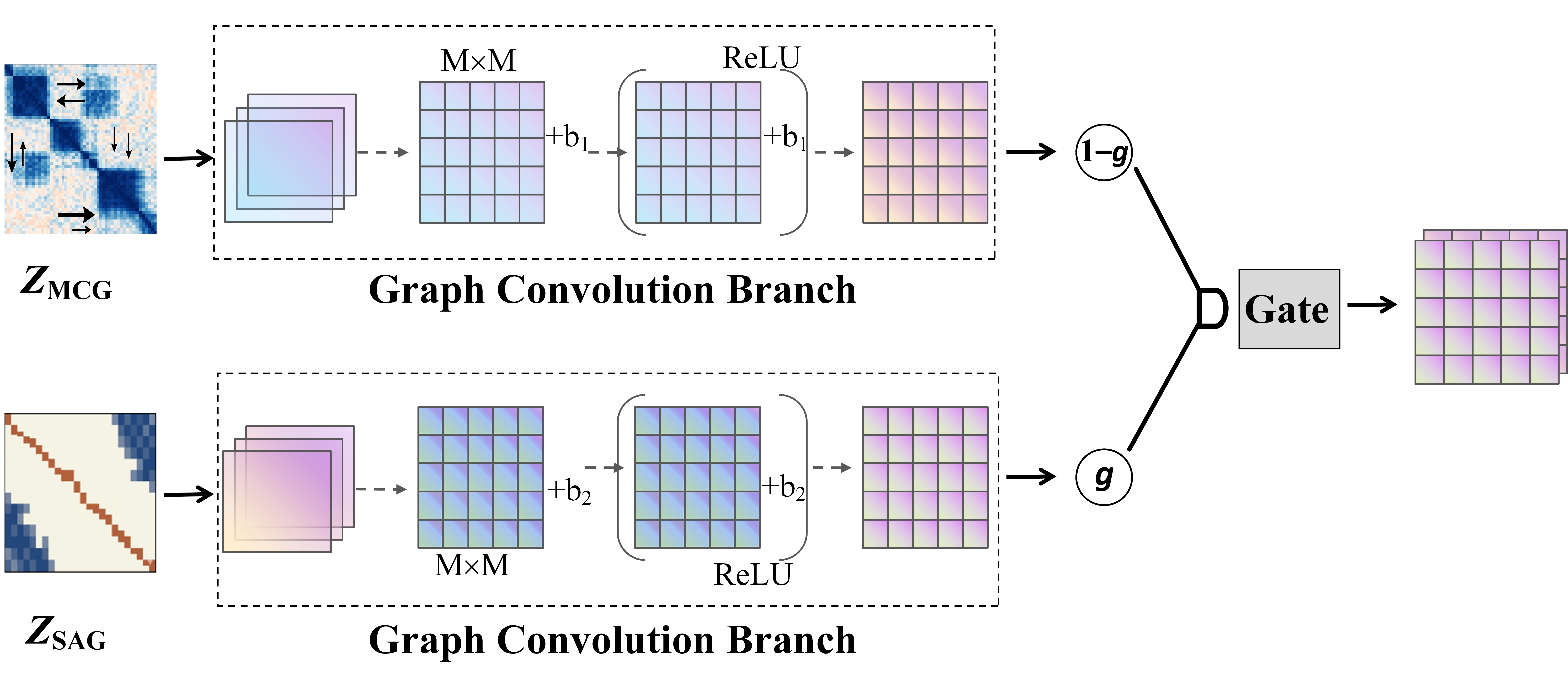
To evaluate the instantaneous reliability of each branch, we concatenate the features and project them through a non-linear mapping to synthesize a dynamic weighting coefficient matrix, denoted as $\mathit{g}\in (0,1)$, as expressed in Equation (11).

$$\mathit{g}=\sigma \left({\mathit{W}}_g\left[{\mathit{Z}}_{MCG}\oplus {\mathit{Z}}_{SAG}\right]+b_g\right)$$

(11)

where $\oplus$ represents the concatenation operator, and ${\mathit{W}}_g$ and $b_g$ are trainable weight matrices and bias vectors of the gating network.

The final harmonized spatio-temporal representation ${\mathit{Z}}_{\mathrm{h}\mathrm{y}\mathrm{b}\mathrm{r}\mathrm{i}\mathrm{d}}$ is calculated as an element-wise convex combination of the parallel dual-stream outputs (Equation (12)).

$${\mathit{Z}}_{hybrid}=\mathit{g}\odot {\mathit{Z}}_{MCG}+(\mathit{I}-\mathit{g})\odot {\mathit{Z}}_{SAG}$$

(12)

where $\odot$ denotes the Hadamard product.

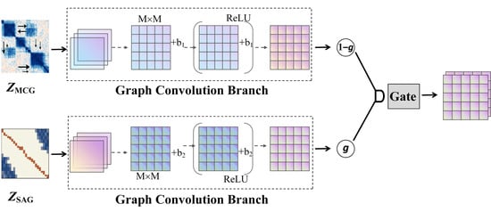
The temporal variance of $\mathrm{g}$ intrinsically quantifies the model’s real-time confidence in the meteorological priors, thereby endowing the architecture with partial physical interpretability. Figure 9 displays the framework of the gated fusion algorithm. When the local atmospheric dynamics exhibit strong physical predictability, the network pushes $\mathit{g}\to 1$, explicitly prioritizing the aerodynamic causal topology and filtering out systematic noise. Conversely, when the physical advection rules fail to explain the power fluctuation, such as sensor anomalies and dispatching interventions, the model adaptively shifts $\mathit{g}\to 0$, redirecting its receptive focus to the data-driven adaptive graph. This design allows the model to flexibly transition between meteorological- and data-dominated spaces without manual intervention.

Figure 9. Framework of the gated fusion mechanism. The gating factor adaptively adjusts the fusion weights of Z_MCG and Z_SAG, enabling the network to dynamically balance the information from multiple sources under varying operational conditions.

3.4. Topology-Aware Selective Scanning Mechanism

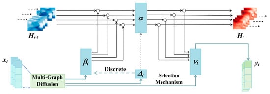
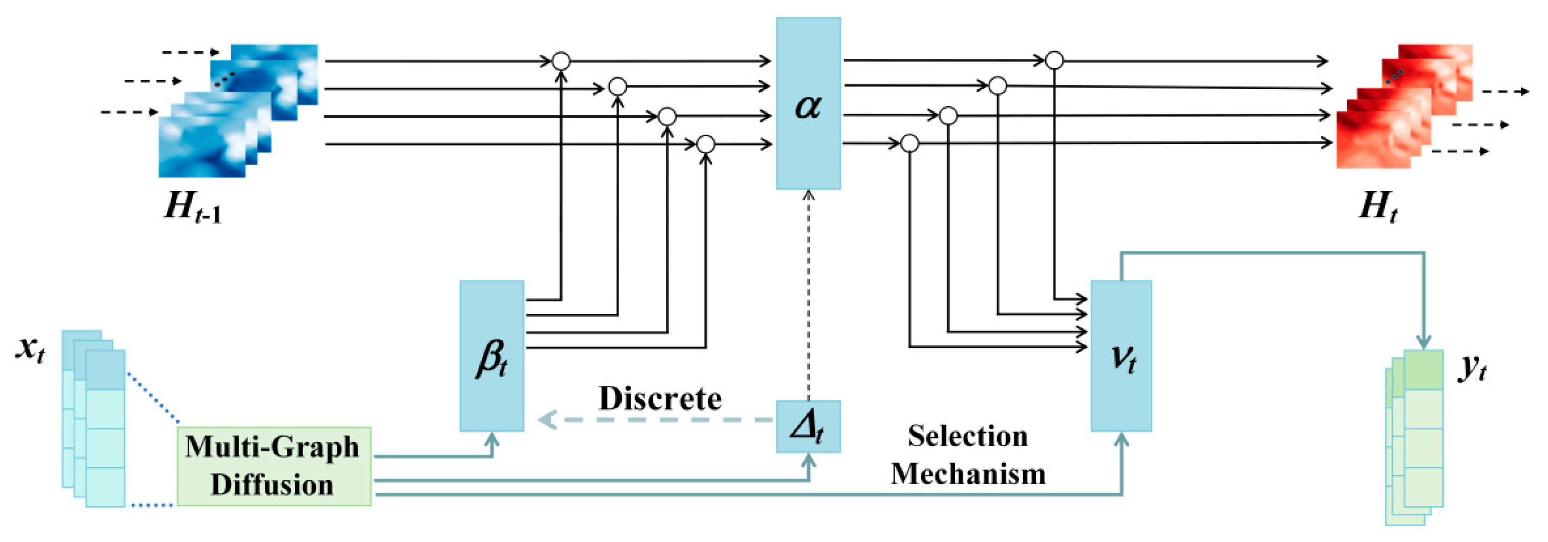
To simultaneously model spatial and temporal dependencies, we adopt a Mamba architecture with multi-graph convolution layers [30]. Mamba is chosen for its efficient long-range sequence modeling and linear-time inference, which complement the local feature extraction capability of convolutions. The framework of Mamba is exhibited in Figure 10, which can be represented in Equations (13) and (14).

$${\mathit{H}}^{\prime }\left(t\right)=\alpha \mathit{H}\left(t\right)+\beta \mathit{X}\left(t\right)$$

(13)

$$\mathit{Y}\left(t\right)=\nu \mathit{H}\left(t\right)$$

(14)

where $\mathit{H}$, $\mathit{Y}$, $\alpha$, $\beta$, and $\nu$ represent the hidden state, output, state transition matrix, input control matrix, and output control matrix, respectively.

Figure 10. The architecture of Mamba. Structured Selective State Space Model independently maps each input channel to output via a high-dimensional latent state.

The state transition matrix defines the system evolution without external input. By compressing historical information into a fixed-dimensional state space, this mechanism enables efficient long-sequence modeling while avoiding the quadratic complexity of attention-based architectures. The matrices $\beta$ and $\nu$ are data-dependent and dynamically generated from the current input. $\mathsf{\alpha }$ is designed as a HiPPO matrix that compresses and stores the historical information, which is provided in Equation (15).

$$\alpha =\left[{\mathsf{\alpha }}_{\mathrm{i}\mathrm{j}}\right]=\left\{\begin{array}{cc}(2i+1{)}^{1/2}(2j+1{)}^{1/2}& i>j\\ i+1& i=j\\ 0& i<j\end{array}\right.$$

(15)

where ${\alpha }_{\mathrm{i}\mathrm{j}}$ denotes the elements of matrix $\mathsf{\alpha }$. We discretize the continuous system using a zero-order hold with a time step of $\mathsf{\Delta }$.

To enable the model to simultaneously capture spatial dependencies during temporal propagation, a topology-aware selective scanning mechanism is designed. Specifically, we replace the original fully connected mappings in Mamba, which are developed for the one-dimensional time series, with graph diffusion convolution operators based on the topology G. To incorporate spatial awareness into the control process, the generation of the time step $\mathsf{\Delta }$ and the control matrices is transformed into a process driven by diffusion convolution operators (Equations (16)–(18)).

$$\Delta \left(t\right)=Softplus\left(W_{\Delta }{\star }_{G}X\left(t\right)+b_{\Delta }\right)$$

(16)

$$\beta \left(t\right)=W_{\beta }{\star }_{G}X\left(t\right)+b_{\beta }$$

(17)

$$\nu \left(t\right)=W_{\nu }{\star }_{G}X\left(t\right)+b_{\nu }$$

(18)

where the diffusion convolution operator of the topology G maps the input signal to the fused graph ${\mathit{Z}}_{\mathrm{h}\mathrm{y}\mathrm{b}\mathrm{r}\mathrm{i}\mathrm{d}}$ in a high-dimensional space.

After discretization, the spatio-temporal state evolution of the Mamba unit can be demonstrated as Equations (19)–(22):

$$\overline{\alpha }\left(t\right)=exp\left(\Delta \left(t\right)\alpha \right)$$

(19)

$$\overline{\beta }\left(t\right)={\left(\Delta \left(t\right)\alpha \right)}^{-1}\left(exp\left(\Delta \left(t\right)\alpha \right)-\mathit{E}\right)\cdot \beta \left(t\right)$$

(20)

$$H\left(t\right)=\overline{\alpha }\left(t\right)H(t-1)+\overline{\beta }\left(t\right){\star }_{G}X\left(t\right)$$

(21)

$$Y\left(t\right)=\nu \left(t\right)H\left(t\right)$$

(22)

where $\mathbf{E}$ is the identity matrix, and $\overline{\mathsf{\alpha }}$ and $\overline{\mathsf{\beta }}$ are the discretized state transition matrix and input control matrix, respectively.

By embedding the diffusion convolution into each time step of the Mamba, the MGDM simultaneously updates the temporal state of each node while aggregating information from its spatially neighboring nodes, achieving joint spatio-temporal dependency modeling and effectively capturing the dynamic coupling relationships among wind turbines.

3.5. Loss Function

To train the MGDM end-to-end, we design a physics-informed joint loss function. The total loss ${\mathcal{L}}_{\mathrm{t}\mathrm{o}\mathrm{t}\mathrm{a}\mathrm{l}}$ is formulated as a weighted combination of three distinct components:

$${\mathcal{L}}_{total}={\mathcal{L}}_{task}+\lambda {\mathcal{L}}_{reg}+\eta \Vert \Theta {\Vert }_2^2$$

(23)

where ${\mathcal{L}}_{\mathrm{t}\mathrm{a}\mathrm{s}\mathrm{k}}$ is the multi-step forecasting task loss, ${\mathcal{L}}_{\mathrm{r}\mathrm{e}\mathrm{g}}$ is the regularization loss, and $\mathsf{\lambda }$ serves as a trade-off coefficient. The final term $\mathsf{\eta }\Vert \mathsf{\Theta }{\Vert }_2^2$ represents the standard ${\mathrm{L}}_2$ weight decay to prevent parametric overfitting, with $\mathsf{\eta }$ being the decay rate.

We employ the Huber Loss [31] as the primary task objective to provide a robust gradient signal across the multi-step horizon ${\mathrm{T}}_1$. The function can be written as Equations (24) and (25).

$$\begin{array}{c}{\mathcal{L}}_{task}={\displaystyle \frac{1}{T_1\times N}}{\sum }_{n=1}^{N}Huber({\widehat{P}}_{t+T_1}^{\left(n\right)},P_{t+T_1}^{\left(n\right)})\end{array}$$

(24)

$$\begin{array}{c}Huber(y,\widehat{y})=\left\{\begin{array}{cc}{\displaystyle \frac{1}{2}}(y-\widehat{y}{)}^2& if|y-\widehat{y}|\le \delta \\ \delta |y-\widehat{y}|-{\displaystyle \frac{1}{2}}{\delta }^2& otherwise\end{array}\right.\end{array}$$

(25)

where $\widehat{\mathrm{P}}$ and $\mathrm{P}$ are the predicted values and ground truth respectively. $\mathsf{\delta }$ is the threshold hyperparameter separating the squared and linear loss regimes.

In terms of regularization loss, the real-time MCG is utilized as a strong structural prior. We penalize the structural divergence between the two topologies using the Frobenius norm, as shown in Equation (26).

$${\mathcal{L}}_{reg}={‖A_{adp}-A_{phy}\left(t\right)‖}_F^2={\sum }_{i=1}^N{\sum }_{j=1}^N{\left(A_{adp}^{(i,j)}-A_{phy}^{(i,j)}(t)\right)}^2$$

(26)

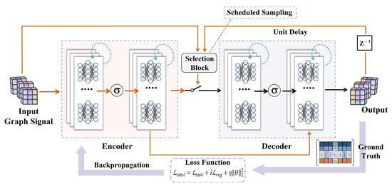
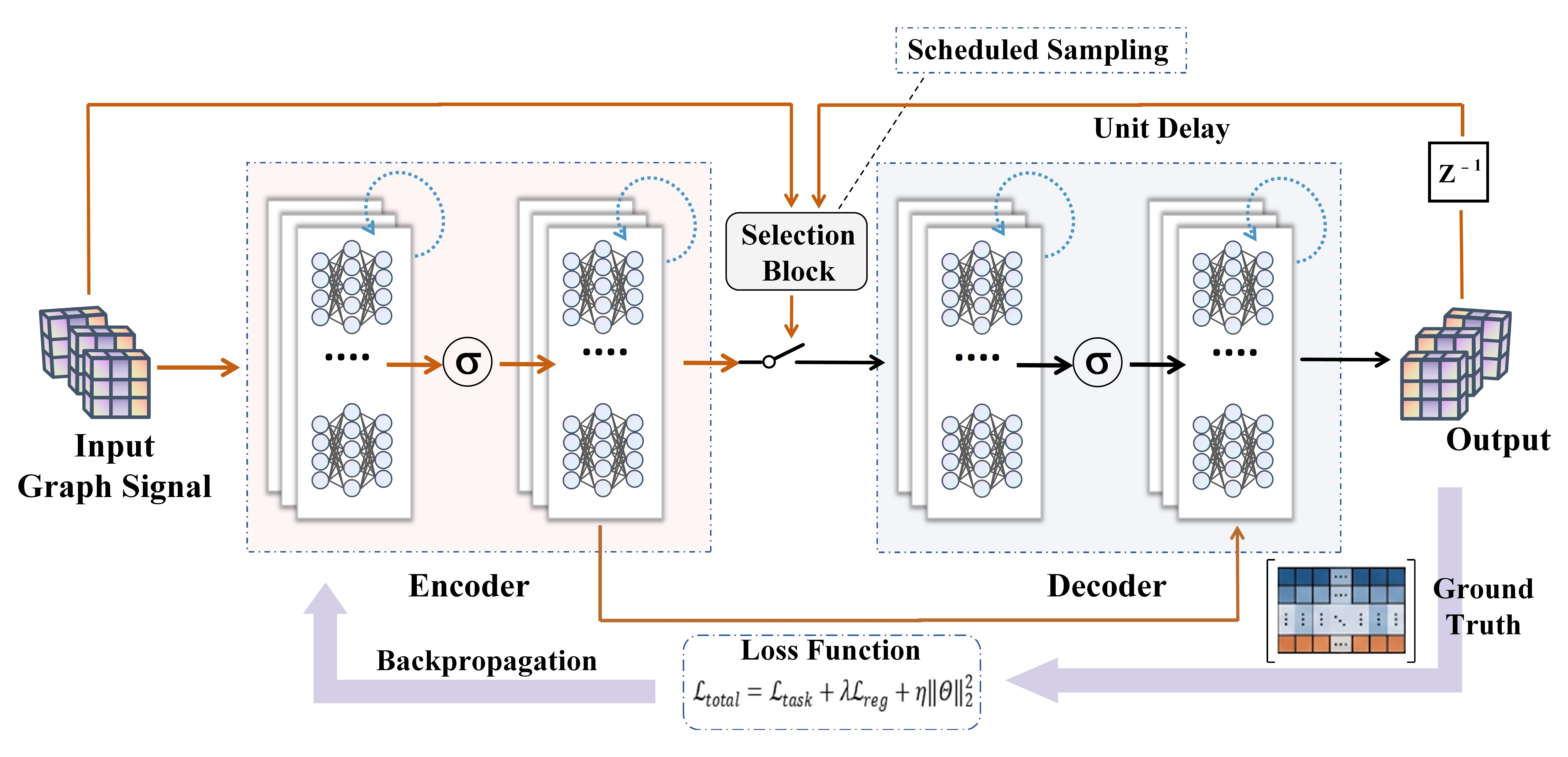
The model is optimized by the AdamW optimizer using the Backpropagation Through Time (BPTT) algorithm. We adopt a Seq2Seq architecture with the MGDM-based encoder and decoder [29], as depicted in Figure 11.

Figure 11. End-to-end framework of the Multi-Graph Diffusion Mamba for wind power forecasting. Historical data are fed into an encoder module to capture latent spatio-temporal representations. The encoded features are delivered to the subsequent decoder module. During training, the decoder receives input alternately from ground-truth signals and prior model estimations controlled by the scheduled sampling selection block.

The model is evaluated in a strictly autonomous closed-loop recursive method: scheduled sampling is used only during training to mitigate exposure bias [32,33,34] and disabled at test time. The ground truth of the future power is used solely for training loss and test metrics, never as decoder input at any forecasting step.

Specifically, for an arbitrary test sequence targeting a forecast horizon of T steps ahead ($k\in \{1,\dots ,T\}$) initialized at forecast point t, the step-by-step inference pipeline proceeds as follows:

(1) Historical State Encoding: The encoder receives the standardized historical sequence $P_{(t-T+1):t}$ and meteorological features $F_{(t-T+1):t}$ across the look-back window T. The temporal hidden states and dual-graph spatial dependencies are jointly updated, and the terminal hidden state $H_{enc}\left(t\right)$ is utilized to initialize the recurrent hidden state of the decoder $H_{dec}\left(0\right)$.

(2) Single-step Ahead Prediction: For the initial forecasting step, the decoder input consists of the last available historical observation at the forecast point t, denoted as ($P_t,F_t$). Note that $P_t$ is the last observed power value at the forecast point and is legitimately available at prediction time. The network executes graph diffusion and selective state scanning to output the first-step power ${\widehat{P}}_{t+1}$.

(3) Closed-loop Autoregressive Rollout: For all subsequent forecasting horizons, the input power variable to the decoder is strictly and recursively substituted by the model’s own prior prediction ${\widehat{P}}_{t+k-1}$. The input vector at step k is formulated as (${\widehat{P}}_{t+k-1}$,${\widehat{F}}_{t+k-1}$), where ${\widehat{F}}_{t+k-1}$ denotes the meteorological feature vector available at forecasting step k.

(4) Continuous State Updates and Multi-step Output: The hidden state evolves recursively as $H_{dec}(k)=MGDM[H_{dec}(k-1),({\widehat{P}}_{t+k-1},{\widehat{F}}_{t+k-1})]$ without any external ground-truth feedback, generating the multi-step trajectory $\left\{{\widehat{P}}_{t+1},{\widehat{P}}_{t+2},\dots ,{\widehat{P}}_{t+T}\right\}$.

In this study, to ensure an unbiased and realistic performance comparison, all the baselines are evaluated under the identical closed-loop recursive rollout constraints.

4. Case Study

This section presents an experimental evaluation of the proposed MGDM framework. First, comparative tests with five baselines show that MGDM consistently achieves lowest error metrics (in terms of NRMSE and NMAE) alongside the highest determination coefficients (R²) across all turbines and forecasting horizons. Second, ablation studies confirm the indispensability of EWT preprocessing, the dual-graph topology, and the Mamba module; removing any component causes notable error growth, with RNN replacement leading to the most severe degradation. Third, gating observations reveal that the gating factor adaptively balances physical and data-driven branches, dropping under extreme conditions to avoid invalid predictions. Finally, sensitivity analysis identifies $\mathsf{\lambda }\approx 0.352$ as the optimal trade-off between physical constraints and data flexibility.

4.1. Experimental Configuration

The hyperparameter configuration of the proposed framework in this study is summarized in Table 2. All experiments are implemented using Python 3.10 and PyTorch 2.30 on a Windows 11 workstation equipped with a 13th Gen Intel i7-13700H processor (2.40 GHz) and an NVIDIA RTX 3050 GPU.

Table 2. Hyperparameter configurations of the proposed paradigm.

Hyperparameter	Notation	Value
Look-Back Window	T0	24
Forecasting Horizon	T1	{1,4,8,12,16}
EWT Modes	-	4
Number of Nodes	N	4
Diffusion Steps	K	2
TE Binning Partition	B	13
Wind Direction Sectors	S	8
Latent Embedding Dim	de	8
Core Hidden Dimension	dmodel	64
SSM State Dimension	dstate	16
Huber Threshold	δ	1
Trade-off Weight	λ	0.35
L2 Regularization	η	10−4
Initial Learning Rate	lr	10−3
Batch Size	-	64
Early Stopping Patience	-	15

To assess the predictive capability of the proposed model, three metrics are adopted in this study: Mean Absolute Error (MAE), Root Mean Squared Error (RMSE), and the Coefficient of Determination (R²). All error metrics are computed based on both normalized power values and their corresponding original physical units, ensuring that the evaluation results are both physically interpretable and comparable across different models [35]. The corresponding formulations are provided in Equations (27)–(29).

$$NMAE={\displaystyle \frac{1}{n}}{\sum }_{i=1}^n{\displaystyle \frac{\left|P_i-{\widehat{P}}_i\right|}{P_{rated}}}$$

(27)

$$NRMSE=\sqrt{{\displaystyle \frac{1}{n}}{\sum }_{i=1}^n{\left({\displaystyle \frac{P_i-{\widehat{P}}_i}{P_{rated}}}\right)}^2}$$

(28)

$$R^2=1-{\displaystyle \frac{{\sum }_{i=1}^n{\left(P_i-{\widehat{P}}_i\right)}^2}{{\sum }_{i=1}^n{\left(P_i-E\left(P\right)\right)}^2}}$$

(29)

where $\mathrm{n}$ is the sample size, ${\mathrm{P}}_{\mathrm{i}}$ and ${\widehat{\mathrm{P}}}_{\mathrm{i}}$ are the predicted and actual power values at time step $\mathrm{i}$, respectively, ${\mathrm{P}}_{\mathrm{r}\mathrm{a}\mathrm{t}\mathrm{e}\mathrm{d}}$ is the rated power capacity, and $\mathrm{E}\left(\mathrm{P}\right)$ denotes the expected value of the power.

To guarantee experimental rigor, all the models were supplied with identical multivariate input channels across the identical historical look-back window, adhering to uniform chronological partitioning and training-derived Min-Max normalization. Hyperparameters for each model were systematically navigated via grid search on the validation partition using identical early-stopping patience (15 epochs). To account for stochastic weight initialization and training variability, all experiments were repeated across five independent runs with distinct random seeds; the performance metrics reported in Table 3 represent the mean values across these repeated runs (with standard deviations consistently below 0.0018 in NRMSE).

Table 3. Multi-step wind power forecasting performance across five horizons for FD1.

Model	Time Steps	NRMSE	NMAE
MGDM	1 (15 min)	0.0253	0.0183
	4 (1 h)	0.0437	0.0303
	8 (2 h)	0.0913	0.0600
	12 (3 h)	0.1333	0.1079
	16 (4 h)	0.1527	0.1213
GWNet	1 (15 min)	0.0591	0.0426
	4 (1 h)	0.0713	0.0472
	8 (2 h)	0.1395	0.0944
	12 (3 h)	0.1685	0.1259
	16 (4 h)	0.1916	0.1417
ASTGCN	1 (15 min)	0.0622	0.0507
	4 (1 h)	0.1066	0.0745
	8 (2 h)	0.1724	0.1450
	12 (3 h)	0.2049	0.1512
	16 (4 h)	0.2262	0.1947
STGCN	1 (15 min)	0.0481	0.0358
	4 (1 h)	0.0901	0.0731
	8 (2 h)	0.1313	0.1010
	12 (3 h)	0.1611	0.1199
	16 (4 h)	0.1891	0.1586
TCN	1 (15 min)	0.1083	0.0857
	4 (1 h)	0.1722	0.1283
	8 (2 h)	0.1960	0.1329
	12 (3 h)	0.2407	0.1831
	16 (4 h)	0.2629	0.2091
FC-LSTM	1 (15 min)	0.0936	0.0718
	4 (1 h)	0.1846	0.1455
	8 (2 h)	0.1927	0.1495
	12 (3 h)	0.2383	0.1702
	16 (4 h)	0.2680	0.2128

4.2. Comparative Evaluation of Forecasting Performance

To evaluate the forecasting performance of the proposed MGDM framework, five typical benchmark models are selected for comparison: TCN, FC-LSTM, STGCN, ASTGCN, and GWNet. These models represent different paradigms, including pure temporal methods, static spatio-temporal graph networks, and data-driven adaptive graph architectures. To guarantee an unbiased and rigorous comparison, the proposed model and the five benchmark architectures were evaluated under strictly standardized experimental conditions, including identical input features and splitting, standardized hyperparameter tuning, and a uniform training environment. All models are tested across five multi-step forecasting horizons ranging from one step (15 min) to 16 steps (4 h). Table 3 demonstrates the forecasting results for turbine FD1 across five horizons. At the 1-step horizon, all models achieve R² above 0.80. As the horizon extends to 16 steps, purely temporal models (TCN and FC-LSTM) suffer from severe error accumulation and NRMSE growth due to the lack of spatial constraints. Graph-based models (STGCN, ASTGCN) can improve short-term performance via spatial convolution but remain constrained by fixed topologies derived from geographical proximity or symmetric statistics, which fail to capture directional, time-varying wind propagation. Among all baselines, GWNet demonstrates the most robust comprehensive capability when evaluated across all four turbines on average and maintains superior long-horizon determination coefficients (R² = 0.747 at 16 steps), benefiting from its learnable adaptive adjacency matrix. However, its purely data-driven nature makes it susceptible to overfitting noise and local fluctuations.

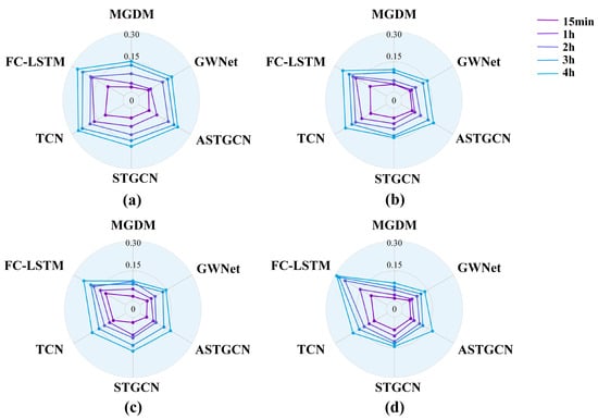
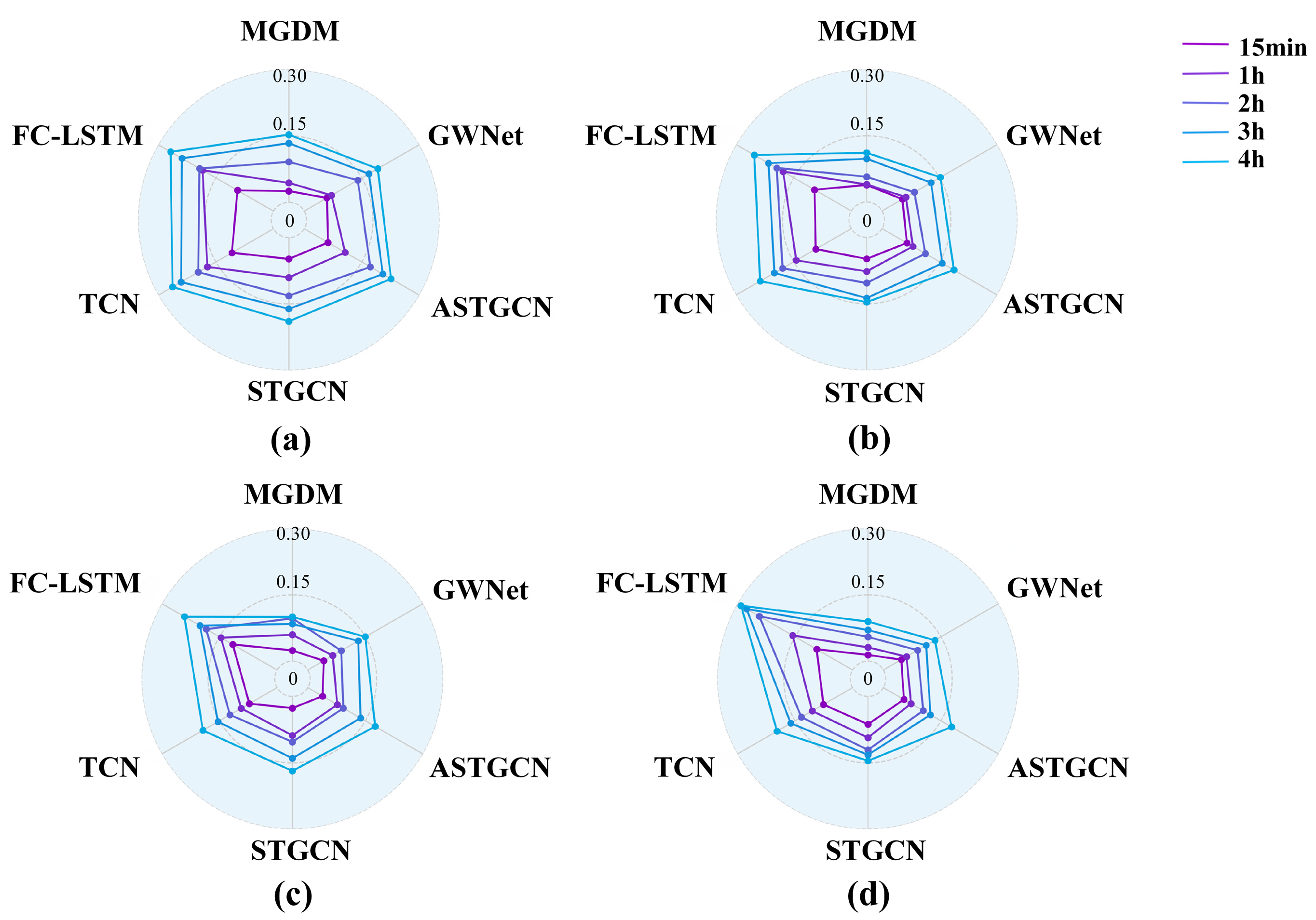
The proposed MGDM consistently outperforms all baselines across five horizons, achieving a NRMSE of 0.0253 at 15 min and 0.1527 at 4 h, with an R² of 0.941 and 0.773, respectively. This superior performance confirms the synergistic benefits of our design: the multi-graph fusion decouples physical wake propagation from latent operational constraints, while the topology-aware Mamba module mitigates long-sequence memory decay. Figure 12 presents the radar charts of NRMSE distribution across all turbines, where the MGDM consistently occupies the innermost vertex on each axis, confirming its robust and stable performance.

Figure 12. Radar charts of the multi-horizon NRMSE variations across four wind turbines. (a) FD1, (b) FD2, (c) FD3, (d) FD4.

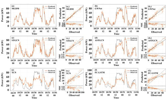
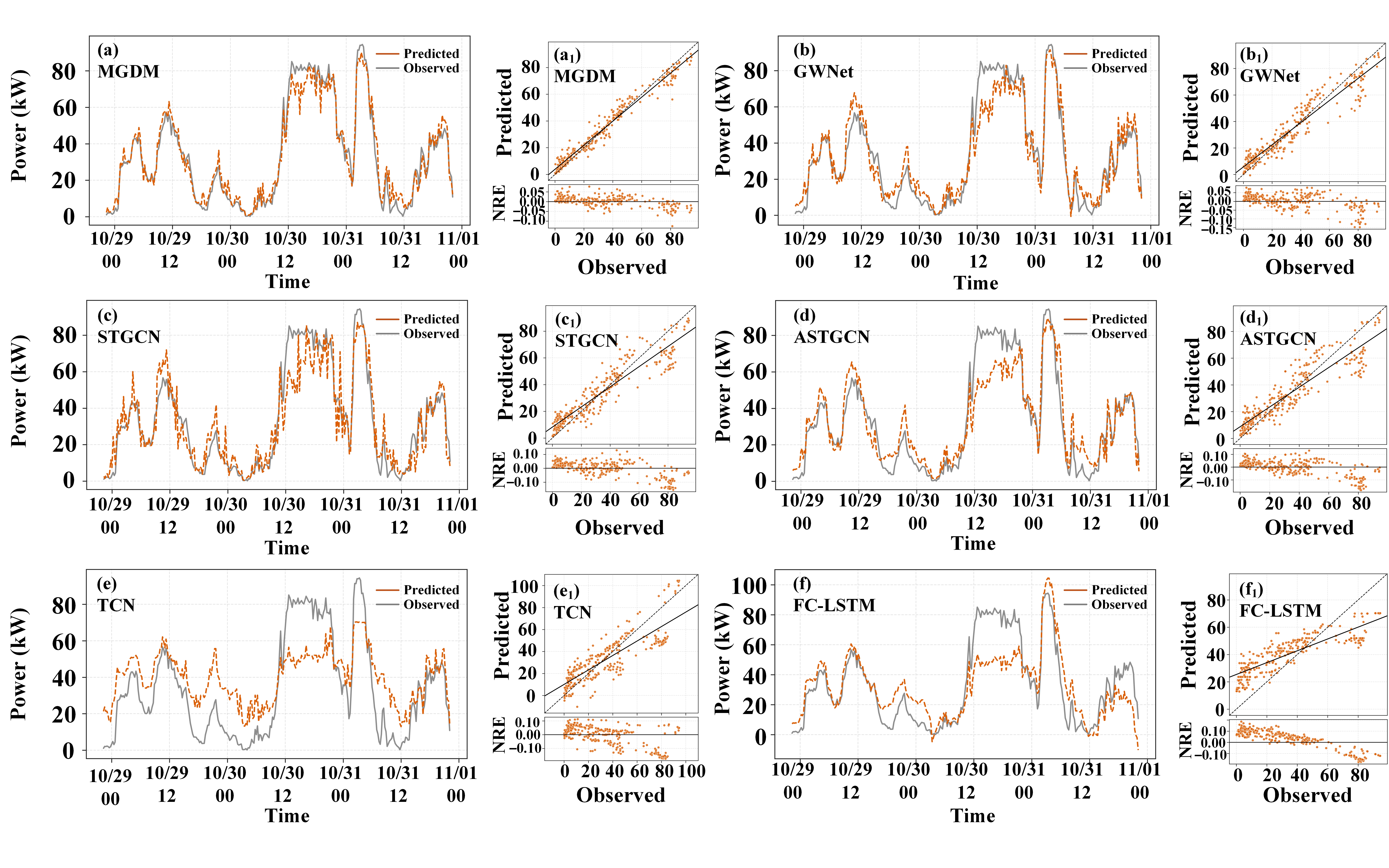
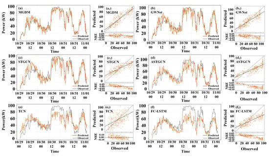
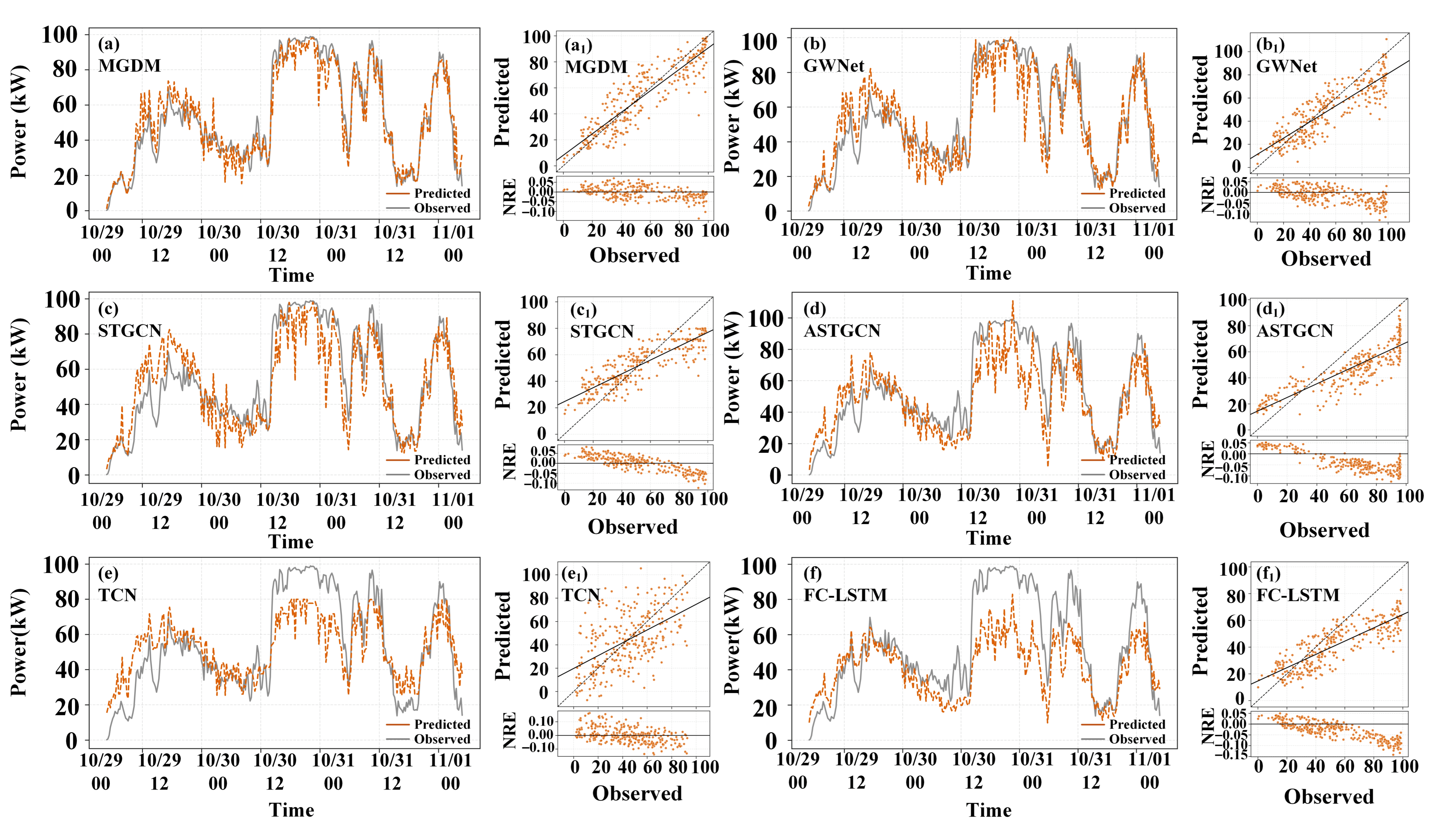
Figure 13 and Figure 14 present the 1 ha head forecasting trajectories for turbines FD1 and FD2 over a three-day period in late October, 2019. The line charts show that most baseline algorithms struggle with sharp power fluctuations. TCN and FC-LSTM exhibit pronounced phase lags and frequently fail to capture peak or valley generation states. ASTGCN and STGCN, constrained by fixed graph structures, display significant overshoots and undershoots in response to abrupt wind regime changes. GWNet occasionally misses sudden rise events by its purely data-driven topology, which tends to misinterpret transient aerodynamic stalls or curtailments as noise. In contrast, MGDM more closely follows the ground-truth trajectory, demonstrating improved sensitivity to high-frequency transients and extreme turning points. What is more, the scatter plots and residual error distributions show that the predictions of the MGDM cluster more densely and symmetrically along the ideal diagonal line, with residuals narrowly distributed around zero.

Figure 13. Time series and scatter plots comparing the predicted with the observed wind power across different models in FD1. The subplots are categorized into the proposed MGDM model (a,a₁), the adaptive paradigm (GWNet) (b,b₁), conventional spatio-temporal networks (STGCN, ASTGCN) (c,d,c₁,d₁), and pure temporal benchmarks (TCN, FC-LSTM) (e,f,e₁,f₁). The forecast horizon is 1 h (4 time steps) during a three-day period in late October, 2019. The lower panels in the scatter charts represent the corresponding continuous Normalized Residual Error (NRE) distributions.

Figure 14. Time series and scatter plots comparing the predicted with the observed wind power across different models in FD2. The subplots are categorized into the proposed MGDM model (a,a₁), the adaptive paradigm (GWNet) (b,b₁), conventional spatio-temporal networks (STGCN, ASTGCN) (c,d,c₁,d₁), and pure temporal benchmarks (TCN, FC-LSTM) (e,f,e₁,f₁). The forecast horizon is 1 h (4 time steps) during a three-day period in late October, 2019. The lower panels in the scatter charts represent the corresponding continuous Normalized Residual Error (NRE) distributions.

As shown in Table 4, the MGDM contains approximately 0.70 M parameters, comparable to lightweight baselines yet substantially fewer than heavier models such as ASTGCN. Its FLOPs are approximately 0.38 M, significantly lower than these ®®petitive models. Given its superior performance across all forecasting horizons, this computational overhead remains within practically acceptable limits. Moreover, the linear scanning mechanism avoids quadratic complexity and supports parallel computation during training, making it suitable for real-time deployment.

Table 4. Comparison of model computational complexity and theoretical scaling under standardized configurations.

Model	Backbone Architecture	Params	FLOPs	Complexity Scaling (Time)
MGDM	Multi-graph Diffusion + Mamba	≈0.70 M	≈0.38 M	O (K + T0) (Parallel Scan)
GWNet	Adaptive Graph + TCN	≈0.85 M	≈0.55 M	O (T) (Parallel)
ASTGCN	Spatial & Temporal Attention	≈1.75 M	≈2.10 M	O (T2) (Attention)
STGCN	Spectral Graph + 1D Conv	≈0.42 M	≈0.22 M	O (T) (Parallel)
TCN	Dilated 1D Conv	≈0.30 M	≈0.18 M	O (T) (Parallel)
FC-LSTM	RNN	≈0.25 M	≈0.15 M	O (T) (Sequential)

Note. FLOPs and parameter counts were benchmarked using the standard thop profiling toolkit based on an input tensor batch of shape, adhering to the multiply–accumulate counting standard (1 MAC = 2FLOPS).

4.3. Ablation Studies

To gain insight into the contribution of each component, an ablation analysis is conducted. All metrics are computed exclusively on the test set. The proposed model is systematically ablated into five groups:

Group 1 (full model): The MGDM.

Group 2 (w/o EWT): Removes the EWT preprocessing. Raw, non-stationary meteorological and power sequences are fed directly into the network.

Group 3 (w/o MCG): Removes the branch of MCG. The spatial diffusion relies solely on the data-driven SAG, degrading to an undirected graph convolution process.

Group 4 (w/o SAG): Removes the SAG and its learnable node embeddings. Spatial aggregation is strictly constrained by the MCG.

Group 5 (w/o Mamba): Replaces the Mamba with a Recurrent Neural Network (RNN).

As presented in Table 5, the contribution of each core component is quantified. Removing EWT (G2) causes a modest accuracy drop (e.g., FD3 NRMSE from 0.0241 to 0.0317), confirming its effectiveness in suppressing high-frequency noise. The multi-graph topology proves indispensable: ablating the physical branch (G3) raises FD1 NRMSE from 0.0253 to 0.0631, while removing the adaptive branch (G4) leads to even larger errors on downstream turbine FD2, indicating that neither physical priors nor data-driven learning alone suffices. Replacing Mamba with a standard RNN (G5) causes the most severe degradation (e.g., NRMSE = 0.1124 in FD3), confirming that the selective scan mechanism effectively prevents long-term memory decay and ensures robust spatio-temporal modeling.

Table 5. Ablation study of the MGDM on the test set across four turbines.

Group	EWT	MCG	SAG	Temporal Architecture	NRMSE
					FD1	FD2	FD3	FD4
G1	✓	✓	✓	Mamba	0.0253	0.0386	0.0241	0.0141
G2		✓	✓	Mamba	0.0278	0.0401	0.0317	0.0182
G3	✓		✓	Mamba	0.0631	0.0853	0.0628	0.0706
G4	✓	✓		Mamba	0.0722	0.0967	0.0593	0.0814
G5	✓	✓	✓	RNN	0.0762	0.1071	0.1124	0.0896

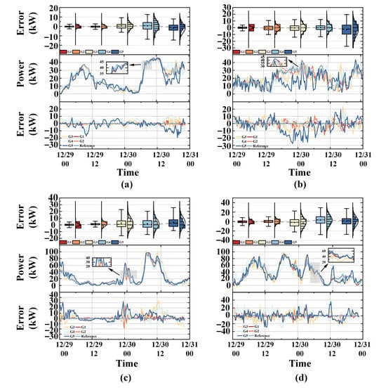
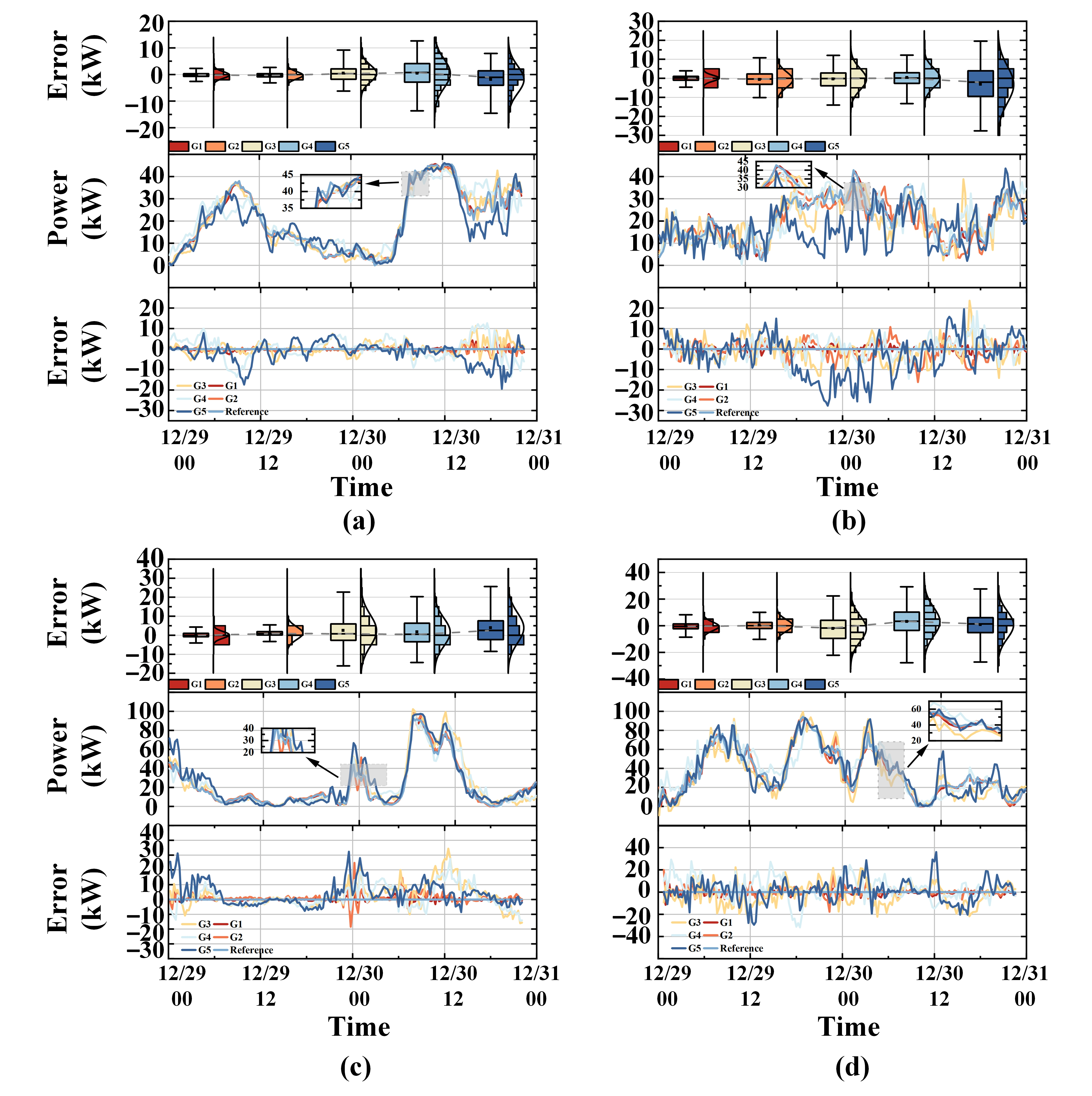
Figure 15 compares the prediction errors and tracking performance of the five variants during a volatile 48 h winter period. The full model (G1) consistently yields the smallest, most concentrated errors and tracks the true power trajectories with the most symmetric residuals, confirming its superior accuracy and robustness. By contrast, G2–G4 exhibit asymmetric error distributions and pronounced outliers, with G3 and G4 showing persistent tracking hysteresis during sudden power ramps, indicating that removing either EWT or the causal graph branch compromises non-stationary handling. G5 shows the largest error inflation and produces high-amplitude residual spikes under transient shocks, highlighting the critical role of the selective scan mechanism in long-range temporal modeling.

Figure 15. Ablation study results over a 48 h volatile winter period (29–31 December 2019). The full model (G1) yields the smallest and most concentrated errors, while G2–G4 show asymmetric distributions and outliers, and G5 exhibits the largest error inflation—confirming the critical roles of the multi-graph topology and the selective scan mechanism. Panels (a–d) correspond to turbines FD1–FD4, respectively.

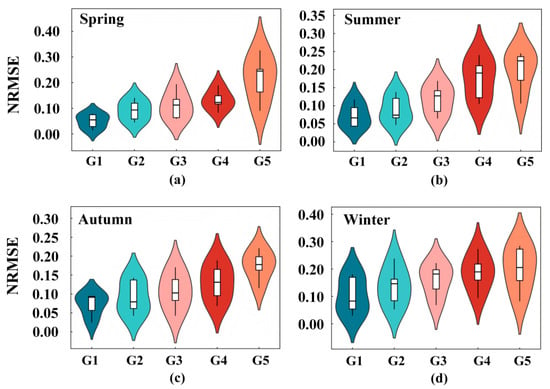
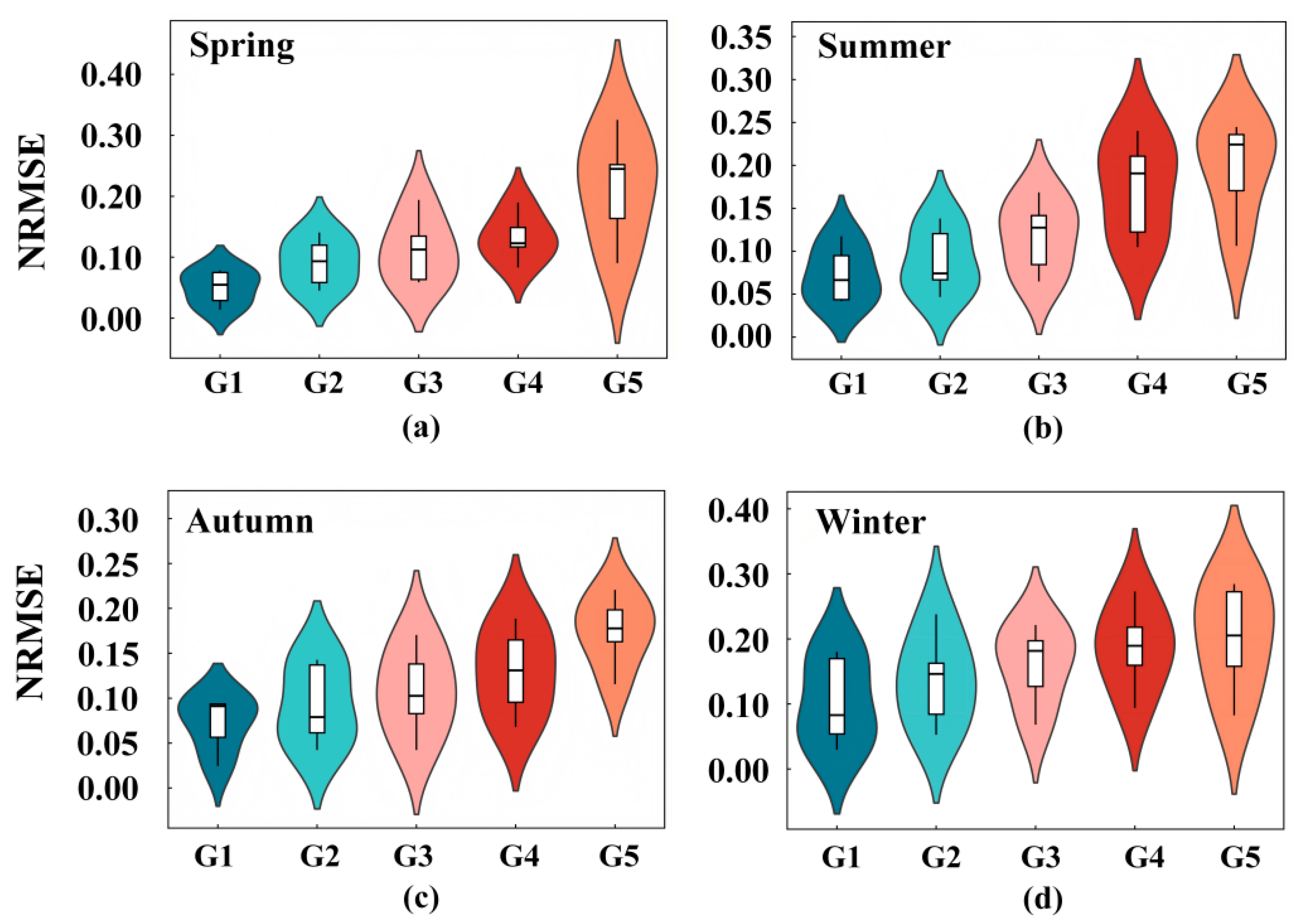
Figure 16 compares the seasonal error distributions across five horizons (one to 16 steps) for turbine FD1. The full model (G1) consistently achieves the lowest median errors throughout the year, confirming the robustness of the multi-graph diffusion and selective scan mechanism under diverse meteorological conditions. In contrast, G5 exhibits the largest spread and highest medians, particularly in winter, where errors reach 0.40, highlighting the memory decay of RNN-based structures under seasonal shifts. Removing EWT (G2) or spatial routing branches (G3, G4) also widens the interquartile range (IQR) and produces asymmetric upper tails, though to a lesser extent than G5.

Figure 16. Seasonal multi-horizon error distribution for FD1 across (a) Spring, (b) Summer, (c) Autumn, and (d) Winter.

4.4. Interpretability of the Dynamic Gating Mechanism

To investigate the internal mechanism of the proposed multi-graph fusion architecture, we investigate the variation in the dynamic gating factor $g$ under two specific scenarios: (1) extreme weather conditions (gale-force winds); and (2) grid dispatch (power curtailment). Taking FD1 as an example, the gating factor serves as an adaptive controller, dynamically balancing the information from the physics-based meteorological priors and the data-driven systemic residuals.

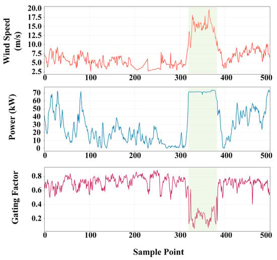
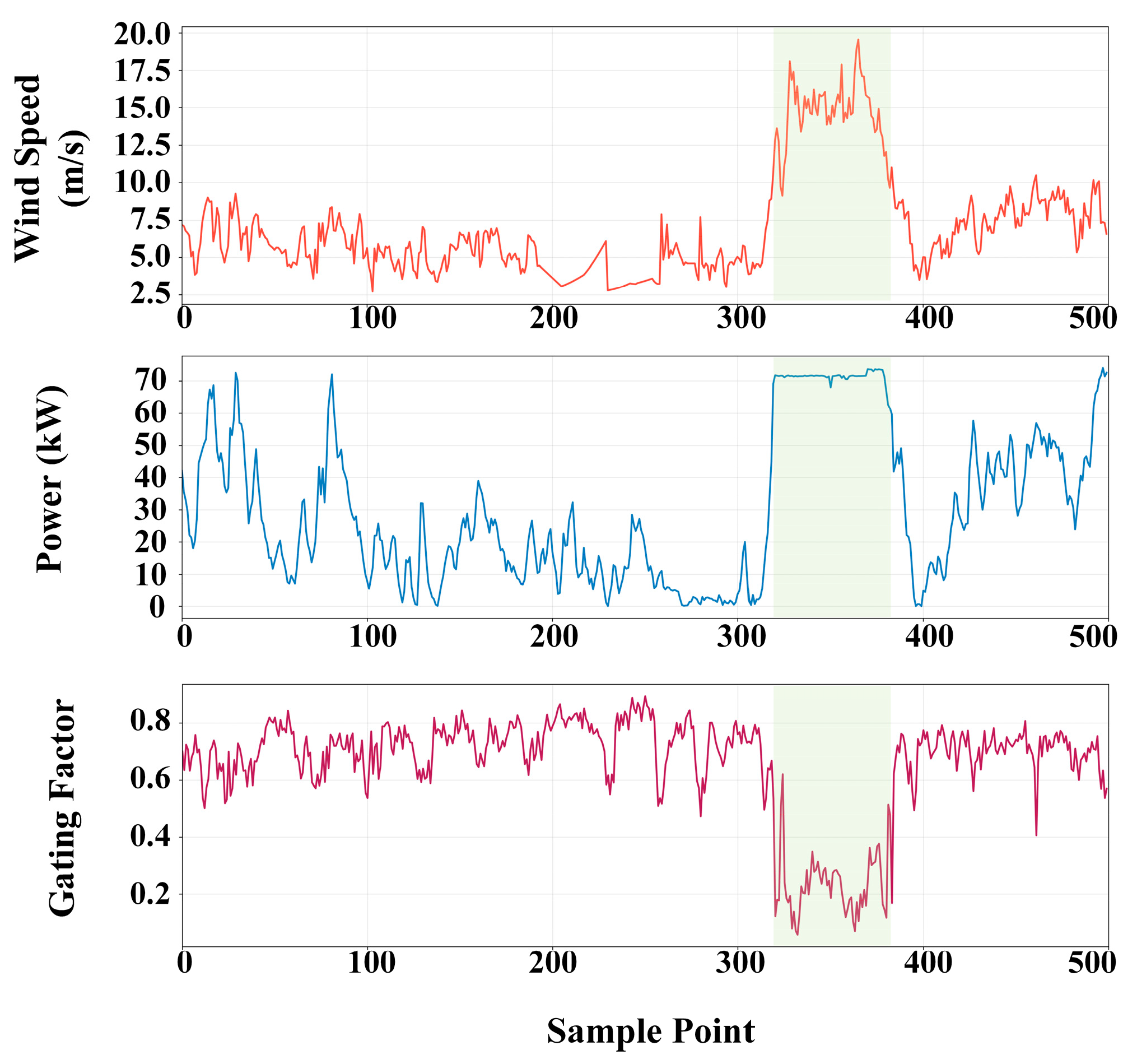
As depicted in Figure 17, under standard operational conditions, $g$ remains consistently elevated within a narrow band between 0.6 and 0.8, indicating that the network predominantly relies on the meteorological condition as the primary driver. However, during the extreme weather event when the wind speed abruptly exceeds 15 m/s, the turbine activates pitch control, making the power output saturate. The physical saturation was captured by the model, causing a prominent drop in the gating factor. This adaptive fusion mechanism can prevent the network from erroneously predicting unrealistic power outputs under saturation events.

Figure 17. Dynamic response of the gating factor $\mathrm{g}$ to extreme weather conditions (gale-force winds). Shaded intervals indicate active pitch control regimes under extreme conditions.

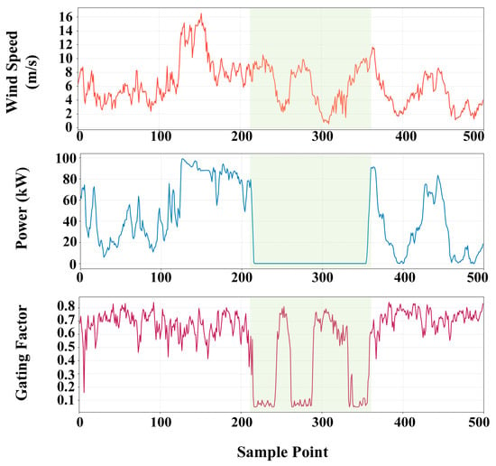
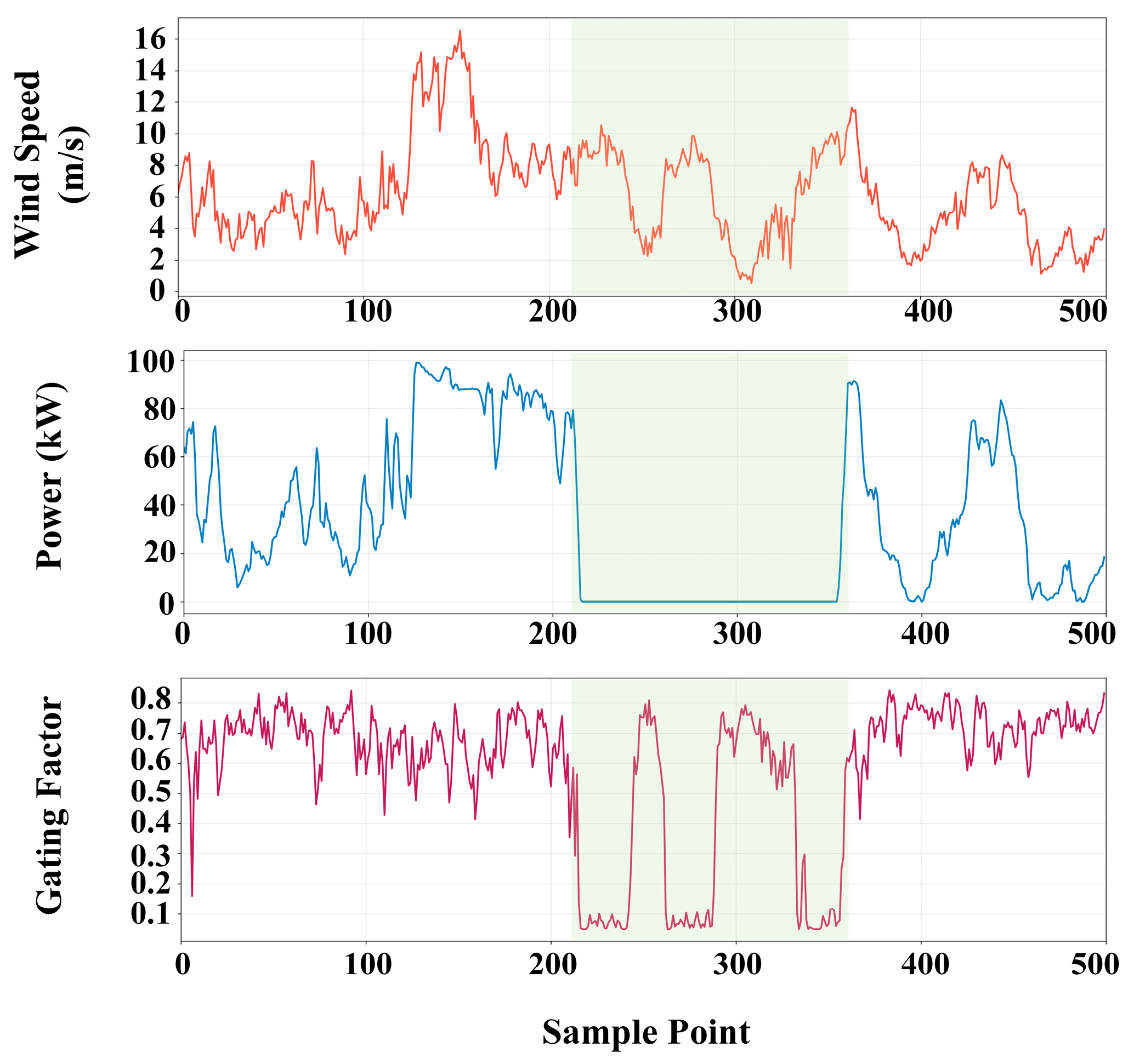
Figure 18 presents a case of active power curtailment by grid operator. During this period, wind speeds remain favorable, fluctuating between 2 m/s and 12 m/s, but the actual power output is capped at nearly 0 kW due to external dispatch commands. In response, $g$ has been driven down frequently by the dynamic gating mechanism, and the model effectively maintains the prediction accuracy.

Figure 18. Dynamic response of the gating factor $\mathrm{g}$ to grid dispatch (power curtailment). Shaded intervals denote grid curtailment periods where active power is artificially constrained despite favorable wind speeds.

The results indicate that the dynamic gating factor $\mathrm{g}$ serves as an interpretable adaptive mechanism. Although operational SCADA records lack direct blade strain gauges and turbine micrositing coordinates remain confidential, the observed variations in $g$ exhibit strong behavioral alignment with known aerodynamic and operational regimes. By adjusting its value in response to the changing conditions, the model can flexibly transition between meteorological-dominated and data-dominated regimes without manual intervention.

4.5. Sensitivity Analysis of Hyperparameter $\lambda$

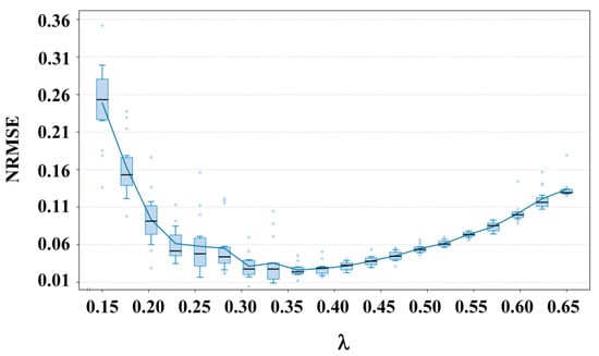
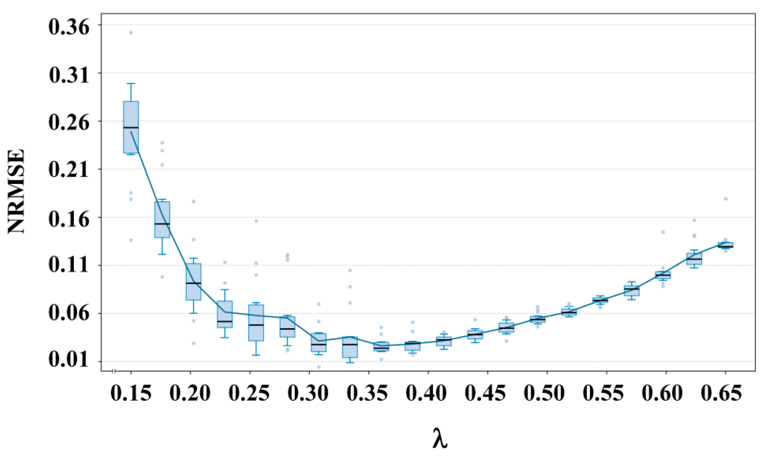
To investigate the impact of the trade-off weight on forecasting performance, we conduct a sensitivity analysis on $\lambda$, which balances the physical meteorological priors and data-driven residuals during joint optimization. For turbine FD1, Figure 19 shows the NRMSE distribution as $\lambda$ varies from 0.15 to 0.65. Centerlines indicate the median; lower and upper box edges represent the 25th and 75th percentiles (interquartile range, IQR); and whiskers extend to 1.5 × IQR; points denote statistical outliers.

Figure 19. Sensitivity analysis of the trade-off weight $\mathsf{\lambda }$. The NRMSE distribution is shown as $\mathsf{\lambda }$ varies from 0.15 to 0.65. The optimal value is approximately 0.352: smaller $\mathsf{\lambda }$ causes overfitting to noise (median NRMSE > 0.20, widened IQRs), while larger $\mathsf{\lambda }$ over-constrains the model and degrades accuracy.

In the under-constrained region ($\lambda <0.3$), physical constraints are too weak to penalize deviations from meteorological priors. As a result, the model overfits localized noise, leading to substantial performance degradation: the median NRMSE exceeds 0.20 and the IQRs widen markedly.

As $\lambda$ approaches 0.35, the NRMSE reaches its minimum, with the narrowest IQR and fewest outliers. The sensitivity analysis reveals that $\lambda \approx 0.352$ strikes an optimal balance between physical constraint enforcement and adaptive flexibility for unobserved conditions.

As $\lambda$ increases beyond 0.40, the NRMSE rises monotonically. Although the variance remains relatively narrower than in the under-constrained regime, the absolute predictive accuracy systematically degrades. and the model becomes overly anchored to deterministic physical wind flows, limiting the adaptive branch’s ability to adjust the graph topology when grid dispatching contradicts the natural aerodynamic potential.

5. Conclusions

This study proposes an innovative Multi-Graph Diffusion Mamba (MGDM) framework for ultra-short-term wind power forecasting, aiming to achieve the dynamic integration of meteorological mechanisms with adaptive data-driven approaches, and the synergistic modeling of spatio-temporal relationships. The multi-graph architecture decouples dependencies among turbines into a physics-informed Meteorological Causal Graph (MCG) and a data-driven Systemic Adaptive Graph (SAG), while a dynamic gated fusion mechanism adaptively balances the two branches through a real-time confidence factor. Additionally, a topology-aware selective scanning module embedding graph diffusion into the Mamba backbone is introduced to achieve joint spatio-temporal modeling.

Experimental results demonstrate that the MGDM consistently outperforms the mainstream baselines across all forecasting horizons. Ablation studies further confirm that both the multi-graph topology and the selective scan mechanism are indispensable for robust performance under non-stationary conditions. Moreover, the gating factor is explored to serve as an interpretable indicator of regime switching, reflecting the proposed mechanism of adaptive balance between the two branches under varying conditions. Sensitivity analysis on the trade-off weight $\mathsf{\lambda }$ identifies $\mathsf{\lambda }\approx 0.352$ as the optimal setting, balancing physical constraints and data flexibility.

We would like to point out that the proposed framework are validated on a single wind farm, lacking verification on large-scale wind farm clusters with more complex wake interactions. Additionally, while this study benchmarks MGDM against an extensive spectrum of deep learning and graph architectures, standard naive persistence models were not formally included in the comparative evaluation. Moreover, the performance under more extreme meteorological scenarios, such as typhoons and icing disasters, has not been exhaustively explored. Future work will be done to extend the framework to diverse wind farms, develop specialized modules for extreme-condition forecasting, and adapt the model to multiple temporal resolutions and longer prediction lengths to meet various dispatch needs.

References

- Li, C.; Xu, Y.; Sun, H. An end-to-end cost-focused wind power forecasting framework based on convex hulls. IEEE Trans. Power Syst. 2026, 41, 2414–2417. [Google Scholar] [CrossRef] [Scilit]
- Wan, C.; Luo, Y.; Wu, W.; Hatziargyriou, N.D.; Lei, S. Day-ahead wind power ramp events prediction with extreme-value-driven learning and confidence-aware detection. IEEE Trans. Sustain. Energy 2026, 17, 3296–3308. [Google Scholar] [CrossRef] [Scilit]
- Gijón, A.; Eiraudo, S.; Manjavacas, A.; Bottaccioli, L.; Lanzini, A.; Molina-Solana, M.; Gómez-Romero, J. Explainable hybrid semi-parametric model for prediction of power generated by wind turbines. In Computational Science—ICCS 2024; Springer Nature: Cham, Switzerland, 2024; pp. 299–306. [Google Scholar]
- Wang, X.; Zhou, Y. Privacy-preserving probabilistic wind power forecasting: An adaptive federated approach. Appl. Energy 2025, 396, 126177. [Google Scholar] [CrossRef] [Scilit]
- Meng, Z.; Guo, Y.; Zhao, C. Probabilistic wind power forecasting with missing data tolerance: An end-to-end nonparametric approach. IEEE Trans. Sustain. Energy 2026, 17, 1202–1213. [Google Scholar] [CrossRef] [Scilit]
- Wang, Y.; Xu, H.; Huang, Y.; Zhang, F.; Kou, H.; Zou, R.; Hu, Q.; Srinivasan, D. An end-to-end ensemble learning approach for enhancing wind power forecasting. IEEE Trans. Sustain. Energy 2026, 17, 435–448. [Google Scholar] [CrossRef] [Scilit]
- Yang, M.; Xu, C.; Bai, Y.; Ma, M.; Su, X. Investigating black-box model for wind power forecasting using local interpretable model-agnostic explanations algorithm. CSEE J. Power Energy Syst. 2025, 11, 227–242. [Google Scholar] [CrossRef] [Scilit]
- Dong, X.; Sun, Y.; Zhang, X.; Mei, S. Wind power forecasting based on multi-task learning with shared latent space mapping. CSEE J. Power Energy Syst. 2025, 1–10. [Google Scholar]
- Xu, C.; Cui, S.; Wei, L.; Zhu, B.; Ai, X.; Fang, J.; Wen, J. Wind power forecasting under extreme weather: A novel few-shot learning architecture. IEEE Trans. Sustain. Energy 2026, 17, 788–803. [Google Scholar] [CrossRef] [Scilit]
- Wu, Z.; Shi, Y.; Gu, T.; Xia, M. VSTCformer for Wind Power Interval Forecasting via Adaptive Variational Mode Decomposition and Spatio-Temporal Cross-Attention. Appl. Sci. 2026, 16, 7470. [Google Scholar] [CrossRef] [Scilit]
- Karaman, Ö.A. Prediction of Wind Power with Machine Learning Models. Appl. Sci. 2023, 13, 11455. [Google Scholar] [CrossRef] [Scilit]
- Su, Y.; Wang, Z.; Dong, Z.; Hua, X.; Ye, T.; Song, Z.; Shao, Y. Frequency-aware ultra-short-term wind power forecasting using CEEMDAN-VMD-SE and Transformer-GRU networks. Energy 2025, 338, 138715. [Google Scholar] [CrossRef] [Scilit]
- Liu, Y.; Song, K.; Fan, F.; Wang, Y.; Ge, M.; Sun, C. Short-Term Wind Power Forecasting Based on Adaptive LSTM and BP Neural Network. Appl. Sci. 2025, 15, 11244. [Google Scholar] [CrossRef] [Scilit]
- Fu, J.; Xia, Z.; Yu, S.; Duan, G.; Chen, Q. Ultra-Short-Term Wind Power Forecasting Using an NSGA-II-MVMD-BiLSTM Hybrid Model. Appl. Sci. 2026, 16, 7308. [Google Scholar] [CrossRef] [Scilit]
- Ge, C.; Yan, J.; Song, W.; Zhang, H.; Wang, H.; Li, Y.; Liu, Y. Middle-term wind power forecasting method based on long-span NWP and microscale terrain fusion correction. Renew. Energy 2025, 240, 122123. [Google Scholar] [CrossRef] [Scilit]
- Wan, H.; Wang, J.; Gan, Q.; Xia, Y.; Chang, Y.; Yan, H. Addressing intermittency in medium-term photovoltaic and wind power forecasting using a hybrid xLSTM-TCCNN model with numerical weather predictions. Renew. Energy 2025, 253, 123618. [Google Scholar] [CrossRef] [Scilit]
- Wang, H.; Guo, D.; Wang, L.; Zhou, T.; Jia, C.; Liu, Y. A novel frequency sparse downsampling interaction transformer for wind power forecasting. Energy 2025, 326, 136199. [Google Scholar] [CrossRef] [Scilit]
- Liang, X.; Hu, Z.; Zhang, J.; Chen, H.; Gu, Q.; You, X. Developing a robust wind power forecasting method: Integrating data repair, feature screening, and economic impact analysis for practical applications. Renew. Energy 2025, 247, 122775. [Google Scholar] [CrossRef] [Scilit]
- Hossain, M.T.; Cai, J.; Han, J.; Han, X.; Li, Z. Mathematically-guided ultra-short-term wind power forecasting based on adaptive mixture of experts. Energy AI 2026, 24, 100742. [Google Scholar] [CrossRef] [Scilit]
- Wang, Y.; Wang, X.; Liu, G.; Guan, S.; Zhang, Z.; Li, H. Dual-path feature extraction with MoE optimization for ultra-short-term wind power forecasting. Energy AI 2026, 23, 100684. [Google Scholar] [CrossRef] [Scilit]
- Li, M.; Yang, M.; Yu, Y.; Shahidehpour, M.; Wen, F. Adaptive weighted combination approach for wind power forecast based on deep deterministic policy gradient method. IEEE Trans. Power Syst. 2024, 39, 3075–3087. [Google Scholar] [CrossRef] [Scilit]
- Liu, G.; Zhang, Y.; Zhang, P.; Gu, J. Spatio-temporal graph contrastive learning for wind power forecasting. IEEE Trans. Sustain. Energy 2025, 16, 1889–1902. [Google Scholar] [CrossRef] [Scilit]
- Wu, X.; Zhan, H.; Hu, J.; Wang, Y. Non-stationary GNNCrossformer: Transformer with graph information for non-stationary multivariate Spatio-Temporal wind power data forecasting. Appl. Energy 2025, 377, 124492. [Google Scholar] [CrossRef] [Scilit]
- Gao, J.; Sun, Y.; Song, K.; Jung, K.; Jung, H. A Dual-Decomposition Graph-Mamba-Transformer Framework for Ultra-Short-Term Wind Power Forecasting. Appl. Sci. 2026, 16, 466. [Google Scholar] [CrossRef] [Scilit]
- Echeverri, G.A.G.; Adesunkanmi, R.; Tamayo, C.R.; Bhaganagar, K.; Alaeddini, A. Spatio-temporal Transformer-based modeling of multi-turbine wake effects for wind farm power forecasting. Energy AI 2026, 24, 100715. [Google Scholar] [CrossRef] [Scilit]
- Zhao, B. Fundamental heat and entropy transfer mechanisms of convection underlying the first and second laws for an unsteady multiport system and their applications in parallel flow heat exchangers. Int. J. Heat Fluid Flow 2024, 107, 109400. [Google Scholar] [CrossRef] [Scilit]
- Lin, G.; Lin, A.; Mi, Y.; Gu, D. Measurement of information transfer based on phase increment transfer entropy. Chaos Solitons Fractals 2023, 174, 113864. [Google Scholar] [CrossRef] [Scilit]
- Zhang, Y.; Kong, X.; Wang, J.; Wang, S.; Zhao, Z.; Wang, F. A comprehensive wind speed prediction system based on intelligent optimized deep neural network and error analysis. Eng. Appl. Artif. Intell. 2024, 128, 107479. [Google Scholar] [CrossRef] [Scilit]
- Li, Y.; Yu, R.; Shahabi, C.; Liu, Y. Diffusion convolutional recurrent neural network: Data-driven traffic forecasting. arXiv 2017, arXiv:170701926. [Google Scholar]
- Gu, A.; Dao, T. Mamba: Linear-time sequence modeling with selective state spaces. arXiv 2023, arXiv:231200752. [Google Scholar]
- Xie, J.; Song, L.; Huang, H. Thermal radiation bias correction for infrared images using huber function-based loss. IEEE Trans. Geosci. Remote Sens. 2024, 62, 1–15. [Google Scholar] [CrossRef] [Scilit]
- Wang, Y.; Fu, W.; Wang, J.; Zhen, Z.; Wang, F. Ultra-short-term distributed PV power forecasting for virtual power plant considering data-scarce scenarios. Appl. Energy 2024, 373, 123890. [Google Scholar] [CrossRef] [Scilit]
- Gao, Y.; Miyata, S.; Akashi, Y. Interpretable deep learning models for hourly solar radiation prediction based on graph neural network and attention. Appl. Energy 2022, 321, 119288. [Google Scholar] [CrossRef] [Scilit]
- Yang, Y.; Wang, P.; Shu, S.; Lin, F. Hign-arec: A hierarchical graph network with adaptive reconciliation for PV power forecasting in spatial hierarchy. IEEE Trans. Sustain. Energy 2026, 17, 913–925. [Google Scholar] [CrossRef] [Scilit]
- Li, X.; Zhao, M.; Zhong, S.; Li, J.; Fu, S.; Yan, Z. BMSFormer: An efficient deep learning model for online state-of-health estimation of lithium-ion batteries under high-frequency early SOC data with strong correlated single health indicator. Energy 2024, 313, 134030. [Google Scholar] [CrossRef] [Scilit]
Disclaimer/Publisher’s Note: The statements, opinions and data contained in all publications are solely those of the individual author(s) and contributor(s) and not of MDPI and/or the editor(s). MDPI and/or the editor(s) disclaim responsibility for any injury to people or property resulting from any ideas, methods, instructions or products referred to in the content. |
© 2026 by the authors. Licensee MDPI, Basel, Switzerland. This article is an open access article distributed under the terms and conditions of the Creative Commons Attribution (CC BY) license.