


Abstract
Decentralized applications (DApps) have developed rapidly owing to their censorship resistance, user autonomy, and distributed architecture. However, privacy and regulatory restrictions can limit access to representative traffic samples, while class imbalance complicates traffic classification. To address these challenges, this paper proposes the Traffic-Conditioned Diffusion Model (TCDM) for encrypted traffic feature generation. TCDM uses separate preprocessing pipelines for direction-signed TLS record-body-length sequences and packet payload features, with an independently trained diffusion model for each representation. During generation, application-category labels and session-level metadata condition the diffusion process. Experiments show that TCDM achieves lower Fréchet Inception Distance (FID) scores than the evaluated baseline implementations for both feature-generation tasks. In 12-class DApp application-category classification, the classifier trained exclusively on TCDM-generated samples achieves approximately 97% overall accuracy, representing an improvement of approximately 4 percentage points over the baseline trained solely on original real samples. These results concern application-category classification on the collected dataset under the stated grouped partitioning protocol; they do not establish generalization to unseen DApps.
1. Introduction
The continuing development of blockchain technology has driven the growth of smart contract-based decentralized applications (DApps). According to DappRadar’s State of the Dapp Industry Q3 2024 report, daily unique active wallets (UAWs) interacting with DApps reached 17.2 million during the third quarter of 2024 [1]. While this development has expanded the capabilities of applications beyond conventional centralized architectures, cybersecurity remains a significant challenge.
The same report recorded approximately USD 427 million in losses from exploits and hacks across the Web3 ecosystem during that quarter. Ethereum accounted for 57% of the reported security incidents [1]. These observations highlight the need for effective security mechanisms for DApps and the broader Web3 ecosystem.
The open and permissionless architecture of DApps supports censorship resistance and enables broad participation. However, these properties also introduce additional attack surfaces and complicate the detection of malicious activities. Previous research has shown that weaknesses in the protection of communication channels between applications and blockchain nodes can be exploited to conduct man-in-the-middle (MITM) attacks, potentially exposing users’ digital identity credentials and transaction-related information [2]. Furthermore, the coexistence of publicly traceable blockchain transactions and pseudonymous user identities creates challenges for security governance. Although transaction records are publicly accessible, attributing suspicious activities to identifiable actors remains difficult. These characteristics can be exploited for illicit asset transfers, including money laundering and darknet transactions, while requiring regulators to balance privacy protection with compliance requirements. Consequently, conventional cybersecurity governance mechanisms must adapt to the distinctive operational characteristics of decentralized ecosystems.
Deep learning-based encrypted traffic classification has been investigated as a means of identifying application-related communication patterns [3,4,5]. Research has also examined fine-grained Ethereum behavior identification through encrypted traffic analysis [6]. Broader work on anomaly detection in blockchain networks provides a related security context [7]. The present study focuses on TLS-over-TCP traffic and DApp application-category classification. A session is labeled by the category of its source DApp, rather than by a specific user action. The downstream evaluation assesses the utility of generated features for classification on the collected dataset; it does not evaluate user-action recognition, individual DApp identification, or malicious-activity detection.
Deep learning has been widely studied for network traffic monitoring and analysis [8]. In the DApp setting, differences in application popularity and activity can lead to imbalanced class distributions, making minority categories difficult to represent with sufficient labeled samples. Synthetic data generation offers a possible means of supplementing these categories. Its usefulness must be assessed through generation-quality and downstream classification experiments under a consistent evaluation protocol.
To address limited and imbalanced training data, TCDM combines modality-specific traffic representations, conditional sample generation, and downstream classification. Category labels and session-level metadata guide generation, with the aim of improving the coverage of underrepresented categories. The resulting samples are evaluated for their utility in DApp traffic classification.
The main contributions of this study are as follows:
- A TLS record-body-length reconstruction procedure is introduced for the packet-length branch. It reconstructs complete TLS records from independently reassembled TCP byte streams and represents each record by its body length and transmission direction. The reconstructed records from both transmission directions are then merged into a unified sequence according to their reconstruction-completion order. This representation reduces the influence of TCP segmentation on the length features but does not encode the elapsed time between records.
- Two modality-specific preprocessing pipelines transform direction-signed TLS record-body-length sequences and packet payloads into separate diffusion-ready representations. These pipelines support independent length and payload generation tasks; they do not define a shared representation or model cross-modal dependencies.
- A common conditional diffusion approach is applied to the two generation tasks using separately trained, modality-specific models. In each task, class labels and session-level metadata are used as conditioning information to generate representative samples for classes with limited training data. Experimental results show that the proposed method achieves lower Fréchet Inception Distance (FID) scores than the comparison methods in both packet-length and payload data generation tasks. Downstream evaluation compares original real training data, real data augmented with generated samples, and generated training data only. The generated-only configuration achieves 97% overall classification accuracy.
2. Related Work
Privacy-preserving mechanisms in blockchain networks, data compliance requirements, and the cost of traffic collection collectively limit the availability of DApp encrypted traffic samples for model training. Obtaining high-quality labeled data is particularly challenging for infrequently used applications, emerging applications, and specialized use cases, where collection and annotation can incur additional costs and face stricter compliance requirements. Illicit activities may also be concealed within these less-observed applications. Moreover, substantial differences in user population, access frequency, and application activity often result in long-tailed class distributions in collected datasets. The limited availability of minority-class samples prevents models from adequately learning their traffic characteristics, reducing the coverage and effectiveness of traffic monitoring, anomaly detection, and security analysis.
Existing approaches to these challenges broadly fall into two categories: resampling and few-shot learning, and generative data augmentation. The first category includes random oversampling, the Synthetic Minority Over-sampling Technique (SMOTE) [9], feature perturbation, and few-shot learning [10,11]. These approaches seek to improve minority-class representation during training or enable effective learning from limited labeled data. Resampling methods are generally straightforward to implement and can alleviate class imbalance when the underlying data distribution is relatively stable. However, conventional oversampling primarily relies on duplicating, interpolating, or locally transforming existing samples, restricting the resulting data to regions represented by the observed samples. When minority-class samples are scarce and exhibit limited within-class diversity, repeated or highly similar samples can encourage overfitting and fail to capture the diversity of communication behaviors and emerging traffic patterns encountered in real networks.
In contrast, generative data augmentation seeks to learn the underlying distribution of real traffic and synthesize samples with new combinations of features. It has therefore become an important approach to addressing data scarcity and class imbalance in network traffic analysis. Early studies primarily focused on generating flow-level statistical features. Ring et al. used generative adversarial networks (GANs) [12] to model the joint distribution of continuous and discrete features in flow-based network data [13]. They investigated preprocessing strategies for representing discrete attributes, such as IP addresses and port numbers, in forms suitable for generative models. This work provided a foundation for subsequent research on network traffic synthesis using deep generative models.
As encrypted traffic classification attracted increasing attention, generative models were applied to augment underrepresented traffic classes. Wang et al. proposed PacketCGAN, a conditional GAN [14] that incorporates traffic class labels to guide the generation of class-specific encrypted traffic samples [15]. The generated samples were used to mitigate the shortage of training data for minority application classes. Their experiments showed that augmentation with PacketCGAN improved encrypted traffic classification performance compared with random oversampling, SMOTE, and a standard GAN. ByteSGAN subsequently addressed the shortage of labeled encrypted traffic from a semi-supervised learning perspective [16]. Its GAN-based discriminator jointly exploits a small labeled dataset and a larger unlabeled dataset for fine-grained encrypted traffic classification, offering an alternative strategy for learning under limited supervision.
Beyond class labels, network traffic exhibits temporal structure and dependencies among multiple attributes. Lin et al. proposed DoppelGANger to jointly model network time series and their associated metadata [17]. The method addresses challenges faced by conventional GANs in capturing long-term temporal dependencies and correlations across dimensions, while also mitigating mode collapse. This work highlights the limitations of modeling individual features in isolation and suggests that jointly modeling temporal observations and metadata can improve the completeness and fidelity of synthetic traffic.
To capture more complex temporal patterns, Madarasingha et al. introduced VideoTrain++, which uses a Wasserstein GAN (WGAN) [18] to model encrypted video traffic [19]. The method includes preprocessing and mapping procedures that transform raw packet-level traffic into temporal representations suitable for generative learning. The generated traffic augments training data for video type classification and video fingerprinting, improving performance on these downstream tasks. SyNIG further explored traffic generation through time-series imaging by mapping one-dimensional traffic sequences into two-dimensional representations [20]. This transformation allows image generation models to learn complex temporal dependencies from the resulting representations.
Another line of research focuses on fine-grained network header and packet-level traffic generation. Yin et al. proposed NetShare, a GAN-based framework for generating IP packet and flow header traces that preserve statistical properties of real traffic [21]. The framework addresses fidelity, scalability, and privacy in network trace synthesis. Evaluations on multiple real-world traces demonstrated the utility of synthetic data for downstream tasks, including network measurement, anomaly detection, and resource allocation. Compared with the generation of aggregate statistical features, packet-level generation can preserve more detailed communication patterns. However, it also requires modeling dependencies among protocol fields and high-dimensional discrete attributes, making the generation task more challenging.
For imbalanced encrypted traffic, Zhai et al. proposed GraphCWGAN-GP, which transforms network traffic into grayscale images and incorporates class conditioning into a Wasserstein GAN with gradient penalty (WGAN-GP) [22] to generate samples for minority classes [23]. The method aims to mitigate training instability and mode collapse, thereby improving sample realism and diversity. Nevertheless, GAN-based traffic generation generally relies on adversarial optimization between a generator and a discriminator. When minority-class data are scarce and feature distributions are complex, this optimization can suffer from unstable gradients, inadequate distribution coverage, and mode collapse. Consequently, generated samples may concentrate on a limited set of dominant patterns, constraining the benefits of augmentation for downstream classification.
Recent studies have applied diffusion models to network traffic generation [24,25]. NetDiffus transforms one-dimensional traffic time series into Gramian Angular Summation Field (GASF) images and uses a diffusion model to learn their distributions, providing synthetic data for traffic fingerprinting, anomaly detection, and classification. This work demonstrates the effectiveness of combining time-series imaging with diffusion-based generation. However, the features learned by the generative model still depend on how the input sequences are represented. TLS operates over a reliable, ordered byte stream, with record boundaries defined at the TLS layer [26]. For encrypted traffic represented by TCP segment lengths, a single TLS record may span multiple segments, while one segment may contain multiple TLS records. Consequently, segment lengths do not directly represent the length structure of TLS records. Mapping such sequences into two-dimensional images does not remove the variation introduced by TCP segmentation and the packing of records into segments. Reconstructing TLS record-length sequences before image mapping and generative modeling can therefore provide a length representation with explicit record boundaries and transmission directions.
NetDiffusion focuses on fine-grained packet-header generation [25]. It uses nPrint encoding, text prompts, and ControlNet to guide generation, followed by protocol-rule-based post-processing that enables the generated representations to be converted into packet capture files. This design supports header-field generation and related network analysis tasks. However, its representation does not encode payload content or directly provide TLS record-body-length sequences. Encrypted traffic classification tasks that use record-level lengths and payload bytes therefore require dedicated representation and generation procedures for these features. Moreover, protocol-rule constraints and control over class and session attributes serve different purposes: the former primarily concerns valid relationships among protocol fields, whereas the latter concerns whether generated samples match a specified class and its associated traffic characteristics.
These studies indicate that data augmentation for encrypted DApp traffic requires attention to both the accuracy of the traffic representation and the controllability of sample generation. Length representations should reduce the influence of TCP segmentation while retaining TLS record lengths and transmission directions. Meanwhile, application-category labels specify class membership, but sessions within the same category may exhibit different statistical characteristics. Session-level attributes can therefore provide additional information for learning more specific conditional distributions and improving the correspondence between generated samples and the target category and session attributes. Such control should also preserve plausible variation within the conditional distribution, allowing generated samples to balance feature fidelity and diversity when supplementing minority-category training data.
To address these requirements, this study proposes TCDM, a conditional diffusion method for generating encrypted network traffic feature samples. First, TLS Record-Length Sequence Reconstruction (TRLS) reassembles the TCP byte streams in both directions and parses TLS record boundaries to construct sequences of record-body lengths with transmission directions. This procedure reduces the influence of TCP segmentation and record packing on the length features, which are subsequently mapped into GASF images. A separate image representation is constructed for packet payload bytes. Second, application-category labels and session-level metadata extracted from real training sessions jointly condition the reverse denoising process in independently trained models for length and payload generation. Category information guides class membership, while session metadata further specifies the target traffic attributes. Different random noise initializations support the generation of distinct samples under the given conditions. By combining record-level length reconstruction with session-attribute conditioning, TCDM aims to improve feature fidelity and generation controllability while preserving diversity within the conditional distribution, thereby providing supplementary training samples for encrypted DApp traffic classification.
3. Traffic Data Preprocessing
Ethereum-based DApps combine a frontend user interface with smart contracts deployed on the blockchain. Unlike conventional web applications that primarily rely on centralized backend services, these DApps interact with blockchain nodes to query on-chain state and submit transactions. In the TLS-encrypted communications considered in this study, TLS protects data transmitted between clients and blockchain access endpoints. Smart contract interactions and transaction processing can produce packet-length distributions and request–response patterns that differ from those of conventional web traffic. In particular, sequences of state queries and transaction submissions may introduce temporal dependencies, while waiting for transaction confirmation can affect the timing of subsequent application-level communications. These characteristics motivate preprocessing methods that preserve packet order and interaction patterns.
Each PCAP is partitioned into TLS-over-TCP session flows. In the packet-length branch, TRLS reconstructs a direction-signed sequence of TLS record-body lengths from the TCP byte streams (Section 3.1.1). In the payload branch, captured payload bytes are mapped in packet order without decryption. The feature transformations are specified in Section 3.1.2 and Section 3.2, and their use in TCDM is described in Section 4.1.
3.1. Packet-Length Sequence Preprocessing
Figure 1 summarizes the six stages of the packet-length branch, from traffic preprocessing through sample generation. Section 3.1.1 specifies the TCP reassembly, TLS record parsing, direction assignment, and incomplete-data handling used by TRLS.
Figure 1.
Workflow for generating packet-length sequence samples.
3.1.1. TLS Record-Body-Length Sequence Reconstruction
Figure 2 illustrates the encapsulation of TLS records into TCP segments and IP packets. TLS encapsulates upper-layer data into records, each containing a record header and a record body. These records are passed to TCP as a byte stream and transmitted in TCP segments. The maximum segment size (MSS) constrains the amount of TCP data carried in a segment. Consequently, a TLS record may span multiple TCP segments, while a single segment may contain data from multiple TLS records.
Figure 2.
TLS records carried in a TCP byte stream and their encapsulation into IP packets. TLS record boundaries need not coincide with TCP segment boundaries. Each IP packet in this schematic preserves its enclosed TCP segment; IP encapsulation does not add or reposition TLS headers. Widths are illustrative and IP fragmentation is not depicted.
TCP segmentation can obscure variations in the lengths of the underlying TLS records. In particular, large records may be carried in multiple segments with similar payload lengths. A representation based only on IP packet lengths may therefore emphasize transport-level segmentation rather than differences between TLS records. Reconstructing record-body-length sequences provides a higher-layer representation of these differences.
Because TLS record boundaries and TCP segment boundaries are not necessarily aligned, a TCP payload may contain a record fragment, a complete record, or data belonging to multiple records. Accordingly, the number of TLS record headers beginning within a TCP payload may be zero, one, or greater than one. Figure 3 provides an example of DApp traffic inspected using Wireshark.
Figure 3.
Wireshark view of TCP segments associated with TLS record reassembly. The highlighted entries illustrate records reconstructed from multiple TCP segments; they do not by themselves establish a violation of the TCP MSS.
To reduce the influence of TCP segmentation, this study represents each session using a direction-signed TLS record-body-length sequence. The body length L is read from the length field of the TLS record header and excludes the five-byte header itself [26]. For encrypted records, this value describes the transmitted record body, including encryption-related overhead, rather than the decrypted application-data length.
The TLS record-length sequence reconstruction procedure (TRLS) operates on two independently reassembled TCP byte streams. Let denote the captured packets of a single TLS-over-TCP session. Each packet provides TCP sequence information, payload bytes, source and destination endpoints, and a capture timestamp. The client and server endpoints, denoted by and , are represented by their respective IP-address and port pairs. Their roles are established from verified collection metadata or the connection-establishment handshake, rather than inferred from the source port of the first captured packet.
Client-to-server records receive a positive sign, whereas server-to-client records receive a negative sign. The array SpktLength stores the resulting direction-signed record-body lengths. TRLS denotes the reconstruction procedure, and SpktLength denotes its output.
For each direction , TRLS maintains a separate TCP reassembly state and a contiguous-byte buffer . Newly available contiguous bytes are appended to the corresponding buffer. A TLS record header is parsed only when at least five bytes are available. A record is extracted only when the buffer contains its complete header and body, totaling bytes. These bytes are removed before the next record is processed. If a record is incomplete, its buffered bytes are retained until additional data become available in the same direction. The procedure is summarized in Algorithm 1.
In Algorithm 1, ResolveSessionContext identifies the client and server endpoints and the TCP sequence-number anchors and at verified initial TLS record boundaries. Sessions with unknown endpoint roles or unverifiable initial record boundaries are excluded. A capture beginning within an unidentified TLS record is not resynchronized by searching encrypted bytes for header-like patterns. Direction compares both source and destination IP-address and port pairs with and to determine the directional sign.
TCPReassemble updates by mapping payload bytes to their TCP sequence positions, accounting for sequence-number wraparound and the sequence-space effects of SYN and FIN. It buffers out-of-order bytes, ignores identical retransmitted bytes, and reports conflicting overlapping bytes as an error. Accepted byte values are retained for subsequent overlap checking. The returned sequence Q contains only previously unreleased bytes forming the next contiguous stream prefix. Missing bytes are never replaced by zeros, and bytes separated by an unresolved gap are not concatenated.
Byte indexing in the algorithm is one-based, and denotes the first five bytes, including both endpoints. ValidTLSHeader performs framing checks using the supported TLS version and record context, including the applicable content-type, version-field, and record-length constraints. It does not decrypt or authenticate the record body. The legacy record-version field alone is not used to identify the negotiated TLS version.
The bidirectional sequence is ordered by the time at which each complete record becomes available to the parser. Packets with equal timestamps are processed in capture-index order, and records completed within the same packet-processing step retain their byte-stream order. Zero-length record bodies are consumed but omitted from the signed scalar sequence because zero does not encode a directional sign.
At the end of the captured session, HasUnresolvedGap checks whether missing sequence positions still prevent the release of captured bytes. An unresolved TCP sequence gap, conflicting overlap, or invalid record header causes the entire session to be excluded. Otherwise, an incomplete trailing header or record body is discarded, while previously reconstructed complete records are retained.
3.1.2. Packet-Length Sequence Feature Transformation
The Gramian Angular Summation Field (GASF) [27] transformation maps the direction-signed record-body-length sequence produced by TRLS into a two-dimensional representation. Each value is the record-body length encoded in the TLS header’s length field, as defined in Section 3.1.1; it is neither a raw TCP segment payload length nor a full TLS record wire length. The transformation encodes normalized sequence values as polar angles and constructs a matrix of pairwise angular relationships.
Let denote a nonempty direction-signed TLS record-body-length sequence obtained using TRLS. Each element is expressed as , where denotes the record-body length in bytes and denotes the transmission direction. Client-to-server records receive a positive sign, whereas server-to-client records receive a negative sign. Zero-length record bodies are omitted as specified in Algorithm 1. The transformation consists of the following four steps.
| Algorithm 1 Reconstruction of the Direction-Signed TLS Record-Body-Length Sequence |
|
- Step 1: Length standardization and normalization.
The maximum sequence length is fixed at . For a sequence containing k elements, the effective length is . The first n elements are retained, and shorter sequences are padded with zeros before GASF construction:
The effective length n is stored alongside the feature tensor to distinguish retained records from padding positions.
A fixed scale of B = 18,432 bytes is used to cover the record-body-length bounds of TLS 1.2 and TLS 1.3 [26,28]. This scale is specified independently of the dataset and is shared by all training, validation, test, and generated samples.
The signed sequence values are mapped to as
Unlike session-specific min–max normalization, this mapping does not require the minimum or maximum of an individual session. It also remains well-defined for constant-valued sequences.
The normalized sequence is denoted by the row vector
Although all normalized values are nonnegative, the original transmission direction is retained: positive signed lengths map to values above , whereas negative signed lengths map to values below . Zero-padding values map to and are identified using n.
Sequence truncation statistics and implications. Among the 38,103 collected session flows, 25,046 sessions contained more than 256 valid TLS records before sequence truncation, accounting for 65.73% of the dataset. These sessions were truncated to retain the first 256 records in the reconstructed sequence. The remaining 13,057 sessions (34.27%) did not require truncation, and sequences containing fewer than 256 records were zero-padded.
The fixed-length representation standardizes the input dimensions and limits the computational cost of GASF construction, whose matrix size grows quadratically with sequence length. However, truncation may discard subsequent communication patterns and interactions occurring later in longer sessions. Consequently, the packet-length generation results characterize the retained record window rather than the complete sequence of TLS records in every session.
Although this design provides a consistent input representation for model training and generation, its potential effect on long-session traffic characteristics should be considered when interpreting the experimental results.
- Step 2: Angular encoding.
Each normalized value is mapped to a polar angle using the inverse cosine function:
Restricting the normalized values to makes the subsequent diagonal-based inverse mapping unambiguous.
- Step 3: GASF matrix construction.
The GASF matrix is constructed by taking the cosine of the sum of each pair of polar angles:
where
The superscript denotes matrix transposition. The row and column indices preserve the ordering of the retained sequence elements. Elapsed times between records are not encoded in the GASF matrix.
Each pixel represents an angular relationship between two sequence positions, providing a two-dimensional representation of pairwise record-length patterns. After sequence truncation and padding, each sample produces an feature tensor without additional image resizing or downsampling.
- Step 4: Inverse mapping and effective-length handling.
The main diagonal satisfies
Because , each normalized value has the unique inverse
The corresponding signed record-body length is recovered using the same fixed scale:
The sign of identifies the transmission direction, and gives the record-body length in bytes.
For GASF encoding of values in , globally negating the normalized sequence leaves the entire matrix unchanged. Off-diagonal entries therefore cannot eliminate that ambiguity. The normalization adopted here instead permits unique recovery of the normalized values from the diagonal [27]; the fixed affine inverse then restores both the signed lengths and their byte scale.
Consequently, uniquely determines the retained sequence in exact arithmetic. Positions beyond n are excluded from reconstruction and sequence-level statistics. This inverse does not recover records discarded by truncation.
The effective length n is retained as auxiliary information for distinguishing valid sequence positions from padding during decoding; neither n nor is an additional input to the denoising network. The conditioning metadata vector contains the five statistical fields defined in Equation (18). During synthesis, the auxiliary effective length and the statistical conditions are taken together from a real session of the target class within the model-training subset. Validation and test sessions are excluded from this selection. Each generated sample retains its associated effective length for decoding, which requires no session-specific minimum or maximum.
The exact inverse property applies to tensors constructed using the specified GASF mapping. It does not establish that an arbitrary diffusion-generated image is a valid GASF matrix.
Comparison with alternative time-series representations. To further justify the selection of GASF, we compare its information-preservation and reconstruction properties with those of recurrence plots (RPs) and Markov transition fields (MTFs). Although all three methods transform one-dimensional sequences into two-dimensional representations, they retain different characteristics of the original time series.
A conventional binary RP represents the recurrence relationships between sequence elements by comparing their distances with a threshold:
where is a recurrence threshold and denotes the indicator function.
This representation is suitable for identifying recurring states and similarity patterns. However, it does not uniquely preserve the original numerical values. For example, consider a second sequence defined by , where c is a constant. Since , the two sequences produce identical binary recurrence plots under the same threshold, despite having different absolute values.
Consequently, a conventional binary RP does not provide a unique inverse mapping for recovering signed TLS record-body lengths without additional information.
Markov transition fields (MTFs). An MTF first partitions the sequence values into a finite number of discrete states and then estimates transition probabilities between these states. The resulting two-dimensional field represents transition relationships between the quantized states associated with different sequence positions.
Although MTFs are useful for characterizing state-transition patterns, the quantization procedure is generally non-injective. Different numerical values assigned to the same quantization interval share an identical state label. Therefore, different original sequences may produce identical state assignments and transition fields.
As a result, the exact record-body lengths cannot generally be recovered from an MTF without additional information.
GASF and its suitability for TCDM. Unlike these representations, the GASF encoding adopted in this study uses a fixed affine transformation to normalize the direction-signed TLS record-body lengths into , as defined in Equation (2).
For a valid GASF matrix, the main diagonal satisfies . Because , the normalized values can be uniquely recovered from the diagonal. Using the fixed scale B = 18,432 bytes, the signed record-body lengths are then reconstructed according to Equation (9).
Thus, for a valid GASF encoding, the matrix and its associated effective length uniquely determine the retained signed record-length sequence in exact arithmetic. This property provides a mathematically defined reconstruction pathway, which is particularly important for TCDM because the generated two-dimensional representations must subsequently be converted into one-dimensional length sequences.
All three representations can provide two-dimensional inputs for image-based learning, and their full-resolution representations require quadratic matrix storage with respect to sequence length. Therefore, the selection of GASF is not based on an assumed computational advantage.
Instead, GASF is selected because its numerical information-preservation and reconstruction properties more directly match the requirements of the proposed TLS record-length generation framework.
It should be noted that the inverse property holds for valid GASF matrices and does not guarantee that arbitrary diffusion-generated matrices satisfy the GASF structural constraints. Furthermore, this theoretical comparison explains the suitability of GASF for the present framework but does not establish superior generation performance over RP- or MTF-based alternatives.
Reconstruction of generated feature tensors is described in Section 4.1, Step 3 of Traffic Sample Generation.
Image sharpening and reconstruction. To enhance local variations in the traffic feature representations, a Laplacian-based sharpening operation is applied to the floating-point feature image , where . The operation is defined as
where ∗ denotes two-dimensional convolution, is the fixed sharpening coefficient, and specifies the post-processing rules defined below.
The convolution kernel is
This kernel represents the negative four-neighbor discrete Laplacian. With the positive sign in Equation (11) and , the operation before post-processing is equivalent to convolution with
Convolution uses a stride of one and one-pixel reflection padding without repeating the boundary pixel, thereby retaining the original image size. Using one-based indexing, the padded values satisfy
The same reflection rule is applied along both dimensions at the corners.
Let , and define the element-wise clipping function as
For the packet-length branch, is the GASF representation of the direction-signed TLS record-body-length sequence. The enhanced values are first clipped to , after which the original diagonal values are restored. Thus,
Restoring the diagonal after clipping ensures that the diagonal information used by the subsequent sequence-reconstruction procedure remains unchanged during preprocessing. This preservation does not, however, imply that the complete enhanced matrix satisfies all structural constraints of a valid GASF encoding.
For the payload branch, the byte-value matrix is converted to floating-point form and normalized as before sharpening. The same kernel, sharpening coefficient, and boundary rule are used, while post-processing is defined as
No diagonal restoration is applied to the payload representation, since it does not use GASF-based sequence reconstruction.
No additional per-image min–max normalization is performed during this enhancement step. All convolution and post-processing operations use 32-bit floating-point arithmetic. The resulting feature tensors remain in floating-point form for model training and reconstruction; conversion to integer-valued images is performed only for visualization.
Figure 4 illustrates examples of GASF visualizations of direction-signed TLS record-body-length sequences from DApp traffic.
Figure 4.
Examples of GASF visualizations of DApp traffic record-body-length sequences. The source category of each example is indicated in its panel label.
3.2. Payload Feature Preprocessing
Payload features represent packet bytes rather than TLS record-body lengths. Each session is mapped to a grayscale image, with rows corresponding to packets and columns to byte positions. The four preprocessing steps are illustrated in Figure 5 and specified as follows.
Figure 5.
Payload feature preprocessing workflow, including payload extraction and organization, construction of the payload feature image, and feature enhancement.
- Step 1: Traffic filtering and cleaning. Session traffic is processed using the Scapy library in Python 3.9. Packets identified as timeout retransmissions, duplicate acknowledgments, or TCP reset packets are removed, along with other traffic excluded by the cleaning criteria. Non-TLS session flows are also excluded.
- Step 2: Payload extraction. Retain the first 256 packets of each session in arrival order and at most 256 payload bytes per packet. Truncate longer payloads and zero-pad shorter ones. For sessions with fewer than 256 packets, add all-zero rows to obtain the fixed-size representation.
- Step 3: Byte-to-image mapping. Each extracted byte is interpreted as an unsigned integer in and assigned to one pixel. When the payload is represented as a hexadecimal string, each pair of hexadecimal digits corresponds to one byte. The values are arranged row by row to produce a grayscale image, preserving packet order along the vertical axis and byte position along the horizontal axis.
- Step 4: Feature enhancement. The payload feature image is enhanced using the image-sharpening operator defined in Equation (11), with the convolution kernel specified in Equation (12). The same sharpening operator and numerical parameters are applied to both the packet-length and payload representations to maintain consistency in the feature-enhancement procedure. For the payload branch, each pixel represents a payload-byte value, and the sharpening operation emphasizes local variations in the two-dimensional byte representation. Unlike the packet-length branch, which requires preserving the GASF diagonal information for record-length sequence reconstruction, the payload branch does not involve GASF-based inverse mapping. The feature-enhancement procedure is illustrated in Figure 5.
4. Encrypted Network Traffic Sample Generation Using a Conditional Diffusion Model
4.1. Model Formulation
To address class imbalance in DApp encrypted traffic datasets, this study proposes TCDM, a traffic generation framework built on a conditional denoising diffusion probabilistic model (cDDPM) [29]. Building on the feature reconstruction and preprocessing procedures described in Section 3, TCDM incorporates multiple conditioning variables to guide sample generation. This design aims to improve sample diversity and support effective generation when real training samples are scarce. For each modality-specific model, the application-category label y and the five-dimensional session-level metadata vector jointly condition the diffusion process. The 12 application categories are assigned indices , and the metadata fields are arranged in the following fixed order:
These fields denote mean payload length, standard deviation of payload length, mean packet length, standard deviation of packet length, and flow duration, respectively. They are extracted from real sessions after segmentation and are not independently synthesized. Only sessions from the model-training subset provide generation conditions. The class label is categorical, whereas the five statistical fields are treated as continuous numerical variables. Their encoding is specified in Section 4.3. The diffusion timestep t is supplied separately to identify the current denoising step. The auxiliary effective length n used in GASF decoding is not an additional conditioning variable. Length and payload representations are modeled by separate, independently trained diffusion models using the same five-field metadata definition. Conditioning guides their modality-specific distributions, but does not establish a joint distribution or guarantee cross-modal consistency.
Figure 6 illustrates the proposed framework, which comprises three stages: generative model training, traffic sample generation, and downstream evaluation.
Figure 6.
Overview of the proposed conditional diffusion framework for encrypted network traffic sample generation. (a) Packet-length feature representation and generation using a modality-specific conditional diffusion model. (b) Payload feature representation and generation using an independently trained conditional diffusion model. (c) Session-level statistical features extracted from real traffic sessions and used as conditioning information. Packet-length and payload features use separate modality-specific representations and independently trained generative models. The session statistics in panel (c) are retained from real conditioning sessions; they are not inferred from generated feature images. The arrows indicate the direction of data processing and information flow, while different colors distinguish the feature modalities and functional modules. Classifier training follows the configurations in Section 5.2.1.
- (1)
- Generative Model Training
For each modality, a separate TCDM model is trained to predict the noise added to its traffic feature images during the forward diffusion process. The metadata vector and class label y are encoded as conditioning information and supplied to a U-Net-based noise prediction network [30]. Given a noisy feature image at diffusion timestep t, the network estimates the added noise as , where denotes the trainable network parameters.
By learning to predict noise under different diffusion timesteps and conditioning inputs, each network provides the estimates required for reverse diffusion. After training, the checkpoint for each modality-specific model is retained for the corresponding traffic sample generation task.
- (2)
- Traffic Sample Generation
During generation, the model trained for the target modality receives a Gaussian noise matrix, a target application label y, and a session-level metadata vector . The model produces feature images for its target modality. These images are subsequently converted into modality-specific traffic features. The real-session statistical information supplied as a condition is distinct from these generated representations.
The generation procedure consists of five steps.
- Step 1: Noise initialization and conditioning. A matrix is sampled from a standard Gaussian distribution to initialize the reverse diffusion process. The same spatial dimensions are used for packet-length and payload feature generation. The target class label and metadata vector are supplied as conditioning inputs.
- Step 2: Iterative reverse diffusion. At each reverse diffusion timestep, the U-Net predicts the noise component in the current feature representation. The reverse diffusion update uses this prediction to obtain a sample at the preceding timestep. Repeating this process progressively transforms the initial Gaussian noise into a generated traffic feature image, conditioned on and y.
- Step 3: Modality-specific reconstruction. The packet-length branch uses the fixed-scale GASF mapping and effective-length convention defined in Section 3.1.2. Equation (9) gives the exact inverse for tensors constructed by that mapping. Reconstruction from diffusion-generated images is approximate because such images need not satisfy the GASF constraints. Generated payload feature images are mapped back to byte-value matrices according to the encoding scheme in Section 3.2 and interpreted as packet-level payload features.
- Step 4: Distinguishing conditions from generated features. The session-level statistical vector is obtained from a real session before generation, rather than reconstructed from the generated images. Its values describe the conditioning session and must not be treated as measured statistics of the generated output. Any assessment of agreement between generated features and their statistical conditions requires separate measurements on the reconstructed representations.
- Step 5: Classifier training-set construction. Generated samples retain their conditioning application-category labels. The classifier training set contains original real samples, a mixture of real and generated samples, or generated samples only, according to the configurations defined in Section 5.2.1.
- (3)
- Downstream Evaluation
The utility of the generated samples is evaluated using a graph neural network classifier with length features, payload features, and session statistics. The downstream classifier is described in Section 5.4.4. Real samples from all 12 application categories within the model-training subset are used for conditional generator training. The resulting generated samples support both augmentation of the original real training data and training of a classifier using generated samples only. The comparisons assess the classification utility of the generated samples, including their contribution to minority-category recognition. Real validation and test sessions are kept separate from generator training, conditioning-data selection, and classifier training.
4.2. Principles of Conditional Diffusion Models
As with other deep generative models, diffusion models have been extended from unconditional generation to conditional generation. By incorporating conditioning information from different sources, these models enable greater control over the characteristics of generated samples [31]. In particular, class labels allow the model to learn class-dependent data distributions. Conditional generation can be implemented using an auxiliary classifier or by directly incorporating conditioning information into the denoising network.
- (1)
- Classifier-Guided Conditional Diffusion
Dhariwal and Nichol [31] introduced classifier guidance for diffusion models in 2021. This approach uses gradients from an auxiliary classifier to steer the reverse diffusion process toward a target class y. The unconditional reverse transition is thereby extended to a class-conditioned transition .
Let denote the probability assigned to class y by a noise-aware classifier. Its explicit dependence on the diffusion timestep is omitted for notational simplicity. Holding the noise level fixed, a first-order Taylor expansion around gives
This approximation assumes that the classifier log-probability is locally well approximated by a linear function over the relevant reverse transition.
Suppose that the unconditional reverse transition is Gaussian, with mean and covariance , where the timestep dependence of is implicit. Combining this Gaussian transition with the local classifier approximation and absorbing terms independent of into the normalization constant yields
where is the identity matrix and denotes the reverse-process variance.
The corresponding sampling update is
The additional gradient term shifts the sampling mean toward regions associated with the target class, while provides the stochastic component of the reverse transition.
- (2)
- Conditional Diffusion without an Auxiliary Classifier
Classifier guidance requires training an additional classifier and evaluating its gradients during sampling. Conditional generation can alternatively be achieved by supplying the conditioning variables directly to the noise prediction network.
A related approach is classifier-free guidance, proposed by Ho and Salimans [32], which jointly learns conditional and unconditional predictions and combines them during sampling. This guidance mechanism is distinct from simply providing class labels to a conditional denoising network.
In TCDM, the class label y and session-level metadata vector jointly condition noise prediction. The conditional reverse transition is parameterized as
where is determined by the conditional noise prediction network and the diffusion schedule.
During training, a noisy representation is constructed from a clean traffic feature image as , where , , and . Here, is the forward-process noise variance at timestep t.
The per-sample noise prediction loss is
Training minimizes this loss averaged over training samples, sampled diffusion timesteps, and Gaussian noise realizations.
By incorporating both class and metadata encodings, TCDM learns relationships between traffic feature representations and their associated conditions. This design supports controlled traffic generation without requiring a separately trained classifier. Its effectiveness under limited training data is evaluated experimentally.
- (3)
- U-Net Architecture
The conditional noise predictor is a U-Net encoder–decoder [30] that maps the noisy image and its conditions to (Figure 7). For a input, the initial feature stage produces 64 channels. Four stride-2, convolutional downsampling stages produce spatial resolutions of , , , and , with 128, 256, 512, and 1024 channels, respectively. The initial feature stage and each downsampling stage use three residual blocks (ResBlocks) comprising convolution, group normalization, and SiLU.
Figure 7.
Conditional U-Net architecture for noise prediction in TCDM. The diffusion timestep, application-category label, and five-dimensional session-level statistical vector are encoded into 256-dimensional representations and fused by element-wise addition. Block-specific projections inject the fused condition into residual blocks throughout the encoder, bottleneck, and decoder. Different colors distinguish the embedding modules, residual blocks, sampling operations, skip connections, and condition injection.
At the bottleneck, residual blocks process the representation to capture high-level context before decoding.
The decoder has four stages. Each upsamples by bilinear interpolation, applies a convolution, and combines the corresponding encoder features through a skip connection. The spatial resolution doubles at each stage, while channels decrease from 1024 through 512, 256, and 128 to 64. Each decoder stage contains three ResBlocks.
The diffusion timestep t, application-category label y, and five-dimensional statistical vector are encoded by separate modules into 256-dimensional representations. These representations are fused by element-wise addition. In each residual block, the fused embedding is passed through SiLU and a block-specific linear projection to match the feature-channel dimension, broadcast over the spatial dimensions, and added to the intermediate feature map. This operation is applied throughout the encoder, bottleneck, and decoder. The variable-specific encodings and residual-block injection are defined in Section 4.3, Equations (24)–(29).
Finally, a convolution projects the 64-channel feature representation into a single-channel noise estimate with dimensions of . The resulting prediction has the same spatial dimensions as the noisy input and is subsequently used in the reverse diffusion process to iteratively reconstruct the traffic feature representation.
4.3. Model Training and Sample Generation
The conditioning variables are the application-category label y and the five statistical fields in Equation (18). These inputs guide the generation of length and payload representations; the real-session statistics themselves are not generation targets. The complete encoding and injection procedure is specified below.
Categorical variable encoding. The category index is mapped to a learnable embedding:
The integer index is used only for lookup and does not impose an ordinal relationship between categories. The embedding matrix is optimized jointly with the denoising network.
Continuous-variable preprocessing and encoding. The five statistical fields are standardized independently to account for their different units and scales:
Here, and are the mean and standard deviation of field j across model-training sessions, and is a small positive constant for numerical stability. These across-session normalization statistics differ from the within-session length statistics that constitute . The normalization parameters are fitted only on the model-training subset and remain fixed thereafter; validation and test sessions are excluded from both normalization fitting and generation-condition selection. The standardized vector is encoded by a two-layer multilayer perceptron (MLP) with widths and a SiLU activation between its linear layers:
where and .
Timestep encoding. A sine–cosine positional encoding represents t. An independent MLP maps this encoding to 256 dimensions:
The timestep specifies the current diffusion step and is distinct from the session-level statistical conditions.
Condition fusion and injection. The three embeddings are added element-wise:
For residual block l with feature channels, the fused condition is activated, projected to channels, and added to the intermediate feature map:
where is specific to block l. The broadcast operation applies the projected channel vector at every spatial position. This injection is used in residual blocks throughout the encoder, bottleneck, and decoder. The embedding and projection parameters are learned jointly with the denoising network. During reverse diffusion, y and remain fixed for a sample, whereas t changes at each step. The above operations perform category embedding and numerical-feature encoding, rather than natural-language word embedding.
TCDM is trained to predict the Gaussian noise added to preprocessed traffic feature images. Its training objective is defined as
where denotes a preprocessed traffic feature image, is its noisy representation at diffusion timestep t, and denotes the Gaussian noise added to . The parameterized network predicts the added noise, conditioned on the application-category label y and the encoded session-level metadata vector . Here, d is the number of scalar elements in the feature image, and the squared norm is evaluated over these elements. The expectation is taken over training samples, diffusion timesteps, and Gaussian noise.
The forward diffusion process is governed by the noise variance schedule , with
At each training iteration, a timestep t is sampled uniformly from , and the corresponding noisy image is constructed directly from . The U-Net receives , t, y, and and learns to estimate the added noise. Sampling different timesteps allows the network to learn noise prediction across the diffusion trajectory without explicitly performing all T forward transitions for each parameter update.
After training, TCDM generates synthetic traffic feature images by iteratively denoising an initial Gaussian noise image under the specified class and metadata conditions. This process aims to approximate the corresponding conditional distribution of real traffic features and provide additional samples for downstream traffic measurement and classification. Figure 8 illustrates noise-prediction training. The procedural steps use the objective in Equation (30) and the sampling update in Equation (31).
Figure 8.
Training procedure of TCDM with class-label and session-level metadata conditioning.
- (1)
- Model Training
- Prepare the training dataset. Let D denote the original traffic training dataset, in which each sample is associated with an application-category label and session-level metadata.
- Preprocess the traffic samples. Apply the corresponding preprocessing procedure to each traffic modality to obtain its feature image representation. Encode the associated class labels and metadata as conditioning inputs.
- Select a training sample. Randomly select a preprocessed traffic feature image , together with its class label y and encoded metadata vector .
- Sample noise and a diffusion timestep. Draw Gaussian noise with the same dimensions as , and independently sample a timestep t uniformly from .
- Apply forward diffusion. Add noise to to obtain the noisy input:
- Predict the added noise. Feed , t, y, and into the U-Net to obtain the noise estimate:The network estimates the Gaussian noise realization used to construct .
- Compute the training loss. Calculate the mean squared error between the sampled noise and the predicted noise:Averaging this loss over sampled training instances provides an estimate of the objective in Equation (30).
- Update the model parameters. Update the parameters through backpropagation. Repeat Steps 3–8 until the training stopping criterion is satisfied.
- (2)
- Conditional Sample Generation
Once training is complete, synthetic samples are generated through the learned reverse diffusion process. The application-category label and metadata conditions remain fixed throughout each sampling trajectory.
- Initialize the sample and conditions. Specify the target application-category label y and the encoded metadata vector . Sample an initial Gaussian noise image:with the same dimensions as the target traffic feature image, and set .
- Perform a reverse diffusion step. Estimate the noise using the trained U-Net and update the current sample as follows:where the standard deviation of the reverse transition is defined asFor , sample independently at each reverse step. At the final step , set .
- Complete the sampling process. Decrease t by one and repeat Step 2 until . The resulting is a synthetic traffic feature image conditioned on y and . Apply the corresponding modality-specific postprocessing to obtain the feature representation required for downstream tasks.
5. Experimental Analysis and Validation
5.1. Experimental Dataset
The data collection and category-labeling design follows the methodological approach of Meng et al. [33]. In Section IV-A of their IIT study, traffic was captured while accessing real DApps through Chrome, SSL/TLS traffic was retained, and packets were organized into bidirectional session flows using the five-tuple. We follow this workflow in an independently established collection environment illustrated in Figure 9. The IIT study includes 44 DApps in 14 application categories, whereas our dataset contains 34 DApps organized into 12 categories. The two datasets consequently differ in application composition and size.
Figure 9.
Experimental environment for DApp traffic collection.
DApp traffic may contain sensitive information, including user-related identifiers, transaction interactions, and application access patterns, which complicates the collection and sharing of raw traffic data. To obtain data suitable for this study, we established a dedicated DApp traffic collection environment, as illustrated in Figure 9.
A network traffic capture tool was deployed on the host machine, while two virtual machines, denoted as VMware1 and VMware2, were configured with Chrome browsers and MetaMask to access the target DApps. Traffic collection was conducted through manual interactions with all 34 DApps. Specifically, researchers manually accessed the application interfaces and performed interactions through the Chrome browsers during the two-week collection period. No automated browsing scripts, scripted traffic replay, or automated interaction tools were employed to generate DApp activities. During these manual interactions, the network traffic was captured on the host machine and automatically transferred to a central control node for storage and subsequent processing. It should be noted that the automatic transfer of captured traffic files was used only for data management and did not constitute automated DApp interaction or traffic generation. Only SSL/TLS session flows were retained during preprocessing to focus the analysis on encrypted network traffic.
A total of 34 distinct DApps spanning 12 application categories were selected from a DApp marketplace for traffic collection. The categories are Exchanges, Development, Finance, Governance, Identity, Insurance, Marketplaces, Media, Games, Property, Social, and Wallet, using the labels in Table 1. Most applications deployed their smart contracts on Ethereum, while some used the InterPlanetary File System (IPFS) for distributed storage. Traffic collection was conducted over two weeks, yielding approximately 7 GB of raw traffic data.
Table 1.
Application categories and session counts in the collected DApp traffic dataset.
The captured PCAP files were cleaned to remove retransmissions, duplicate acknowledgment packets, TCP reset packets, and background traffic unrelated to the target applications. SplitCap [34] was then used to partition the traffic into sessions based on the five-tuple comprising the source IP address, source port, destination IP address, destination port, and transport-layer protocol. Packets exchanged in both directions of the same connection were grouped into a single session flow. After cleaning, filtering, and session extraction, the dataset contained 38,103 session flows. The distribution across application categories is summarized in Table 1.
Data quality and provenance are important for the reliability and reproducibility of machine-learning workflows. Cristaldi et al. [35] presented the MICS project, highlighting the roles of data acquisition, cleaning, and metadata management in Industry 4.0 data-science pipelines. These considerations are also relevant to encrypted traffic analysis, where preprocessing decisions directly affect the resulting feature representations.
In this study, the original traffic was collected during DApp access activities in a controlled virtual-machine environment. The captured PCAP files were filtered and reconstructed into bidirectional sessions according to the five-tuple segmentation described in this subsection and the preprocessing procedures in Section 3. Application-category labels were associated with the corresponding captured DApp traffic.
After session segmentation, session-level statistical features were extracted from real bidirectional sessions and associated with their source sessions, rather than independently synthesized by diffusion. Statistical information used to condition generation was obtained from the model-training subset.
TCDM uses five session-level statistical features: mean payload length, standard deviation of payload length, mean packet length, standard deviation of packet length, and flow duration. These fields, also considered in the reference graph-learning framework of Huoh et al. [36], constitute the metadata vector in Equation (18). Their training-set standardization and MLP encoding are specified in Section 4.3. The statistics describe aggregate packet-size distributions and temporal characteristics; packet-level length statistics remain distinct from the TLS record-body lengths modeled by the length-generation branch.
To maintain separation between training and evaluation data, synthetic samples were used only in the specified classifier-training configurations, while all configurations were evaluated using held-out real test sessions. These procedures clarify the provenance and processing of the experimental data, supporting a more transparent interpretation of the reported classification results.
The dataset exhibits substantial class imbalance. The Media category contains 10,481 session flows, whereas the Governance category contains only 415. This variation in class size provides a basis for evaluating the proposed method for minority-class traffic generation and data augmentation.
The definition of a functional category is distinct from the number of applications represented within it. Table 1 shows that Greymass is the only application represented in the Wallet category (2279 session flows). Consequently, the Wallet label in this dataset refers to the collected Greymass traffic rather than a diverse set of wallet applications. A correct Wallet prediction may reflect Greymass-specific traffic patterns rather than characteristics shared by wallet applications. Wallet-class performance should therefore be interpreted only for held-out Greymass sessions under the stated partitioning protocol; it cannot establish recognition of other, previously unseen wallet applications. The overall classification metrics are likewise conditional on the 34 DApps represented in the dataset and their observed sample distribution.
Two experimental settings were considered: traffic classification and sample generation. A unified data partition was used for both settings. The complete real dataset was first divided into a development pool and an independent test set at an approximate ratio of 7:3. The development pool was further divided into a model-training subset and a validation subset at an approximate ratio of 8:2, corresponding to approximately 56%, 14%, and 30% of the complete dataset for training, validation, and testing, respectively. Related sessions originating from the same DApp visit or capture batch were assigned to the same subset, while preserving the class distribution as closely as possible. This grouping does not enforce disjoint sets of DApps across the training, validation, and test subsets. Sessions from different visits or capture batches of the same DApp may therefore occur in more than one subset. The evaluation assesses classification across held-out visits and capture batches under this protocol; it does not establish generalization to previously unseen DApps.
The modality-specific conditional diffusion models were trained on real samples from all 12 application categories within the model-training subset. The six minority categories are Development, Finance, Governance, Marketplaces, Property, and Identity; they receive a larger per-category generation budget than the other six categories in the mixed real-and-generated training configuration.
For the classification experiments, real training samples were drawn exclusively from the same model-training subset, and synthetic training samples were produced by the modality-specific generators. Any preprocessing parameters estimated from data were fitted using only the model-training subset. The validation subset was used for hyperparameter selection, checkpoint selection, and determination of the number of generated samples. After these settings were fixed, the independent real test set was used exclusively for final classification evaluation. For generation-quality assessment, real reference samples were selected exclusively from the original model-training subset rather than from the held-out classification test set.
For each evaluated application category, the number of real reference images was determined by the available training sample count. Specifically, 300 real reference images were selected when at least 300 training samples were available; otherwise, all available real training images were used.
An equal number of generated feature images was selected for each category to ensure size-matched FID evaluation. The same sampling rule was applied separately to the packet-length and payload modalities. Table 2 reports the per-category numbers of real session flows in the training, validation, and test subsets.
Table 2.
Numbers of real session flows in the training, validation, and test subsets for the six minority application categories.
For packet-length generation and evaluation, the fixed-length sequence and GASF procedures in Section 3.1.2 were applied to the TRLS output. Payload samples used the 256-packet representation described in Section 3.2. The session-level statistical features used as generation conditions are extracted from the segmented real sessions. They are not generated using the payload-generation pipeline. Conditioning statistics and any statistics measured from generated representations have different provenance and must be distinguished in interpreting the evaluation.
5.2. Evaluation Criteria
The proposed method is evaluated from two complementary perspectives: the utility of generated samples for downstream traffic classification and their distributional similarity to real samples.
5.2.1. Classification Metrics and Training Configurations
The downstream task is 12-class DApp application-category classification. In addition to fine-grained identification of individual DApps, Meng et al. [33] evaluated coarse-grained application-category classification in Section IV-C1 by assigning the same category label to flows from different DApps in a common functional category; the results are reported in Table IV of that study. We follow this labeling principle to align class-conditional generation with the downstream prediction target. Classification performance is evaluated using original real training data, a mixture of real and generated training samples, and generated training samples only, under consistent category definitions. Each session is labeled according to the category of its source DApp; these labels do not represent specific user actions such as transfers or votes.
The 34 DApps are the sources of the collected traffic, while the classification targets are the 12 application categories. Category-level labels do not by themselves imply that the classifier learns features independent of DApp identity. Because the data partition does not enforce separation by DApp identity, application-specific traffic patterns may support correct category predictions. The downstream comparison therefore assesses the classification utility of generated samples on this dataset under the stated protocol, without establishing generalization to unseen DApps.
Three classifier training configurations are considered. Generation budgets are reported as numbers of synthetic session samples per application category.
- (original real training data): uses the original real training samples from all 12 application categories, retaining the original sample counts.
- (real data augmented with generated samples): combines the original real training set with a total of 24,000 generated session samples across all 12 application categories.
- (generated training data only): trains the classifier exclusively on 60,000 generated session samples across all 12 application categories.
Table 3 combines the original per-category real-session counts from Table 1 with the generated-sample quantities specified for and . These are dataset-level inventories; the classifier training-set sizes are defined separately.
Table 3.
Dataset-level inventories of real and generated sessions by application category. Actual classifier training-set sizes are defined in the text.
Let denote the number of sessions in the original real model-training subset, excluding validation and test sessions. The classifier training-set sizes are
All original real samples used for classifier training under and , and all real samples used for generator training or generation conditioning, come from the model-training subset defined in Section 5.1. Under , real training sessions are used to train and condition the generators, while the classifier is trained on the generated session samples. The statistical conditions are extracted from real training sessions as described in Section 5.1.
All three configurations use the same classifier architecture and evaluation protocol, with identical validation and test subsets containing only held-out real samples. The final test set is excluded from both model training and model selection.
Overall accuracy is calculated as the number of correctly classified test sessions divided by the total number of test sessions across all 12 categories. It is calculated directly from session-level predictions, rather than by averaging the category-wise scores.
For each category, the proportion of correctly classified sessions among its real test sessions is reported as per-class recall.
The analysis in Section 5.4.3 reports per-class F1 scores to assess the effect of the synthetic sample count on minority-category classification.
5.2.2. Fréchet Inception Distance
Fréchet Inception Distance (FID) is employed to evaluate the distributional similarity between real and generated traffic feature images [37]. The standard FID evaluation framework employs an Inception-v3 network pretrained on ImageNet for feature extraction.
Specifically, the TLS record-body-length and packet-payload feature images are initially represented as single-channel images with a resolution of . Before feature extraction, the grayscale channel is replicated to obtain three-channel images, which are then resized to using bilinear interpolation. Subsequently, the pixel values are normalized according to the input requirements of the pretrained Inception-v3 model.
The preprocessed images are fed into the Inception-v3 network, and 2048-dimensional feature vectors are extracted from its final global average pooling layer.
For each evaluated DApp category, the number of real reference images and generated images used for FID computation is determined by , where denotes the number of real training samples available in category c.
When fewer than 300 real training samples are available, all available training images are used, together with an equal number of generated images. Otherwise, 300 real and 300 generated images are selected.
Identical preprocessing and feature extraction procedures are applied to both real and generated images, and the same real reference images are used for all compared generation methods within each category.
Finally, the extracted feature distributions are approximated by multivariate Gaussian distributions, and their discrepancy is quantified using the Fréchet distance, calculated as follows:
where and denote the mean feature vectors of real and generated images, respectively, and and are their corresponding feature covariance matrices. The operator denotes the matrix trace, and denotes a matrix square root.
A lower FID indicates closer agreement between the real and generated feature distributions in terms of their means and covariances. An FID value of zero indicates matching feature means and covariance matrices, rather than identical individual samples or necessarily identical underlying distributions. Therefore, FID is interpreted comparatively under consistent feature extraction, preprocessing, and sample-size settings, rather than using fixed thresholds to assign absolute quality levels. Downstream classification results provide a complementary assessment of the generated samples’ practical utility.
Repeated size-matched FID estimates and confidence intervals have not been established in the present evaluation. The reported differences are therefore point estimates. A separate quantitative comparison of decoded traffic statistics has also not been conducted. FID measures feature-space similarity; it does not establish agreement with the conditioning statistics or the statistical, temporal, and protocol-level consistency of a reconstructed network session.
5.3. Experimental Settings
5.3.1. Parameter Settings
TCDM is trained on modality-specific image representations. The packet-length branch applies GASF to the TRLS output, as specified in Section 3.1.1 and Section 3.1.2; payload inputs follow Section 3.2. Image dimensions and training hyperparameters are listed in Table 4.
Table 4.
Training hyperparameters of TCDM.
The diffusion process consists of timesteps and uses a cosine noise schedule [38]. This schedule controls the cumulative signal retention coefficient across diffusion timesteps, thereby determining the relative contributions of the original signal and Gaussian noise in . It describes the progression of noise levels along the diffusion process, rather than a change in noise intensity across training iterations.
5.3.2. Baseline Methods
The experiments focus on generating packet-length sequences and payload features using the proposed conditional diffusion model. To evaluate its effectiveness, three representative traffic generation methods are selected as baselines, covering both generative adversarial networks and diffusion models.
- WGAN-GP-based Traffic Generation [13]. Ring et al. proposed a framework for generating flow-based network traffic using Wasserstein generative adversarial networks with gradient penalty (WGAN-GP). The framework investigates three preprocessing variants, namely N-WGAN-GP, B-WGAN-GP, and E-WGAN-GP, to represent heterogeneous traffic attributes in forms suitable for generative modeling. The preprocessed flow records are used to train the model to approximate the distribution of real network traffic.
- NetShare [21]. NetShare is a GAN-based framework for generating synthetic packet- and flow-level header traces. It models the statistical characteristics of network header data to support downstream tasks such as traffic measurement, anomaly detection, and resource provisioning. Its primary generation targets are header traces, rather than application-layer payload content.
- NetDiffus [24]. NetDiffus generates network traffic time series through time-series imaging and diffusion modeling. It first converts one-dimensional traffic sequences into two-dimensional representations using the Gramian Angular Summation Field (GASF). A diffusion model then learns the distribution of these representations and synthesizes new traffic feature images.
In the following experiments, these methods were not used as unmodified, off-the-shelf generators. We reimplemented their generative approaches and adapted their inputs and outputs to the packet-length and payload representations used in this study. Specifically, the GAN-based methods retained their core adversarial learning mechanisms while adapting their generation targets to two-dimensional traffic feature images. NetDiffus retained its time-series imaging and diffusion-based generation framework, with corresponding adjustments to the traffic feature representations. Separate models were trained for the two generation tasks. In particular, the adapted payload models directly generated payload feature images; payload content was not inferred from synthetic flow records or header traces.
To ensure a fair comparison, all baseline methods and the proposed TCDM were trained on the same server using identical hardware resources. Furthermore, a unified evaluation protocol was adopted, including consistent output image dimensions, FID feature extraction procedures, and numbers of real and generated samples. Given the differences in model architectures and optimization mechanisms, training hyperparameters were configured according to the characteristics of each method rather than being strictly identical. These arrangements improve the fairness and comparability of the experimental results.
To distinguish our implementations from the original methods, the experimental results refer to them as the Ring-inspired GAN, NetShare-inspired GAN, and adapted NetDiffus, respectively. The comparison figures use these implementation names explicitly to distinguish the adapted baselines from their original methods.
5.4. Experimental Results and Analysis
The generation-quality evaluation focuses on the six minority application categories identified in Section 5.1. After training, a total of 3000 synthetic samples were generated.
For FID evaluation, a size-matched sampling strategy was adopted according to the number of available real training samples in each category. Specifically, up to 300 real reference feature images were selected from the original model-training subset, together with an equal number of generated feature images.
For categories containing fewer than 300 real training samples, all available training images were used. For example, the Governance category contains 232 real training sessions, and therefore 232 real reference images and 232 generated images were used for FID evaluation. Similarly, the Property category contains 272 real training sessions, and 272 real and 272 generated images were used.
It should be clarified that the 125 Governance test samples reported in Table 2 represent the held-out test subset used for downstream classification rather than the reference samples used for FID computation.
The real reference images for FID evaluation were selected exclusively from the model-training subset, without using samples from the validation or test subsets. Furthermore, the same real reference images and matched sample sizes were used across the compared generation methods within each category to ensure consistent evaluation conditions.
5.4.1. Packet-Length Sequence Generation
Figure 10 presents the FID distributions of the generated packet-length representations across six minority DApp categories. The mean FID across the evaluated categories was 12.1, indicating the overall distributional similarity between the generated and real packet-length feature representations.
Figure 10.
Distribution of Fréchet Inception Distance (FID) scores for generated packet-length representations across six minority DApp categories.
Among the six categories, Development achieved the lowest FID, with a median of approximately 4.6, indicating the closest agreement between the generated and real feature distributions. Governance also exhibited relatively low FID values, with a median of approximately 6.0.
In contrast, Finance recorded the highest FID among the evaluated categories, with a median of approximately 16.0. Nevertheless, its FID values remained below 20, as shown in Figure 10. Identity exhibited the second-highest FID, while Marketplaces and Property showed intermediate values. These results indicate that the distributional similarity of generated packet-length features varies across application categories.
The relatively higher FID values observed for Finance and Identity suggest that their packet-length feature distributions may be more difficult for the generative model to approximate. One possible explanation is the heterogeneity of network interactions within these application categories, which may introduce greater variability in packet-length patterns. However, this interpretation remains a hypothesis, as FID alone cannot establish the underlying causes of the observed distributional differences.
By comparison, the lower FID values of Development and Governance suggest that their generated representations more closely match the corresponding real feature distributions. This observation may reflect relatively more regular traffic patterns, although further analysis would be required to establish a direct relationship between application behavior and generation quality.
Figure 11 compares TCDM with three baseline methods for packet-length sequence generation. TCDM achieves lower FID scores than the NetShare-inspired GAN, adapted NetDiffus, and Ring-inspired GAN, with reductions of 57.9, 5.1, and 80.0 FID points, respectively.
Figure 11.
FID comparison of TCDM and three adapted baseline implementations for packet-length sequence generation. Lower scores indicate closer agreement with the real feature distribution.
These results suggest that TCDM achieves better distributional agreement with real packet-length representations under the adopted evaluation protocol. However, the reported differences are point estimates, and their statistical significance has not been established through repeated FID evaluations and confidence intervals.
The higher FID of the NetShare-inspired GAN may reflect difficulties in capturing the distribution and dependencies of packet lengths when their values span widely separated ranges. However, this explanation requires further investigation and cannot be established from FID scores alone. The comparison is consistent with the potential benefit of representing packet-length sequences in a two-dimensional feature space for generative modeling.
TCDM builds on the time-series imaging approach used in NetDiffus and incorporates the proposed packet-length sequence reconstruction procedure. The observed 5.1-point FID reduction relative to the adapted NetDiffus baseline suggests improved distributional agreement in the evaluated feature space. Nevertheless, this improvement should be interpreted within the specified experimental setting rather than as evidence of a statistically significant advantage.
5.4.2. Payload Feature Generation
Figure 12 presents box plots of the FID scores for payload feature generation across the six DApp categories. The mean FID was 34.95, which was 22.85 higher than the mean score of 12.1 obtained for packet-length sequence generation. This difference suggests that reproducing the distribution of payload representations was more challenging under the evaluation settings used in this study.
Figure 12.
Box plots of FID scores for payload feature generation across six minority DApp categories.
One possible explanation is that encryption introduces substantial apparent randomness into payload bytes, making their statistical structure more difficult to capture than that of packet-length sequences. Differences in application interactions and session characteristics may also contribute to variation in payload representations. These factors provide possible explanations for the observed results, but their individual contributions require further investigation.
Development and Governance achieved the lowest reported FID scores, at 16.1 and 17.9, respectively, whereas Finance and Property recorded the highest scores, at 53.3 and 52.5. These results indicate that generation quality varied across categories, with larger discrepancies between generated and real feature distributions for Finance and Property. The observed differences alone, however, do not establish that these categories employ more complex encryption algorithms or have stronger confidentiality requirements.
Figure 13 compares the overall payload generation performance of TCDM with the three baseline methods. TCDM achieved lower FID scores than the NetShare-inspired GAN, adapted NetDiffus, and Ring-inspired GAN, with reported reductions of 32.3, 12.58, and 37.3, respectively. These results indicate closer agreement between the generated and real payload feature distributions for TCDM under the evaluated conditions.
Figure 13.
FID comparison of TCDM and three adapted baseline implementations for payload feature generation. Lower scores indicate closer agreement with the real feature distribution.
The magnitude of the improvement differed across baselines and traffic modalities. Compared with the packet-length generation results, the FID reductions relative to the NetShare-inspired GAN and Ring-inspired GAN were smaller for payload generation, whereas the reduction relative to the adapted NetDiffus was larger. Thus, the effect of the proposed method depends on both the generated feature modality and the baseline used for comparison.
Overall, the lower FID scores support the effectiveness of TCDM for payload feature generation relative to the evaluated baselines. Nevertheless, the higher scores for Finance and Property indicate that accurately reproducing the payload distributions of these categories remains challenging. The results demonstrate the benefit of the complete generation pipeline; identifying the individual contributions of payload preprocessing and conditional diffusion requires controlled ablation experiments.
5.4.3. Effect of Synthetic Sample Size
In a separate augmentation-size experiment, the original real training samples from all 12 application categories were retained. Synthetic samples were added to each of the six minority categories, while the other categories received no additional samples. The same held-out real validation and test subsets were used at every setting.
Let denote the synthetic sample count per minority category; “total synthetic samples” refers to the sum across the six categories, . Figure 14 plots per-class F1 against , which was increased to 5000. These generation budgets are separate from the FID evaluation in Section 5.2.2 and the fixed and configurations in Section 5.2.1.
Figure 14.
F1 scores of the six minority application categories as a function of the number of generated training samples per category in the augmentation-size experiment. Each curve reports the F1 score of its corresponding category.
F1 scores approached their highest observed values at approximately 3000 synthetic samples per category (18,000 total synthetic samples), with only marginal changes thereafter. Development reached a plateau earlier, at approximately 500 synthetic samples. These results suggest diminishing returns as the per-category generation budget increases.
5.4.4. Downstream Classification Results
To evaluate the utility of TCDM-generated features, we use TFGNN, a classifier adapted from the flow-based graph-learning approach of Huoh et al. [36]. In our experiments, its multimodal inputs comprise length features, payload features, and traffic statistics, and its target is one of the 12 DApp application categories. The statistical features are extracted from real sessions after segmentation, rather than independently synthesized by diffusion.
In the reference framework, each bidirectional session is represented as a graph: packets correspond to nodes containing byte attributes, directed edges encode packet order and inter-arrival times, and session statistics form global graph attributes. An encoder maps these attributes to latent representations, graph-network message passing updates them, and a decoder produces the session-level class prediction. Training optimizes a classification loss against the application-category labels. This framework explains the roles of packet information, temporal relations, and session statistics; the reference architecture alone does not specify how independently generated modalities should be paired.
The classifier is trained under , , and , as defined in Section 5.2.1, and evaluated on the same held-out real test sessions. Figure 15 reports per-class recall and overall accuracy for these configurations.
Figure 15.
TFGNN classification performance with original real training data (), real data augmented with generated samples (), and generated training data only (). The 12 category groups report per-class recall; overall reports accuracy across all held-out real test sessions.
For real samples, the length representation, payload representation, and session-level statistical vector originate from the same real session. For each synthetic sample, a real session is first selected from the model-training subset to obtain its application-category label y and five-dimensional statistical vector . Both independently trained diffusion models receive the same conditioning instance and use independent random noise:
The two outputs generated under this conditioning instance are paired with the same and y. Outputs from different conditioning instances are not combined solely on the basis of their category labels.
Both branches produce feature matrices, but their sequence units differ. A row of the length matrix encodes relationships between one TLS record-length position and the other positions in the GASF representation. A row of the payload matrix represents 256 payload features at one packet-sequence position. Rows at the same index are concatenated along the feature dimension:
Thus, each graph has 256 ordered feature nodes and a node-feature matrix. No explicit TLS record-to-packet mapping is performed. A TLS record may span multiple TCP packets, and one TCP packet may contain multiple TLS records. Equal row indices therefore indicate feature-level pairing, not correspondence to the same physical packet.
Consecutive feature nodes are connected by directed edges:
No additional edge attributes or edge-feature vectors are used. Sequence order is represented by the directed topology; timestamps, inter-arrival times, and packet-direction indicators are not encoded as edge features. TFGNN performs message passing and neighborhood aggregation over this graph. The resulting graph-level representation is fused with the five-dimensional statistical vector for application-category classification. For synthetic samples, this is the same vector that conditioned both generation branches.
Shared conditioning provides a common session-level context, but the branches are trained separately and sampled independently. The method does not explicitly learn a joint cross-modal distribution or enforce packet-level correspondence, temporal consistency, or protocol constraints. Agreement between the generated modalities and their conditioning statistics has not been directly quantified. Retaining the real conditioning vector as a classifier input is not evidence that it has been recovered from the generated features. Accordingly, the assembled input is a multimodal feature representation for classification; the downstream results demonstrate feature-augmentation utility, not a physically consistent reconstructed network session.
These results concern the dataset and partitioning protocol in Section 5.1. They do not establish generalization to unseen DApps, and the Wallet results remain limited to Greymass traffic.
Under the real-data-only configuration (), the per-class recall values for Finance, Governance, Property, and Marketplaces were all below 80%. When the original real training data were augmented with the specified 24,000 generated samples (), the recall values for these four categories increased by 5, 9, 8, and 9 percentage points, respectively, relative to . These improvements suggest that the generated samples retained traffic characteristics useful for distinguishing these underrepresented categories. Training the classifier using generated samples only under increased the per-class recall values for Finance, Governance, Marketplaces, Property, and Identity by 13, 18, 7, 17, and 10 percentage points, respectively, compared with . The balanced training configuration achieves approximately 97% overall accuracy on the held-out real test set.
To further assess the stability of the classification performance, five independent experimental runs were conducted under the same evaluation protocol. The mean overall classification accuracy was 97.1% ± 0.3% (mean ± standard deviation, ), representing an improvement of approximately 4 percentage points over the D1 baseline trained exclusively on original real samples.
The comparisons assess augmentation under and training on generated samples only under . The observed minority-category gains support the classification utility of the generated features under the specified sample budgets and evaluation protocol.
5.4.5. Ablation Study
To assess the effects of TLS record-length sequence reconstruction (TRLS), feature enhancement (FE), and session-level metadata conditioning on the classification utility of generated samples, we design six ablation configurations for the packet-length branch, as summarized in Table 5. A2 is the complete configuration, incorporating TRLS, image sharpening, and session-level metadata conditioning. A1 omits TRLS, A3 omits both TRLS and feature enhancement, and A4 omits feature enhancement. A5 and A6 further remove session-level metadata conditioning from A1 and A2, respectively.
Table 5.
Ablation results for TRLS, feature enhancement, and session-level metadata conditioning in the packet-length branch.
All configurations retain GASF mapping and application-category conditioning. The effective sequence length n is retained only as auxiliary information for decoding and is not supplied to the denoising network. Neither n nor its normalized form is used as an additional conditioning variable. Therefore, A5 and A6 remain conditional diffusion configurations and differ from their respective counterparts only in whether session-level metadata are used.
As shown in Table 5, the complete configuration A2 achieves an accuracy of 97.25%, a Macro-F1 of 96.27%, and a mean minority-class recall of 95.68%, attaining the highest values across all six configurations. Compared with A1, which does not use TRLS, A2 improves these metrics by 6.00, 4.03, and 3.33 percentage points, respectively. Without feature enhancement, A4 improves Macro-F1 by 7.28 percentage points over A3; without session-level metadata conditioning, A6 improves Macro-F1 by 2.20 percentage points over A5. All three comparisons show positive gains, supporting the contribution of TRLS to the downstream classification utility of generated samples under different module combinations. They also indicate that the magnitude of this benefit depends on the other modules included in the configuration.
For feature enhancement, A2 improves accuracy, Macro-F1, and mean minority-class recall by 5.24, 3.76, and 4.02 percentage points, respectively, compared with A4, which omits this module. Without TRLS, A1 improves the corresponding metrics by 5.00, 7.01, and 8.10 percentage points over A3. These results indicate that image sharpening improves the utility of generated samples for downstream classification under both representations: TCP segment payload lengths and TLS record-body lengths.
For session-level metadata conditioning, A2 improves accuracy, Macro-F1, and mean minority-class recall by 7.70, 6.52, and 6.23 percentage points, respectively, compared with A6. Without TRLS, A1 improves the corresponding metrics by 4.03, 4.69, and 5.08 percentage points over A5. These results indicate that using session-level characteristics as additional conditioning information alongside application-category labels can further improve the classification utility of generated samples. Among the three module-removal comparisons using the complete configuration A2 as the reference, removing session-level metadata produces the largest decrease in Macro-F1.
6. Conclusions and Future Work
This paper presents TCDM, a conditional diffusion approach for generating encrypted network traffic features. TCDM conditions the generation of length-sequence and payload features on application-category labels and statistical metadata extracted from real sessions, enabling feature generation guided by session characteristics. In the evaluated generation tasks, TCDM achieves lower Fréchet Inception Distance (FID) scores than the representative baseline implementations. In downstream experiments, a classifier trained exclusively on generated samples achieves 97% overall accuracy on the 12-class DApp application-category classification task using the collected dataset. These results support the utility of TCDM-generated features for data augmentation in DApp traffic classification, with potential applications in DApp governance.
Several limitations should nevertheless be acknowledged. First, TCDM involves a trade-off between generation quality and sampling efficiency. Compared with GAN generators that produce feature images in a single forward pass, TCDM requires repeated network evaluations during iterative denoising [39]. This procedure may increase sampling costs, particularly when generating large numbers of samples, although the magnitude of this difference requires benchmarking under matched experimental conditions. Second, the current experiments do not include SMOTE [9] as a baseline; consequently, the relative classification performance of TCDM and SMOTE remains to be established through direct comparison.
Third, TCDM introduces additional requirements for conditioning information. Compared with methods conditioned solely on category labels, it requires the extraction, standardization, and encoding of real-session statistical metadata. Its applicability therefore depends on the availability of suitable metadata and representative training sessions. Robustness to missing or noisy conditioning information, as well as shifts between training and test traffic distributions, requires further investigation.
Fourth, the downstream evaluation is restricted to the 34 collected DApps under a visit/capture-batch-grouped partitioning protocol. Since DApp identities are not strictly separated across the training, validation, and test subsets, application-specific traffic fingerprints may contribute to the reported classification performance. Therefore, the current results do not establish the generalization capability of the proposed method to previously unseen DApps within the same functional category.
In particular, the Wallet category contains only Greymass, and its classification results cannot be generalized to other wallet applications. A more rigorous evaluation of cross-application generalization requires a DApp-identity-disjoint protocol within categories represented by multiple DApps. Specifically, all sessions belonging to a held-out DApp should be excluded from the training of both conditional diffusion generators, the selection of real sessions and their statistical metadata for generation conditioning, the training of the downstream classifier, and all hyperparameter optimization and model-selection procedures.
Under this protocol, only the remaining DApps would be used for model development, while the sessions of the held-out DApp would be reserved exclusively for final evaluation after all model configurations have been fixed. Such an evaluation would help distinguish generalizable category-level traffic characteristics from application-specific fingerprints. Furthermore, expanding the coverage of categories currently represented by a single DApp, particularly Wallet, would enable a more comprehensive assessment of cross-application generalization. These aspects will be investigated in future research.
Future work will focus on developing a joint multimodal generation framework to capture dependencies between length and payload features and reduce the overhead of maintaining separate models. Further directions include generating protocol-compliant PCAP byte streams with consistency across fields, and improving computational efficiency through model compression, knowledge distillation [40], and accelerated sampling [39,41]. These developments should be evaluated jointly in terms of generation quality, computational cost, and downstream task performance, alongside direct comparisons with conventional oversampling methods.
Author Contributions
Conceptualization, Y.L. (Yansong Li); methodology, Y.L. (Yansong Li) and S.L.; software, Y.L. (Yansong Li); data collection, Y.L. (Yanan Li); validation, J.W.; writing—original draft preparation, Y.L. (Yansong Li); supervision, S.L., X.Z. and W.Y.; project administration, W.Y. All authors have read and agreed to the published version of the manuscript.
Funding
This work was supported by China National Petroleum Corporation through the “Integrated Development and Application Support System” project under Grant 2024ZZ46-06.
Institutional Review Board Statement
Not applicable.
Informed Consent Statement
Not applicable.
Data Availability Statement
The original contributions presented in this study are included in the article. Further inquiries can be directed to the corresponding author.
Acknowledgments
During the preparation of this manuscript, the authors used ChatGPT-6 Astra for English-language polishing and translation, assistance with revising manuscript text, and preparation of the TLS/TCP/IP encapsulation schematic. The authors have reviewed and verified all AI-assisted content and take full responsibility for the final content of the manuscript.
Conflicts of Interest
Yansong Li, Shuren Liu, Xiangyang Zhang, and Wuyang Yang are affiliated with PetroChina and the CNPC Key Laboratory of Internet of Things, as stated in the author information. The funder participated in reviewing the manuscript before submission.
Abbreviations
The following abbreviations are used in this manuscript:
| DApp | Decentralized Application |
| TLS | Transport Layer Security |
| TCDM | Traffic-Conditioned Diffusion Model |
| TRLS | TLS Record-Length Sequence Reconstruction |
| DDPM | Denoising Diffusion Probabilistic Model |
| cDDPM | Conditional Denoising Diffusion Probabilistic Model |
| GASF | Gramian Angular Summation Field |
| FID | Fréchet Inception Distance |
References
- Gherghelas, S. State of the Dapp Industry Q3 2024; DappRadar: Kaunas, Lithuania, 2024; Available online: https://dappradar.com/blog/state-of-the-dapp-industry-q3-2024 (accessed on 29 September 2026).
- Wang, Y.; Gou, G.; Liu, C.; Cui, M.; Li, Z.; Xiong, G. Survey of security supervision on blockchain from the perspective of technology. J. Inf. Secur. Appl. 2021, 60, 102859. [Google Scholar] [CrossRef] [Scilit]
- Lotfollahi, M.; Jafari Siavoshani, M.; Shirali Hossein Zade, R.; Saberian, M. Deep packet: A novel approach for encrypted traffic classification using deep learning. Soft Comput. 2020, 24, 1999–2012. [Google Scholar] [CrossRef] [Scilit]
- Liu, C.; He, L.; Xiong, G.; Cao, Z.; Li, Z. FS-Net: A Flow Sequence Network for Encrypted Traffic Classification. In Proceedings of the IEEE INFOCOM 2019—IEEE Conference on Computer Communications, Paris, France, 29 April–2 May 2019; pp. 1171–1179. [Google Scholar] [CrossRef] [Scilit]
- Lin, X.; Xiong, G.; Gou, G.; Li, Z.; Shi, J.; Yu, J. ET-BERT: A Contextualized Datagram Representation with Pre-training Transformers for Encrypted Traffic Classification. In Proceedings of the ACM Web Conference 2022, Virtual Event, Lyon, France, 25–29 April 2022; pp. 633–642. [Google Scholar] [CrossRef] [Scilit]
- Hu, X.; Shu, Z.; Tong, Z.; Cheng, G.; Li, R.; Wu, H. Fine-grained Ethereum behavior identification via encrypted traffic analysis with serialized backward inference. Comput. Netw. 2023, 237, 110110. [Google Scholar] [CrossRef] [Scilit]
- Hassan, M.U.; Rehmani, M.H.; Chen, J. Anomaly Detection in Blockchain Networks: A Comprehensive Survey. IEEE Commun. Surv. Tutor. 2023, 25, 289–318. [Google Scholar] [CrossRef] [Scilit]
- Abbasi, M.; Shahraki, A.; Taherkordi, A. Deep Learning for Network Traffic Monitoring and Analysis (NTMA): A Survey. Comput. Commun. 2021, 170, 19–41. [Google Scholar] [CrossRef] [Scilit]
- Chawla, N.V.; Bowyer, K.W.; Hall, L.O.; Kegelmeyer, W.P. SMOTE: Synthetic Minority Over-sampling Technique. J. Artif. Intell. Res. 2002, 16, 321–357. [Google Scholar] [CrossRef] [Scilit]
- Vinyals, O.; Blundell, C.; Lillicrap, T.; Kavukcuoglu, K.; Wierstra, D. Matching Networks for One Shot Learning. Adv. Neural Inf. Process. Syst. 2016, 29, 3630–3638. Available online: https://proceedings.neurips.cc/paper/2016/hash/90e1357833654983612fb05e3ec9148c-Abstract.html (accessed on 29 September 2026).
- Snell, J.; Swersky, K.; Zemel, R. Prototypical Networks for Few-shot Learning. Adv. Neural Inf. Process. Syst. 2017, 30, 4077–4087. Available online: https://proceedings.neurips.cc/paper/2017/hash/cb8da6767461f2812ae4290eac7cbc42-Abstract.html (accessed on 29 September 2026).
- Goodfellow, I.; Pouget-Abadie, J.; Mirza, M.; Xu, B.; Warde-Farley, D.; Ozair, S.; Courville, A.; Bengio, Y. Generative Adversarial Nets. Adv. Neural Inf. Process. Syst. 2014, 27, 2672–2680. Available online: https://proceedings.neurips.cc/paper/2014/hash/f033ed80deb0234979a61f95710dbe25-Abstract.html (accessed on 29 September 2026).
- Ring, M.; Schlör, D.; Landes, D.; Hotho, A. Flow-based network traffic generation using Generative Adversarial Networks. Comput. Secur. 2019, 82, 156–172. [Google Scholar] [CrossRef] [Scilit]
- Mirza, M.; Osindero, S. Conditional Generative Adversarial Nets. arXiv 2014, arXiv:1411.1784. [Google Scholar] [CrossRef] [Scilit]
- Wang, P.; Li, S.; Ye, F.; Wang, Z.; Zhang, M. PacketCGAN: Exploratory Study of Class Imbalance for Encrypted Traffic Classification Using CGAN. In Proceedings of the ICC 2020—2020 IEEE International Conference on Communications (ICC), Virtual, 7–11 June 2020; IEEE: New York, NY, USA, 2020; pp. 1–7. [Google Scholar] [CrossRef] [Scilit]
- Wang, P.; Wang, Z.; Ye, F.; Chen, X. ByteSGAN: A semi-supervised Generative Adversarial Network for encrypted traffic classification in SDN Edge Gateway. Comput. Netw. 2021, 200, 108535. [Google Scholar] [CrossRef] [Scilit]
- Lin, Z.; Jain, A.; Wang, C.; Fanti, G.; Sekar, V. Using GANs for Sharing Networked Time Series Data: Challenges, Initial Promise, and Open Questions. In Proceedings of the ACM Internet Measurement Conference, Virtual, 27–29 October 2020; ACM: New York, NY, USA, 2020; pp. 464–483. [Google Scholar] [CrossRef] [Scilit]
- Arjovsky, M.; Chintala, S.; Bottou, L. Wasserstein Generative Adversarial Networks. In Proceedings of the 34th International Conference on Machine Learning, Sydney, Australia, 6–11 August 2017; Proceedings of Machine Learning Research. Volume 70, pp. 214–223. Available online: https://proceedings.mlr.press/v70/arjovsky17a.html (accessed on 29 September 2026).
- Madarasingha, C.; Muramudalige, S.R.; Jourjon, G.; Jayasumana, A.; Thilakarathna, K. VideoTrain++: GAN-based adaptive framework for synthetic video traffic generation. Comput. Netw. 2022, 206, 108785. [Google Scholar] [CrossRef] [Scilit]
- Sivaroopan, N.; Madarasingha, C.; Muramudalige, S.; Jourjon, G.; Jayasumana, A.; Thilakarathna, K. SyNIG: Synthetic Network Traffic Generation through Time Series Imaging. In Proceedings of the 2023 IEEE 48th Conference on Local Computer Networks (LCN), Daytona Beach, FL, USA, 1–5 October 2023; IEEE: New York, NY, USA, 2023; pp. 1–9. [Google Scholar] [CrossRef] [Scilit]
- Yin, Y.; Lin, Z.; Jin, M.; Fanti, G.; Sekar, V. Practical GAN-based synthetic IP header trace generation using NetShare. In Proceedings of the ACM SIGCOMM 2022 Conference, Amsterdam, Netherlands, 22–26 August 2022; ACM: New York, NY, USA, 2022; pp. 458–472. [Google Scholar] [CrossRef] [Scilit]
- Gulrajani, I.; Ahmed, F.; Arjovsky, M.; Dumoulin, V.; Courville, A.C. Improved Training of Wasserstein GANs. Adv. Neural Inf. Process. Syst. 2017, 30, 5767–5777. Available online: https://proceedings.neurips.cc/paper/2017/hash/892c3b1c6dccd52936e27cbd0ff683d6-Abstract.html (accessed on 29 September 2026).
- Zhai, J.; Lin, P.; Cui, Y.; Xu, L.; Liu, M. GraphCWGAN-GP: A Novel Data Augmenting Approach for Imbalanced Encrypted Traffic Classification. Comput. Model. Eng. Sci. 2023, 136, 2069–2092. [Google Scholar] [CrossRef] [Scilit]
- Sivaroopan, N.; Bandara, D.; Madarasingha, C.; Jourjon, G.; Jayasumana, A.P.; Thilakarathna, K. NetDiffus: Network traffic generation by diffusion models through time-series imaging. Comput. Netw. 2024, 251, 110616. [Google Scholar] [CrossRef] [Scilit]
- Jiang, X.; Liu, S.; Gember-Jacobson, A.; Bhagoji, A.N.; Schmitt, P.; Bronzino, F.; Feamster, N. NetDiffusion: Network Data Augmentation Through Protocol-Constrained Traffic Generation. Proc. ACM Meas. Anal. Comput. Syst. 2024, 8, 11. [Google Scholar] [CrossRef] [Scilit]
- Rescorla, E. RFC 8446: The Transport Layer Security (TLS) Protocol Version 1.3; RFC Editor: Fremont, CA, USA, 2018. [Google Scholar] [CrossRef] [Scilit]
- Wang, Z.; Oates, T. Imaging Time-Series to Improve Classification and Imputation. In Proceedings of the Twenty-Fourth International Joint Conference on Artificial Intelligence (IJCAI), Buenos Aires, Argentina, 25–31 July 2015; pp. 3939–3945. Available online: https://www.ijcai.org/Abstract/15/553 (accessed on 29 September 2026).
- Dierks, T.; Rescorla, E. RFC 5246: The Transport Layer Security (TLS) Protocol Version 1.2; RFC Editor: Fremont, CA, USA, 2008. [Google Scholar] [CrossRef] [Scilit]
- Ho, J.; Jain, A.; Abbeel, P. Denoising Diffusion Probabilistic Models. Adv. Neural Inf. Process. Syst. 2020, 33, 6840–6851. Available online: https://proceedings.neurips.cc/paper/2020/hash/4c5bcfec8584af0d967f1ab10179ca4b-Abstract.html (accessed on 29 September 2026).
- Ronneberger, O.; Fischer, P.; Brox, T. U-Net: Convolutional Networks for Biomedical Image Segmentation. In Lecture Notes in Computer Science, Proceedings of the Medical Image Computing and Computer-Assisted Intervention—MICCAI 2015, Munich, Germany, 5–9 October 2015; Springer: Berlin/Heidelberg, Germany, 2015; Volume 9351, pp. 234–241. [Google Scholar] [CrossRef] [Scilit]
- Dhariwal, P.; Nichol, A. Diffusion Models Beat GANs on Image Synthesis. Adv. Neural Inf. Process. Syst. 2021, 34, 8780–8794. Available online: https://proceedings.neurips.cc/paper/2021/hash/49ad23d1ec9fa4bd8d77d02681df5cfa-Abstract.html (accessed on 29 September 2026).
- Ho, J.; Salimans, T. Classifier-Free Diffusion Guidance. arXiv 2022, arXiv:2207.12598. [Google Scholar] [CrossRef] [Scilit]
- Meng, Q.; Yuan, Q.; Niu, W.; Wang, Y.; Lu, S.; Li, G.; Wang, X.; He, W. IIT: Accurate Decentralized Application Identification Through Mining Intra- and Inter-Flow Relationships. IEEE Trans. Netw. Serv. Manag. 2025, 22, 394–408. [Google Scholar] [CrossRef] [Scilit]
- NETRESEC. SplitCap. Available online: https://www.netresec.com/?page=SplitCap (accessed on 29 September 2026).
- Cristaldi, L.; Esmaili, P.; Gruosso, G.; La Bella, A.; Mecella, M.; Scattolini, R.; Arman, A.; Susto, G.A.; Tanca, L. The MICS Project: A Data Science Pipeline for Industry 4.0 Applications. In Proceedings of the 2023 IEEE International Conference on Metrology for eXtended Reality, Artificial Intelligence and Neural Engineering (MetroXRAINE), Milan, Italy, 25–27 October 2023; IEEE: New York, NY, USA, 2023; pp. 427–431. [Google Scholar] [CrossRef] [Scilit]
- Huoh, T.-L.; Luo, Y.; Li, P.; Zhang, T. Flow-Based Encrypted Network Traffic Classification with Graph Neural Networks. IEEE Trans. Netw. Serv. Manag. 2023, 20, 1224–1237. [Google Scholar] [CrossRef] [Scilit]
- Heusel, M.; Ramsauer, H.; Unterthiner, T.; Nessler, B.; Hochreiter, S. GANs Trained by a Two Time-Scale Update Rule Converge to a Local Nash Equilibrium. In Advances in Neural Information Processing Systems; Curran Associates, Inc.: Red Hook, NY, USA, 2017; Volume 30, pp. 6627–6638. Available online: https://proceedings.neurips.cc/paper/2017/hash/8a1d694707eb0fefe65871369074926d-Abstract.html (accessed on 29 September 2026).
- Nichol, A.Q.; Dhariwal, P. Improved Denoising Diffusion Probabilistic Models. In Proceedings of the 38th International Conference on Machine Learning, Virtual, 18–24 July 2021; Proceedings of Machine Learning Research. Volume 139, pp. 8162–8171. Available online: https://proceedings.mlr.press/v139/nichol21a.html (accessed on 29 September 2026).
- Song, J.; Meng, C.; Ermon, S. Denoising Diffusion Implicit Models. In Proceedings of the International Conference on Learning Representations (ICLR), Virtual, 3–7 May 2021; Available online: https://openreview.net/forum?id=St1giarCHLP (accessed on 29 September 2026).
- Hinton, G.; Vinyals, O.; Dean, J. Distilling the Knowledge in a Neural Network. arXiv 2015, arXiv:1503.02531. [Google Scholar] [CrossRef] [Scilit]
- Lu, C.; Zhou, Y.; Bao, F.; Chen, J.; Li, C.; Zhu, J. DPM-Solver: A Fast ODE Solver for Diffusion Probabilistic Model Sampling in Around 10 Steps. Adv. Neural Inf. Process. Syst. 2022, 35, 5775–5787. Available online: https://proceedings.neurips.cc/paper_files/paper/2022/hash/260a14acce2a89dad36adc8eefe7c59e-Abstract-Conference.html (accessed on 29 September 2026). [CrossRef] [Scilit]
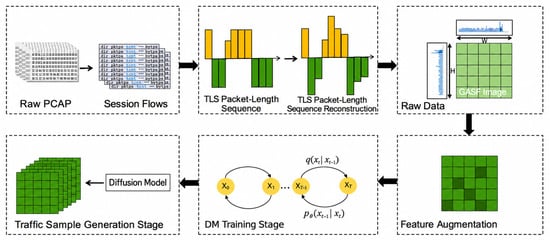
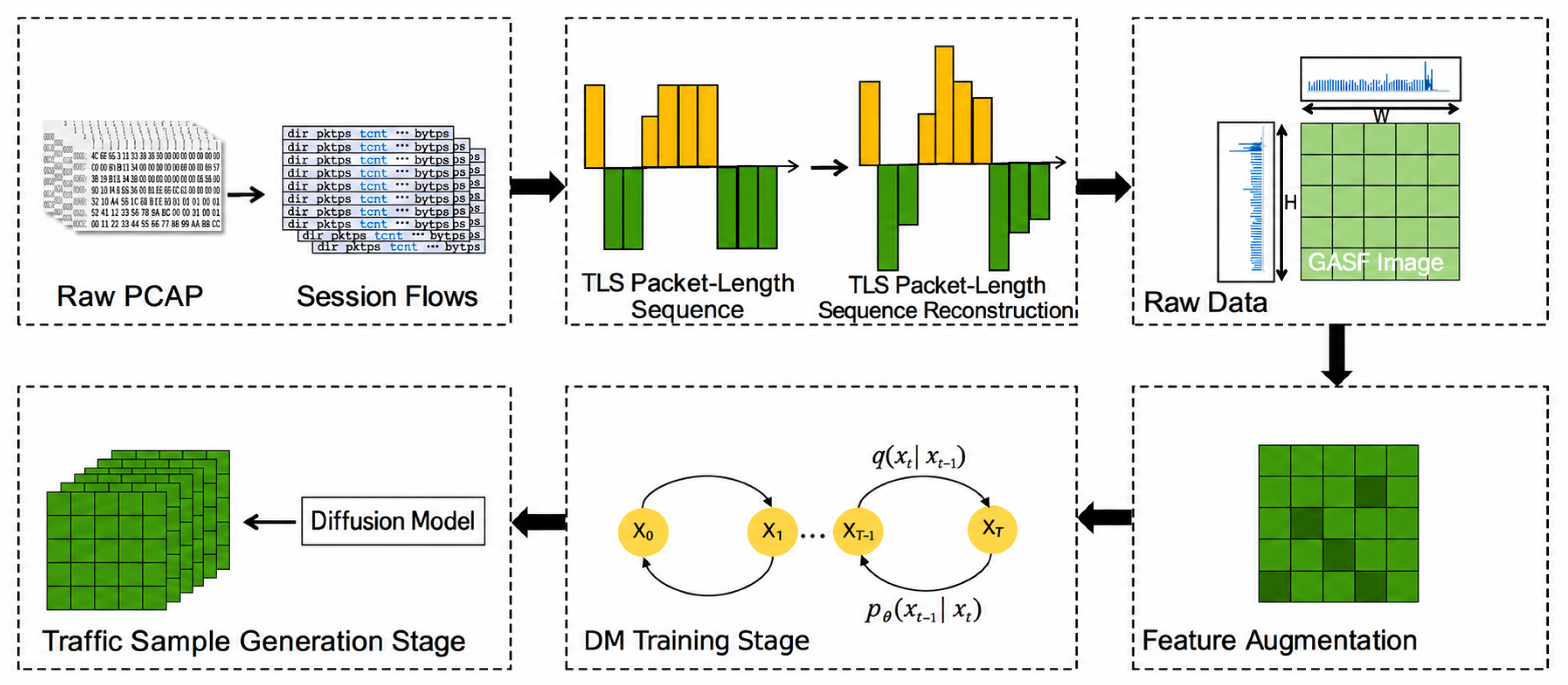
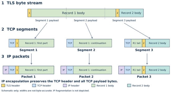
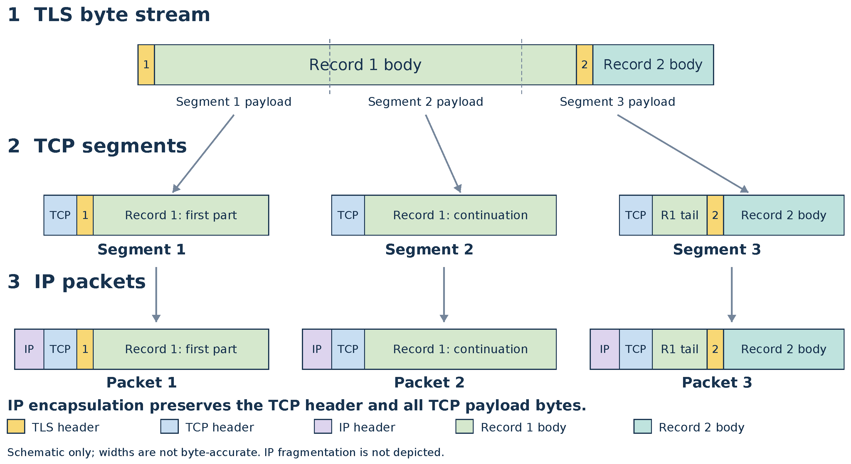
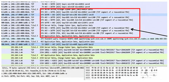
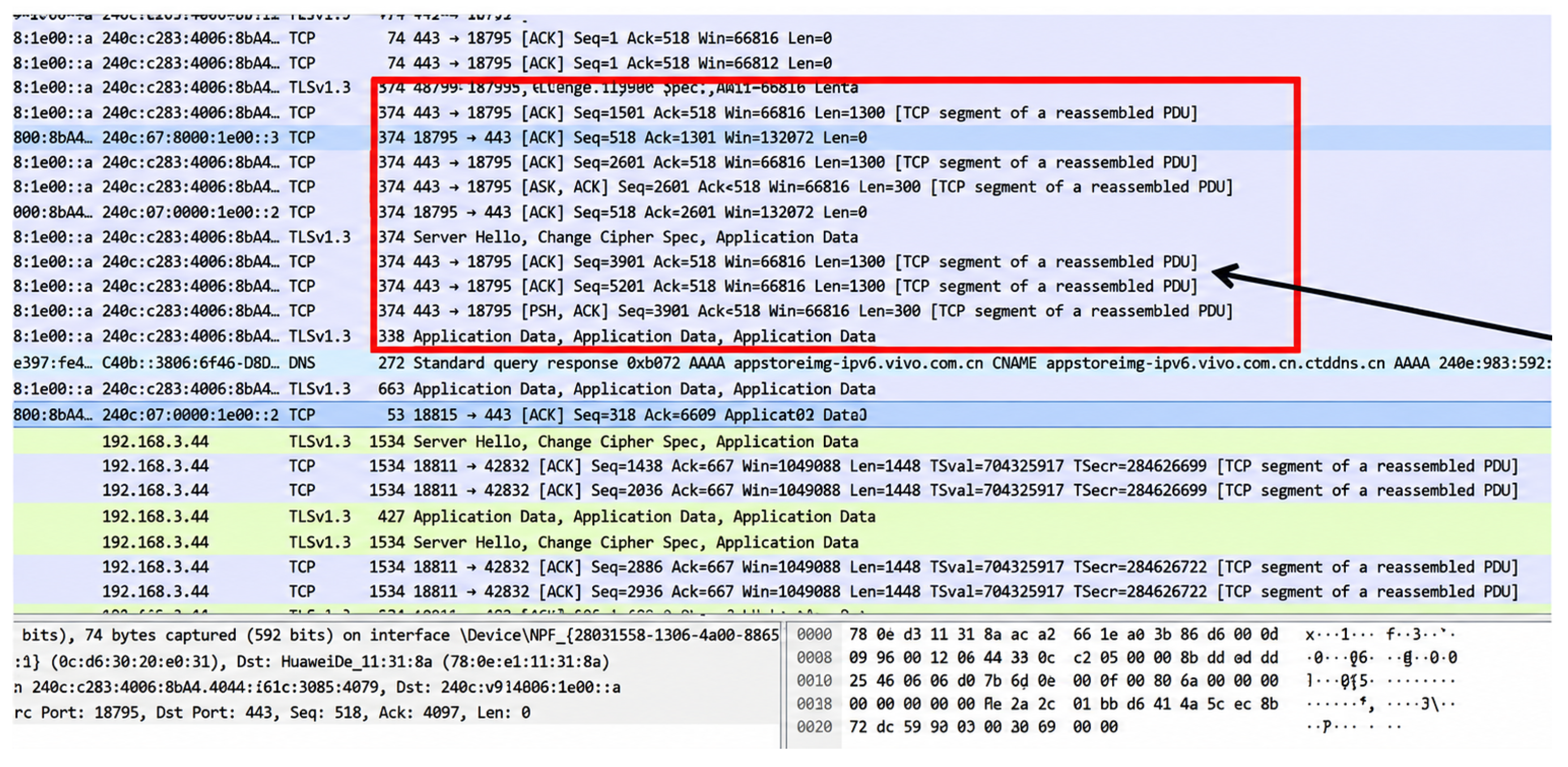
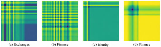
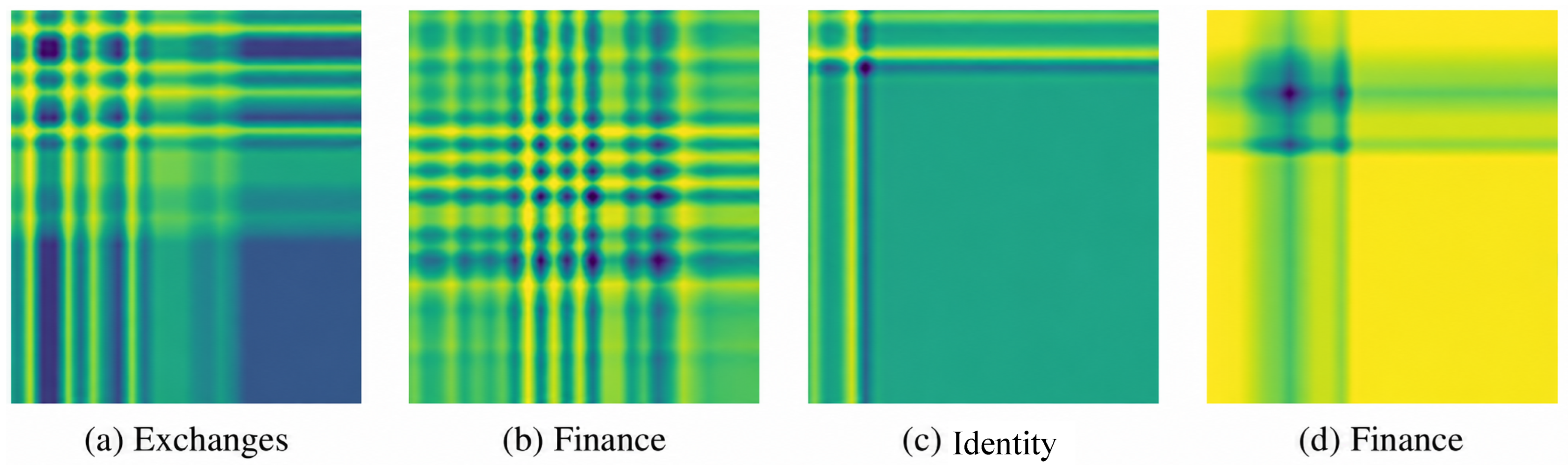
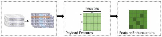
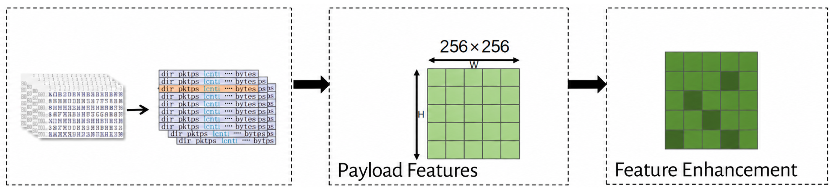
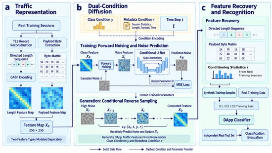
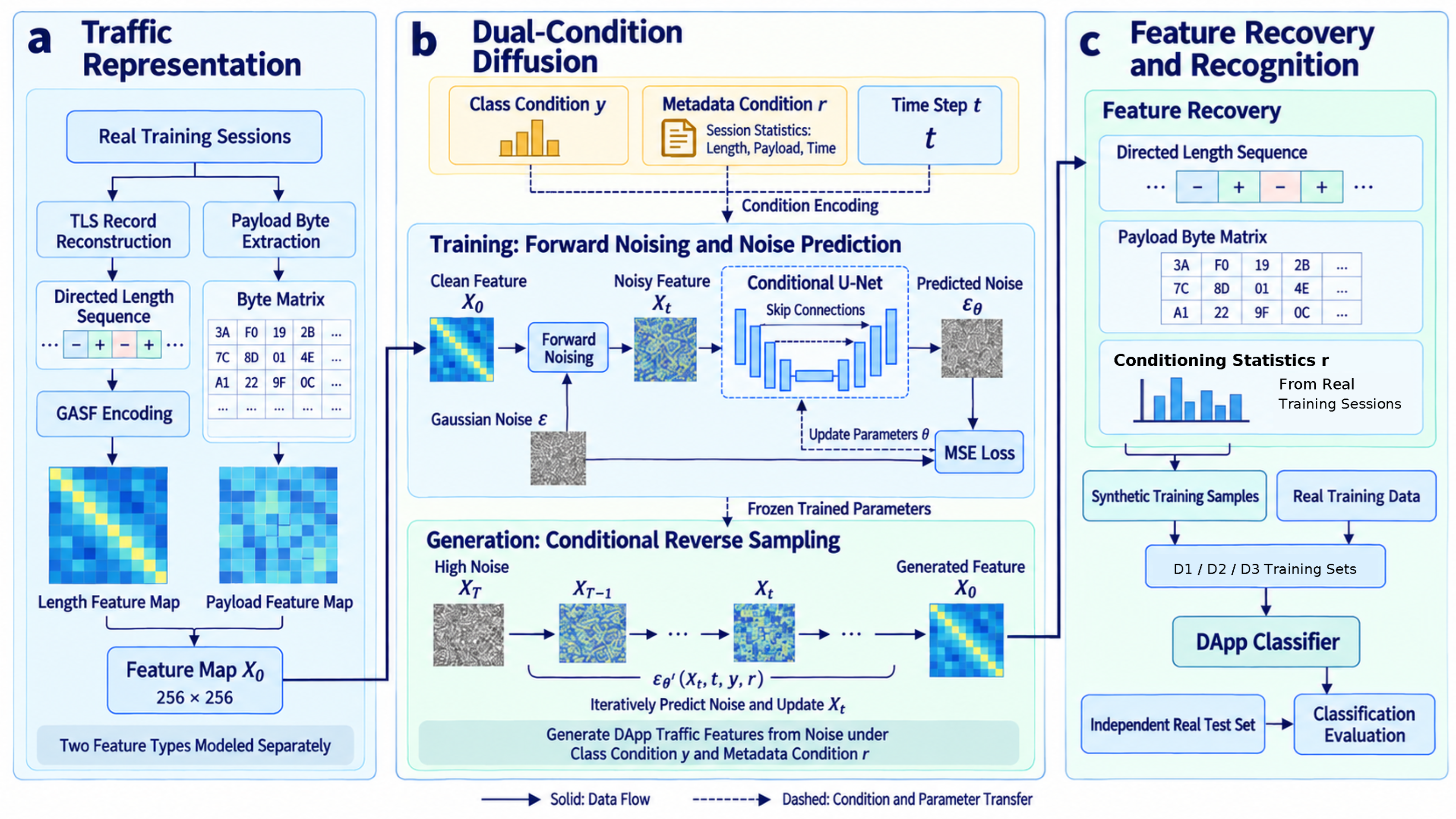
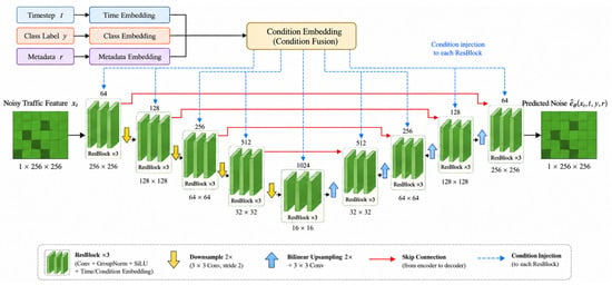
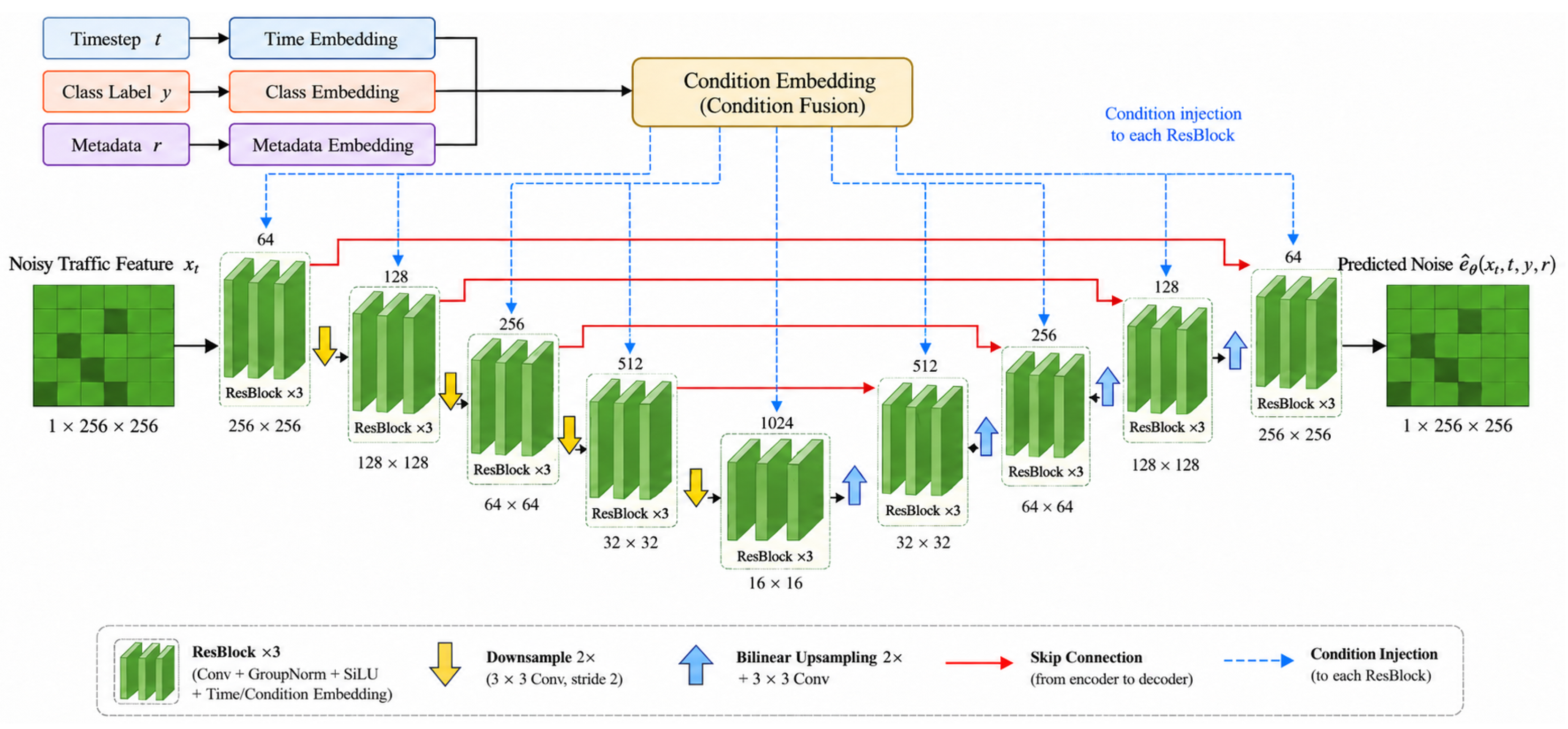
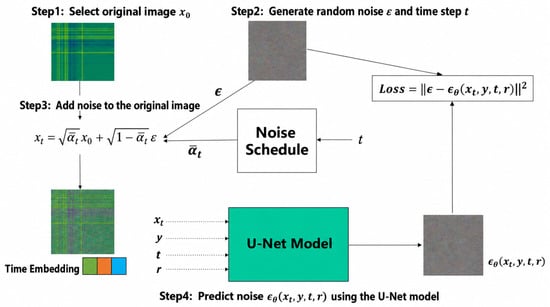
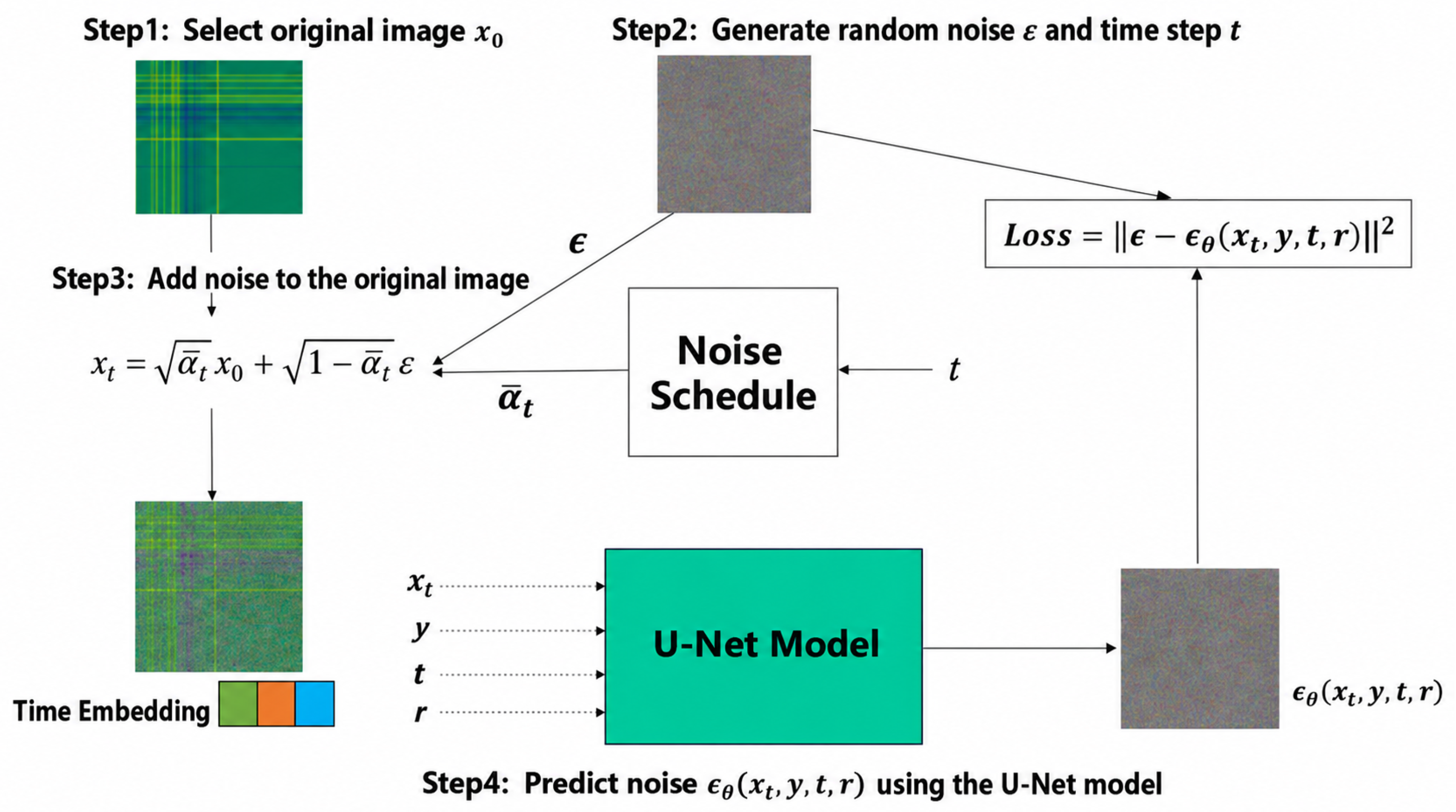
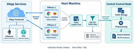
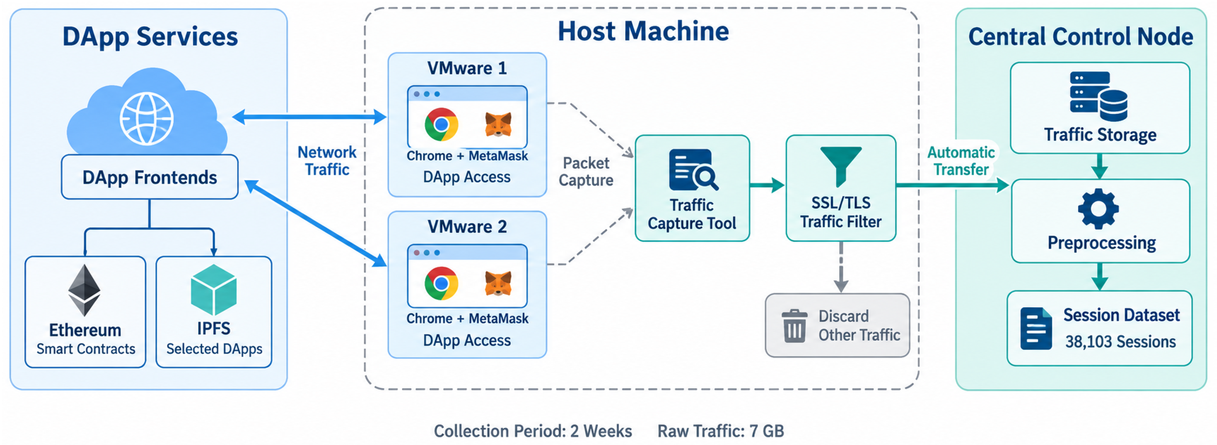
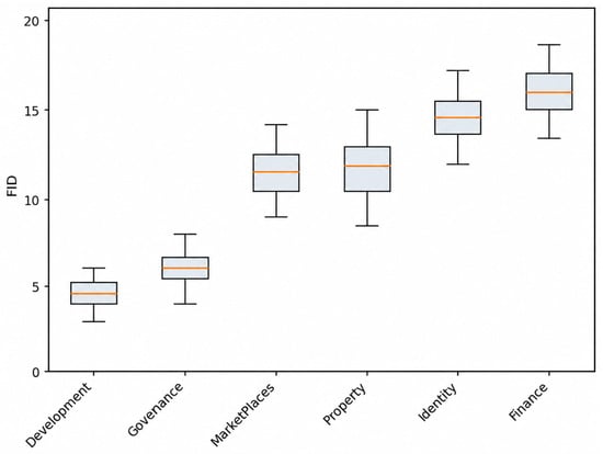
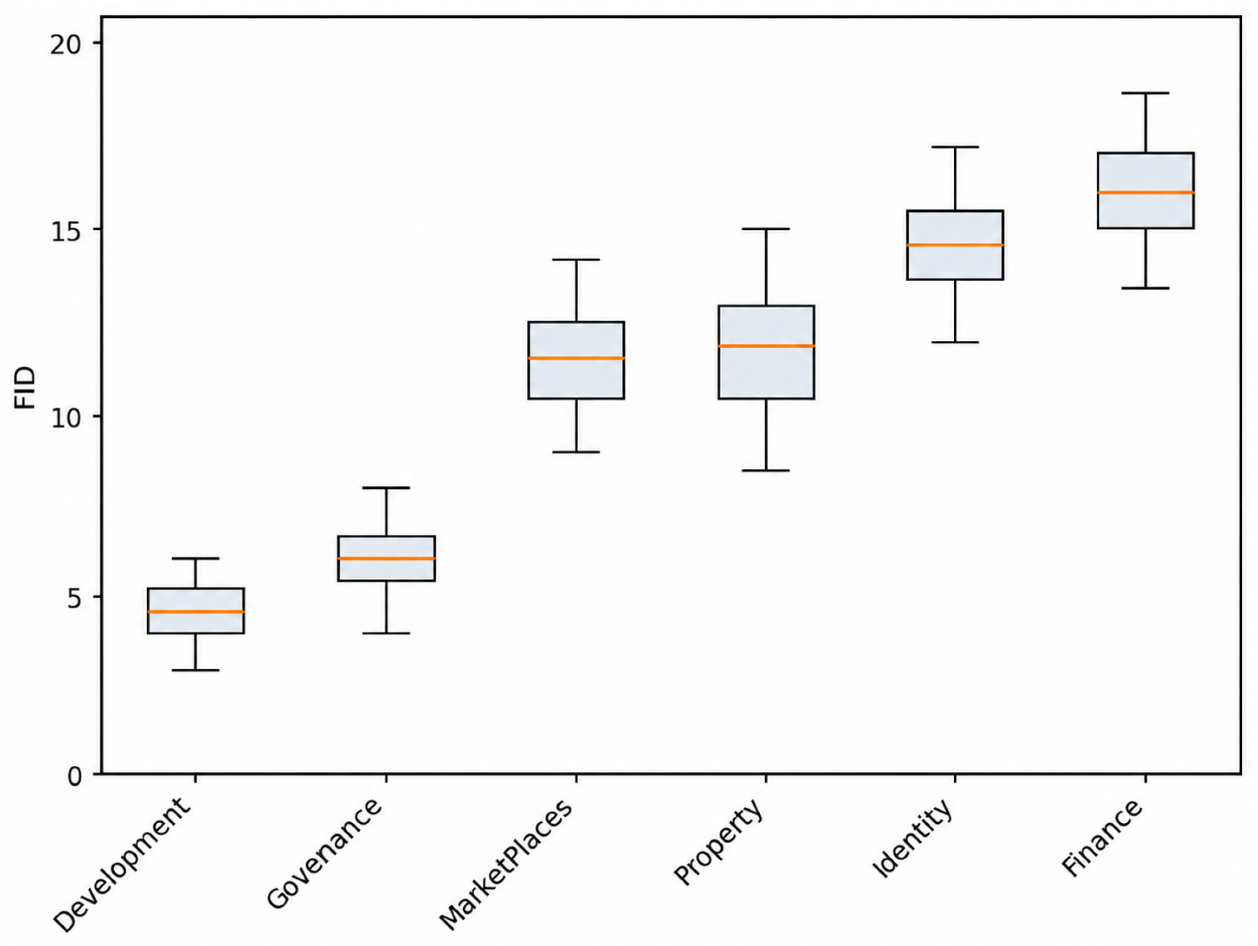
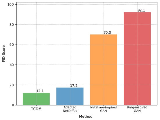
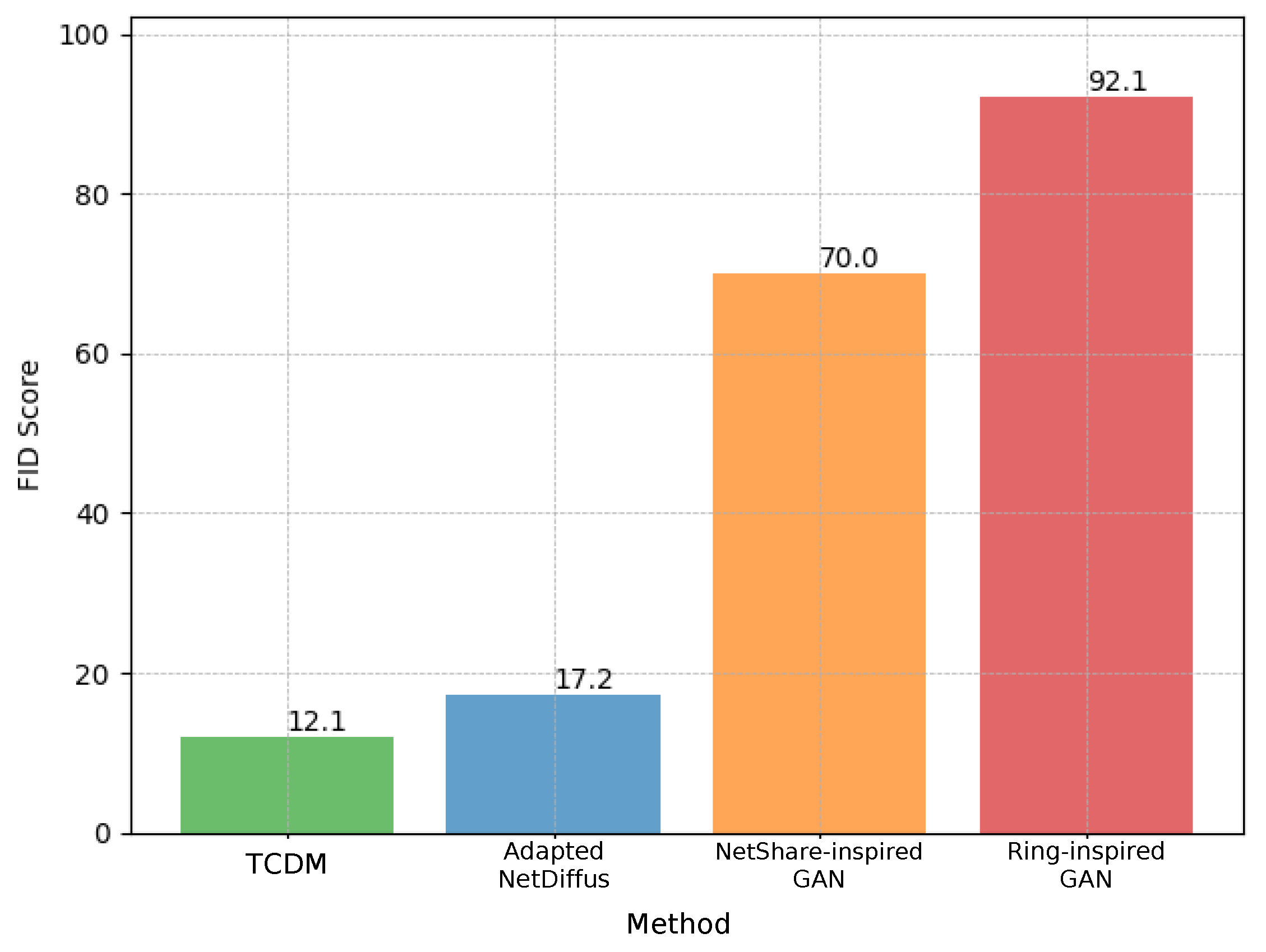
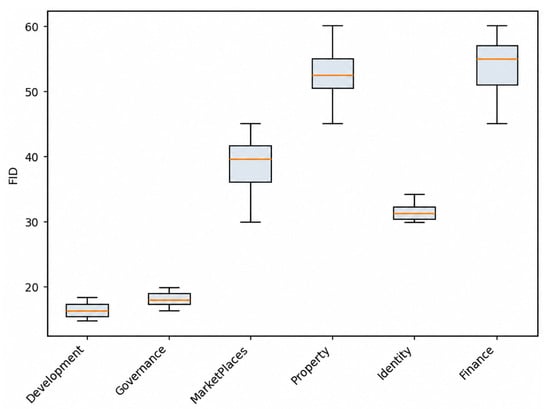
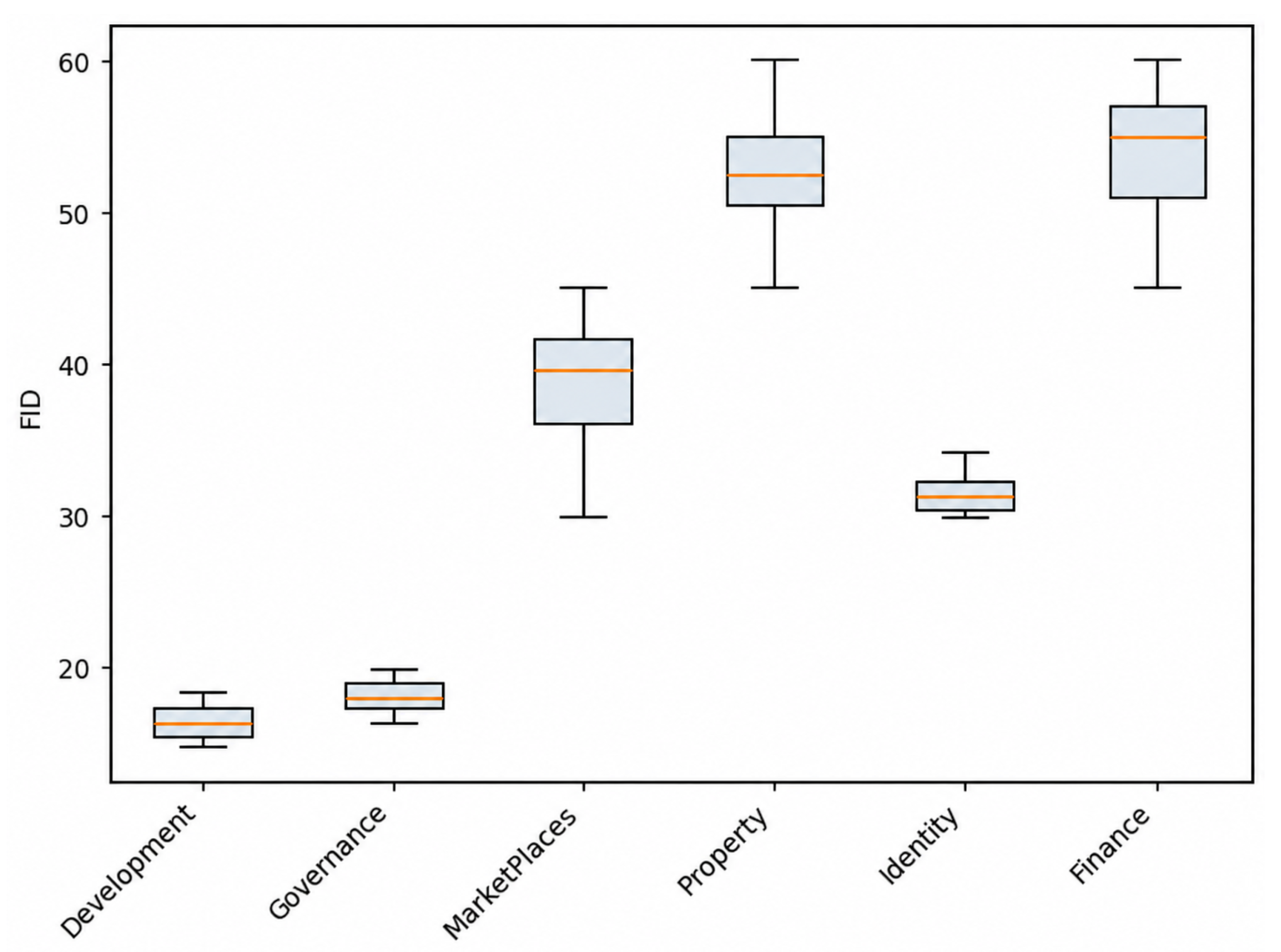
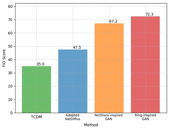
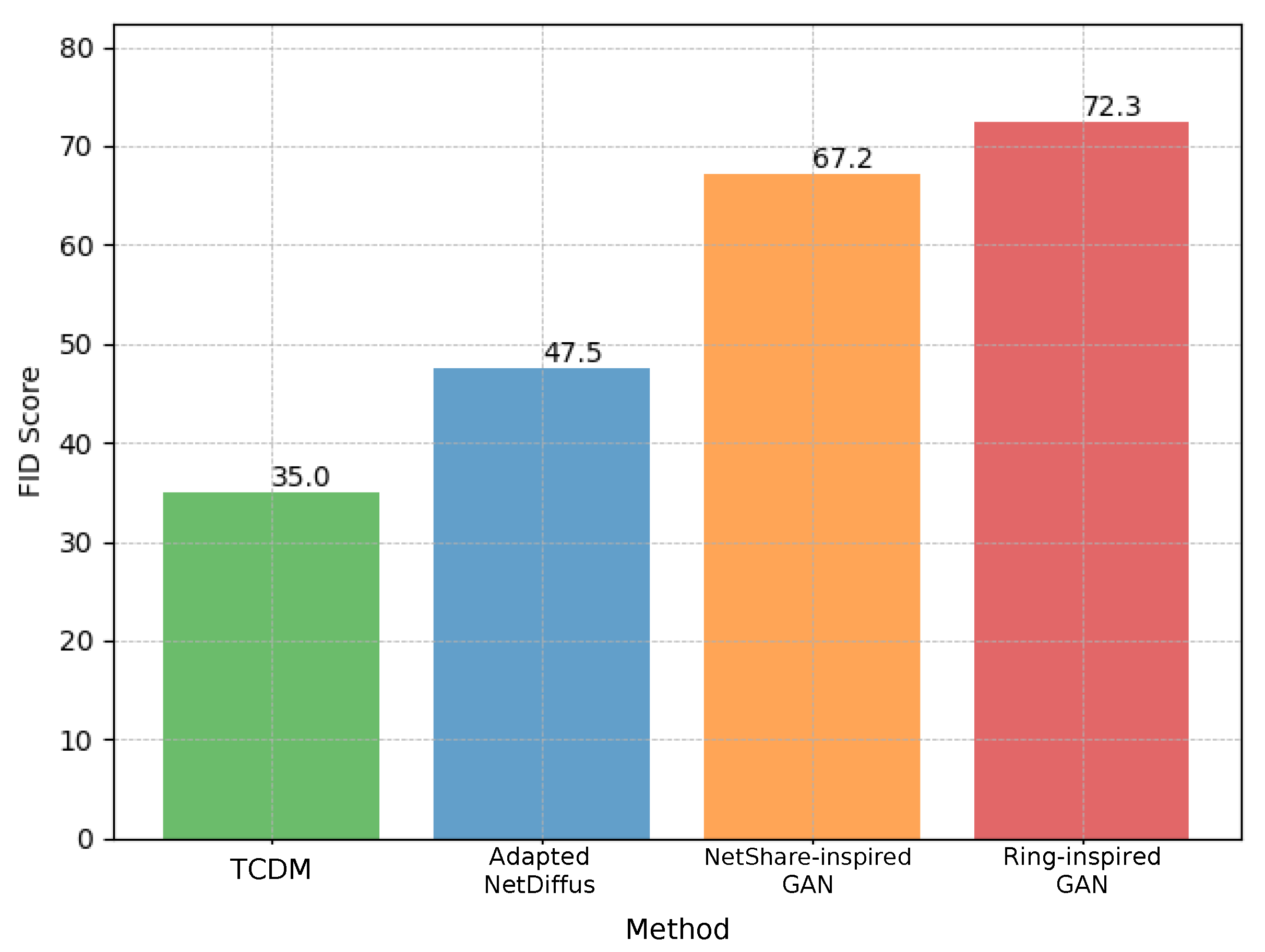
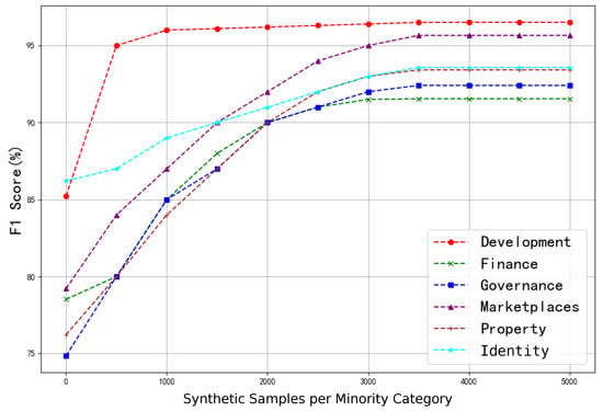
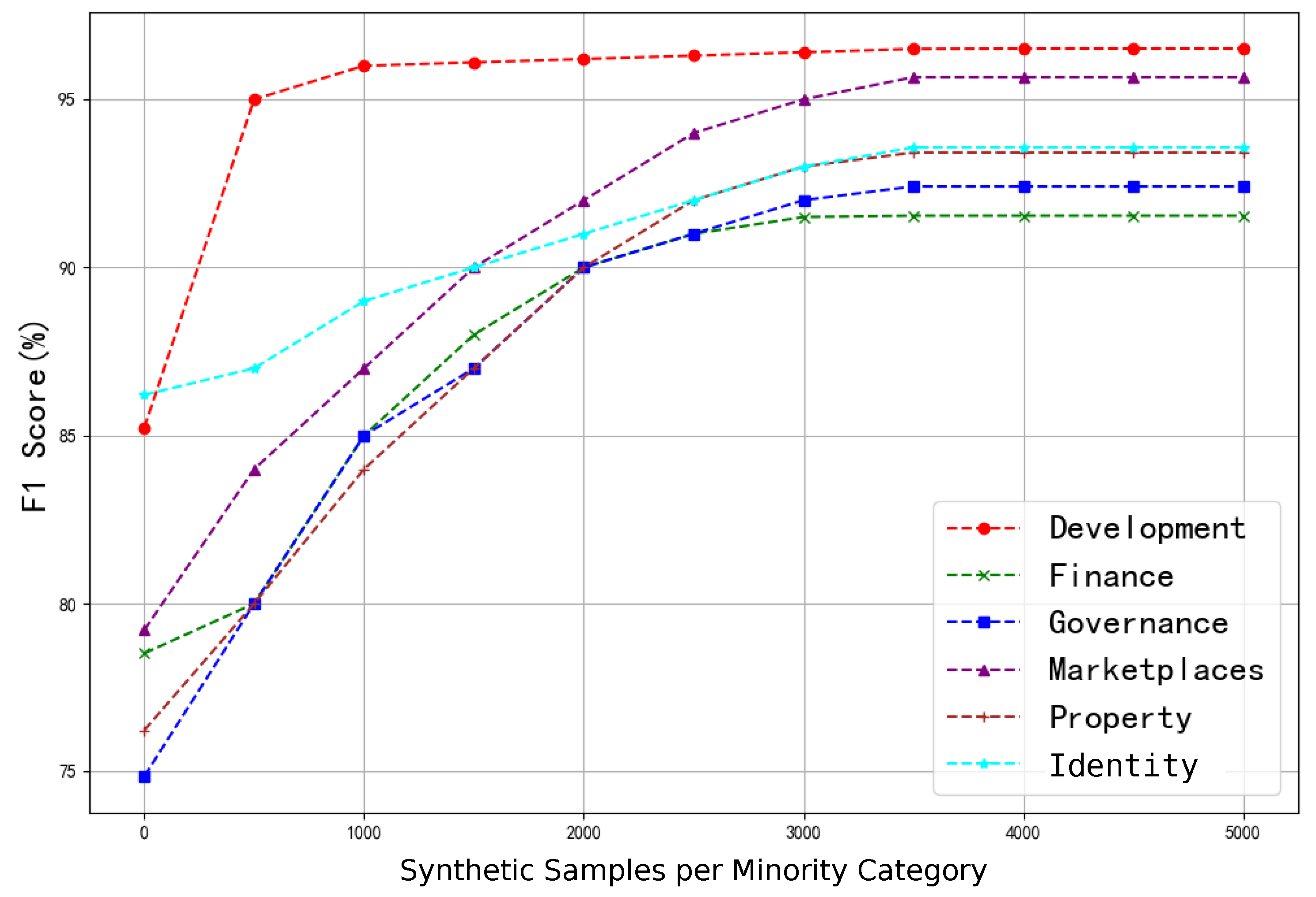
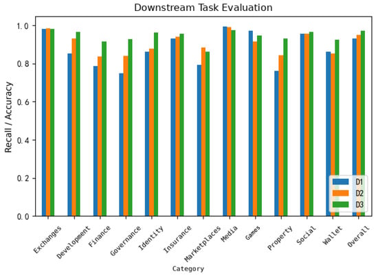
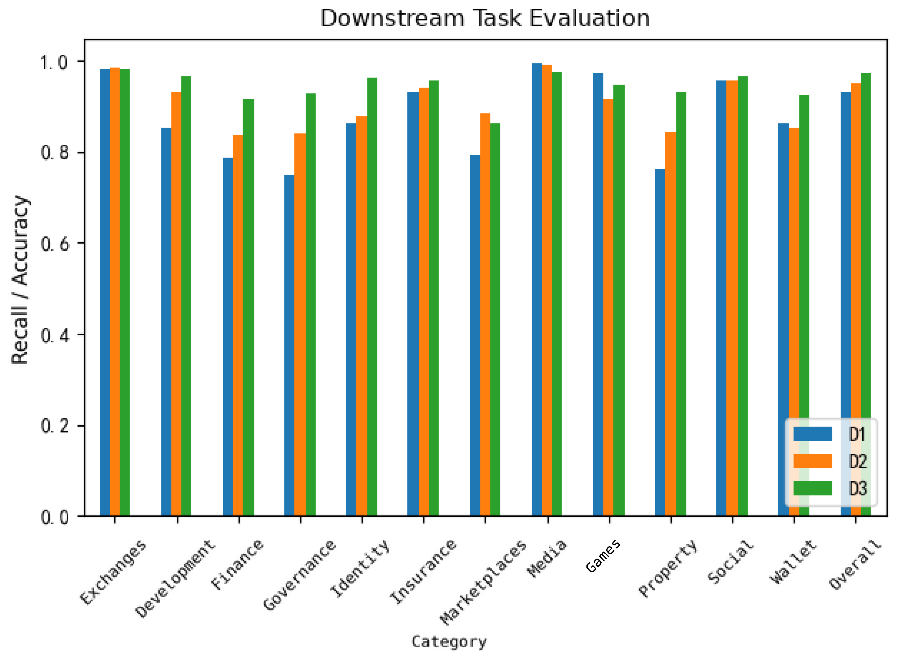

Disclaimer/Publisher’s Note: The statements, opinions and data contained in all publications are solely those of the individual author(s) and contributor(s) and not of MDPI and/or the editor(s). MDPI and/or the editor(s) disclaim responsibility for any injury to people or property resulting from any ideas, methods, instructions or products referred to in the content. |
© 2026 by the authors. Licensee MDPI, Basel, Switzerland. This article is an open access article distributed under the terms and conditions of the Creative Commons Attribution (CC BY) license.