


Abstract
In edge-computing-based distributed services, data traverse wireless multi-hop paths; when a link stays connected while loss and delay increase, route switching does not occur and a degraded route remains in use. Existing approaches predict degradation or locate faults but fix the recovery scope in advance. This paper proposes a route recovery scheme that sets the recovery scope from link-level fault identification aggregated into node-level confirmation, while a quality forecast screens the normal state before link-state collection. The scheme was compared with eleven other configurations on a 14-node wired testbed emulating wireless link loss and delay from distance and channel models. The faulty-link identification F1 score was 0.9822. In the window 30–60 s after degradation onset, throughput was 16.17–16.40 Mbps with the proposed scheme against 1.03–3.67 Mbps for the routing protocol alone. The protocol did not react under its fixed cost, nor did an RTT-aware cost calibrated on normal-state data. Recovery completed about 3 s later than with a threshold-based trigger, but no false recovery occurred before degradation onset in 56 cycles and a single-link degradation did not lead to node-level recovery. Replacing the forecast trigger with a measured-throughput rule, or removing the forecast features from identification, left the outcome unchanged.
1. Introduction
As the processing capability of edge devices has improved and the demand for real-time operation and service continuity has grown, computation for artificial intelligence services has increasingly been distributed across multiple devices [1,2]. The connections between distributed nodes form multi-hop paths that pass through intermediate nodes [3]. In wireless environments, path quality changes as links are created and lost, and each node acts both as an end device and as a router that relays traffic [4], so degradation in the quality of an individual link affects end-to-end service quality. Traffic between nodes is divided into large-volume data used for inference and delay-sensitive real-time streams, which are affected differently by the same link degradation. The inference data require sustained throughput, whereas the real-time streams require a bounded one-way delay and uninterrupted reception. A routing protocol that keeps a connected but degraded link in use restores neither, so meeting both requirements calls for a route recovery procedure separate from the protocol’s own route selection.
Among the routing schemes used to maintain such paths, distance-vector protocols compute link cost from the reception status of periodic control messages, so the cost does not directly reflect the throughput and delay observed in actual data transmission. When a link remains connected but loss and delay increase, route switching may not occur even though transmission performance has degraded [5,6], and it is difficult to locate, from link cost alone, where the degradation has occurred. Prior studies have predicted quality degradation to switch routes, or have identified fault locations [7,8,9,10,11], but the step from an identified fault location to a decision on recovery scope has not been sufficiently addressed, so the intervention scope is set without regard to the actual distribution of faults. We are not aware of prior work that aggregates the degradation of individual physical links at the node level to set the recovery scope and validates the result on a physical multi-hop testbed against protocol-only and threshold-based alternatives. The confirmation criterion is fixed, but the set of nodes it selects is not: it is formed at the time of the trigger from the paths then in use and from the link-level identification results.
This paper proposes a route recovery scheme that determines the timing of intervention from end-to-end quality prediction and sets the recovery scope according to the fault location obtained through link-level fault identification. The source node predicts future throughput from a time series of end-to-end quality metrics and, once a trigger occurs, collects link states from the nodes on both the forward and reverse paths. Each reported link is classified as faulty or not, the results are aggregated at the node level to confirm faulty nodes, and the links connected to a confirmed faulty node are blocked.
This paper makes four contributions. First, fault-location-driven recovery scope, with a link-level fallback for the nodes the criterion cannot confirm. Link-level identification results are aggregated per node and only nodes that meet the confirmation criterion are selected for recovery, so degradation of a single link does not lead to node-level recovery; in a single-link degradation scenario not seen in training, no node was confirmed as faulty in any of the 8 cycles, and in a further 10 single-link cycles with the link-level stage enabled that stage blocked the degraded link alone in 9 of them. The confirmed set held one or two nodes in the local scenario and, in the path-wide scenario, every degraded node except the one node with only two measurable links, and in 25 of the 56 cycles the degraded node lay only on the reverse path. Second, a physically validated multi-hop testbed. A 14-node testbed was built in which link loss and the degradation process are derived from distance and channel characteristics, and its measured transmission behavior was validated against theoretical models. Third, isolated evaluation of the prediction module. Prediction-based and measurement-based detection triggered at similar times, and the effect of prediction appeared in screening the normal state rather than in advancing the time of detection: over the 56 pre-degradation intervals of the proposed scheme, replayed on the recorded series, the prediction-based trigger fired in 7 intervals against 15 for a trigger on the measured throughput. Each of the seven was a single isolated sample, and no recovery procedure was issued in any of the 56 intervals. A 10-s moving median of the measured throughput removed these triggers entirely but detected degradation about 5 s later. The prediction module therefore combines a low rate of triggers in the normal state with the same detection time as the unsmoothed measured throughput: on the 40 protocol-only cycles the paired difference between the two triggers was 0.0 s [0.0, 1.0]. Replacing that trigger with the measured-throughput rule, with identification and confirmation left unchanged, did not change the recovery outcome: its throughput stayed within the confidence intervals of the proposed scheme and its trigger and recovery-completion times within 1.1 s, so what the prediction module contributes is the screening of the normal state, not the recovery result. Fourth, comparative validation of identification and recovery. The identification module reached an F1 score of 0.9822 against 0.9050 for the RTT-based rule, and among twelve configurations that differ in detection criterion and recovery scope, compared in the same testbed, the throughput in the common post-degradation window was 16.40 Mbps (local) and 16.17 Mbps (path-wide) with the proposed scheme, compared with 3.67 Mbps and 1.03 Mbps for the protocol-only configuration. Among these, a fixed path-wide recovery without identification was measured as a reference for the recovery scope, and the configuration whose identification module uses the seven hop measurements only, without the forecast features, confirmed the same nodes in all four scenarios and reached 16.40 Mbps and 15.32 Mbps in the same window, so the forecast outputs are not a condition for the end-to-end outcome.
2. Related Work
This section reviews prior work on path-quality degradation in ad hoc multi-hop networks in four categories: routing metrics that reflect link quality, degradation detection and rerouting, recovery-scope determination, and fault-location identification.
2.1. Link-Quality-Aware Routing Metrics
Routing protocols for multi-hop wireless networks have long incorporated link quality into their metric. ETX [6] and its multi-radio extension WCETT [12] estimate the expected number of transmissions from probe loss, OLSR applies link hysteresis to unstable neighbors [13], the airtime metric of IEEE 802.11s HWMP combines the transmission rate with the frame error rate [14], and Babel derives its cost from Hello reception [5]. These metrics react to the loss or delay of control probes rather than to the throughput and delay experienced by the data flows, so a link that still delivers probes but no longer sustains the traffic keeps a low cost, and a change in the metric moves the route without identifying which link caused the change. Link-quality estimation has also been treated as a learning problem, from estimators built on received-signal and loss statistics [15] to reinforcement-learning routing that selects the next hop from observed rewards [16,17].
Node-level exclusion is present in these protocols as well, but not as a decision on a set of faulty nodes: in OLSRv2 a neighbor takes the metric of its best link in the indicated direction among the symmetric one-hop links to it [18], so a node stays as good as its best link however many of its other links have degraded. Trust-based schemes do exclude whole nodes. Pang et al. [19] combine a direct trust score with a fuzzy evaluation of residual energy, packet transmission rate and one-hop neighbor count, and place a node whose score falls below a threshold on a blacklist broadcast to the whole network. Zhao and Srivastava [20] set the trust threshold according to the system environment and delete every node below it from the local trust list used for forwarding in a wireless mesh. In both, the input is a trust or misbehavior indicator, the quality of the physical links is not measured, and the evaluation is by simulation. All of these metrics and estimators choose routes, but they do not separate the decision of when to intervene from the identification of where the fault lies, which is the gap addressed in this paper.
2.2. Prediction-Based Rerouting
Several studies predict quality degradation and switch routes before a link breaks. Goff et al. [7] warned the source node when the received signal power fell below a threshold, prompting it to search for an alternative path, and Klemm et al. [21] used signal strength to assess the likelihood of disconnection and temporarily raised transmission power or switched paths. Gul et al. [8] predicted link-quality degradation with a decision-tree-based estimator, and Kavitha et al. [9] treated each node as a reinforcement-learning agent that predicted the likelihood of a link remaining available and used this prediction in next-hop selection. These studies use prediction results for path switching or next-hop selection but do not address how recovery scope should be determined according to fault location.
2.3. Recovery Scope
Recovery scope is divided into local recovery, which changes the path around the faulty segment, and global recovery, which searches the network for a new path; prior work defines the scope in advance according to the technique used. In the local-repair procedure of on-demand routing [22], the node immediately upstream of the broken link determines the search radius from the number of remaining hops, so the scope is set by the distance to the destination rather than by the location or cause of the fault. Lee et al. [23] had neighboring nodes that overheard a route reply maintain an alternate next hop, and Marina et al. [24] pre-established multiple disjoint paths so that switching could occur upon disconnection; both determine recovery scope from a predefined search range or alternate path and act on link disconnection. Wijesekara et al. [25] selected the minimum-delay or minimum-hop path according to congestion level from end-to-end path metrics, and Khudayer et al. [26] and Wang et al. [27] triggered path re-discovery or next-hop selection from link-quality prediction, with re-discovery covering the entire path from source to destination. Existing techniques thus predefine either a local or a global scope and do not determine it from the distribution of identified faults. Intervening at the node rather than at the link is the closer match when several links of the same node degrade together, as can happen when the node moves, its power supply weakens or an interference source lies beside it. Excluding one link at a time then leaves the route free to return to the same node, so recovery takes several rounds. The degradation applied here was injected on all interfaces of a target node, so it reproduces the condition but not its physical causes (Section 3.6). An isolated single-link fault is the opposite case, where the link is the right unit, and it is handled by the link-level stage that applies to the nodes the node-level criterion leaves unconfirmed (Section 3.4 and Section 5.3).
2.4. Fault Location Identification
Fault-location identification has long been studied in network diagnosis [28]. Srinivasan et al. [10] identified link disconnection and reconnection and estimated fault location from end-to-end delay, loss and flow rate observed passively at the entry and exit points of a path, and Feng et al. [11] proposed a network tomography technique that estimated upper and lower bounds on link performance even when it could not be determined directly from path-level observations. Harsh et al. [29] inferred switch and link fault probabilities in a large-scale data-center network with a Bayesian probabilistic graphical model, and techniques that structure anomaly detection and location identification as two stages have been validated in field deployments of optical transport networks [30,31,32]. These diagnostic studies apply fault location to root-cause analysis and do not carry the identified location into the determination of recovery scope. In software-defined networks the identification result does reach forwarding, but at the granularity at which it was obtained. Mostafaei et al. [33] give two mechanisms: one computes backup forwarding rules in the control plane in advance, and the other reads port liveness in the P4 data plane and sends the affected traffic to the next available port of the same switch. Both were tested on the BMv2 and Tofino software switches. Tao et al. [34] estimated per-link delays from end-to-end measurements between monitor pairs, approximating the links that the measurements cannot identify, and selected one whole path per pair with an upper-confidence-bound rule, without excluding any link; in the NSF-like topology they deployed on a testbed, 54.5% of the links were identifiable with monitors on 60% of the nodes. Identification at the port or the link is therefore not aggregated into a set of faulty nodes, and the recovery scope is either the next available port or a learned path.
2.5. Summary and Positioning of This Paper
Prior work has addressed link-quality-aware metrics, degradation prediction, recovery-scope setting, and fault-location identification separately. Prediction-based techniques determine when to intervene, recovery techniques change the path within a predefined scope, and diagnostic techniques identify fault locations. Node-level exclusion exists in the trust-based schemes, and localization results are carried into forwarding in software-defined networks, but we are not aware of prior work that aggregates the degradation of individual physical links at the node level to set the recovery scope and validates the result on a physical multi-hop testbed. This paper sets the recovery scope from link-level fault identification aggregated at the node level, and uses an end-to-end quality forecast to screen the normal state before link states are collected. The differences are summarized in Table 1. Because wireless multi-hop environments are difficult to test repeatedly under identical conditions and few proposed schemes have been validated in real deployments [35], the scheme is evaluated on a testbed that separates the transmission medium of each hop, corresponding to a multi-radio mesh with orthogonal channels [12] rather than to a single-channel network whose capacity decreases with hop count [36,37].
Table 1.
Comparison of related work: degradation detection criterion, faulty-link identification, and the basis for deciding the recovery scope.
3. Materials and Methods
In this paper, a faulty link is defined as a link whose transmission quality has left its normal range while connectivity is still maintained. Three terms are used throughout: a degraded link or node is one to which degradation was applied in an experiment, a faulty link is one that the identification module classifies as such, and a confirmed faulty node is one that satisfies the node-level criterion in two consecutive rounds and thus becomes the recovery target. The proposed scheme determines when to intervene through end-to-end quality prediction, confirms faulty nodes through link-level identification followed by node-level aggregation, and sets the recovery scope according to the distribution of the confirmed faulty nodes.
3.1. System Overview
End-to-end quality metrics observed at the source node summarize the whole path in a single value, so even when degradation is detected, the location of the fault cannot be identified directly, and replacing the whole path without this distinction can alter segments that are operating normally. The proposed scheme was therefore designed as a sequential two-stage structure: end-to-end quality prediction determines when to intervene, and link-level identification then determines the fault location and the recovery scope. The overall architecture is shown in Figure 1.
Figure 1.
Overall architecture of the proposed scheme. (a) Prediction-triggered fault identification and recovery. (b) Prediction module.
In the first stage, the source node measures throughput, round-trip time (RTT), RTT variation (jitter) and the number of retransmissions every 1 s, accumulates them as a time series, and feeds this series to the prediction module, which forecasts future throughput. When the predicted value falls below a preset threshold, the module raises a trigger that starts the link-state identification of the second stage.
The source node sends the trigger toward the destination node, and the destination node sends the same trigger back toward the source node. In distance-vector routing protocols, the forward and reverse paths can differ when several candidate paths have equal cost, so the trigger is propagated in both directions to collect the state of the links on each directional path. Each node through which the trigger passes reports its own link states to the source node. The identification module decides whether each link is faulty and aggregates the link-level results per node to determine the recovery scope. Because the link states used in the earliest rounds may not yet fully reflect the degradation, identification is repeated at every identification round, and recovery is executed only when the same faulty-node set has been confirmed in consecutive rounds.
3.2. End-to-End Quality Prediction
The input to the prediction module consists of four metrics: throughput, RTT, jitter and the number of retransmissions. At each 1-s step, the 24 most recent samples are taken in a sliding window to form the input sequence. Jitter and the retransmission count were added because throughput and RTT alone do not adequately capture the range of changes in end-to-end quality. The inputs used by the prediction and identification modules are listed in Table 2.
Table 2.
Input configuration of the prediction and identification modules.
Signs of degradation may lie in the pattern of change over an interval rather than in the value at any single instant. PatchTST [38] was therefore adopted; it divides the input time series into fixed-length patches and uses each patch as an input token to a Transformer encoder. The input sequence was split into non-overlapping patches of four samples each, yielding six patches from the 24 samples, with each patch covering a 4 s interval, and the encoder was given a lightweight structure with real-time inference in mind. The representations of the individual patches were averaged into a single feature vector for throughput prediction, as shown in the enlarged inset of Figure 1.
Because the uncertainty of the prediction must be considered together with the predicted value under changing wireless conditions [39], quantile regression [40] was applied to predict throughput 1, 2, and 3 s ahead at the quantile levels of 0.1, 0.5 and 0.9. The model was trained with the pinball loss [40,41] in Equation (1), where y is the observed value, is the predicted value and is the target quantile, and the final loss was the mean of the nine losses over the three horizons and three quantiles.
Here h is the prediction horizon in seconds, t is the current 1-s sampling step, is the throughput observed at step and is the corresponding prediction at quantile ; the two throughput terms and are in Mbps, and is dimensionless.
The difference between the upper and lower quantiles was defined as the width of the prediction interval and used as an indicator of prediction uncertainty. The median-quantile prediction and the prediction-interval width at each horizon were used as input features to the identification module.
A trigger is raised when the median-quantile prediction of throughput 3 s ahead is below 10.0 Mbps. Samples within 3 s of flow start were excluded, and the trigger decision was applied only once the input sequence had been filled with 24 valid samples. The 10.0 Mbps threshold lies about 4.4 standard deviations (1.726 Mbps) below the mean end-to-end throughput of 17.618 Mbps measured over the baseline intervals of the training cycles. The normal-state throughput is not normally distributed, however: it has a heavy lower tail of transient dips, so the measured throughput still fell below the threshold in 15 of 56 pre-degradation intervals (Section 4.2), and the threshold should be read as a level to which the sustained throughput does not fall in the normal state rather than as a probabilistic bound. Because throughput can drop below the threshold temporarily even in the baseline interval, the trigger decision uses predicted rather than currently measured throughput.
3.3. Link-Level Fault Identification
The identification module operates after a trigger is raised and computes a fault probability for each link whose state information was collected along the forward and reverse trigger paths. Its input comprises 14 features: seven state metrics collected on each link, six outputs of the prediction module and one conflict score, as detailed in Table 2. The prediction outputs let the input reflect the predicted end-to-end quality as well as the current link state, and the conflict score quantifies the gap between the two.
As given in Equation (2), the conflict score is the difference between the mean end-to-end throughput over the preceding samples and the median-quantile prediction of throughput 3 s ahead, where is the end-to-end throughput measured at time k and is the median-quantile value predicted at the current time t. A larger conflict score means that the predicted throughput is lower relative to the recent mean.
The quantities , and are in Mbps, and W is a number of 1-s samples.
As given in Equation (3), the link loss rate is the number of packets dropped in the preceding 10 s divided by the number of packets sent in the same interval, where and are the cumulative dropped and sent counts up to time t. The 10 s interval gives a stable loss rate, and the normalization makes loss comparable across links carrying different traffic volumes.
The counts and are numbers of packets, W is in seconds and is a dimensionless ratio.
Each link is treated as an independent sample represented by a fixed-length vector of the 14 features and classified by LightGBM [42], a gradient-boosted decision tree method. Node and interface identifiers were excluded from the input so that the fault decision rests on the observed link state rather than on the identity of a particular node. The classifier outputs the fault probability of each link; a link is judged faulty if its probability is 0.6 or higher, normal if it is below 0.5, and undecided otherwise. Undecided links are not counted as faulty links in node-level aggregation, so in Algorithm 1 is true only for .
| Algorithm 1 Faulty-node confirmation and route switching. |
|
3.4. Faulty-Node Confirmation and Route Recovery
The recovery scope is determined from the set of nodes judged to be faulty. As given in Equation (4), the link-level results are aggregated per node, and a node is confirmed as faulty when both the ratio and the number of its faulty links meet the preset criteria. is the number of links at node n judged faulty, and is the number of measurable links at that node, that is, the links attached to it excluding those directly connected to the source or destination node. The ratio criterion and the count criterion k were set to 0.75 and 3 respectively, and F is the set of faulty nodes satisfying both conditions. The two criteria were combined because either alone could be dominated by a node with very few or very many links; both were fixed before the experiments. Under the count criterion, a node with fewer than three measurable links is never confirmed as faulty, and degradation of a single link cannot by itself cause a node to be confirmed as faulty.
Confirmed faulty nodes are removed from the route by the same procedure regardless of their number, so the recovery scope follows the number and distribution of the confirmed nodes. The recovery procedure consists of two steps. First, the links attached to the faulty node are blocked at both ends, which removes the node from the set of routing candidates; blocking at only one end would leave the neighbor relationship intact at the other end and delay the route switch. Then, if the faulty node is the forward next hop of the source node or the reverse next hop of the destination node, the source node or the destination node, respectively, assigns one of its neighbors other than the faulty node as a temporary next hop. The next hop is assigned at both ends because changing only the source node’s next hop leaves the reverse path traversing the degraded segment. The temporary next hop is released once the routing protocol has installed a route that bypasses the faulty node and reachability to the destination has been confirmed four consecutive times at 0.5 s intervals, or otherwise 15 s after it was assigned.
The links are blocked directly rather than by raising their cost, because a cost increase cannot guarantee a lasting exclusion as load changes. Blocking is a link-layer action: the source node floods the identities of the confirmed nodes in a UDP control message, and every node that receives it disables its own interface toward a confirmed node, so a link is removed at both ends without relying on delivery of the message to the faulty node itself. On the pairwise segments of the testbed this removes exactly one link; on a shared wireless interface the equivalent action would be a per-neighbor blacklist rather than an interface shutdown. A link-down event is itself visible to the routing protocol, which is why the comparison configurations of Section 3.9 apply the same blocking action with a different scope, so that the effect of the detection criterion and of the scope can be separated from the effect of the blocking action. No procedure for reactivating blocked links is included; the conditions and timing of restoration are outside the scope of this paper.
An optional stage covers the nodes that the confirmation criterion does not confirm. Within a trigger that confirmed no node, or that confirmed some nodes while leaving others undecided, the links of the undecided nodes are then examined one at a time: a link whose fault probability has stayed inside the faulty band of Section 3.3 for N consecutive identification rounds is blocked at both ends, and no other link of the same node is touched. N depends on what else the same trigger produced, 2 when a node was confirmed in it and 8 when none was, because node recovery ends identification after about two rounds in the first case, whereas identification continues in the second and a longer run of rounds is available. Two guards restrict the stage: the link facing the destination is never blocked, and a link whose removal would disconnect the source from the destination in the current topology is refused. The stage reads nothing about where degradation was injected, so a block issued before degradation onset is carried out and counted like any other. The agents are unchanged, since the source node names one link end as faulty and the remaining ends of that node as to be kept, and each node applies the rule it already uses for a confirmed node.
The full procedure, from fault-probability computation to route switching, is given in Algorithm 1. A link-state report is excluded from the decision input if more than 2 s have passed since its last update. Link decisions and node-level aggregation are repeated at every state-reporting interval; when the same set of faulty-node candidates is observed in two consecutive identification rounds, that set is confirmed and the recovery procedure is executed. If no faulty node has been confirmed within 30 s of the trigger, identification ends and no route switch is performed.
The computation of the prediction stage is independent of the path, whereas that of the identification stage grows with the number of reported links L, the number of reporting nodes N and the number of identification rounds R until confirmation, as given in Equation (5): each round classifies the L reported links once and aggregates them over the N nodes once. R is at least 2 and is bounded by the decision time limit of 30 s after the trigger.
Here is the cost of one identification round and the cost until confirmation, both expressed as counts of link classifications and node aggregations; L, N and R are counts.
3.5. Testbed
A physical testbed that emulates the link structure of a wireless multi-hop network over wired connections was built from 14 Raspberry Pi 4B units interconnected by Ethernet. A virtual switch and VLAN tagging formed an independent transmission segment for each node pair, and netem [43,44], the kernel’s traffic-control facility, was applied to each virtual interface to reproduce link-quality degradation and packet loss. Because each link has its own transmission medium, the contention of a single shared channel [36,37] is not emulated; the testbed corresponds to the link-separated structure of a multi-radio wireless mesh [12].
The testbed topology is shown in Figure 2. The 14 nodes were connected by 27 bidirectional links. The path between the source node and the destination node was a 4-hop path through three intermediate nodes, and several alternative paths were provided so that a faulty segment could be bypassed. End-to-end metrics were measured at the source and destination nodes, link-state collection agents were deployed on the 12 intermediate nodes, and prediction and identification were performed at the source node. The delay and loss used to reproduce link degradation were applied in the transmit direction of the 48 interfaces that form the inter-node links at the intermediate nodes.
Figure 2.
Testbed topology.
Babel [5], a distance-vector protocol, was used for routing. Babel exchanges control messages periodically with its neighbors and reflects their reception in the link cost [45], so the link cost does not necessarily match the changes in throughput or delay observed in data transmission. The Hello interval was left at its default of 4 s, and no interface receive-cost adjustment was applied. Because the interfaces are Ethernet ports, babeld treats them as wired links and assigns a fixed cost to a neighbor as long as Hello messages are received, so neither packet loss nor delay on the data path enters the link cost. The wireless-type cost of babeld, which scales with the Hello loss ratio, was measured rather than estimated: with the interfaces declared wireless, a dump taken during degradation in each of the 40 cycles showed a median neighbor cost unchanged at the baseline value of 256 (a change of 0.0%). Of 935 cost samples, 29 rose by more than 1% (by at most 33.2%), including 23 of the 546 samples at neighbors of the degraded nodes. No new route was installed at the source node in any of the 40 cycles and the hop count was unchanged in all of them, so the loss-sensitive cost function moves the cost of some links without changing the route. The dump could not be collected at the source node, so its own neighbor costs are not included. babeld can also derive a third cost from delay: with the delay-based metric extension [46] the two neighbors of a link timestamp their control messages, and the link cost receives a penalty that rises linearly with the smoothed round-trip time from zero at rtt-min to max-rtt-penalty at rtt-max. The protocol-only configuration is evaluated under the fixed wired cost, and the same configuration with the wireless-type cost and with a calibrated RTT-aware cost is evaluated separately (Section 3.9 and Section 4.4). A fixed path-wide recovery without identification is examined as a reference configuration in Section 4.6. The bandwidth of every link was capped at 19,232 kbit/s, a value set from the effective capacity of an 802.11g environment so that the physical capacity of the wired segments is not reflected directly in end-to-end throughput. The rate cap was applied above the loss and delay settings and held constant throughout degradation, so that changes in link state appear through loss and delay rather than through the rate limit. All 14 nodes shared the same reference time, with a clock offset below 1 ms, so that one-way delay could be computed.
The experimental traffic consisted of a TCP-based bulk transfer and a UDP-based real-time stream. The bulk transfer was a single iperf3 TCP flow maintained for 170 s in each cycle with kernel-default congestion control; throughput was measured at the receiver every 1 s and joined with the sender’s TCP state (RTT, jitter and retransmissions, collected every 0.5 s) to form a time series at 1 s resolution. The real-time stream was a constant-bit-rate UDP flow of 200 packets per second with a 1250-byte payload, sustaining 2.0 Mbps; the first 16 bytes of each packet carried a sequence number and a send timestamp, the receiver logged every packet, and a deadline miss was declared when the one-way delay exceeded 150 ms. In the system comparison experiments, the two flows were transmitted simultaneously. Link-state reports are carried to the source node over the same network as the data traffic; the collection agent on each node reports per-interface state every 1 s, and only after a trigger has been raised.
3.6. Degradation Model
To reflect the basic delay and loss characteristics of a wireless environment even without degradation, background delay and background loss were applied in the transmit direction of all link interfaces of the 12 intermediate nodes, drawn independently from uniform distributions for each link and each cycle. Background loss was set from a transition probability range of 0.0011–0.034% (average loss rate of about 0.003–0.102%), obtained by applying inter-node distances of 1–5.65 m to a propagation model, and per-hop one-way delay was set in the range 2500–6500 s with reference to delay distributions measured in real wireless networks [47]. The same background conditions were applied in all scenarios, and additional degradation was applied to the target nodes in the local and path-wide scenarios.
Five degradation scenarios were defined: baseline, local, path-wide, delay-only and single-link. The baseline scenario applies only background delay and loss and was used to build training data and to evaluate false detections under normal conditions. In the local scenario, degradation was applied to the middle relay node of the forward and reverse paths; in the path-wide scenario, all relay nodes on both paths were degraded. The same degradation was applied to all link interfaces of a target node, and the target nodes were selected in each cycle from the observed forward and reverse paths rather than fixed by node identifier. The delay-only scenario, which increases delay without changing packet loss, and the single-link scenario, which degrades only the transmit interface from the middle relay node of the forward path to its next hop, were defined to check generalization to conditions not included in training. A loss-only scenario, the counterpart of the delay-only scenario, was collected later in 10 additional cycles in which the local loss profile was applied while the background delay was held fixed; these cycles were recorded without recovery actions and are used only in Section 4.3.
In the local and path-wide scenarios, loss and delay were raised every 1 s from each link’s background values to the final settings of the scenario. The temporal profile was generated from the change in propagation characteristics under the assumption that the link distance increases at a constant rate; it does not emulate actual node movement, and attenuation by obstacles and interference were not modeled. As given in Equation (6), the inter-node distance at time t is , where is the background distance of the link and v is the rate of distance change. The path loss is computed with the log-distance path loss model [48], the mean received power is obtained from the transmit power and the path loss, and the difference between the mean received power and the receiver sensitivity [49] defines the fading margin , from which the outage probability (reception-failure probability) is computed under Rayleigh fading. The degradation progress is the normalized extent to which the reception-failure probability has moved from , the reference value at the upper bound of the background range, toward , the value corresponding to the final setting; it remains constant once the final setting is reached. The same progress was applied to loss and delay. The model parameters are listed in Table 3, and the evolution of degradation over time is shown in Figure 3.
Figure 3.
Derivation of the degradation waveform and its evolution over time.
In Equation (6), and are in meters, v in m/s and t in seconds; is the path-loss exponent, f the carrier frequency in Hz, c the speed of light in m/s and m the reference distance; is in dB, , and are in dBm and the fading margin is in dB; , , and the degradation progress are dimensionless and lie in . The values of , f, , and v are listed in Table 3.
Packet loss on wireless channels concentrates in short time intervals, which a model with independent per-packet loss cannot reproduce. A two-state Markov (Gilbert–Elliott) loss model [50,51] was therefore applied, with p the transition probability from the good state to the bad state and r the recovery probability from the bad state to the good state; all packets are dropped in the bad state, so the mean loss rate at equilibrium is the occupancy probability of the bad state, as given in Equation (7). During degradation, r was held at 33.3% while p was raised with the degradation progress, and in the path-wide scenario r was changed to 50.0% when the final setting was reached. The transition probability in the ACK direction was set to 1/22 of that in the data direction, the length ratio of a 1518-byte data frame to a 70-byte acknowledgment frame; delay was applied equally in both directions.
The final settings were a transition probability of 0.2427% and a one-way delay of 22,000 μs in the local scenario, and 0.2600% and 19,000 μs in the path-wide scenario, each chosen so that the expected end-to-end throughput after full degradation would fall below the 10 Mbps trigger threshold. At the upper bound of the background distance, 5.65 m, and with the reference rate of distance change, set within the range of adult walking speeds [52], degradation takes 6.73 s to complete in the local scenario and 5.06 s in the path-wide scenario; the actual duration varies within about 4.8–11.1 s with the background distance of each link and the rate of distance change in each cycle. The parameters of the degradation model are summarized in Table 3.
Table 3.
Parameter configuration of the link degradation model.
Each cycle proceeded through four intervals. During initialization, all settings were restored to the background conditions of the cycle, routing reconvergence was confirmed and previously blocked links were restored. A 60 s stabilization interval followed. In the 90 s degradation interval, degradation started 20 s into the interval and was held at the final setting once reached. A further 20 s of additional recording ended the cycle. Whether the degradation settings had been applied was checked at three points in each cycle: the background delay, loss and rate cap on the 48 interfaces right after initialization; the path just before injection, with degradation withheld if the path differed from that observed during stabilization; and the settings of each interface after degradation was complete.
3.7. Environment Validation Procedure
Because the experiment emulates wireless channel characteristics over wired links, the transmission performance observed on the testbed was compared with three theoretical estimates: the Mathis model [53], which computes the average throughput of a TCP flow from the loss rate and RTT; the PFTK (Padhye–Firoiu–Towsley–Kurose) model [54], which additionally accounts for retransmission timeouts; and an upper bound on capacity set by channel occupancy time under the 802.11 distributed coordination function, computed from the time needed to transmit a data frame and a TCP ACK. With channel occupancy times of 473.1 s for a data frame and 258.5 s for a TCP ACK, and one ACK for every two data segments, the effective capacity is Mbps, which corresponds to the 19,232 kbit/s rate cap applied to all links.
A maximum segment size of 1448 bytes was used. The Mathis and PFTK models assumed an ACK for every data segment, with , whereas the capacity bound used a delayed-ACK condition; the three estimates therefore serve as separate references rather than a single prediction interval. The loss-event rate, rather than the packet loss rate, was used as the loss input: in the two-state Markov model, consecutive losses in the bad state count as a single event, so the per-hop loss-event rate is with , and the rates of the three data-direction hops were combined as . The per-link p and r actually applied in each cycle and the RTT measured in that cycle were used.
The comparison used data collected without recovery actions, at the baseline interval and at the fully degraded intervals of the local and path-wide scenarios, the latter defined as the period from the moment loss and delay reach the final settings until the end of the degradation interval. For the degraded scenarios, the final p and r were applied to the hops of faulty nodes and the background values to the remaining hops, and in the path-wide scenario only cycles in which all three data-direction hops were faulty hops were included. At each comparison point, the deviation of the measured throughput from each estimate is reported by direction and magnitude.
3.8. Data Collection and Training
Training and evaluation data were collected without recovery actions and with only the bulk TCP flow, and all intermediate nodes reported the state of each link every 1 s regardless of whether a trigger had been raised.
Data collection comprised 150 cycles: 40 baseline, 50 local, 40 path-wide, 10 delay-only and 10 single-link cycles. Four local cycles in which the path re-check just before injection detected a route change, so that degradation was not applied, were excluded, leaving 146 cycles. The data were split by cycle: the 126 cycles of the baseline, local and path-wide scenarios were divided into 101 training and 25 validation cycles while preserving the proportion of each scenario, and the 20 cycles of the delay-only and single-link scenarios were reserved for evaluation. The input metrics of the prediction module were standardized, and the target throughput was transformed with log(1 + x) before standardization, using statistics computed from the training split only.
Link fault labels were defined by the settings actually applied to each link rather than by membership in a degradation target. A link was labeled faulty from the moment its data-direction transition probability p exceeded 0.034%, the upper bound of the background range, or, in the delay-only scenario, from the moment its one-way delay exceeded 6500 s. Labels were assigned at 1 s resolution from the degradation settings rather than from the link-state measurements used as inputs, so that the input metrics do not serve as the labeling criterion.
The hyperparameters of the prediction module were selected from 12 candidate configurations combining input lengths of 24, 32 and 48 samples with two learning rates and two numbers of training epochs. Because the candidates did not differ in trigger timing, the final configuration was chosen by the mean absolute error of the 3-s-ahead prediction. The model dimension, number of attention heads and number of encoder layers (64, 4 and 3) were fixed at small values before the search so that inference on the source node stays well below the 1 s sampling interval (24.31 ms in Section 4.5). For the identification module, faulty samples were given a higher weight because normal samples outnumbered them by a factor of about 2.8 in the training split. Both modules were trained offline on a separate workstation and deployed to the source node for inference. The candidate configurations, final hyperparameters and data split are summarized in Table 4.
Table 4.
Model training configuration and data composition.
3.9. Comparison Configurations
The twelve configurations compared are listed in Table 5. Five of them, protocol-only, threshold-based, time-series-only, proposed and shortened-hello, form the main comparison; two further configurations separate the remaining stages of the proposed scheme: a measured-threshold trigger with identification, and the proposed scheme with 7 link-state features. The protocol-only configuration was also run with the wireless-type link cost of babeld and with a calibrated RTT-aware cost. Two variants of the proposed scheme address the nodes that the confirmation criterion leaves unconfirmed: the link-level fallback of Section 3.4 and a lowered count criterion. The twelve configurations differ in how they detect quality degradation and in whether and how widely they apply route recovery.
Table 5.
Detection criterion and action scope of the comparison configurations.
The protocol-only configuration applies no recovery action and relies on route reconvergence by the routing protocol. The threshold-based configuration uses the current measured throughput as its detection criterion and the time-series-only configuration uses the median-quantile prediction of throughput 3 s ahead; when the respective value is below 10.0 Mbps, the source node and the destination node each block the link to their respective current next hops, so that the effect of the detection method can be compared under the same recovery procedure. The proposed scheme raises its trigger on the same prediction criterion as the time-series-only configuration and then determines the recovery scope from the faulty-node set confirmed in two consecutive identification rounds. The shortened-hello configuration applies no recovery action and shortens the Hello interval from 4 s to 1 s, to compare the effect of the control-message interval on route switching. A further reference configuration was run to separate the effect of the recovery scope from that of the detection method: the fixed path-wide recovery configuration applies the same recovery procedure, without identification, to every relay node of the current forward and reverse paths. The measured-threshold configuration with identification replaces the forecast trigger with the measured-throughput rule of the threshold-based configuration and leaves identification, confirmation and blocking unchanged, so that the share of the trigger itself can be read off. The 7-feature configuration leaves the trigger unchanged and gives the identification module the seven hop measurements only, without the forecast features, so that the share of the forecast outputs in identification can be read off. The protocol-only configuration with the wireless-type cost runs babeld with its interfaces declared wireless, so that the link cost responds to the Hello loss ratio (Section 3.5); it applies no recovery action. The measured-threshold configuration with identification and the 7-feature configuration were each run for 20 local and 20 path-wide cycles, the latter also for 8 delay-only and 8 single-link cycles; the protocol-only configuration with the wireless-type cost was run for 20 cycles of each of the two scenarios. Three configurations were run for fewer cycles: 15 local and 15 path-wide cycles with the RTT-aware cost, together with 2 delay-only cycles and 2 local and 2 path-wide cycles at each of its two sensitivity settings; 10 single-link cycles with the link-level fallback; and 10 path-wide cycles with the lowered count criterion. The protocol-only configuration with an RTT-aware cost runs babeld with the delay-based metric extension [46] enabled, so that the cost of a link carries a penalty that grows with the round-trip time measured between its two neighbors; it applies no recovery action. Its three parameters were set from normal-state data alone and were frozen before any cycle of this configuration was run. The normal-state data were collected on the same testbed with the two experimental flows of a cycle running and no degradation applied, over 40 min and 11,988 neighbor samples: the smoothed RTT that babeld itself uses for the cost had a median of 8.83 ms, a 95th percentile of 13.26 ms, a 99th percentile of 46.59 ms and a maximum of 107.15 ms, and its upper tail was confined to the one link that carried the flows, whose 99th percentile was 103.2 ms against 3.9–13.6 ms on the other links of the path. The rule was fixed before the values were computed: rtt-min at 1.5 times the 99th percentile, which gives 70 ms; rtt-max just above the observed maximum, at 108 ms; and max-rtt-penalty at 74, at which the accumulated penalty of the links that cross the threshold reaches 1.5 times the cost margin to the alternative path in the path-wide scenario. The parameter file is deposited with the data. Because the smoothed RTT takes 4 to 6 min to settle after babeld is restarted, every cycle of this configuration waits after reconvergence until the largest neighbor RTT is below rtt-min, with a cap of 480 s, and the waiting time of each cycle is reported in Section 4.4. Two further settings, with rtt-min at 21 ms and at 55 ms, were scaled by the same rule from the normal-state RTT measured without the experimental flows and from the RTT expected under full degradation respectively, and were run as a sensitivity analysis.
All configurations used the same scenarios, cycle structure, and measurement procedure. Recovery was limited to once per cycle. A recovery that occurred before degradation was recorded as an action taken before degradation, and the degraded nodes were retained as those observed during stabilization. The cycles of each configuration were collected in separate consecutive runs rather than interleaved, with the background conditions of every cycle drawn from the same seeded distribution, so the configurations are compared on independent draws of the same background distribution rather than on paired cycles. The comparison focused on the local and path-wide scenarios, and the proposed scheme and its 7-feature configuration were also evaluated under the delay-only and single-link scenarios. No separate baseline cycles were run; false detections under normal conditions were observed in the interval of each cycle before degradation. Cycles in which the path re-check detected a route change, so that degradation was not applied, were excluded from the analysis sample under the same criterion as in the training data; the number of cycles run is reported regardless of exclusion, and the distribution across scenarios, including that of the fixed path-wide reference configuration, is summarized in Table 5.
3.10. Evaluation Metrics
The evaluation metrics fall into six groups: model performance, network performance, response characteristics, false detections, service impact and overhead. Model performance evaluates the prediction and identification modules, while the remaining metrics analyze how the behavior of each configuration affects the network and the services. The definitions and measurement intervals of the metrics are given in Table 6.
Table 6.
Definitions and measurement windows of the evaluation metrics.
Throughput and RTT were compared in a common comparison window of 30–60 s after degradation onset. Because the configurations detect degradation and act on the route at different times, a measurement interval referenced to each configuration’s own action time would compare states at different physical times, and it cannot be applied to the protocol-only and shortened-hello configurations, which have no recovery action. For the identification module, recall was reported separately for the early and late parts of degradation, split at a degradation progress of 0.3. Route changes were counted on the path reconstructed from the routing tables of all 14 nodes. Because route changes and the recovery of service quality may not occur at the same time, network performance and service impact were measured separately: the flow-stall time is the longest continuous period after degradation onset during which throughput stays below 0.5 Mbps, whereas the throughput recovery time is measured from the completion of the recovery procedure until two consecutive samples above 0.5 Mbps are observed.
False detections were counted at two levels: a trigger raised before degradation onset as a false trigger, and a recovery command issued before degradation onset as a false recovery. Because the proposed scheme executes recovery only after faulty nodes have been confirmed, separating the two levels shows the extent to which false triggers lead to actual recovery actions. Response characteristics were analyzed with respect to the trigger, the completion of the recovery procedure (link blocking and temporary next-hop settings finished at both ends) and the installation of a new route, all referenced to degradation onset; a new route can be installed before the recovery procedure completes if the routing protocol reacts immediately to the blocked links. Because Babel forms the forward and reverse paths separately, results were also aggregated separately for cycles in which the two paths were identical and cycles in which they differed.
All metrics were aggregated with the cycle as the independent unit of analysis. Time-series metrics were first summarized as per-cycle medians, and a bootstrap with 10,000 resamples of the per-cycle values gave 95% confidence intervals for the median; Wilson 95% confidence intervals were used for ratio metrics. Given the number of cycles per scenario, no hypothesis tests or p-values are reported; each metric is presented as a point estimate with its confidence interval. The comparisons are exploratory, no correction for multiple comparisons is applied, and differences whose confidence intervals overlap are not interpreted as differences.
4. Results
4.1. Environment Validation Results
In all 150 cycles used for data collection, the background loss and delay of the respective cycle were confirmed on the 48 link interfaces immediately after initialization: the applied transition probability ranged from 0.0011% to 0.034%, the one-way delay from 2501 to 6497 s, and the rate of distance change from 1.27 to 1.46 m/s, all within the configured ranges.
The theoretical estimates are compared with the measured throughput in Table 7. In the baseline interval, the measured throughput of 18.40 Mbps was 12.4% and 13.0% higher than the Mathis and PFTK estimates, respectively, and 4.3% lower than the effective 802.11g capacity. In the fully degraded interval of the local and path-wide scenarios, the measured throughput was 3.89 Mbps and 1.22 Mbps, respectively, 6.4–12.5% lower than the estimates of the two loss- and delay-based models. Under degradation, the effective capacity did not act as the limiting factor on throughput; the transmission constraints imposed by loss and delay were comparatively larger.
Table 7.
Comparison of theoretical throughput estimates and measured throughput.
4.2. Prediction Accuracy
The prediction and identification modules were evaluated on a validation cycle set and an evaluation-only cycle set, both held out from training. The 3-s-ahead prediction of the module was compared with seven simple rules on the same input windows and the same target, as summarized in Table 8. Over the 25 validation cycles the module reached a median MAE of 1.000 Mbps [0.654, 1.230], the lowest of the eight rules; a persistence baseline, which uses the last observed value as the prediction, reached 1.323 Mbps [0.833, 1.503], and the closest simple rule, a 5-s moving median, reached 1.136 Mbps [0.944, 1.609]. Over the 20 evaluation-only cycles of the delay-only and single-link scenarios the error of the module rose to 2.315 Mbps [1.321, 2.712], above every simple rule, which stayed between 1.412 and 1.619 Mbps; the confidence intervals overlap, but the ordering of the medians is reversed on the two scenarios absent from training. The empirical coverage of the prediction interval on the validation set was 0.836, slightly above the target coverage of 0.8 set by the quantiles of 0.1 and 0.9. Because the evaluation-only set consists of scenarios that were absent from training, the accuracy advantage of the prediction module does not carry over beyond the training distribution, and the effect of the module is therefore assessed from the false triggers reported below and from the detection times reported in Section 5.1.
Table 8.
Three-second-ahead prediction error of simple rules and of the forecast module.
The lead time of the trigger is positive when the trigger fires before the measured throughput first falls below 10.0 Mbps. In the system comparison experiment, the median lead time of the proposed scheme was −0.08 s in the local scenario and −0.06 s in the path-wide scenario, and the trigger fired first in 7 of 20 and 9 of 20 cycles, respectively, so no clear time difference was observed between the prediction-based trigger and the instant at which the measured throughput reached the threshold. In the delay-only scenario, the trigger fired first in 5 of the 7 cycles in which the measured throughput fell below 10.0 Mbps, with a median lead time of 0.97 s; in the single-link scenario, the median lead time was −2.64 s.
Figure 4 shows the 3-s-ahead prediction and the measured throughput for one cycle from each of the local and path-wide scenarios. Before the onset of degradation, the measured throughput fluctuated strongly and the prediction interval was wide; in the local-scenario cycle, the measured throughput briefly dropped below 10.0 Mbps while the median prediction stayed above the threshold, so no trigger fired. After degradation onset, the median prediction fell below the threshold at almost the same time as the measured throughput.
Figure 4.
Predicted throughput 3 s ahead and measured throughput for each scenario.
False detections were examined as false triggers and false recoveries. In 8 validation cycles without degradation, a trigger based on the measured throughput produced one false trigger, whereas the prediction-based trigger produced none; when link identification was run on the same cycles without the trigger condition, at least one link was classified as faulty in 4 of the 8 cycles, but no node met the confirmation criterion in any of them. Extending the same replay to the 45 cycles held out from training gives the same result at the node level: over their pre-degradation windows, 42 of 39,895 link decisions were faulty and never more than 3 in one round, so no node reached a faulty-link ratio of 0.75 over at least 3 links in two consecutive rounds, and no node was confirmed in any of the 45 cycles (0 of 45; 95% Wilson upper limit 7.9%). The same replay confirms the degraded node in all 27 local, path-wide and delay-only cycles after onset, so the result before onset follows from the confirmation criterion rather than from the replay. Over the 56 pre-degradation intervals of the system comparison experiment, which are longer and cover all four scenarios, the same comparison was repeated on the recorded series under one set of common evaluation samples and one trigger condition, as summarized in Table 9. A trigger on the measured throughput fired in 15 intervals and a prediction-based trigger in 7. All seven were isolated single samples, and each of them fell in the baseline segment of its cycle, in which no per-hop reports are collected, so no identification round is recorded for them. In the deployed system a trigger fired before degradation onset in 0 of the 56 cycles of the proposed scheme, in 5 of 40 for the measured-threshold configuration with identification, in 7 of 56 for the 7-feature configuration, a different set of cycles from the 7 replay intervals of the forecast-module row in Table 9, and in 2 of 30 for the fixed path-wide recovery. A recovery command followed only in those two fixed path-wide cycles; in the 12 cycles of the other two configurations with a trigger before onset, no node was confirmed. Smoothing the measured throughput over longer windows reduced the count further, and a 10-s moving median fired in none of the 56 intervals. Requiring two consecutive samples below the threshold, applied by replay, left the measured-throughput trigger firing in 4 of the 56 intervals and the prediction-based trigger in none, at median detection times of 6.3 s and 5.7 s (last two rows of Table 9). The confirmation stage, not the trigger stage, is what keeps these false detections from reaching the recovery procedure (Section 5.1); the forecast trigger lowers how often identification has to run in the normal state. In the system comparison experiment, a recovery command was issued before degradation onset in 5 of 40 cycles for the threshold-based configuration and in 2 of 39 cycles for the time-series-only configuration, and in none of the 56 cycles for the proposed scheme; in the two comparison configurations, every trigger that fired before degradation onset led to a recovery command. Because one recovery is allowed per cycle, these 7 cycles had no recovery left when the degradation was applied, and their outcome went in both directions: in 5 of the 7 cycles (four threshold-based, one time-series-only), the path after the recovery still contained one to three of the nodes that were later degraded, and the throughput in the comparison window was 1.42–3.79 Mbps, whereas in the other 2 cycles (one from each configuration) the path no longer contained any of those nodes, and the throughput was 16.40 Mbps and 16.30 Mbps, at the level measured without degradation. The two cycles therefore raise the medians of the comparison configurations rather than lower them. The response-timing comparison in Section 4.5 excludes these 7 cycles for this reason. The protocol-only and shortened-hello configurations use no recovery command and were excluded from this comparison. On the 16 delay-only and single-link cycles, which belong to scenarios absent from training, the same replay gave 4 cycles with a trigger before degradation onset for the prediction-based trigger, as many as for a trigger on the measured throughput and more than for any of the smoothing rules, of which the 10-s moving median fired in none (footnote of Table 9); the lower rate of triggers in the normal state therefore did not carry over to these two scenarios.
Table 9.
Simple decision rules versus the forecast module on the same throughput series. All rules share one set of common evaluation samples, one threshold (10 Mbps) and one trigger condition (one sample, the deployed setting, unless stated otherwise).
4.3. Fault Identification and Faulty-Node Confirmation
The link-level identification performance is given in Table 10. On 48,744 rows of link data from the 25 validation cycles, the faulty class reached a precision of 0.9964, a recall of 0.9684 and an F1 score of 0.9822. Among the rule-based baselines, the RTT-ratio threshold, which compares RTT with the per-cycle baseline RTT, reached an F1 score of 0.9050, 0.0772 below that of the identification module. In the feature ablation, removing RTT reduced the F1 score to 0.8869, and using only the loss, queue and throughput features gave 0.5933. As shown in Figure 5, the split gain was highest for RTT (66.42%), followed by the 3-s-ahead median-quantile prediction (11.23%) and RTT variation (5.82%).
Table 10.
Link -level identification performance.
Figure 5.
Split gain by feature of the identification module.
Table 10 also gives the recall for samples labeled faulty, divided at a degradation progress of 0.3. In the late-degradation segment (12,327 rows), the recall was 0.9932 for the identification module and 0.9735 for the fixed RTT threshold. In the early-degradation segment (457 rows), the recall was 0.2998 for the identification module, 0.0810 for the fixed RTT threshold, 0.2013 for logistic regression, 0.0832 for the loss threshold and 0.1488 for the RTT-ratio threshold. The early-degradation recall of the identification module was thus higher than that of the comparison methods, but a substantial share of the faulty links in the early segment remained unidentified. A configuration using only the seven link-state metrics reached an early-degradation recall of 0.5689, higher than the 14-feature configuration; the cause is discussed in Section 5. Adding node identity to the input gave an F1 score of 0.9825, a difference of only 0.0003.
When the link identification results of the system comparison experiment were aggregated per node, every degraded node with three or more measurable links had a faulty-link ratio of 1.00 and at least five faulty links, whereas the ratio and count of non-degraded nodes were at most 0.50 and 2. In the local scenario, the degraded nodes were confirmed as faulty in all 20 cycles, and no non-degraded node was confirmed in any scenario. In the path-wide scenario, all degraded nodes were confirmed in 4 of 20 cycles; in the remaining 16 cycles, the degraded set included a node with only two measurable links, which cannot satisfy the count criterion. Of the 48 cycles in which at least one faulty node was confirmed, confirmation took four identification rounds in 47 cycles and five in one, because link-state reports had not yet arrived in the first rounds after the trigger; the median time to confirmation was 3.06 s.
Among the scenarios not included in training, the delay-only scenario gave an identification F1 score of 0.9629, and the degraded nodes were confirmed in all 8 cycles of the system comparison experiment. The single-link scenario gave an F1 score of 0.8256, but no faulty node was confirmed in any of its 8 cycles: the faulty-link ratio of the degraded nodes did not exceed 0.40 at any point, so individual links were classified as faulty but the node-level criterion was not met.
The same aggregation was applied to the two further configurations of Table 5 that run the identification module. With the identification module restricted to the seven link-state metrics, the confirmed set contained every degraded node in 20 of 20 local, 4 of 20 path-wide and all 8 delay-only cycles, and no node was confirmed in the 8 single-link cycles, the same counts as the 14-feature module; with the measured-throughput trigger and the 14-feature module unchanged, the counts were 20 of 20 local and 5 of 20 path-wide. No node outside the degraded set was confirmed in any cycle of either configuration, and every node left unconfirmed in the local, path-wide and delay-only cycles was the same two-link node (Section 5.2).
In the loss-only scenario described in Section 3.6, in which loss was raised while the background delay was held fixed, the identification module reached an F1 score of 0.0484 over 23,893 link rows from 10 cycles, with a precision of 0.5331 and a recall of 0.0253. The RTT-based rules fell further, to F1 scores of 0.0030 for the RTT-ratio threshold and 0.0098 for the fixed RTT threshold, whereas the loss-rate threshold, which reads no RTT, stayed at 0.3078 against 0.3402 on the validation split. The median RTT of faulty links was 9.69 ms against 9.21 ms for normal links in this scenario, compared with 26.44 ms against 8.72 ms in the local cycles of the training data, so the separation that carries 66.42% of the split gain was absent. Identification as evaluated here therefore depends on loss and delay changing together, and does not transfer to degradation that raises loss alone. A supplementary leave-one-cycle-out study over the same 10 loss-only cycles, which added the nine remaining loss-only cycles to the 101 training cycles with the same features, hyperparameters and class weighting, raised the median F1 score on the held-out cycle to 0.608 [0.551, 0.650], against 0.0425 for the same cycles under the training split used for deployment, while the F1 score on the 25 validation cycles moved from 0.9822 to 0.9800. The low score therefore reflects the training distribution rather than the feature set; the deployed model and Table 10 are unchanged, since the loss-only cycles were collected after the training split had been frozen.
4.4. Network Recovery Performance
The throughput and RTT of each configuration in the common comparison window (30–60 s after degradation onset) are given in Table 11. In the path-wide scenario, the proposed scheme achieved a median throughput of 16.17 Mbps and an RTT of 40.8 ms, whereas the protocol-only and shortened-hello configurations reached 1.03 Mbps and 1.08 Mbps with an RTT of about 116 ms. The threshold-based and time-series-only configurations reached 12.30 Mbps and 10.10 Mbps, respectively, with confidence intervals that spread widely from a low-throughput range to a level similar to that of the proposed scheme. The per-cycle values of these two configurations fall into two groups with no cycle in between: in the path-wide scenario, 8 of 20 threshold-based cycles stayed at or below 2.33 Mbps and the other 12 reached 9.35 Mbps or more, and 9 of 19 time-series-only cycles stayed at or below 2.49 Mbps while the other 10 reached 10.10 Mbps or more. The two groups correspond to whether the single bypass issued by these configurations moved the route off the degraded nodes, and the width of the confidence intervals follows from this split rather than from the cycles with a recovery command before degradation onset: excluding those cycles leaves the path-wide medians at 12.70 Mbps [1.97, 14.88] and 6.29 Mbps [2.16, 16.20]. In the local scenario, the median throughput was 16.40 Mbps for the proposed scheme, against 3.67, 3.13, 4.00 and 4.54 Mbps for the protocol-only, shortened-hello, threshold-based and time-series-only configurations; the confidence intervals of the four comparison configurations overlapped one another and differed clearly from the proposed scheme. The measured-threshold configuration with identification and the 7-feature configuration, which differ from the proposed scheme in the trigger and in the identification feature set respectively, both reached 16.40 Mbps in the local scenario and reached 15.80 Mbps and 15.32 Mbps in the path-wide scenario, within the confidence intervals of the proposed scheme in both scenarios (Table 11).
Table 11.
Throughput and RTT by configuration in the common window.
In the protocol-only configuration, only loss and delay increased without any link breaking, and the route changed after degradation onset in none of the 20 cycles of either scenario. Repeating the same scenarios with the interfaces of babeld declared wireless, so that the link cost responds to the Hello loss ratio, gave 3.31 Mbps in the local and 1.05 Mbps in the path-wide scenario (Table 11) and again no route change and no change in hop count in any of the 40 cycles, as reported in Section 3.5. Figure 6 shows the throughput of each configuration over time, aligned at degradation onset.
Figure 6.
Throughput over time by scenario and configuration.
The protocol-only configuration with an RTT-aware cost, whose parameters were set from normal-state data and frozen before its cycles were run (Section 3.9), is reported in Table 12. Its throughput in the common window was 3.61 Mbps [3.16, 3.98] in the local and 1.05 Mbps [0.99, 1.15] in the path-wide scenario, the level of the fixed wired cost and of the wireless-type cost, and the path had 4 hops both at injection and at the end of the cycle in either scenario. Routes did change, but not in a way that can be attributed to the degradation: the route changed a median of 3 times per cycle in the interval before onset, at most 4 times in the local and 5 in the path-wide cycles, and the per-cycle paired difference between the route-change rate during degradation and the rate before it was 0.28 [—0.07, 0.48] changes per minute in the local scenario, an interval that contains zero, and 0.15 [0.14, 0.25] in the path-wide scenario, about one change per 6.7 min. The first route change after onset came at 98.8 s [98.0, 100.5] and 99.1 s [97.0, 101.0], and in 2 of the 15 path-wide cycles no change occurred within the interval. At the frozen setting the path re-check just before injection detected a mismatch in 1 local and 1 path-wide cycle. What this cost responds to is the queue rather than the degradation. In the normal state the RTT of the link carrying the flows reached 46.6–103.2 ms, whereas under degradation the throughput of the path fell from 15.9 to 3.3 Mbps, the queue drained, and the RTT of the degraded links stayed at 24.4–32.7 ms, below both thresholds; a threshold placed below the degraded value is therefore crossed in the normal state, and one placed above it does not see the degradation. The two sensitivity settings lie on either side of that gap (Table 12): at rtt-min 21 ms the cost did respond—in both path-wide cycles the route left the degraded path 18 s after onset and the common-window throughput was 3.0 Mbps—but the route changed a median of 8 times before onset, both cycles of each scenario failed the path re-check just before injection, and the settling wait rose to 254.8 s, whereas at 55 ms no cost increase was recorded on the degraded links, whose RTT reached at most 24.4 ms in those cycles. At the frozen setting the median settling wait was 47.0 s and 47.3 s in the two scenarios and the gate was met in all 31 cycles in which it was recorded. In the path-wide scenario the first and last links of the path are degraded on one side only, because the source and destination nodes carry no degradation agent; this holds for every configuration compared here.
Table 12.
Protocol-only configuration with a calibrated RTT-aware link cost.
Of the 56 cycles of the proposed scheme, 25 had a degraded node only on the reverse path, and in every one of these cycles that node reported its link states. In the local scenario, the median throughput in the window was 16.00 Mbps in the 12 cycles in which the forward and reverse paths differed and 16.40 Mbps in the 8 cycles with identical paths; in the path-wide scenario, the values were 15.72 Mbps and 16.17 Mbps. After recovery by the proposed scheme, the route had 4 hops in 10 cycles and 5 hops in 10 cycles in the local scenario, 5 hops in all 20 cycles in the path-wide scenario, and 4 hops in 7 cycles and 5 hops in 1 cycle in the delay-only scenario, whereas the threshold-based and time-series-only configurations formed a 5-hop route after every route change. In the two evaluation-only scenarios of the proposed scheme, the median throughput in the comparison window was 16.40 Mbps in the delay-only scenario and 4.81 Mbps in the single-link scenario, where no node was confirmed and no recovery was performed, so the flow remained on the degraded link.
4.5. Response Characteristics and Service Impact
The response characteristics are given in Table 13 and Figure 7. They are reported by scenario: the proposed scheme and its 7-feature configuration were also run in the delay-only and single-link scenarios while the other comparison configurations were not, and the degradation does not proceed at the same rate in all four scenarios, so a single median per configuration would combine different populations. In the local scenario, the median time from degradation onset to the trigger was 6.76 s for the proposed scheme, 6.86 s for the threshold-based configuration and 7.42 s for the time-series-only configuration; in the path-wide scenario, 3.91 s, 4.81 s and 3.95 s. In these two scenarios the interquartile range of the trigger time was 0.48–1.10 s for the proposed scheme and 0.78–2.88 s for the threshold-based and time-series-only configurations, so the differences between configurations are smaller than the spread within each of them. The measured-threshold configuration with identification and the 7-feature configuration, which run the same identification and confirmation stages as the proposed scheme, triggered at 7.79 s and 7.19 s in the local scenario and at 4.82 s and 4.06 s in the path-wide scenario. They completed the recovery procedure at 12.31 s and 11.76 s and at 9.73 s and 9.14 s in the two scenarios. The 7-feature configuration was also run in the delay-only and single-link scenarios, where it triggered at 9.89 s and 8.83 s (Table 13). The time to completion of the recovery procedure was 11.41 s and 8.91 s for the proposed scheme in the local and path-wide scenarios, against 8.08 s and 5.99 s for the threshold-based and 8.63 s and 5.13 s for the time-series-only configuration; the time until the new route appeared in the routing table of the source node was 10.00 s and 7.96 s, against 16.10 s and 10.57 s, and 12.26 s and 9.65 s. For the proposed scheme, a new route was observed in 31 of the 48 cycles in which recovery was performed—in 10 of the 20 local cycles, in all 20 path-wide cycles, and in 1 of the 8 delay-only cycles; in the remaining 17 cycles, the routing protocol kept the existing next hop of the source node even after the links of the faulty node had been blocked. In all 17 of these cycles the confirmed faulty node was an intermediate node that was not the next hop of the source, so the route change took place at the next hop of the source node rather than at the source itself, and the median throughput of these cycles in the comparison window was 16.40 Mbps, the same level as in the cycles in which the source node changed its next hop. The median time from the trigger to completion of the recovery procedure was 4.88 s and 5.03 s for the proposed scheme in the two scenarios and 1.19–1.23 s for both comparison configurations, and in the cycles with a new route, the median time from the trigger to its installation was 4.04–4.09 s for the proposed scheme, 4.74–4.90 s for the threshold-based and 4.51–4.92 s for the time-series-only configuration. The median throughput recovery time, measured from completion of the recovery procedure (Table 6), was 2.2 s for the proposed scheme, against 16.9 s and 16.8 s for the threshold-based and time-series-only configurations, pooled over all cycles in which a recovery command was issued; by scenario it was 1.11 s in the local and 3.91 s in the path-wide scenario for the proposed scheme, the values reported in Section 4.6.
Table 13.
Response timing by configuration and scenario, relative to degradation onset.
Figure 7.
Distributions of the response times of each configuration. Colors follow Figure 6 (navy: proposed; orange: threshold-based; teal: time-series-only). All cycles are shown, including the 5 threshold-based and 2 time-series-only cycles whose trigger fired before degradation onset (gray open circles); Table 13 excludes these cycles and reports by scenario.
The service impact by traffic type is given in Table 14. For bulk transfer, the median flow-stall time in the local scenario was 1.5 s for the proposed scheme and 16.0 s for each of the threshold-based and time-series-only configurations, and 4.0 s, 17.0 s and 16.0 s in the path-wide scenario. The connection-failure time of the proposed scheme was 0.18 s and 1.03 s in the local and path-wide scenarios, compared with 14.21–15.16 s for the two comparison configurations. For the real-time stream, the maximum reception gap of the proposed scheme was 0.43 s and 0.52 s, against 4.46–8.02 s, and its deadline-miss ratio was 0.70% and 0.80%, against 4.79–8.54%. The flow-stall time of the protocol-only and shortened-hello configurations was 0.0 s for both in the local scenario and 1.0 s and 0.5 s in the path-wide scenario, shorter than that of the proposed scheme; no route change was observed in either configuration after degradation. For the four configurations added to the comparison, the median flow-stall time in the local and path-wide scenarios was 0.0 s and 3.0 s for the measured-threshold configuration with identification, 0.0 s and 2.0 s for the 7-feature configuration, 0.0 s and 1.0 s for the protocol-only configuration with the wireless-type cost, and 17.0 s and 16.0 s for the fixed path-wide recovery, whose connection-failure time was 10.41 s and 9.20 s (Table 14). The deadline-miss ratio of the measured-threshold configuration was 4.07% in the local scenario, above the 0.70% and 0.82% of the proposed scheme and its 7-feature configuration.
Table 14.
Service impact by transfer type.
After the trigger, the proposed scheme generated a median of 44 link-state reports totaling 5346 bytes per cycle, with 4 nodes and 21 links participating; the median reporting duration was 2.13 s, and the reports occupied 0.131% of the bandwidth. The 95th-percentile processor utilization of the source node was 11.0% for the proposed scheme and 10.0% for the comparison configurations, with memory usage of 365 MB and 363 MB, and the inference time was 24.31 ms for prediction and 67.28 ms for identification. The shortened-hello configuration reduced the Hello interval from 4 s to 1 s, so its Hello messages were sent four times as often as under the default setting.
4.6. Additional Reference Configuration
A further reference configuration, defined in Section 3.9, separates the effect of the recovery scope from that of the detection method; its results are given in Table 15, which reports 15 cycles per scenario, together with the proposed scheme, its 7-feature configuration and the protocol-only configuration measured in the same window and with the same estimator.
Table 15.
Fixed path-wide recovery versus the proposed, 7-feature and protocol-only configurations.
In the local scenario, where a single relay node was degraded, the fixed path-wide recovery configuration blocked a median of 13 links per cycle (range 12–22) against 7.5 (range 5–10) for the proposed scheme, and its throughput recovery time was 16.38 s [15.44, 32.16] against 1.11 s [0.00, 2.51]; the median throughput in the common window was 13.05 Mbps against 16.40 Mbps. In the path-wide scenario, where every relay node on both paths was degraded, the two configurations blocked a similar number of links, 18 (range 12–21) against 17 (range 12–22), and the throughput recovery times were 15.79 s [4.80, 17.23] and 3.91 s [2.31, 4.02] with median throughputs of 14.10 Mbps and 16.17 Mbps. The difference between the two configurations therefore follows the scenario: identification narrows the recovery scope where the fault is local and converges to the fixed scope where it is not.
A trigger occurred before degradation onset in 2 of the 30 fixed path-wide cycles (15 local and 15 path-wide; Table 15 reports the two scenarios separately) and a recovery command was issued in both of them; these cycles are retained in Table 15. Before these measurements, the destination-side handling of the temporary next hop was corrected so that the destination node applies the same rule as the source node when the last relay node of the path is itself blocked (Algorithm 1), and the 30 cycles of the fixed path-wide recovery were measured anew with the corrected handling. No route error was recorded at the destination node in any of these 30 cycles, nor in any of the 56 cycles of the proposed scheme, whose values in Table 15 are unaffected. The difference in Table 15 therefore reflects the scope of the blocking rather than a difference in implementation.
5. Discussion
5.1. Interpretation of the Main Results
In the baseline interval, the measured throughput was higher than the values calculated with the Mathis and PFTK models, whereas under degradation it was lower. Both models treat the measured RTT as an independently given input, but in this experiment the RTT includes queuing delay that built up while the TCP flow was transmitting close to the rate cap, which may have led the models to yield values lower than the actual throughput in the low-loss baseline interval. Under degradation, the two-state Markov loss model produces consecutive packet losses, so the retransmission and timeout behavior of TCP may differ from the loss process assumed in the models, and the models were evaluated without delayed ACKs. Because the effect of each factor was not isolated, the observed deviation is interpreted as reflecting the gap between the assumptions of the theoretical models and the testbed conditions rather than the effect of any individual factor.
In the local and path-wide scenarios, the prediction-based trigger fired at about the same time as the measured throughput reached the threshold. As shown in Figure 4, the throughput did not decrease uniformly over the degradation period of about 4.8–11.1 s but dropped rapidly within certain intervals, so even a 3-s-ahead forecast had only a limited observation window in which the downward trend could be captured. The trigger time itself varied between cycles by more than the lead time reported in Section 4.2: within these two scenarios its interquartile range was 0.48–1.10 s for the proposed scheme and 0.78–2.88 s for the two comparison configurations, against a median lead time of −0.08 s and −0.06 s. Within the same scenario, the proposed scheme and the time-series-only configuration, which share the prediction-based trigger, differed by 0.04 s in the path-wide and 0.66 s in the local scenario. Any statement about lead time is therefore to be read within this spread rather than as an ordering of the configurations. In the delay-only scenario, where the throughput decrease appeared relatively late, the prediction-based trigger fired first in 5 of the 7 cycles in which the measured throughput fell below 10.0 Mbps. No difference in trigger lead time was observed across the 12 candidate configurations with different input lengths and training settings, which indicates that the lead time did not change substantially with the evaluated model settings alone and was also affected by the temporal behavior of throughput under each scenario.
The effect of the prediction module was therefore observed in screening whether intervention is needed rather than in consistently advancing the time of intervention. With detection based on measured throughput, temporary drops below the threshold in the normal state led to a trigger and recovery before degradation, and over the 56 pre-degradation intervals such a trigger fired in 15 intervals against 7 for the prediction-based trigger. Screening alone, however, does not require a learned predictor: smoothing the measured throughput over a longer window also suppresses these triggers, and a 10-s moving median fired in none of the 56 intervals. What distinguishes the prediction module is that it combines a low rate of triggers in the normal state with detection at the same time as the unsmoothed measured throughput. On the 40 protocol-only cycles, where no recovery procedure is issued and the degradation therefore runs its full course, the per-cycle paired difference between the two was 0.0 s [0.0, 1.0], the prediction-based trigger being earlier in 19 cycles, at the same sample in 13 and later in 8, so the two detect at the same time. Against the 10-s moving median on the same cycles the paired difference was 5.0 s [5.0, 5.0], with the prediction-based trigger earlier in all 40 cycles: the smoothing that removes the triggers in the normal state costs five seconds of detection time, whereas the prediction module removes them without one. In the system comparison experiment, recovery before degradation occurred in 5 of 40 cycles for the threshold-based configuration and 2 of 39 cycles for the time-series-only configuration, and never for the proposed scheme. Replacing the forecast trigger with the measured-throughput rule while leaving identification and confirmation unchanged did not change that outcome. The trigger of the measured-threshold configuration with identification fired before onset in 5 of its 40 cycles, but the confirmation stage admitted no faulty node in any of them, so no recovery command was issued. Its throughput was within the confidence intervals of the proposed scheme (Table 11), and its trigger and recovery-completion times were within 1.1 s of those of the proposed scheme in both scenarios (Table 13). What the forecast trigger contributes is the lower count of triggers in the normal state, 7 against 15 of the 56 pre-degradation intervals (Table 9), at no cost in detection time; what keeps a trigger in the normal state from reaching the recovery procedure is the confirmation stage. The sequential structure, which places the trigger before link-level identification, therefore served to limit how often link-state collection and identification have to run rather than to prevent unnecessary recovery on its own.
In the shortened-hello configuration, the Hello interval was reduced from 4 s to 1 s, yet the throughput and RTT in the common comparison window were similar to those of the protocol-only configuration, and no route change after degradation was observed in either. Because degradation raises loss and delay while keeping the link up, Hello messages continue to be exchanged, and the link cost that Babel computes from their reception may not change enough to induce a route switch. Shortening the control-message interval alone was therefore of limited use against the degradation that occurred in this experiment.
In the identification module, RTT accounted for 66.42% of the split gain, and excluding it lowered the F1 score to 0.8869; the rule-based RTT-ratio threshold, however, reached an F1 score of only 0.9050 and an early-degradation recall of 0.1488. RTT thus provides important information for fault identification, but RTT changes alone are insufficient to distinguish link states in the early stage of degradation, and combining RTT with jitter, loss, throughput and the prediction outputs gave higher overall performance. The configuration using only the seven link-state metrics nevertheless reached an early-degradation recall of 0.5689, higher than the 0.2998 of the 14-feature configuration. The prediction outputs are derived from the end-to-end state and supplied identically to all links on the path, and early in degradation, changes in end-to-end throughput may appear later than link-level changes, so the path-level prediction information may have pointed in a different direction from the per-link state changes. Adding the prediction information improved the overall F1 score (0.9822 against 0.9759) but not the early-degradation recall. Run on the testbed, the 7-feature configuration confirmed the degraded nodes in the same counts as the 14-feature module in all four scenarios and reached 16.40 Mbps in the local and 15.32 Mbps in the path-wide window, within the confidence intervals of the proposed scheme, with a throughput recovery time of 0.00 s [0.00, 2.51] and 1.32 s [0.81, 3.81] against 1.11 s [0.00, 2.51] and 3.91 s [2.31, 4.02] (Table 11 and Table 15). The forecast outputs are therefore not a condition for the end-to-end outcome; the 14-feature set was selected on the precision and F1 score of the validation split (Table 10) and is the configuration reported throughout as the proposed scheme.
The large cycle-to-cycle variation in post-recovery throughput for the threshold-based and time-series-only configurations is related to whether the newly formed forward path re-traversed the degraded node. The forward path at the end of the cycle included the degraded node in 14 of 20 local and 8 of 20 path-wide cycles for the threshold-based configuration, and in 11 of 20 local and 9 of 19 path-wide cycles for the time-series-only configuration; the median throughput in the window for these cycles was 1.56–3.87 Mbps, against 12.88–16.30 Mbps for the cycles that avoided the degraded node. These counts are taken over all cycles of each configuration, whereas Table 13 excludes the cycles in which a trigger fired before degradation onset, so its sample sizes are smaller: 17 of the 20 threshold-based local cycles, 18 of the 20 threshold-based path-wide cycles, 19 of the 20 time-series-only local cycles and 18 of the 19 time-series-only path-wide cycles. Both configurations block only the link to the current next hop, so the degraded node could re-enter the forward path after route reconfiguration. The proposed scheme blocked the links attached to the confirmed faulty node, and in the 40 cycles of the local and path-wide scenarios no re-traversal was observed. The benefit of recovery is concentrated in the bulk TCP transfer. The 2 Mbps real-time stream was little affected by the degradation itself: under the protocol-only configuration its maximum reception gap stayed at 0.03–0.04 s and its deadline-miss ratio at 0.45–0.77%, and the recovery procedure of the proposed scheme, which blocks links and switches the route, introduced a short interruption that raised the maximum reception gap to 0.43–0.52 s, while the deadline-miss ratio (0.70–0.80%) stayed close to the 0.45–0.77% observed without recovery (Table 14). Recovery therefore trades a brief disturbance of the real-time stream for the restoration of bulk throughput, and it is the threshold-based and time-series-only configurations, whose route re-traversed the degraded node, that degraded the real-time stream most. The same trade appears in the timing: the recovery procedure of the proposed scheme completed at 11.41 s and 8.91 s against 8.08 s and 5.99 s for the threshold-based configuration (Table 13), a median of 4.88 s and 5.03 s from the trigger against 1.19–1.23 s, which is the interval in which link states are collected and a faulty node is confirmed over two consecutive rounds—and measured from completion, the throughput recovery time was 2.2 s against 16.9 s and 16.8 s. In the local scenario, all 10 cycles in which the post-recovery path remained at 4 hops were those in which a single faulty node was confirmed and replaced by another intermediate node; in the remaining 10 cycles, which were among the 12 cycles with differing forward and reverse paths and in which two faulty nodes were confirmed, a 5-hop detour was formed. Blocking every relay node of both paths without identification removes 12 to 22 links at once, and the median throughput recovery time of that configuration was 16.38 s and 15.79 s in the local and path-wide scenarios, against 1.11 s and 3.91 s for the proposed scheme (Table 15).
Under Babel, the forward and reverse paths did not coincide in 98 of the 150 data-collection cycles. Because the destination node propagates the trigger along the reverse path, the degraded node participated in state reporting in all 25 cycles in which it existed only on the reverse path, and the throughput on asymmetric paths was similar to that on symmetric paths. These results indicate that bidirectional collection was effective in keeping the degraded node within the collection scope on asymmetric paths.
Identification is performed per link, whereas the recovery target is confirmed per node, so the decisions of the two stages did not always agree. In the single-link scenario, the degraded link was classified as faulty but did not satisfy the node-level criterion, which was designed not to exclude an entire node on the basis of an anomaly on a single link; this also reflects a limitation of the current structure, which cannot respond to single-link faults. A node with only two measurable links cannot meet the count criterion even at a faulty-link ratio of 1.00, and such a node was not confirmed in 16 path-wide cycles, although no re-traversal of the degraded node was observed in those cycles.
5.2. Limitations
The testbed connects fixed nodes with wired links and emulates wireless link degradation by adjusting loss and delay, so it does not reflect topology changes caused by link formation and loss, medium contention and interference, or automatic rate adaptation. The evaluation also used a single 14-node topology with one source–destination pair and stationary nodes, so the effect of node mobility and of other topologies on the recovery scope was not examined. Because the configurations were collected in separate runs, slow drift of the testbed over time cannot be fully separated from the configuration effect, although the baseline throughput of every cycle was checked against the same gate before the cycle was accepted. Because each hop is an independent transmission segment, which corresponds to one radio per link and up to seven radios per node in this topology, applying the results to wireless multi-hop networks that share a single channel requires further validation. The data load consisted of a single TCP flow, and burst loss was represented with a limited set of recovery probability settings, so environments with multiple competing flows and a wider range of burst-loss characteristics were outside the scope of this evaluation. Training and evaluation used data collected with the same degradation generation method in the same testbed, and evaluation under untrained conditions was limited to the delay-only and single-link scenarios; the early-degradation recall of 0.2998 indicates limited ability to identify faulty links before degradation has progressed sufficiently. Part of this low early recall follows from the label definition: a link is labeled faulty as soon as its transition probability exceeds the background upper bound, before the change is large enough to appear in the link metrics, so the early segment contains labels that no metric-based classifier can recover. The 25 validation cycles served both to select the hyperparameters of the prediction module and to report its error, so the validation error is optimistic; the evaluation-only cycles, which were used for neither, give the stricter estimate. The trigger condition was operated with a single sample below the threshold. On the recorded series, requiring two consecutive samples instead removed all 7 false triggers in the 56 pre-degradation intervals while moving the median detection time from 4.7 s to 5.7 s, whereas the same condition on the measured throughput left false triggers in 4 of the 56 intervals and detected degradation at 6.3 s (Table 9); this was verified by replay only and was not run on the testbed. The training scenarios always raised loss and delay together, so the identification module as deployed did not identify degradation that raises loss alone (Section 4.3). The supplementary retraining reported there raises the loss-only score by an order of magnitude without changing the validation score, but it was run on 10 cycles of a single injection setting and the deployed model was not replaced, so retraining on a wider range of loss levels and burst characteristics is left to future work.
Because prediction and identification are concentrated at the source node, a failure of the source node prevents the scheme from making decisions. The link-state reports and the control messages are not authenticated, so a forged report or a forged block command could isolate a healthy node, and a deployment would require message authentication; the effect of lost or delayed reports on confirmation was not evaluated separately, although reports older than 2 s are discarded. Blocking the links of a node also affects other flows that traverse it, which a single-flow experiment does not show. Blocking is also only safe while an alternative path remains: the node connectivity between the source and the destination in this topology is exactly 3, so removing any one or any two relay nodes leaves a path in all 12 and all 66 combinations, whereas 15 of the 220 three-relay combinations disconnect the pair. Across the 86 cycles of the proposed scheme and the fixed path-wide recovery, links were blocked in 78, and a path remained in every one of them. None of the blocked sets coincided with one of those 15 cuts, so a deployment in a sparser topology would have to check reachability before blocking; this was not tested here. The scheme has no procedure for restoring blocked links, so the set of available route candidates may shrink if faults recur, and because faulty-node confirmation requires at least three faulty links, nodes with few measurable links may not be confirmed and single-link faults receive no direct recovery.
In this 27-link topology, 6 of the 14 nodes have fewer than three measurable links and are therefore unconfirmable whatever the ratio threshold: the source and destination nodes carry no agent, and four relay nodes each have two measurable links. One of these nodes lay on the paths used in the experiments. The confirmation criterion was reapplied to the recorded per-link fault probabilities of all 56 cycles, over 331 decision rounds, with the link decision band (the 0.5–0.6 range of Section 3.3), the two-round confirmation and the 2 s freshness guard held fixed; at the deployed setting it reproduces the recorded node decisions in 56 of 56 cycles. The six settings with a ratio of 0.50–0.75 and a count of 3 or 4 give the same confirmations and the same confirmation times in every scenario, so the deployed setting lies inside a plateau rather than on a tuned peak. Lowering the count to 2 raises full path-wide confirmation from 4 of 20 to 17 of 20 cycles by admitting the two-link node, so it is the count and not the ratio that excludes low-degree nodes; lowering the ratio to 0.50 and the count to 1 together confirms non-degraded nodes in 11 of 20 local, 3 of 8 delay-only and 7 of 8 single-link cycles, while either relaxation alone confirms none. Over the same 331 rounds the faulty-link ratio of a degraded node reached 1.00, with a median of 0.80, while that of a non-degraded node never exceeded 0.50, with a median of 0.17; the ratio of a degraded node fell below 1.00 only in rounds in which some of its links did not report. That separation is a property of the degradation settings used here, and the deployed ratio of 0.75 is a value chosen within that separation, not a constant, so it has to be checked again at other degradation intensities and in other topologies. Placing the threshold to suit the environment is also what trust-based node exclusion does: the trust threshold of Zhao and Srivastava is set according to the system environment [20]. Keeping it fixed is likewise common there—Pang et al. use a single threshold and leave adaptive thresholds to future work [19].
The count was kept at 3 after the alternative had been measured. A count of 3 asks for the evidence of at least three links before a whole node is removed from the route, and lowering it adds a node to the blocked set in the path-wide scenario, where that set is already the largest. Reapplying the blocked sets that a count of 2 produces to the topology of this testbed leaves a path between the source and the destination in all 56 cycles, with a shortest path of 5 hops as at the deployed setting, and none of those sets contains one of the 15 three-relay cuts, the largest overlap with a cut being 2 of its 3 nodes. The node that a count of 2 admits has two measurable links, and over the 2503 decision rounds of the pre-degradation intervals and the 203 rounds of the single-link cycles, in which it was not degraded, both of its links were judged faulty in the same round not once, so what keeps it out while it is healthy is the ratio criterion and not the count. Run on the testbed for 10 path-wide cycles with the identification module of the proposed scheme, a count of 2 confirmed a median of 3.5 nodes against 3.0 at a count of 3, and the recovery outcome stayed within the confidence intervals of the deployed setting: the time from the trigger to the recovery command was 5.09 s [4.88, 6.41] against 5.03 s [4.95, 5.11], the throughput in the common window 16.18 Mbps [13.10, 16.40] against 16.17 Mbps [13.62, 16.33], and the maximum reception gap of the real-time stream 0.525 s [0.520, 0.535] against 0.522 s [0.518, 0.552] (Table 16). The longest gap in throughput was 1.21 s [1.00, 2.01] against 3.91 s [2.31, 4.02], the one pair of intervals that does not overlap; with 10 cycles against a count-3 reference measured in an earlier period, that difference is not read here as an effect of the count. What a count of 2 does change is the order in which candidates appear: the two-link node reaches the count with two faulty links, so it can become a candidate one round before the rest of the degraded set, and the candidate set then changes and the two-round confirmation starts again. In the single-link scenario a count of 2 confirms no node either, since the faulty-link ratio of the degraded node stays below the ratio criterion whatever the count. A count of 2 therefore confirms more nodes at the same recovery outcome while blocking one node more, and this paper keeps the count at 3: the two-link node is covered by the link-level stage of Section 3.4, which blocks one of its links instead of the whole node. A count of 2 remains a validated alternative for topologies in which low-degree nodes have to be confirmed.
Table 16.
Count criterion of 2 against the deployed count of 3, path-wide scenario.
5.3. Future Work
The link-level stage of Section 3.4, which blocks a single link of a node that the confirmation criterion did not confirm, was implemented and measured in the single-link scenario, where the criterion confirms no node at all; the results are given in Table 17. The stage acted in all 10 cycles, at a median of 39.0 s [37.6, 42.7] after degradation onset. The route stabilized 3.1 s [1.8, 3.8] after a block was issued, the longest gap in throughput was 1.22 s [1.20, 1.37], and the throughput in the common window was 16.40 Mbps [16.30, 16.40], against 4.81 Mbps in the same scenario without the stage (Section 4.4). Each action blocked one link at both ends, and no action was issued before degradation onset in any cycle. The first action of a cycle blocked the degraded link in 9 of the 10 cycles.
Table 17.
Link-level stage in the single-link scenario.
The blocked set matched the degraded link exactly in 6 of the 10 cycles, and the shortfall came from the actions that followed the first one rather than from the choice of link. The stage kept running after a block, and in 4 cycles a later action, 48 to 53 s after onset, blocked the link that had taken over the traffic, so 6 of the 20 actions fell on links to which no degradation had been applied. The forecast features are part of this: they are computed from the end-to-end path and enter every link of the path with the same value, so they move the fault probability of all reported links in the same direction. They are not the whole of it, since a replay with the identification module restricted to the seven link-state metrics also selected links outside the degraded set; the per-link metrics alone are enough to produce such a selection.
The path-wide scenario is not reported with the stage enabled, because there, the node-level criterion confirms nodes and the recovery command is issued first, so identification ends before the link rule reaches its round count. What the measurements leave open is the number of actions per trigger, which the current design does not limit: restricting the stage to one action per trigger would prevent subsequent blocking of links that were not degraded, and it is the same need that makes a procedure for re-evaluating and restoring blocked links necessary.
Future work should also investigate methods for adjusting the confirmation criteria to each node’s connectivity and for re-evaluating and restoring blocked links. Validation in wireless environments with medium contention and real node mobility, evaluation with multiple concurrent flows, and a structure that distributes the decision functions across multiple nodes are also needed.
6. Conclusions
This paper proposed a route recovery scheme for multi-hop networks that limits the recovery scope by aggregating link-level fault identification results at the node level, and triggers the intervention from a forecast of end-to-end quality that screens the normal state. A testbed built from 14 single-board computers reproduced the loss and delay characteristics of wireless links, and twelve configurations that differ in detection criterion and action scope were compared in the same environment.
The link-level F1 score of the identification module was 0.9822, 0.0772 higher than that of the RTT-ratio threshold. In the common comparison window (30–60 s after degradation onset), the median throughput of the proposed scheme was 16.40 Mbps in the local scenario and 16.17 Mbps in the path-wide scenario, compared with 3.67 Mbps and 1.03 Mbps for the protocol-only configuration, and the flow-stall time of the bulk transfer was 1.5–4.0 s for the proposed scheme against 16.0–17.0 s for the threshold-based and time-series-only configurations, whose forward path re-traversed the degraded node in some cycles after recovery; no such re-traversal was observed for the proposed scheme. The real-time stream was little affected by the degradation itself and saw only a short interruption from the recovery procedure. Completion of the recovery procedure came later than with the threshold-based trigger—11.41 s and 8.91 s against 8.08 s and 5.99 s in the local and path-wide scenarios—because the trigger is followed by link-state collection and by confirmation over two consecutive rounds, and the throughput then returned 2.2 s after completion against 16.9 s and 16.8 s for the two comparison configurations. The prediction-based trigger fired at times similar to those at which the measured throughput reached the threshold, so no consistent lead-time effect was observed. Recovery before degradation onset occurred in 5 of 40 cycles (12.5%, 95% CI 5.5–26.1%) for the threshold-based configuration, in 2 of 39 cycles (5.1%, 1.4–16.9%) for the time-series-only configuration and in none of the 56 cycles (0%, 0–6.4%) of the proposed scheme. The confirmation stage, not the trigger, is what held the proposed scheme at zero: in the measured-threshold configuration with identification a trigger fired before degradation onset in 5 of its 40 cycles, yet the confirmation stage admitted no faulty node in any of them and no recovery command was issued, and a 7-feature identification module confirmed the same nodes as the deployed one in all four scenarios. The recovery scope and its safety therefore come from link-level fault identification and node-level confirmation, while the forecast trigger lowers how often link-state collection and identification run in the normal state—on the recorded series it fired in 7 of the 56 pre-degradation intervals against 15 for a trigger on the measured throughput—without delaying detection.
Three reference configurations frame this result. With the wireless-type link cost of babeld, which responds to the Hello loss ratio, the neighbor costs moved during degradation but no new route was installed in any of the 40 cycles, so a loss-sensitive cost function alone did not switch the route. With an RTT-aware cost whose parameters were set from normal-state data and frozen before its cycles, the throughput in the common window was 3.61 Mbps and 1.05 Mbps, again the level of the fixed cost, and the route-change rate rose by 0.28 [−0.07, 0.48] changes per minute in the local scenario, an interval that contains zero, and by 0.15 [0.14, 0.25] in the path-wide scenario, about one change per 6.7 min. The RTT that this metric smooths follows the queue of the link carrying the flows. This RTT reached 103.2 ms in the normal state, whereas the degraded links stayed at 24.4–32.7 ms once the throughput had fallen, so a threshold below the degraded value moves the route in the normal state and one above it does not see the degradation. Blocking the links of every relay node on both paths without identification returned the throughput in 16.38 s and 15.79 s in the local and path-wide scenarios, against 1.11 s and 3.91 s for the proposed scheme, so narrowing the scope to the confirmed nodes is what shortened the recovery.
The results are limited to a testbed that did not include medium contention, physical node mobility, automatic rate adaptation or multiple concurrent flows, and the confirmation threshold was placed inside the separation observed under the degradation settings used here, so it has to be checked again at other degradation intensities and in other topologies. Future work will include these factors and extend the scheme with link-level recovery linked to the link cost of the routing protocol, a confirmation criterion that reflects each node’s connectivity, a restoration policy for blocked links, retraining over a wider range of loss characteristics and a distributed decision structure.
Author Contributions
Conceptualization, J.-W.J. and D.-Y.K.; methodology, J.-W.J.; software, J.-W.J.; validation, J.-W.J. and S.Z.; formal analysis, J.-W.J.; investigation, J.-W.J.; resources, D.-Y.K.; data curation, J.-W.J.; writing—original draft preparation, J.-W.J.; writing—review and editing, S.Z., M.J. and D.-Y.K.; visualization, J.-W.J.; supervision, D.-Y.K.; project administration, D.-Y.K.; funding acquisition, D.-Y.K. All authors have read and agreed to the published version of the manuscript.
Funding
This work was supported in part by the BK21 Fostering Outstanding Universities for Research (FOUR) under Grant 5199990914048, in part by the Soonchunhyang University Research Fund, and in part by the National Research Foundation of Korea (NRF) grant funded by the Korean Government (MSIT) under Grant 2021R1C1C1013133.
Institutional Review Board Statement
Not applicable.
Informed Consent Statement
Not applicable.
Data Availability Statement
The data presented in this study are openly available in Zenodo at https://doi.org/10.5281/zenodo.23258237 (also available at https://github.com/Rue-e/path-recovery-dataset, accessed on 7 November 2026). The testbed ran babeld 1.12.1 on Raspberry Pi 4 Model B nodes with the Linux netem queuing discipline; the prediction and identification modules were implemented in Python with PyTorch 2.9.0 (CPU build) and LightGBM 4.6.0.
Conflicts of Interest
The authors declare no conflicts of interest.
Abbreviations
The following abbreviations are used in this manuscript:
| ACK | Acknowledgment |
| CI | Confidence Interval |
| EIRP | Equivalent Isotropically Radiated Power |
| ETX | Expected Transmission Count |
| HWMP | Hybrid Wireless Mesh Protocol |
| MAE | Mean Absolute Error |
| MSS | Maximum Segment Size |
| OLSR | Optimized Link State Routing |
| PFTK | Padhye–Firoiu–Towsley–Kurose (TCP throughput model) |
| RTT | Round-Trip Time |
| TCP | Transmission Control Protocol |
| UDP | User Datagram Protocol |
| VLAN | Virtual Local Area Network |
| WCETT | Weighted Cumulative Expected Transmission Time |
References
- Wang, X.; Han, Y.; Leung, V.C.M.; Niyato, D.; Yan, X.; Chen, X. Convergence of Edge Computing and Deep Learning: A Comprehensive Survey. IEEE Commun. Surv. Tutor. 2020, 22, 869–904. [Google Scholar] [CrossRef] [Scilit]
- Wang, L.; Li, L.; Xu, L.; Peng, X.; Fei, A. Failure-Resilient Distributed Inference with Model Compression Over Heterogeneous Edge Devices. IEEE Trans. Mob. Comput. 2024, 23, 12680–12692. [Google Scholar] [CrossRef] [Scilit]
- Sahni, Y.; Cao, J.; Yang, L.; Ji, Y. Multi-Hop Multi-Task Partial Computation Offloading in Collaborative Edge Computing. IEEE Trans. Parallel Distrib. Syst. 2021, 32, 1133–1145. [Google Scholar] [CrossRef] [Scilit]
- Corson, S.; Macker, J. Mobile Ad hoc Networking (MANET): Routing Protocol Performance Issues and Evaluation Considerations; RFC 2501; IETF: Wilmington, DE, USA, 1999. [Google Scholar] [CrossRef] [Scilit]
- Chroboczek, J.; Schinazi, D. The Babel Routing Protocol; RFC 8966; IETF: Wilmington, DE, USA, 2021. [Google Scholar] [CrossRef] [Scilit]
- De Couto, D.S.J.; Aguayo, D.; Bicket, J.; Morris, R. A High-Throughput Path Metric for Multi-Hop Wireless Routing. In Proceedings of the MobiCom03: Ninth Annual International Conference on Mobile Computing and Networking, San Diego, CA, USA, 14–19 September 2003; pp. 134–146. [Google Scholar] [CrossRef] [Scilit]
- Goff, T.; Abu-Ghazaleh, N.B.; Phatak, D.S.; Kahvecioglu, R. Preemptive Routing in Ad Hoc Networks. In Proceedings of the MobiCom01: International Conference on Mobile Computing and Networking, Rome, Italy, 16–21 July 2001; pp. 43–52. [Google Scholar] [CrossRef] [Scilit]
- Gul, S.; Malik, B.A.; Banday, M.T.; Ayub, Z. LQE-DT: A machine learning approach to proactive link quality prediction in IoT networks. Clust. Comput. 2025, 28, 576. [Google Scholar] [CrossRef] [Scilit]
- Kavitha, D.; Rao, K.R. TGAT-MARL: Deep Learning based Proactive Link Failure Prediction and Routing in MANETs. In Proceedings of the 6th International Conference on Expert Clouds and Applications (ICOECA), Bengaluru, India, 9–11 March 2026; pp. 951–958. [Google Scholar] [CrossRef] [Scilit]
- Srinivasan, S.M.; Truong-Huu, T.; Gurusamy, M. Machine Learning-Based Link Fault Identification and Localization in Complex Networks. IEEE Internet Things J. 2019, 6, 6556–6566. [Google Scholar] [CrossRef] [Scilit]
- Feng, C.; Wang, L.; Wu, K.; Wang, J. Bound Inference in Network Performance Tomography with Additive Metrics. IEEE/ACM Trans. Netw. 2020, 28, 1859–1871. [Google Scholar] [CrossRef] [Scilit]
- Draves, R.; Padhye, J.; Zill, B. Routing in Multi-Radio, Multi-Hop Wireless Mesh Networks. In Proceedings of the MobiCom ’04: Proceedings of the 10th Annual International Conference on Mobile Computing and Networking, Philadelphia, PA, USA, 26 September–1 October 2004; pp. 114–128. [Google Scholar] [CrossRef] [Scilit]
- Clausen, T.; Jacquet, P. Optimized Link State Routing Protocol (OLSR); RFC 3626; IETF: Wilmington, DE, USA, 2003. [Google Scholar] [CrossRef] [Scilit]
- Hiertz, G.R.; Denteneer, D.; Max, S.; Taori, R.; Cardona, J.; Berlemann, L.; Walke, B. IEEE 802.11s: The WLAN Mesh Standard. IEEE Wirel. Commun. 2010, 17, 104–111. [Google Scholar] [CrossRef] [Scilit]
- Baccour, N.; Koubâa, A.; Mottola, L.; Zúñiga, M.A.; Youssef, H.; Boano, C.A.; Alves, M. Radio Link Quality Estimation in Wireless Sensor Networks: A Survey. ACM Trans. Sens. Netw. 2012, 8, 34. [Google Scholar] [CrossRef] [Scilit]
- Lansky, J.; Ali, S.; Rahmani, A.M.; Yousefpoor, M.S.; Yousefpoor, E.; Khan, F.; Hosseinzadeh, M. Reinforcement Learning-Based Routing Protocols in Flying Ad Hoc Networks (FANET): A Review. Mathematics 2022, 10, 3017. [Google Scholar] [CrossRef] [Scilit]
- Suh, B.; Akobir, I.; Kim, J.; Park, Y.; Kim, K.-I. A Resilient Routing Protocol to Reduce Update Cost by Unsupervised Learning and Deep Reinforcement Learning in Mobile Ad Hoc Networks. Electronics 2025, 14, 166. [Google Scholar] [CrossRef] [Scilit]
- Clausen, T.; Dearlove, C.; Jacquet, P.; Herberg, U. The Optimized Link State Routing Protocol Version 2; RFC 7181; IETF: Wilmington, DE, USA, 2014. [Google Scholar] [CrossRef] [Scilit]
- Pang, B.; Teng, Z.; Sun, H.; Du, C.; Li, M.; Zhu, W. A Malicious Node Detection Strategy Based on Fuzzy Trust Model and the ABC Algorithm in Wireless Sensor Network. IEEE Wirel. Commun. Lett. 2021, 10, 1613–1617. [Google Scholar] [CrossRef] [Scilit]
- Zhao, Y.; Srivastava, G. A Wireless Mesh Opportunistic Network Routing Algorithm Based on Trust Relationships. IEEE Access 2022, 10, 4786–4793. [Google Scholar] [CrossRef] [Scilit]
- Klemm, F.; Ye, Z.; Krishnamurthy, S.V.; Tripathi, S.K. Improving TCP Performance in Ad Hoc Networks Using Signal Strength Based Link Management. Ad Hoc Netw. 2005, 3, 175–191. [Google Scholar] [CrossRef] [Scilit]
- Perkins, C.; Belding-Royer, E.; Das, S. Ad hoc On-Demand Distance Vector (AODV) Routing; RFC 3561; IETF: Wilmington, DE, USA, 2003. [Google Scholar] [CrossRef] [Scilit]
- Lee, S.-J.; Gerla, M. AODV-BR: Backup Routing in Ad hoc Networks. In Proceedings of the 2000 IEEE Wireless Communications and Networking Conference. Conference Record (Cat. No.00TH8540), Chicago, IL, USA, 23–28 September 2000; Volume 3, pp. 1311–1316. [Google Scholar] [CrossRef] [Scilit]
- Marina, M.K.; Das, S.R. On-demand multipath distance vector routing in ad hoc networks. In Proceedings of the 9th International Conference on Network Protocols (ICNP 2001), Riverside, CA, USA, 11–14 November 2001; pp. 14–23. [Google Scholar] [CrossRef] [Scilit]
- Wijesekara, P.A.D.S.N.; Gunawardena, S. A Machine Learning-Aided Network Contention-Aware Link Lifetime- and Delay-Based Hybrid Routing Framework for Software-Defined Vehicular Networks. Telecom 2023, 4, 393–458. [Google Scholar] [CrossRef] [Scilit]
- Khudayer, B.H.; Anbar, M.; Hanshi, S.M.; Wan, T.-C. Efficient Route Discovery and Link Failure Detection Mechanisms for Source Routing Protocol in Mobile Ad-Hoc Networks. IEEE Access 2020, 8, 24019–24032. [Google Scholar] [CrossRef] [Scilit]
- Wang, C.-M.; Yang, S.; Dong, W.-Y.; Zhao, W.; Lin, W. A Distributed Hybrid Proactive-Reactive Ant Colony Routing Protocol for Highly Dynamic FANETs with Link Quality Prediction. IEEE Trans. Veh. Technol. 2025, 74, 1817–1822. [Google Scholar] [CrossRef] [Scilit]
- Swain, R.R.; Dash, T.; Khilar, P.M. Automated Fault Diagnosis in Wireless Sensor Networks: A Comprehensive Survey. Wirel. Pers. Commun. 2022, 127, 3211–3243. [Google Scholar] [CrossRef] [Scilit]
- Harsh, V.; Meng, T.; Agrawal, K.; Godfrey, P.B. Flock: Accurate Network Fault Localization at Scale. Proc. ACM Netw. 2023, 1, 3. [Google Scholar] [CrossRef] [Scilit]
- San Martín, E.; Leiva, A.; Melo, C.; Saavedra, G. Two-stage machine learning for modulation-robust soft-failure detection and localization in optical fiber transmission links. J. Opt. Commun. Netw. 2026, 18, 674–685. [Google Scholar] [CrossRef] [Scilit]
- Abdelli, K.; Cho, J.Y.; Azendorf, F.; Griesser, H.; Tropschug, C.; Pachnicke, S. Machine-learning-based anomaly detection in optical fiber monitoring. J. Opt. Commun. Netw. 2022, 14, 365–375. [Google Scholar] [CrossRef] [Scilit]
- Babbar, J.; Triki, A.; Ayassi, R.; Laye, M. Machine learning models for alarm classification and failure localization in optical transport networks. J. Opt. Commun. Netw. 2022, 14, 621–628. [Google Scholar] [CrossRef] [Scilit]
- Mostafaei, H.; Shojafar, M.; Conti, M. TEL: Low-Latency Failover Traffic Engineering in Data Plane. IEEE Trans. Netw. Serv. Manag. 2021, 18, 4697–4710. [Google Scholar] [CrossRef] [Scilit]
- Tao, X.; Monaco, D.; Sacco, A.; Silvestri, S.; Marchetto, G. Delay-Aware Routing in Software-Defined Networks via Network Tomography and Reinforcement Learning. IEEE Trans. Netw. Sci. Eng. 2024, 11, 3383–3396. [Google Scholar] [CrossRef] [Scilit]
- Turlykozhayeva, D.; Temesheva, S.; Ussipov, N.; Bolysbay, A.; Akhmetali, A.; Akhtanov, S.; Tang, X. Experimental Performance Comparison of Proactive Routing Protocols in Wireless Mesh Network Using Raspberry Pi 4. Telecom 2024, 5, 1008–1020. [Google Scholar] [CrossRef] [Scilit]
- Li, J.; Blake, C.; De Couto, D.S.J.; Lee, H.I.; Morris, R. Capacity of Ad Hoc Wireless Networks. In Proceedings of the MobiCom01: International Conference on Mobile Computing and Networking, Rome, Italy, 16–21 July 2001; pp. 61–69. [Google Scholar] [CrossRef] [Scilit]
- Bicket, J.; Aguayo, D.; Biswas, S.; Morris, R. Architecture and Evaluation of an Unplanned 802.11b Mesh Network. In Proceedings of the MobiCom05: 11th Annual International Conference on Mobile Computing and Networking, Cologne, Germany, 28 August–2 September 2005; pp. 31–42. [Google Scholar] [CrossRef] [Scilit]
- Nie, Y.; Nguyen, N.H.; Sinthong, P.; Kalagnanam, J. A Time Series is Worth 64 Words: Long-term Forecasting with Transformers. In Proceedings of the 11th International Conference on Learning Representations, Kigali, Rwanda, 1–5 May 2023; Available online: https://openreview.net/forum?id=Jbdc0vTOcol (accessed on 28 September 2026).
- Cohen, K.M.; Park, S.; Simeone, O.; Popovski, P.; Shamai, S. Guaranteed Dynamic Scheduling of Ultra-Reliable Low-Latency Traffic via Conformal Prediction. IEEE Signal Process. Lett. 2023, 30, 473–477. [Google Scholar] [CrossRef] [Scilit]
- Koenker, R.; Bassett, G. Regression Quantiles. Econometrica 1978, 46, 33–50. [Google Scholar] [CrossRef] [Scilit]
- Jensen, V.; Bianchi, F.M.; Anfinsen, S.N. Ensemble Conformalized Quantile Regression for Probabilistic Time Series Forecasting. IEEE Trans. Neural Netw. Learn. Syst. 2024, 35, 9014–9025. [Google Scholar] [CrossRef] [Scilit] [PubMed]
- Ke, G.; Meng, Q.; Finley, T.; Wang, T.; Chen, W.; Ma, W.; Ye, Q.; Liu, T.-Y. LightGBM: A Highly Efficient Gradient Boosting Decision Tree. Adv. Neural Inf. Process. Syst. 2017, 30, 3149–3157. [Google Scholar]
- Hemminger, S. Network Emulation with NetEm. In Proceedings of the Linux Symposium, Ottawa, ON, Canada, 20–23 July 2005. [Google Scholar]
- Jurgelionis, A.; Laulajainen, J.-P.; Hirvonen, M.; Wang, A.I. An Empirical Study of NetEm Network Emulation Functionalities. In Proceedings of the 20th International Conference on Computer Communications and Networks (ICCCN), Lahaina, HI, USA, 31 July–4 August 2011; pp. 1–6. [Google Scholar] [CrossRef] [Scilit]
- Chroboczek, J. Applicability of the Babel Routing Protocol; RFC 8965; IETF: Wilmington, DE, USA, 2021. [Google Scholar] [CrossRef] [Scilit]
- Jonglez, B.; Chroboczek, J. Delay-Based Metric Extension for the Babel Routing Protocol; RFC 9616; IETF: Wilmington, DE, USA, 2024. [Google Scholar] [CrossRef] [Scilit]
- Krug, S.; Brychcy, A.; Seitz, J. A mobile embedded-Linux-based testbed for outdoor ad hoc network evaluation. In Proceedings of the 2016 IEEE International Conference on Wireless for Space and Extreme Environments (WiSEE), Aachen, Germany, 26–28 September 2016; pp. 164–166. [Google Scholar] [CrossRef] [Scilit]
- Rappaport, T.S. Wireless Communications: Principles and Practice, 2nd ed.; Prentice Hall: Upper Saddle River, NJ, USA, 2002. [Google Scholar]
- IEEE Std 802.11-2020; Telecommunications and Information Exchange Between Systems—Local and Metropolitan Area Networks—Specific Requirements—Part 11: Wireless LAN Medium Access Control (MAC) and Physical Layer (PHY) Specifications. IEEE Standard for Information Technology: New York, NY, USA, 2021.
- Gilbert, E.N. Capacity of a Burst-Noise Channel. Bell Syst. Tech. J. 1960, 39, 1253–1265. [Google Scholar] [CrossRef] [Scilit]
- Elliott, E.O. Estimates of Error Rates for Codes on Burst-Noise Channels. Bell Syst. Tech. J. 1963, 42, 1977–1997. [Google Scholar] [CrossRef] [Scilit]
- Bohannon, R.W. Comfortable and maximum walking speed of adults aged 20–79 years: Reference values and determinants. Age Ageing 1997, 26, 15–19. [Google Scholar] [CrossRef] [Scilit] [PubMed]
- Mathis, M.; Semke, J.; Mahdavi, J.; Ott, T. The Macroscopic Behavior of the TCP Congestion Avoidance Algorithm. ACM SIGCOMM Comput. Commun. Rev. 1997, 27, 67–82. [Google Scholar] [CrossRef] [Scilit]
- Padhye, J.; Firoiu, V.; Towsley, D.F.; Kurose, J.F. Modeling TCP Reno Performance: A Simple Model and Its Empirical Validation. IEEE/ACM Trans. Netw. 2000, 8, 133–145. [Google Scholar] [CrossRef] [Scilit]
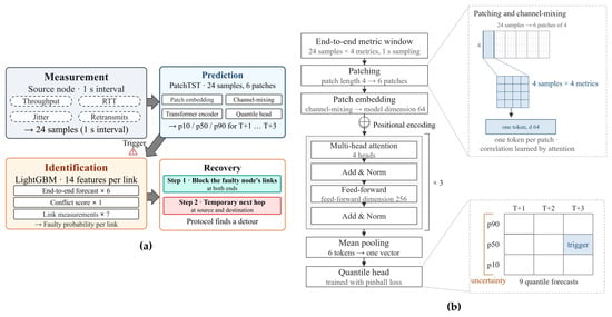
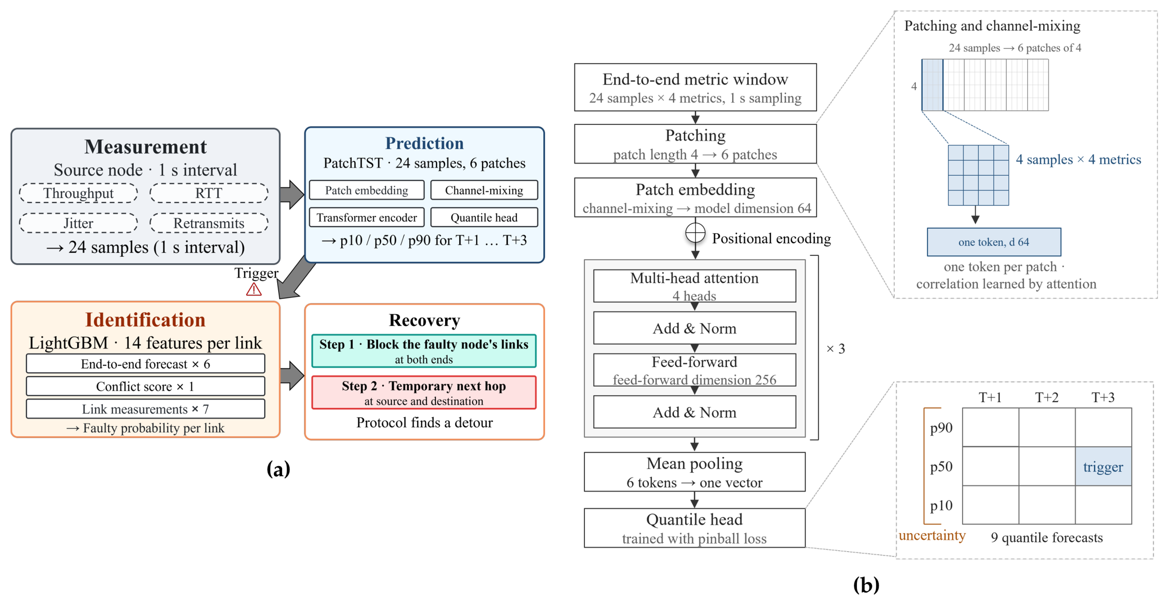
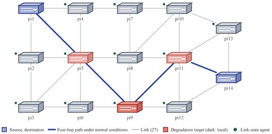
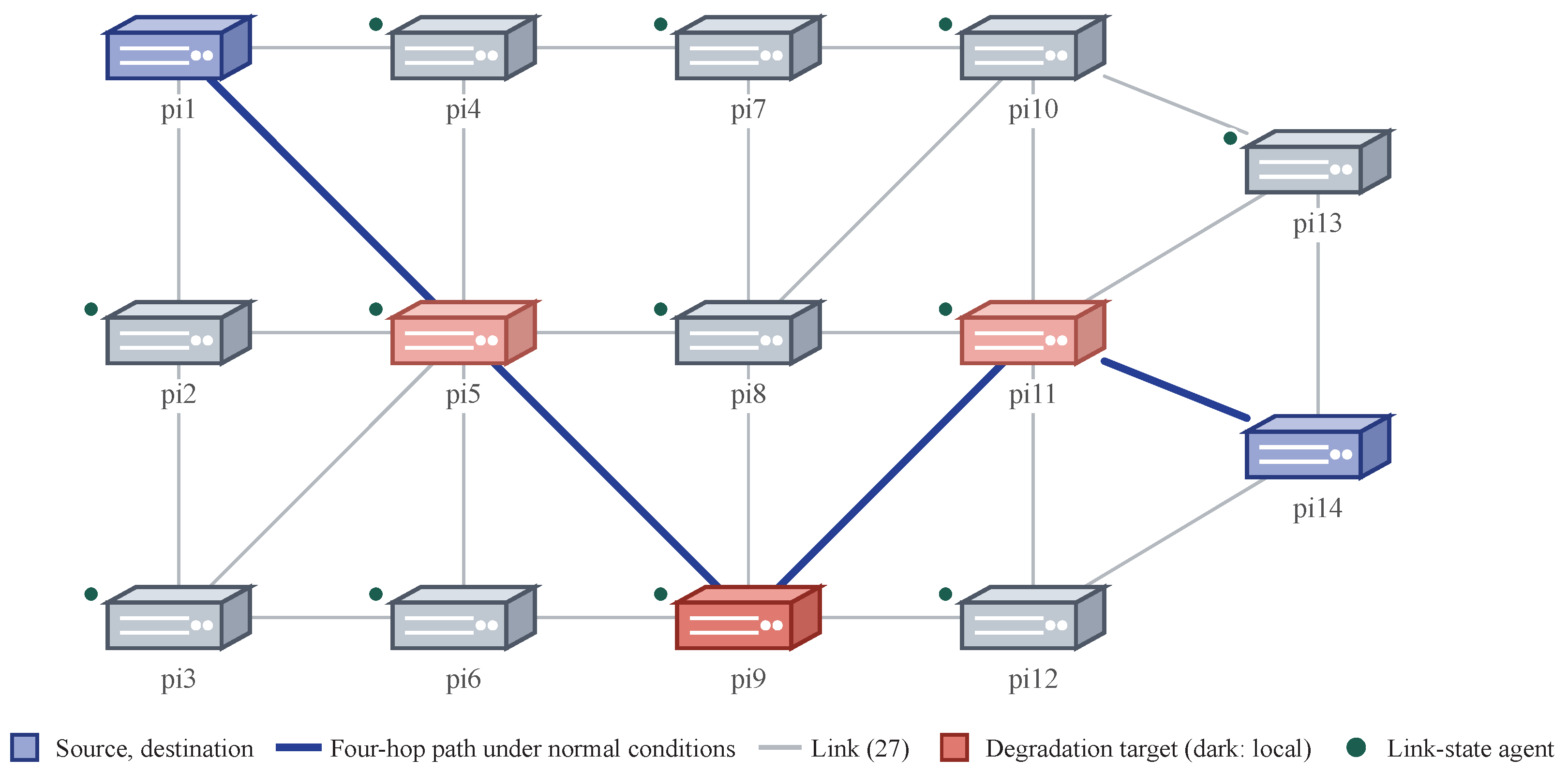
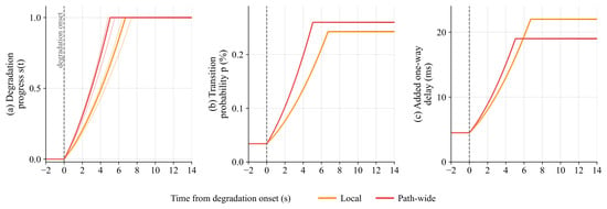
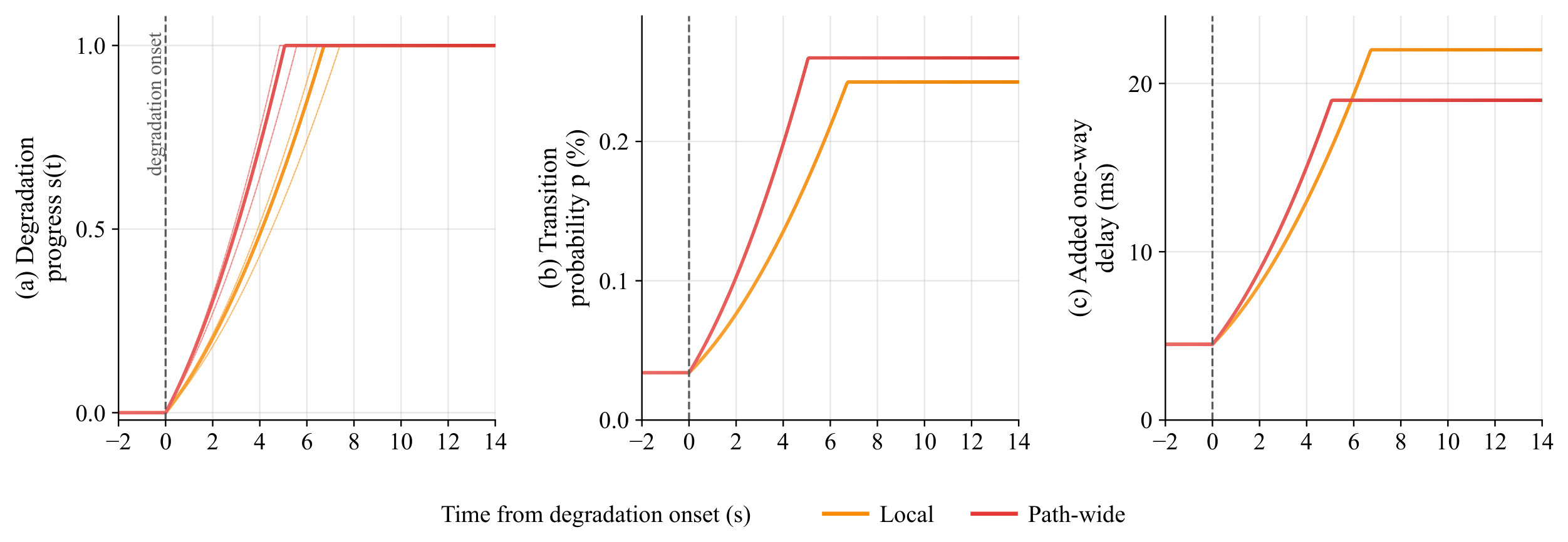
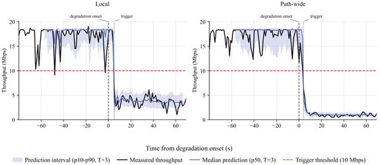
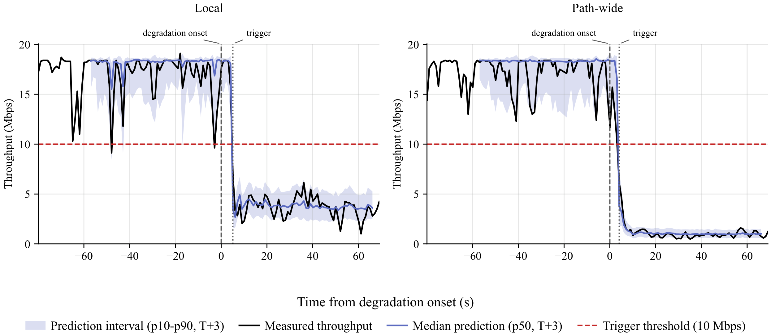
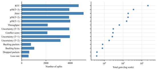
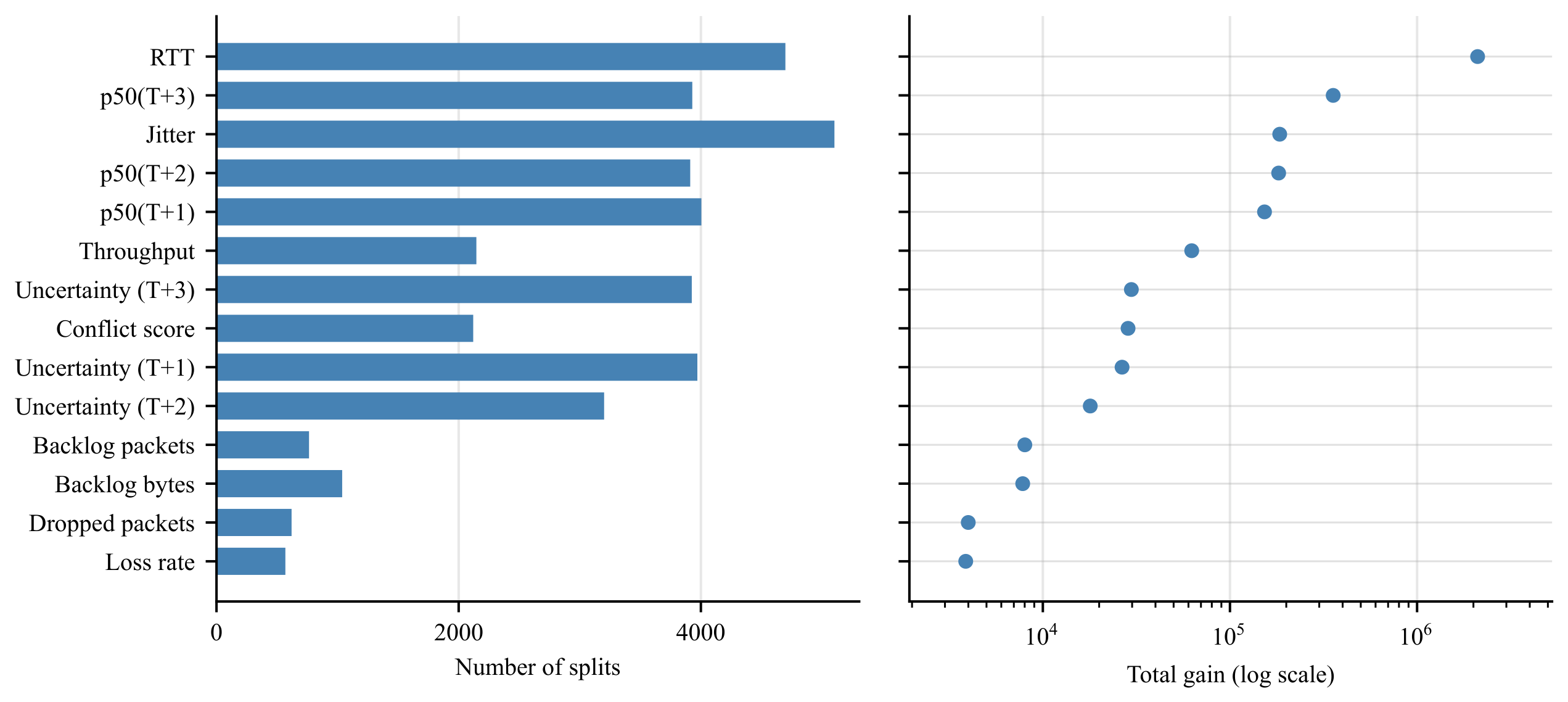
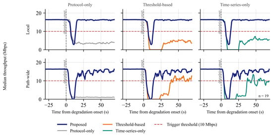
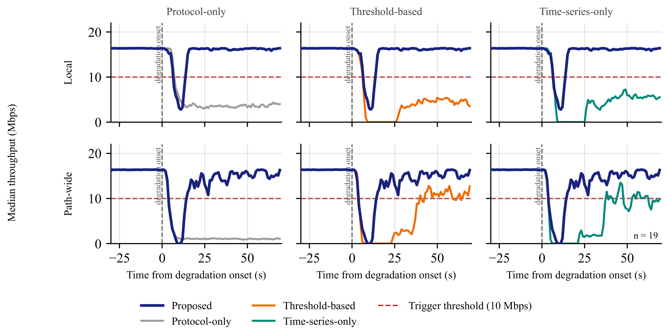
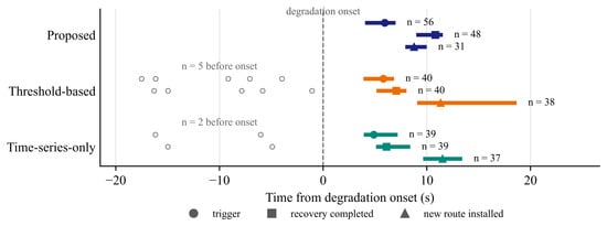
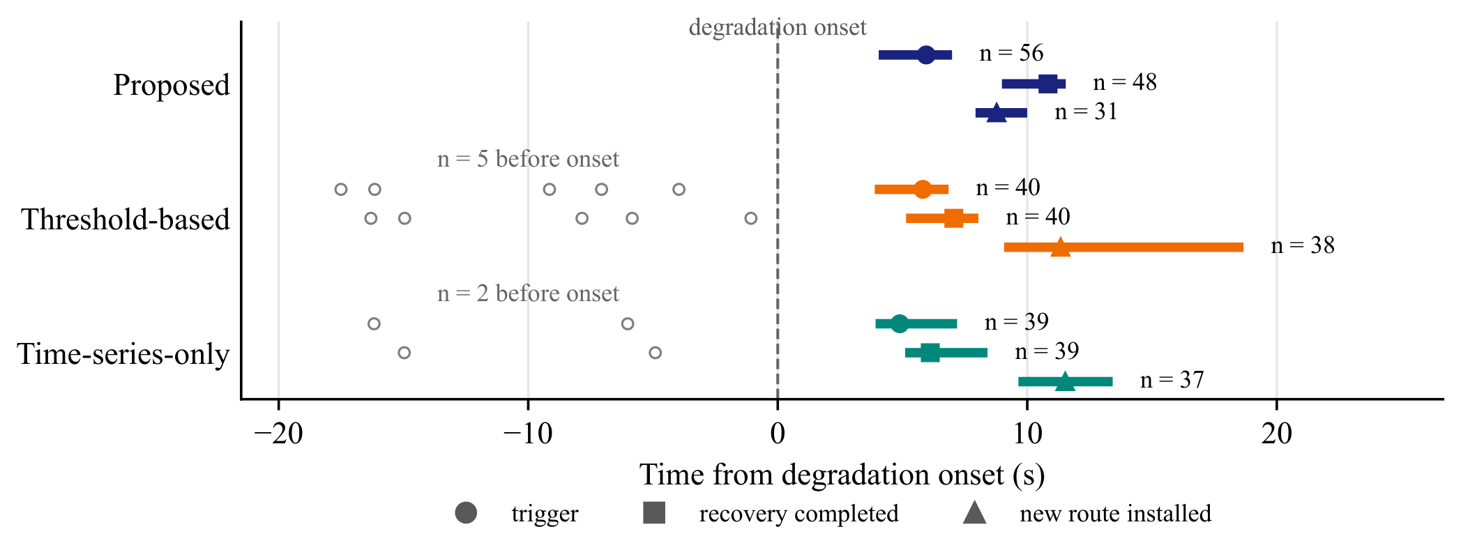

Disclaimer/Publisher’s Note: The statements, opinions and data contained in all publications are solely those of the individual author(s) and contributor(s) and not of MDPI and/or the editor(s). MDPI and/or the editor(s) disclaim responsibility for any injury to people or property resulting from any ideas, methods, instructions or products referred to in the content. |
© 2026 by the authors. Licensee MDPI, Basel, Switzerland. This article is an open access article distributed under the terms and conditions of the Creative Commons Attribution (CC BY) license.