


Abstract
Regional development changes built surfaces, nighttime activity and vegetation, making their spatial correspondence important for land monitoring. Regional averages can obscure whether these changes occur together locally. This exploratory study examined that correspondence in Qinghai using annual satellite observations, climate, terrain and historical management footprints. Observed and partially pooled trajectories characterised 2017–2023 development on a 5 km grid; direct climate-adjusted fixed-effects models and geographically cross-fitted anomalies evaluated vegetation associations, while historical exposure comparisons described protected and mining landscapes. Regional built cover and nighttime light increased, yet observed local co-growth occupied 17.5% of active cells and 39.6% of strong-signal cells. The primary same-year built–NDVI association was approximately 0.0006 NDVI units per fixed reference increment at zero activity change, close to its conditional statistical detection threshold; its ecological importance remains unestablished. Alternative built transformations retained positive estimates, while lead-adjusted fits showed sensitivity to temporal specification. Sanjiangyuan’s positive NDVI-anomaly contrast accompanied prior divergence and raw-NDVI, EVI-anomaly and light intervals spanning zero, leaving its hypothesised outcome combination inconclusive. Muli combined greening with declining light in retained mining cells that were greener and less disturbed than excluded cells. These findings locate regional growth within concentrated local development and distinguish vegetation–activity patterns across managed landscapes, providing a spatial basis for targeted land-use and restoration field checks.
1. Introduction
Land conversion, infrastructure use and vegetation change jointly shape the environmental consequences of development [1,2,3]. Satellite observations capture different parts of this relationship: built cover records classified constructed surfaces, whereas nighttime radiance records emitted light from settlements, infrastructure and production [4,5,6]. Nighttime light provides information about economic activity, with its interpretation depending on electrification, production structure and lighting practices [7,8,9]. Changes in lighting technology can further alter radiance independently of land conversion [10]. The normalised difference vegetation index (NDVI) and enhanced vegetation index (EVI) measure spectral properties of vegetation canopies [11,12]. Their variation integrates climate, atmospheric conditions, disturbance and land management [13,14,15]. Regional growth in construction and light can therefore coexist with different local vegetation trajectories, including greening in established settlements and browning at expansion margins [3,16]. To what extent does regional growth in built cover and nighttime light coincide spatially and temporally with local vegetation change?
Answering this question requires separating aggregate growth from change observed at individual locations. Construction can precede occupancy, and activity can intensify within an existing built footprint, producing asynchronous land and light trajectories [3,17,18]. Decoupling theory provides a vocabulary for such differences, although category assignments depend on the indicator pair, baseline and observation interval [19,20,21]. Endpoint ratios compress the intervening trajectory and become unstable when the denominator changes little [19,21]. Annual observations preserve the direction and timing of change, while sensor calibration and product construction determine which signals are recorded [22,23,24]. Background-masked radiance adds an important distinction between detected activity and recorded nondetection [6,25]. Mixed models can stabilise noisy local trajectories by pooling information across locations [26,27,28]. This pooling makes the distinction between observed and fitted change central to interpretation, as regional mean slopes and local slope signs describe different quantities [26,28]. A joint assessment therefore needs annual trajectories, explicit detection categories and uncertainty at the spatial support of the observations.
Relating those trajectories to vegetation requires an environmental reference because hydrothermal variation can change greenness independently of construction or nighttime activity [13,15,29]. Phenology, vegetation-index design and sensor continuity also affect the temporal signal [12,30,31]. Climate-conditioned analyses compare observed vegetation with an expectation derived from measured environmental conditions [32,33]. Flexible smooths represent nonlinear temperature and water responses, while geographically separated validation tests whether those relationships transfer to new locations [34,35,36]. Such validation is essential when nearby observations share environmental and measurement structure [35,37]. A direct fixed-effects model can estimate vegetation associations with development and climate jointly, holding persistent cell characteristics and common annual conditions constant [38]. Distributed lags describe same-year and lagged associations, while lead terms assess associations with subsequent development change [39]. Geographic-block clustered inference allows correlated residuals within the specified blocks [40]. The ecological question is whether the direction and magnitude of the development–greenness association persist across these environmental references and observational supports.
Protected and restored landscapes provide a further setting in which vegetation and nighttime activity may follow different paths. Conservation outcomes depend on baseline conditions, management and the location of intervention, while environmental and socioeconomic changes can proceed through different mechanisms [41,42,43]. Protected areas are often selected in places with distinctive elevation, accessibility and development pressure, making their comparison populations an explicit part of the estimand [44,45]. Propensity-based designs summarise observed differences, and overlap weights focus the comparison on covariate profiles shared by the exposure groups [46,47,48]. Event-study coefficients display the trajectory before and after a specified management milestone [49,50]. The meaning of that milestone also depends on earlier protection, disturbance and restoration histories, because continuing programmes may affect both exposed and comparison landscapes [41,45]. Separating outcome-specific trajectories consequently serves both environmental monitoring and the design of subsequent impact evaluation [51,52]. These comparisons ask whether greening is accompanied by increasing nighttime activity or instead follows a different trajectory within the managed landscape.
We examine this spatial correspondence in an exploratory study of Qinghai, China, by linking annual built cover, nighttime radiance and vegetation with climate, terrain and documented conservation and mining footprints. Observed trends on a 5 km equal-area grid establish where regional built–light growth is supported by local change during 2017–2023. Active-signal cells provide the primary local development sample, with full and strong-signal domains showing how the result changes with observation support. Direct climate-adjusted fixed-effects models provide the primary vegetation comparison, with geographically cross-fitted anomalies supplying a complementary environmental reference on matched cells and years. Historical Sanjiangyuan and Muli footprints extend the comparison to protected and mining landscapes, using separate outcomes and explicit event-time references. Together, these analyses compare regional growth with observed local co-growth, assess the built–greenness association under alternative climate controls, and describe vegetation–light combinations in historically managed landscapes.
2. Materials and Methods
2.1. Study Area
Qinghai combines a densely settled eastern valley, resource-oriented settlements in the arid Qaidam Basin and extensive sparsely settled alpine landscapes, allowing regional growth to be compared with local signals across contrasting development and hydrothermal conditions. Located at approximately 89.4–103.0° E and 31.6–39.3° N, the province covers about 696,600 km2 and extends from the Qaidam Basin to wetter eastern and southeastern mountains [53]. Population, built land and nighttime activity concentrate in the Yellow River–Huangshui River Valley, while resource extraction creates localised activity elsewhere [54,55]. The extensive historical Sanjiangyuan pilot and the localised Muli mining footprint add contrasting managed landscapes to this environmental gradient. The provincial mask follows the 2019 geoBoundaries gbOpen China ADM1 unit [56]. Development and Sanjiangyuan analyses use 5 km equal-area cells in EPSG:6933; Muli uses 500 m cells in UTM Zone 47N to retain the geometry of mapped mining features (Figure 1).
Figure 1.
Study area and spatial comparison designs. (a) Qinghai within China. (b) Complete-panel Sanjiangyuan treated cells and the 25–100 km comparison ring, with Muli located separately. The Muli inset shows 500 m treated cells, the 2–15 km comparison ring, and map-interpreted mining features. (c) Grid universes and initial policy-comparison counts before support trimming. Colours encode analytical membership. The environmental gradient is shown in Figure S6. Basemap © Mapbox (Washington, DC, USA) © OpenStreetMap.
2.2. Data Sources and Data Processing
2.2.1. Data Sources
The development panel covers 2017–2023, when annual built cover, nighttime radiance and vegetation observations share an observation window. MODIS and climate records beginning in 2010 establish the environmental baselines. Historical boundaries define the landscape comparisons, and populations provide baseline demographic context. Table 1 lists the measurement, validation and exposure-definition roles of each product. Supplementary Section S7 records software, data lineage and the local reproducibility package; Table S12 documents annual radiance encoding.
Table 1.
Data sources and analytical roles.
The annual 10 m land-cover product (version 2) was produced by Impact Observatory (Washington, DC, USA), Microsoft Corporation (Redmond, WA, USA) and Esri (Redlands, CA, USA). Product identifiers and collection versions are reported in Table 1.
2.2.2. Data Processing
Data preprocessing and geospatial analysis used Python version 3.15.2, GDAL version 3.13.3, QGIS version 4.2.3 and ArcGIS Desktop (ArcMap) version 10.8.2 (Esri, Redlands, CA, USA).
Categorical products were summarised by valid class area; radiance and vegetation indices used valid-pixel overlap weights. Missing values remained missing. Joined panels were checked for duplicate cell–year keys, coordinate alignment, units and variable ranges. The provincial grid branches into purpose-specific samples for development trajectories, paired-period maps, ecological regressions and historical comparisons (Table 2; detailed counts in Table S1). These branches overlap and have different completeness rules. Annual climate summaries retained mean temperature and accumulated precipitation on their native 0.5° observational support. Multiple 5 km or 500 m analysis cells therefore share climate information.
Table 2.
Sample flow across purpose-specific analytical branches.
Masked mean VIIRS radiance represents emitted nighttime light. A recorded zero denotes product-level nondetection after background masking; missing values retain a separate status [25]. Radiance in nW cm−2 sr−1 was decoded as (stored value × GDAL band scale + band offset)/10. The activity variable is
Band scales change from 1 in 2017–2021 to 10 in 2022–2023, with zero offsets. The provider distinguishes the EOG-source years 2012–2024 from back-extrapolated 2000–2011 [57]. Development uses 2017–2023, and fitted Sanjiangyuan light records begin in 2012. Table S12 documents supplied-COG decoding checks; Supplementary Section S7 adds the 2017–2021 window and seam diagnostics. The local Chinese Academy of Sciences series supplies common-year rank and direction comparisons.
Built cover was derived from class 7 of the 10 m annual Impact Observatory–Microsoft–Esri product. The built fraction is classified Built area divided by valid classified land area; nodata, water (class 1) and cloud (class 10) are excluded from the denominator. Each annual product aggregates classifications from available Sentinel-2 scenes [72]. For 2017, interpretation distinguishes valid classified land from the availability and seasonal distribution of the underlying observations. The Earth Engine Sentinel-2 surface-reflectance archive documents incomplete global coverage in 2017–2018 [73]; that archive warning concerns a different delivery system from the downloaded IO annual maps. The archived IO inputs contain annual classes rather than per-pixel source-scene histories. ESA WorldCover supplies common-year level comparisons for 2020 and 2021. For the original anomaly regression, removing raw 2017 observations before constructing differences and lags restricts estimation to 2020–2023 (Section 2.3.2; Table S15). The transformed built variable is
which retains recorded zeros. The buffered development domain comprises cells with positive built cover or radiance in any year of 2017–2023 plus a 10 km buffer. Active cells record either signal at least once; strong cells have maximum built fraction above 0.001 or maximum radiance above 0.5. These are retrospective, union-based detection rules. Both-signal detection is tabulated separately. Observed active-cell trajectories are the primary local result; the full and strong domains describe dependence on detection intensity.
May–September Terra MOD13A1 composites were screened before overlap-weighted cell means, and annual medians were calculated. The initial screen used reliability and MODLAND QA classes 0/1 and valid index ranges; annual values require five valid dates. The strict alternative retains reliability 0, MODLAND QA 0, usefulness codes 0/1/2 and aerosol codes 0–2 (excluding high aerosol), and excludes adjacent cloud, mixed cloud, possible snow/ice and shadow flags. It requires 50% valid area per date, with 25%/75% area sensitivities (Supplementary Section S7; [74]). The annual outcomes consistently use Terra; Aqua MYD13A1 offers an eight-day-phased complementary sampling schedule [75]. Combining the two would change the seasonal observation distribution and annual medians, so the present comparison holds the sensor series fixed while varying its quality screen. Development baselines use 2010–2016 medians. CPC maximum/minimum temperatures give daily mean temperature; May–September means/totals represent current temperature/precipitation and October–April represents antecedent conditions. Elevation and slope come from the DEM.
WorldPop provides modelled counts redistributed to approximately 1 km pixels, using settlement and environmental predictors that include nighttime light and land cover. Counts from the China Global 2000–2020 aggregated products for 2010, 2015 and 2020 were summed using fractional pixel–cell overlap after masking negative nodata. Baseline covariates use log(1 + count). Population is demographic context and a weighting covariate; the three-epoch comparison is retained in Supplementary Section S5.1 as a modelled-surface diagnostic, separate from the main outcome evidence [66].
Sanjiangyuan exposure uses the historical 2015–2016 pilot boundary. Exposed 5 km cells have centroids inside and ≥0.80 boundary overlap; primary comparisons lie 25–100 km outside with exposure ≤ 0.20 and pass the Qilian/restoration exclusion envelope. Three alternative rings test geographic support (Supplementary Section S5). The 2016 pilot marks a governance change within an existing protection history, rather than first conservation [76,77]. A separate environmental reference uses 2010–2015 arithmetic-mean baselines and complete provincial pre-pilot observations, with five held-out folds of 50 km blocks. Its training population and validation differ from the development reference (Supplementary Section S3; Table S16).
Muli exposure derives from pits, spoil grounds, coal yards and mine buildings in the published 2020 interpreted map [70]. A six-parameter affine fit to nine graticule intersections gives an internal RMSE of 25.8 m (Supplementary Section S7). Exposed 500 m cells have feature fraction ≥ 0.10. Comparisons lie 2–15 km away, with mapped coverage ≥ 0.80, feature fraction < 0.01 and total mapped human-activity-class fraction ≤ 0.05. Supplementary Section S5 lists the classes, alternative covariates and rings. The 2021–2023 window is compared with 2020 following a 2016–2020 reference window that includes earlier remediation.
Table 2 follows each analytical branch from its starting grid to its retained sample. Sanjiangyuan’s complete 2010–2023 NDVI/EVI rule removes 67 provincial cells: 14 future exposed, one primary-ring comparison and 52 other cells. Propensity trimming subsequently removes 20 exposed and 372 comparison cells from the eligible pool. Muli’s 3819 complete mapped cells contain 216 exposed and 2866 eligible primary comparisons before score trimming. Table S1 provides cell–year totals, and Supplementary Section S7 records the strict-QA sample changes.
2.3. Analytical Models
Three retrospective hypotheses organise this exploratory monitoring study. H1 expects regional built–light growth alongside more locally flat than jointly increasing trajectories. H2 expects a positive same-year built–greenness coefficient at zero nighttime-activity change under alternative climate controls. H3 expects positive vegetation contrasts alongside stable or declining nighttime activity in the historical comparisons. Each outcome is evaluated on its own scale using its estimate and interval. These hypotheses, the active-signal emphasis and sensitivity checks were formulated during revision after inspection of the original results. H1 and H3 describe directional patterns; H2 is assessed by native-index magnitudes and conditional statistical detection thresholds. Ecological importance requires separate vegetation composition or biomass evidence. Figure S4 summarises the analytical sequence.
Statistical analyses were performed in R version 4.5.0 (R Foundation for Statistical Computing, Vienna, Austria). The archived corrected-model sessions used nlme version 3.1-168, mgcv version 1.9-3, data.table version 1.17.8 and Matrix version 1.7-3. The first-revision direct-model fits used data.table version 1.17.8, mgcv version 1.9-3, jsonlite version 2.0.0, digest version 0.6.37 and splines version 4.5.0. Stage-specific software records are described in Supplementary Section S7.4.
2.3.1. Observed and Partially Pooled Built and Light Trajectories
Observed within-cell annual slopes and geographic-block intervals provide the primary trajectory summaries. Active-signal cells contribute the main local comparison; the buffered full domain describes regional context, and the strong-signal domain tests dependence on detection intensity. A correlated mixed model provides a complementary partially pooled trajectory for the active and strong domains [27,28]. Its two outcomes are transformed nighttime radiance and built cover, and time is centred at 2020:
Outcome-specific year deviations, λt, absorb nonlinear shocks common to all cells and are constrained to be orthogonal to the linear trend. Random intercepts, ui, and random slopes, bi, link the two outcomes; their covariance structure and estimation are given in Supplementary Section S2. The empirical-Bayes cell slope is si = β + bi.
Regional mean slopes are evaluated by resampling intact geographic blocks. Local summaries distinguish positive, negative and numerically flat observed slopes, with the latter defined by an absolute slope at most 10−12. These are observed direction counts. Active- and strong-domain empirical-Bayes directions show how pooling changes the same-cell summary. The buffered all-cell fit is retained as a diagnostic of pooling over recorded zeros in Figure S3 and Table S11, alongside the variance-parameter diagnostics in Table S4. Full resampling and covariance details are in Supplementary Section S2.
2.3.2. Vegetation Associations Under Alternative Climate Controls
The primary ecological model regresses observed annual NDVI directly on development changes, current and antecedent climate departures, and cell/year effects, estimating climate and development coefficients jointly in the target sample. A complementary geographic cross-fitting analysis constructs an environmental reference. Its reference cells satisfy five criteria: maximum 2017–2023 built fraction ≤ 0.001, maximum decoded radiance ≤ 0.5 nW cm−2 sr−1, minimum vegetation-valid fraction ≥ 0.50, baseline median NDVI in [0.05, 0.80], and baseline NDVI interquartile range ≤ 0.20. Baselines use 2010–2016. Approximately 100 km geographic blocks are allocated intact to five folds (seed 20260826), with every observation in a held-out block excluded from training. A penalised Gaussian identity-link GAM predicts annual greenness departures using four current/antecedent climate departures, baseline growing-season temperature and precipitation, baseline NDVI, elevation and slope. Three tensor interactions combine current temperature with precipitation, temperature with elevation, and precipitation with elevation [34,35]. This reference is
The complementary climate-conditioned anomaly is
The four climate-departure smooths and elevation use basis dimension 6; baseline terms and slope use dimension 5, and each tensor interaction has 5 × 5 margins. Fitting uses mgcv::bam with fast restricted maximum likelihood, selection penalties and discrete computation, weighted by vegetation-valid share clipped to [0.05, 1]. Positive anomalies indicate greener observations than predicted from the measured climate and terrain covariates. Prediction R2, RMSE, observed-minus-predicted bias and calibration of observed departures on predictions are evaluated separately inside and outside the reference domain. The direct NDVI model and the anomaly model use identical development terms and matched cells within each signal domain.
Annual changes in transformed built cover and activity enter at the current and previous year, together with their within-lag products [39]. The primary direct model is Equation (6): G denotes observed annual NDVI; the four climate departures are growing-season temperature and precipitation and antecedent temperature and precipitation; q contains the original-screen vegetation-valid fraction—the smaller of the NDVI and EVI valid-composite fractions relative to the available annual dates—and an annual radiance-outlier indicator. The latter flags radiance above the provincial within-year 99.9th percentile. The built-valid fraction enters complete-case screening and is removed at the rank check because its within-transformed variation is unidentifiable. The matched strict-QA comparisons retain these original quality controls; strict calendar-date coverage determines their sample eligibility. The anomaly alternative replaces G with Equation (5)’s residual and omits the jointly fitted climate terms. The two models use matched observations and identical development terms, but differ in their outcome construction and climate adjustment.
The active primary panel contains 41,792 cell–years, 8361 cells and 94 spatial blocks during 2019–2023. Its five-year window supports contemporaneous and one-year-lag comparisons. Cell/year effects absorb persistent local and common annual differences. Linear and spline climate controls, anomaly outcomes and elevation-band trends generate six matched-sample specifications per domain, repeated in full and strong domains (Table S19). Spatial CR1 intervals use a normal reference; BH q values adjust six development terms and three cumulative contrasts within each model. Strict-QA comparisons use identical retained cells and years (Table S23). Supplementary Section S7 provides knots and sample rules; Supplementary Sections S4 and S7 retain the original EVI, lead, cell-trend and spatial-influence diagnostics. The baseline-year sensitivity removes raw 2017 observations before constructing differences and lags; the 2018 difference then becomes unavailable, removing the lagged predictor needed for 2019. The original anomaly sensitivity consequently uses 2020–2023, and its lead version uses 2020–2022, with the climatic reference held fixed (Table S15).
Two additional checks target the primary active-cell direct model. The transformation check replaces asinh(100F) with asinh(F), where F is the built fraction, and rebuilds current and lagged differences and their activity interactions on identical 2019–2023 observations. The temporal check adds next-year changes in built cover, activity and their product, using 2019–2022 observations with an observed subsequent year. Models with and without leads are compared on that same reduced sample, both with and without elevation-band trends. Table S24 reports scale sensitivity; Table S25 reports individual and joint lead tests. Supplementary Section S8 specifies sampling, uncertainty and multiplicity adjustment.
2.3.3. Protected and Mining Landscape Comparisons
Overlap weighting concentrates the comparison on covariate profiles represented in both exposure groups, while an event study separates pre-period trajectories from subsequent outcome changes [48,50]. Let Di indicate treatment and e(Xi) = P(Di = 1∣Xi) be the propensity score estimated from baseline ecological, climate, terrain, population, and nighttime-light covariates. The overlap weight is
normalised by the pooled mean weight. Sanjiangyuan uses 13 standardised covariate main effects: 2010–2015 NDVI and EVI means and slopes; log(1 + 2015 population); the 2010–2015 difference in log(1 + population), divided by five; 2012–2015 asinh-radiance mean and slope; log(1 + distance in km to the nearest 2015 settlement proxy); elevation; terrain slope; and 2010–2015 mean growing-season temperature and precipitation. Settlement proxies have population density ≥ 10 persons/km2. Muli’s full 16-term model uses 2016–2020 NDVI, EVI and activity means and slopes, elevation, slope, log(1 + 2015 population), alpine-meadow, bare-land and bare-rock fractions, and 2016–2020 means of growing-season and antecedent temperature and precipitation. Its ecology design removes activity and population; its lean design retains the vegetation, terrain and climate terms. Propensities use intercept-plus-main-effects binomial-logit models on standardised complete cases, fitted before support trimming and carried forward without refitting. Balance is evaluated on retained samples and both fitted transformations and additional diagnostic variables (Supplementary Section S5). The weighted event study is
where Sanjiangyuan event time is indexed to the 2016 pilot, with 2015 as the omitted reference year. Outcomes are climate-adjusted NDVI or EVI, raw NDVI, sensor-validity share and nighttime activity. Equal averaging of the post-milestone coefficients gives the reported exposure contrast. Sanjiangyuan uses 50 km spatial clusters and 999 wild cluster-score draws. Alternative rings and source zones, a false 2013 date, a boundary shifted 250 km east, and sensor validity provide design-specific comparisons. The modelled-population analysis is reported separately in Supplementary Section S5.1.
Muli uses 2020 as reference, 2021–2023 as response, 500 m cells and 2 km blocks. Its event regression adds the linearly independent standardised columns for current and antecedent temperature and precipitation departures to Equation (8). Outcomes are NDVI, EVI, nighttime light and valid-composite share. A separate spatial-translation statistic compares departures from each cell’s pre-response NDVI trend across mapped and translated footprints, retaining field shape and area weights in 999 sampled placement pairs (Supplementary Section S5).
For each Muli covariate design, retained exposed cells are compared with excluded exposed cells from the same 216-cell starting population. Unweighted summaries describe baseline vegetation and light during 2016–2020, terrain, 2015 modelled population and the interpreted July 2020 land-cover and mining classes. Table 6 summarises the comparison, and Table S26 reports means and standard deviations. This population description is separate from exposed–comparison covariate balance after weighting.
Each application estimates descriptive, overlap-weighted trajectory contrasts for a mapped exposure cohort relative to its stated reference year. Pre-period coefficients, covariate balance, comparison rings and sensor-quality outcomes characterise the comparison population [48,50].
Direct-model intervals condition on the observed panel and spatial covariance partition. Original anomaly-model score resampling additionally fixes climate predictions; landscape resampling fixes weights and supplied outcomes. The score procedures quantify uncertainty conditional on these fitted inputs. Development main coefficients are conditional on zero change in the interacting signal. Cross-domain magnitudes use the same 0.074635 SD of built change residualised by cell/year effects in the original full sample. Supplementary Section S7 defines the conditional, single-test 80%-power detection threshold.
3. Results
3.1. Regional Built and Light Growth Was Concentrated in a Subset of Cells
Built cover and nighttime activity increased across the paired-period maps, while vegetation change extended across a much wider part of the province (Figure 2). Among 28,427 cells observed in both windows, mean built cover rose from 0.29% in 2017–2019 to 0.35% in 2021–2023. Mean asinh activity increased from 0.0158 to 0.0226, and mean NDVI from 0.305 to 0.308. Built and activity medians were zero in both periods. In the later period, 82.2% of cells had zero classified built cover and 89.8% had masked radiance equal to zero (Table S2). Thus, positive provincial means summarise development concentrated within a subset of cells.
Figure 2.
Built cover (%), annual asinh nighttime activity and NDVI in 2017–2019 and 2021–2023. The 28,427-cell sample has six complete annual observations for each of four mapped variables, including the climate-conditioned NDVI anomaly. Insets enlarge the outlined Huangshui valley vicinity (101.10–103.00° E, 36.20–36.95° N); the point marks Xining. Insets retain the parent map’s 5 km cells and colour scale. Built/light scales use symmetric-log normalisation, and NDVI uses a linear scale; scales are shared within columns. Grey denotes incomplete pairs. Initial vegetation QA and Albers equal-area projection are used; strict-QA comparisons are reported in Supplementary Section S7.
Observed annual trends supported aggregate co-growth across nested development domains (Figure 3; Table 3). The provincial panel contained 200,459 cell–years across 28,637 cells. Within the 26,543-cell buffered development domain, 26,378 cells supplied at least four finite paired years. Mean within-cell slopes were 0.0018 asinh activity units per year and 0.0037 asinh built-percentage units per year. Their geographic-block bootstrap 95% intervals were 0.0011–0.0028 and 0.0016–0.0064. Both mean slopes remained positive in the active and strong domains, reaching 0.0128 asinh activity units per year and 0.0297 asinh built-percentage units per year among 3339 strong-signal cells (Table S14). Figure 3 shows annual means on the fixed 26,372-cell support with all seven paired years; Table S12 records the radiance encoding and source-to-panel verification.
Figure 3.
Observed annual trajectories and geographic-block trend stability. (a,b) Equal-cell annual means over the 26,372 trajectory-domain cells with seven paired years. (c,d) Mean within-cell ordinary least-squares slopes across full, active, and strong signal domains, with percentile intervals from 9999 resamples of intact 100 km geographic blocks (seed 20260906). The resampling target is the mean observed slope. Table 3 reports the corresponding signal supports, and Figure S3 contrasts observed and empirical-Bayes sign composition.
Table 3.
Observation-supported development trajectories in nested signal domains.
Observed local co-growth increased with signal intensity: both slopes were positive in 17.5% of active cells and 39.6% of strong-signal cells, compared with 5.6% of the buffered full domain. The respective shares with at least one numerically flat slope were 73.3%, 44.1% and 91.5% (Table 3). Among cells with both signals detected at least once, the corresponding observed co-growth shares were 64.6% in the active domain and 70.2% in the strong domain (Table S11). Of the 26,378 full-domain cells, 18,016 (68.3%) recorded neither signal in any year, and 2268 recorded both signals at least once. Pooling changed the local classification substantially: the full-domain empirical-Bayes co-growth share was 90.3%, including all 18,016 neither-signal cells; the strong-domain share was 71.5% (Figure S3; Table S11). Independent light comparisons gave common-positive rank correlations of 0.864–0.880 and annual direction agreement of 0.727–0.814. Built-cover rank correlations with WorldCover were 0.543 and 0.551 for 2020 and 2021 (Table S4).
The positive regional trend also appeared before the 2021/2022 encoding change. On fixed seven-year-complete membership, active-domain 2017–2021 slopes were 0.0587 built-cover percentage points and 0.0051 asinh light units per year; corresponding 2017–2023 slopes were 0.0499 and 0.0057. With asinh built percentage, local co-growth was 13.8% versus 17.5%. Three-year median smoothing of built percentage gave 17.3% active-cell co-growth over seven years. At 10 km, area-aggregated active and strong domains gave 20.4% and 53.7% co-growth, compared with 17.4% and 39.4% using raw built percentage at 5 km. The 2021/2022 active-cell light increment was 0.0056 below the mean of the four preceding increments (block-bootstrap 95% CI −0.0092 to −0.0023). These results preserve the early-window growth direction while showing that grain and the annual seam affect local summaries (Figure S5; Table S20).
3.2. Development and Vegetation Change Occupied Different Spatial Supports
Development and vegetation changes had different spatial footprints (Figure 4). The mean paired changes were +0.061 percentage points in built cover, +0.0068 in asinh activity, +0.0034 in NDVI and +0.0027 in the climate-conditioned NDVI anomaly. Built and activity changes were exactly zero in 74.7% and 88.8% of paired cells, whereas the central 80% of NDVI changes ranged from −0.019 to +0.026. Below 3000 m, mean built and activity increases were 0.30 percentage points and 0.025 asinh units. At 4000–5000 m, the corresponding built increase was 0.0017 percentage points, and the mean anomaly increase was 0.007 (Tables S2 and S3). Figure S2 shows the full distributions across the three signal domains.
Figure 4.
Paired changes in built cover (percentage points), asinh nighttime activity, NDVI and climate-conditioned NDVI anomaly: 2021–2023 minus 2017–2019 means on 28,427 complete cells. Insets enlarge the outlined Huangshui valley vicinity (101.10–103.00° E, 36.20–36.95° N), preserving the 5 km cells and parent-panel colour scale; the point marks Xining. Symmetric limits use the provincial 98th percentile of absolute change with a fixed floor; triangles mark saturated tails. Blue/orange show decreases/increases; grey denotes incomplete pairs. Initial vegetation QA and Albers equal-area projection are used; strict-QA comparisons are reported separately.
Pooled held-out NDVI R2 was 0.226 for 165,018 reference observations and 0.063 for 35,334 non-reference observations (Figure 5; Table 4). Corresponding RMSE values were 0.023 and 0.034; calibration slopes were 0.889 and 0.678. All five fits converged, with training R2 of 0.266–0.285. EVI held-out R2 values were 0.242 and 0.190, with RMSE values of 0.017 and 0.020, respectively. These metrics evaluate the geographic climate reference used to construct the anomalies.
Figure 5.
Pooled geographic cross-fitting performance for NDVI and EVI. Stable reference landscapes and non-reference transfer landscapes are evaluated separately. (a) Out-of-sample R2. (b) Root mean squared error. (c) Mean prediction bias. (d) Calibration slope. Bias and RMSE retain each index’s native units. Dashed lines: bias = 0 and calibration slope = 1. Each index has 165,018 reference and 35,334 non-reference held-out observations; all geographic folds are pooled.
Table 4.
Geographic cross-fitting performance by prediction domain.
The active-signal direct model relates annual NDVI levels positively to same-year built change, with a coefficient of 0.0076 (95% CI 0.0025–0.0126; nine-term q = 0.029; Figure 6). On the common residualised-built-change scale, this corresponds to 0.00057 NDVI units (0.00019–0.00094), conditional on zero activity change. The conditional 80%-power detection threshold on the same scale is 0.00054 NDVI. The model uses 41,792 observations from 8361 cells and 94 spatial blocks during 2019–2023. The corresponding anomaly-model coefficient is 0.0079 (0.0016–0.0141; q = 0.119). Both models yield positive same-year built–greenness estimates on the matched active sample.
Figure 6.
Same-year built–greenness coefficients under matched-sample climate controls. Panels show the active primary, full and strong domains, with six specifications in each. Points and bars are coefficients and normal-reference 95% spatial-cluster intervals; the q column reports within-model nine-term Benjamini–Hochberg adjustment. Coefficients are NDVI or NDVI-anomaly units per unit change in asinh (100 × built fraction), conditional on zero activity change. Direct models use observed NDVI and jointly fitted climate terms; anomaly models use the fixed geographic reference. Samples are identical within each domain. Table S19 gives the common-scale magnitudes, detectable effects and complete specification details.
All 18 same-year built estimates were positive, with differing precision (Table S19). In active cells, adding elevation-band trends reduced the direct linear coefficient to 0.0058 (0.0018–0.0099; q = 0.043); spline controls gave 0.0063 without trends and 0.005 with trends (q = 0.032 and 0.052). All three strong-domain trend-adjusted intervals spanned zero.
The original full-domain anomaly coefficient was 0.0094, equivalent to 7 × 10⁻⁴ NDVI-anomaly units on the common scale, and its within-transformed R2 was 0.0022. Its EVI alternative was 0.0037 (−0.00006 to 0.0074; q = 0.268). The original full-domain cell-trend built lead was −0.0095 (−0.0148 to −0.0042; q = 0.0013). Three blocks supplied 68.9% of that model’s same-year built-coefficient variance; deleting them reduced the estimate to 0.0059 (0.0012–0.0106; q = 0.124). Supplementary Sections S4 and S7 and Tables S5, S6 and S17–S19 retain these original-model diagnostics separately from the primary active-cell tests below.
The strict-QA comparison retained 32,590 observations from 7225 active cells and 93 blocks, after excluding 8818 observations failing annual strict coverage and 384 fixed-effect singleton observations (Table S23). On that identical sample, changing the NDVI screen reduced the same-year built coefficient from 0.0099 to 0.0093; with elevation-band trends, it changed from 0.0084 to 0.0080 (strict 95% CI 0.0037–0.0123; q = 0.002). The latter corresponds to 0.0006 NDVI on the common change scale. Strict-QA activity intervals spanned zero, and cumulative associations varied with trend adjustment. Accepted composite starts also shifted; in 2020 and 2021 the strict common sample averaged about nine days later than the initial screen. These comparisons separate the effects of outcome screening, sample selection and seasonal coverage on the estimated association.
Replacing asinh(100F) with asinh(F) on the same 41,792 observations gave a same-year built coefficient of 0.222 (95% CI 0.074–0.371; q = 0.030), compared with 0.0076 (0.0025–0.0126; q = 0.029) under the primary transformation. With elevation-band trends, the alternative coefficient was 0.149 (0.021–0.277; q = 0.068), compared with 0.0058 (0.0018–0.0099; q = 0.043). The coefficients use their respective transformed units: both signs remained positive, while trend-adjusted precision depended on scale (Table S24).
The primary-model lead check used 33,430 observations from 8359 active cells and 94 blocks during 2019–2022. With all three next-year terms included, the built lead was −0.0028 (95% CI −0.0089 to 0.0034; p = 0.379), and the joint lead-test p value was 0.325. On these same observations, the same-year built coefficient changed from 0.0054 (0.0008–0.0099) without leads to 0.0038 (−0.0029 to 0.0105) with leads. Adding elevation-band trends gave a built lead of −0.0054 (−0.0108 to 0.00007; p = 0.053; joint p = 0.062) and a same-year estimate of approximately zero (−0.0059 to 0.0058). These fits locate the temporal sensitivity within the primary active-cell model (Table S25).
3.3. Protected and Mining Landscapes Had Distinct Outcome Trajectories
The Sanjiangyuan primary comparison retains 4674 exposed and 6641 comparison cells, with 158,410 environmental cell–years and 173 clusters (Table S1). Its separate pre-pilot climate reference has held-out NDVI R2 of 0.375 and 0.384 in those groups, with RMSE values of 0.016 and 0.018, respectively (Table S16). The 2016–2023 NDVI-anomaly contrast is 0.0044 (95% CI 0.00019–0.0086; wild p = 0.035). Raw NDVI and EVI-anomaly contrasts are 0.003 (−0.0021 to 0.0081) and 0.0011 (−0.0016 to 0.0038). The 2012–2023 light series gives a subsequent-period contrast of −0.00029 (−0.0008 to 0.00022). Figure 7 and Table 5 retain these distinct outcome scales; the dependent three-epoch modelled-population result is reported in Supplementary Section S5.1.
Figure 7.
Sanjiangyuan exposure trajectories and design diagnostics. (a) NDVI-anomaly event coefficients relative to 2015. (b) Outcome-specific subsequent-period contrasts, displayed on separate scales: NDVI units for the NDVI-anomaly and raw-NDVI rows, EVI units for the EVI-anomaly row, and asinh radiance units for nighttime activity. Coefficients are shown without numerical rescaling. (c) Alternative comparison rings and source zones on the NDVI-anomaly scale. (d) Remaining covariate imbalance, including the distinction between raw and fitted log settlement distance. Bars are normal-reference spatial-cluster 95% intervals. The primary anomaly contrast is 0.0044, with wild p = 0.035 and joint pre-period p = 0.019. Sensor-validity p = 0.036. The design describes retained exposure groups; intervals condition on fitted weights and supplied outcome surfaces.
Table 5.
Outcome-specific historical exposure contrasts.
NDVI-anomaly contrasts ranged from 0.0030 to 0.0047 across comparison rings; the Yangtze-source estimate was 0.00009 and the Yellow–Lancang estimate 0.0107. The primary joint pre-period test indicated prior divergence (p = 0.019; Table S22), and maximum raw-covariate SMD was 0.293. Sensor validity differed by 0.0333 percentage points (95% CI 0.0030–0.0635; wild p = 0.036). False-date and shifted-boundary p values were 0.373 and 0.850. Prior divergence, the sensor-validity contrast and the raw-NDVI, EVI-anomaly and light intervals spanning zero leave H3 inconclusive for Sanjiangyuan (Figure S1; Table S7).
Muli showed positive vegetation contrasts accompanied by a negative nighttime-light estimate (Figure 8). The full-covariate design retained 208 cells and 64 blocks, including 36 treated cells in 18 treated-side blocks, and yielded an NDVI contrast of 0.0451 (95% CI: 0.0185–0.0717; wild p = 0.002). Ecology and lean designs retained 253 and 435 cells and gave NDVI contrasts of 0.0472 and 0.0447. The lean design supplies a common multi-outcome comparison: its EVI contrast was 0.0361, activity contrast −0.102, and sensor-validity contrast −0.0037 (Table 5). The observed map covers 3819 local cells, while adjusted estimates refer to their separately retained samples. Treated-side block counts were 18, 23, and 32 in the full, ecology, and lean designs (Table S13).
Figure 8.
Muli vegetation contrasts, outcome patterns and spatial diagnostics. (a) NDVI differences for three covariate designs and three alternative comparison rings; the lean comparison design uses 2–15 km. (b) Observed cell-level NDVI difference between the 2021–2023 mean and the 2016–2020 mean, with interpreted mining features outlined. All annual observations in both windows are required; this descriptive change differs from the adjusted event-study contrast. Other outcome estimates are tabulated in Table 5. (c) The field-shape greenness statistic compared with 999 translations. The statistic is the mean 2021–2023 departure from each cell’s 2016–2020 linear trend minus the clean-control mean; it is a different estimand from the weighted event-study coefficients. (d) Maximum post-weighting covariate imbalance, full-design treated-cell retention and lean-design pretrend diagnostic. Error bars show conventional spatial-block 95% confidence intervals. Exposure follows the published interpreted mining footprint, and the comparison describes its vegetation and light trajectories across the 2020 response milestone. The spatial translation p-value evaluates spatial unusualness under the specified translation design. Full covariate results are shown in Figure S1. The translation reference comprises draws from 12 eligible JHG placements and 201 eligible JC placements, with fieldwise shape preserved. Treated-side block counts and group-specific weight ESS are reported in Table S13.
Muli’s field-shape statistic was 0.121, compared with 0.0337 on average across 999 sampled non-overlapping placement pairs (p = 0.001). The finite reference contains 12 eligible JHG placements and 201 eligible JC placements. Maximum post-weighting SMD was 0.649 in the full design and 0.742 in the lean design; the latter arose from bare-rock cover, an additional diagnostic omitted from the lean propensity model, whose fitted covariates had a maximum SMD of 0.0584. NDVI joint pre-period p values were 0.201, 0.116 and 0.001 for the full, ecology and lean samples. Lean activity and valid-date tests had p = 0.002 and 0.001. The results describe mapped-footprint trajectories within their respective retained samples (Tables S8–S10).
Support trimming retained 36, 46 and 97 of the 216 exposed Muli cells in the full, ecology and lean designs, respectively. Relative to excluded cells, all three retained populations had higher baseline NDVI, more alpine meadow, gentler terrain and smaller mapped mining-target fractions (Table 6). In the full design, mean baseline NDVI was 0.389 versus 0.276, meadow cover was 66.2% versus 20.1%, and mining-target cover was 21.7% versus 47.8%. All 36 retained full-design cells had zero recorded baseline light. The three designs therefore describe selected, greener portions of the mapped mining landscape, with distinct retained memberships (Table S26).
Table 6.
Characteristics of retained and excluded exposed Muli cells.
Regional growth and local co-growth have different spatial footprints: jointly increasing observed built and light trajectories occur in a minority of active cells, while vegetation change extends beyond development concentrations. This observed pattern supports H1’s regional–local distinction. The primary built–NDVI association lies close to the conditional statistical detection threshold. Its positive sign persists under the alternative transformation, while lead adjustment changes its precision and trend-adjusted estimate, making H2 dependent on temporal specification. H3 remains inconclusive in Sanjiangyuan. Muli exhibits greening with declining light in a retained subset characterised by greater meadow cover and less mapped disturbance. Together, these findings identify where the signals coincide and which comparison populations they describe. Table 7 connects each finding to its diagnostics and interpretation.
Table 7.
Findings, diagnostics and interpretation.
4. Discussion
4.1. Regional Co-Growth and Local Change Have Different Spatial Footprints
Regional development concentrated in a much smaller set of locations than a provincial growth average suggests. Both built cover and light increased in the regional mean, while observed co-growth occupied 17.5% of active cells and 39.6% of strong-signal cells. This contrast connects the annual trend to the locations supplying its signal. Earlier land–light studies identified asynchronous construction and lighting during infrastructural transition [3,18]. Here, the detection categories show how sparse observations shape the geography of that comparison.
The observed-versus-pooled comparison reveals a specific consequence of applying a continuous mixed model to a landscape with many recorded zeros. Partial pooling moves weak cell slopes toward the population trajectory [26,27]. In the buffered full-domain fit, it assigned positive slopes for both outcomes to every one of the 18,016 cells with neither signal detected. Those classifications express the fitted population trend rather than local observed growth. Using observed slopes for the primary local result and restricting the principal mixed-model comparison to active cells keeps regional estimation distinct from local detection. The full-domain fit returned a non-positive-definiteness diagnostic for its approximate variance-parameter covariance, distinct from the fitted random-effect covariance (Table S4). Table S11 gives the observed–pooled cross-tabulation.
Built cover and radiance record different observable processes: construction changes classified surface cover, while occupancy, production and lighting practice influence emitted light [5,6,17]. Positive regional slopes also occurred during 2017–2021, before the encoding-scale transition. At 5 km, transformation and three-year median smoothing produced similar co-growth shares, whereas aggregation to 10 km increased the share, especially in strong-signal cells (Figure S5). The 10 km comparison changes both the signals aggregated within each cell and the cells meeting the detection thresholds. WorldCover supplies two-year-level agreement, and cell-series smoothing tests temporal sensitivity. Validation of annual conversion requires independently interpreted changed pixels. Parcel conversion and image-quality records would distinguish land change from annual classification fluctuations. Huang et al. [78] identify terrain-related classification difficulties and the value of plateau-specific vegetation classes in a 2022 land-cover map. This evidence provides context for interpreting the IO inputs; the common-year WorldCover comparisons and the original anomaly model’s baseline-year sensitivity assess separate aspects of measurement reliability.
4.2. Vegetation Change Differed from the Spatial Concentration of Development
Vegetation change was distributed beyond the main development concentrations. The largest built and light increases occurred below 3000 m, whereas the 4000–5000 m group showed a larger mean climate-conditioned greenness increase. Greening and browning also coexisted within the positive provincial mean. Hydrothermal conditions, vegetation composition and disturbance can produce this spatial variation [15,29]. The elevation summaries place the largest development increases and climate-conditioned greenness increases in different elevation bands.
The initial climatic reference predicted annual NDVI departures with held-out RMSE values of 0.023 in reference and 0.034 in non-reference landscapes; corresponding EVI errors were 0.017 and 0.020. Geographic validation therefore measures transfer to the target environments [35,36]. Sanjiangyuan’s separately trained pre-pilot model has its own validation in Table S16.
Sensor validation addresses a different measurement scale: NASA’s approximately ±0.025 NDVI accuracy statement concerns high-quality near-nadir 16-day Collection-6 observations, rather than this study’s Collection-6.1 annual aggregates [79]. Aggregation can reduce random error, while correlated bias and selective seasonal coverage can persist. The direct model and strict-QA checks test complementary parts of this measurement chain. A clustered-SE detection threshold quantifies statistical sensitivity; vegetation composition or biomass observations would be needed to assign ecological importance to a 0.00057-NDVI contrast. At high elevation, May snow persistence and September snowfall can reduce snow-free coverage or shift the dates represented in an annual median. Detailed snow/cloud screening and valid-area thresholds address flagged observations, while the retained composite-start dates describe the accompanying seasonal selection [74].
The direct-model comparison locates the vegetation association on its native scale and shows its dependence on temporal specification. In active cells, the common-scale difference was 0.00057 NDVI, close to the conditional detection threshold of 0.00054, declining to 0.00044 after elevation-band trends and 0.00038 with spline controls and trends. Strong-domain trend-adjusted intervals span zero. Refitting asinh(F) retained positive same-year estimates on identical observations, with precision depending on trend adjustment. Adding one-year leads to the primary direct model yielded a negative built lead with an interval spanning zero and a same-year estimate whose interval also spanned zero; with elevation-band trends, the same-year point estimate was approximately zero (Tables S24 and S25). Thus, the spatial association is more clearly described than its temporal ordering. At 5 km, construction and vegetation change can occur in different parts of the same cell, consistent with studies separating established urban areas from expansion margins [16,80]. Shared evolving conditions and annual measurement covariance provide additional explanations for the coincident changes. The mapped correspondence therefore identifies locations for joint land-conversion and vegetation observations, with ecological importance to be established through composition or biomass measurements.
4.3. Landscape History Explains the Role of the Exposure Comparisons
Sanjiangyuan’s NDVI-anomaly contrast is positive, while the raw NDVI, EVI-anomaly and light intervals span zero. Prior divergence (joint p = 0.019) and a sensor-validity contrast (p = 0.036) make the hypothesised vegetation–activity combination inconclusive in this comparison. Its conservation history also predates the 2016 pilot: the ecological protection programme began in 2005, and Phase II was launched in 2014 [76,81]. Regional studies connect vegetation change to grazing pressure, climate and successive engineering stages [82,83]. The pilot comparison describes trajectories within this continuing conservation landscape. Cell-level histories of programme coverage and implementation intensity would connect the observed differences to successive management stages.
Muli paired positive vegetation contrasts with lower nighttime light in the overlap-supported mining populations. The retained cells had higher baseline NDVI, more alpine meadow and smaller mining-target fractions than the excluded exposed cells; the full design additionally retained cells with zero baseline recorded light (Table 6). These contrasts characterise the greener, less disturbed portion of the mapped footprint. Restrictions and remediation were documented from 2014, alongside later evidence of incomplete enforcement and illegal extraction [84,85]. Long-term vegetation records also place recent greening within an extended mining history [86]. Disturbance cessation, natural recovery and active rehabilitation are plausible contributors, while production and lighting records would help interpret the radiance decline. The translation result locates unusually large detrended greenness at the mapped footprint relative to its finite placement reference. Mine-specific implementation and closure records would distinguish the processes contributing to that spatial pattern.
Prior trajectories and baseline differences define the interpretation of the exposure contrasts. Sanjiangyuan’s joint pre-period p = 0.019 and Muli lean NDVI/light p = 0.001/0.002 place the later differences within already divergent landscapes. Raw settlement-distance SMD remains 0.293 after balancing its fitted log transformation. Muli’s full maximum SMD is 0.649; lean fitted terms reach 0.0584, while omitted bare-rock cover reaches 0.742. The intervals quantify conditional sampling uncertainty; prior selection, trajectory differences and support trimming define the populations being compared. Table 7 synthesises these descriptive, outcome-specific findings in relation to their management histories.
4.4. Multi-Signal Monitoring Targets Places for Field Verification
A land manager in the Huangshui valley could use the zoomed maps to select active 5 km cells where built cover increased but nighttime activity remained flat, then inspect the observed annual series to distinguish a persistent pattern from an isolated annual jump. Parcel permits, recent imagery and occupancy records would help determine whether a flagged cell contains new construction awaiting use or an annual classification change. Overlaying the raw and climate-conditioned vegetation maps would then prioritise locations for a vegetation check, with strict-QA coverage informing the survey season. At Muli, the corresponding screen would identify greening and declining light within the retained mining population described in Table 6, followed by checks of closure records, restoration dates and plant composition. The output is a shortlist of locations and questions for verification. The regional NDVI association supplies context for that screening, while field observations establish the condition of each selected parcel.
Modelled population supplies demographic context through covariates that share information with satellite settlement and activity products. Direct census, household and implementation observations would test the social and management processes underlying the mapped trajectories [51,52]. The practical output is a spatially explicit comparison of complementary signals, with locations, scales and outcome definitions preserved for subsequent investigation.
5. Conclusions
Regional growth statistics summarise development, while local trajectories reveal its environmental geography. This exploratory study examined how regional built-cover and nighttime-light growth relates to local vegetation change, connecting aggregate trends with heterogeneous landscape conditions.
Annual satellite observations, climate, terrain and historical management footprints were integrated in Qinghai. Observed trajectories described local built–light change, direct climate-adjusted models evaluated vegetation associations, and historical comparisons characterised protected and mining landscapes at their respective spatial and temporal supports.
Regional built cover and nighttime activity increased, while observed local co-growth occupied 17.5% of active cells and 39.6% of strong-signal cells. At zero activity change, the primary direct model estimated 0.00057 NDVI units per common built-change increment (95% CI 0.00019–0.00094), close to the conditional 80%-power detection threshold of 0.00054. Its ecological importance remains unestablished without composition or biomass observations. Alternative built transformations retained positive point estimates, while lead adjustment made the same-year intervals span zero; all strong-domain trend-adjusted intervals also spanned zero. Sanjiangyuan’s prior divergence, sensor-validity contrast and outcome intervals leave H3 inconclusive. Muli combined higher vegetation indices with lower light in the greener, less disturbed retained mining population. The findings connect regional growth to concentrated local development and show how observation support and landscape history shape vegetation–activity comparisons.
The available data provide annual satellite observations, 0.5° climate inputs and mapped management footprints. Independent validation of annual built-cover transitions, a cell-level inventory of earlier conservation programmes, higher-resolution climate inputs and census-based population comparisons remain outside the present evidence base. These additions would refine land-change accuracy, environmental adjustment and management histories. Vegetation composition, biomass, occupancy and dated restoration records would connect the satellite contrasts to ecological and land-use processes.
The central implication is that regional growth and local environmental change should be monitored together at explicitly stated spatial supports. Separating observed local trajectories from regional means and keeping vegetation and nighttime activity as distinct outcomes can guide field checks and targeted follow-up studies. This correspondence provides a concrete basis for interpreting heterogeneous development and restoration landscapes.
Supplementary Materials
The following supporting information can be downloaded at: https://www.mdpi.com/article/10.3390/app162110977/s1, Supplementary Sections S1–S9, Figures S1–S6 and Tables S1–S25 and S26a–c. Figure S1. Absolute standardized covariate differences before and after overlap weighting. Figure S2. Empirical cumulative distributions of paired-period change within the full trajectory, active-signal and strong-signal domains. Figure S3. Observed and empirical-Bayes direction composition in the same cells. Figure S4. Data-to-analysis workflow and observation supports. Figure S5. Observation-based sensitivity to time window, transformation and spatial grain. Figure S6. Environmental gradient across the Qinghai analysis grid. Table S1. Analysis supports and time windows. Table S2. Complete paired-period distributions. Table S3. Changes across elevation bands. Table S4. Trajectory diagnostics and independent product comparisons. Table S5. Original anomaly-model coefficient families. Table S6. Original anomaly-model lead diagnostics. Table S7. Sanjiangyuan comparison and diagnostic record. Table S8. Muli propensity support, balance, and spatial dependence units. Table S9. Muli joint pre-period tests by outcome and covariate design. Table S10. Muli ring and field-specific contrasts. Table S11. Signal support and observed-versus-pooled co-growth. Table S12. Annual radiance encoding and lineage verification. Table S13. Muli treated-side and comparison-side dependence support. Table S14. Observed-slope and conditional mixed-model uncertainty. Table S15. Original anomaly-model samples and time support. Table S16. Held-out pre-policy validation of the Sanjiangyuan climate reference. Table S17. Same-year built association after influential-block deletion. Table S18. Spatial covariance partitions for the fixed same-year built estimate. Table S19. Same-year built coefficients across all matched-sample specifications. Table S20. Selected observation-based sensitivity summaries. Table S21. Strict-QA NDVI availability and composite-start timing. Table S22. Sanjiangyuan primary pre-period event coefficients. Table S23. Direct NDVI comparisons on identical strict-QA-supported cells and years. Table S24. Transformation sensitivity of the primary same-year built–NDVI association. Table S25. Same-year and future built-change associations in matched active cells. Table S26a. Exposed-cell characteristics for the full design. Table S26b. Exposed-cell characteristics for the ecology design. Table S26c. Exposed-cell characteristics for the lean design.
Author Contributions
Conceptualisation, Y.Y. and L.W.; software, Y.Y.; writing—original draft preparation, Y.W., S.W. and L.W.; visualisation, L.W. All authors have read and agreed to the published version of the manuscript.
Funding
This research was funded by the Science and Technology Project Contract of Qinghai Province under the Science and Technology Development Subsidy Fund “Research on Key Technologies of Urban Physical Examination and Dynamic Optimization Based on Large Artificial Intelligence Models”, grant number 2026-FZ-03.
Institutional Review Board Statement
Not applicable.
Informed Consent Statement
Not applicable.
Data Availability Statement
Source products and access addresses are listed in Table 1 and Supplementary Section S7. The processed analysis data and code form part of ongoing follow-up research; their public release is deferred at this stage.
Conflicts of Interest
Authors Yan Wang and Yan Yang were employed by the company Qinghai Provincial Planning and Design Research Institute Co., Ltd. The remaining authors (Shan Wang and Lei Wang) declare that the research was conducted in the absence of any commercial or financial relationships that could be construed as a potential conflict of interest.
References
- Seto, K.C.; Fragkias, M.; Güneralp, B.; Reilly, M.K. A meta-analysis of global urban land expansion. PLoS ONE 2011, 6, e23777. [Google Scholar] [CrossRef] [Scilit] [PubMed]
- Seto, K.C.; Güneralp, B.; Hutyra, L.R. Global forecasts of urban expansion to 2030 and direct impacts on biodiversity and carbon pools. Proc. Natl. Acad. Sci. USA 2012, 109, 16083–16088. [Google Scholar] [CrossRef] [Scilit] [PubMed]
- Stokes, E.C.; Seto, K.C. Characterizing urban infrastructural transitions for the Sustainable Development Goals using multi-temporal land, population, and nighttime light data. Remote Sens. Environ. 2019, 234, 111430. [Google Scholar] [CrossRef] [Scilit]
- Small, C.; Pozzi, F.; Elvidge, C.D. Spatial analysis of global urban extent from DMSP-OLS night lights. Remote Sens. Environ. 2005, 96, 277–291. [Google Scholar] [CrossRef] [Scilit]
- Elvidge, C.D.; Baugh, K.; Zhizhin, M.; Hsu, F.-C.; Ghosh, T. VIIRS night-time lights. Int. J. Remote Sens. 2017, 38, 5860–5879. [Google Scholar] [CrossRef] [Scilit]
- Levin, N.; Kyba, C.C.M.; Zhang, Q.; Sánchez de Miguel, A.; Román, M.O.; Li, X.; Portnov, B.A.; Molthan, A.L.; Jechow, A.; Miller, S.D.; et al. Remote sensing of night lights: A review and an outlook for the future. Remote Sens. Environ. 2020, 237, 111443. [Google Scholar] [CrossRef] [Scilit]
- Henderson, J.V.; Storeygard, A.; Weil, D.N. Measuring economic growth from outer space. Am. Econ. Rev. 2012, 102, 994–1028. [Google Scholar] [CrossRef] [Scilit] [PubMed]
- Donaldson, D.; Storeygard, A. The view from above: Applications of satellite data in economics. J. Econ. Perspect. 2016, 30, 171–198. [Google Scholar] [CrossRef] [Scilit]
- Mellander, C.; Lobo, J.; Stolarick, K.; Matheson, Z. Night-time light data: A good proxy measure for economic activity? PLoS ONE 2015, 10, e0139779. [Google Scholar] [CrossRef] [Scilit] [PubMed]
- Kyba, C.C.M.; Kuester, T.; Sánchez de Miguel, A.; Baugh, K.; Jechow, A.; Hölker, F.; Bennie, J.; Elvidge, C.D.; Gaston, K.J.; Guanter, L. Artificially lit surface of Earth at night increasing in radiance and extent. Sci. Adv. 2017, 3, e1701528. [Google Scholar] [CrossRef] [Scilit] [PubMed]
- Tucker, C.J. Red and photographic infrared linear combinations for monitoring vegetation. Remote Sens. Environ. 1979, 8, 127–150. [Google Scholar] [CrossRef] [Scilit]
- Huete, A.; Didan, K.; Miura, T.; Rodriguez, E.P.; Gao, X.; Ferreira, L.G. Overview of the radiometric and biophysical performance of the MODIS vegetation indices. Remote Sens. Environ. 2002, 83, 195–213. [Google Scholar] [CrossRef] [Scilit]
- Nemani, R.R.; Keeling, C.D.; Hashimoto, H.; Jolly, W.M.; Piper, S.C.; Tucker, C.J.; Myneni, R.B.; Running, S.W. Climate-driven increases in global terrestrial net primary production from 1982 to 1999. Science 2003, 300, 1560–1563. [Google Scholar] [CrossRef] [Scilit]
- Zhu, Z.; Piao, S.; Myneni, R.B.; Huang, M.; Zeng, Z.; Canadell, J.G.; Ciais, P.; Sitch, S.; Friedlingstein, P.; Arneth, A.; et al. Greening of the Earth and its drivers. Nat. Clim. Change 2016, 6, 791–795. [Google Scholar] [CrossRef] [Scilit]
- Piao, S.; Wang, X.; Park, T.; Chen, C.; Lian, X.; He, Y.; Bjerke, J.W.; Chen, A.; Ciais, P.; Tømmervik, H.; et al. Characteristics, drivers and feedbacks of global greening. Nat. Rev. Earth Environ. 2020, 1, 14–27. [Google Scholar] [CrossRef] [Scilit]
- Zhang, X.; Brandt, M.; Tong, X.; Tong, X.; Zhang, W.; Fensholt, R. Urban core greening balances browning in urban expansion areas in China during recent decades. J. Remote Sens. 2024, 4, 0112. [Google Scholar] [CrossRef] [Scilit]
- Li, Z.; Luan, W.; Zhang, Z.; Su, M. Relationship between urban construction land expansion and population/economic growth in Liaoning Province, China. Land Use Policy 2020, 99, 105022. [Google Scholar] [CrossRef] [Scilit]
- Chen, T.-H.K.; Chen, W.; Stokes, E.C.; Zhou, Y. Detecting gaps between urban expansion and lighting infrastructure growth using daytime and nighttime satellite imagery. Int. J. Appl. Earth Obs. Geoinf. 2026, 146, 105087. [Google Scholar] [CrossRef] [Scilit]
- Tapio, P. Towards a theory of decoupling: Degrees of decoupling in the EU and the case of road traffic in Finland between 1970 and 2001. Transp. Policy 2005, 12, 137–151. [Google Scholar] [CrossRef] [Scilit]
- Ward, J.D.; Sutton, P.C.; Werner, A.D.; Costanza, R.; Mohr, S.H.; Simmons, C.T. Is decoupling GDP growth from environmental impact possible? PLoS ONE 2016, 11, e0164733. [Google Scholar] [CrossRef] [Scilit]
- Wiedenhofer, D.; Virág, D.; Kalt, G.; Plank, B.; Streeck, J.; Pichler, M.; Mayer, A.; Krausmann, F.; Brockway, P.; Schaffartzik, A.; et al. A systematic review of the evidence on decoupling of GDP, resource use and GHG emissions, part I: Bibliometric and conceptual mapping. Environ. Res. Lett. 2020, 15, 063002. [Google Scholar] [CrossRef] [Scilit]
- Zhang, Q.; Seto, K.C. Mapping urbanization dynamics at regional and global scales using multi-temporal DMSP/OLS nighttime light data. Remote Sens. Environ. 2011, 115, 2320–2329. [Google Scholar] [CrossRef] [Scilit]
- Li, X.; Zhou, Y. A stepwise calibration of global DMSP/OLS stable nighttime light data (1992–2013). Remote Sens. 2017, 9, 637. [Google Scholar] [CrossRef] [Scilit]
- Gibson, J.; Olivia, S.; Boe-Gibson, G.; Li, C. Which night lights data should we use in economics, and where? J. Dev. Econ. 2021, 149, 102602. [Google Scholar] [CrossRef] [Scilit]
- Elvidge, C.D.; Zhizhin, M.; Ghosh, T.; Hsu, F.-C.; Taneja, J. Annual time series of global VIIRS nighttime lights derived from monthly averages: 2012 to 2019. Remote Sens. 2021, 13, 922. [Google Scholar] [CrossRef] [Scilit]
- Laird, N.M.; Ware, J.H. Random-effects models for longitudinal data. Biometrics 1982, 38, 963–974. [Google Scholar] [CrossRef] [Scilit]
- Pinheiro, J.C.; Bates, D.M. Mixed-Effects Models in S and S-PLUS; Springer: Berlin/Heidelberg, Germany, 2000. [Google Scholar] [CrossRef] [Scilit]
- Gelman, A.; Hill, J. Data Analysis Using Regression and Multilevel/Hierarchical Models; Cambridge University Press: Cambridge, UK, 2007. [Google Scholar] [CrossRef] [Scilit]
- Pettorelli, N.; Vik, J.O.; Mysterud, A.; Gaillard, J.-M.; Tucker, C.J.; Stenseth, N.C. Using the satellite-derived NDVI to assess ecological responses to environmental change. Trends Ecol. Evol. 2005, 20, 503–510. [Google Scholar] [CrossRef] [Scilit]
- de Jong, R.; de Bruin, S.; de Wit, A.J.W.; Schaepman, M.E.; Dent, D.L. Analysis of monotonic greening and browning trends from global NDVI time-series. Remote Sens. Environ. 2011, 115, 692–702. [Google Scholar] [CrossRef] [Scilit]
- Fensholt, R.; Proud, S.R. Evaluation of Earth Observation based global long term vegetation trends: Comparing GIMMS and MODIS global NDVI time series. Remote Sens. Environ. 2012, 119, 131–147. [Google Scholar] [CrossRef] [Scilit]
- Chen, J.; Yan, F.; Lu, Q. Spatiotemporal variation of vegetation on the Qinghai–Tibet Plateau and the influence of climatic factors and human activities on vegetation trend (2000–2019). Remote Sens. 2020, 12, 3150. [Google Scholar] [CrossRef] [Scilit]
- Yang, D.; Liu, Y. Heterogeneous impacts of human activities and climate change on transformed vegetation dynamics on the Qinghai–Tibet Plateau. J. Environ. Manag. 2025, 392, 126575. [Google Scholar] [CrossRef] [Scilit]
- Wood, S.N. Generalized Additive Models: An Introduction with R, 2nd ed.; Chapman and Hall/CRC: Boca Raton, FL, USA, 2017. [Google Scholar] [CrossRef] [Scilit]
- Roberts, D.R.; Bahn, V.; Ciuti, S.; Boyce, M.S.; Elith, J.; Guillera-Arroita, G.; Hauenstein, S.; Lahoz-Monfort, J.J.; Schröder, B.; Thuiller, W.; et al. Cross-validation strategies for data with temporal, spatial, hierarchical, or phylogenetic structure. Ecography 2017, 40, 913–929. [Google Scholar] [CrossRef] [Scilit]
- Valavi, R.; Elith, J.; Lahoz-Monfort, J.J.; Guillera-Arroita, G. blockCV: An R package for generating spatially or environmentally separated folds for k-fold cross-validation of species distribution models. Methods Ecol. Evol. 2019, 10, 225–232. [Google Scholar] [CrossRef] [Scilit]
- Ploton, P.; Mortier, F.; Réjou-Méchain, M.; Barbier, N.; Picard, N.; Rossi, V.; Dormann, C.; Cornu, G.; Viennois, G.; Bayol, N.; et al. Spatial validation reveals poor predictive performance of large-scale ecological mapping models. Nat. Commun. 2020, 11, 4540. [Google Scholar] [CrossRef] [Scilit] [PubMed]
- Wooldridge, J.M. Econometric Analysis of Cross Section and Panel Data, 2nd ed.; The MIT Press: Cambridge, MA, USA, 2010; ISBN 978-0-262-23258-6. Available online: https://mitpress.mit.edu/9780262232586/econometric-analysis-of-cross-section-and-panel-data/ (accessed on 30 October 2026).
- Gasparrini, A. Modeling exposure–lag–response associations with distributed lag non-linear models. Stat. Med. 2014, 33, 881–899. [Google Scholar] [CrossRef] [Scilit]
- Cameron, A.C.; Miller, D.L. A practitioner’s guide to cluster-robust inference. J. Hum. Resour. 2015, 50, 317–372. [Google Scholar] [CrossRef] [Scilit]
- Ferraro, P.J.; Pattanayak, S.K. Money for nothing? A call for empirical evaluation of biodiversity conservation investments. PLoS Biol. 2006, 4, e105. [Google Scholar] [CrossRef] [Scilit]
- Andam, K.S.; Ferraro, P.J.; Pfaff, A.; Sanchez-Azofeifa, G.A.; Robalino, J.A. Measuring the effectiveness of protected area networks in reducing deforestation. Proc. Natl. Acad. Sci. USA 2008, 105, 16089–16094. [Google Scholar] [CrossRef] [Scilit]
- Ferraro, P.J.; Hanauer, M.M. Quantifying causal mechanisms to determine how protected areas affect poverty through changes in ecosystem services and infrastructure. Proc. Natl. Acad. Sci. USA 2014, 111, 4332–4337. [Google Scholar] [CrossRef] [Scilit]
- Joppa, L.N.; Pfaff, A. High and far: Biases in the location of protected areas. PLoS ONE 2009, 4, e8273. [Google Scholar] [CrossRef] [Scilit]
- Rodrigues, A.S.L.; Cazalis, V. The multifaceted challenge of evaluating protected area effectiveness. Nat. Commun. 2020, 11, 5147. [Google Scholar] [CrossRef] [Scilit]
- Rosenbaum, P.R.; Rubin, D.B. The central role of the propensity score in observational studies for causal effects. Biometrika 1983, 70, 41–55. [Google Scholar] [CrossRef]
- Stuart, E.A. Matching methods for causal inference: A review and a look forward. Stat. Sci. 2010, 25, 1–21. [Google Scholar] [CrossRef] [Scilit]
- Li, F.; Morgan, K.L.; Zaslavsky, A.M. Balancing covariates via propensity score weighting. J. Am. Stat. Assoc. 2018, 113, 390–400. [Google Scholar] [CrossRef] [Scilit]
- Sun, L.; Abraham, S. Estimating dynamic treatment effects in event studies with heterogeneous treatment effects. J. Econom. 2021, 225, 175–199. [Google Scholar] [CrossRef] [Scilit]
- Roth, J.; Sant’Anna, P.H.C.; Bilinski, A.; Poe, J. What’s trending in difference-in-differences? A synthesis of the recent econometrics literature. J. Econom. 2023, 235, 2218–2244. [Google Scholar] [CrossRef] [Scilit]
- Oldekop, J.A.; Holmes, G.; Harris, W.E.; Evans, K.L. A global assessment of the social and conservation outcomes of protected areas. Conserv. Biol. 2016, 30, 133–141. [Google Scholar] [CrossRef] [Scilit] [PubMed]
- Naidoo, R.; Gerkey, D.; Hole, D.; Pfaff, A.; Ellis, A.M.; Golden, C.D.; Herrera, D.; Johnson, K.; Mulligan, M.; Ricketts, T.H.; et al. Evaluating the impacts of protected areas on human well-being across the developing world. Sci. Adv. 2019, 5, eaav3006. [Google Scholar] [CrossRef] [Scilit]
- Qinghai Provincial People’s Government. Geography and Natural Conditions of Qinghai. 2020. Available online: https://www.qinghai.gov.cn/dmqh/system/2020/10/10/010368324.shtml (accessed on 30 October 2026). (In Chinese)
- Wang, Y.; Liu, Z.; He, C.; Xia, P.; Liu, Z.; Liu, H. Quantifying urbanization levels on the Tibetan Plateau with high-resolution nighttime light data. Geogr. Sustain. 2020, 1, 233–244. [Google Scholar] [CrossRef] [Scilit]
- Yin, C.; Zhu, A.L.; Zhou, Q.; Meng, F.; Chen, R.; Liu, F.; Chen, Q.; Guo, X. Rapid urban expansion and potential disaster risk on the Qinghai–Tibetan Plateau in the 21st century. Landsc. Ecol. 2024, 39, 35. [Google Scholar] [CrossRef] [Scilit]
- Runfola, D.; Anderson, A.; Baier, H.; Crittenden, M.; Dowker, E.; Fuhrig, S.; Goodman, S.; Grimsley, G.; Layko, R.; Melville, G.; et al. geoBoundaries: A global database of political administrative boundaries. PLoS ONE 2020, 15, e0231866. [Google Scholar] [CrossRef] [Scilit]
- Hengl, T. Annual Time Series of Global VIIRS Nighttime Lights for 2000–2024 at 500-m Spatial Resolution Extrapolated Using Logistic Regression [Data Set]. Zenodo. 2025. Available online: https://zenodo.org/records/17294744 (accessed on 30 October 2026).
- Impact Observatory; Microsoft; Esri. 10 m Annual Land Use Land Cover (9-Class), Version 2, 2017–2023 [Data Set]. Microsoft Planetary Computer. 2024. Available online: https://planetarycomputer.microsoft.com/dataset/io-lulc-annual-v02 (accessed on 30 October 2026).
- Didan, K. MODIS/Terra Vegetation Indices 16-Day L3 Global 500 m SIN Grid V061 (MOD13A1.061) [Data Set]. NASA LP DAAC. 2021. Available online: https://ladsweb.modaps.eosdis.nasa.gov/missions-and-measurements/products/MOD13A1 (accessed on 30 October 2026).
- NOAA Physical Sciences Laboratory. CPC Global Daily Maximum and Minimum Temperature [Data Set]. Available online: https://psl.noaa.gov/data/gridded/data.cpc.globaltemp.html (accessed on 30 October 2026).
- NOAA Physical Sciences Laboratory. CPC Global Unified Gauge-Based Analysis of Daily Precipitation [Data Set]. Available online: https://psl.noaa.gov/data/gridded/data.cpc.globalprecip.html (accessed on 30 October 2026).
- Chen, M.; Shi, W.; Xie, P.; Silva, V.B.S.; Kousky, V.E.; Higgins, R.W.; Janowiak, J.E. Assessing objective techniques for gauge-based analyses of global daily precipitation. J. Geophys. Res. Atmos. 2008, 113, D04110. [Google Scholar] [CrossRef] [Scilit]
- European Space Agency. Copernicus DEM GLO-30 [Data Set]. Available online: https://dataspace.copernicus.eu/explore-data/data-collections/copernicus-contributing-missions/collections-description/COP-DEM (accessed on 30 October 2026).
- European Space Agency. WorldCover 2020/2021 [Data Set]. Available online: https://esa-worldcover.org/ (accessed on 30 October 2026).
- Chinese Academy of Sciences Resources and Environmental Science Data Center. National Annual Nighttime-Light Dataset, 2013–2021 [Data Set]. Available online: https://www.resdc.cn/ (accessed on 30 October 2026).
- WorldPop; Center for International Earth Science Information Network (CIESIN). Global High Resolution Population Denominators Project [Data Set]. 2018. Available online: https://hub.worldpop.org/ (accessed on 30 October 2026).
- National Tibetan Plateau Data Center. Vector Boundary Dataset of Sanjiangyuan National Park [Dataset]. 2020. Available online: https://data.tpdc.ac.cn/zh-hans/data/a2cc2fb2-ba29-4059-af5f-6d58acf654c8/ (accessed on 30 October 2026). (In Chinese)
- Sanjiangyuan National Park Administration. Sanjiangyuan National Park Master Plan [Official Public Document]. 2018. Available online: https://sjy.qinghai.gov.cn/storage/app/media/uploaded-files/20180309110108_.pdf (accessed on 30 October 2026). (In Chinese)
- National Forestry and Grassland Administration. Qilian Mountain National Park Master Plan [Draft for Public Consultation]. 2019. Available online: https://www.forestry.gov.cn/html/main/main_4461/20190215090310544360608/file/20190215091240236906983.pdf (accessed on 30 October 2026). (In Chinese)
- Wang, H.; Qi, Y.; Zhang, J.; Zhang, J.; Yang, R.; Guo, J.; Luo, D.; Wu, J.; Zhou, S. Influence of open-pit coal mining on ground surface deformation of permafrost in the Muli Region in the Qinghai–Tibet Plateau, China. Remote Sens. 2022, 14, 2352. [Google Scholar] [CrossRef] [Scilit]
- Qinghai Provincial Department of Transport. Muli Mining Area Advances Vegetation Restoration Work. 2020. Available online: https://jtyst.qinghai.gov.cn/jtyst/2020-12/22/article_2022121414543259395.html (accessed on 30 October 2026). (In Chinese)
- Impact Observatory. Methodology & Accuracy Summary: 10m Global Land Use Land Cover Maps. July 2022. Available online: https://www.impactobservatory.com/legal/lulc-methodology-accuracy.pdf (accessed on 30 October 2026).
- Google Earth Engine. Harmonized Sentinel-2 MSI: MultiSpectral Instrument, Level-2A (SR). Earth Engine Data Catalog. Available online: https://developers.google.com/earth-engine/datasets/catalog/COPERNICUS_S2_SR_HARMONIZED (accessed on 10 October 2026).
- Didan, K.; Barreto Munoz, A. MODIS Vegetation Index User’s Guide (MOD13 Series), Version 3.10, Collection 6.1. The University of Arizona. 2019. Available online: https://modis-land.gsfc.nasa.gov/pdf/MOD13_User_Guide_V61.pdf (accessed on 30 October 2026).
- NASA MODIS. MODIS Vegetation Index Products (NDVI and EVI). Available online: https://ladsweb.modaps.eosdis.nasa.gov/missions-and-measurements/science-domain/vegetation-indices (accessed on 10 October 2026).
- Sanjiangyuan Phase-II Plan. Plan for Phase II of Ecological Protection and Construction in Qinghai Sanjiangyuan (Public Version). December 2013; Publicly Hosted by the National Development and Reform Commission. Available online: https://www.ndrc.gov.cn/fzggw/jgsj/njs/sjdt/201404/W020191101564621097541.pdf (accessed on 30 October 2026). (In Chinese)
- National Development and Reform Commission. Progress of the National Park System Pilot I: Sanjiangyuan National Park. 2021. Available online: https://www.ndrc.gov.cn/fzggw/jgsj/shs/sjdt/202104/t20210421_1276872.html (accessed on 30 October 2026). (In Chinese)
- Huang, X.; Yin, Y.; Feng, L.; Tong, X.; Zhang, X.; Li, J.; Tian, F. A 10 m resolution land cover map of the Tibetan Plateau with detailed vegetation types. Earth Syst. Sci. Data 2024, 16, 3307–3332. [Google Scholar] [CrossRef] [Scilit]
- MOD13 Validation Status. Status for: Vegetation Indices (MOD13): General Accuracy Statement. NASA MODIS Land Team. Collection 6 Product Status Updated February 2024. Available online: https://modis-land.gsfc.nasa.gov/ValStatus.php?ProductID=MOD13 (accessed on 8 October 2026).
- Wang, M.; Peng, J.; Hu, Y.; Du, Y.; Qiu, S.; Zhao, M. Scale consistency for investigating urbanization level, vegetation coverage, and their correlation. Urban For. Urban Green. 2021, 59, 126998. [Google Scholar] [CrossRef] [Scilit]
- Sanjiangyuan Ecological Protection. Ecological Protection in Qinghai Sanjiangyuan: A New Historical Advance. Ministry of Finance Official Website. Available online: https://www.mof.gov.cn/zhengwuxinxi/xinwenlianbo/qinghaicaizhengxinxilianbo/201501/t20150116_1180976.htm (accessed on 16 January 2015). (In Chinese)
- Zhang, L.; Fan, J.; Zhou, D.; Zhang, H. Ecological Protection and Restoration Program Reduced Grazing Pressure in the Three-River Headwaters Region, China. Rangel. Ecol. Manag. 2017, 70, 540–548. [Google Scholar] [CrossRef] [Scilit]
- Zhai, X.; Liang, X.; Yan, C.; Xing, X.; Jia, H.; Wei, X.; Feng, K. Vegetation Dynamic Changes and Their Response to Ecological Engineering in the Sanjiangyuan Region of China. Remote Sens. 2020, 12, 4035. [Google Scholar] [CrossRef] [Scilit]
- Li, C.; Wang, T.; Wang, H.; Hu, Z.; Jiang, X.; Liang, Z.; Wang, W.; Du, B. Monitoring technology and method of ecological environment rehabilitation and treatment in Jvhugeng mining area. J. China Coal Soc. 2021, 46, 1451–1462. [Google Scholar] [CrossRef]
- Lan, L. Why Sustained Follow-Through Was Emphasized for the Problems in the Muli Mining Area. China Discipline Inspection and Supervision News. Available online: https://jjjcz.mee.gov.cn/xsjw/202104/t20210412_828238.html (accessed on 12 April 2021). (In Chinese)
- Jiang, L.; Cui, T.; Liu, H.; Xue, Y. Remote Sensing Monitoring and Analytical Evaluation of Grasslands in the Muli Region of Qinghai, China from 2000 to 2021. Land 2022, 11, 1733. [Google Scholar] [CrossRef] [Scilit]
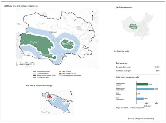
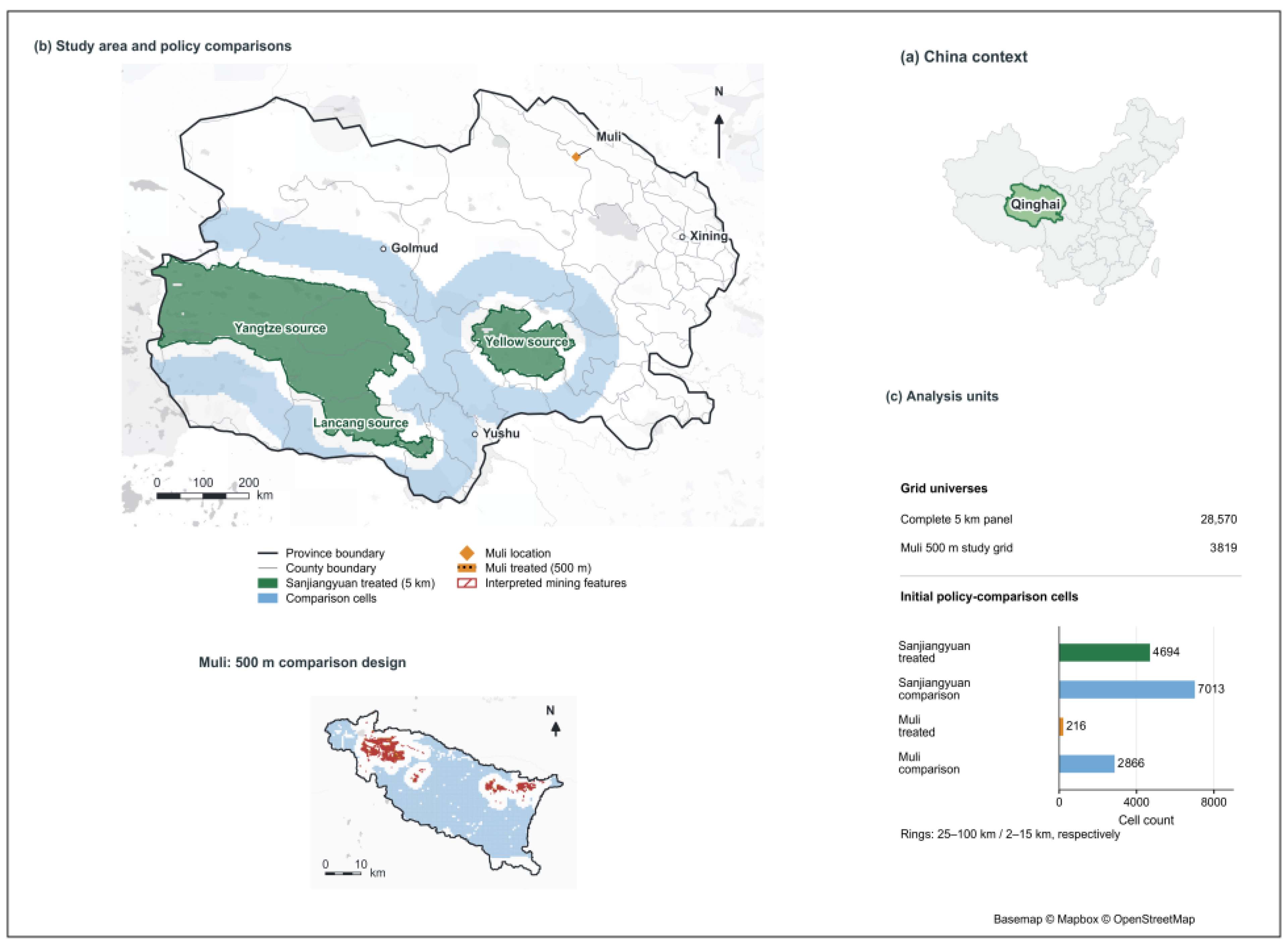
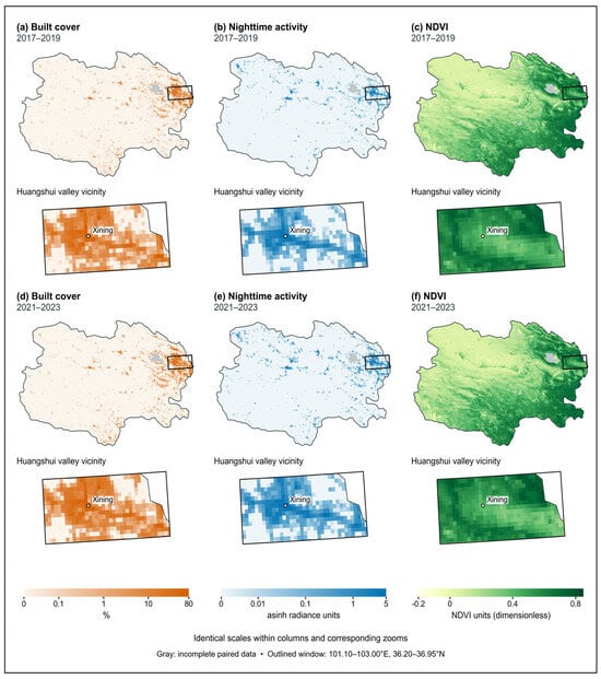
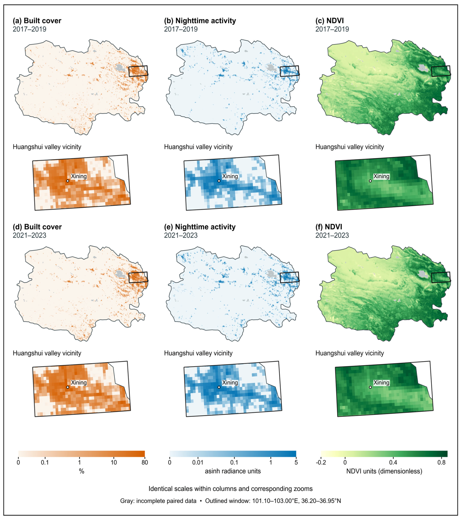
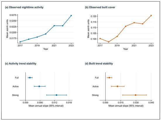
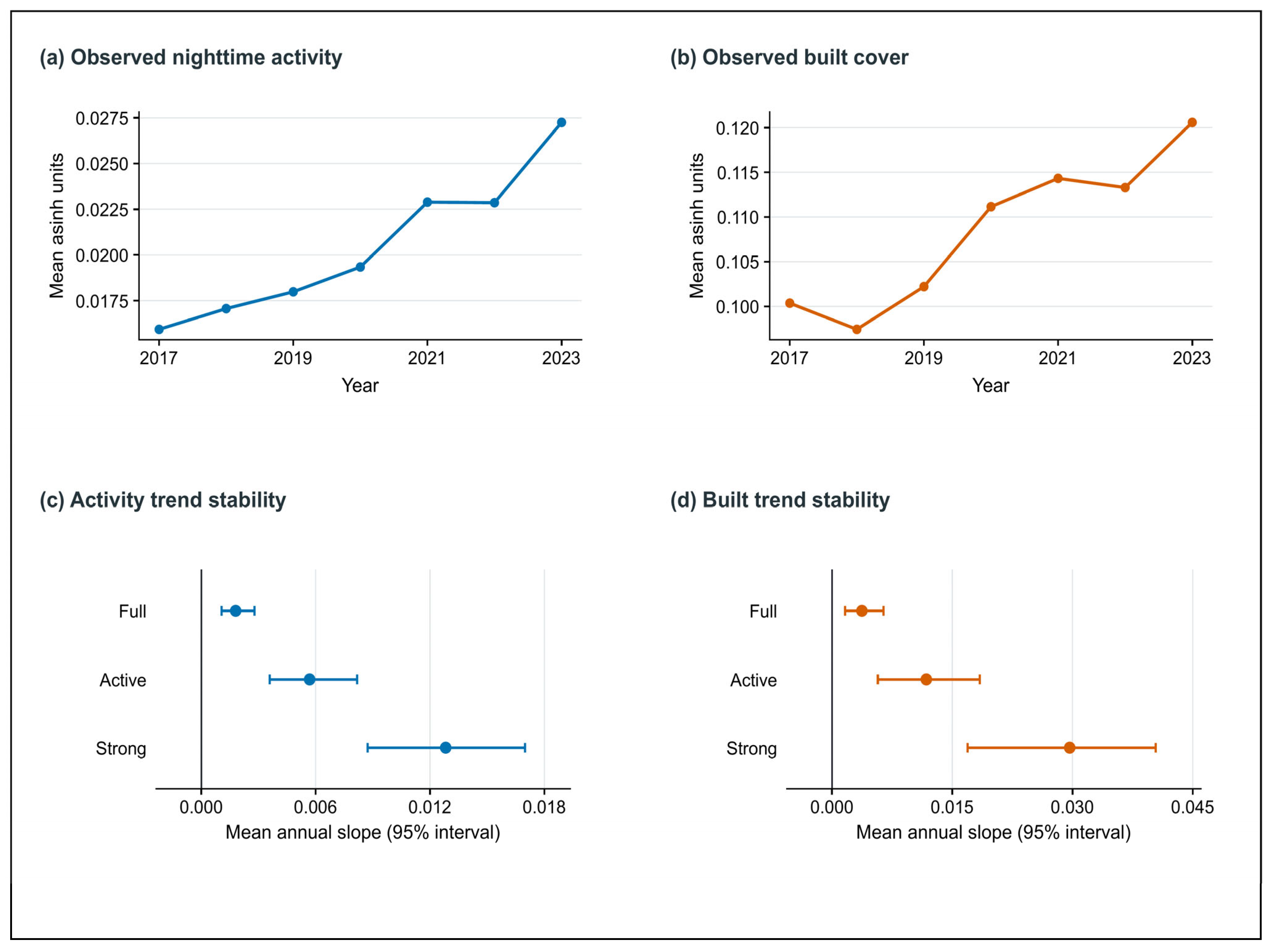
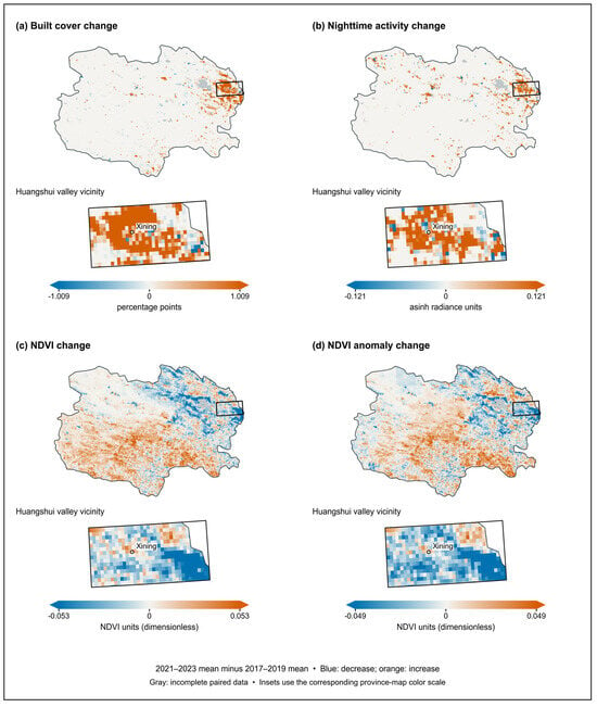
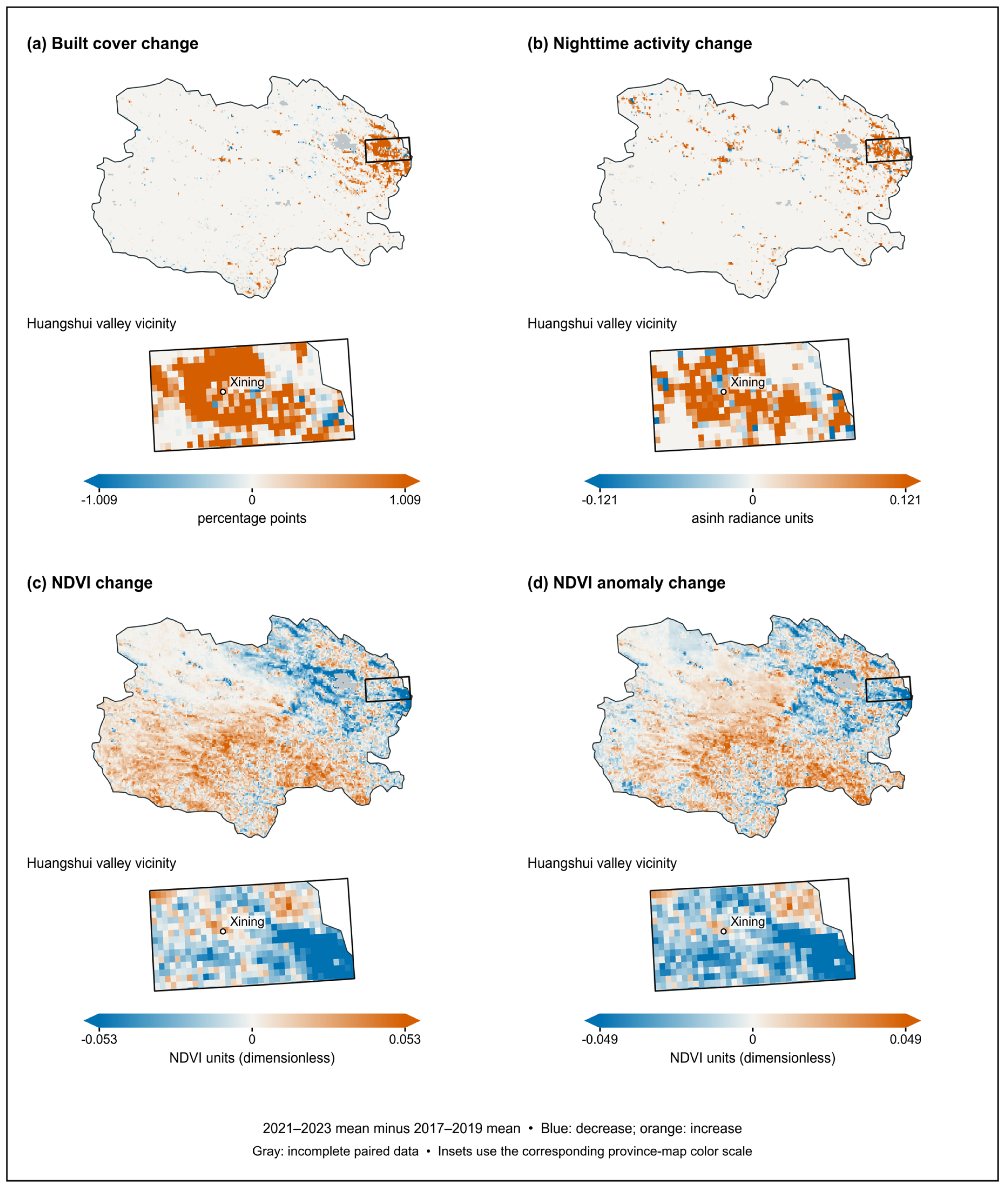
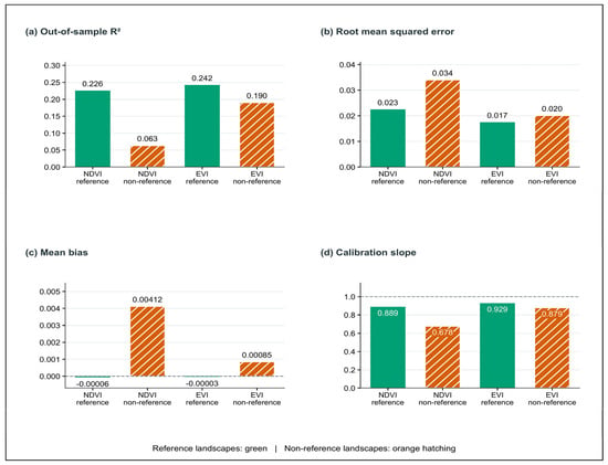
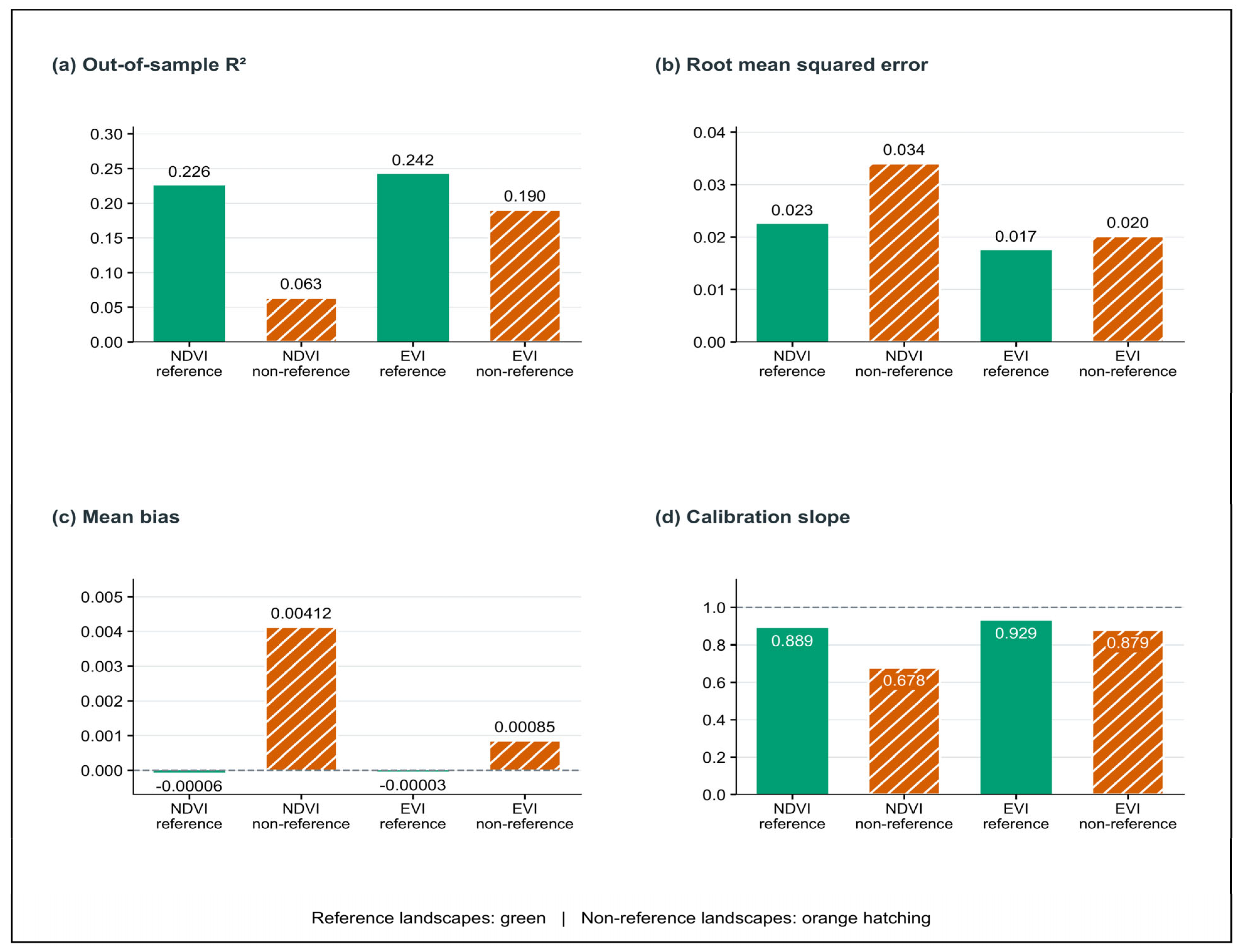
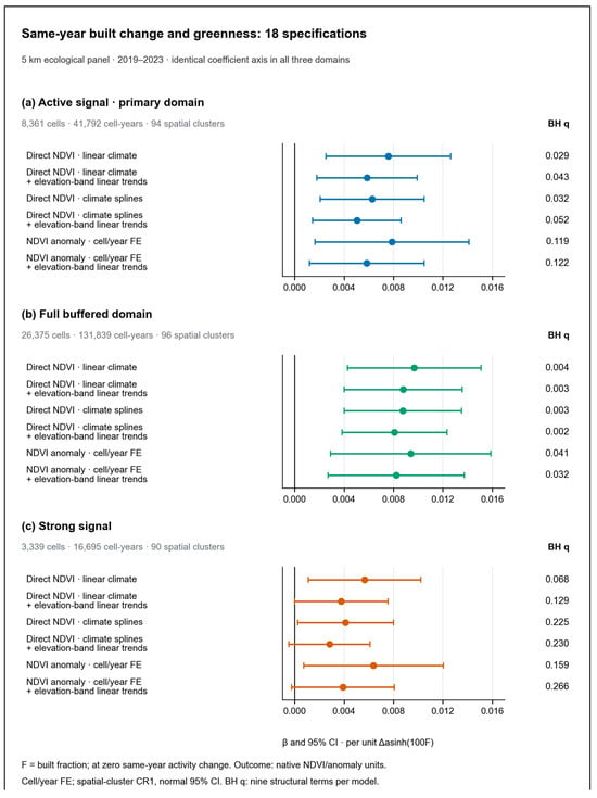
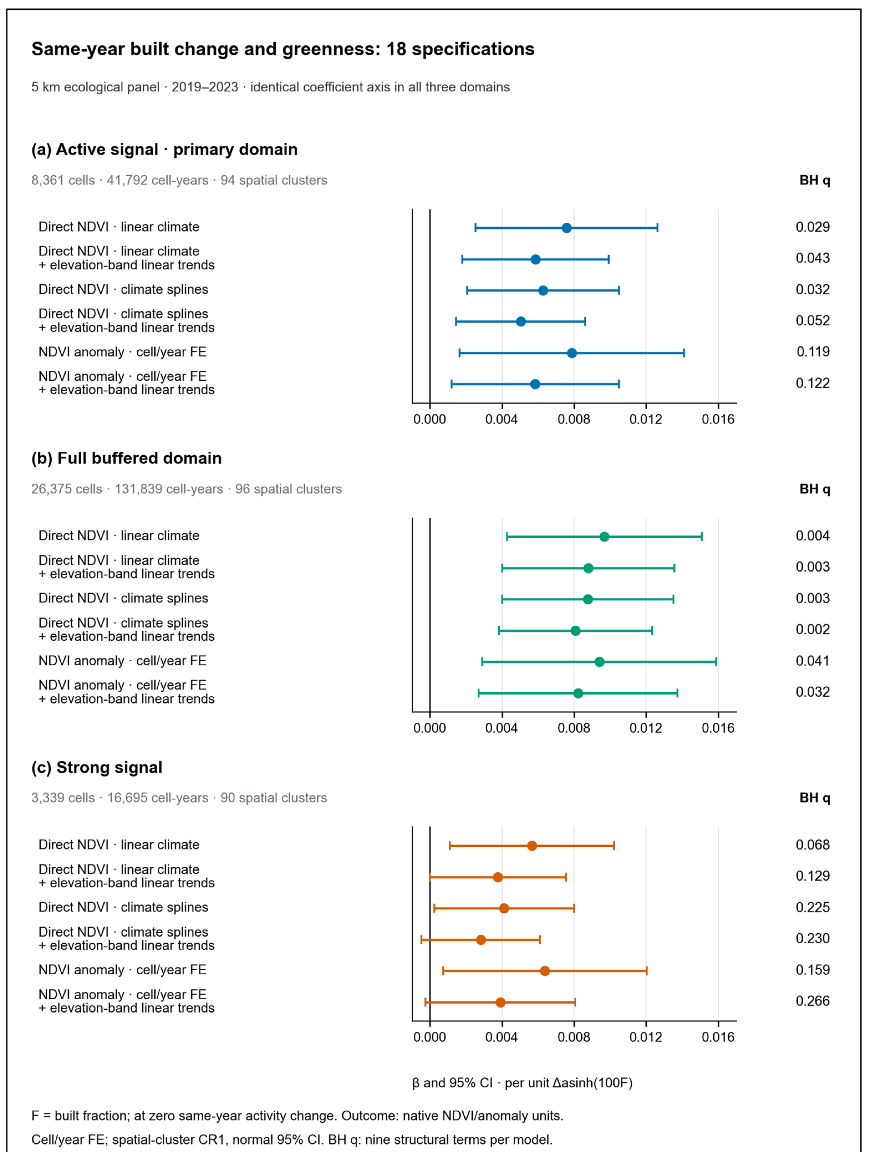
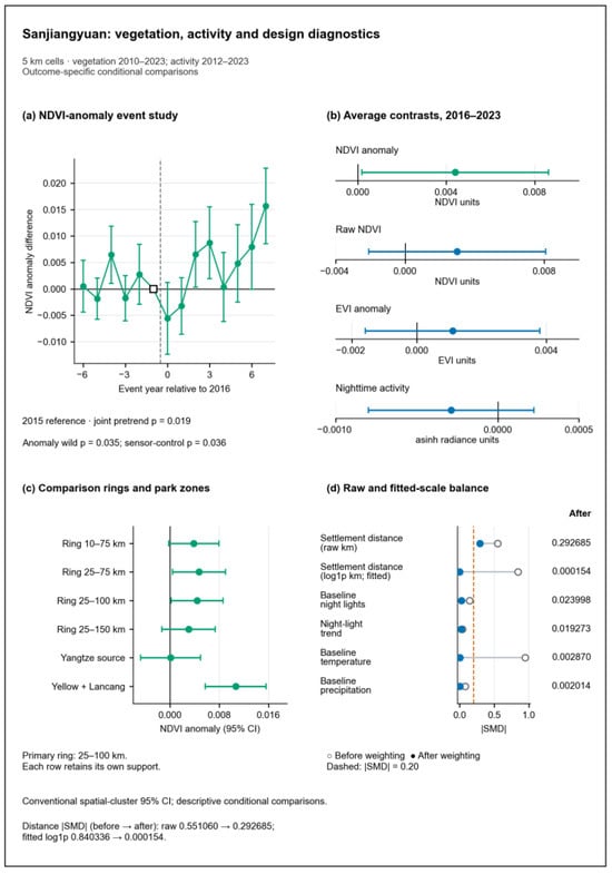
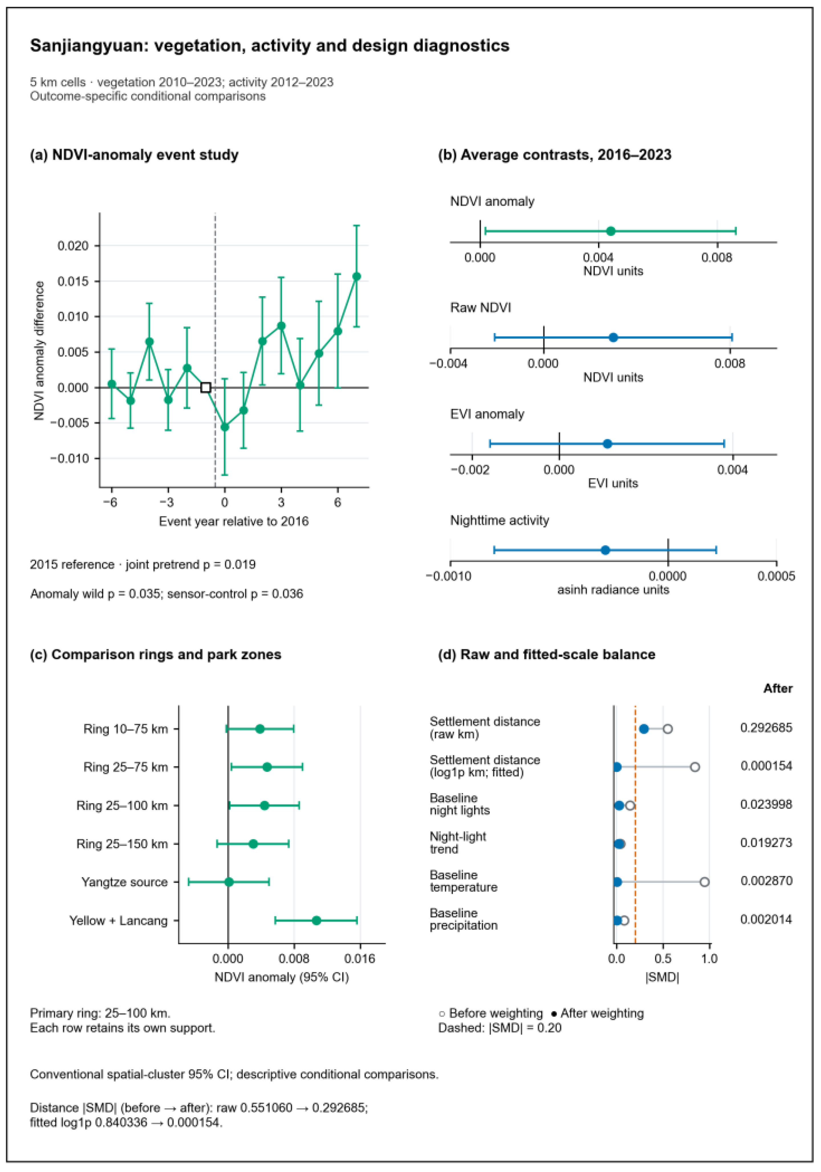
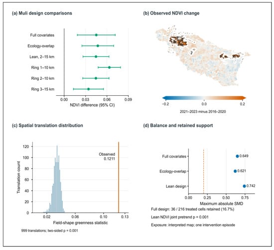
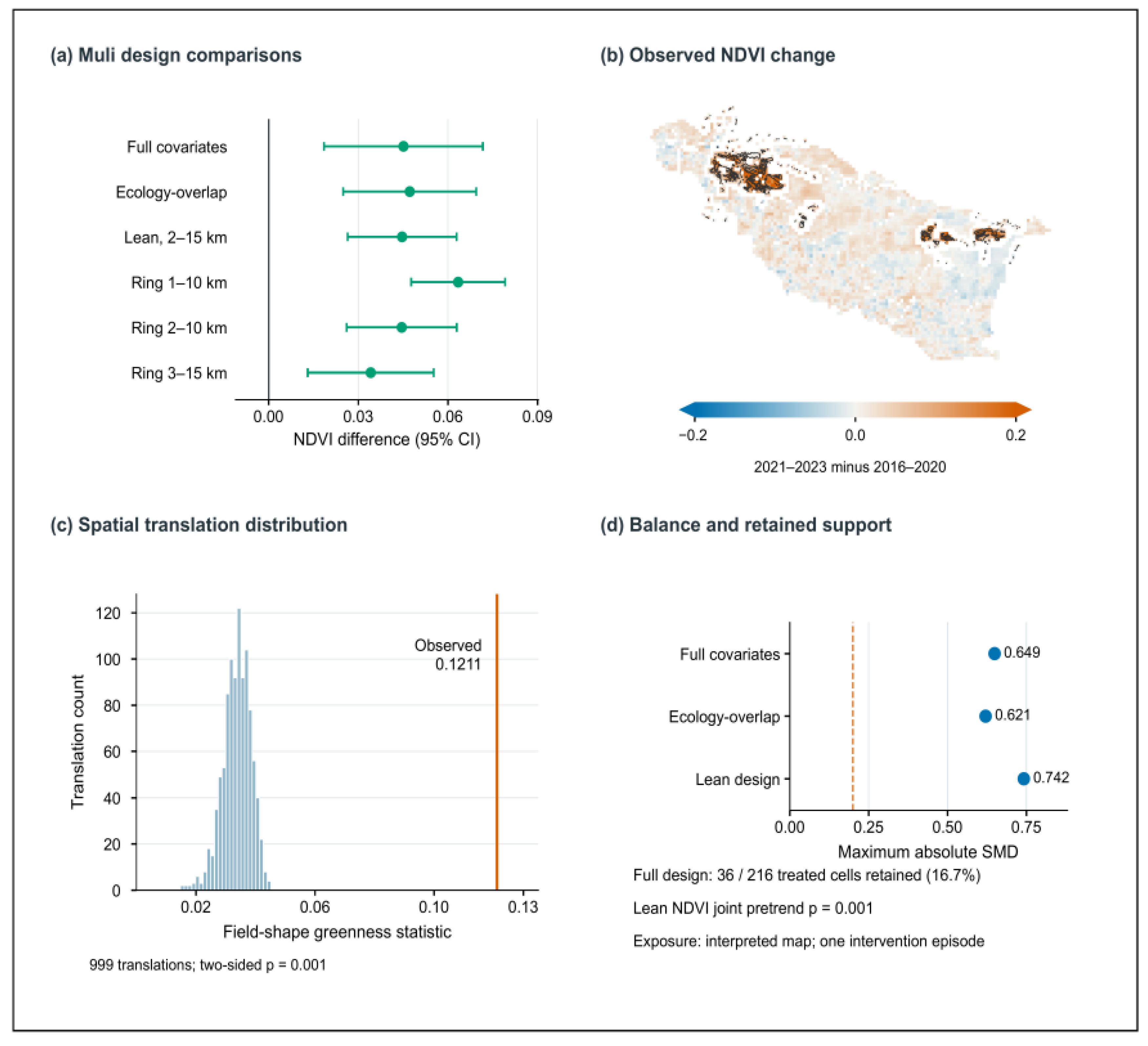

Disclaimer/Publisher’s Note: The statements, opinions and data contained in all publications are solely those of the individual author(s) and contributor(s) and not of MDPI and/or the editor(s). MDPI and/or the editor(s) disclaim responsibility for any injury to people or property resulting from any ideas, methods, instructions or products referred to in the content. |
© 2026 by the authors. Licensee MDPI, Basel, Switzerland. This article is an open access article distributed under the terms and conditions of the Creative Commons Attribution (CC BY) license.