


Abstract
Ammonia is a promising carbon-free marine fuel, but accidental underwater releases of pressurized liquefied ammonia involve complex multiphase flow and phase-change behavior. This study numerically investigated the effects of tank volume on liquefied ammonia release in shallow water. A revised Eulerian multiphase model incorporating temperature-dependent ammonia properties, the Lee evaporation–condensation model, and interfacial surface tension was applied. Grid sensitivity was first evaluated for a 4 m3 tank, and simulations were then performed for 4, 8, and 16 m3 tanks under identical initial pressure and release-opening conditions. Mesh effects were pronounced during the initial transient period but decreased with time; therefore, a Fine mesh with a minimum cell size of 0.01 m was used. Larger tanks depressurized more slowly, sustaining high-velocity liquid release and vapor-phase development for longer periods. Ammonia vapor formed near the release opening and rose buoyantly, producing more extensive and persistent distributions in larger tanks. At approximately 10 s, total gas-phase ammonia normalized by initial stored mass was 5.4%, 6.8%, and 4.2% for the 4, 8, and 16 m3 tanks, respectively. Mass conservation ratios remained close to unity. Thus, tank volume influenced depressurization, release duration, phase-change behavior, and vapor-phase development.
1. Introduction
With the global transition toward carbon neutrality and increasing demands for greenhouse gas (GHG) emission reductions, the maritime sector has been expanding the adoption of low- and zero-carbon fuels as alternatives to conventional fossil fuels [1]. In its revised 2023 greenhouse gas reduction strategy, the International Maritime Organization (IMO) set a target of achieving net-zero greenhouse gas emissions from international shipping by or around 2050 and emphasized the increased use of zero- or near-zero-GHG fuels and energy sources to achieve this goal [1]. Ammonia has attracted attention as a promising next-generation marine fuel because it contains no carbon and therefore does not directly emit carbon dioxide during combustion. Accordingly, safety assessments and studies on ammonia release and dispersion for marine fuel applications have recently been conducted [2,3].
However, ammonia is highly toxic and corrosive, and accidental releases can pose significant risks to human health and the surrounding environment [2,4]. Depending on the storage conditions, liquefied ammonia is maintained under pressurized or refrigerated conditions. When damage occurs to storage tanks or piping systems, ammonia may be released due to the pressure difference between the internal and external environments, accompanied by vaporization caused by depressurization and heat transfer from the surroundings [5,6]. Sivaraman et al. [5] applied a VOF-based CFD model coupled with the Lee evaporation–condensation model to the depressurization and flash boiling of pressurized liquid ammonia and reproduced the experimentally measured final tank pressure and released ammonia mass. Molkov et al. [6] subsequently extended the multiphase modeling of liquid-ammonia release through a piping system and reported agreement with experimental pressure and temperature transients and the total released mass. Although these studies considered atmospheric venting rather than underwater release, they provide experimental support for the application of Lee-based phase-change modeling to the depressurization and phase change in pressurized liquid ammonia. In particular, when liquefied ammonia is released below the water surface, several processes occur simultaneously, including the release of liquid ammonia, generation of ammonia vapor through vaporization, buoyant rise in the vapor phase, and multiphase interaction with the surrounding water. These coupled processes result in complex behavior that differs from that of releases into the atmosphere. Moreover, because of the toxicity of ammonia and the hazards associated with pressurized liquid releases, full-scale release experiments are constrained by safety concerns and experimental scale, particularly under high-pressure conditions [7]. Therefore, numerical approaches are required to complement experimental investigations and to analyze the release and vaporization behavior of liquefied ammonia in marine environments [3,7].
Previous studies on ammonia release have primarily focused on atmospheric dispersion and toxic impact distances following a release, or on computational fluid dynamics (CFD) analyses in which ammonia was assumed to be in the gaseous phase [3,8]. Kim and Jeong [8] used CFD to investigate the dispersion of ammonia vapor and associated toxic impact zones for release scenarios involving onboard ammonia storage tanks. Liu et al. [3] analyzed the effects of release location, release direction, and wind direction on ammonia vapor dispersion during ship-to-ship bunkering. Bouet et al. [9], meanwhile, conducted large-scale release experiments using pressurized liquefied ammonia to investigate two-phase discharge and atmospheric dispersion characteristics. These experimental data have subsequently been used for the validation of ammonia release and dispersion models. However, relatively few studies have addressed vaporization, phase change, and multiphase flow associated with the direct underwater release of pressurized liquefied ammonia in marine environments.
Based on this research need, a previous study numerically investigated the underwater release and vaporization behavior of liquefied ammonia in shallow water using an Eulerian multiphase model consisting of water, air, liquid ammonia, and ammonia vapor together with the Lee phase-change model [10]. Two-dimensional and three-dimensional models were compared under identical conditions, and simulations were subsequently conducted for tank volumes of 4, 8, and 16 m3. Changes in pressure, velocity, volume fraction, and the masses of liquid and vapor-phase ammonia were analyzed to examine the effects of tank volume on release and vaporization behavior [10]. Because the temporal variations in the liquid and vapor ammonia masses were similar between the two-dimensional and three-dimensional models up to approximately 1.8 s, the two-dimensional model was subsequently adopted for the simulations with different tank volumes [10].
However, numerical simulation of underwater liquefied ammonia release is a complex multiphase-flow problem involving rapid pressure changes, phase change, interfaces between dissimilar fluids, and buoyancy-driven flow [5,6]. Therefore, to assess the reliability of numerical results, it is necessary to examine grid sensitivity as well as the treatment of thermophysical properties, turbulence, phase change, and interphase interaction models. In the previous study, local mesh refinement was applied around the release opening and near the water surface; however, the need for additional grid and time-step sensitivity analyses was identified as a limitation of the study [10].
Accordingly, in the present study, a grid sensitivity analysis was first performed for the 4 m3 tank by constructing numerical models with different mesh resolutions and comparing the temporal variations in the internal tank pressure and the masses of liquid and vapor-phase ammonia. In addition, the numerical model used in the previous study was reassessed. Several thermophysical properties of ammonia were modeled as temperature-dependent, and the Continuum Surface Force (CSF) model was introduced to account for surface tension at liquid–gas and liquid–liquid interfaces. Several numerical settings, including coefficients of the Lee phase-change model and the pressure interpolation scheme, were also revised.
The revised numerical model was then applied to simulations of underwater liquefied ammonia release from 4, 8, and 16 m3 tanks under shallow-water conditions. The internal tank pressure, release and flow characteristics, phase change, variations in liquid and vapor ammonia masses, and vaporization behavior were analyzed. Through these analyses, the effects of mesh resolution and numerical-model modifications were examined, and the release and vaporization behavior of liquefied ammonia for different tank volumes was investigated.
2. Numerical Model and Methods
2.1. Governing Equations
To simulate the multiphase flow and phase-change behavior associated with the underwater release of liquefied ammonia, the conservation equations of mass, momentum, and energy were employed as the governing equations. Each phase was treated as a continuous fluid. The mass conservation equation for phase is expressed as
where , , and denote the volume fraction, density, and velocity vector of phase , respectively. and represent the volumetric mass-transfer rates from phase to phase and from phase to phase , respectively, and denotes the external mass source term. The sum of the volume fractions of all phases satisfies:
The same forms of the continuity equation and volume-fraction constraint were also employed in the previous study.
The momentum conservation equation for each phase can be written as
where is the pressure, is the viscous stress tensor of phase , is the gravitational acceleration, represents the interphase force acting between phases and , and denotes the momentum source term. In the previous study, the drag component of the interphase force was calculated using the Schiller–Naumann model. Further details of the interphase interaction models employed in the present study are provided in Section 2.2 and Section 2.4.
To account for heat transfer and latent-heat effects associated with the vaporization and condensation of liquid ammonia, the energy conservation equation for each phase was expressed as
where is the enthalpy of phase , is the effective thermal conductivity, is the temperature, represents the interphase heat-transfer rate, and denotes the energy source term. Interphase heat transfer is determined by the temperature difference between phases and the heat-transfer characteristics at the interface and is calculated together with the interphase mass transfer associated with the vaporization and condensation of ammonia.
2.2. Multiphase Flow Model
An Eulerian multiphase model was employed to simulate the multiphase flow involving water, air, liquid ammonia, and ammonia vapor during the underwater release of liquefied ammonia. In the Eulerian framework, each phase is treated as a continuous interpenetrating fluid, and the spatial distribution of each phase within the computational domain is represented by its volume fraction. The sum of the volume fractions of all phases in each computational cell is equal to unity, and separate mass and momentum conservation equations are solved for each phase. Interphase mass and momentum transfer were accounted for through phase change and interphase forces.
Four phases were considered in the simulation: water, air, liquid ammonia, and ammonia vapor. After liquid ammonia was released from the tank into the surrounding water, ammonia vapor was generated through vaporization depending on the local pressure and temperature conditions. The generated vapor phase then migrated while interacting with the surrounding water and air. To account for momentum exchange arising from the relative velocity between phases, the Schiller–Naumann drag model was employed. The same drag model was also used in the previous study to calculate interphase drag.
The drag force between phase and the dispersed phase is expressed as follows:
where is the drag coefficient, is the characteristic diameter of the dispersed phase, is the volume fraction of the dispersed phase, is the density of the continuous phase, and and are the velocity vectors of the dispersed and continuous phases, respectively.
In the Schiller–Naumann model, the drag coefficient is calculated as a function of the Reynolds number as follows:
This interphase drag formulation was used to calculate momentum transfer arising from the relative motion between different phases. In particular, during the buoyancy-driven rise in ammonia vapor generated underwater, interphase drag between the vapor phase and the surrounding water represents one of the major interaction mechanisms governing the transport behavior of the vapor phase. The Schiller–Naumann model was also employed in the previous study to quantify the drag acting on small bubbles or droplets moving through the surrounding fluid.
2.3. Turbulence Model
During the underwater release of liquefied ammonia, high velocity gradients develop around the release opening due to the pressure difference between the inside and outside of the tank, and turbulent flow is generated through the mixing of the released ammonia with the surrounding water. In this study, the Standard model was employed to simulate the turbulent flow [11,12]. The Standard model calculates the turbulent viscosity using two transport equations for the turbulent kinetic energy, , and the turbulent dissipation rate, , and has been widely applied to various engineering turbulent-flow problems.
The transport equation for the turbulent kinetic energy, , is expressed as follows:
where is the production of turbulent kinetic energy due to the mean velocity gradients, and and are the molecular viscosity and turbulent viscosity, respectively.
The transport equation for the turbulent dissipation rate, , is expressed as follows:
The turbulent viscosity is defined as follows:
The constants of the Standard model were set to [11,12]. Turbulent flow near the walls was treated using the Standard Wall Functions.
In this study, the same Standard turbulence model as that used in the previous study was employed to maintain the basic turbulence-model configuration, while the effects of incorporating temperature-dependent thermophysical properties, interfacial surface tension, and revised numerical settings on the liquefied ammonia release behavior were investigated.
2.4. Phase-Change and Interfacial Models
To simulate vaporization and condensation caused by changes in pressure and temperature during the underwater release of liquefied ammonia, the Lee evaporation–condensation model was employed [13]. The Lee model is an empirical phase-change model that calculates the interphase mass-transfer rate by comparing the temperatures of the liquid and vapor phases with the saturation temperature at the corresponding pressure. It is widely used to simulate vaporization and condensation between liquid and vapor phases in Eulerian multiphase-flow analyses [12,13].
When the temperature of liquid ammonia is higher than the saturation temperature at the corresponding pressure, the mass-transfer rate due to vaporization is calculated as follows:
Conversely, when the temperature of ammonia vapor is lower than the saturation temperature, the mass-transfer rate due to condensation is calculated as follows:
Here, and are the mass-transfer rates per unit volume due to vaporization and condensation, respectively; and are the volume fractions of liquid ammonia and ammonia vapor; and are the densities of the respective phases; and are the temperatures of the respective phases; and is the saturation temperature of ammonia at the corresponding pressure [12,13]. and are the time-relaxation coefficients controlling the rates of vaporization and condensation, respectively, and are empirical parameters of the phase-change model rather than intrinsic thermophysical properties of the material [12]. In this study, the time-relaxation coefficients for vaporization and condensation were both set to 0.5 for all simulation conditions.
The time-relaxation coefficients are problem-dependent empirical parameters rather than intrinsic thermophysical properties. Previous ammonia phase-change studies have reported substantially different coefficient ranges depending on the flow configuration and operating conditions. For example, Sivaraman et al. [5] calibrated values in the range of 0.007–0.1 s−1 for liquid-ammonia tank venting, whereas values around 0.5 s−1 for evaporation have also been reported for ammonia phase-change simulations in thermosyphon applications [14]. In the present study, a fixed value of 0.5 s−1 was applied consistently to all tank-volume cases to maintain identical phase-change-model settings for the comparative analysis. This value was not calibrated specifically for the present underwater-release configuration.
The saturation temperature of ammonia was set to vary with the local pressure, and the relationship between saturation pressure and saturation temperature was obtained from the ammonia property data provided by the National Institute of Standards and Technology (NIST) [15]. The same data were also used in the previous study to account for the variation in saturation temperature with pressure.
During the release of liquefied ammonia into water, interfaces are formed among water, air, liquid ammonia, and ammonia vapor. To account for surface-tension effects at these phase interfaces in the momentum-transfer process, the Continuum Surface Force (CSF) model was applied [16]. In the CSF model, the surface tension acting at an interface is converted into a volumetric force term in the momentum equation. The interface orientation and curvature are determined from the spatial variation in volume fraction, and the resulting quantities are used to account for surface-tension effects [12,15]. In the Fluent model used in this study, Surface Tension Force Modeling was enabled and the CSF model was applied.
The pressure difference caused by surface tension between two fluids is expressed by the Young–Laplace relation as follows:
where is the surface tension coefficient between the two phases , and is the curvature of the interface. The interface normal vector can be defined using the gradient of the volume fraction as follows:
The curvature of the interface is calculated using the unit normal vector as follows [12,15]:
The calculated interface curvature and surface tension coefficient were then used to incorporate the force due to surface tension into the momentum equation.
Constant surface tension coefficients were applied to the major phase pairs, as summarized in Table 1. The surface tension of liquid ammonia varies with temperature, and Kim et al. [17] reported a value of approximately 0.0217 N/m at 20 °C. Yang et al. [18] applied a surface tension coefficient of 0.025 N/m to the interface between liquid ammonia and ammonia vapor in a CFD study of an ammonia boiler. Considering the reported surface tension of liquid ammonia near room temperature, surface tension coefficients of 0.021 N/m and 0.025 N/m were applied to the ammonia vapor–liquid ammonia and air–liquid ammonia interfaces, respectively. Meanwhile, the surface tension at the water–liquid ammonia interface is affected by factors such as composition and temperature, and experimental data have been reported to be limited [19]. Therefore, a constant surface tension coefficient of 0.035 N/m was specified as the model input for the water–liquid ammonia interface. A temperature- and composition-dependent interfacial-tension model was not introduced because corresponding data are limited, particularly for the water–liquid ammonia interface. Therefore, representative constant values based on the available literature were applied consistently to all tank-volume cases to maintain identical interfacial-model settings for the comparative analysis.
Table 1.
Surface tension coefficients applied to major phase pairs.
In this study, the Lee model was used to calculate the mass transfer associated with vaporization and condensation between liquid ammonia and ammonia vapor, while the CSF model was additionally employed to account for surface-tension effects at the interfaces between liquid ammonia and the surrounding fluids. The same phase-change and interfacial-model conditions were applied to all tank volumes of 4, 8, and 16 m3.
2.5. Thermophysical Properties of Ammonia
During the release and phase-change processes of liquefied ammonia, pressure and temperature vary with time, and consequently, the properties of liquid ammonia and ammonia vapor may also change [15]. In particular, during the underwater release of pressurized liquefied ammonia considered in this study, temperature changes occur due to the decrease in tank pressure and vaporization near the release opening. Therefore, the temperature dependence of major thermophysical properties was incorporated into the numerical model.
The densities of liquid ammonia and ammonia vapor were defined as temperature-dependent properties. For liquid ammonia, a total of 22 temperature–density data points were applied over the range of 196–399.09 K, and the density between adjacent data points was calculated by linear interpolation. The density of liquid ammonia was set to 731.22 kg/m3 at 196 K and decreased with increasing temperature to 350.73 kg/m3 at 399.09 K. For ammonia vapor, six temperature–density data points were applied over the range of 240.15–313.15 K, with linear interpolation between adjacent data points. The density of ammonia vapor was 7.25 kg/m3 at 240.15 K and 5.67 kg/m3 at 313.15 K. In the previous study, constant density values were applied to both liquid ammonia and ammonia vapor, whereas in the present study, the densities were allowed to vary in response to temperature changes occurring during the release and phase-change processes.
The constant-pressure specific heat, , of ammonia vapor was defined using fourth-order polynomials for different temperature ranges to account for its temperature dependence [12]. The relationship between the constant-pressure specific heat and temperature is expressed as follows:
where is the temperature (K), and the unit of is J/(kg·K). The applied temperature ranges and polynomial coefficients are given in Table 2.
Table 2.
Polynomial coefficients for calculating the constant-pressure specific heat of ammonia vapor over different temperature ranges.
For liquid ammonia, constant values of 4756 J/(kg·K), 0.526 W/(m·K), and 1.45 × 10⁻⁴ kg/(m·s) were applied for the constant-pressure specific heat, thermal conductivity, and dynamic viscosity, respectively. For ammonia vapor, constant values of 0.0247 W/(m·K) and 1.015 × 10⁻⁵ kg/(m·s) were applied for the thermal conductivity and dynamic viscosity, respectively. The major ammonia properties and their treatments in the numerical model are summarized in Table 3.
Table 3.
Major properties of ammonia applied in the numerical analysis.
Thus, temperature dependence was incorporated into the densities of liquid ammonia and ammonia vapor and the constant-pressure specific heat of ammonia vapor, while representative constant values corresponding to the simulation conditions were applied to the remaining major properties. The same thermophysical-property settings were applied to all tank volumes of 4, 8, and 16 m3.
2.6. Computational Domain and Initial and Boundary Conditions
A two-dimensional computational domain was constructed to simulate the underwater release of pressurized liquefied ammonia from a storage tank under shallow-water conditions. The computational domain consisted of a water region and an air region above the water surface, with the ammonia storage tank positioned below the water surface. The top of the tank was located 0.5 m below the water surface, and the center of the release opening was located 3 m below the water surface. The size of the release opening was set to 0.2 m. The same computational domain and release location were used in the previous study.
The computational domain was designed to analyze vaporization and buoyancy-driven upward transport following the release of liquefied ammonia. Seabed topography and interactions with the seabed were not considered separately. Therefore, the bottom of the computational domain was specified as a boundary limiting the analysis region.
The tank height was maintained at 4 m for all cases, while the horizontal length was varied to construct three tank-volume cases of 4, 8, and 16 m3 for comparison of the effects of tank volume. The horizontal lengths of the tanks were 1, 2, and 4 m, respectively, while the height was fixed at 4 m for all cases. The size and location of the release opening were kept identical for all tank volumes so that the effect of tank volume could be compared under the same release conditions. The analysis conditions for the three tank volumes are summarized in Table 4.
Table 4.
Analysis conditions for different tank volumes.
At the initial state, the region outside the tank below the water surface was filled with water, while the region above the water surface was filled with air. The tank was initially filled with liquid ammonia. No liquid ammonia or ammonia vapor was present outside the tank in the initial state. The initial volume-fraction distributions of water, air, liquid ammonia, and ammonia vapor were specified in the same manner as in the previous study.
The initial absolute pressure inside the tank was set to 8 bar, and the initial temperature of liquid ammonia was set to 15 °C. The initial temperatures of the water and air were set to 24.8 °C and 20 °C, respectively. These initial conditions were maintained identical to those used in the previous study. In addition, a gravitational acceleration of 9.81 m/s2 was applied in the vertically downward direction to account for the buoyant rise in ammonia vapor and fluid motion following the release.
The upper boundary of the computational domain was specified as an open boundary connected to the ambient atmosphere, with an atmospheric pressure of 101,325 Pa. The outer boundaries of the computational domain, except for the upper boundary, and the walls of the storage tank were specified as impermeable solid walls. No-slip and adiabatic conditions were applied at the walls. These boundary conditions were also maintained identical to those used in the previous study.
Except for the tank volume, the size and location of the release opening, initial pressure and temperature, and external fluid conditions were kept identical among all cases. This allowed the relative differences in pressure reduction, release behavior, and phase-change characteristics among the different tank volumes to be compared. The computational domain, boundary conditions, and initial phase distributions are shown in Figure 1.
Figure 1.
Computational domain, boundary conditions, and initial phase distribution for the 2D numerical simulation of the 8 m3 tank: (a) computational domain and boundary conditions, and (b) initial volume-fraction distributions of water, air, liquid ammonia, and ammonia vapor.
2.7. Numerical Methods
Numerical simulations were performed using ANSYS Fluent 2026 R1 (ANSYS, Inc., Canonsburg, PA, USA). A pressure-based transient numerical analysis was performed to investigate the temporal evolution of phase change and multiphase flow associated with the underwater release of liquefied ammonia. The Coupled algorithm was employed for pressure–velocity coupling, and spatial gradients were evaluated using the least-squares cell-based method based on the values in the neighboring computational cells [12].
The PRESTO! (PREssure STaggering Option) scheme was applied for pressure interpolation. The convective terms of the momentum, volume fraction, turbulent kinetic energy, turbulent dissipation rate, and energy equations were discretized using the first-order upwind scheme. The temporal terms were discretized using the first-order implicit scheme. The underwater release of liquefied ammonia considered in this study is a highly transient multiphase-flow problem involving a rapid initial discharge caused by the large pressure difference, phase change, and simultaneous variations in the volume fractions of the phases. Therefore, first-order discretization schemes were employed, considering numerical stability and convergence during the initial transient period [12]. The same discretization schemes were applied to all tank volumes to prevent differences in numerical settings from affecting the comparison among the different tank-volume cases. However, first-order discretization schemes introduce numerical diffusion, which can smooth steep velocity and volume-fraction gradients and damp local peak values and small-scale flow structures. Therefore, detailed jet boundaries, local interface structures, and vortical features should be interpreted with consideration of this numerical limitation.
The time step for the transient simulations was set to 5 × 10⁻⁴ s, with a maximum of 20 iterations performed at each time step. The residual convergence criterion for each governing equation was set to 1 × 10⁻³. The same time step and iteration settings were applied to all simulations for the 4, 8, and 16 m3 tanks. A time step of 5 × 10⁻⁴ s was also used for the transient simulations in the previous study.
The major numerical methods and solution settings used in the present study are summarized in Table 5.
Table 5.
Numerical methods and solution settings used in the present analysis.
The same numerical settings were applied to all tank volumes to compare the release and phase-change characteristics as a function of tank volume. The raw numerical data used to generate the quantitative figures presented in Section 3 and Section 4 are provided in Supplementary File S1.
3. Grid Sensitivity Analysis
3.1. Mesh Configuration
A grid sensitivity analysis was performed for the 4 m3 tank to examine the effect of mesh size on the numerical results. The computational domain, initial and boundary conditions, thermophysical properties, and multiphase-flow and phase-change models were maintained as identical, while only the mesh size was varied to compare the simulation results.
The reference mesh was constructed using local refinement, with relatively fine cells applied around the release opening and near the water surface. In particular, a minimum cell size of 0.01 m was applied around the 0.2 m release opening to resolve the initial high-velocity release and phase-change behavior. The same minimum cell size was also used in the previous study, in which local mesh refinement was applied around the release opening and near the water surface.
For the grid sensitivity analysis, three meshes were constructed by progressively increasing the minimum cell size by a factor of two, resulting in minimum cell sizes of 0.01, 0.02, and 0.04 m. In a two-dimensional analysis, when the representative cell length is doubled, the total number of cells over the same area theoretically decreases to approximately one-quarter, while a fourfold increase in cell length reduces the total cell count to approximately one-sixteenth. The actual total numbers of cells were 659,167, 166,332, and 43,935, corresponding to approximately 100%, 25.2%, and 6.7% of the Fine mesh cell count, respectively. These values were generally consistent with the expected mesh-refinement relationship. Hereafter, the three meshes are referred to as the Fine, Medium, and Coarse meshes, respectively. Considering the release-opening size of 0.2 m, the minimum-cell-size regions corresponded to approximately 20, 10, and 5 computational cells across the opening for the Fine, Medium, and Coarse meshes, respectively. The local mesh configurations are shown in Figure 2, and the corresponding mesh statistics are summarized in Table 6.
Figure 2.
Local mesh configurations around the release opening for the (a) Fine, (b) Medium, and (c) Coarse meshes. The red arrows indicate the release opening.
Table 6.
Mesh configurations for the grid sensitivity analysis.
The same time step of 5 × 10⁻⁴ s and the same numerical methods described in Section 2.7 were applied to all three mesh cases. This allowed the effects of spatial mesh size on the internal tank pressure and the masses of liquid ammonia and ammonia vapor to be evaluated while maintaining identical temporal discretization and numerical-solution settings.
3.2. Pressure Variation for Different Mesh Resolutions
Figure 3 shows the temporal variation in the absolute pressure inside the 4 m3 tank for different mesh resolutions. To clearly present the overall trend in pressure variation, a 101-point moving median filter was applied to reduce instantaneous numerical oscillations. With a time step of 5 × 10⁻⁴ s, the 101-point window corresponds to a time interval of approximately 0.0505 s. The moving median filter was applied only for visualization of the pressure histories, and the original simulation data were used for all quantitative comparisons. The original data at the beginning and end of the simulation, where a complete filtering window was not available, were retained.
Figure 3.
Time histories of the absolute pressure inside the tank for different mesh resolutions.
For all mesh resolutions, the initial absolute pressure inside the tank was approximately 8.01 bar, and a rapid pressure decrease occurred immediately after the release began due to the pressure difference between the inside and outside of the tank. During the initial transient period, some differences in the rate of pressure decrease were observed depending on the mesh resolution. In particular, the initial pressure decrease was relatively faster for the Fine mesh than for the Medium and Coarse meshes. At 0.1 s, the absolute pressures for the Fine, Medium, and Coarse meshes were approximately 2.78, 4.66, and 4.66 bar, respectively. Thereafter, the pressure differences among the three meshes gradually decreased.
At approximately 1 s, the absolute pressures for the Fine, Medium, and Coarse meshes were approximately 1.40, 1.29, and 1.31 bar, respectively. Subsequently, all three cases exhibited similar pressure variations within a range of approximately 1.2–1.3 bar. For the Coarse mesh, a temporary pressure fluctuation occurred during the initial transient period but rapidly stabilized thereafter, and after approximately 2 s, the pressure variations for the three meshes were generally similar.
At the end of the simulation, t = 10 s, the absolute pressures for the Fine, Medium, and Coarse meshes were approximately 1.27, 1.26, and 1.27 bar, respectively. Therefore, although differences among the mesh resolutions were observed during the rapid depressurization immediately after the release began, these differences decreased with time, and the pressures tended to converge toward similar levels.
3.3. Ammonia Mass Variation
Figure 4 shows the temporal variations in the masses of liquid ammonia and ammonia vapor inside the tank for different mesh resolutions. The initial mass of liquid ammonia was approximately 2500.65 kg for all mesh resolutions and decreased rapidly after the release began due to outflow from the tank and phase change.
Figure 4.
Time histories of ammonia mass inside the tank for different mesh resolutions.
As shown in Figure 4a, the mass of liquid ammonia exhibited a similar trend for all mesh resolutions, decreasing rapidly during approximately the first 1 s after the onset of the release and then decreasing more gradually with time. Differences among the mesh resolutions were observed during the initial transient period. At 1 s, the masses of liquid ammonia for the Fine, Medium, and Coarse meshes were approximately 1598, 1431, and 1359 kg, respectively. Thereafter, the decrease in liquid ammonia mass proceeded more gradually, and the corresponding masses at 10 s were approximately 1321, 1344, and 1300 kg, respectively. Based on the initial mass, approximately 52–54% of the liquid ammonia remained inside the tank at the end of the simulation.
As shown in Figure 4b, the mass of ammonia vapor increased rapidly immediately after the release began due to the vaporization of liquid ammonia. At 1 s, the masses of ammonia vapor for the Fine, Medium, and Coarse meshes were approximately 10.83, 13.42, and 14.65 kg, respectively. As with the liquid ammonia mass, relatively large differences among the mesh resolutions were observed during the initial transient period. Thereafter, the rate of change in the vapor mass decreased substantially, and the masses at 10 s were approximately 13.60, 13.95, and 14.19 kg, respectively. Consequently, during the later stage of the simulation, the differences in ammonia vapor mass among the three mesh resolutions were smaller than those observed during the initial transient period.
For the Fine mesh, the ammonia vapor mass remained nearly constant after approximately 4 s, whereas for the Coarse mesh, it showed a slight decrease after the initial increase. For the Medium mesh, a gradual increase continued until the end of the simulation. Despite these detailed differences, all mesh resolutions exhibited the same overall behavior: a rapid decrease in liquid ammonia mass and an increase in ammonia vapor mass during the initial stage of the release, followed by a reduction in the rates of mass change.
3.4. Grid Sensitivity Assessment
To quantitatively evaluate the differences in the numerical results with mesh resolution, the relative differences for the Medium and Coarse meshes were calculated with respect to the Fine mesh. The relative difference was defined as follows:
where represents the physical quantity calculated using the Medium or Coarse mesh, and is the value calculated using the Fine mesh at the same time. To compare both the initial transient behavior and the subsequent evolution, the absolute pressure inside the tank and the masses of liquid ammonia and ammonia vapor were compared at 1, 5, and 10 s.
The calculated relative differences are summarized in Table 7.
Table 7.
Relative differences in the numerical results for the Medium and Coarse meshes with respect to the Fine mesh.
At the initial stage of the release, 1 s, relatively large differences were observed among the mesh resolutions. In particular, the ammonia vapor masses obtained with the Medium and Coarse meshes differed from those obtained with the Fine mesh by approximately 23.9% and 35.2%, respectively, indicating that the initial transient period, during which rapid depressurization and phase change occur simultaneously, was relatively sensitive to the spatial mesh resolution. The liquid ammonia mass also showed differences of approximately 10.4% and 15.0% at 1 s, while the differences in pressure were approximately 6–7%.
The relatively large mesh sensitivity during the initial transient period can be attributed to the highly localized and rapidly evolving flow near the release opening. Immediately after the onset of the release, steep pressure and velocity gradients, rapid phase change, and strong variations in the phase interfaces occur simultaneously within a limited region around the 0.2 m opening. Because the Fine, Medium, and Coarse meshes resolve this region with approximately 20, 10, and 5 cells across the opening, respectively, the representation of these localized gradients and interphase mass transfer is more sensitive to mesh resolution during the early stage of the release.
In contrast, the differences among the meshes decreased substantially with time. At 5 s, the relative differences were within approximately 1% for the absolute pressure, 4.4% for the liquid ammonia mass, and 5.9% for the ammonia vapor mass. At 10 s, the corresponding differences were within 1%, approximately 1.8%, and approximately 4.3%, respectively. Thus, the effect of mesh resolution was relatively pronounced during the rapid initial transient period but decreased with time for both the pressure and ammonia mass.
Because this study aims to analyze both the initial pressure decrease and phase-change behavior following the release, the Fine mesh, which provides finer resolution of the initial transient period, was employed for the subsequent simulations. However, relatively large differences among the mesh resolutions were observed during the initial transient period, and monotonic convergence was not obtained for all physical quantities and sampling times. Therefore, the present analysis should be interpreted as a grid-sensitivity assessment rather than a demonstration of asymptotic grid convergence or strict grid independence. Among the three meshes examined, the Fine mesh was selected as the most highly resolved configuration for the subsequent tank-volume simulations.
4. Underwater Release Behavior of Liquefied Ammonia Using the Revised Numerical Model
4.1. Pressure Variation for Different Tank Volumes
Figure 5 shows the temporal variations in the absolute pressure inside the 4, 8, and 16 m3 tanks obtained using the revised numerical model. The same 101-point moving median filter described in Section 3.2 was applied only for visualization of the pressure histories to reduce instantaneous numerical oscillations and to facilitate comparison of the overall pressure-decrease trends.
Figure 5.
Time histories of the absolute pressure inside the tank for different tank volumes.
For all simulation cases, the initial absolute pressure inside the tank was set to approximately 8.01 bar, and rapid depressurization occurred immediately after the release began due to the pressure difference between the inside and outside of the tank. However, the rate and duration of depressurization differed markedly depending on the tank volume. For the 4 m3 tank, the pressure decreased most rapidly immediately after the onset of the release, reaching approximately 1.3–1.4 bar within about 1 s. In contrast, the 8 and 16 m3 tanks contained larger amounts of liquefied ammonia, resulting in a more gradual decrease in pressure and a delayed arrival at the low-pressure region.
Temporary pressure fluctuations were observed during the initial depressurization process for the 8 and 16 m3 tanks. Because these fluctuations may include the effects of numerical oscillations arising from the transient multiphase-flow and phase-change calculations, the results were compared primarily on the basis of the overall pressure-decrease trend rather than individual instantaneous values.
After approximately 3 s, the absolute pressures inside all three tanks were at similar levels, within approximately 1.2–1.4 bar, and thereafter changed gradually without substantial differences until 10 s. Thus, although the initial depressurization proceeded more slowly with increasing tank volume, all three cases tended to approach similar pressure levels close to the external hydrostatic pressure after sufficient time had elapsed.
4.2. Release and Flow Characteristics
Figure 6 shows the velocity magnitude distributions of liquid ammonia at t = 0.1, 1.0, and 3.0 s for the 4, 8, and 16 m3 tanks. During the initial stage of the release, liquid ammonia was discharged at high velocity through the release opening in all three cases, forming a distinct jet immediately downstream of the opening. The initial jet developed primarily in the horizontal direction and, with time, exhibited an upward-curving flow structure due to interactions with the surrounding fluid and buoyancy effects.
Figure 6.
Temporal evolution of velocity magnitude contours of liquid ammonia for the 4, 8, and 16 m3 tanks. The tank outline and release opening are also shown for clarity. The upper limit of each velocity-magnitude color bar represents the maximum velocity for the corresponding tank-volume case and time instant.
For the 4 m3 tank, the initial depressurization proceeded relatively rapidly, and the high-velocity liquid-phase flow tended to weaken within a short period. In contrast, for the 8 and 16 m3 tanks, the internal tank pressure was maintained for a relatively longer period, resulting in a more sustained liquid ammonia jet and a greater spatial extent of plume development outside the release opening. In particular, for the 16 m3 tank at 3.0 s, liquid ammonia spread over a wider region and formed complex vortex and recirculation structures.
These results suggest that, as the tank volume increases, the release of liquid ammonia can be sustained for a longer period due to the greater initial stored mass and the resulting pressure-retention effect, allowing the flow structure outside the tank to develop over a larger region. However, different velocity-magnitude ranges were used for the individual contours because the maximum velocities differed substantially among the tank-volume cases and time instants. The upper limit of each color bar corresponds to the maximum velocity obtained for the corresponding case and time. For example, at 1.0 s, the maximum velocities were approximately 6.8, 24.1, and 31.2 m/s for the 4, 8, and 16 m3 tanks, respectively. Applying a common scale based on the largest value would substantially reduce the visibility of the flow structures in the lower-velocity cases. Therefore, the individual scales were retained to visualize the spatial development of the flow, while the color-bar maxima allow quantitative comparison of the maximum velocity. Because the present simulations are two-dimensional, the velocity contours are used to compare the relative planar development of the release flow among the tank-volume cases; the detailed vortex structures and spatial spreading should not be interpreted as quantitative representations of the corresponding three-dimensional flow field.
4.3. Phase Change and Volume-Fraction Variation
Figure 7 shows the volume-fraction distributions of ammonia vapor at t = 0.1, 1.0, and 3.0 s after the release for the 4, 8, and 16 m3 tanks. All contours are presented using the same volume-fraction range of 0–1 to allow comparison of the relative changes in the vapor-phase distribution with time and tank volume.
Figure 7.
Temporal evolution of ammonia vapor volume fraction for the 4, 8, and 16 m3 tanks at 0.1, 1.0, and 3.0 s.
Immediately after the release, at t = 0.1 s, a localized ammonia vapor region formed near the release opening for all tank volumes. At this time, flash vaporization due to depressurization had begun, but the vapor phase remained confined to a limited region around the release opening. Thus, during the initial stage, ammonia vapor existed as small bubble-like structures near the release opening rather than spreading throughout the computational domain.
At t = 1.0 s, the ammonia vapor region expanded into the surrounding domain together with the release jet and developed a distinct vortical structure. For the 4 m3 tank, the vapor phase exhibited a relatively small curled structure near the release opening and expanded upward and forward, whereas larger vapor-phase regions were formed for the 8 and 16 m3 tanks. This behavior is attributed to the relatively slower depressurization with increasing tank volume, which allows the release and vaporization processes to continue for a certain period under a relatively high pressure difference. Accordingly, at the same time, the spatial extent of the vapor-phase distribution was generally greater for the 8 and 16 m3 tanks than for the 4 m3 tank.
At t = 3.0 s, the differences among the tank volumes became more pronounced. For the 4 m3 tank, ammonia vapor extended forward from the release opening but remained distributed within a relatively limited region, with a more elongated structure than that observed during the initial stage of the release. In contrast, for the 8 and 16 m3 tanks, ammonia vapor spread over wider regions and formed complex vortex and recirculation structures. In particular, the 16 m3 tank showed a more spatially extended and persistent vapor-phase region within the two-dimensional computational domain. This is because a larger tank contains a greater amount of liquid ammonia and sustains the release for a longer period, thereby enhancing the generation and development of the vapor phase.
These results are consistent with the pressure variation and velocity-field results presented above. Specifically, in the smaller tank, rapid initial depressurization caused the release intensity and vapor-phase development to weaken within a relatively short period. In contrast, the larger tanks underwent more gradual depressurization, allowing the generation and outward spread of ammonia vapor to continue for a longer period. Therefore, for the underwater release of liquefied ammonia in shallow water, tank volume was found to be a major factor influencing not only the amount of ammonia vapor generated but also the spatial development of the vapor phase within the two-dimensional computational framework.
4.4. Ammonia Mass Inside the Tank
Figure 8 shows the temporal variations in the masses of liquid ammonia and ammonia vapor inside the tank for different tank volumes. The initial masses of liquid ammonia were approximately 2500.65, 5001.30, and 10,002.60 kg for the 4, 8, and 16 m3 tanks, respectively, and decreased rapidly after the release began in all cases. In particular, the liquid ammonia mass decreased substantially during the initial depressurization period of approximately 1–3 s, after which the rate of decrease became relatively gradual.
Figure 8.
Time histories of ammonia mass inside the tank for different tank volumes.
At 1 s, the masses of liquid ammonia inside the 4, 8, and 16 m3 tanks were approximately 1598, 3121, and 7596 kg, respectively. In particular, for the 16 m3 tank, a relatively large amount of liquid ammonia remained inside the tank compared with its initial mass at the same time, which is consistent with the differences in depressurization rate observed among the tank volumes. After approximately 3 s, the rate of decrease in liquid ammonia mass was substantially reduced for all three cases, and at around 10 s, the corresponding masses were approximately 1.32 × 10³, 2.55 × 10³, and 5.44 × 10³ kg, respectively.
The mass of ammonia vapor inside the tank increased rapidly immediately after the release began. For the 4 m3 tank, it reached approximately 13 kg after about 2 s and then remained nearly constant. For the 8 and 16 m3 tanks, the ammonia vapor mass also increased continuously during the initial stage, reached maximum values of approximately 31 and 58 kg, respectively, and then gradually decreased. At around 10 s, the ammonia vapor masses were approximately 13.6, 28.8, and 55.7 kg for the 4, 8, and 16 m3 tanks, respectively.
Thus, during the initial depressurization process, the mass of liquid ammonia inside the tank decreased rapidly while the mass of ammonia vapor increased. After the pressure stabilized, the rates of mass change for both phases decreased substantially. In addition, the absolute masses of both liquid ammonia and ammonia vapor inside the tank tended to increase with increasing tank volume.
4.5. Ammonia Mass Outside the Tank and Vaporization Characteristics
Figure 9 shows the temporal variations in the masses of liquid ammonia and ammonia vapor outside the tank for different tank volumes. The mass of liquid ammonia outside the tank increased rapidly immediately after the release began, and the absolute mass of liquid ammonia present in the external region increased with increasing tank volume. For the 8 and 16 m3 tanks, the liquid ammonia mass increased rapidly until approximately 2–3 s and then gradually decreased. This behavior can be attributed to a reduction in the amount of liquid ammonia released as the internal tank pressure decreased following the initial high-intensity release, together with vaporization of a portion of the liquid ammonia present outside the tank.
Figure 9.
Time histories of liquid and vapor ammonia masses outside the tank for different tank volumes.
In contrast, the mass of ammonia vapor outside the tank continuously increased with time for all cases. The increase was relatively small during the initial stage of the release; however, the vapor mass gradually increased as vaporization of the liquid ammonia released outside the tank and transport of the vapor phase continued. At approximately 10 s, the masses of ammonia vapor outside the tank were approximately 121, 308, and 359 kg for the 4, 8, and 16 m3 tanks, respectively. Thus, the absolute mass of ammonia vapor present outside the tank increased with increasing tank volume.
To quantitatively compare the vaporization characteristics, ammonia vapor discharged from the computational domain through the upper outlet was considered in addition to the ammonia vapor present within the computational domain. Accordingly, the total amount of gas-phase ammonia was calculated as the sum of the ammonia vapor mass inside the tank, the ammonia vapor mass outside the tank, and the cumulative ammonia vapor mass discharged through the outlet. The cumulative outlet mass was calculated by multiplying the mass flow rate at each time step by the time step of 5 × 10⁻⁴ s and accumulating the resulting mass over time.
The total gas-phase ammonia mass shown in Figure 10a increased with time for all cases and reached approximately 134, 342, and 419 kg at around 10 s for the 4, 8, and 16 m3 tanks, respectively. Although the total gas-phase ammonia mass increased with tank volume, the fraction normalized by the initial stored ammonia mass did not increase monotonically, reaching approximately 5.4%, 6.8%, and 4.2% for the 4, 8, and 16 m3 tanks, respectively, at approximately 10 s. This behavior is considered to result from the combined effects of differences in depressurization rate, release duration, and phase-change processes among the tank volumes.
Figure 10.
Time histories of (a) total gas-phase ammonia mass and (b) mass conservation ratio for different tank volumes.
To evaluate mass conservation in the numerical simulations, the masses of liquid ammonia and ammonia vapor present inside and outside the tank were summed with the cumulative ammonia mass discharged through the outlet and then normalized by the initial ammonia mass. As shown in Figure 10b, the mass conservation ratio remained close to 1 throughout the simulation period for all tank volumes. This result confirmed that the total ammonia mass, including the mass associated with release, phase change, and discharge from the computational domain, was generally conserved during the simulations.
5. Discussion
5.1. Grid Sensitivity
In this study, the sensitivity of the numerical results to mesh size was examined for the 4 m3 tank by varying the minimum cell size among 0.01, 0.02, and 0.04 m. The corresponding total numbers of cells were 659,167, 166,332, and 43,935, respectively. Relative to the Fine mesh, the numbers of cells in the Medium and Coarse meshes were approximately 25.2% and 6.7%, respectively.
The effect of mesh size was relatively pronounced during the rapid initial transient period immediately after the release began. At 1 s, differences among the meshes were observed not only in pressure and liquid ammonia mass but also in ammonia vapor mass. In particular, the mass of the vapor phase generated by phase change showed relatively high sensitivity to the spatial mesh resolution. This behavior is considered to result from the simultaneous occurrence of large pressure gradients, high velocity gradients, phase change, and variations in the interphase interfaces immediately after the onset of the release.
In contrast, the differences in pressure and ammonia mass among the three meshes decreased with time. During the 5–10 s period, the differences in absolute pressure decreased to approximately 1%, while the mesh dependency of both liquid ammonia and ammonia vapor masses was also substantially reduced compared with that during the initial transient period. Therefore, rather than concluding that complete grid independence was achieved, the present study confirmed a decreasing tendency in mesh dependency for the major integrated physical quantities during the later stage of the simulation.
Because the present study primarily focuses on the initial release, depressurization, and associated phase-change behavior, the Fine mesh was employed for the subsequent simulations with different tank volumes to provide finer resolution of the rapid changes occurring around the release opening. Accordingly, the Fine mesh was selected as the most highly resolved mesh among the three configurations examined, rather than on the basis of a claim that strict grid independence had been achieved. Further refinement would be required to establish asymptotic grid convergence, particularly for the strongly transient phase-change behavior immediately following the onset of the release.
5.2. Effects of Numerical Model Modifications
In this study, the basic model framework used in the previous study, including the Eulerian multiphase model, Standard turbulence model, and Lee phase-change model, was retained, while the treatment of ammonia properties, interfacial phenomena, and several numerical settings was refined. In particular, the densities of liquid ammonia and ammonia vapor were defined as temperature-dependent properties, and the temperature dependence of the constant-pressure specific heat of ammonia vapor was also considered. In addition, surface tension was applied to the major phase pairs involving liquid ammonia to incorporate the effects of interfacial forces into the numerical model.
During the underwater release of pressurized liquefied ammonia, the temperature and pressure continuously change as a result of depressurization inside the tank and vaporization. Therefore, assuming constant ammonia density makes it difficult to adequately account for the effects of these state changes on the thermophysical properties. The temperature-dependent properties employed in the present study were introduced to allow the density and thermal properties of each phase to vary during the release and phase-change processes.
Surface tension was incorporated to account for the interfacial behavior between liquid ammonia and the surrounding fluids and may particularly affect the interface behavior during the initial transient period, when the liquid jet and vapor phase form near the release opening. However, because several conditions, including thermophysical properties, surface tension, and numerical schemes, were modified simultaneously in the present study, differences from the previous study cannot be attributed to any single factor. Therefore, rather than isolating the effect of each individual modification, the results were evaluated in terms of the overall release and phase-change behavior obtained using the revised numerical model.
5.3. Release and Vaporization Characteristics with Tank Volume
Comparison of the results for the 4, 8, and 16 m3 tanks showed that tank volume directly affected the initial depressurization rate and release duration. Although the same initial pressure and release-opening conditions were applied to all tanks, a longer time was required for the internal pressure to decrease as the tank volume increased. Consequently, for the larger tanks, the high-velocity release of liquid ammonia and the external flow field were maintained for a relatively longer period.
These differences were also evident in the quantitative results. For the 4 m3 tank, the internal pressure decreased to approximately 1.3–1.4 bar within about 1 s, whereas the larger tanks exhibited a more gradual depressurization; after approximately 3 s, the pressures in all three cases were within approximately 1.2–1.4 bar. At 1.0 s, the maximum liquid-ammonia velocities were approximately 6.8, 24.1, and 31.2 m/s for the 4, 8, and 16 m3 tanks, respectively. In addition, at approximately 10 s, the total gas-phase ammonia masses were approximately 134, 342, and 419 kg, respectively, corresponding to approximately 5.4%, 6.8%, and 4.2% of the initial stored ammonia mass. These quantitative results support the observed differences in depressurization, persistence of the high-velocity release, and vaporization behavior among the tank-volume cases.
This tendency was also confirmed by the velocity-field and vapor-volume-fraction results. Immediately after the release began, a localized high-velocity jet and vapor phase formed near the release opening in all cases. Subsequently, the ammonia vapor moved upward due to buoyancy and developed a complex flow structure accompanied by vortices. As the tank volume increased, the liquid- and vapor-phase flow fields were distributed over relatively wider regions at the same time, and these structures tended to persist for longer periods.
The mass of liquid ammonia inside the tank decreased rapidly during the initial depressurization period for all cases, after which the rate of decrease was substantially reduced. Outside the tank, the mass of liquid ammonia increased rapidly immediately after the release began and then gradually decreased as a portion of the liquid ammonia vaporized, while the mass of ammonia vapor continuously increased with time. These results indicate that increasing tank volume affects not only the amount of stored ammonia but also the depressurization rate, release duration, and phase-change behavior inside and outside the tank.
Therefore, when evaluating the release characteristics of liquefied ammonia for different tank volumes, it is necessary to consider not only the absolute amount released but also the pressure-decrease process, release duration, and temporal variations in the liquid and vapor phases.
5.4. Limitations of the Study
This study aimed to numerically investigate the depressurization, release, and phase-change characteristics associated with the underwater release of pressurized liquefied ammonia in shallow water. However, actual ammonia release involves a complex multiphase-flow process in which various physical phenomena, including pressure and temperature changes, phase change, and interactions with seawater, occur simultaneously. Therefore, several limitations should be acknowledged.
First, quantitative validation using experimental data directly comparable to the conditions considered in this study was not performed. Ammonia is highly toxic, and experiments involving the release of pressurized liquefied ammonia are subject to considerable constraints in terms of safety facilities and experimental scale. Consequently, it was difficult to obtain experimental data directly corresponding to the tank size, initial pressure, and underwater release conditions in shallow water considered in this study. Therefore, the consistency of the numerical results was examined based on mass conservation, grid sensitivity, and physically expected release and buoyancy-driven behavior. Although the experimental studies cited above provide supporting evidence for multiphase and phase-change modeling of pressurized liquid ammonia, their release configurations differ substantially from the shallow-water underwater release considered here. Therefore, they cannot be regarded as a direct quantitative validation of the present model. The present results should accordingly be interpreted primarily in terms of the relative effects of tank volume under consistently applied numerical conditions rather than as experimentally calibrated predictions of the absolute amount of vapor generated. Quantitative validation against appropriate experimental data will be required when such data become available.
In addition, a two-dimensional numerical model was employed in this study considering computational efficiency. Although the two-dimensional model can be used for relative comparisons of integrated physical quantities, such as pressure and mass variations among different tank volumes, it cannot directly reproduce spanwise flow or three-dimensional vortex structures. Therefore, additional three-dimensional simulations may be required to accurately evaluate the spatial extent and local concentration distributions associated with longer-duration releases. The previous study [10] compared two-dimensional and three-dimensional simulations under the same release conditions and showed similar early-stage trends in the integrated liquid- and vapor-ammonia masses up to approximately 1.8 s, although the three-dimensional simulation exhibited broader spatial spreading owing to spanwise transport. This comparison supports the use of the two-dimensional model for relative comparisons of integrated quantities, such as pressure and ammonia mass, among the different tank-volume cases. However, the two-dimensional formulation does not resolve spanwise dispersion, vortex stretching, or other three-dimensional turbulent structures. Consequently, the detailed plume shape, local spatial extent, and vortical structures obtained in the present simulations should be interpreted as qualitative two-dimensional representations rather than quantitative predictions of the corresponding three-dimensional flow field. Three-dimensional simulations would be required for detailed assessment of local concentration distributions and spatial plume development.
In addition, first-order spatial discretization schemes were employed to improve numerical stability during the strongly transient multiphase release. These schemes introduce numerical diffusion and may smooth steep velocity and volume-fraction gradients, reduce local peak values, and damp small-scale jet, interface, and vortical structures. Accordingly, local flow and interface characteristics should be interpreted with this numerical limitation in mind. Because the same discretization schemes were applied to all tank-volume cases, the comparative analysis was performed under consistent numerical settings; however, this does not eliminate the effects of numerical diffusion.
The coefficients used in the Lee phase-change model are empirical model parameters and were not experimentally calibrated for the conditions considered in this study. Therefore, the absolute values of the phase-change rate and the amount of vapor generated may be affected by the model coefficients, and further sensitivity analyses of these coefficients using experimental data or independent reference data are required. Because the same coefficients were applied to all tank-volume cases, the relative comparisons presented in this study were performed under a consistent phase-change-model setting; however, this does not eliminate the uncertainty in the absolute amount of vapor generated. In addition, constant surface tension coefficients were applied to the major interfaces, although the actual surface tension may vary with temperature and composition. Consequently, variations in the actual interfacial tension may affect the local interface deformation and phase distribution; however, the use of identical constant values in all tank-volume cases provides a consistent basis for the relative comparisons presented in this study.
Finally, the dissolution of ammonia in seawater and the associated chemical and thermal interactions were not considered in this study. Because ammonia is highly soluble in water, a portion of the released ammonia may dissolve in seawater during an actual underwater release. Because dissolution is not represented as a mass-transfer pathway from the ammonia phases to the aqueous phase in the present model, the amount of free-phase ammonia available for vaporization and transport may be overestimated. Inclusion of dissolution would therefore be expected to reduce the free ammonia available to form and sustain the vapor-phase plume; however, the magnitude of this effect cannot be quantified from the present simulations because it depends on the coupled mass-transfer and thermodynamic conditions. Therefore, the calculated masses and spatial distributions of liquid ammonia and ammonia vapor in this study do not include these effects. Future studies should extend the present model to a multiphase, multicomponent framework that accounts for ammonia dissolution and interactions with seawater and should conduct additional sensitivity analyses of the time step and phase-change-model coefficients.
6. Conclusions
This study investigated the underwater release and phase-change behavior of pressurized liquefied ammonia in shallow water using a revised numerical model that incorporated temperature-dependent ammonia properties and interfacial surface tension. A grid sensitivity analysis was first performed for the 4 m3 tank, and the depressurization, release flow, and ammonia mass variations were subsequently compared for the 4, 8, and 16 m3 tanks. The main findings are summarized as follows:
- The grid sensitivity analysis showed that differences in pressure and ammonia mass among the mesh resolutions were relatively large during the initial transient period, when rapid depressurization and phase change occurred. In contrast, these differences decreased with time, and the pressure and major mass variations exhibited similar trends during the later stage of the simulation. To resolve the initial release behavior more finely, the Fine mesh with a minimum cell size of 0.01 m was employed for the simulations with different tank volumes.
- As the tank volume increased, a longer time was required for the internal pressure to decrease, and consequently, the high-velocity release of liquid ammonia persisted for a relatively longer period. During the initial stage of the release, a localized high-velocity liquid jet formed near the release opening, and upward flow and vortex structures developed with time. These flow structures tended to persist for longer periods in the larger tanks.
- Ammonia vapor formed near the release opening during the initial stage of the release and subsequently moved upward due to buoyancy, developing complex spatial distributions over time. Differences in the spatial development and persistence of the vapor phase were observed among the tank volumes, indicating that tank depressurization and release duration also influenced the external vapor-phase distribution.
- The mass of liquid ammonia inside the tank decreased rapidly during the initial depressurization period and then decreased more gradually. Outside the tank, the mass of released liquid ammonia initially increased rapidly and subsequently changed as a portion of the liquid ammonia vaporized. The total gas-phase ammonia mass was calculated as the sum of the ammonia vapor mass inside and outside the tank and the cumulative ammonia vapor mass discharged through the outlet. Although this total mass increased with tank volume, its fraction relative to the initial stored ammonia mass did not increase monotonically, reaching approximately 5.4%, 6.8%, and 4.2% for the 4, 8, and 16 m3 tanks, respectively, at approximately 10 s.
- The mass conservation ratio, calculated by accounting for liquid and vapor ammonia inside and outside the tank together with the cumulative mass discharged through the outlet, remained close to 1 throughout the simulation period. This confirmed that the total ammonia mass, including the effects of release, phase change, and discharge from the computational domain, was generally conserved during the numerical simulations.
This study focused on comparing the underwater release and initial phase-change characteristics of liquefied ammonia for different tank volumes. However, because of the toxicity of ammonia and the experimental constraints associated with releases of pressurized liquefied ammonia, it was difficult to obtain suitable experimental data directly comparable to the conditions considered in this study, limiting quantitative validation. In addition, uncertainties remain due to the use of a two-dimensional model, the exclusion of ammonia dissolution in seawater, and the coefficients used in the phase-change model. Future studies should conduct quantitative comparisons when relevant experimental data become available and further investigate underwater liquefied ammonia release through three-dimensional simulations, modeling of ammonia dissolution in seawater, and sensitivity analyses of the phase-change model.
Supplementary Materials
The following supporting information can be downloaded at: https://www.mdpi.com/article/10.3390/app162110973/s1. The raw numerical data used to generate the quantitative figures presented in this study are provided in the Supplementary Materials.
Author Contributions
Conceptualization, S.L. (Sungsu Lee); methodology, S.L. (Sungsu Lee); software, S.L. (Seulgi Lee); validation, S.L. (Seulgi Lee); formal analysis, S.L. (Seulgi Lee); investigation, S.L. (Seulgi Lee); writing—original draft preparation, S.L. (Seulgi Lee); visualization, S.L. (Seulgi Lee); supervision, S.L. (Sungsu Lee); project administration, S.L. (Sungsu Lee); funding acquisition, S.L. (Sungsu Lee). All authors have read and agreed to the published version of the manuscript.
Funding
This research was supported by Development of Platform and Prediction System of Ship Fuel dispersion and Damage for Response and Control of Eco-Friendly Ship Accident of Korea institute of Marine Science & Technology Promotion(KIMST) funded by the Korea Coast Guard(KIMST-(RS-2023-00236401)).
Institutional Review Board Statement
Not applicable.
Informed Consent Statement
Not applicable.
Data Availability Statement
The raw numerical data used to generate the quantitative figures presented in this study are provided in the Supplementary Materials. Additional numerical and CFD simulation data supporting the findings of this study are available from the corresponding author upon reasonable request. The complete CFD simulation files are not publicly deposited due to project-related data management considerations associated with the government-funded system.
Acknowledgments
During the preparation of this manuscript, the authors used ChatGPT (GPT-5.6 Sol, OpenAI) for English translation and language editing. The authors reviewed and edited the output and take full responsibility for the content of this publication.
Conflicts of Interest
The authors declare no conflicts of interest. The funders had no role in the design of the study; in the collection, analyses, or interpretation of data; in the writing of the manuscript; or in the decision to publish the results.
Abbreviations
The following abbreviations are used in this manuscript:
| 2D | Two-dimensional |
| CFD | Computational fluid dynamics |
| CSF | Continuum surface force |
| GHG | Greenhouse gas |
| IMO | International Maritime Organization |
| KIMST | Korea Institute of Marine Science & Technology Promotion |
| NIST | National Institute of Standards and Technology |
| PRESTO! | PREssure STaggering Option |
References
- International Maritime Organization (IMO). 2023 IMO Strategy on Reduction of GHG Emissions from Ships; IMO: London, UK, 2023. [Google Scholar]
- American Bureau of Shipping (ABS). Safety Insights for Ammonia as a Marine Fuel; ABS: Houston, TX, USA, 2025. [Google Scholar]
- Liu, Y.; Harikrishnan, B.; Kolluru, R.; Mastorakos, E. Computational fluid dynamics simulation of ammonia leakage scenarios during ship-to-ship bunkering. Ocean Eng. 2024, 312, 119136. [Google Scholar] [CrossRef] [Scilit]
- U.S. Environmental Protection Agency (EPA). Anhydrous Ammonia at Refrigeration Facilities Under Scrutiny by U.S. EPA; EPA Enforcement Alert; U.S. Environmental Protection Agency (EPA): Washington, DC, USA, 2015. [Google Scholar]
- Sivaraman, S.; Makarov, D.; Molkov, V. Flash boiling and pressure recovery phenomenon during venting from liquid ammonia tank ullage. Process Saf. Environ. Prot. 2024, 182, 880–893. [Google Scholar] [CrossRef] [Scilit]
- Molkov, V.; Sivaraman, S.; Cirrone, D.; Truchot, B.; Makarov, D. Modelling and numerical simulations of heat and mass transfer in multiphase flow during the release of liquid ammonia from a storage tank through the piping system to the open atmosphere. Int. J. Heat Mass Transf. 2025, 246, 127097. [Google Scholar] [CrossRef] [Scilit]
- Fan, Y.; Luo, Y.; Xie, L.; Xie, Z.; Wang, H.; Yang, J. A scoring-based approach for monitoring high-pressure ammonia leaks in marine engine rooms. Ocean Eng. 2026, 350, 124188. [Google Scholar] [CrossRef] [Scilit]
- Kim, D.; Jeong, B. Investigation on toxicity of ammonia releasing from storage tank onboard through CFD simulations. J. Int. Marit. Saf. Environ. Aff. Shipp. 2024, 8, 2339342. [Google Scholar] [CrossRef] [Scilit]
- Bouet, R.; Duplantier, S.; Salvi, O. Ammonia large scale atmospheric dispersion experiments in industrial configurations. J. Loss Prev. Process Ind. 2005, 18, 512–519. [Google Scholar] [CrossRef] [Scilit]
- Lee, S.; Lee, W.J.; Lee, S. Computational analysis of leakage of liquefied ammonia in shallow water. J. Comput. Fluids Eng. 2026, 31, 82–99. [Google Scholar] [CrossRef] [Scilit]
- Launder, B.E.; Spalding, D.B. The numerical computation of turbulent flows. Comput. Methods Appl. Mech. Eng. 1974, 3, 269–289. [Google Scholar] [CrossRef] [Scilit]
- ANSYS Inc. Ansys Fluent Theory Guide, Release 2026 R1; ANSYS, Inc.: Canonsburg, PA, USA, 2026. [Google Scholar]
- Lee, W.H. A pressure iteration scheme for two-phase flow modeling. In Multiphase Transport: Fundamentals, Reactor Safety, Applications; Hemisphere Publishing: Washington, DC, USA, 1980; Volume 1, pp. 407–431. [Google Scholar]
- Ding, L.; Wang, W.; Peng, B.; Li, B.; Li, B.; Sunden, B. A modified dynamic Lee model for two-phase closed thermosyphon (TPCT) simulation. Numer. Heat Transf. Part B Fundam. 2024, 85, 1041–1055. [Google Scholar] [CrossRef] [Scilit]
- NIST Chemistry WebBook, SRD 69: Ammonia. Available online: https://webbook.nist.gov/cgi/cbook.cgi?ID=C7664417 (accessed on 30 September 2026).
- Brackbill, J.U.; Kothe, D.B.; Zemach, C. A continuum method for modeling surface tension. J. Comput. Phys. 1992, 100, 335–354. [Google Scholar] [CrossRef] [Scilit]
- Kim, J.S.; Kim, W.; Kim, H.S.; Kim, Y.; Yoon, S.H. Pool boiling heat transfer of ammonia outside a single tube with fin structures: Hysteresis phenomena and boiling enhancement. Int. Commun. Heat Mass Transf. 2023, 149, 107157. [Google Scholar] [CrossRef] [Scilit]
- Yang, C.; Pang, L.; Zhang, J. Multi-objective optimization design of high-pressure plate-fin ammonia boiler based on MO-SHERPA algorithm. Numer. Heat Transf. Part A Appl. 2025, 86, 9030–9050. [Google Scholar] [CrossRef] [Scilit]
- Aasen, A.; Jervell, V.G.; Hammer, M.; Strøm, B.A.; Skarsvåg, H.L.; Wilhelmsen, Ø. Bulk and interfacial thermodynamics of ammonia, water and their mixtures. Fluid Phase Equilib. 2024, 584, 114125. [Google Scholar] [CrossRef] [Scilit]
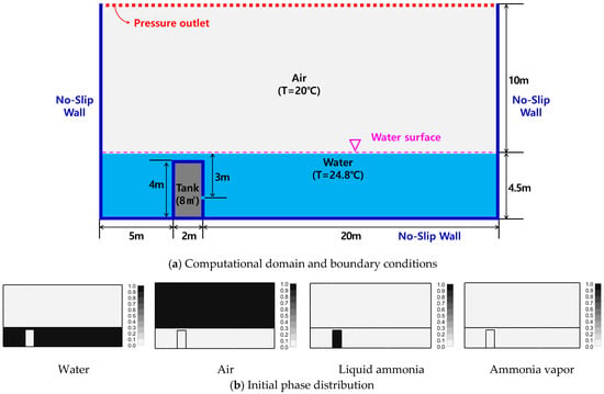
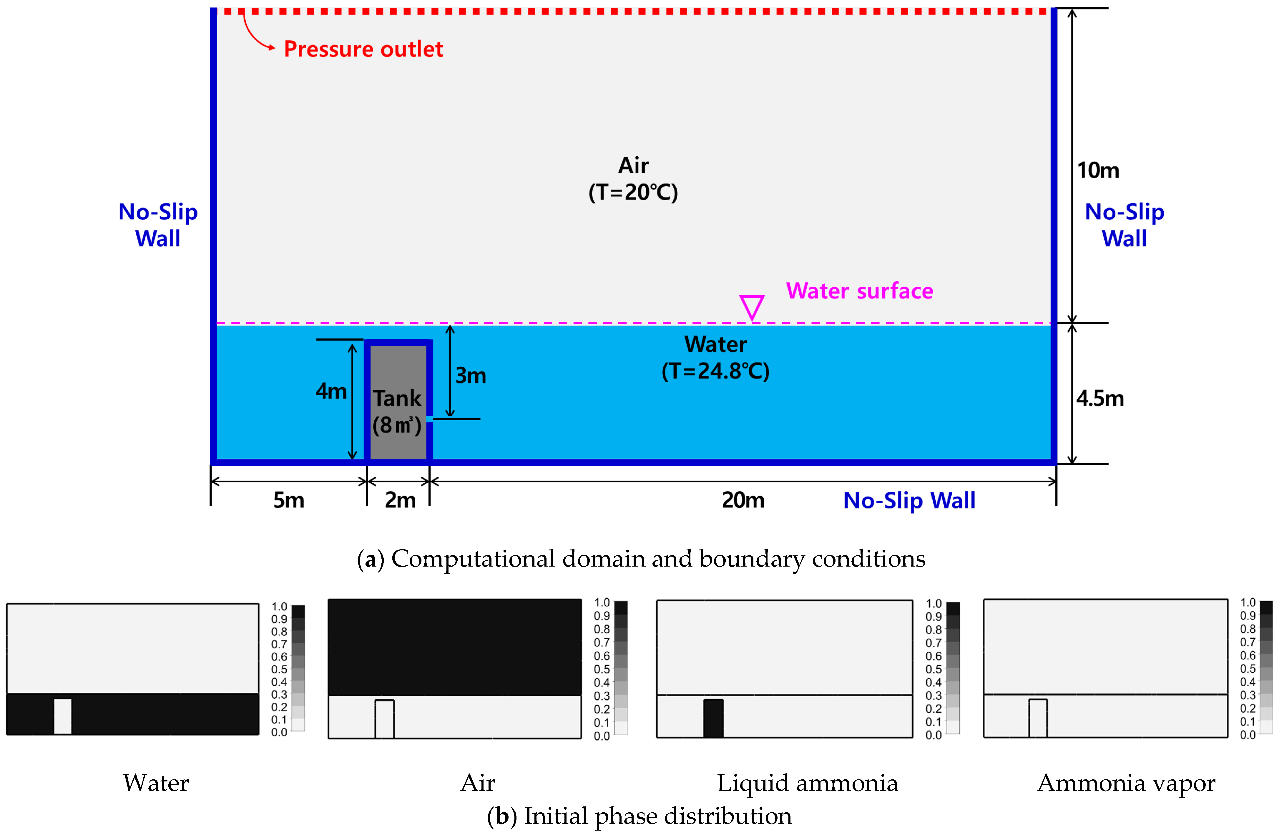
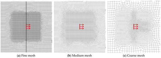
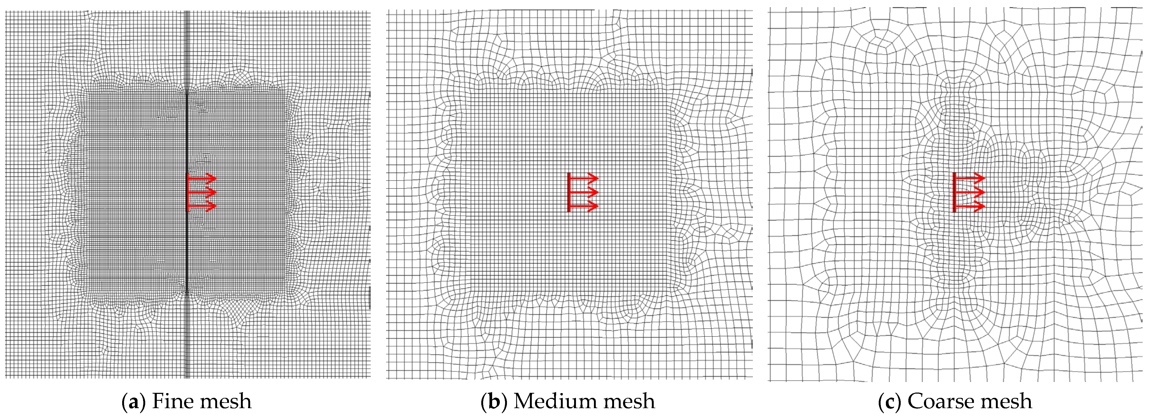
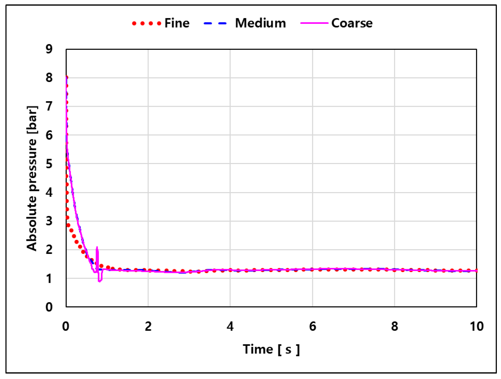
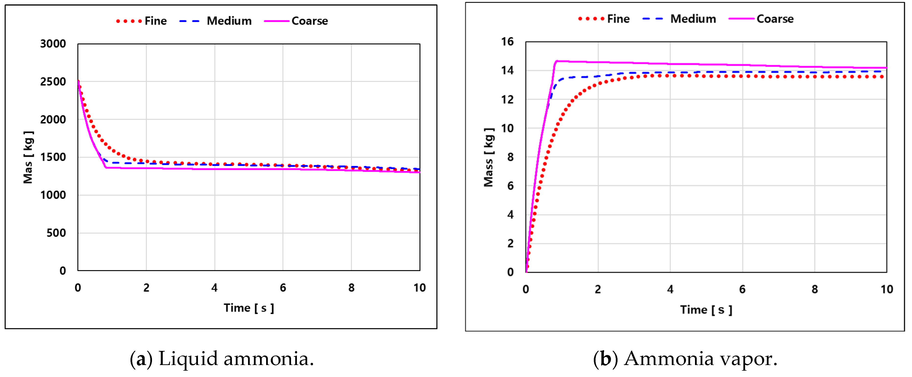
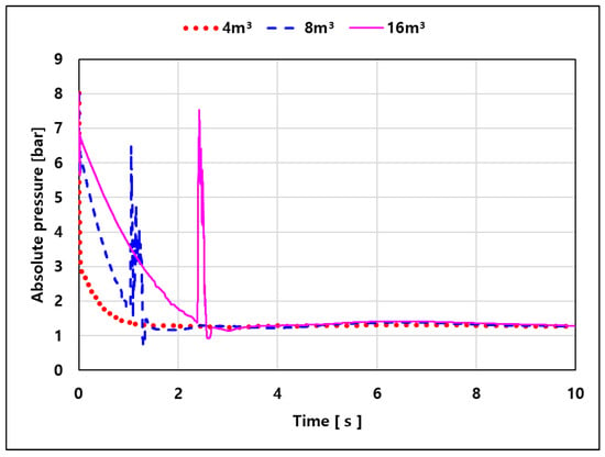
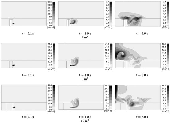
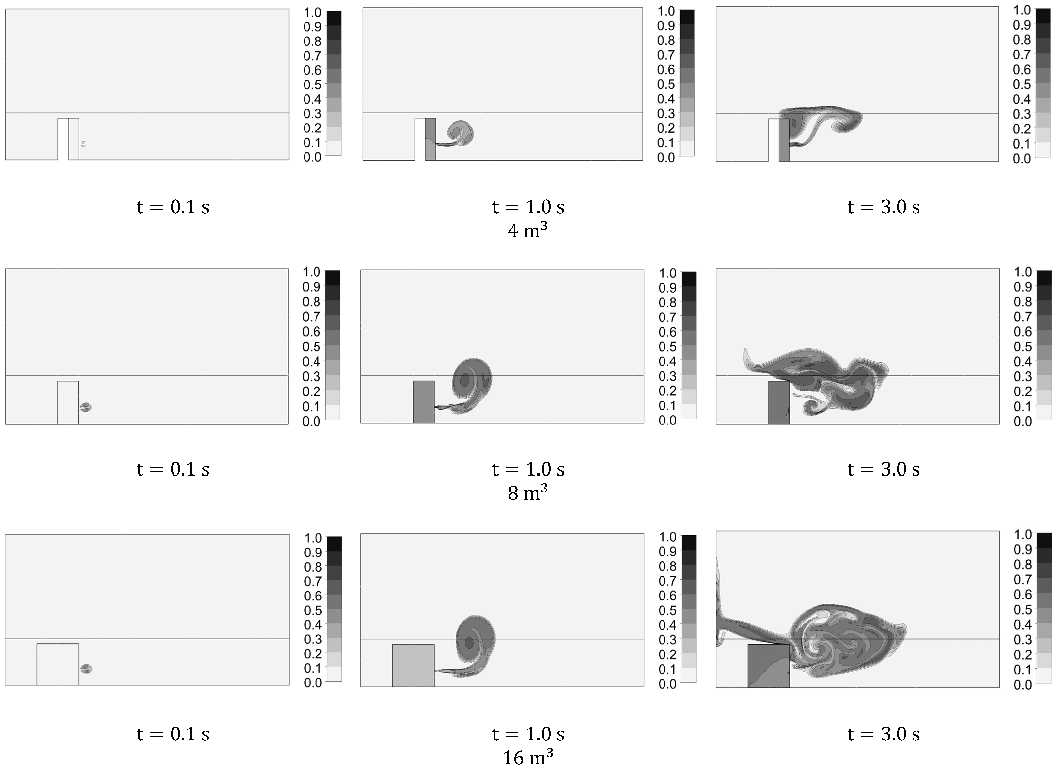
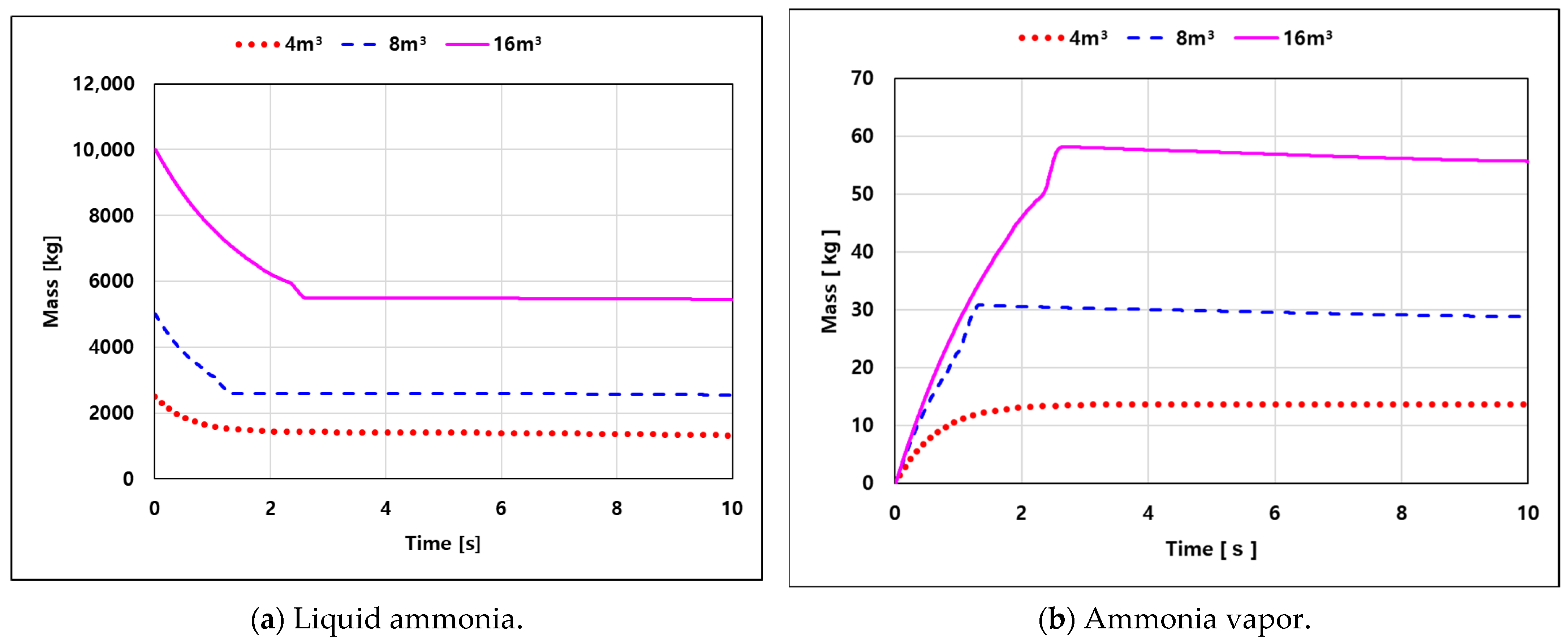
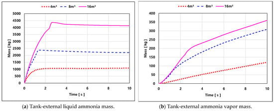
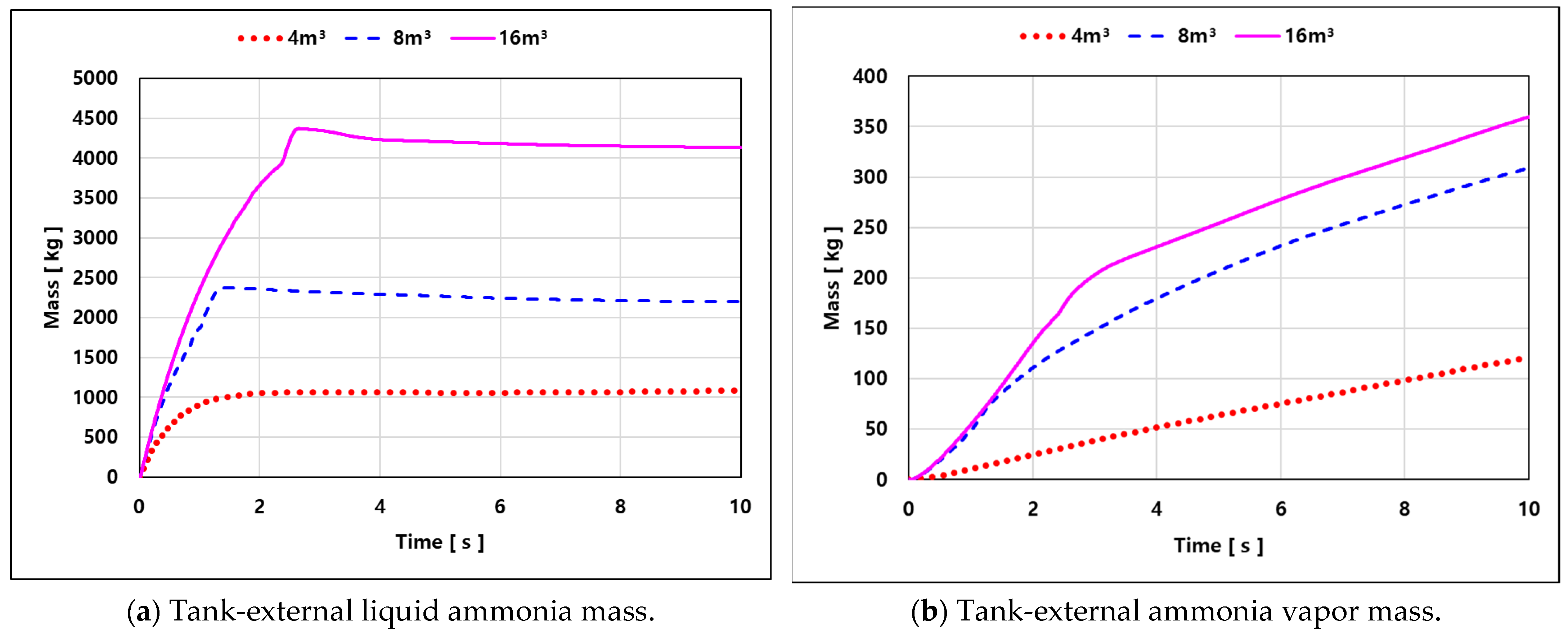
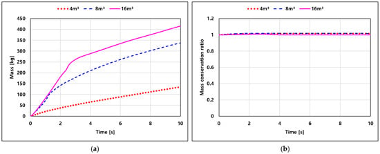
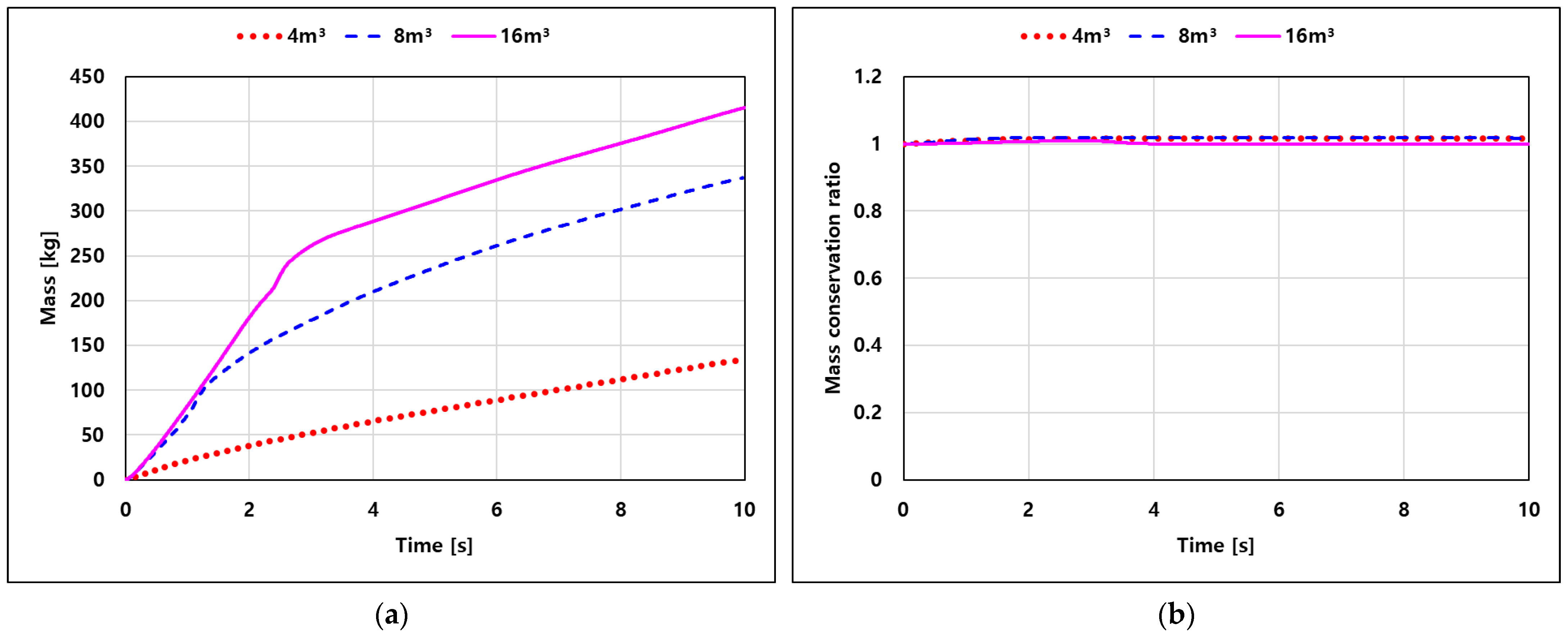

Disclaimer/Publisher’s Note: The statements, opinions and data contained in all publications are solely those of the individual author(s) and contributor(s) and not of MDPI and/or the editor(s). MDPI and/or the editor(s) disclaim responsibility for any injury to people or property resulting from any ideas, methods, instructions or products referred to in the content. |
© 2026 by the authors. Licensee MDPI, Basel, Switzerland. This article is an open access article distributed under the terms and conditions of the Creative Commons Attribution (CC BY) license.