Physics-Informed Neural Networks for Time-Dependent Moderate Reynolds Flow Around a Rotating Cylinder: A Study of Lift, Drag, and Wake Dynamics

Abstract

This study assesses physics-informed neural networks (PINNs) for the unsteady two-dimensional flow past a rotating circular cylinder confined in a channel (blockage ratio 0.2) at Reynolds numbers of 50, 200 and 500. The networks are trained on the non-dimensional Navier–Stokes residuals, the boundary conditions including the rotating wall, and an initial velocity field, using adaptive loss weighting and time marching. A finite-volume reference solver, verified against the Schäfer–Turek benchmark to within 1.2%, is used to quantify the PINN accuracy and to characterise the flow for rotation ratios between $-1$ and 1.5. Rotation produces a Magnus lift that increases almost linearly with the rotation ratio ($\overline{C_l}\approx -3.7\alpha$), reduces the mean drag and leaves the Strouhal number nearly unchanged, while all cases, including the stationary cylinder at $Re=50$, exhibit periodic vortex shedding. The data-free PINN reproduces the wake topology and the sign of the Magnus lift, with relative $L_2$ velocity errors of 14–24%, but underestimates the pressure and the hydrodynamic forces. A systematic ablation shows that sparse velocity data (0.4% of the domain) halve the velocity error, and that a hard rotating-wall constraint with boundary-layer sampling further reduces it to 6% and lowers the lift error to 30% at $Re=50$. The persistent force errors at higher Reynolds numbers identify the representation of the thin rotating boundary layer as the principal limitation of PINNs for this class of flows.

1. Introduction

Numerical simulations have over the last few decades been considered to be one of the most successful methods of solving non-linear Partial Differential Equations (PDEs) in engineering applications. An illustration case is the Navier–Stokes equations being solved using Computational Fluid Dynamics (CFD). Although they are very reliable, such methods can be computationally expensive because of the requirement to produce highly refined and complex computational grids. Not only does this process raise the computational cost but it also demands high expertise and domain-specific knowledge, especially in practice. Over the past few years, the application of modern computational methods to traditional engineering problems has become of interest. One of them is deep learning, which has turned out to be a promising complement due to the development of training algorithms, neural network structures, and greater computing capabilities. Artificial neural networks (ANNs) can effectively approximate complicated relationships between input and output variables using layered transformations. The models are usually trained by optimizing a loss, e.g., the mean squared error between actual data and the predicted output. ANNs can accurately interpolate the data on which they were trained, while extrapolation beyond the training data is still a great challenge [1,2].

In spite of these benefits, there are a number of limitations with deep learning approaches. The fact that it may demand huge amounts of labeled data is one of the major issues and may be quite costly and hard to access in engineering. Moreover, neural networks can be black boxes, so the processes that take place within them can be hard to understand. Purely data-driven approaches are rather data-intensive and do not by themselves respect the underlying physical principles, as emphasized by Iskhakov and Dinh [3]. This weakness highlights the need to incorporate domain knowledge in learning frameworks, as argued by Karniadakis et al. [1]. Machine learning methods have been considered to tackle such difficulties in fluid dynamics problems (Faller and Schreck [4]; Michek et al. [5]), and there has been a shift in focus to hybrid methods that unite data-driven models with physical laws. Physics-Informed Neural Networks (PINNs) [6] have become of great interest in this regard (Ren et al. [7]). PINNs use governing PDEs as part of the training process by including them in the loss. The derivatives needed are derived efficiently using automatic differentiation, as described by Chen et al. [8]. The network is conditioned by reducing the residuals of the governing equations at a set of collocation points, so that the physical constraints are met in the predictions. The loss function may also include initial and boundary conditions and thus ensure that the model produces physically meaningful solutions [9].

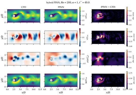
A major benefit of PINNs is that they do not have to rely on labeled data to such an extent. They can often work with little or no training data, and they are based on embedded physical laws. Nonetheless, PINNs are still a rather young field, and their usage in practical engineering matters is still scarce. Systematic comparisons have shown that, for forward problems with a single fixed configuration, PINNs are usually slower and less accurate than classical discretizations [10], and their training suffers from imbalanced loss terms [11,12] and from violations of temporal causality over long time intervals [13]. The majority of the literature has been on enhancing performance in benchmark situations. For example, Sun et al. [14] considered various methods of enforcing the boundary and initial conditions, and Meng et al. [15] suggested training methods based on multiple time windows. On the same note, Wang et al. [11] made general guidelines on how to enhance training efficiency, and adaptive weighting schemes have been proposed to balance the loss terms [12,16]. PINN-based solutions have been suggested in several studies in the context of the Navier–Stokes equations. Xiao et al. [17] came up with a surrogate model for incompressible flows with hard imposed boundary conditions, whereas Jin et al. [18] came up with NSFNet to solve three-dimensional flows in both laminar and turbulent conditions. Rao et al. [19] developed a mixed-form formulation that uses Cauchy stress and stream functions. Moreover, Gao et al. [20] created PhyGeoNet on the basis of convolutional neural networks and Ranade et al. [21] created a discretization-based neural network based on finite volume methods. Raissi et al. [22] inferred hidden velocity and pressure fields of the cylinder wake from flow visualizations, whereas Chuang and Barba [23] reported that a data-free PINN failed to develop vortex shedding behind a stationary cylinder. Recent review studies have comprehensively examined the development, applications, training strategies, and challenges of PINNs for solving partial differential equations [24,25,26,27].

Despite these developments, most existing PINN-based investigations of flow around circular cylinders have primarily focused on stationary cylinders, where the conventional no-slip boundary condition imposes zero velocity at the cylinder surface. In contrast, a rotating cylinder introduces a moving-wall boundary condition with a non-zero tangential surface velocity, ${\mathbf{u}}_w=\mathit{\omega }\times \mathbf{r}$, and its rotational intensity can be characterized by the dimensionless rotation ratio $\alpha =\omega D/\left(2U_{\mathrm{ref}}\right)$. This distinction is physically important because cylinder rotation modifies near-wall momentum transfer, alters flow separation and vortex shedding, produces asymmetric velocity and pressure distributions, and generates lift through the Magnus effect [28,29,30]. Consequently, a PINN for a rotating cylinder must learn the unsteady Navier–Stokes dynamics while simultaneously satisfying the rotation-dependent moving-wall boundary condition, and the Magnus lift, which depends on the surface pressure and shear stress, must be obtained from derivatives of the network outputs. This provides a more challenging flow-learning problem than the conventional stationary-cylinder configuration and motivates the present investigation.

This paper introduces a Physics-Informed Neural Network (PINN) for solving the time-dependent two-dimensional incompressible Navier–Stokes equations governing flow around a rotating circular cylinder at moderate Reynolds numbers. The governing equations are directly incorporated into the loss function of a neural network, so no mesh is needed. The framework is developed to capture the unsteady flow attributes, such as vortex shedding, the growth of the wake, and the separation of the flow, as well as the impact of the cylinder rotation on the lift generated through the Magnus effect. Reynolds numbers of 50, 200 and 500 are simulated and the predicted flow is compared with CFD results. Besides the qualitative flow visualization, there is a quantitative analysis of the drag and lift coefficients, in order to evaluate the accuracy of the method.

• Contribution of this work

We do not propose a new network architecture. To our knowledge, a quantitative assessment of a data-free PINN against a verified CFD solution for the confined flow past a rotating cylinder has not been reported. The contribution of this study is such an assessment, with three parts. (i) Physical: using the verified CFD, we quantify how the rotation ratio and direction ($\alpha =0$, 0.5, 1, 1.5 and $-1$) change the mean and fluctuating forces, the Strouhal number and the wake of a confined cylinder at $Re=50$, 200 and 500. (ii) Computational: we measure where and by how much the PINN deviates from the CFD, using error fields, relative $L_2$ errors and force histories, and we separate the training residuals from the true prediction errors. (iii) Methodological: we document a reproducible PINN set-up with a loss-magnitude-based adaptive weighting, whose effect is quantified against fixed weights over several random seeds.

• Aim of the Study:

The main objective of this research is to design and test a Physics-Informed Neural Network (PINN) which can predict the unsteady incompressible flow around a rotating circular cylinder at moderate Reynolds numbers, and to assess its accuracy and cost against a verified CFD solution.

• Objectives:

• To create a PINN model to solve the time-dependent Navier–Stokes equations without mesh-based discretization.
• To model the flow around a rotating cylinder at Reynolds numbers of 50, 200 and 500.
• To examine important flow characteristics including vortex shedding, formation of the wake, and separation of the flow.
• To determine the effects of cylinder rotation (rotation ratio and direction) on lift, drag and asymmetry of the flow.
• To calculate and compare the drag and lift coefficients with verified CFD results.
• To determine the accuracy, efficiency, and constraints of the PINN framework in unsteady flow simulations.

The proposed PINN framework has potential applications in engineering fields involving unsteady flow around rotating bodies, including flow control by rotating cylinders, offshore structures, particle transport systems and the cooling of rotating electromechanical parts.

• Research Questions:

• Does a PINN framework have the capability to solve the time-dependent Navier–Stokes equations of unsteady flow problems?
• How well does the proposed model capture vortex shedding and the wake?
• How does the rotation of the cylinder affect the lift and drag?
• How accurate are the PINN predictions compared with CFD results?
• What are the computational benefits and difficulties of solving such problems using PINNs?

• Limitations of the Study:

• PINN training is computationally expensive, especially for higher Reynolds numbers and time-dependent simulations; for a single configuration it is more expensive than the CFD solver.
• Accuracy declines with increasing Reynolds number because of thinner shear layers and more complex wake dynamics.
• The analysis is restricted to two-dimensional flow; for $Re\gtrsim 190$ the real cylinder wake becomes three-dimensional [31], so the $Re=500$ case is a two-dimensional model problem.
• The network takes only $(x,y,t)$ as inputs; each $(Re,\alpha )$ requires a separate training, and the PINN is trained on a short time interval starting from a developed CFD state.
• Network architecture, hyperparameters, and the balancing of the loss terms can have a great impact on the results.

2. Materials and Methods

2.1. Navier-Stokes Equations

The flow considered in this study is two-dimensional, unsteady, and incompressible and is governed by the Navier–Stokes equations. These equations describe the velocity and pressure fields as functions of space and time. Here, $u(x,y,t)$ and $v(x,y,t)$ denote the velocity components in the x- and y-directions, respectively, and $p(x,y,t)$ denotes the pressure field. The governing equations comprise the continuity equation and the momentum equations.

The continuity equation, which represents mass conservation for an incompressible fluid, is given by

$${\displaystyle \frac{\partial u}{\partial x}}+{\displaystyle \frac{\partial v}{\partial y}}=0.$$

(1)

The momentum equation in the x-direction is written as

$${\displaystyle \frac{\partial u}{\partial t}}+u{\displaystyle \frac{\partial u}{\partial x}}+v{\displaystyle \frac{\partial u}{\partial y}}=-{\displaystyle \frac{1}{\rho }}{\displaystyle \frac{\partial p}{\partial x}}+\nu \left({\displaystyle \frac{{\partial }^{2}u}{\partial x^2}}+{\displaystyle \frac{{\partial }^{2}u}{\partial y^2}}\right).$$

(2)

Similarly, the momentum equation in the y-direction is given by

$${\displaystyle \frac{\partial v}{\partial t}}+u{\displaystyle \frac{\partial v}{\partial x}}+v{\displaystyle \frac{\partial v}{\partial y}}=-{\displaystyle \frac{1}{\rho }}{\displaystyle \frac{\partial p}{\partial y}}+\nu \left({\displaystyle \frac{{\partial }^{2}v}{\partial x^2}}+{\displaystyle \frac{{\partial }^{2}v}{\partial y^2}}\right).$$

(3)

In these equations, $\rho$ is the fluid density and $\nu$ is the kinematic viscosity. To include the effect of cylinder rotation, a moving boundary condition is applied on the cylinder surface,

$${\mathbf{u}}_w=\mathbf{\omega }\times \mathbf{r},$$

(4)

where $\mathit{\omega }$ is the angular velocity of the cylinder and $\mathbf{r}$ is the position vector from the cylinder centre. For a two-dimensional circular cylinder, this produces a tangential velocity along the surface, leading to asymmetry in the flow and generation of lift.

Reference scales and non-dimensional form. The inflow profile is parabolic (as defined in Section 2.4), so the reference velocity must be stated explicitly. We use the mean inlet velocity $U_{\mathrm{ref}}=\overline{U}=\frac{2}{3}{U}_{\max }$ and the cylinder diameter D as reference scales. The Reynolds number and the rotation ratio are

$$Re={\displaystyle \frac{U_{\mathrm{ref}}D}{\nu }},\alpha ={\displaystyle \frac{\omega D}{2U_{\mathrm{ref}}}},$$

(5)

so that $\alpha$ is the ratio of the surface speed of the cylinder to the reference velocity. With $x^{\ast }=x/D$, $y^{\ast }=y/D$, $t^{\ast }=t{U}_{\mathrm{ref}}/D$, ${\mathbf{u}}^{\ast }=\mathbf{u}/U_{\mathrm{ref}}$ and $p^{\ast }=p/\left(\rho U_{\mathrm{ref}}^2\right)$, Equations (1)–(3) become

$$\begin{array}{cc}\hfill {\displaystyle \frac{\partial u^{\ast }}{\partial x^{\ast }}}+{\displaystyle \frac{\partial v^{\ast }}{\partial y^{\ast }}}& =0,\hfill \end{array}$$

(6)

$$\begin{array}{cc}\hfill {\displaystyle \frac{\partial u^{\ast }}{\partial t^{\ast }}}+u^{\ast }{\displaystyle \frac{\partial u^{\ast }}{\partial x^{\ast }}}+v^{\ast }{\displaystyle \frac{\partial u^{\ast }}{\partial y^{\ast }}}& =-{\displaystyle \frac{\partial p^{\ast }}{\partial x^{\ast }}}+{\displaystyle \frac{1}{Re}}\left({\displaystyle \frac{{\partial }^2{u}^{\ast }}{\partial x^{\ast 2}}}+{\displaystyle \frac{{\partial }^2{u}^{\ast }}{\partial y^{\ast 2}}}\right),\hfill \end{array}$$

(7)

$$\begin{array}{cc}\hfill {\displaystyle \frac{\partial v^{\ast }}{\partial t^{\ast }}}+u^{\ast }{\displaystyle \frac{\partial v^{\ast }}{\partial x^{\ast }}}+v^{\ast }{\displaystyle \frac{\partial v^{\ast }}{\partial y^{\ast }}}& =-{\displaystyle \frac{\partial p^{\ast }}{\partial y^{\ast }}}+{\displaystyle \frac{1}{Re}}\left({\displaystyle \frac{{\partial }^2{v}^{\ast }}{\partial x^{\ast 2}}}+{\displaystyle \frac{{\partial }^2{v}^{\ast }}{\partial y^{\ast 2}}}\right).\hfill \end{array}$$

(8)

The only physical parameters are therefore $Re$, which enters as the coefficient $1/Re$ of the viscous term, and $\alpha$, which enters through the moving-wall condition (dimensionless surface speed $\alpha$). Equations (6)–(8) are the equations solved by both the PINN and the CFD code. In each simulation, $Re$ and $\alpha$ are fixed constants (constant viscosity), and every $(Re,\alpha )$ pair is a separate simulation. All results below are reported in these non-dimensional variables, and the asterisks are dropped where no confusion arises.

Here, the unsteady flow behavior including the wake and vortex shedding are studied in the cases of $Re=50$, 200, and 500. The baseline rotation ratio is $\alpha =1$. To isolate the effect of rotation, additional cases with $\alpha =0$ (stationary reference), $0.5$ and $1.5$ were computed, together with $\alpha =-1$ (clockwise rotation) at every Reynolds number (Section 4.6).

2.2. Automatic Differentiation

This study uses automatic differentiation (AD) to compute the spatial and temporal derivatives required by the Navier–Stokes equations. It offers a precise and effective approach to computing derivatives of the neural network outputs with regard to the input variables. The PINN model allows the velocity and pressure fields to be modeled by a neural network as functions of the input variables $(x,y,t)$. Because the neural network is a series of differentiable functions, all the derivatives needed can be obtained exactly by Automatic Differentiation [8]. Using the non-dimensional equations, the continuity and momentum residuals are

$$\begin{array}{cc}\hfill R_{\mathrm{mass}}& =u_x+v_y,\hfill \\ \hfill R_x& =u_t+u{u}_x+v{u}_y+p_x-\frac{1}{Re}\left(u_{xx}+u_{yy}\right),\hfill \\ \hfill R_y& =v_t+u{v}_x+v{v}_y+p_y-\frac{1}{Re}\left(v_{xx}+v_{yy}\right),\hfill \end{array}$$

(9)

where subscripts denote partial derivatives obtained by AD. AD enables such derivatives to be calculated without discretization error, in contrast to the conventional CFD techniques, where derivatives depend on mesh resolution and discretization schemes. This is especially significant in viscous flow problems, in which second-order derivatives are needed, and for the force calculation, which requires velocity gradients on the cylinder surface (Section 2.5).

2.3. Physics-Informed Neural Network (PINN) Framework

In this work, the unsteady incompressible Navier-Stokes equations are solved using a Physics-Informed Neural Network (PINN). In order to ensure that the predicted solution satisfies the governing equations, PINNs blend neural networks with physical laws [1,6].

Network. A fully connected feed-forward network approximates the flow variables,

$$\left(u,v,p\right)(x,y,t)\approx {\mathcal{N}}_{\theta }(x,y,t)={\mathbf{W}}_9\sigma \left({\mathbf{W}}_8\cdots \sigma \left({\mathbf{W}}_1\widehat{\mathbf{z}}+{\mathbf{b}}_1\right)\cdots +{\mathbf{b}}_8\right)+{\mathbf{b}}_9,$$

(10)

where $\widehat{\mathbf{z}}$ is the input $(x,y,t)$ linearly scaled to $[-1,1]$, $\sigma =\tanh$, and the eight hidden layers have 64 neurons each. The network has 3 inputs, 3 outputs and 29,571 trainable parameters $\theta =\{{\mathbf{W}}_k,{\mathbf{b}}_k\}$. Throughout the paper, ${\mathcal{N}}_{\theta }$ denotes this specific network. Weights are initialised with the Xavier-normal scheme and biases with zeros.

Loss function. The loss is the weighted sum of four mean-squared terms,

$$\begin{array}{cc}\hfill \mathcal{L}\left(\theta \right)& ={\lambda }_f{\mathcal{L}}_{\mathrm{PDE}}+{\lambda }_b{\mathcal{L}}_{\mathrm{BC}}+{\lambda }_s{\mathcal{L}}_{\mathrm{wall}}+{\lambda }_0{\mathcal{L}}_{\mathrm{IC}},\hfill \\ \hfill {\mathcal{L}}_{\mathrm{PDE}}& ={\displaystyle \frac{1}{N_f}}{\displaystyle \sum _{i=1}^{N_f}}{\left(R_{\mathrm{mass}}^2+R_x^2+R_y^2\right)}_i,{\mathcal{L}}_{\mathrm{wall}}={\displaystyle \frac{1}{N_s}}{\displaystyle \sum _{i=1}^{N_s}}\parallel {\mathbf{u}}_{\theta }-{\mathbf{u}}_w{\parallel }_i^2,\hfill \\ \hfill {\mathcal{L}}_{\mathrm{BC}}& ={\displaystyle \frac{1}{N_b}}{\displaystyle \sum _{i=1}^{N_b}}\parallel \mathcal{B}\left[{\mathcal{N}}_{\theta }\right]-g{\parallel }_i^2,{\mathcal{L}}_{\mathrm{IC}}={\displaystyle \frac{1}{N_0}}{\displaystyle \sum _{i=1}^{N_0}}\parallel {\mathbf{u}}_{\theta }(x_i,y_i,t_0)-{\mathbf{u}}_0(x_i,y_i){\parallel }^2,\hfill \end{array}$$

(11)

where $\mathcal{B}$ collects the inlet, channel-wall and outlet conditions of Section 2.4 (including the convective outflow condition), ${\mathbf{u}}_w$ is the rotating-wall velocity and ${\mathbf{u}}_0$ the initial velocity field. The weights ${\lambda }_k$ act on the loss terms.

Adaptive loss weighting. With equal weights, the four loss terms decrease at very different rates, and the gradient of the PDE term dominates the boundary terms [12]. The weights are therefore updated during the Adam stage from the relative magnitude of the (detached) loss terms. Every $N_u=100$ iterations,

$${\widehat{\lambda }}_k={\displaystyle \frac{{\mathcal{L}}_k}{\frac{1}{4}{\sum }_j{\mathcal{L}}_j}},{\lambda }_k\leftarrow \mathrm{clip}\left((1-\beta ){\lambda }_k+\beta {\widehat{\lambda }}_k,0.1,100\right),k\in \{f,b,s,0\},$$

(12)

with $\beta =0.1$ and ${\lambda }_k=1$ initially. A term whose loss is larger than the average receives a larger weight. The moving average and the clipping prevent abrupt changes of the loss landscape, and the weights are frozen during the L-BFGS stage. The cost is a few scalar operations per update. This rule is a loss-magnitude variant of the learning-rate annealing of Wang et al. [12]. It is compared with fixed weights (${\lambda }_k\equiv 1$) in Section 4.7.

Time marching and initial condition. A single network trained from rest over a long time interval tends to converge to a nearly steady solution and does not develop vortex shedding [13,23]. We therefore use the PINN as a forward solver over a time interval in the developed flow, divided into consecutive windows [15]. The first window starts at $t_0^{\ast }=47$, at which the flow has reached its periodic (or steady) state. Its initial condition ${\mathbf{u}}_0$ is the CFD velocity field at $t_0^{\ast }$, evaluated at the $N_0$ initial points. Each following window starts from the PINN’s own prediction at the end of the previous window, and its network is initialised with the weights of the previous one. No CFD data other than this single initial velocity field enter the training: the pressure and the whole evolution over the windows are obtained from the physics alone. We use two windows of length $\Delta t^{\ast }=1$.

Improved (hybrid) PINN. To identify which ingredients limit the accuracy, a second, improved variant was trained with the same network and time windows, with two modifications. (i) Near-wall sampling: a quarter of the interior collocation points is placed in the annulus $R\le r\le R+0.5D$, with a density that increases towards the wall, to resolve the thin shear layers created by the moving wall. (ii) Sparse velocity data: 400 randomly chosen CFD velocity samples $(u,v)$ per stored instant within each window, about 0.4% of the grid cells, are added through a data loss

$${\mathcal{L}}_{\mathrm{data}}={\displaystyle \frac{1}{N_d}}{\displaystyle \sum _{i=1}^{N_d}}\parallel {\mathbf{u}}_{\theta }(x_i,y_i,t_i)-{\mathbf{u}}_i^{\mathrm{CFD}}{\parallel }^2,$$

(13)

which enters Equation (11) with its own adaptive weight. The Adam stage was extended to 10,000 iterations. The pressure and the forces are not used in training, so they remain an independent test of the physics learned by the network. This variant is therefore a data-assisted PINN [22], and we report it separately from the data-free PINN. A third variant (hybrid + hard wall) additionally builds the rotating-wall condition into the network output (Section 4.5) and concentrates 35% of the interior points within $0.5D$ of the wall.

Total Optimization Problem. The training of the PINN is formulated as an optimization problem:

$${\theta }^{\ast }=\arg \underset{\theta }{\min }\mathcal{L}\left(\theta \right),$$

(14)

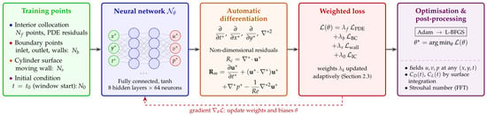
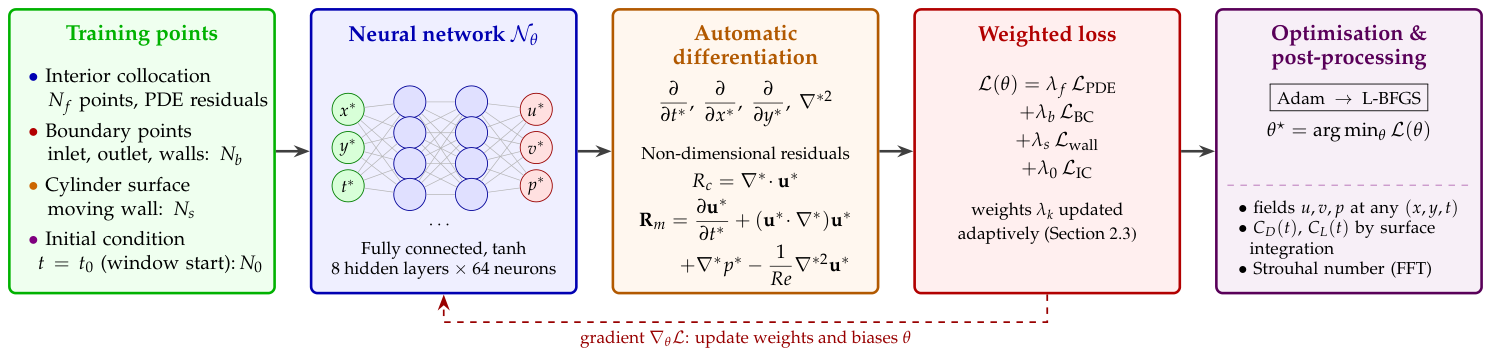
where ${\theta }^{\ast }$ represents the optimal network parameters. The complete training and post-processing sequence is shown in Figure 1.

Figure 1. Proposed PINNs framework for solving flow around a rotating circular cylinder. Training points are passed through the network ${\mathcal{N}}_{\theta }$; the non-dimensional Navier–Stokes residuals are formed by automatic differentiation and combined with the boundary, moving-wall and initial-condition losses using adaptive weights ${\lambda }_k$; the network is optimised with Adam followed by L-BFGS. Arrows indicate the forward processing direction, coloured boxes distinguish the training stages and the ellipsis represents the intervening hidden network layers.

2.4. Investigated Domain

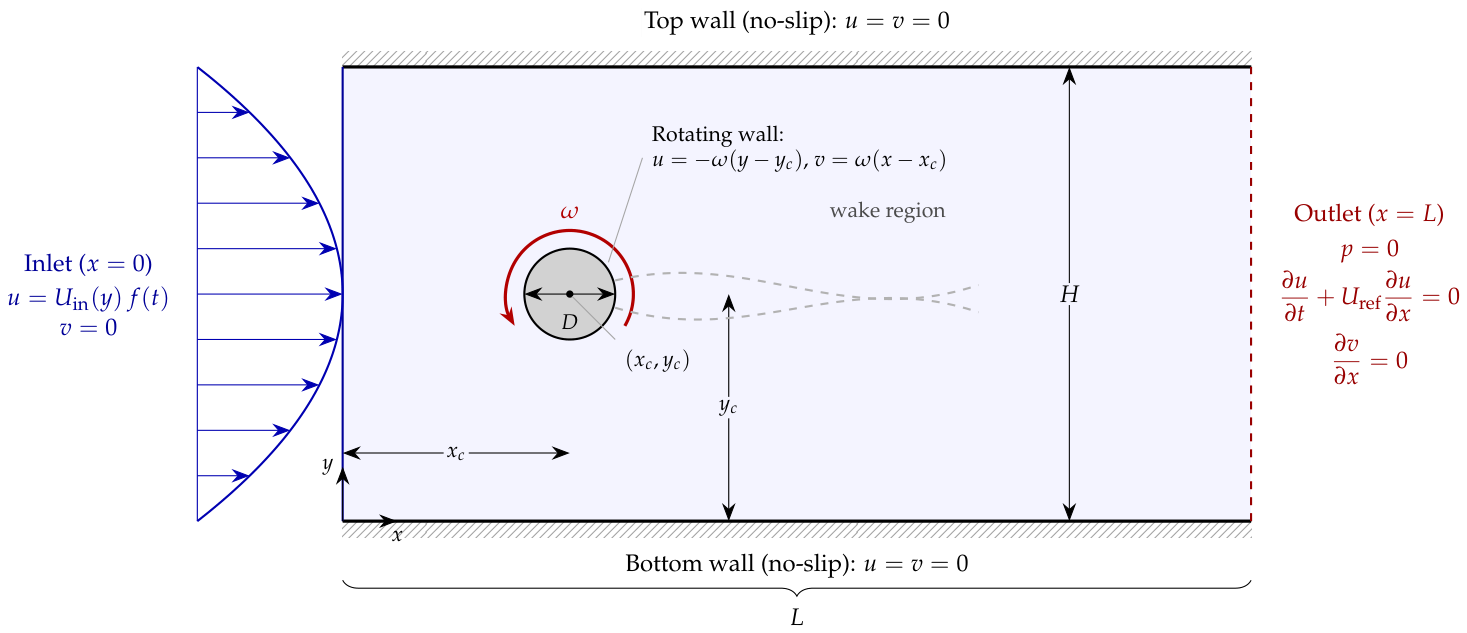
The computational domain considered in this study is a two-dimensional rectangular channel containing a circular cylinder placed inside the flow field. Let the domain be defined as $\mathsf{\Omega }=[0,L]\times [0,H]$, where L is the length and H is the height of the channel. A circular cylinder of diameter D is located at $(x_c,y_c)$. The dimensions are $L=12.5D$, $H=5D$ (blockage ratio $D/H=0.2$), $x_c=2.5D$ and $y_c=H/2$; all parameters are listed in Table 1.

Table 1. Geometric and physical parameters (non-dimensional, $\rho =1$, $D=1$, $U_{\mathrm{ref}}=1$).

Parameter	Symbol	Value
Channel length and height	L, H	12.5, 5
Cylinder diameter/centre	D/$(x_c,y_c)$	1/(2.5, 2.5)
Blockage ratio	$D/H$	0.2
Maximum/mean (reference) inlet velocity	$U_{\max }$/$U_{\mathrm{ref}}$	1.5/1.0
Kinematic viscosity	$\nu =1/Re$	$2\times {10}^{-2}$, $5\times {10}^{-3}$, $2\times {10}^{-3}$
Reynolds number	$Re$	50, 200, 500
Rotation ratio	$\alpha$	1 (baseline); 0, 0.5, 1.5, $-1$
Angular velocity	$\omega =2\alpha$	2 for $\alpha =1$
Ramp time	$t_r$	5
Simulated time (CFD)	$[0,T]$	$[0,50]$
Statistics window (CFD)	$[t_s,T]$	$[30,50]$
PINN time windows	$[t_0,t_0+2]$	$[47,48]$, $[48,49]$

At the inlet boundary ($x=0$), a parabolic velocity profile is prescribed and ramped smoothly in time,

$$u(0,y,t)={\displaystyle \frac{4U_{\max }y(H-y)}{H^2}}f\left(t\right),v(0,y,t)=0,f\left(t\right)=\left\{\begin{array}{cc}{\sin }^2\left({\displaystyle \frac{\pi t}{2t_r}}\right),\hfill & t<t_r,\hfill \\ 1,\hfill & t\ge t_r,\hfill \end{array}\right.$$

(15)

which represents a fully developed laminar inflow condition. At the outlet boundary ($x=L$), a zero-pressure condition $p=0$ is applied, together with a convective condition $\partial u/\partial t+U_{\mathrm{ref}}\partial u/\partial x=0$ and $\partial v/\partial x=0$, which allow vortices to leave the domain with minimal artificial reflection. No-slip boundary conditions $u=v=0$ are imposed on the top and bottom walls of the channel. On the cylinder surface, the rigid-body rotation gives

$$u=-\omega f\left(t\right)(y-y_c),v=\omega f\left(t\right)(x-x_c),$$

(16)

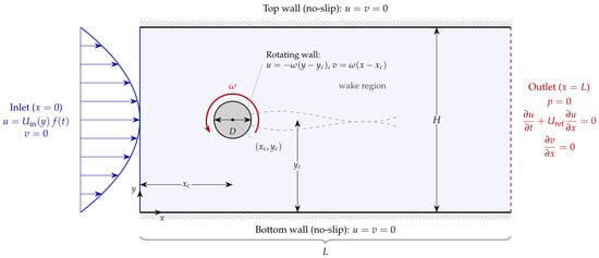
a purely tangential surface velocity of magnitude $\omega D/2=\alpha U_{\mathrm{ref}}$; $\alpha >0$ is counter-clockwise and $\alpha <0$ clockwise rotation. The initial condition is a fluid at rest, $u=v=0$, $p=0$. Because $f\left(0\right)=f^{\prime }\left(0\right)=0$, the boundary velocities vanish at $t=0$, so the initial and boundary conditions are compatible and no discontinuity occurs at the initial instant. The ramp time is $t_r^{\ast }=5$, much shorter than the time before statistics are collected. For $\alpha =0$, the configuration is exactly symmetric about the channel centreline. A symmetric numerical solution then remains symmetric even when it is unstable, so a weak transient rotation pulse (peak rotation ratio $0.25$, $\omega \left(t\right)\propto \sin (\pi t/t_r)$ for $t<t_r$, zero afterwards) is applied during the ramp to seed the physical instability. It has no influence on the developed flow. Figure 2 illustrates the computational domain and boundary conditions.

Figure 2. Computational domain of the benchmark case, with the boundary conditions. Dimensions are given in Table 1. The blue inlet arrows indicate the incoming parabolic flow; the curved arrow indicates cylinder rotation; the red dashed outlet line identifies the downstream boundary, and the shaded region indicates the channel wake.

Sampling of the training points. In each time window, the training points are drawn at random (uniformly in time over the window):

• $N_f=\mathrm{20,000}$ interior collocation points in $\mathsf{\Omega }\setminus \left\{\mathrm{cylinder}\right\}$, half of them uniformly over the channel and half inside a refinement box $[x_c-1.5D,x_c+5D]\times [y_c-1.5D,y_c+1.5D]$ around the cylinder and the near wake;
• $N_b$ = 4000 points on the inlet, outlet and channel walls, 1000 on each;
• $N_s=3000$ points on the cylinder surface, uniform in the polar angle;
• $N_0=\mathrm{10,000}$ initial-condition points at $t=t_0$, distributed like the interior points.

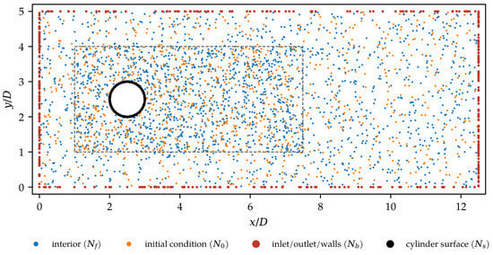
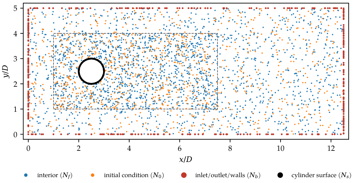
The initial-condition points are distributed across the channel to capture the developed vortex street. Figure 3 shows a subset of the points of one window.

Figure 3. Samples within the domain (10% of the points of one window, drawn by the training code): interior collocation points (blue), boundary points (red), cylinder-surface points (black) and initial-condition points (orange). The dashed rectangular outline marks the enhanced-sampling box around the cylinder and near wake.

2.5. Drag and Lift Force Coefficients

The drag and lift forces on the cylinder are essential measures of the performance of the proposed PINN model. The drag force acts in the flow direction and the lift force perpendicular to it. The non-dimensional coefficients are

$$C_d={\displaystyle \frac{2F_d}{\rho U_{\mathrm{ref}}^{2}D}},C_l={\displaystyle \frac{2F_l}{\rho U_{\mathrm{ref}}^{2}D}},$$

(17)

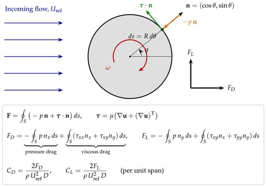
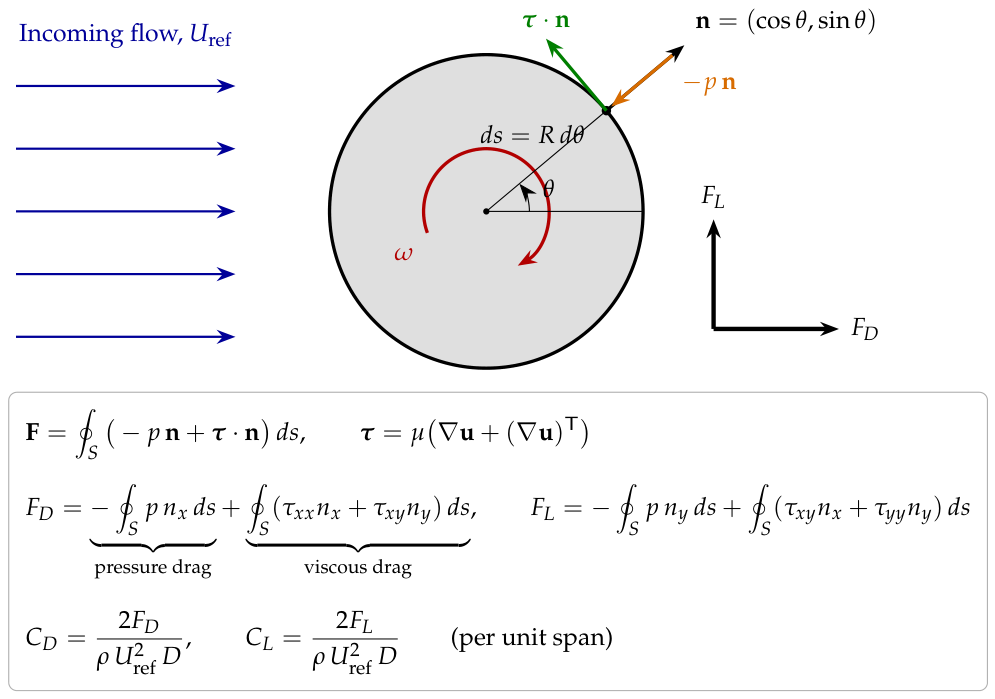
with forces per unit span. The overall drag force is composed of two parts, pressure drag and viscous drag, $F_d=F_p+F_v$. The pressure drag is caused by the pressure difference between the front and rear of the cylinder, while the viscous drag is due to shear stress along the cylinder surface (Figure 4):

$$\begin{array}{cccc}\hfill F_p& =-{\oint }_{S}p{n}_{x}ds,\hfill & \hfill F_v& ={\oint }_S\left({\tau }_{xx}{n}_x+{\tau }_{xy}{n}_y\right)ds,\hfill \\ \hfill {\tau }_{xx}& =2\mu {\displaystyle \frac{\partial u}{\partial x}},\hfill & \hfill {\tau }_{xy}& =\mu \left({\displaystyle \frac{\partial u}{\partial y}}+{\displaystyle \frac{\partial v}{\partial x}}\right),\hfill \end{array}$$

(18)

and the lift follows analogously from the y-components. For a circular cylinder of radius r, $n_x=\cos \theta$, $n_y=\sin \theta$ and $ds=rd\theta$, and the integrals are approximated with the trapezoidal rule on equally spaced surface points:

$$F_p\approx -{\displaystyle \sum _{i=1}^N}{p}_i\cos {\theta }_{i}r\Delta \theta ,F_v\approx {\displaystyle \sum _{i=1}^N}\left[2\mu {\displaystyle \frac{\partial u}{\partial x}}{|}_i\cos {\theta }_i+\mu {\left({\displaystyle \frac{\partial u}{\partial y}}+{\displaystyle \frac{\partial v}{\partial x}}\right)}_i\sin {\theta }_i\right]r\Delta \theta .$$

(19)

In the PINN framework, $p_i$ and the velocity gradients are obtained directly from the network and by AD at $N=256$ surface points. In the CFD, the total force is obtained from a control-volume momentum balance on a $2D\times 2D$ box around the cylinder, and the pressure drag from the surface pressure, which is extrapolated to the wall from two rings of points at $1.5h$ and $2.5h$. The viscous drag is the difference of the two. The pressure drag becomes more significant at higher Reynolds numbers, whereas the viscous drag is relatively more important at lower Reynolds numbers.

Figure 4. Illustration of the drag and lift force calculation: pressure ($-p\mathbf{n}$) and viscous ($\mathit{\tau }·\mathbf{n}$) surface tractions on the rotating cylinder.

2.6. CFD Validation

The reference solutions are computed with an in-house finite-volume solver written in Python 3 (NumPy/SciPy). The solver uses the same geometry, governing equations, ramp and boundary conditions as the PINN. Its numerical method is as follows:

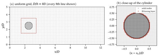
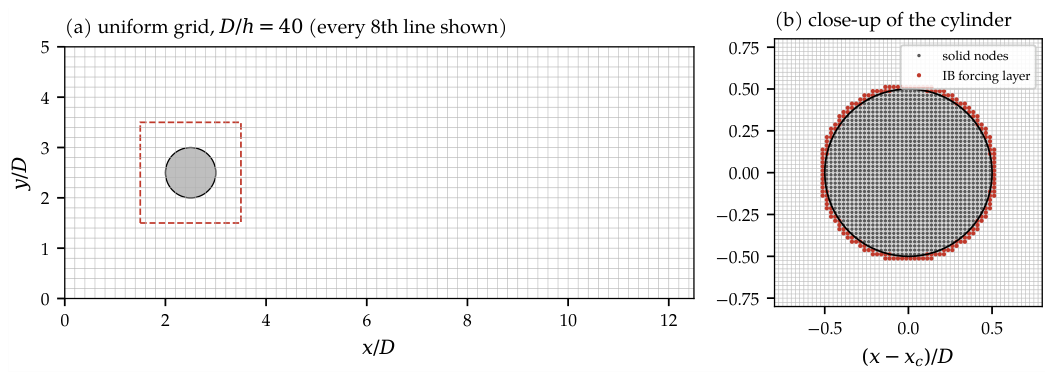
• Grid: uniform staggered (MAC) Cartesian grid with $h=D/40$, i.e., $500\times 200=\mathrm{100,000}$ cells (Figure 5).
• Cylinder: sharp-interface direct-forcing immersed boundary method [32]. Velocity nodes inside the cylinder are set to the rigid-body rotation. On the first layer of fluid nodes, the velocity is interpolated linearly along the wall normal between the wall velocity of Equation (16) and the flow at a distance h further out.
• Spatial discretisation: conservative finite-volume form. Convective fluxes use QUICK interpolation [33] of the transported velocity, and diffusive fluxes second-order central differences.
• Pressure–velocity coupling: fractional-step projection method [34]. The pressure Poisson equation (Neumann conditions at the inlet and walls, $p=0$ at the outlet) is solved to machine precision by fast cosine transforms. The maximum velocity divergence after projection is below ${10}^{-12}$ in all runs.
• Time integration: second-order Adams–Bashforth for convection and diffusion, with a constant time step from the Courant condition $\mathrm{CFL}=0.3$ and the viscous stability limit ($\Delta t^{\ast }=2.0\times {10}^{-3}$–$3.75\times {10}^{-3}$).
• Run length: $t^{\ast }\in [0,50]$. Statistics are collected over $t^{\ast }\in [30,50]$, which covers six or more shedding cycles. Convergence to the periodic state was checked from the cycle-to-cycle variation of the lift (see Section 4.4).
• Hardware: one core of an x86-64 Linux server per run.

Figure 5. Computational grid of the benchmark case in CFD: (a) uniform Cartesian grid ($D/h=40$; every eighth grid line drawn) with the control volume used for the forces (dashed); (b) close-up of the cylinder with the solid nodes and the immersed-boundary forcing layer.

2.7. PINN Architecture and Training Setup

Table 2 summarises the PINN set-up. Training of each window consists of three stages. First, the network is fitted to the initial velocity field for 2000 Adam iterations (first window only; later windows start from the previous network). Second, the full loss of Equation (11) is minimised with Adam for 6000 iterations. Each iteration uses a mini-batch of 1024 interior points and 256 points of each boundary and initial set, and the learning rate starts at ${10}^{-3}$ and decays by a factor 0.7 every 1000 iterations. Third, the loss is minimised with full-batch L-BFGS [35] for 100 iterations (strong-Wolfe line search, 8000 interior points). All trainings ran on the CPU of a desktop computer (Intel Core processor, 12 logical cores, 8 GB RAM, no GPU), with 4 threads per training and three trainings in parallel.

Table 2. PINN architecture and training parameters.

Item	Setting
Inputs/outputs	$(x,y,t)$ scaled to $[-1,1]$/$(u,v,p)$, non-dimensional
Hidden layers × neurons	$8\times 64$, fully connected, tanh
Initialisation/parameters	Xavier-normal/29,571
Training points per window	$N_f=\mathrm{20,000}$, $N_b=4000$, $N_s=3000$, $N_0=\mathrm{10,000}$
Time windows	2 windows of $\Delta t^{\ast }=1$ starting at $t_0^{\ast }=47$
Stage 0 (first window)	Adam, fit of the initial velocity, 2000 iterations
Stage 1	Adam, ${\eta }_0={10}^{-3}$, $\times 0.7$ every 1000 it., 6000 iterations, batch 1024
Stage 2	L-BFGS, 100 iterations, 8000 interior points
Loss weights	adaptive, Equation (12) (or fixed ${\lambda }_k=1$ for comparison)
Software/hardware	PyTorch 2.14 (CPU)/Intel Core CPU, 4 threads

2.8. Error Metrics

Two distinct categories of quantities are reported separately. The training residuals (${\mathcal{L}}_{\mathrm{PDE}}$, ${\mathcal{L}}_{\mathrm{BC}}$, ${\mathcal{L}}_{\mathrm{wall}}$, ${\mathcal{L}}_{\mathrm{IC}}$) measure how well the network satisfies the equations at the collocation points. The prediction errors compare the PINN with the independent CFD solution at all $N_e\approx \mathrm{98,700}$ CFD cell centres outside the cylinder. For $q\in \{u,v,p,|\mathbf{u}\left|\right\}$,

$$e_q(\mathbf{x},t)=|q^{\mathrm{PINN}}-q^{\mathrm{CFD}}|,{\epsilon }_q\left(t\right)={\displaystyle \frac{{\left({\sum }_{i=1}^{N_e}{(q_i^{\mathrm{PINN}}-q_i^{\mathrm{CFD}})}^2\right)}^{1/2}}{{\left({\sum }_{i=1}^{N_e}{\left(q_i^{\mathrm{CFD}}\right)}^2\right)}^{1/2}}}.$$

(20)

The variables are non-dimensional. Because the pressure is defined only up to a constant, its spatial mean is subtracted from both fields before comparison. ${\epsilon }_q$ is evaluated at the CFD output instants within the PINN windows (every $0.2$ time units), and ${\overline{\epsilon }}_q$ denotes its average over the two windows. The force coefficients of the CFD are characterised by their mean $\overline{C}$ and amplitude $\widehat{C}=\frac{1}{2}(C_{\max }-C_{\min })$ over the statistics window. The shedding frequency f is obtained from the zero crossings of $C_l\left(t\right)-\overline{C_l}$, and the Strouhal number is $St=fD/U_{\mathrm{ref}}$.

• Grid and time-step independence

Grid independence was assessed at the most demanding case, $Re=500$ and $\alpha =1$, on three uniform grids with a constant refinement ratio $r=1.4$ ($D/h=28$, 40 and 56). Time-step independence was assessed on the medium grid by halving the time step. The monitored quantities were the mean drag and lift, the lift amplitude, the Strouhal number, and the peak time-mean vorticity at $0.1D$ from the wall, which measures the near-wall velocity gradient. Table 3 lists these quantities together with the grid convergence index (GCI) of Roache [36]. Between the medium and fine grids, the mean drag changes by 0.9%, the mean lift by 0.5%, the lift amplitude by 3.2% and the Strouhal number by 0.2%. Halving the time step changes these quantities by at most 3.6%. The medium grid ($D/h=40$) with $\mathrm{CFL}=0.3$ is therefore used for all results.

Table 3. Grid independence study and time-step sensitivity at $Re=500$, $\alpha =1$. ${\omega }_{\max }$ is the peak time-mean vorticity $|{\omega }_z|D/U_{\mathrm{ref}}$ at $r=0.6D$; GCI is the grid convergence index of the medium-grid value ($r=1.4$, safety factor 1.25).

Grid/Time Step	Cells	$\mathsf{\Delta }{\mathit{t}}^{\ast }$	$\overline{{\mathit{C}}_{\mathit{d}}}$	$\overline{{\mathit{C}}_{\mathit{l}}}$	${\widehat{\mathit{C}}}_{\mathit{l}}$	$\mathit{St}$	${\mathit{\omega }}_{\max }$
Coarse, $D/h=28$	49,000	3.57 $\times {10}^{-3}$	2.8808	−3.7986	2.3984	0.3398	19.82
Medium, $D/h=40$	100,000	2.50 $\times {10}^{-3}$	2.9725	−3.7235	2.6406	0.3464	21.15
Fine, $D/h=56$	196,000	1.79 $\times {10}^{-3}$	2.9460	−3.7059	2.7266	0.3457	22.03
GCImedium (%)	–	–	1.17	0.62	4.11	0.26	9.50
Medium, $\Delta t/2$	100,000	1.25 $\times {10}^{-3}$	2.9031	−3.8559	2.5808	0.3471	21.08

3. CFD Validation and Benchmark Verification

The finite-volume solver is verified against the established confined-cylinder benchmark of Schäfer and Turek [37], which considers channel flow with a parabolic inlet velocity profile. Unlike the stationary-cylinder flow in an unconfined domain discussed by Williamson [31], the present study investigates a rotating cylinder within a confined channel. Therefore, direct quantitative comparison with unconfined stationary-cylinder results is not appropriate. The benchmark blockage ratio ($D/H=0.24$) is of the same order as that of the present configuration. Case 2D-1 is steady ($Re=20$), and case 2D-2 is periodic ($Re=100$, both based on the mean inflow velocity). The benchmark geometry ($L=2.2$, $H=0.41$, $D=0.1$, centre at $(0.2,0.2)$) was computed with the same solver and the same resolution ($D/h=40$) as the present study. Table 4 shows that all quantities agree with the benchmark bounds to within 1.2%: the drag coefficients lie 0.2% and 1.2% above the upper bound, the maximum lift lies 0.6% below the lower bound, and the Strouhal number and steady lift lie within their bounds. The moving-wall implementation was further checked by computing the case with the direction of rotation reversed ($\alpha =-1$). For this case the flow must be the mirror image of the $\alpha =1$ flow about the channel centreline. Indeed, the computed mean drag, lift amplitude and Strouhal number agree to three significant digits or better, and the mean lift changes sign (see Section 4.6).

Table 4. Verification of the CFD solver against the confined-cylinder benchmark of Schäfer and Turek [37] (reference values: bounds of the benchmark).

Case	Quantity	Present CFD	Benchmark [37]
2D-1, $Re=20$ (steady)	$C_D$	5.602	5.57–5.59
	$C_L$	0.0104	0.0104–0.0110
2D-2, $Re=100$ (periodic)	$C_{D,\max }$	3.278	3.22–3.24
	$C_{L,\max }$	0.984	0.99–1.01
	$St$	0.3010	0.295–0.305

4. Results and Discussion

4.1. Flow Regimes

The flow regime of each case was determined from the CFD lift history. A case is classified as periodic when $C_l$ settles to a single-frequency limit cycle, and as steady when its amplitude falls below ${10}^{-3}$ of the mean. Table 5 shows that every case considered is periodic, including $Re=50$. For the stationary cylinder at $Re=50$, the wake sheds vortices at $St=0.245$ with a weak lift amplitude ${\widehat{C}}_l=0.29$, and the amplitude grows by less than 2% over the last 20 time units. At $Re=200$ and 500, shedding is strong (${\widehat{C}}_l\approx 1.9$ and 2.6). Over the range $0\le \alpha \le 1.5$, rotation shifts and deflects the wake but does not suppress shedding. Only at $Re=50$ is the lift amplitude reduced, from 0.29 at $\alpha =0$ to 0.18 at $\alpha =1.5$, which indicates that the suppression threshold is approached. This is consistent with the critical rotation ratios ${\alpha }_L\approx 1.4$–$1.9$ reported for unconfined cylinders at $40\le Re\le 200$ [28,29], above which shedding ceases.

Table 5. Flow regime of each case from the CFD lift history (P = periodic shedding, with the Strouhal number in brackets).

$\mathit{Re}$	$\mathit{\alpha }=-1$	$\mathit{\alpha }=0$	$\mathit{\alpha }=0.5$	$\mathit{\alpha }=1$	$\mathit{\alpha }=1.5$
50	P (0.249)	P (0.245)	P (0.246)	P (0.250)	P (0.256)
200	P (0.312)	P (0.312)	P (0.312)	P (0.312)	P (0.314)
500	P (0.346)	P (0.349)	P (0.346)	P (0.346)	P (0.342)

4.2. Velocity and Pressure Fields

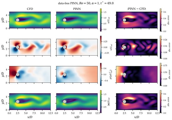
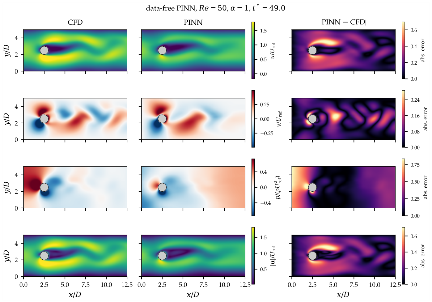
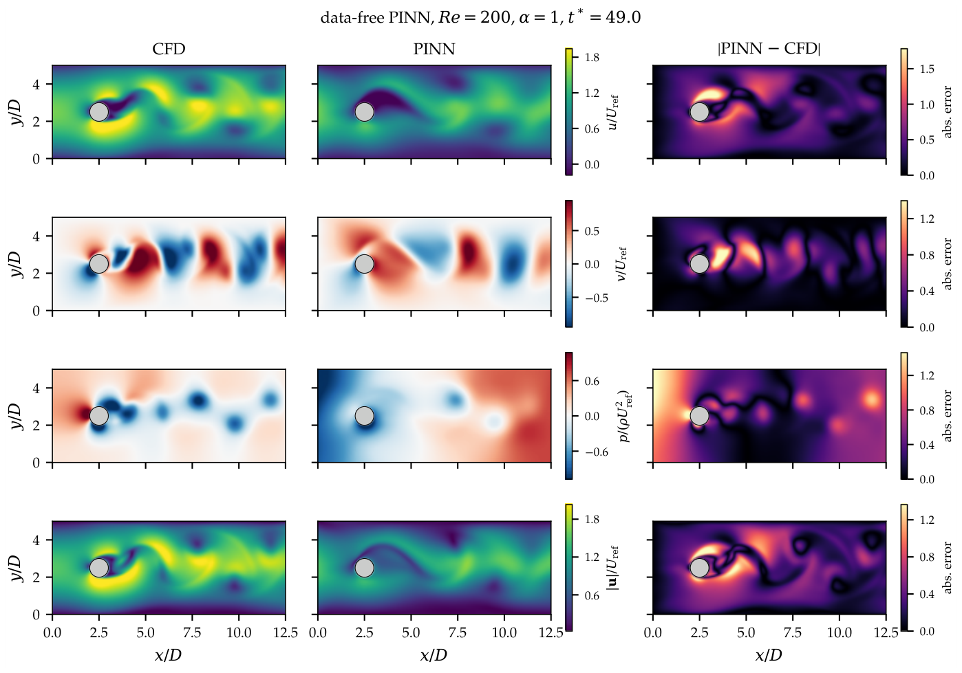
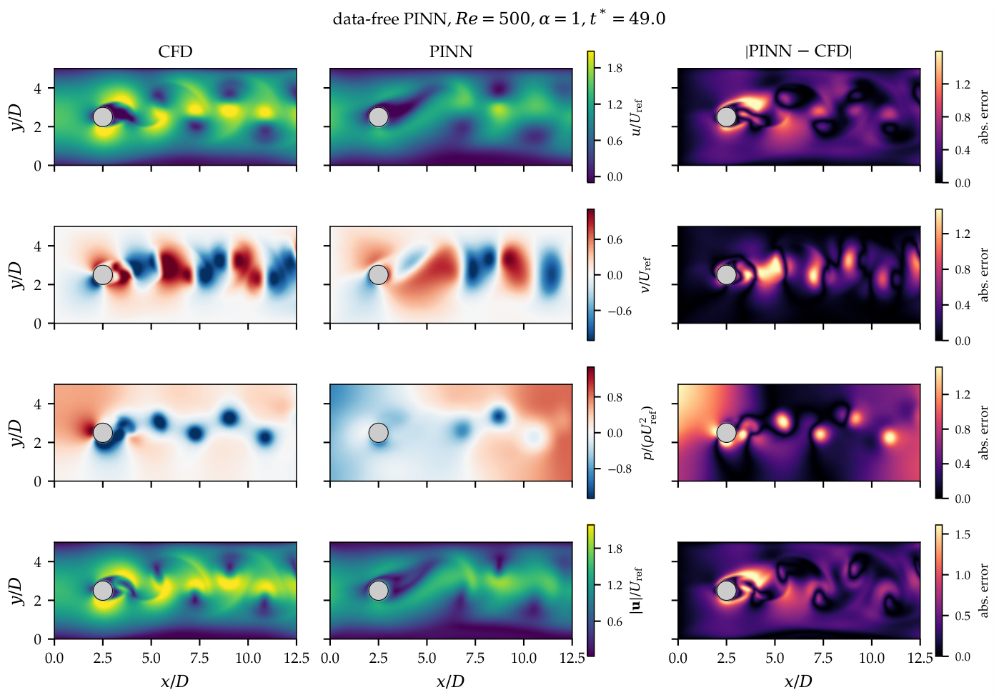
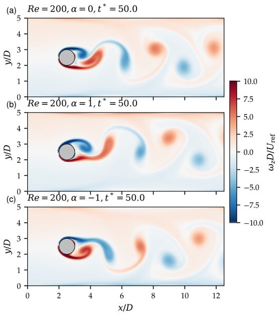
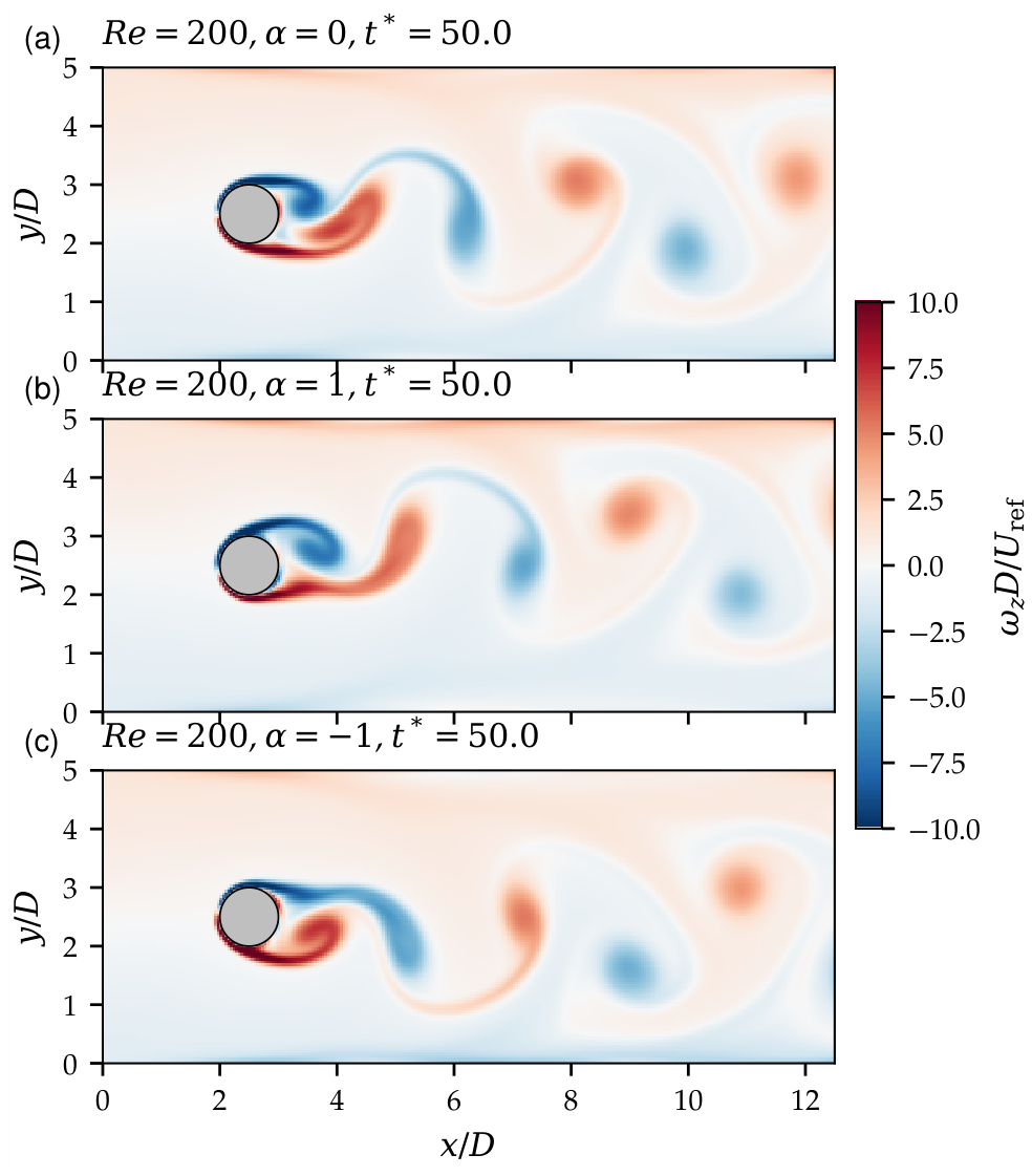
Figure 6, Figure 7 and Figure 8 compare the CFD and PINN fields for the baseline rotation ratio $\alpha =1$ at the end of the PINN interval ($t^{\ast }=49$, two time units after the CFD initial condition). Each figure shows, for u, v, p and $\left|\mathbf{u}\right|$, the CFD field, the PINN field and the absolute error on a common colour scale. Figure 9 shows the vorticity of the stationary and rotating cylinder.

Figure 6. Velocity components, pressure and velocity magnitude at $Re=50$, $\alpha =1$, $t^{\ast }=49$: CFD (left), PINN (middle) and absolute error (right).

Figure 7. As Figure 6, for $Re=200$, $\alpha =1$.

Figure 8. As Figure 6, for $Re=500$, $\alpha =1$.

Figure 9. Instantaneous vorticity at $Re=200$ (CFD) for (a) the stationary cylinder, (b) counter-clockwise rotation $\alpha =1$ and (c) clockwise rotation $\alpha =-1$, showing the deflected wake and the mirror symmetry between the two directions of rotation.

The rotation makes all fields asymmetric. The cylinder rotates counter-clockwise ($\alpha >0$), so its lower surface moves with the stream and its upper surface against it. The flow is therefore accelerated and the pressure reduced below the cylinder, whereas above it the flow is decelerated and separates earlier. The stagnation point moves downwards, the wake is deflected, and a large negative mean lift results (Magnus effect). Reversing the rotation produces the mirror image (Figure 9c). The rotation-induced flow asymmetry and wake deflection distinguish these configurations from the stationary-cylinder case.

The PINN reproduces the topology of the flow at all three Reynolds numbers: the deflected wake, the vortex street and the sign of the velocity fluctuations (Figure 6, Figure 7 and Figure 8). Quantitatively, however, the PINN fields are smoothed. Peak velocities near the cylinder are underestimated, the shed vortices are weaker and progressively out of phase, and the errors concentrate in the separating shear layers and the near wake. The pressure is the least accurate field. The PINN underestimates the pressure difference between the front and the rear of the cylinder, and its pressure level upstream of the cylinder is shifted. No pressure data enter the training, so the pressure is determined only through its gradient in the momentum equations, and it inherits the errors of the under-resolved near-wall velocity.

4.3. Error Analysis

Table 6 lists the relative $L_2$ errors of the PINN (Equation (20)), both at the end of the interval and averaged over it. Averaged over the interval, the relative error of the velocity magnitude is 14.5%, 23.4% and 24.0% at $Re=50$, 200 and 500. It grows with time from the initial condition, reaching 21%, 36% and 36% at $t^{\ast }=49$. The cross-stream velocity, whose magnitude is small, has errors of 36–51%, and the pressure errors exceed 100%. The errors are lowest at $Re=50$, where the shear layers are thicker, and similar at $Re=200$ and 500. For the stationary cylinder at $Re=200$, the errors are about half as large (9.7% for the velocity magnitude), which shows that the thin, asymmetric shear layer created by the rotating wall is a main source of error.

Table 6. Relative $L_2$ errors (%) of the PINN with respect to the CFD solution: at $t^{\ast }=49$ (${\epsilon }_q$) and averaged over $t^{\ast }\in [47,49]$ (${\overline{\epsilon }}_q$).

			${\mathit{\epsilon }}_{\mathit{q}}$ at ${\mathit{t}}^{\ast }=49$				${\overline{\mathit{\epsilon }}}_{\mathit{q}}$
Model	$\mathit{Re}$	$\mathit{\alpha }$	$\mathit{u}$	$\mathit{v}$	$\mathit{p}$	$\left|\mathbf{u}\right|$	$\mathit{u}$	$\mathit{v}$	$\mathit{p}$	$\left|\mathbf{u}\right|$
data-free	50	1	21.77	43.10	108.88	21.24	14.66	36.00	152.73	14.45
data-free	200	1	40.94	82.21	186.70	35.97	24.95	48.50	210.26	23.38
data-free	500	1	38.31	78.64	132.79	35.60	25.38	50.74	169.96	23.97
data-free	200	0	14.76	23.57	75.80	14.43	9.73	20.00	107.85	9.73
hybrid	50	1	8.76	32.65	73.44	9.28	6.86	26.19	79.44	7.26
hybrid	200	1	11.62	23.15	69.00	11.88	11.93	24.53	108.94	12.09
hybrid	500	1	12.22	24.35	65.16	12.81	11.78	22.25	80.39	11.85
hybrid + hard wall	50	1	6.26	19.54	45.92	6.55	5.86	20.06	63.91	6.08
hybrid + hard wall	200	1	9.70	21.66	68.69	10.14	11.08	20.73	102.87	11.17
hybrid + hard wall	500	1	15.54	30.68	83.95	16.41	14.57	27.34	94.27	14.60

The prediction errors in Table 6 quantify deviations from the CFD reference solution and are distinct from the residual losses evaluated during training. At the end of training, the PINN residuals are ${\mathcal{L}}_{\mathrm{PDE}}=$$1.1\times {10}^{-2}$ and ${\mathcal{L}}_{\mathrm{IC}}=$$6.2\times {10}^{-3}$ ($Re=200$). Small residuals are thus compatible with prediction errors of tens of per cent: a small residual at the collocation points does not imply a small error with respect to the true solution.

4.4. Drag and Lift Coefficients and Wake Dynamics

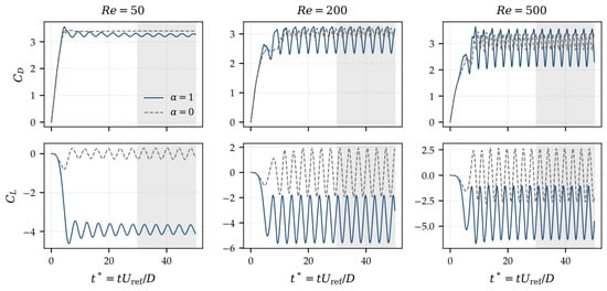
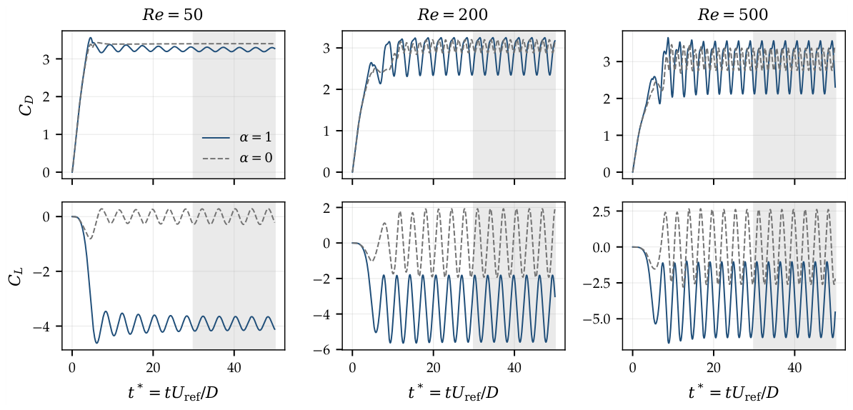
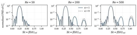
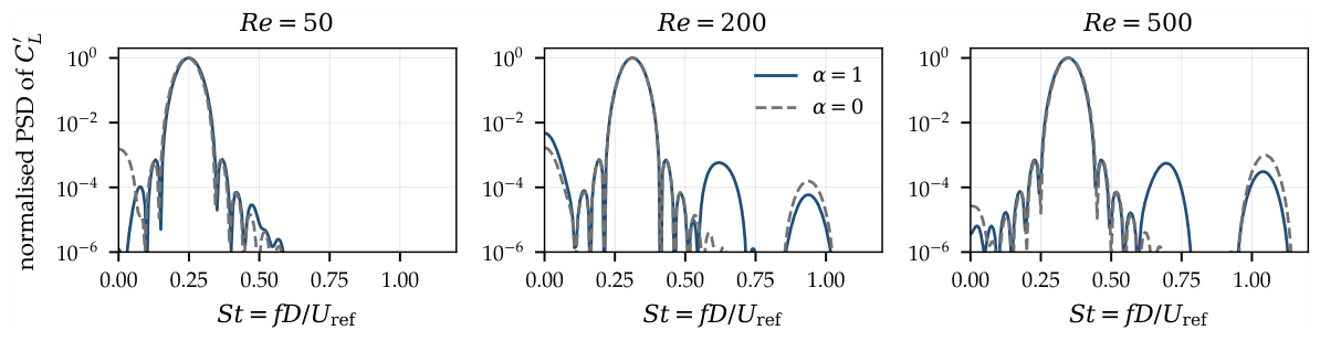
Figure 10 shows the CFD histories of $C_d$ and $C_l$ from rest to $t^{\ast }=50$ for $\alpha =0$ and $\alpha =1$, while Figure 11 shows the spectra of the lift fluctuations. The mean values, amplitudes and Strouhal numbers for the full rotation sweep are reported in Section 4.6.

Figure 10. CFD time histories of the drag (top) and lift (bottom) coefficients for $\alpha =1$ (solid) and $\alpha =0$ (dashed) at $Re=50$, 200 and 500. The grey band is the statistics window.

Figure 11. Normalised power spectral density of the lift fluctuation (CFD) for $\alpha =1$ (solid) and $\alpha =0$ (dashed). The peak defines the Strouhal number.

For a rotating cylinder, the mean lift is not zero. The circulation induced by the moving wall produces a steady Magnus force, on which the shedding-induced oscillation is superimposed. For $\alpha =1$, $\overline{C_l}=-3.91$, $-3.67$ and $-3.72$ at $Re=50$, 200 and 500, with amplitudes ${\widehat{C}}_l=0.27$, 1.89 and 2.64. The lift oscillates at the shedding frequency, $St=0.250$, 0.312 and 0.346. With rotation, the drag also oscillates at this frequency, not at twice it, because the symmetry between the two shear layers is broken. Its amplitude therefore grows from 0.16 ($\alpha =0$) to 0.45 ($\alpha =1$) at $Re=200$. The mean drag decreases with $Re$, from 3.25 to 2.89 between $Re=50$ and 200, and then stays nearly constant (2.97 at $Re=500$). The viscous contribution falls from 31% of the drag at $Re=50$ to 19% and 14% at $Re=200$ and 500. Because of the confinement ($D/H=0.2$), these values are higher than those of an unconfined cylinder.

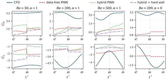
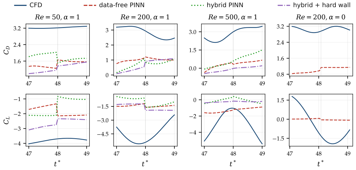
Figure 12 and Table 7 compare the forces predicted by the PINN over its interval with the CFD. The PINN predicts the sign of the Magnus lift and the order of magnitude of the forces, but it underestimates them strongly. The mean drag is underestimated by 55%, 65% and 88% and the mean lift by 52%, 68% and 54% at $Re=50$, 200 and 500. The force errors are larger than the field errors, because the forces depend on the surface pressure and the wall shear, the least accurate quantities of the PINN. A jump of the forces at the boundary between the two windows shows that the time marching does not fully enforce the continuity of the pressure. The PINN interval covers less than one shedding period, so a Strouhal number cannot be determined from the PINN forces; the shedding frequencies reported in Section 4.6 are those of the CFD.

Figure 12. Drag (top) and lift (bottom) coefficients predicted by the PINN (dashed) and the CFD (solid) over the PINN interval $t^{\ast }\in [47,49]$. The dotted line marks the boundary between the two time windows.

Table 7. Mean drag and lift coefficients and lift range over the PINN interval $t^{\ast }\in [47,49]$ (CFD and PINN). $\delta$ is the relative deviation (%) of the PINN mean.

Model	$\mathit{Re}$	$\mathit{\alpha }$	$\overline{{\mathit{C}}_{\mathit{d}}}$ CFD	PINN	$\mathit{\delta }$	$\overline{{\mathit{C}}_{\mathit{l}}}$ CFD	PINN	$\mathit{\delta }$	$\mathsf{\Delta }{\mathit{C}}_{\mathit{l}}$ CFD	PINN
data-free	50	1	3.227	1.459	54.8	−3.770	−1.824	51.6	0.373	0.811
data-free	200	1	2.851	1.011	64.5	−4.557	−1.446	68.3	3.160	0.399
data-free	500	1	2.845	0.335	88.2	−2.758	−1.281	53.5	4.390	0.748
data-free	200	0	3.058	1.017	66.7	−0.607	−0.017	97.3	3.718	0.145
hybrid	50	1	3.227	1.799	44.2	−3.770	−1.533	59.3	0.373	1.292
hybrid	200	1	2.851	0.703	75.3	−4.557	−0.994	78.2	3.160	1.206
hybrid	500	1	2.845	0.643	77.4	−2.758	−0.073	97.3	4.390	0.902
hybrid + hard wall	50	1	3.227	1.265	60.8	−3.770	−2.624	30.4	0.373	0.751
hybrid + hard wall	200	1	2.851	0.662	76.8	−4.557	−1.587	65.2	3.160	0.713
hybrid + hard wall	500	1	2.845	-0.087	103.0	−2.758	−0.249	91.0	4.390	0.224

4.5. Improved Hybrid PINN

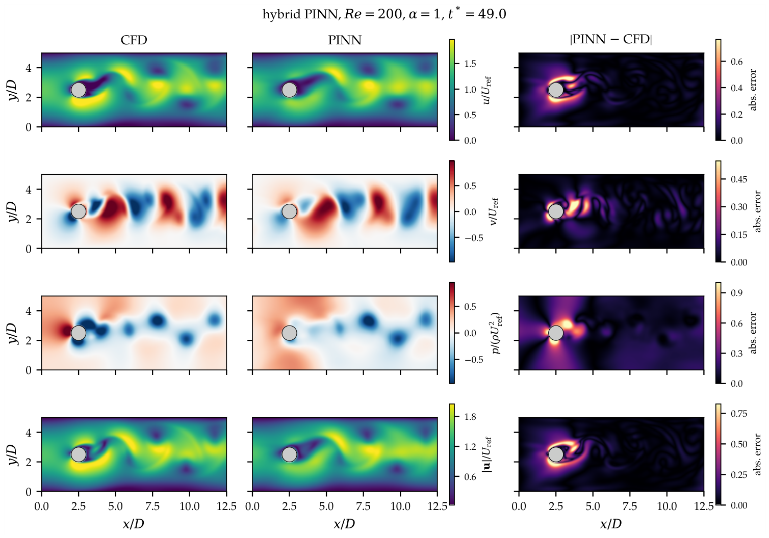
To identify which ingredients limit the accuracy, the improved hybrid PINN of Section 2.3 (near-wall sampling and sparse velocity data, about 0.4% of the cells; pressure and forces not used in training) was trained for the three $\alpha =1$ cases. Table 6 shows that the window-averaged error of the velocity magnitude is halved, from 14.5%, 23.4% and 24.0% to 7.3%, 12.1% and 11.9% at $Re=50$, 200 and 500. The pressure error, although pressure was never supplied, falls from 109–187% to 65–73% at $t^{\ast }=49$. The wake structures are visibly sharper (Figure 13). The forces, however, do not improve (Table 7): the mean drag is still underestimated by 44–77% and the mean lift by 59–97%. This ablation separates two sources of error. The bulk flow is limited mainly by the information available to the data-free network, and a small amount of velocity data corrects it effectively. The wall quantities, which control the forces, are limited by the representation of the thin rotating boundary layer itself, which sparse interior data cannot correct. Accurate force prediction with PINNs for this flow would therefore require a near-wall treatment, such as hard enforcement of the wall condition, wall-resolved sampling at the scale of the boundary layer, or a larger network, rather than more interior data. To test this explanation directly, a third variant adds a hard wall constraint to the hybrid PINN. The network output is blended with the rigid-body velocity, $\mathbf{u}=\varphi {\mathbf{u}}_{\mathcal{N}}+(1-\varphi ){\mathbf{u}}_{\mathrm{rigid}}$ with $\varphi =1-\exp [-(r-R)/0.1D]$, so the rotating-wall condition is satisfied exactly, and 35% of the collocation points are concentrated within $0.5D$ of the wall. At $Re=50$, where the boundary layer is thickest, this variant gives the best results of all: the velocity error falls to 6.1%, the pressure error to 46% at $t^{\ast }=49$, and the error in the mean lift from 59% to 30%. At $Re=200$, the field errors improve slightly (11.2%) and the lift error falls from 78% to 65%. At $Re=500$, the hard constraint does not help (14.6%), and the mean drag remains poorly predicted for all variants. The ablation thus confirms that the near-wall representation is the bottleneck. It can be relieved where the boundary layer is thick relative to the length scales that the network resolves, but not at $Re=500$ with the present network size and training budget.

Figure 13. Fields of the improved hybrid PINN at $Re=200$, $\alpha =1$, $t^{\ast }=49$: CFD (left), hybrid PINN (middle) and absolute error (right). Compare with Figure 7 (data-free PINN).

4.6. Effect of Rotation Ratio and Direction

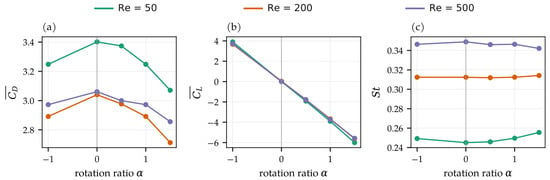
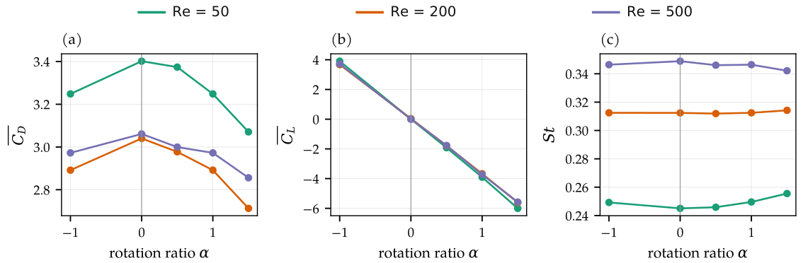
Figure 14 and Table 8 show the effect of the rotation ratio and its sign on the forces and the shedding frequency (CFD). The mean lift grows almost linearly with $\alpha$. At $Re=200$, $\overline{C_l}=-1.79$, $-3.67$ and $-5.61$ for $\alpha =0.5$, 1 and 1.5, i.e., $\overline{C_l}\approx -3.7\alpha$, and the slope is nearly independent of $Re$. At the same time the mean drag decreases, by 11% between $\alpha =0$ and $\alpha =1.5$ at $Re=200$. The rotation accelerates the boundary layer on the side where the wall moves with the stream, so it separates later there. On the opposite side, the wall moves against the stream and separation occurs earlier; the wake is deflected towards that side. Over this range of $\alpha$, the Strouhal number hardly changes (0.312–0.314 at $Re=200$), whereas the drag amplitude increases strongly (0.16 to 0.58), because the drag oscillation locks onto the shedding frequency. Clockwise rotation ($\alpha =-1$) gives the same drag, amplitude and Strouhal number as $\alpha =1$, with the mean lift reversed. This is expected, since the channel is symmetric about $y=y_c$.

Figure 14. Effect of the rotation ratio on (a) the mean drag, (b) the mean lift and (c) the Strouhal number (CFD). Negative $\alpha$ is clockwise rotation.

Table 8. Effect of cylinder rotation on the mean and amplitude of drag and lift, Strouhal number, and the pressure and viscous parts of the mean drag (CFD).

$\mathit{Re}$	$\mathit{\alpha }$	$\overline{{\mathit{C}}_{\mathit{d}}}$	${\widehat{\mathit{C}}}_{\mathit{d}}$	$\overline{{\mathit{C}}_{\mathit{l}}}$	${\widehat{\mathit{C}}}_{\mathit{l}}$	$\mathit{St}$	Pressure $\overline{{\mathit{C}}_{\mathit{d}}}$	Viscous $\overline{{\mathit{C}}_{\mathit{d}}}$
50	$-1$	3.248	0.061	3.906	0.272	0.249	2.251	0.998
	0	3.402	0.003	0.005	0.288	0.245	2.404	0.998
	$0.5$	3.374	0.034	−1.918	0.288	0.246	2.383	0.991
	1	3.248	0.061	−3.906	0.272	0.250	2.251	0.998
	$1.5$	3.071	0.056	−6.002	0.179	0.256	2.055	1.015
200	$-1$	2.892	0.453	3.673	1.887	0.312	2.342	0.550
	0	3.040	0.159	0.038	1.930	0.312	2.481	0.559
	$0.5$	2.977	0.290	−1.787	1.922	0.312	2.420	0.558
	1	2.892	0.453	−3.673	1.887	0.312	2.342	0.550
	$1.5$	2.713	0.580	−5.613	1.742	0.314	2.176	0.537
500	$-1$	2.973	0.722	3.723	2.641	0.346	2.556	0.417
	0	3.061	0.303	0.007	2.609	0.349	2.625	0.436
	$0.5$	3.000	0.468	−1.771	2.639	0.346	2.567	0.433
	1	2.973	0.722	−3.723	2.641	0.346	2.556	0.417
	$1.5$	2.856	0.941	−5.577	2.561	0.342	2.461	0.395

The present CFD results are qualitatively consistent with previous rotating-cylinder studies [28,29], demonstrating reduced mean drag and increased rotation-induced lift. When $Re=200$, the mean drag decreases by about 10.8% as the rotation ratio increases from 0 to 1.5 while vortex shedding persists. Karabelas et al. [38] reported rotation-induced wake stabilization and suppression of vortex shedding at significantly higher Reynolds numbers ($5\times {10}^5$–$5\times {10}^6$) and rotation ratios (2–8). Differences in flow regime, Reynolds number, and confinement prevent direct quantitative comparison.

4.7. Adaptive Versus Fixed Loss Weights

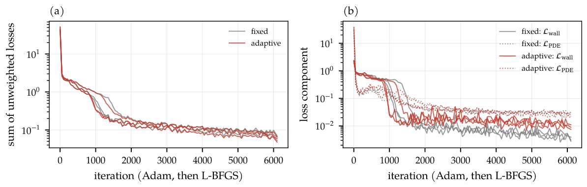
To quantify the effect of the adaptive weighting, the first time window at $Re=200$, $\alpha =1$ was trained with fixed weights (${\lambda }_k\equiv 1$) and with adaptive weights. The networks, collocation points and optimiser settings were identical, and three random seeds were used for each. Table 9 and Figure 15 give the results. With adaptive weights, the final PDE and initial-condition losses are lower than with fixed weights ($2.3\times {10}^{-2}$ versus $2.9\times {10}^{-2}$, and $1.8\times {10}^{-2}$ versus $2.7\times {10}^{-2}$), whereas the boundary and moving-wall losses are higher. The PDE loss falls below 0.05 after the same number of iterations in both cases (about 1900). The weights therefore redistribute the training effort between the loss terms rather than reducing all of them. The resulting velocity error is the same within the seed-to-seed scatter ($16.5\pm 0.8\%$ adaptive versus $16.4\pm 0.6\%$ fixed). For the present configuration, adaptive loss weighting changes the balance of the residuals but does not produce a measurable improvement in prediction accuracy compared with fixed loss weighting.

Table 9. Fixed versus adaptive loss weights ($Re=200$, $\alpha =1$, first window; mean over the seeds). The error is the window-averaged relative $L_2$ error of $\left|\mathbf{u}\right|$ (mean ± standard deviation).

Weights	Seeds	It. to ${\mathcal{L}}_{\mathbf{PDE}}<0.05$	${\mathcal{L}}_{\mathbf{PDE}}$	${\mathcal{L}}_{\mathbf{BC}}$	${\mathcal{L}}_{\mathbf{wall}}$	${\mathcal{L}}_{\mathbf{IC}}$	${\overline{\mathit{\epsilon }}}_{\left|\mathit{u}\right|}$ (%)
fixed	3	1933	2.91 $\times {10}^{-2}$	3.13 $\times {10}^{-3}$	3.25 $\times {10}^{-3}$	2.71 $\times {10}^{-2}$	16.43 ± 0.57
adaptive	3	1933	2.31 $\times {10}^{-2}$	7.33 $\times {10}^{-3}$	9.17 $\times {10}^{-3}$	1.79 $\times {10}^{-2}$	16.52 ± 0.83

Figure 15. Comparison of training convergence using fixed and adaptive loss-weighting strategies ($Re=200$, $\alpha =1$, first window, three seeds each): (a) sum of the unweighted loss terms; (b) moving-wall and PDE loss.

4.8. Computational Comparison

Table 10 separates the costs of the two methods. The hardware differs: the CFD ran on one core of a Linux server and the PINN on a desktop CPU with four threads. Neither used a GPU. The times are therefore indicative only and not a like-for-like comparison. One complete CFD run from rest to $t^{\ast }=50$, which provides the whole time history, took about 6 min. Training the PINN over its interval of two time units took about 35 min (4 CPU threads) per case. For a single configuration of this simple geometry, the PINN is therefore much more expensive than the CFD solver and also less accurate. Once trained, the PINN evaluates the full field at any $(x,y,t)$ in a fraction of a second, and its surface gradients are exact. However, the network takes only $(x,y,t)$ as inputs and is not parameterised by $Re$, $\alpha$ or the geometry, so a new configuration requires a new training, just as CFD requires a new simulation.

Table 10. Computational comparison between CFD and PINN frameworks (per case, $Re=200$, $\alpha =1$).

Parameter	CFD	PINN
Unknowns	100,000 cells × 3 variables	29,571 network parameters
Grid/collocation points	100,000 cells	37,000 points per window
Simulated interval	$t^{\ast }\in [0,50]$	$t^{\ast }\in [47,49]$ (initial state from CFD)
Iterations	20,000 time steps	2000 + 6000 Adam + 100 L-BFGS per window
Hardware	1 CPU core (Linux server)	Desktop CPU, 4 threads, no GPU
Wall time	≈6 min	about 35 min (4 CPU threads)
Field evaluation after solution	read from stored output	<1 s per snapshot
New $Re$, $\alpha$ or geometry	new simulation	new training

4.9. Discussion of Scope and Limitations

The results show where a standard data-free PINN stands for this moving-boundary problem. Started from a single CFD state, the data-free PINN follows the wake for two time units with the correct topology. Its quantitative accuracy is limited, however: velocity errors of 15–25%, larger errors in pressure, and strongly underestimated forces. Similar limitations have been reported for unsteady cylinder wakes [10,23]. We attribute them to three causes. First, fully connected tanh networks are biased towards smooth functions, and with the present network size and training budget they cannot resolve the thin shear layers created by the moving wall. Second, the pressure is determined only indirectly. Third, errors accumulate from one time window to the next. Larger networks, longer training on GPUs, adaptive sampling near the wall and causal training [13] are expected to reduce these errors, but at a cost that would further exceed that of the CFD.

Comparison with other mesh-free methods. Meshless methods based on moving least squares (MLS), such as the element-free Galerkin [39] and the meshless local Petrov–Galerkin method [40], use MLS approximants [41] on scattered nodes. They retain the convergence properties of classical discretizations. For a forward simulation in a fixed geometry, they are therefore expected to be more efficient than a PINN, consistent with [10]. A direct comparison with an MLS solver was outside the scope of this revision. The potential advantages of PINNs lie in settings that were not tested here: inverse problems, the assimilation of sparse measurements [22,27], and parametric surrogates that amortise the training over many queries.

Geometric complexity. The circular cylinder in a channel was chosen as a canonical configuration in which reliable reference data exist and the effect of rotation can be isolated. We acknowledge that it does not exploit the mesh-free character of PINNs. Geometries in which meshing is genuinely difficult are left to future work, and no advantage is claimed for them here.

5. Conclusions

This paper assessed a Physics-Informed Neural Network for the two-dimensional, time-dependent incompressible flow around a rotating circular cylinder in a channel at $Re=50$, 200 and 500, against a finite-volume solver verified on the Schäfer–Turek benchmark. The conclusions are restricted to what the results show:

• The verified CFD shows that all cases are periodic, including the stationary cylinder at $Re=50$ ($St=0.245$). For $\alpha =1$, the Magnus lift is $\overline{C_l}\approx -3.7$ to $-3.9$, and it grows almost linearly with the rotation ratio ($\overline{C_l}\approx -3.7\alpha$). The mean drag decreases by about 11% between $\alpha =0$ and 1.5, and the Strouhal number is nearly unaffected. Reversing the rotation reverses the lift and leaves drag and frequency unchanged.
• Starting from a single CFD velocity field, the data-free PINN reproduces the topology of the wake, the vortex street and the sign of the Magnus lift at all three Reynolds numbers. However, the window-averaged relative error of the velocity magnitude is 14.5%, 23.4% and 24.0% at $Re=50$, 200 and 500, and it grows with time.
• The pressure and the forces are the weakest part of the PINN prediction, because they depend on the near-wall gradients. An ablation with sparse velocity data (0.4% of the cells) halves the velocity error (to 7–12%) but does not improve the forces. Adding a hard rotating-wall constraint with boundary-layer sampling gives the best accuracy at $Re=50$ (velocity error 6.1%, lift error 30%), but its benefit vanishes at $Re=500$. The representation of the thin rotating boundary layer is therefore the limiting factor.
• The loss-magnitude-based adaptive weighting lowers the PDE and initial-condition residuals at the expense of the boundary terms, but it does not reduce the prediction error compared with fixed weights.
• For a single configuration of this simple geometry, PINN training is far more expensive than the CFD solver, and the trained network does not generalise to other $Re$, $\alpha$ or geometries.

In its present form, the PINN therefore does not constitute a superior alternative to conventional CFD for this problem. The results indicate potential in settings where mesh-free evaluation, parameterisation or data assimilation are required.

6. Future Directions

Future research will examine parametric PINNs with $Re$ and $\alpha$ as additional inputs, which could amortise the training cost over many configurations, as well as more efficient optimization methods, adaptive sampling, GPU training and hybrid PINN–CFD methodologies. Further work will address geometries in which mesh generation is genuinely difficult, three-dimensional effects at the higher Reynolds numbers, and direct comparisons with MLS-based meshless solvers. The methodology will also be explored for practical engineering problems involving rotating machinery, aerodynamic flow control, vortex-induced vibration and fluid–structure interaction.

References

- Karniadakis, G.E.; Kevrekidis, I.G.; Lu, L.; Perdikaris, P.; Wang, S.; Yang, L. Physics-informed machine learning. Nat. Rev. Phys. 2021, 3, 422–440. [Google Scholar] [CrossRef] [Scilit]
- Kim, J.; Lee, K.; Lee, D.; Jhin, S.Y.; Park, N. DPM: A novel training method for physics-informed neural networks in extrapolation. Proc. AAAI Conf. Artif. Intell. 2021, 35, 8146–8154. [Google Scholar] [CrossRef] [Scilit]
- Iskhakov, A.S.; Dinh, N.T. Physics-integrated machine learning: Embedding a neural network in the Navier–Stokes equations. Part I. arXiv 2020, arXiv:2008.10509. [Google Scholar]
- Faller, W.E.; Schreck, S.J. Unsteady fluid mechanics applications of neural networks. J. Aircr. 1997, 34, 48–55. [Google Scholar] [CrossRef] [Scilit]
- Michek, N.E.; Mehta, P.M.; Huebsch, W.W. Flight dynamics modeling using physics-informed neural networks. AIAA J. 2026, 64, 241–257. [Google Scholar] [CrossRef] [Scilit]
- Raissi, M.; Perdikaris, P.; Karniadakis, G.E. Physics-informed neural networks: A deep learning framework for solving forward and inverse problems involving nonlinear partial differential equations. J. Comput. Phys. 2019, 378, 686–707. [Google Scholar] [CrossRef] [Scilit]
- Ren, Z.; Zhou, S.; Liu, D.; Liu, Q. Physics-informed neural networks: A review of methodological evolution, theoretical foundations, and interdisciplinary frontiers toward next-generation scientific computing. Appl. Sci. 2025, 15, 8092. [Google Scholar] [CrossRef] [Scilit]
- Chen, C.; Yang, Y.; Xiang, Y.; Hao, W. Automatic differentiation is essential in training neural networks for solving differential equations. J. Sci. Comput. 2025, 104, 54. [Google Scholar] [CrossRef] [Scilit]
- Lawal, Z.K.; Yassin, H.; Lai, D.T.C.; Che Idris, A. Physics-informed neural network (PINN) evolution and beyond: A systematic literature review and bibliometric analysis. Big Data Cogn. Comput. 2022, 6, 140. [Google Scholar] [CrossRef] [Scilit]
- Grossmann, T.G.; Komorowska, U.J.; Latz, J.; Schönlieb, C.-B. Can physics-informed neural networks beat the finite element method? IMA J. Appl. Math. 2024, 89, 143–174. [Google Scholar] [CrossRef] [Scilit] [PubMed]
- Wang, S.; Sankaran, S.; Wang, H.; Perdikaris, P. An expert’s guide to training physics-informed neural networks. arXiv 2023, arXiv:2308.08468. [Google Scholar]
- Wang, S.; Teng, Y.; Perdikaris, P. Understanding and mitigating gradient flow pathologies in physics-informed neural networks. SIAM J. Sci. Comput. 2021, 43, A3055–A3081. [Google Scholar] [CrossRef] [Scilit]
- Wang, S.; Sankaran, S.; Perdikaris, P. Respecting causality for training physics-informed neural networks. Comput. Methods Appl. Mech. Eng. 2024, 421, 116813. [Google Scholar] [CrossRef] [Scilit]
- Sun, L.; Gao, H.; Pan, S.; Wang, J.X. Surrogate modeling for fluid flows based on physics-constrained deep learning without simulation data. Comput. Methods Appl. Mech. Eng. 2020, 361, 112732. [Google Scholar] [CrossRef] [Scilit]
- Meng, X.; Li, Z.; Zhang, D.; Karniadakis, G.E. PPINN: Parareal physics-informed neural network for time-dependent PDEs. Comput. Methods Appl. Mech. Eng. 2020, 370, 113250. [Google Scholar] [CrossRef] [Scilit]
- McClenny, L.D.; Braga-Neto, U.M. Self-adaptive physics-informed neural networks. J. Comput. Phys. 2023, 474, 111722. [Google Scholar] [CrossRef] [Scilit]
- Xiao, Z.; Ju, Y.; Li, Z.; Zhang, J.; Zhang, C. On the hard boundary constraint method for fluid flow prediction based on the physics-informed neural network. Appl. Sci. 2024, 14, 859. [Google Scholar] [CrossRef] [Scilit]
- Jin, X.; Cai, S.; Li, H.; Karniadakis, G.E. NSFnets (Navier–Stokes flow nets): Physics-informed neural networks for the incompressible Navier–Stokes equations. J. Comput. Phys. 2021, 426, 109951. [Google Scholar] [CrossRef] [Scilit]
- Rao, C.; Sun, H.; Liu, Y. Physics-informed deep learning for incompressible laminar flows. Theor. Appl. Mech. Lett. 2020, 10, 207–212. [Google Scholar] [CrossRef] [Scilit]
- Gao, H.; Sun, L.; Wang, J.X. PhyGeoNet: Physics-informed geometry-adaptive convolutional neural networks for solving parameterized steady-state PDEs on irregular domain. J. Comput. Phys. 2021, 428, 110079. [Google Scholar] [CrossRef] [Scilit]
- Ranade, R.; Hill, C.; Pathak, J. DiscretizationNet: A machine-learning-based solver for Navier–Stokes equations using finite volume discretization. Comput. Methods Appl. Mech. Eng. 2021, 378, 113722. [Google Scholar] [CrossRef] [Scilit]
- Raissi, M.; Yazdani, A.; Karniadakis, G.E. Hidden fluid mechanics: Learning velocity and pressure fields from flow visualizations. Science 2020, 367, 1026–1030. [Google Scholar] [CrossRef] [Scilit]
- Chuang, P.-Y.; Barba, L.A. Experience report of physics-informed neural networks in fluid simulations: Pitfalls and frustration. In Proceedings of the 21st Python in Science Conference (SciPy 2022), Austin, TX, USA, 11–17 July 2022. [Google Scholar] [CrossRef] [Scilit]
- Farea, A.; Yli-Harja, O.; Emmert-Streib, F. Understanding physics-informed neural networks: Techniques, applications, trends, and challenges. AI 2024, 5, 1534–1557. [Google Scholar] [CrossRef] [Scilit]
- Luo, K.; Zhao, J.; Wang, Y.; Li, J.; Wen, J.; Liang, J.; Soekmadji, H.; Liao, S. Physics-informed neural networks for PDE problems: A comprehensive review. Artif. Intell. Rev. 2025, 58, 323. [Google Scholar] [CrossRef] [Scilit]
- Guo, J.; Zhu, H.; Yang, Y.; Guo, C. Advances in physics-informed neural networks for solving complex partial differential equations and their engineering applications: A systematic review. Eng. Appl. Artif. Intell. 2025, 161, 112044. [Google Scholar] [CrossRef] [Scilit]
- Cai, S.; Mao, Z.; Wang, Z.; Yin, M.; Karniadakis, G.E. Physics-informed neural networks (PINNs) for fluid mechanics: A review. Acta Mech. Sin. 2021, 37, 1727–1738. [Google Scholar] [CrossRef] [Scilit]
- Kang, S.; Choi, H.; Lee, S. Laminar flow past a rotating circular cylinder. Phys. Fluids 1999, 11, 3312–3321. [Google Scholar] [CrossRef] [Scilit]
- Mittal, S.; Kumar, B. Flow past a rotating cylinder. J. Fluid Mech. 2003, 476, 303–334. [Google Scholar] [CrossRef] [Scilit]
- Stojković, D.; Breuer, M.; Durst, F. Effect of high rotation rates on the laminar flow around a circular cylinder. Phys. Fluids 2002, 14, 3160–3178. [Google Scholar] [CrossRef] [Scilit]
- Williamson, C.H.K. Vortex dynamics in the cylinder wake. Annu. Rev. Fluid Mech. 1996, 28, 477–539. [Google Scholar] [CrossRef] [Scilit]
- Fadlun, E.A.; Verzicco, R.; Orlandi, P.; Mohd-Yusof, J. Combined immersed-boundary finite-difference methods for three-dimensional complex flow simulations. J. Comput. Phys. 2000, 161, 35–60. [Google Scholar] [CrossRef] [Scilit]
- Leonard, B.P. A stable and accurate convective modelling procedure based on quadratic upstream interpolation. Comput. Methods Appl. Mech. Eng. 1979, 19, 59–98. [Google Scholar] [CrossRef] [Scilit]
- Chorin, A.J. Numerical solution of the Navier–Stokes equations. Math. Comput. 1968, 22, 745–762. [Google Scholar] [CrossRef] [Scilit]
- Liu, D.C.; Nocedal, J. On the limited memory BFGS method for large scale optimization. Math. Program. 1989, 45, 503–528. [Google Scholar] [CrossRef] [Scilit]
- Roache, P.J. Perspective: A method for uniform reporting of grid refinement studies. J. Fluids Eng. 1994, 116, 405–413. [Google Scholar] [CrossRef] [Scilit]
- Schäfer, M.; Turek, S. Benchmark computations of laminar flow around a cylinder. In Flow Simulation with High-Performance Computers II; Hirschel, E.H., Ed.; Notes on Numerical Fluid Mechanics; Vieweg: Braunschweig, Germany, 1996; Volume 48, pp. 547–566. [Google Scholar]
- Karabelas, S.J.; Koumroglou, B.C.; Argyropoulos, C.D.; Markatos, N.C. High Reynolds number turbulent flow past a rotating cylinder. Appl. Math. Model. 2012, 36, 379–398. [Google Scholar] [CrossRef] [Scilit]
- Belytschko, T.; Lu, Y.Y.; Gu, L. Element-free Galerkin methods. Int. J. Numer. Methods Eng. 1994, 37, 229–256. [Google Scholar] [CrossRef] [Scilit]
- Atluri, S.N.; Zhu, T. A new meshless local Petrov–Galerkin (MLPG) approach in computational mechanics. Comput. Mech. 1998, 22, 117–127. [Google Scholar] [CrossRef] [Scilit]
- Lancaster, P.; Salkauskas, K. Surfaces generated by moving least squares methods. Math. Comput. 1981, 37, 141–158. [Google Scholar] [CrossRef]
Disclaimer/Publisher’s Note: The statements, opinions and data contained in all publications are solely those of the individual author(s) and contributor(s) and not of MDPI and/or the editor(s). MDPI and/or the editor(s) disclaim responsibility for any injury to people or property resulting from any ideas, methods, instructions or products referred to in the content. |
© 2026 by the authors. Licensee MDPI, Basel, Switzerland. This article is an open access article distributed under the terms and conditions of the Creative Commons Attribution (CC BY) license.