


Abstract
Alpine mountain regions are shaped by interacting ecological processes. Using Aba Prefecture on the eastern Qinghai–Tibet Plateau as a case study, we derived sensitivity indices for desertification, soil erosion, landslide disaster, freeze–thaw erosion, and habitat quality for six selected study years between 2000 and 2024, and integrated them into a composite ecological sensitivity index (CESI) using the spatial distance index. We assessed class transitions, trajectories, multiscale clustering, co-sensitivity hotspots, county-level and elevation-stratified patterns, and robustness. The results showed that: (1) mean CESI rose slightly from 1.483 to 1.487, indicating marginally weaker sensitivity, but fell to 1.427 in 2020; (2) 75.86% of the area retained its initial class, with persistent low, stable moderate, and persistent high trajectories covering 48.65%, 9.29%, and 15.37%, respectively, while spatial clustering weakened at coarser scales; (3) persistent co-sensitivity hotspots covered 2900.93 km2, the dominant 2024 combination was desertification–soil erosion–freeze–thaw erosion, and over 97% of highly and extremely sensitive areas and hotspots occurred above 4000 m, indicating a pronounced concentration of ecological sensitivity and co-sensitivity hotspots in high-elevation areas; and (4) continuous sensitivity gradients were robust, whereas class assignments and high-sensitivity boundaries were more responsive to factor composition, aggregation, and scale. The findings can inform spatial planning, the prioritization of environmental monitoring and field assessment, and differentiated ecological management in alpine mountain regions.
1. Introduction
Ecological sensitivity describes how strongly an ecosystem responds to changes in the natural environment and to human disturbance. It provides an important basis for identifying potential ecological problems, delineating priority conservation areas, and guiding ecological management [1]. Under the combined effects of global climate change and human activity, alpine and high-elevation ecosystems are often especially sensitive to external disturbance because of their relatively simple structure and long recovery times [2,3]. The Qinghai–Tibet Plateau and its eastern margin are simultaneously affected by climate change, vegetation dynamics, surface erosion, and mountain hazards, and previous studies have documented pronounced spatial heterogeneity and stage-dependent changes in ecological vulnerability across this region [3,4]. Process-specific studies in Tibet have assessed freeze–thaw erosion sensitivity using climatic, topographic, and vegetation factors, providing a basis for representing cold-region processes in regional assessments [5]. Assessments based on a single ecological process therefore cannot adequately represent the coupled environmental conditions or long-term dynamics of alpine mountain regions.
Advances in remote sensing and geographic information systems (GISs) have shifted ecological sensitivity assessment from single-factor analyses toward integrated, multi-indicator frameworks. Li et al. examined the spatiotemporal evolution of terrestrial ecological sensitivity in China using biodiversity, hydrothermal conditions, desertification, soil erosion, and human disturbance [2]. Xia et al. developed an ecological vulnerability index for the Qinghai–Tibet Plateau by integrating land resources, hydroclimatic conditions, topography, and socioeconomic factors [3]. Regional assessments have also incorporated habitat sensitivity alongside soil erosion sensitivity and other environmental dimensions [6,7]. Chen et al. [8] combined habitat quality, soil erosion sensitivity, and desertification sensitivity using a spatial distance index. These studies provide a basis for incorporating habitat conservation concerns into composite ecological sensitivity assessment. For composite-index construction, Wei et al. introduced Euclidean distance into an integrated environmental sensitivity assessment and proposed a spatial distance index to reduce the compensatory effects associated with direct linear aggregation [9]. Because different erosion processes on the Qinghai–Tibet Plateau interact spatially, no single factor can fully describe composite ecological sensitivity. More recent work on the western Sichuan Plateau has incorporated desertification, soil erosion, landslides, and freeze–thaw erosion into a common assessment framework [1]. Such studies show that multi-process assessment can characterize the integrated sensitivity of alpine environments more comprehensively than a single-factor approach. Nevertheless, a composite index primarily expresses overall sensitivity and does not directly reveal where individual processes co-occur or persist over time.
Despite these advances, three issues warrant further attention. First, most studies emphasize the spatial distribution of index values and sensitivity classes, with less attention to the persistence and transition of sensitivity states over long time series. Combining transition matrix analysis with multi-period trajectory classification provides a methodological basis for distinguishing persistent sensitivity states from temporal transitions and fluctuations [10,11]. Second, although a composite index represents overall regional sensitivity, it can obscure the specific spatial combinations of high values among individual indices, making it difficult to identify which sensitivity components are simultaneously high in the same area. Studies of ecosystem services have shown that applying a common quantile threshold and overlaying the resulting high-value areas can effectively reveal multi-process hotspots and their combinations [12,13,14,15], providing a useful basis for co-sensitivity analysis. Hotspot persistence across multiple years can further inform the identification of potential long-term conservation priorities [16]. Third, ecological sensitivity results depend on analytical choices such as spatial scale, indicator composition, normalization, and aggregation [17,18,19,20]. The stability of composite ecological sensitivity patterns can be evaluated by systematically varying assessment settings and model specifications, following the principles of sensitivity analysis [21].
Aba Prefecture lies on the southeastern margin of the Qinghai–Tibet Plateau. Its pronounced topographic relief, interspersed alpine grasslands, forests, wetlands, and alpine bare land, and concurrent exposure to desertification, soil erosion, freeze–thaw processes, and mountain hazards make it a representative setting for studying composite ecological sensitivity in an alpine mountain region. We therefore used multi-source data for six years between 2000 and 2024 to construct a five-dimensional assessment system covering desertification, soil erosion, landslide disaster, freeze–thaw erosion, and habitat quality. By combining multi-process assessment with multi-period trajectories, co-sensitivity hotspots, multiscale spatial analysis, and robustness tests, this study aims to identify long-term ecological sensitivity cores and their dominant process combinations across Aba Prefecture and to provide evidence for alpine ecosystem conservation and spatially differentiated management. Previous studies have assessed composite ecological sensitivity at different regional scales and examined its spatiotemporal variation and associated factors [1,2,3,22]. Building on this work, the main contribution of the present study is the integrated application of established assessment and analytical methods. The resulting framework combines multi-period sensitivity-class trajectories, the spatial combinations and persistence of co-sensitivity hotspots, and model robustness tests to systematically characterize the spatiotemporal evolution and spatial differentiation of composite ecological sensitivity in Aba Prefecture and provide a spatial basis for ecological conservation and management in alpine mountain regions.
2. Materials and Methods
2.1. Study Area
Aba Tibetan and Qiang Autonomous Prefecture is located in northwestern Sichuan Province on the southeastern margin of the Qinghai–Tibet Plateau, between approximately 100°30′–104°27′ E and 30°35′–34°19′ N. It comprises 13 counties and county-level cities (Figure 1). The terrain is highly dissected, with a mean elevation above 3000 m, and supports a mosaic of forests, alpine grasslands, wetlands, and alpine bare land. The combination of complex natural conditions and human disturbance makes these ecosystems susceptible to disruption and slow to recover, providing a representative setting for composite ecological sensitivity assessment.
Figure 1.
Location of the study area.
2.2. Data Sources and Preprocessing
The data used in this study included geological and geomorphological, meteorological, vegetation, and land-cover data spanning 2000–2024 (Table 1). All datasets were subjected to projection, clipping, registration, and other necessary preprocessing. The geographic coordinate system was standardized to the World Geodetic System 1984 (WGS 1984) and the projected coordinate system to Albers. The spatial resolution was standardized to 1000 m × 1000 m.
To limit information loss during spatial harmonization, a common 30 m computational grid was first established in an Albers equal-area projection. During reprojection or grid alignment, bilinear interpolation was applied to the digital elevation model (DEM) and nearest-neighbor resampling to China Land Cover Dataset (CLCD) data; terrain and land-cover factors were then derived from these aligned layers. Road and river vectors were used to generate 30 m Euclidean distance rasters, and the 90 m soil erodibility factor (K) was aligned using bilinear interpolation. Fractional vegetation cover, annual precipitation, annual temperature range, and rainfall erosivity were calculated from the normalized difference vegetation index (NDVI) and meteorological data at their native 1 km resolution. When used in the 30 m assessments, these variables were matched to the computational grid by nearest-neighbor resampling. This conversion was used for spatial alignment and did not add spatial information to the original coarse-resolution data. The finer-resolution terrain, land-cover, and distance factors could represent corresponding local differences, whereas the vegetation and meteorological variables remained constrained by their original 1 km resolution and could not independently resolve sub-kilometer variation. Thus, using a 30 m computational grid does not imply that all information contributing to each index has 30 m spatial detail.
The land desertification sensitivity index (LDSI) was calculated at 1 km resolution, whereas the soil erosion sensitivity index (SESI), landslide disaster sensitivity index (LSI), and freeze–thaw erosion sensitivity index (FESI) were constructed at 30 m resolution, and the habitat sensitivity index (HSI) was obtained from the 30 m output of the Integrated Valuation of Ecosystem Services and Tradeoffs (InVEST) Habitat Quality model. The four 30 m indices were aggregated to 1 km using valid-area-weighted means. For partially covered grid cells, weights were based on the areas of valid constituent 30 m pixels. A common valid-data mask was applied across all six study years, yielding an analysis area of 82,474.83 km2. The six-period 1 km observations for each component were then pooled to determine common normalization bounds, after which the composite ecological sensitivity index (CESI) was calculated. Finally, the 1 km CESI was aggregated by area-weighted averaging to 5 and 10 km to assess the effects of spatial aggregation. Accordingly, CESI and co-sensitivity hotspots were interpreted at the final 1 km assessment scale, with emphasis on relative regional patterns and their changes over time. The delineated local boundaries remained affected by input resolution and spatial aggregation; finer-scale applications require support from higher-resolution data.
Due to the limited availability of temporally consistent and sufficiently complete historical road network data, we followed previous multi-temporal landslide studies that treated road proximity as a fixed spatial factor [23]. Accordingly, the OpenStreetMap road network extracted on 1 January 2024 was used as a common spatial reference for all six study years. However, this network does not fully represent the actual road conditions in earlier years.
Table 1.
Data sources and characteristics.
2.3. Methods
Using multi-source remote sensing, geographic, and meteorological data for 2000–2024, we constructed sensitivity indices for desertification, soil erosion, landslide disaster, freeze–thaw erosion, and habitat quality. After normalizing the indices to a common numerical range while retaining their component-specific ecological meanings, the five indices were integrated into the CESI using the spatial distance index. We then examined spatiotemporal change, spatial clustering, co-sensitivity hotspots, and county-level and elevation-level differences, followed by robustness and uncertainty analyses (Figure 2).
Figure 2.
Research workflow. Abbreviations: CESI, composite ecological sensitivity index; VFC, fractional vegetation cover; DEM, digital elevation model; RUSLE, Revised Universal Soil Loss Equation; AHP, analytic hierarchy process; InVEST, Integrated Valuation of Ecosystem Services and Tradeoffs; LISA, local indicators of spatial association; FESI, freeze–thaw erosion sensitivity index; HSI, habitat sensitivity index; RMSE, root mean square error; P80, 80th percentile; SD, standard deviation; P1–P99, 1st–99th percentile normalization; H/S, habitat suitability and threat sensitivity.
2.3.1. Composite Ecological Sensitivity Index
- Land Desertification Sensitivity Index
Desertification sensitivity represents the potential for land degradation and sandification under climatic aridity, wind action, vegetation degradation, and human disturbance [26]. Northwestern Aba Prefecture is characterized by high elevations, cold and dry conditions in some areas, and slow vegetation recovery. Once vegetation cover declines, exposed surfaces become more susceptible to wind erosion and other disturbances. We represented desertification conditions using fractional vegetation cover, estimated from the normalized difference vegetation index (NDVI) [27], and used it to calculate the land desertification sensitivity index.
where VFC is fractional vegetation cover; NDVI is the pixel-level normalized difference vegetation index; and NDVImax and NDVImin are the maximum and minimum NDVI values, respectively. The land desertification sensitivity index was calculated as LDSI = 1 − VFC. Higher LDSI values indicate lower vegetation cover and greater relative sensitivity to desertification. To ensure comparability of fractional vegetation cover estimates across study years, common NDVI maxima and minima were determined from the pooled data for all six study years.
- 2.
- Soil Erosion Sensitivity Index
Assessment factors were selected within the process framework of the Revised Universal Soil Loss Equation (RUSLE) [28]. Rainfall erosivity (R) was calculated from monthly and annual precipitation using the empirical equations proposed by Renard and Freimund [29]. Soil erodibility (K) was estimated from sand, silt, clay, and organic carbon contents [30]. The slope length and steepness factor (LS) was derived from a 30 m digital elevation model (DEM). The cover-management factor (C) was calculated from fractional vegetation cover using the relationship proposed by Cai et al. [31]. The support-practice factor (P) was assigned by CLCD land-cover class using the coefficients reported by Chen et al. [1], as listed in Table S1.
where f represents vegetation cover expressed as a percentage (0–100), and C denotes the cover-management factor.
where SESI is the soil erosion sensitivity index; R is rainfall erosivity; K is soil erodibility; LS is the slope length and steepness factor; C is the cover-management factor; and P is the support-practice factor.
SESI = R × K × LS × C × P
- 3.
- Landslide Disaster Sensitivity Index
The landslide disaster sensitivity index represents the relative tendency of a spatial unit to experience slope instability under a given combination of topographic, hydroclimatic, land-cover, and anthropogenic conditions [32]. Based on factor selection in previous landslide susceptibility studies and the characteristics of Aba Prefecture, six factors were used: slope, elevation, distance to roads, distance to rivers, land use, and annual precipitation [33,34]. The factor weights were adopted from the work of Zheng et al. [34], who applied the Analytic Hierarchy Process (AHP) to landslide hazard assessment in Maoxian County, Aba Prefecture. Their AHP framework comprised three levels: the overall objective, criteria, and indicators. The criterion level included anthropogenic engineering activities (roads), natural environmental conditions (slope, elevation, rivers, and land use), and triggering factors (precipitation). Pairwise comparison matrices were constructed for the criterion level and the natural-environment subgroup. At the criterion level, the comparison values for anthropogenic activities versus natural conditions, anthropogenic activities versus triggering factors, and natural conditions versus triggering factors were 1, 2, and 4, respectively. Within the natural-environment subgroup, elevation and distance to rivers were assigned comparison values of 4 and 5 relative to slope, respectively. The original study reported consistency ratios (CR) of 0.0516 and 0.0952 for the two matrices, respectively, both below the acceptable threshold of 0.1. The complete pairwise comparison matrices and their corresponding weights are presented in Table S2. The resulting weights for the six selected factors were 0.0559, 0.2203, 0.3764, 0.1496, 0.0484, and 0.1494, respectively.
The classification thresholds and scores were specified for this study with reference to regional landslide susceptibility studies [35,36,37,38]. The detailed classification and scoring rules are provided in Table S3.
- 4.
- Freeze–Thaw Erosion Sensitivity Index
Freeze–thaw erosion occurs when repeated freezing and thawing loosens soil structure and fragments particles, which are subsequently transported by snowmelt runoff, surface runoff, and gravity [5]. High-elevation areas of Aba Prefecture experience low temperatures and pronounced diurnal and seasonal temperature ranges, making freeze–thaw processes widespread. Following the work of Wang et al. [39], five factors were selected to assess freeze–thaw erosion sensitivity: annual temperature range, annual precipitation, slope, aspect, and fractional vegetation cover. Their weights were adopted directly from the expert judgment and analytic hierarchy process (AHP) scheme reported in that study and were 0.1, 0.2, 0.4, 0.1, and 0.2, respectively. The same five-factor weighting scheme was also used by Zhao et al. [22] in a composite ecological sensitivity assessment of the Qinghai–Tibet Plateau. Wang et al. [39] did not report the corresponding judgment matrix or consistency ratio (CR); the consistency of the original AHP judgments therefore could not be independently verified from the published information. To assess the influence of the adopted weights on the composite assessment, we used the five-factor weights reported by Chen et al. [1] for the western Sichuan Plateau as an alternative scheme, recalculated FESI and CESI, and evaluated agreement with the baseline results. The methods and results are presented in Section 2.3.6 and Section 3.6. The potential freeze–thaw erosion zone was delineated using the latitude- and longitude-dependent lower elevation limit described by Wang et al. [39]. Within this zone, the five factors were assigned sensitivity scores of 1–4, and FESI was calculated as their weighted sum. Following the distinction between sensitive and insensitive areas used by Li et al. [40], areas outside the delineated zone were classified as insensitive and assigned an FESI value of 0, distinguishing them from the lowest sensitivity score within the zone. The factor classification and scoring rules are provided in Table S4.
- 5.
- Habitat Sensitivity Index
Previous regional studies have incorporated habitat sensitivity alongside sensitivities to adverse ecological processes in composite assessments [8,41,42]. Chen et al. [8] combined habitat, soil erosion, and land desertification sensitivity; Chen et al. [41] integrated habitat, soil erosion, desertification, and salinization sensitivity; and Liu et al. [42] jointly assessed land desertification, soil erosion, soil salinization, and habitat sensitivity. These studies represented the habitat dimension using information such as species richness, land-cover type, vegetation cover, and habitat quality, assigning higher habitat sensitivity scores to areas with better natural habitat conditions, greater species richness, or higher habitat quality [8,41,42].
Following this multidimensional approach, which assesses habitat alongside adverse ecological processes, we included habitat sensitivity together with desertification, soil erosion, landslide, and freeze–thaw erosion sensitivity in CESI to account for the erosion and geological-hazard characteristics of Aba Prefecture’s alpine environment. Because comprehensive data on species distributions and abundance were difficult to obtain, we followed Chen et al. [8] and directly used the InVEST habitat quality index as a proxy for habitat sensitivity, with HSI = Q and no inverse transformation.
Q integrates habitat suitability, external threats, and the sensitivity of different habitat types to those threats. It ranges from 0 to 1, with higher values indicating better-modeled habitat conditions [43]. Within the composite assessment framework adopted here, higher Q values were assigned higher habitat sensitivity scores to reflect conservation attention to high-quality habitats. This scoring convention does not imply that high-quality habitats are necessarily more susceptible to damage under the same external disturbance.
where Dxj is the habitat degradation degree of habitat type j; R is the number of threat sources; wr is the weight of threat r; Yr denotes the threat-source grid; Ry is the stress value at grid cell y; Rrxy represents the influence of threat x on grid cell y within habitat x; βx denotes accessibility; Sjr is the sensitivity of habitat type j to threat r; Qxj represents relative habitat quality; k is the half-saturation constant; Hj is habitat suitability; and z is the scaling constant.
Habitat quality was assessed using the Habitat Quality module of InVEST version 3.14.2. Following the InVEST model documentation and previous studies [43], the half-saturation constant (k) was set to 0.05, and the scaling constant (z) was fixed at 2.5. As no spatial accessibility constraints were specified, the threat accessibility coefficient (βₓ) was uniformly set to 1 across the study area, without introducing additional restrictions on threat accessibility. Consistent model parameters were applied across all six study periods to ensure temporal comparability of the habitat quality assessments. Following previous studies [44,45], cropland, built-up land, and bare land were selected as habitat threat sources. Their maximum influence distances, weights, and decay functions were adopted from Yang et al. [46]. The threat source parameters and the habitat suitability and threat sensitivity values for different land-cover types are provided in Tables S5 and S6, respectively.
- 6.
- Composite Ecological Sensitivity
No single-factor index can fully represent the interacting ecological concerns faced in regional management. We therefore integrated the five sensitivity indices using the spatial distance index [9]. To clarify the ecological meanings and value directions of the different indicators, Table 2 summarizes the interpretation of high and low values for the five single-factor sensitivity indices. The five indices were normalized using the min–max method. For each index, the minimum and maximum values were determined from valid grid cells pooled across all six study years and applied consistently to each year (Table S7). The normalization was calculated as follows:
where Xi and Si represent the original and normalized values of the ith sensitivity index, respectively, and Xi,min and Xi,max are its minimum and maximum values pooled across the six study years.
Table 2.
Ecological interpretation of high and low values of the five sensitivity indices.
The five indices follow a common scoring direction in the composite assessment while retaining their distinct ecological meanings. Higher values of the four process-related indices indicate greater potential sensitivity to the corresponding ecological processes, whereas higher HSI values indicate higher conservation-oriented habitat sensitivity scores. Min–max normalization places the indices on a common numerical range without removing these differences in ecological meaning.
The normalized indices form a five-dimensional assessment space, in which the fixed reference point (1, 1, 1, 1, 1) represents a theoretical combination of the highest assessment scores in all five dimensions. CESI is the Euclidean distance between each grid cell and this reference point; a smaller distance indicates higher relative composite ecological sensitivity under the adopted assessment framework. The result integrates five dimensions rather than representing the sensitivity of a single ecological process, and a high composite sensitivity class does not require high values in every component.
where Si is the ith normalized single-factor sensitivity index (i = 1, 2, …, 5), corresponding to LDSI, SESI, LSI, FESI, and HSI, and Si,max is its maximum value. LDSI denotes the land desertification sensitivity index, SESI the soil erosion sensitivity index, LSI the landslide disaster sensitivity index, FESI the freeze–thaw erosion sensitivity index, and HSI the habitat sensitivity index; the subscript max denotes the maximum of the corresponding index. A numerical example of CESI calculation is provided in Supplementary Methods S1.
The baseline normalization retained valid extreme values without percentile-based trimming; P1–P99 winsorized normalization was used only in a separate robustness analysis to assess the influence of extreme values on the results. During normalization and CESI integration, a common valid-data mask was applied across all five sensitivity indices and six study years, excluding any grid cell containing NoData or non-finite values in any component or year.
To ensure comparability through time, valid CESI observations from all six years were pooled into a single distribution containing all valid grid-cell values, and a common set of thresholds defining five sensitivity classes was determined using the Jenks natural breaks method [47]. The same thresholds were then applied to every year. Classes 1–5 represent insensitive, slightly sensitive, moderately sensitive, highly sensitive, and extremely sensitive conditions, respectively. Because lower CESI values indicate greater sensitivity, CESI values from high to low correspond to sensitivity classes 1–5 from low to high. The corresponding CESI ranges for the five sensitivity classes are presented in Table 3.
Table 3.
Classification criteria for the composite ecological sensitivity index (CESI).
2.3.2. Spatiotemporal Change, Class Transitions, and Trajectories
For each study year, we calculated the mean and standard deviation of CESI and the area share of each sensitivity class. Area-based transition matrices were then used to quantify changes between sensitivity classes [10]. A 5 × 5 matrix was constructed for each consecutive interval (2000–2005, 2005–2010, 2010–2015, 2015–2020, and 2020–2024) and for the full period (2000–2024):
where Sij is the area that changed from sensitivity class i at the beginning of the period to class j at the end, i and j denote the initial and final classes, respectively, and n = 5. Diagonal elements represent class persistence, whereas off-diagonal elements represent transitions between classes.
Following grid-based coding approaches for multi-period ecological sensitivity [2,11], the six CESI class maps were encoded and classified into long-term trajectories using the full sequence and the difference between the first and last years. Grid cells in classes 1–2 throughout all six years were defined as persistent low sensitivity; cells in class 3 throughout were defined as stable moderate sensitivity; and cells in classes 4–5 throughout were defined as persistent high sensitivity. Among the remaining cells, those with the same initial and final class but one or more intermediate changes were classified as fluctuating unchanged. Cells whose final class was higher than their initial class were classified as fluctuating increase, and those whose final class was lower were classified as fluctuating decrease. This procedure produced six long-term trajectory types: persistent low, stable moderate, persistent high, fluctuating unchanged, fluctuating increase, and fluctuating decrease.
2.3.3. Multiscale Spatial Autocorrelation and Local Clustering
The 1 km CESI grids were aggregated to regular grids of 1, 5, and 10 km. Each target cell was assigned the area-weighted mean of its valid constituent cells. Because spatial aggregation can alter statistical relationships and mapped patterns, comparisons across these scales were used to evaluate sensitivity to spatial support [48].
- Global Moran’s I
Global Moran’s I was used to quantify overall spatial autocorrelation in CESI [49]:
where I is Global Moran’s I; n is the number of grid cells; xi and xj are the CESI values for grid cells i and j, respectively; is the mean CESI; wij is the spatial weight between grid cells i and j; and S0 is the sum of all spatial weights.
A binary spatial-weight matrix was constructed using first-order Queen contiguity: wᵢⱼ = 1 when two valid grid cells shared an edge or vertex and 0 otherwise, with wᵢᵢ = 0. Separate spatial-weight matrices were constructed at 1, 5, and 10 km, and Global Moran’s I was calculated at each scale. Two-sided pseudo-p values were obtained from 9999 random permutations to assess spatial clustering in composite ecological sensitivity and its variation across scales.
- 2.
- Local Moran’s I
Local indicators of spatial association (LISA) were calculated at 5 km to balance local spatial detail, pattern continuity, and computational demand [50]. Because lower CESI values indicate greater sensitivity, CESI was directionally transformed before LISA analysis so that higher transformed values represented greater sensitivity. Accordingly, high–high (HH) and low–low (LL) clusters denote clusters of high and low ecological sensitivity, respectively. Local Moran’s I for grid cell i was calculated as follows:
where Ii is Local Moran’s I for grid cell i; m2 is the second central moment of CESI; xi and xj are the CESI values for grid cells i and j; is the mean CESI; and wij is the spatial weight between grid cells i and j. Local Moran’s I also used first-order Queen contiguity at 5 km. The binary contiguity weights were row-standardized by dividing each neighbor’s weight by the number of valid neighbors of the focal grid cell, so that the weights summed to 1 for each non-isolated cell. Local significance was assessed using 999 conditional random permutations, and the Benjamini–Hochberg procedure was applied to control the false discovery rate across multiple tests, with a significance threshold of q ≤ 0.05 [51,52].
2.3.4. Multi-Factor Co-Sensitivity Hotspots
- Threshold-Based Co-Sensitivity Analysis
To identify the spatial overlap of high values among the five modeled sensitivity indices, their high-value areas were overlaid using threshold-based approaches from studies of ecosystem multifunctionality and ecosystem service hotspots [12,13]. The number of indicators simultaneously meeting a specified threshold within the same spatial unit was used to represent the degree of multi-factor co-occurrence [13]:
where MFt is the number of indicators meeting threshold t; F is the total number of indicators; fi is the ith indicator; ri(·) denotes the directional transformation of that indicator; and ti is the corresponding threshold. The indicator function equals 1 when the condition is met and 0 otherwise.
Previous studies commonly use the upper 20% of an indicator distribution to identify high-value areas [14,15] and define multi-service hotspots where a majority of indicators co-occur [14]. Here, valid normalized observations for each sensitivity index were pooled across all six years, and the 80th percentile (P80) was calculated as a fixed, cross-period threshold. Pooling observations across the six study years established a common cross-period high-value criterion for each index, allowing changes in hotspots to be compared against the same threshold. A grid cell was identified as a multi-factor co-sensitivity hotspot when at least three of the five indices met or exceeded their respective P80 thresholds. UpSet analysis was used to quantify the intersections and areas of different sets of highly sensitive factors and to identify the dominant co-sensitivity combinations [53]. Spearman’s rank correlations among the five single-factor indices were also calculated from the pooled six-period sample to aid interpretation of these combinations.
We then counted the number of years in which each grid cell was identified as a co-sensitivity hotspot (0–6) to characterize temporal persistence. Cells classified as hotspots in all six years were defined as persistent co-sensitivity hotspots [16].
To examine how shared inputs affected statistical associations among components, we identified the environmental variables and derived representations used by multiple indices and applied spatially blocked holdout prediction. Associations between continuous component indices and between their P80 high-value indicators were compared before and after controlling for the relevant inputs. The diagnostic methods and shared inputs are described in Supplementary Methods S2 and Table S8, and the diagnostic results are presented in Table S9.
- 2.
- Threshold Sensitivity Test
Co-sensitivity hotspots were recalculated using four alternative definitions of high sensitivity: fixed single-factor Jenks classes 4 or 5, pooled six-period P75 and P85 thresholds, and P80 thresholds calculated separately for each year. These results were compared with the pooled six-period P80 baseline. Let A denote the hotspot set identified using the pooled P80 baseline and B the set identified using the corresponding alternative criterion. Their spatial overlap was evaluated using the Jaccard index [54]:
where |A ∩ B| and |A ∪ B| are the intersection and union areas of the two hotspot sets, respectively. Values closer to 1 indicate greater spatial agreement. Annual hotspot area and the area of persistent hotspot cores across all six study years were also compared among scenarios to assess the sensitivity of hotspot extent and persistence to the high-value criterion.
2.3.5. County-Level and Elevation-Stratified Statistics
To improve the management relevance of the results, county-level and elevation-stratified statistics were calculated within the common valid-data mask. For each of the 13 counties and county-level cities, we summarized the annual area-weighted mean CESI, the area classified as highly or extremely sensitive, the co-sensitivity hotspot area, and the change from 2000 to 2024.
The DEM was used to divide the study area into six elevation bands: <2500, 2500–3000, 3000–3500, 3500–4000, 4000–4500, and ≥4500 m. Valid area, mean CESI, highly and extremely sensitive area, and co-sensitivity hotspot area were calculated for each band.
2.3.6. Uncertainty and Robustness
- Weight Uncertainty
Monte Carlo simulation was used to assess uncertainty in the indicator weights [18,19]. To ensure non-negative weights summing to 1, random weights were generated from a Dirichlet distribution centered on the baseline of equal weights for the five components:
where w0 is the baseline weight vector (0.2, 0.2, 0.2, 0.2, 0.2), and κ is the Dirichlet concentration parameter controlling the dispersion of random weights around the baseline. Following the parameter setting in an existing spatial assessment using five equally weighted indicators [55], κ = 100 was selected as the baseline perturbation scenario. The theoretical standard deviation of each weight was approximately 0.040, equivalent to 20% of the baseline weight. To examine sensitivity to perturbation magnitude, two additional scenarios were specified with κ = 25 and 400, corresponding to theoretical standard deviations of approximately 0.078 and 0.020, respectively. Each scenario comprised 1000 random simulations. For each Monte Carlo realization r, the sampled weights were incorporated into the spatial-distance formulation as follows:
where is the sampled weight of component i in realization r. The factor of 5 preserves the scale of the original CESI; when for all five components, the weighted formulation reduces exactly to Equation (7).
Spearman’s rank correlation coefficient, the baseline class retention rate, and the Jaccard index for highly and extremely sensitive areas were used to evaluate the stability of continuous CESI spatial rankings, sensitivity-class assignments, and the spatial overlap of highly sensitive areas, respectively.
- 2.
- Model Robustness
Internal robustness was tested in four ways: removing each sensitivity factor in turn and recalculating CESI; replacing spatial-distance aggregation with an equal-weight arithmetic mean; replacing the original normalization with P1–P99 winsorized min–max normalization; and comparing the 5 and 10 km aggregation results with the 1 km baseline.
Following the leave-one-factor-out tests, the two components whose omission most affected agreement with the baseline in CESI sensitivity classes and highly and extremely sensitive areas were selected for internal-parameter robustness tests. For freeze–thaw erosion sensitivity, the five-factor weights reported by Chen et al. [1] for the western Sichuan Plateau were used as an alternative. The weight for annual temperature range increased from 0.100 to 0.543, whereas that for slope decreased from 0.400 to 0.263, shifting the dominant weighting from slope to annual temperature range. The weights for annual precipitation, aspect, and fractional vegetation cover changed from 0.200, 0.100, and 0.200 to 0.117, 0.049, and 0.028, respectively. For habitat sensitivity, habitat suitability (H) and sensitivity to threats (S), which enter the InVEST habitat quality calculation directly, were selected for joint perturbation. Following the joint-perturbation approach and ±20% magnitude used by Wu et al. [56], two scenarios were specified: Higher-Q (H increased by 20% and S decreased by 20%) and Lower-Q (H decreased by 20% and S increased by 20%). Because both H and S range from 0 to 1, perturbed values were clipped to this range, and parameters originally equal to zero remained zero. All other parameters were held fixed. The corresponding component indices and CESI were recalculated to assess how the selected internal-parameter changes affected the composite assessment.
For each alternative specification, the overlap of highly and extremely sensitive areas with the baseline was measured using the Jaccard index [54], agreement in the spatial ranking of continuous CESI was assessed using Spearman’s rank correlation coefficient [57], and agreement among the five sensitivity classes was assessed using quadratic-weighted Cohen’s kappa [58]. In addition, root mean square error (RMSE) was used to quantify numerical differences in CESI between the internal-parameter scenarios and the baseline.
3. Results
3.1. Spatiotemporal Changes in Composite Ecological Sensitivity
Mean CESI values for the six study years were 1.483, 1.463, 1.455, 1.496, 1.427, and 1.487, respectively. Because a lower CESI indicates greater sensitivity, composite ecological sensitivity intensified progressively from 2000 to 2010, weakened in 2015, reached its highest level among the six years in 2020, and returned in 2024 to a level close to that observed in 2000 (Figure 3; Table 4). From 2000 to 2024, prefecture-wide mean CESI increased by only 0.004, substantially less than the changes between consecutive study years. Composite ecological sensitivity was therefore broadly similar at the beginning and end of the study period, despite marked fluctuations during the intervening years.
Figure 3.
Composite ecological sensitivity classes for the six study years.
Table 4.
Ecological sensitivity statistics by year.
Changes in the combined area share of the highly and extremely sensitive classes were consistent with changes in the continuous mean. These two classes accounted for 17.53%, 18.91%, 18.28%, 16.32%, 19.65%, and 17.15% of the study area in the six respective years. Their combined share was greatest in 2020, when soil erosion, landslide disaster, and freeze–thaw erosion sensitivities were also relatively high. This concurrence indicates that the greater modeled composite sensitivity in 2020 coincided with high values in several component indices. Spatial standard deviations ranged from 0.215 to 0.234, showing that substantial internal heterogeneity persisted despite the limited change in the prefecture-wide mean (Figure 4).
Figure 4.
Changes in composite ecological sensitivity: (a) area shares of the five sensitivity classes; (b) prefecture-wide mean CESI and spatial standard deviation; (c) mean annual net area change by sensitivity class between consecutive periods.
3.2. Class Transitions and Long-Term Trajectories
From 2000 to 2024, 75.86% of the study area had the same initial and final sensitivity class, whereas 11.78% and 12.36% shifted to higher and lower classes, respectively. The two shares were similar, although the latter was slightly larger, consistent with the small increase in mean CESI between the first and last years. Persistent low, persistent high, and stable moderate trajectories occupied 48.65%, 15.37%, and 9.29% of the study area, respectively, and therefore represented the dominant long-term states. Fluctuating unchanged trajectories accounted for 15.98% and occurred mainly in transitional alpine valley zones and ecological ecotones, whereas fluctuating increase and fluctuating decrease trajectories occupied smaller areas (Figure 5). Overall, highly sensitive cores persisted throughout the study period, with no extensive emergence of new highly sensitive areas. These persistent high-sensitivity cores may therefore serve as potential priorities for subsequent ecological surveys, environmental monitoring, and conservation management.
Figure 5.
Sensitivity-class transitions and trajectories: (a) row-normalized transition matrix for 2000–2024; (b) area shares of the six trajectory types; (c) spatial distribution of the six trajectory types.
3.3. Multiscale Spatial Autocorrelation and LISA Clusters
Across the six study years, Global Moran’s I ranged from 0.820 to 0.843 at 1 km, from 0.648 to 0.680 at 5 km, and from 0.571 to 0.629 at 10 km. All values indicated significant positive spatial autocorrelation. Composite ecological sensitivity therefore formed strong spatial clusters, and the strength of autocorrelation decreased as grid cells became coarser, whereas temporal differences were comparatively small.
In the 5 km LISA analysis based on 999 conditional permutations and Benjamini–Hochberg false-discovery-rate correction, the area share of high–high (HH) sensitivity clusters declined from 14.58% in 2000 to 12.71% in 2024. Low–low (LL) clusters occupied 5.69% in 2024. Low–high (LH) outliers were scarce, and no significant high–low (HL) outliers were identified. The HH clusters corresponded closely to the alpine grassland–wetland region in the northwest and the extremely high-mountain erosion zone in the south (Figure 6).
Figure 6.
Multiscale spatial autocorrelation and local clusters: (a,b) 5 km LISA cluster maps for 2000 and 2024; (c) Global Moran’s I at 1, 5, and 10 km; (d) area shares of significant cluster and outlier types after Benjamini–Hochberg false-discovery-rate correction. LISA, local indicators of spatial association; HH, high–high; LL, low–low; LH, low–high; BH-FDR, Benjamini–Hochberg false discovery rate.
3.4. Combinations and Correlations of Multi-Factor Co-Sensitivity Hotspots
Using the pooled six-period P80 thresholds, areas in which at least three factors co-occurred as highly sensitive covered 6137.83, 7127.94, 7500.99, 6054.32, 9700.12, and 6258.64 km2 in the six respective years. The hotspot area was largest in 2020, consistent with the lowest CESI in that year. Total hotspot area was similar in 2000 and 2024, although its spatial distribution differed. Areas identified as hotspots in all six years covered 2900.93 km2, or 3.52% of the study area; cells classified as hotspots in five years accounted for 1.95%, whereas 85.37% of the area was never classified as a hotspot (Figure 7).
Figure 7.
Multi-factor co-sensitivity hotspots and their sensitivity to high-value definitions: (a,b) Numbers of components reaching or exceeding their pooled six-period P80 thresholds in 2000 and 2024. (c) Hotspot frequency across the six study years under pooled P80. (d) The six largest exact hotspot combinations in 2000 and 2024, ranked by their combined area across the two years. (e) Annual hotspot areas under pooled P75, pooled P80, pooled P85, annual P80, and fixed single-factor Jenks classes 4–5. (f) Annual area-weighted Jaccard overlap of hotspots under each alternative definition with the pooled-P80 hotspots in the corresponding year. P75, P80, and P85 denote the 75th, 80th, and 85th percentiles, respectively.
In 2024, the largest three-factor co-sensitivity combination was desertification–soil erosion–freeze–thaw erosion, covering 5.84% of the study area. Spearman’s coefficients calculated from the pooled six-period sample were 0.640 for desertification and freeze–thaw erosion, 0.557 for soil erosion and freeze–thaw erosion, and 0.536 for desertification and soil erosion, indicating moderate positive correlations. This dominant combination represents the spatial co-occurrence of high values in three modeled indices. Because these indices use identical or related vegetation information, the observed positive correlations may partly reflect dependencies arising from shared inputs. Habitat quality was moderately and negatively correlated with desertification (−0.541) and soil erosion (−0.469), suggesting that high-value habitat and areas sensitive to physical erosion generally had contrasting spatial distributions.
Under the 150 km leave-one-block-out diagnostic design, the six-year median area-weighted Pearson correlation between SESI and FESI was 0.508. After controlling for precipitation- and topography-related scores, the correlation between their out-of-fold residuals decreased to 0.308 and further declined to 0.085 after vegetation representations were included. The corresponding standardized covariance in the two indices’ P80 high-value indicators decreased from 0.4157 to 0.1588 and 0.0216, respectively. Under the primary controls, residual correlations were weak for SESI–LSI (0.043) and LSI–FESI (−0.071). Together with the 75 km spatial-block comparison, both validation designs showed that associations between SESI and FESI, for both continuous indices and P80 high-value indicators, weakened as precipitation, topographic, and vegetation representations were progressively included (Table S9).
Relative to the pooled P80 baseline, annual co-sensitivity hotspot area increased by 43.99–62.72% under pooled P75, decreased by 39.43–51.25% under pooled P85, and changed by −25.91% to +31.82% under annual P80. Using fixed component-level Jenks classes 4 or 5 increased hotspot area by 10.08–22.83%. Annual area-weighted Jaccard indices relative to the baseline were 0.615–0.694, 0.487–0.606, 0.667–0.875, and 0.333–0.396 for these four alternatives, respectively (Figure 7). Hotspot area peaked in 2020 under all three pooled percentile thresholds and the fixed Jenks criterion, but in 2015 under annual P80. Persistent hotspot cores present in all six study years covered 5161.14, 2900.93, 1238.63, 3460.50, and 3599.08 km2 under pooled P75, pooled P80, pooled P85, annual P80, and the fixed Jenks criterion, respectively. Hotspot extent, spatial distribution, and persistence therefore depended on the threshold definition.
3.5. County-Level and Elevation-Related Differences
At the county level, Rangtang County had the lowest CESI and therefore the greatest sensitivity in 2024, followed by Aba County and Xiaojin County. Mao County and Jiuzhaigou County had the highest CESI values (1.621 and 1.607, respectively) and the lowest sensitivity. From 2000 to 2024, CESI declined by 0.041 in Hongyuan County, 0.026 in Ruoergai County, and 0.024 in Heishui County, indicating intensified sensitivity. In contrast, CESI increased by 0.061 in Jinchuan County, 0.042 in Rangtang County, and 0.032 in Xiaojin County, indicating weakened sensitivity. Thus, although sensitivity in Rangtang County weakened over the full period, the county remained the most sensitive in 2024.
Elevation-stratified results revealed a clear altitudinal gradient, with composite ecological sensitivity generally intensifying as elevation increased. In 2024, CESI values were 1.220 at 4000–4500 m and 1.010 at ≥4500 m, lower than the range of 1.556–1.650 below 4000 m. Areas at ≥4000 m contained 97.71% of the total highly and extremely sensitive area and 97.55% of the total P80 co-sensitivity hotspot area in the study region that year, indicating a strong high-elevation concentration of both categories (Figure 8).
Figure 8.
County-level and elevation-stratified patterns: (a,b) county-level CESI change and ranking, with negative values indicating intensified sensitivity; (c) CESI gradients across elevation bands for the six study years; (d) highly and extremely sensitive areas and P80 hotspot area by elevation band in 2024.
3.6. Internal Uncertainty and Robustness
For κ = 25, 100, and 400, the annual median Spearman’s rank correlations across the six study years ranged from 0.9823 to 0.9869, 0.9955 to 0.9967, and 0.9989 to 0.9992, respectively. The corresponding ranges of annual mean baseline class retention were 55.72–61.64%, 73.60–77.66%, and 85.76–88.18%, and the annual median Jaccard indices for highly and extremely sensitive areas ranged from 0.8521 to 0.8752, 0.9240 to 0.9360, and 0.9611 to 0.9684 (Figure 9). Agreement increased with κ for all three metrics. Overall, continuous CESI spatial rankings remained highly consistent under all tested weight perturbations. The five-class sensitivity classification was less stable under wider perturbations, whereas highly and extremely sensitive areas retained substantial spatial overlap with the baseline.
Figure 9.
Sensitivity of CESI results to Dirichlet concentration parameters (κ = 25, 100, and 400): (a) mean baseline class retention rate; (b) median Spearman’s rank correlation coefficient; and (c) median Jaccard index for highly and extremely sensitive areas (classes 4–5).
Based on the median annual result across the six years, P1–P99 robust normalization produced a Spearman’s ρ of 0.989, a quadratic-weighted kappa of 0.944, and a Jaccard index of 0.873 for highly and extremely sensitive areas, indicating little influence from the normalization scheme. The corresponding values for the equal-weight arithmetic-mean model were 0.958, 0.589, and 0.654. Thus, changing the aggregation rule largely preserved the overall spatial ranking of sensitivity but substantially reduced agreement among discrete classes. Omitting desertification, soil erosion, landslide disaster, freeze–thaw erosion, and habitat sensitivity yielded Jaccard indices of 0.803, 0.905, 0.911, 0.449, and 0.732, respectively, for highly and extremely sensitive areas. Among the five leave-one-factor-out tests, omission of freeze–thaw erosion produced the lowest Jaccard value, indicating that delineation of highly sensitive areas depended strongly on whether this factor was included. Relative to the 1 km baseline, the 5 km results yielded a Spearman’s ρ of 0.830, kappa of 0.778, and Jaccard index of 0.548; the corresponding values at 10 km declined to 0.726, 0.664, and 0.418 (Figure 10). Continuous sensitivity gradients were therefore more robust than discrete classes, whereas the boundaries of highly and extremely sensitive areas were more responsive to model specification and spatial scale.
Figure 10.
Internal uncertainty and robustness: (a) annual area-weighted Jaccard indices for the five leave-one-factor-out tests; (b) six-year median agreement under alternative aggregation, normalization, factor-composition, spatial-scale, and internal-parameter settings; (c) CESI RMSE under alternative freeze–thaw weights and two joint habitat H/S perturbation scenarios. Higher-Q represents a 20% increase in habitat suitability (H) and a 20% decrease in threat sensitivity (S), whereas Lower-Q represents a 20% decrease in H and a 20% increase in S. In (c), blue, red, and teal denote the FESI-weight, Higher-Q H/S, and Lower-Q H/S scenarios, respectively; small and large circles represent individual years and six-year medians.
Across the three internal-parameter scenarios for the freeze–thaw erosion and habitat sensitivity components, the six-year median Spearman’s correlations for CESI were 0.9999 under the alternative FESI weights, 0.9992 under Higher-Q, and 0.9987 under Lower-Q, indicating highly consistent continuous spatial rankings. The corresponding quadratic-weighted kappa values were 0.994, 0.984, and 0.946, and the Jaccard indices for highly and extremely sensitive areas were 0.966, 0.975, and 0.925 (Figure 10). Lower-Q produced the largest CESI RMSE and lower agreement in sensitivity classes and the spatial overlap of highly sensitive areas than the other two scenarios, indicating a relatively greater effect on classification and the distribution of highly sensitive areas. Overall, continuous CESI spatial rankings, sensitivity classes, and the spatial distribution of highly sensitive areas remained highly consistent under the internal-parameter scenarios tested.
4. Discussion
Across the six study years, mean CESI changed from 1.483 in 2000 to 1.487 in 2024, indicating a slight weakening of ecological sensitivity. This small net change masked pronounced fluctuations in modeled composite sensitivity among the study years. Sensitivity was relatively high in 2020, when soil erosion, landslide disaster, and freeze–thaw erosion sensitivities were also near their six-period maxima, and then weakened again by 2024. Previous studies on the western Sichuan Plateau and the broader Qinghai–Tibet Plateau similarly found that ecological sensitivity or vulnerability does not change monotonically but exhibits stage-dependent patterns shaped by differences in climate, vegetation, and surface processes [1,3]. According to the Aba Prefecture Yearbook 2021, the prefecture’s mean annual temperature in 2020 was 8.9 °C, 0.4 °C above the reported long-term average, and annual precipitation was 899.3 mm, approximately 40% above the reported long-term average [59]. The relatively high sensitivity in 2020 may be associated with these warmer and wetter conditions. The asynchronous behavior of the five factors further explains the staged CESI pattern: desertification sensitivity generally weakened over the study period, habitat sensitivity remained broadly stable, and soil erosion, landslide disaster, and freeze–thaw erosion sensitivities showed distinct interannual fluctuations. CESI dynamics therefore reflected changing combinations of factors rather than the persistent dominance of a single process. Between 2000 and 2024, 75.86% of the study area remained in its initial class, while 11.78% and 12.36% shifted toward higher and lower sensitivity, respectively. Persistent low, stable moderate, and persistent high trajectories dominated, showing that the principal long-term feature was the continuation of an established spatial structure with fluctuations along its margins, rather than widespread emergence or disappearance of highly sensitive areas. Previous studies likewise report strong spatial inheritance in ecological vulnerability, with long-term stable areas occupying large proportions and pronounced changes concentrated mainly in transitions between ecological units [11].
The multiscale spatial autocorrelation results reinforce this interpretation of spatial persistence. CESI exhibited significant positive spatial autocorrelation at 1, 5, and 10 km in all six years, demonstrating that areas of high and low sensitivity formed contiguous clusters rather than occurring as isolated cells. Moran’s I declined with increasing grid size, indicating that spatial aggregation smoothed some local variation while preserving the broader spatial structure. The Territorial Spatial Master Plan for Aba Prefecture approved by Sichuan Province adopts an overall pattern of “one ecological shield, four ecological belts, and prefecture-wide ecological conservation” and organizes the ecological barriers of the upper Yangtze and Yellow rivers, Ruoergai National Park, and Giant Panda National Park as continuous ecological spaces [60]. This policy framework, structured around ecological barriers and belts, is consistent with the strong spatial autocorrelation identified here: both indicate that ecological concerns in Aba Prefecture extend continuously across county and watershed boundaries rather than occurring as isolated local problems.
Co-sensitivity analysis identifies locations where multiple modeled sensitivity indices simultaneously attain relatively high values. In 2024, desertification–soil erosion–freeze–thaw erosion was the most extensive co-sensitivity combination, and these three components showed moderate positive correlations in the pooled six-period sample. However, some components share environmental inputs or related derived representations, potentially creating dependency by construction. In particular, LDSI and FESI both use fractional vegetation cover derived from annual-maximum NDVI, whereas SESI uses an NDVI-derived cover-management factor based on annual-mean NDVI. The dominant co-sensitivity combination may therefore partly reflect shared or related vegetation information. The conditional association diagnostics also showed weaker SESI–FESI associations after controlling for this information. Interpretation of the residual associations is constrained by the inclusion of derived scores that enter the index calculations directly and by limited out-of-sample predictive performance for some LSI models. In particular, the independent contributions of shared raw inputs are difficult to distinguish. Changes in residual associations therefore primarily indicate the sensitivity of statistical relationships among components to the selected control information. These hotspots therefore represent the spatial co-occurrence of high index values within the adopted assessment framework, and their spatial associations may reflect both common environmental conditions and shared inputs. Dominant co-sensitivity combinations and correlations among indices do not by themselves demonstrate ecological interactions or synergistic effects independent of shared inputs. These results provide spatial guidance for integrated monitoring and field assessment while requiring further field verification. Field research in the alpine grasslands of Hongyuan County found that increasing desertification was accompanied by declining soil-aggregate stability and erosion resistance [61]. Studies on the Qinghai–Tibet Plateau have documented permafrost warming [62], while freeze–thaw erosion research describes changes in soil physical properties and subsequent sediment transport by runoff and gravity [5,39]. The potential effects of desertification, soil erosion, and freeze–thaw erosion may therefore be considered jointly in subsequent ecological surveys, monitoring, and conservation management planning. Aba Prefecture’s 15th Five-Year Plan likewise includes severely degraded grassland, desertified land, soil erosion, grassland rodent and insect damage, and geological hazards under freeze–thaw conditions among its priorities for ecologically fragile areas [63].
The threshold comparison showed that temporal and spatial characteristics of hotspots responded differently to the high-value criterion. All three pooled percentile thresholds and the fixed Jenks criterion identified 2020 as the year with the largest hotspot area, indicating consistency of this temporal feature under the tested fixed cross-period criteria. However, although hotspot area under the Jenks criterion was 10.08–22.83% greater than under pooled P80, spatial overlap remained low. Differences in total area therefore cannot substitute for assessment of spatial correspondence. Pooled P80 provides a common criterion for comparing hotspot extent across the six study years, whereas annual P80 identifies relatively high values within each year; a different peak year under the latter criterion consequently has a different interpretation. Variation in persistent core area among criteria also indicates that both temporal persistence and threshold dependence should be considered when using hotspots to identify potential priorities for ecological monitoring and conservation assessment.
Ecological sensitivity in Aba Prefecture was concentrated at high elevations, but the pattern was not a simple west–east gradient. At the scale of the western Sichuan Plateau, previous work has commonly described ecological sensitivity as greater in the west than in the east and linked this pattern to regional differences in topography, vegetation, and alpine conditions [1]. Rangtang and Aba counties were generally highly sensitive, as was Xiaojin County, whereas Mao and Jiuzhaigou counties were comparatively less sensitive. Of the highly and extremely sensitive areas and multi-factor hotspots, 97.71% and 97.55%, respectively, occurred above 4000 m, confirming that the most sensitive areas were concentrated in alpine environments. At high elevations, long cold periods, short growing seasons, frequent freeze–thaw cycles, and slow natural recovery of damaged alpine grasslands all increase ecological sensitivity [1,5,61]. Rangtang County had the greatest composite sensitivity in 2024 and the largest highly and extremely sensitive area and hotspot area in the prefecture, yet its composite sensitivity weakened from 2000 to 2024. Its current condition is therefore highly sensitive even though its long-term direction is one of modest alleviation. County-level management priorities should consequently be based on both current conditions and the direction of change, rather than on a single-year class or an endpoint change rate alone.
The robustness tests indicated that the overall spatial pattern of composite ecological sensitivity in Aba Prefecture was relatively stable under the model specifications tested, whereas the boundaries of highly sensitive areas were more responsive to changes in model specification. Alternative normalization had little effect, suggesting that a small number of extreme values did not alter the principal conclusions. Replacing the spatial distance index with an arithmetic mean preserved the overall ordering of cells from high to low sensitivity, but some cells near class thresholds changed class. Arithmetic averaging permits compensation between high and low factor values, which affects discrete class boundaries more strongly than the continuous spatial gradient. Removing freeze–thaw erosion produced a relatively large change in highly sensitive areas, consistent with their concentration above 4000 m. Freeze–thaw conditions are therefore important for identifying sensitivity in alpine environments, although they are not the sole determinant. Compared with complete omission of the freeze–thaw erosion component, recalculating FESI with alternative weights retained high agreement in continuous CESI spatial rankings, sensitivity classes, and the spatial distribution of highly and extremely sensitive areas. The assessment was therefore sensitive to inclusion of the freeze–thaw erosion component but relatively stable under the alternative weighting scheme tested. Joint perturbation of habitat suitability and sensitivity to threats likewise did not substantially alter continuous CESI spatial rankings, although Lower-Q had a relatively greater effect on sensitivity classification and the spatial overlap of highly sensitive areas. As spatial scale increased, local differences associated with ridges and valleys were averaged, making hotspot margins more likely to contract or shift.
After HSI was omitted, the six-year median of the annual area-weighted Jaccard index for highly and extremely sensitive areas relative to the baseline was 0.732, showing that inclusion of the habitat dimension affects their spatial delineation. Under the conservation-oriented interpretation of HSI adopted here, the mapped highly and extremely sensitive areas reflect the combined assessment of process sensitivity and habitat-dimension scores. They cannot uniformly be interpreted as areas with more severe ecological degradation or greater susceptibility to damage. With the other four components held constant, an increase in Q indicates improved modeled habitat quality but decreases CESI and may increase the composite sensitivity class. Accordingly, an increase or decrease in composite sensitivity does not directly equate to ecological deterioration or improvement; temporal CESI changes need to be interpreted together with changes in the individual components.
The scope of composite ecological sensitivity assessments varies among studies. Some mainly integrate sensitivity to adverse ecological processes, such as desertification, erosion, and geological hazards [1], whereas others also include habitat sensitivity [8,41,42,64]. We followed the latter multidimensional approach, and the results should be interpreted in light of the specific ecological meaning of each component. Comparisons with assessments based solely on process sensitivity should also account for whether the habitat dimension is included.
These results provide an initial spatial basis for ecological assessment and conservation planning in Aba Prefecture. In persistent high-elevation hotspot areas of Rangtang and Aba counties, field assessment and monitoring could prioritize grassland degradation, desertification, soil erosion, and freeze–thaw effects. In alpine valleys such as those in Xiaojin County, hillslope erosion and potential geological hazards could receive particular attention, with field surveys used to establish specific management needs. Because the mapped sensitivity patterns extend across county boundaries, related assessments could be coordinated at watershed and mountain-unit scales. These suggestions concern potential sensitive areas identified by the model; specific conservation and management measures require independent observations and field verification.
This study has several limitations. CESI represents relative composite patterns within the adopted assessment framework. The robustness tests assess agreement under the model settings examined but do not establish that the mapped patterns accurately represent actual ecological conditions. The identified spatial patterns have not been independently validated against systematic field observations, historical hazard inventories, or records of ecological degradation. The mapped highly sensitive areas and co-sensitivity hotspots can therefore serve as candidate areas for subsequent field assessment and monitoring, while specific conservation and management measures and their spatial boundaries require independent evidence. The spatial distance model is also not designed to identify nonlinear interactions among ecological processes. Given limited prefecture-wide calibration information, some weights and parameters for the landslide, freeze–thaw erosion, and habitat assessments were informed by local studies and research in ecologically comparable regions. These settings may not fully capture differences in responses across local topographic, climatic, and habitat conditions. Future work should combine landslide inventories, freeze–thaw erosion observations, and habitat surveys to evaluate and refine regional parameterization and strengthen independent validation.
5. Conclusions
This study integrated five dimensions of ecological sensitivity to examine the composite ecological sensitivity of Aba Prefecture from 2000 to 2024 in terms of temporal change, spatial clustering, co-sensitivity hotspots, and robustness. Mean sensitivity weakened slightly at the prefecture scale, but the region showed clear interim fluctuations, class transitions, and persistent highly sensitive cores. The principal conclusions are as follows:
(1) Mean CESI changed from 1.483 in 2000 to 1.487 in 2024, indicating little long-term net change. It declined to 1.427 in 2020, however, marking the highest sensitivity among the six study years. The five sensitivity dimensions did not change synchronously; similar endpoint means therefore concealed substantial intervening fluctuations.
(2) From 2000 to 2024, 75.86% of the study area retained its initial class. Persistent low, stable moderate, and persistent high trajectories accounted for 48.65%, 9.29%, and 15.37%, respectively, and most changes occurred around the margins of existing highly sensitive areas. CESI exhibited significant positive spatial autocorrelation at 1, 5, and 10 km in all six years (p < 0.001), while Moran’s I declined as spatial units became larger, showing that grid aggregation smoothed local variation. Temporal persistence and spatial clustering indicate an enduring regional structure of ecological sensitivity, supporting coordinated assessment of contiguous sensitive areas across administrative boundaries.
(3) Persistent six-period hotspots covered 2900.93 km2, and desertification–soil erosion–freeze–thaw erosion was the dominant combination in 2024. More than 97% of highly and extremely sensitive areas and P80 hotspots occurred above 4000 m, revealing a pronounced high-elevation concentration alongside county-level differences. Hotspot persistence and high-elevation concentration provide a basis for identifying potential priorities for field assessment and integrated monitoring in alpine areas.
(4) Robust normalization did not materially alter the overall spatial pattern, whereas individual class assignments and the boundaries of highly sensitive areas were responsive to aggregation, factor composition, and spatial scale. The overall spatial gradient of composite ecological sensitivity and persistent high-sensitivity cores were relatively stable, but hotspot margins and class-transition zones require further verification using multi-period evidence and field observations.
Long-term state trajectories, co-sensitivity hotspots, and robustness tests provide complementary information to conventional composite ecological sensitivity assessment. Together, they extend the identification of sensitive alpine environments beyond a single static classification to include temporal persistence, the spatial co-occurrence of high values across multiple indices and the robustness of mapped patterns under the tested model settings. The model-derived patterns provide a regional screening reference for subsequent field assessment and integrated monitoring. Before being used in specific management decisions, they require validation using independent field observations, historical hazard records, or evidence of ecological degradation.
Supplementary Materials
The following supporting information can be downloaded at: https://www.mdpi.com/article/10.3390/app162110941/s1, Supplementary Methods S1: Numerical example of CESI calculation; Supplementary Methods S2: Shared inputs and conditional association diagnostics; Table S1: P-factor values; Table S2: AHP matrices and consistency tests; Table S3: Landslide factor classification and scores; Table S4: Freeze–thaw erosion sensitivity factors and scores; Table S5: Habitat threat parameters; Table S6: Habitat suitability and threat sensitivity; Table S7: Pooled normalization bounds; Table S8: Shared inputs; Table S9: Conditional association diagnostic results.
Author Contributions
Conceptualization, S.N. and J.L.; methodology, S.N.; software, S.N.; validation, S.N., J.L. and S.H.; formal analysis, S.N.; resources, J.L. and S.Z.; data curation, S.N.; writing—original draft preparation, S.N.; writing—review and editing, J.L., S.H. and S.Z.; visualization, S.N.; supervision, J.L.; project administration, J.L.; funding acquisition, S.Z. All authors have read and agreed to the published version of the manuscript.
Funding
This research was supported by the Sichuan Science and Technology Program (Grant Nos. 2025ZYD0082 and 2025NSFSC2089), the Aba Prefecture Science and Technology Achievement Transformation Program (Grant No. R25CGZH0005), and the Open Research Fund of the Fujian Key Laboratory of Severe Weather and the Key Laboratory of Straits Severe Weather, China Meteorological Administration (Grant No. 2024KFKT07).
Institutional Review Board Statement
Not applicable.
Informed Consent Statement
Not applicable.
Data Availability Statement
The datasets analyzed in this study are publicly available from the data sources listed in Table 1, including the Resource and Environment Science and Data Center, Chinese Academy of Sciences; Geospatial Data Cloud; National Tibetan Plateau/Third Pole Environment Data Center; OpenStreetMap; and the China Land Cover Dataset (CLCD). Derived datasets and intermediate results generated during the analysis are available from the corresponding author upon reasonable request.
Acknowledgments
We thank the editors and reviewers for their constructive comments and suggestions, which helped improve this manuscript. During revision, the authors used ChatGPT and Codex (OpenAI; model: GPT-5.6 sol) for language refinement, editorial improvements, consistency checks, and manuscript organization. The authors reviewed and edited the AI-assisted revisions and take full responsibility for the content of this manuscript.
Conflicts of Interest
The authors declare no conflicts of interest.
References
- Chen, D.; Zou, Y.; Zhu, J.; Wei, W.; Liang, D.; Zhang, W.; Cheng, W. Spatiotemporal Evolution and Driving Mechanisms of Composite Ecological Sensitivity in the Western Sichuan Plateau, China Based on Multi-Process Coupling Mechanisms. Sustainability 2025, 17, 4941. [Google Scholar] [CrossRef] [Scilit]
- Li, Z.; Wei, W.; Zhou, L.; Liu, C.; Guo, Z.; Pang, S.; Zhang, J. Spatio-Temporal Evolution Characteristics of Terrestrial Ecological Sensitivity in China. Acta Geogr. Sin. 2022, 77, 150–163. (In Chinese) [Google Scholar] [CrossRef]
- Xia, M.; Jia, K.; Zhao, W.; Liu, S.; Wei, X.; Wang, B. Spatio-Temporal Changes of Ecological Vulnerability across the Qinghai-Tibetan Plateau. Ecol. Indic. 2021, 123, 107274. [Google Scholar] [CrossRef] [Scilit]
- Zhang, Q.; Yuan, R.; Singh, V.P.; Xu, C.-Y.; Fan, K.; Shen, Z.; Wang, G.; Zhao, J. Dynamic Vulnerability of Ecological Systems to Climate Changes across the Qinghai-Tibet Plateau, China. Ecol. Indic. 2022, 134, 108483. [Google Scholar] [CrossRef] [Scilit]
- Fan, J.; Xu, F.; Zhang, X.; Zhang, X.; Liang, B. Evaluating the Sensitivity and Influential Factors of Freeze-Thaw Erosion in Tibet, China. Front. Earth Sci. 2022, 10, 992842. [Google Scholar] [CrossRef] [Scilit]
- Bai, Y.; Fang, Z.; Hughes, A.C. Ecological Redlines Provide a Mechanism to Maximize Conservation Gains in Mainland Southeast Asia. One Earth 2021, 4, 1491–1504. [Google Scholar] [CrossRef] [Scilit]
- Fan, J.; Liu, H.; Sun, Z.; Yi, J.; Liu, B.; Chen, D.; Guo, R.; Sun, Z.; Zhao, H. Stress of spatial orientation of floating populations into Tibet on fragile ecosystem—Using geo-tagged big data. People Nat. 2023, 5, 1962–1976. [Google Scholar] [CrossRef] [Scilit]
- Chen, L.; Tong, X.; Wei, Y.; Fan, T. Spatio-temporal differentiation of comprehensive eco-environmental sensitivity in Xi’an City. J. Gansu Agric. Univ. 2025, 60, 233–242. (In Chinese) [Google Scholar] [CrossRef]
- Wei, W.; Li, Z.; Xie, B.; Zhou, J.; Guo, Z. Spatial Distance-Based Integrated Evaluation of Environmentally Sensitivity for Ecological Management in Northwest China. Ecol. Indic. 2020, 118, 106753. [Google Scholar] [CrossRef] [Scilit]
- Pontius, R.G., Jr.; Shusas, E.; McEachern, M. Detecting Important Categorical Land Changes while Accounting for Persistence. Agric. Ecosyst. Environ. 2004, 101, 251–268. [Google Scholar] [CrossRef] [Scilit]
- Zhao, Q.; Liu, X.; Wu, Y.; Liu, H.; Qu, F.; Zhang, M.; Li, X. Spatiotemporal Variations and Driving Factors of Ecological Sensitivity in the West Qinling Mountains, China, under the Optimal Scale. Sustainability 2024, 16, 9595. [Google Scholar] [CrossRef] [Scilit]
- Qiu, J.; Turner, M.G. Spatial Interactions among Ecosystem Services in an Urbanizing Agricultural Watershed. Proc. Natl. Acad. Sci. USA 2013, 110, 12149–12154. [Google Scholar] [CrossRef] [Scilit]
- Byrnes, J.E.K.; Gamfeldt, L.; Isbell, F.; Lefcheck, J.S.; Griffin, J.N.; Hector, A.; Cardinale, B.J.; Hooper, D.U.; Dee, L.E.; Duffy, J.E. Investigating the Relationship between Biodiversity and Ecosystem Multifunctionality: Challenges and Solutions. Methods Ecol. Evol. 2014, 5, 111–124. [Google Scholar] [CrossRef] [Scilit]
- Blumstein, M.; Thompson, J.R. Land-Use Impacts on the Quantity and Configuration of Ecosystem Service Provisioning in Massachusetts, USA. J. Appl. Ecol. 2015, 52, 1009–1019. [Google Scholar] [CrossRef] [Scilit]
- Mokondoko, P.; Manson, R.H.; Ricketts, T.H.; Geissert, D. Spatial Analysis of Ecosystem Service Relationships to Improve Targeting of Payments for Hydrological Services. PLoS ONE 2018, 13, e0192560. [Google Scholar] [CrossRef] [Scilit]
- Liu, L.; Zhang, H.; Gao, Y.; Zhu, W.; Liu, X.; Xu, Q. Hotspot Identification and Interaction Analyses of the Provisioning of Multiple Ecosystem Services: Case Study of Shaanxi Province, China. Ecol. Indic. 2019, 107, 105566. [Google Scholar] [CrossRef] [Scilit]
- Pogson, M.; Smith, P. Effect of Spatial Data Resolution on Uncertainty. Environ. Model. Softw. 2015, 63, 87–96. [Google Scholar] [CrossRef] [Scilit]
- Saisana, M.; Saltelli, A.; Tarantola, S. Uncertainty and Sensitivity Analysis Techniques as Tools for the Quality Assessment of Composite Indicators. J. R. Stat. Soc. Ser. A Stat. Soc. 2005, 168, 307–323. [Google Scholar] [CrossRef] [Scilit]
- Greco, S.; Ishizaka, A.; Tasiou, M.; Torrisi, G. On the Methodological Framework of Composite Indices: A Review of the Issues of Weighting, Aggregation, and Robustness. Soc. Indic. Res. 2019, 141, 61–94. [Google Scholar] [CrossRef] [Scilit]
- Burgass, M.J.; Halpern, B.S.; Nicholson, E.; Milner-Gulland, E.J. Navigating Uncertainty in Environmental Composite Indicators. Ecol. Indic. 2017, 75, 268–278. [Google Scholar] [CrossRef] [Scilit]
- Pianosi, F.; Beven, K.; Freer, J.; Hall, J.W.; Rougier, J.; Stephenson, D.B.; Wagener, T. Sensitivity Analysis of Environmental Models: A Systematic Review with Practical Workflow. Environ. Model. Softw. 2016, 79, 214–232. [Google Scholar] [CrossRef] [Scilit]
- Zhao, Z.; Zhang, Y.; Li, T.; Lyu, Y.; Wang, C.; Wu, X. Comprehensive Evaluation and Spatio-Temporal Variations of Ecological Sensitivity on the Qinghai-Tibet Plateau Based on Spatial Distance Index. Acta Ecol. Sin. 2022, 42, 7403–7416. (In Chinese) [Google Scholar] [CrossRef] [Scilit]
- Jones, J.N.; Boulton, S.J.; Bennett, G.L.; Stokes, M.; Whitworth, M.R.Z. Temporal variations in landslide distributions following extreme events: Implications for landslide susceptibility modeling. J. Geophys. Res. Earth Surf. 2021, 126, e2021JF006067. [Google Scholar] [CrossRef] [Scilit]
- Yang, J.; Huang, X. The 30 m Annual Land Cover Dataset and Its Dynamics in China from 1990 to 2019. Earth Syst. Sci. Data 2021, 13, 3907–3925. [Google Scholar] [CrossRef] [Scilit]
- Yang, J.; Huang, X. The 30 m Annual Land Cover Datasets and Its Dynamics in China from 1985 to 2024, Version 1.0.4; Zenodo: Geneva, Switzerland, 2025. [CrossRef]
- Feng, Q.; Ma, H.; Jiang, X.; Wang, X.; Cao, S. What Has Caused Desertification in China? Sci. Rep. 2015, 5, 15998. [Google Scholar] [CrossRef] [Scilit]
- Carlson, T.N.; Ripley, D.A. On the Relation between NDVI, Fractional Vegetation Cover, and Leaf Area Index. Remote Sens. Environ. 1997, 62, 241–252. [Google Scholar] [CrossRef] [Scilit]
- Renard, K.G.; Foster, G.R.; Weesies, G.A.; McCool, D.K.; Yoder, D.C. Predicting Soil Erosion by Water: A Guide to Conservation Planning with the Revised Universal Soil Loss Equation (RUSLE); USDA Agriculture Handbook No. 703; U.S. Department of Agriculture: Washington, DC, USA, 1997.
- Renard, K.G.; Freimund, J.R. Using Monthly Precipitation Data to Estimate the R-Factor in the Revised USLE. J. Hydrol. 1994, 157, 287–306. [Google Scholar] [CrossRef] [Scilit]
- Williams, J.R.; Renard, K.G.; Dyke, P.T. EPIC: A New Method for Assessing Erosion’s Effect on Soil Productivity. J. Soil Water Conserv. 1983, 38, 381–383. [Google Scholar] [CrossRef] [Scilit]
- Cai, C.; Ding, S.; Shi, Z.; Huang, L.; Zhang, G. Study of Applying USLE and Geographical Information System IDRISI to Predict Soil Erosion in Small Watershed. J. Soil Water Conserv. 2000, 14, 19–24. (In Chinese) [Google Scholar] [CrossRef]
- Ado, M.; Amitab, K.; Maji, A.K.; Jasińska, E.; Gono, R.; Leonowicz, Z.; Jasiński, M. Landslide Susceptibility Mapping Using Machine Learning: A Literature Survey. Remote Sens. 2022, 14, 3029. [Google Scholar] [CrossRef] [Scilit]
- Pei, Y.; Qiu, H.; Hu, S.; Zou, Q.; Yang, D.; Zhang, Y.; Cao, M. Susceptibility Analysis of Geo-Hazards in China–Pakistan Economic Corridor. Quat. Sci. 2018, 38, 1369–1383. (In Chinese) [Google Scholar] [CrossRef]
- Zheng, J.; Sun, J.; Yang, L.; Li, N. Risk Assessment of Landslide Disaster Impact Factors Based on GIS—Taking Maoxian County as an Example. Sci. Technol. Innov. 2021, 1, 49–51. (In Chinese) [Google Scholar]
- Huang, Y.; Li, W.; Xu, Z.; Li, P.; Tie, Y. Remote sensing identification and susceptibility evaluation of landslide hazards in Wenchuan–Songpan section of National Highway 213. Geol. Surv. China 2022, 9, 121–133. (In Chinese) [Google Scholar] [CrossRef]
- Zhou, T.; Zeng, C.; Fan, C.; Bi, H.; Gong, E.; Liu, X. Landslide susceptibility assessment based on K-means cluster information model in Wenchuan and two neighboring counties, China. Chin. J. Geol. Hazard Control 2021, 32, 137–150. (In Chinese) [Google Scholar] [CrossRef]
- Zhou, Y.; Zhang, L.; Feng, Y.; Zhang, X.; Liu, H.; Li, J.; Wei, W. GIS-based landslide susceptibility assessment using a random forest model: A case study of Ganzi and Aba, China. Geomat. Nat. Hazards Risk 2025, 16, 2583459. [Google Scholar] [CrossRef] [Scilit]
- An, B.; Zhang, Z.; Xiong, S.; Zhang, W.; Yi, Y.; Liu, Z.; Liu, C. Landslide susceptibility mapping based on ensemble learning in the Jiuzhaigou Region, Sichuan, China. Remote Sens. 2024, 16, 4218. [Google Scholar] [CrossRef] [Scilit]
- Wang, L.; Xiao, Y.; Jiang, L.; Ouyang, Z. Assessment and Analysis of the Freeze-Thaw Erosion Sensitivity on the Tibetan Plateau. J. Glaciol. Geocryol. 2017, 39, 61–69. (In Chinese) [Google Scholar]
- Li, Y.; Feng, Z.; Li, L.; An, D.; Wang, W.; Liu, M. Assessment of ecological sensitivity of terrestrial ecosystem in the Yellow River Basin based on GIS. Environ. Sci. Technol. 2021, 44, 219–225. (In Chinese) [Google Scholar] [CrossRef]
- Chen, B.; Liu, X.; Liu, J. Construction and optimization of ecological security patterns in Chinese black soil areas considering ecological importance and vulnerability. Sci. Rep. 2025, 15, 12142. [Google Scholar] [CrossRef] [Scilit]
- Liu, J.H.; Gao, J.X.; Ma, S.; Wang, W.J.; Zou, C.X. Comprehensive evaluation of eco-environmental sensitivity in Inner Mongolia, China. China Environ. Sci. 2015, 35, 591–598. (In Chinese) [Google Scholar]
- Natural Capital Project. InVEST User Guide: Habitat Quality. Available online: https://storage.googleapis.com/releases.naturalcapitalproject.org/invest-userguide/latest/en/habitat_quality.html (accessed on 1 May 2026).
- Sui, H.; Liu, C.; Ye, C.; Xu, X.; Sui, T. Analysis of ecosystem resilience in Jiuzhaigou Valley Scenic Area under the effect of geohazards. Front. Earth Sci. 2023, 10, 1053327. [Google Scholar] [CrossRef] [Scilit]
- Yang, D.; Song, J.; Yang, Z.; Chen, D. Spatiotemporal dynamics of land use transition on the Qingzang Plateau over the past 120 years. Geogr. Res. 2025, 44, 2080–2102. (In Chinese) [Google Scholar] [CrossRef]
- Yang, J.; Xie, B.; Zhang, D.; Mak-Mensah, E.; Pei, T. Habitat quality assessment and multi-scenario prediction of the Gansu-Qinghai section of the Yellow River Basin based on the FLUS-InVEST model. Front. Ecol. Evol. 2023, 11, 1228558. [Google Scholar] [CrossRef] [Scilit]
- Jenks, G.F. The Data Model Concept in Statistical Mapping. Int. Yearb. Cartogr. 1967, 7, 186–190. [Google Scholar]
- Openshaw, S. The Modifiable Areal Unit Problem; Concepts and Techniques in Modern Geography No. 38; Geo Books: Norwich, UK, 1984. [Google Scholar]
- Moran, P.A.P. Notes on Continuous Stochastic Phenomena. Biometrika 1950, 37, 17–23. [Google Scholar] [CrossRef] [Scilit]
- Anselin, L. Local Indicators of Spatial Association—LISA. Geogr. Anal. 1995, 27, 93–115. [Google Scholar] [CrossRef] [Scilit]
- Benjamini, Y.; Hochberg, Y. Controlling the False Discovery Rate: A Practical and Powerful Approach to Multiple Testing. J. R. Stat. Soc. Ser. B Methodol. 1995, 57, 289–300. [Google Scholar] [CrossRef] [Scilit]
- de Castro, M.C.; Singer, B.H. Controlling the False Discovery Rate: A New Application to Account for Multiple and Dependent Tests in Local Statistics of Spatial Association. Geogr. Anal. 2006, 38, 180–208. [Google Scholar] [CrossRef] [Scilit]
- Lex, A.; Gehlenborg, N.; Strobelt, H.; Vuillemot, R.; Pfister, H. UpSet: Visualization of Intersecting Sets. IEEE Trans. Vis. Comput. Graph. 2014, 20, 1983–1992. [Google Scholar] [CrossRef] [Scilit]
- Jaccard, P. Étude Comparative de la Distribution Florale dans une Portion des Alpes et du Jura. Bull. Soc. Vaudoise Sci. Nat. 1901, 37, 547–579. [Google Scholar] [CrossRef] [Scilit]
- Bresfelean, V.P.; Comes, C.-A.; Pop-Nistor, P. Macro-regional spatial decision support for geo-distributed data center siting in Europe: Regional screening and robustness under weight uncertainty. ISPRS Int. J. Geo-Inf. 2026, 15, 294. [Google Scholar] [CrossRef] [Scilit]
- Wu, J.; Yang, J.; Ran, J.; Wang, Y.; Li, J.; Zhu, J.; Zou, J.; Gou, X.; Luo, H.; Cheng, S. Beyond suitability: Mapping current and projected conservation gaps for three rare pheasants in karst landscapes of Southwest China. Animals 2026, 16, 2753. [Google Scholar] [CrossRef] [Scilit]
- Spearman, C. The Proof and Measurement of Association between Two Things. Am. J. Psychol. 1904, 15, 72–101. [Google Scholar] [CrossRef] [Scilit]
- Cohen, J. Weighted Kappa: Nominal Scale Agreement Provision for Scaled Disagreement or Partial Credit. Psychol. Bull. 1968, 70, 213–220. [Google Scholar] [CrossRef] [Scilit]
- Local Chronicles Office of Aba Tibetan and Qiang Autonomous Prefecture. Aba Prefecture Yearbook 2021 Volume. Available online: https://www.abzdfz.com.cn/abzdfsbgs/c104047/202201/353bc118d1af4f2192d00d8166d2d8fa.shtml (accessed on 22 October 2026). (In Chinese)
- People’s Government of Sichuan Province. Approval of the Territorial Spatial Master Plan for Aba Tibetan and Qiang Autonomous Prefecture (2021–2035). Chuan Fu Han [2024] No. 69; 2024. Available online: https://www.guoturen.com/guihua-3036.html (accessed on 22 October 2026). (In Chinese)
- Ma, L.; Wang, Q.; Shen, S.; Li, F.; Li, L. Heterogeneity of Soil Structure and Fertility during Desertification of Alpine Grassland in Northwest Sichuan. Ecosphere 2020, 11, e03161. [Google Scholar] [CrossRef] [Scilit]
- Ran, Y.; Li, X.; Cheng, G. Climate Warming over the Past Half Century Has Led to Thermal Degradation of Permafrost on the Qinghai–Tibet Plateau. Cryosphere 2018, 12, 595–608. [Google Scholar] [CrossRef] [Scilit]
- People’s Government of Aba Prefecture. Outline of the 15th Five-Year Plan for National Economic and Social Development of Aba Tibetan and Qiang Autonomous Prefecture. A Fu Fa [2026] No. 2; 2026. Available online: https://www.abazhou.gov.cn/abazhou/abzjzcwj/202605/54e1d7a82c6a4b05b76bdc2a2a1bef03.shtml (accessed on 22 October 2026). (In Chinese)
- Su, X.; Zhou, Y.; Li, Q. Designing Ecological Security Patterns Based on the Framework of Ecological Quality and Ecological Sensitivity: A Case Study of Jianghan Plain, China. Int. J. Environ. Res. Public Health 2021, 18, 8383. [Google Scholar] [CrossRef] [Scilit]
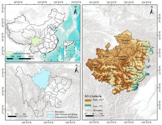
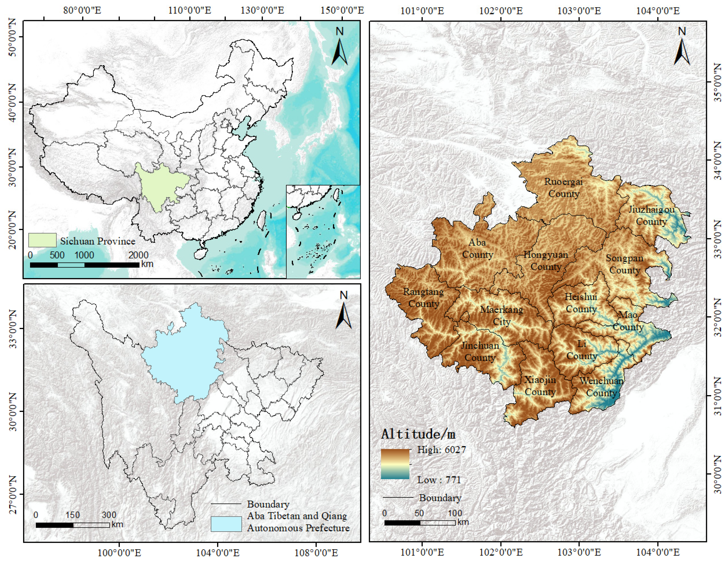
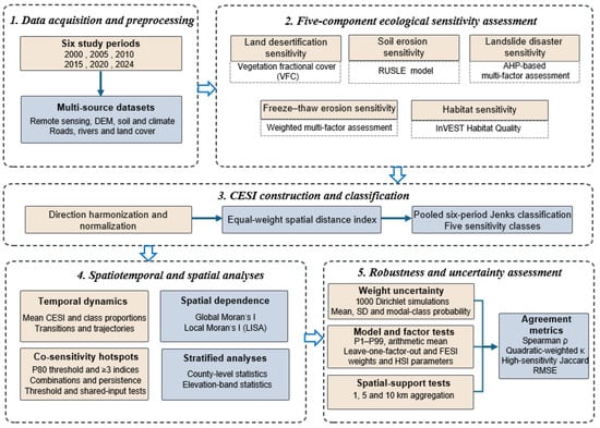
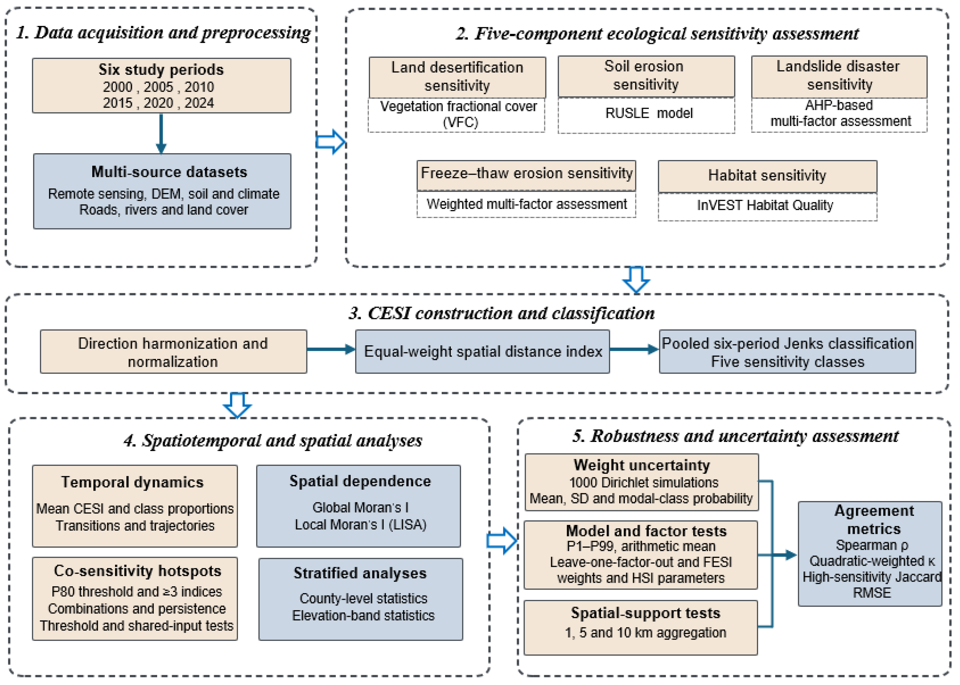
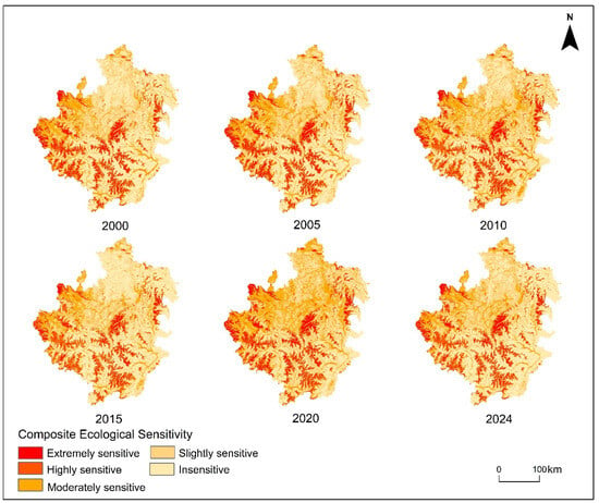
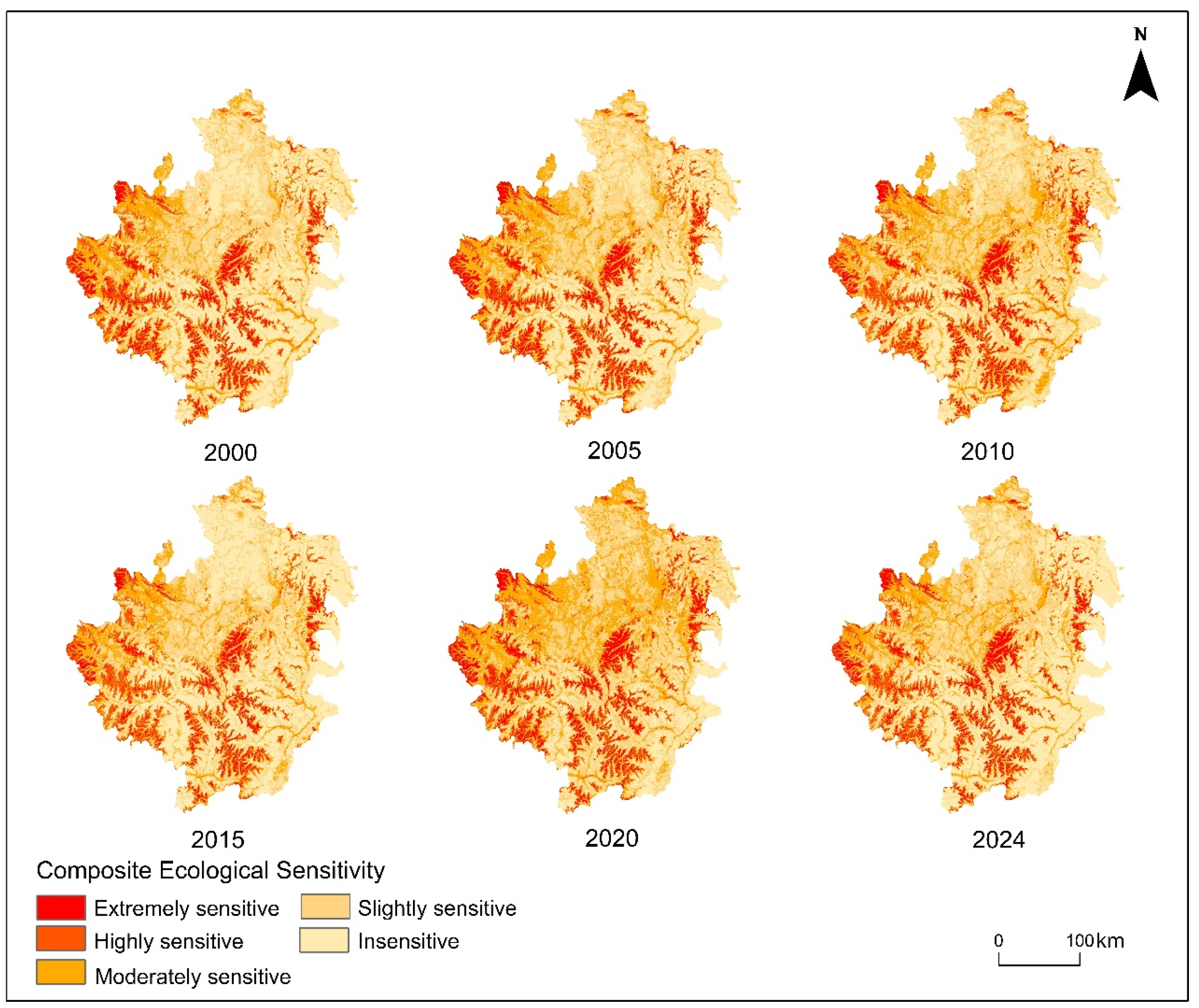
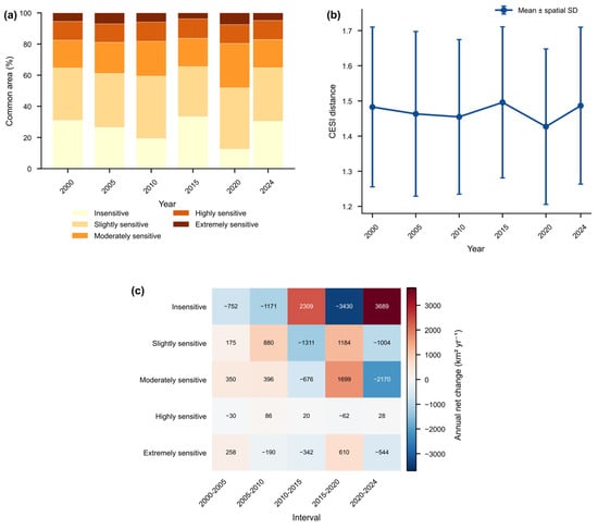
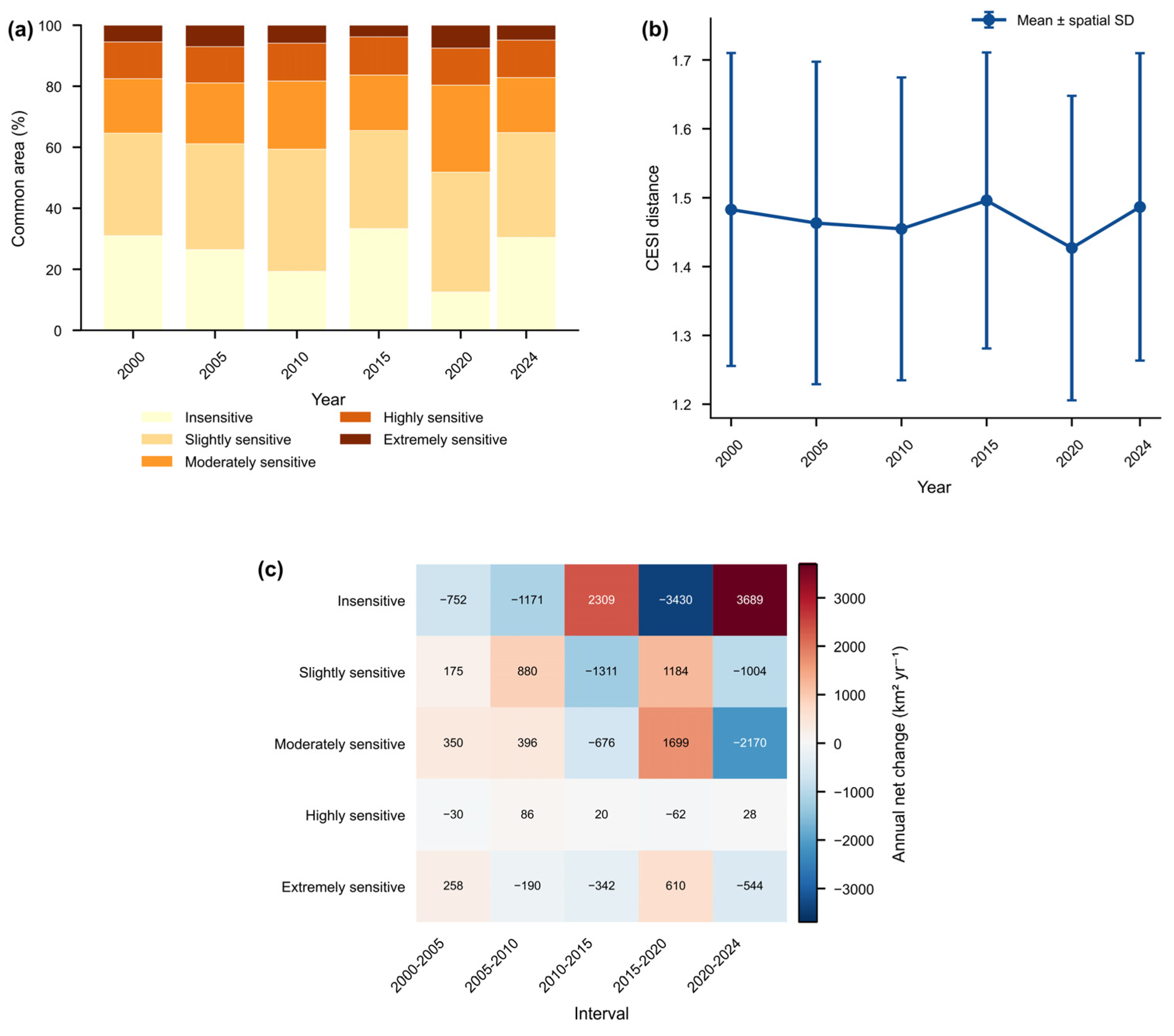
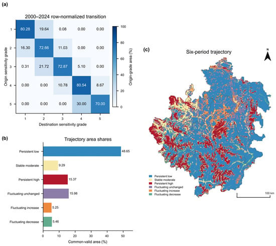
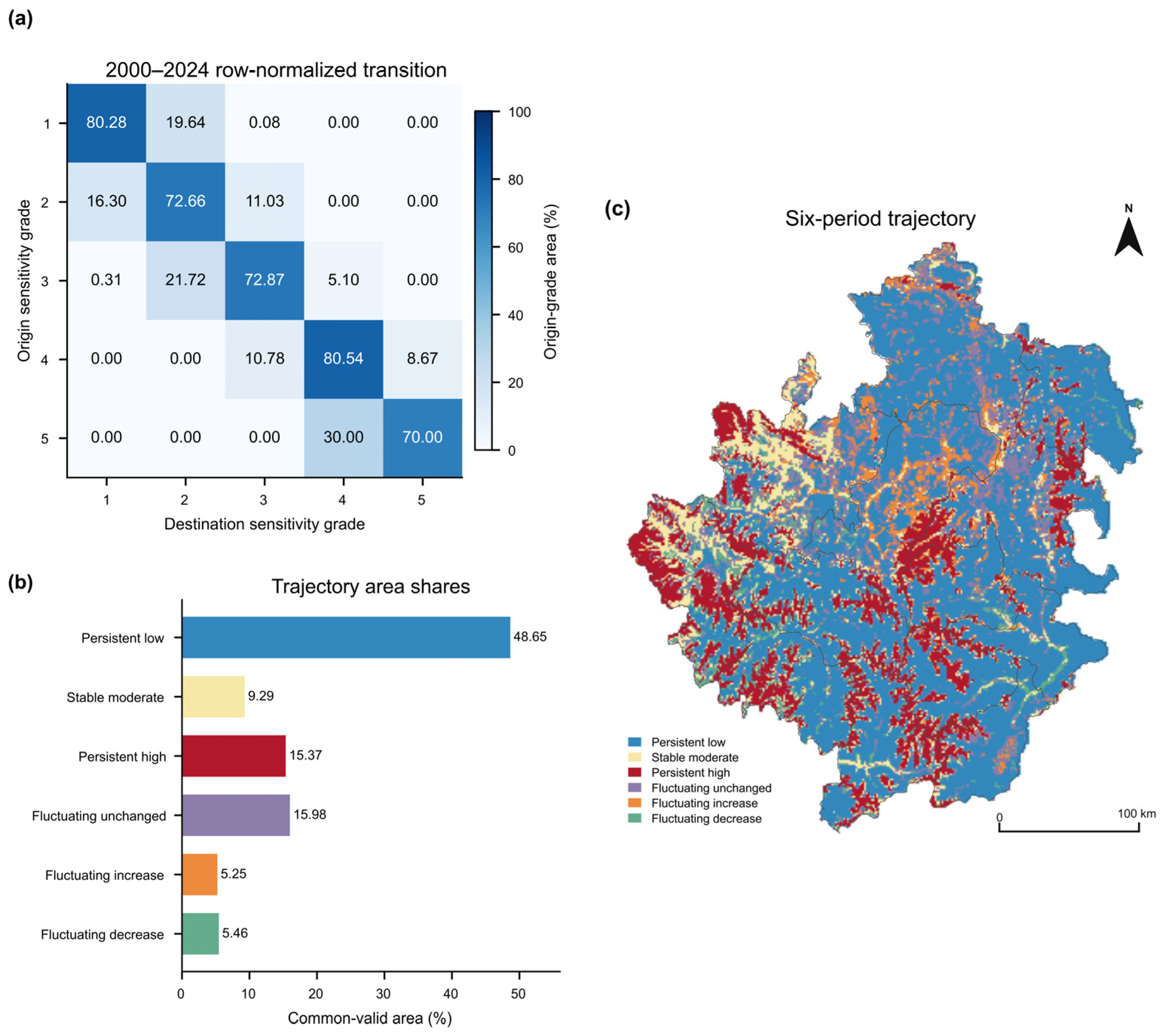
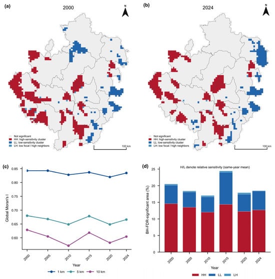
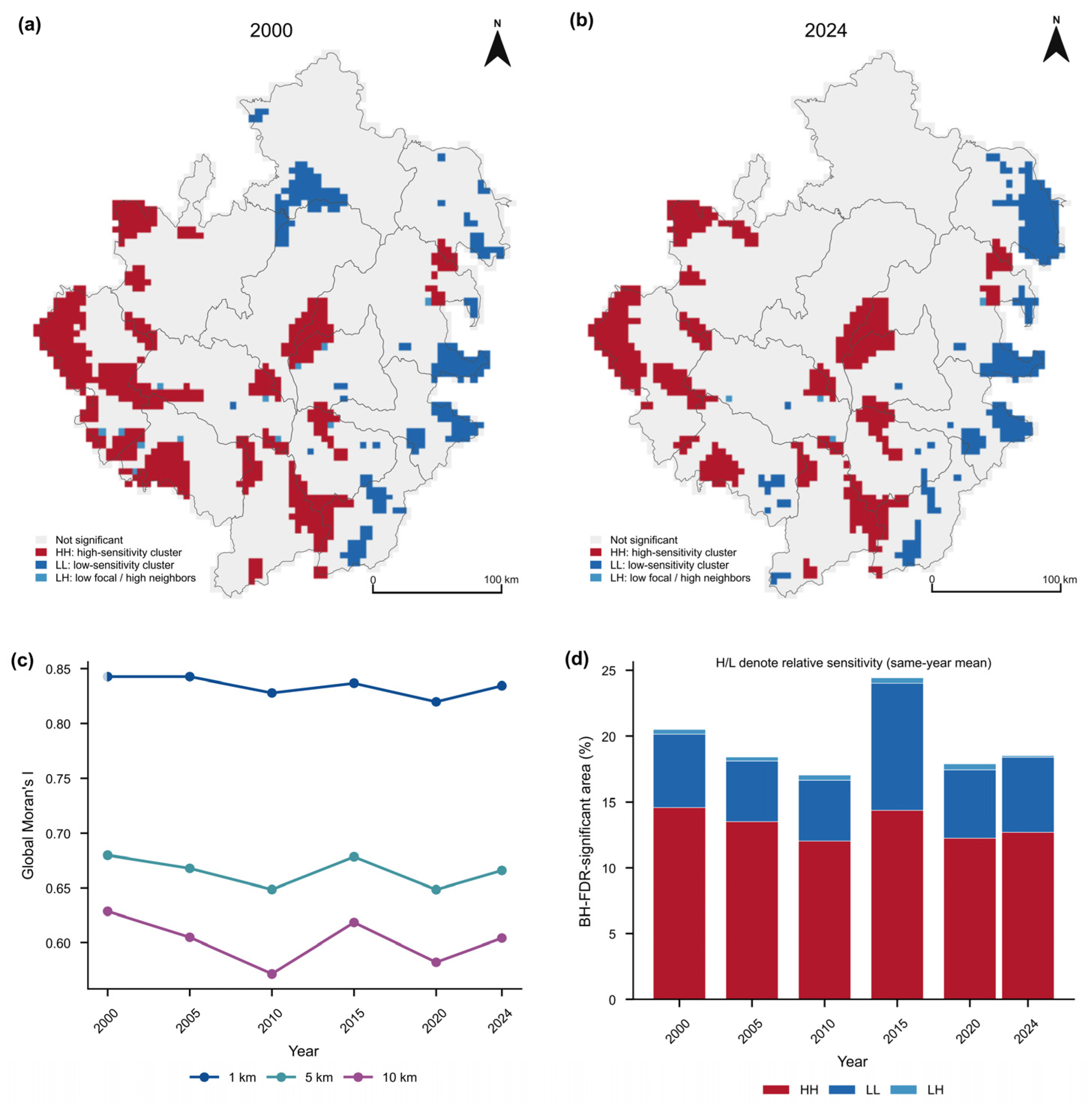
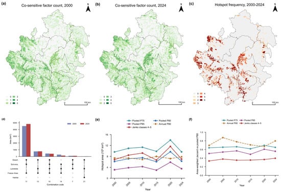
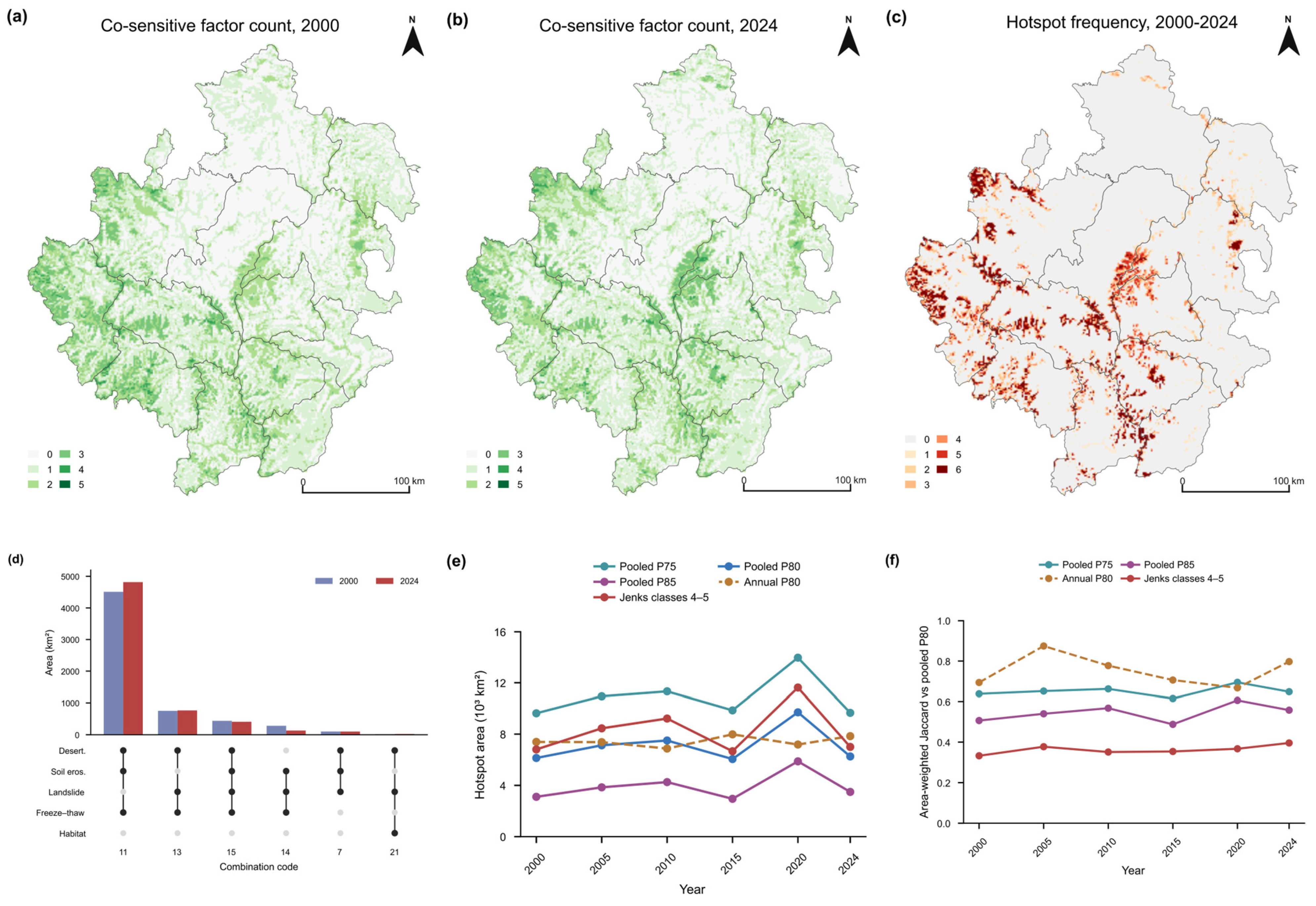
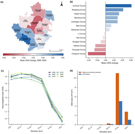
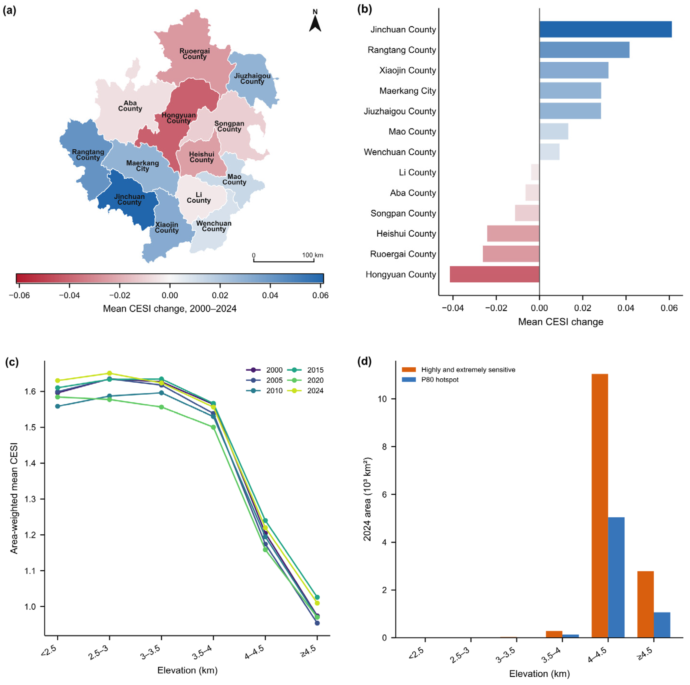
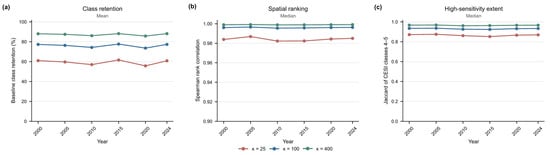
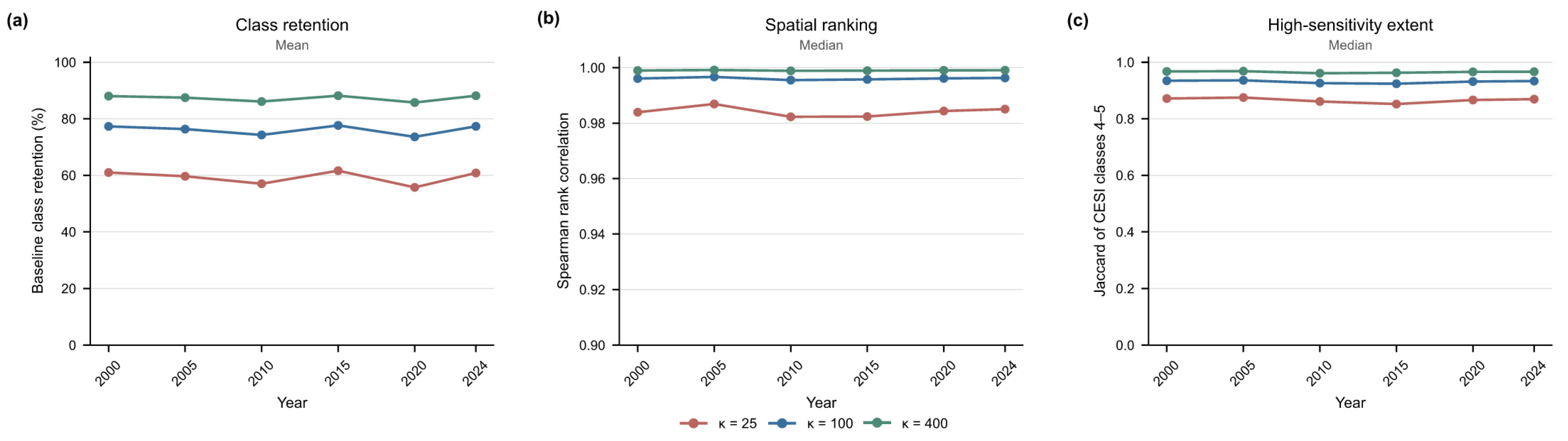
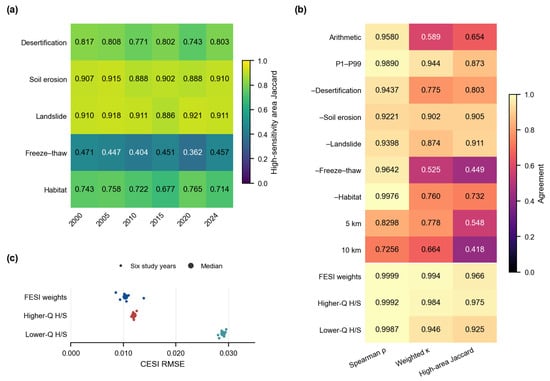
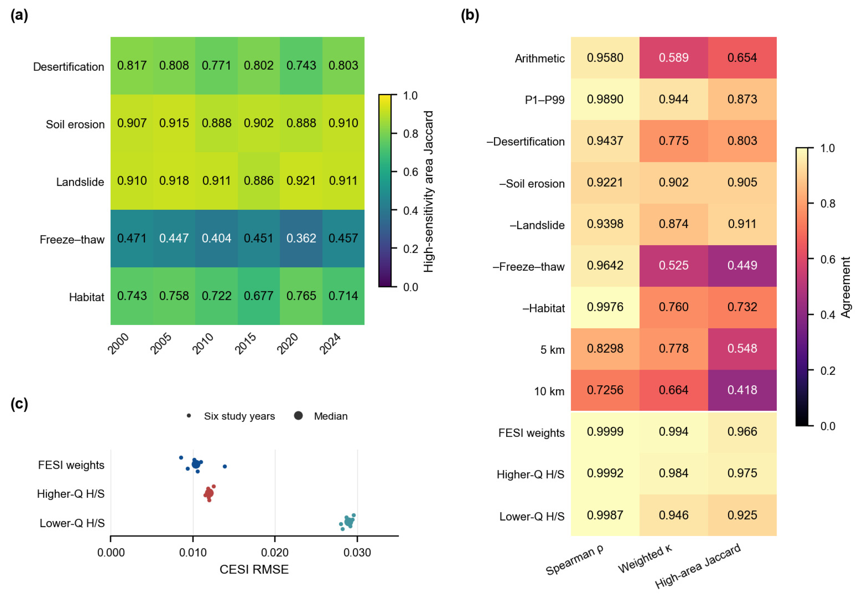

Disclaimer/Publisher’s Note: The statements, opinions and data contained in all publications are solely those of the individual author(s) and contributor(s) and not of MDPI and/or the editor(s). MDPI and/or the editor(s) disclaim responsibility for any injury to people or property resulting from any ideas, methods, instructions or products referred to in the content. |
© 2026 by the authors. Licensee MDPI, Basel, Switzerland. This article is an open access article distributed under the terms and conditions of the Creative Commons Attribution (CC BY) license.