An Intelligent Blind Feature Clustering Framework for Automated Modal Discrimination of Concrete Dams

Abstract

Automated modal identification of concrete dams under ambient excitation remains challenging because spurious modes arising from non-white excitation, noise, and algorithmic artifacts can obscure physical modes and complicate automated discrimination. Conventional approaches, such as stabilization diagram interpretation in stochastic subspace identification, still require extensive user expertise. This study proposes an intelligent blind feature clustering framework built on a recently developed blind subspace identification method that separates modal responses without stabilization diagrams. In this framework, an improved differential evolution algorithm integrated with K-means clustering searches for the optimal clustering scheme in the feature space defined by modal feature indices extracted from the separated modal responses. Compared with conventional approaches, the proposed framework avoids subjective threshold selection and manual pole picking, thereby facilitating automated modal discrimination. The framework was applied to a large concrete arch-gravity dam. Five physical modes were identified, and the remaining modes were classified as spurious. The identified modal parameters agree well with those obtained by SSI-COV, FDD, and FEM, and the proposed clustering yields more stable results than conventional K-means with random initialization. In this case study, the proposed framework achieved automated modal discrimination without constructing or interpreting stabilization diagrams, while reducing reliance on expert intervention. These results suggest a promising approach for automated modal identification and long-term modal monitoring of concrete dams.

1. Introduction

Concrete dams have become the dominant structural type for large and medium-sized reservoirs due to their inherent safety, reliability, and excellent durability [1]. However, these structures are typically situated in mountainous gorge regions and are continuously subjected to multiple environmental and operational loads, such as water pressure and temperature variations [2,3]. As service age increase, structural damage and material degradation may gradually develop [4]. Given the catastrophic consequences associated with dam failures, real-time monitoring and continuous safety assessment of dams are of critical importance [5,6].

Current safety monitoring of concrete dams generally relies on static measurements, with deformation being the most representative indicator [7,8,9,10]. Static measurements primarily focus on the phenomenological description of dam behavior [11]. However, given the multiplicity of influencing factors and the complexity of their underlying mechanisms, static monitoring exhibits inherent limitations in capturing the intrinsic physical and mechanical properties of concrete dams [12,13]. In contrast, the vibration responses of concrete dams encapsulate multimodal structural state information, which can more effectively characterize the evolution of their physical and mechanical properties [14,15,16]. This information is conveyed by modal parameters, including natural frequencies, modal damping ratios, and mode shapes. A concrete dam in operation is under ambient excitations from microtremors, flow-induced pulsations, powerhouse operations, and crest traffic [17]. These excitations typically possess broadband spectrum characteristics similar to white noise and can excite structural modes within a certain frequency range [18]. Therefore, if modal parameters of concrete dams can be reliably identified in an automated manner from ambient vibration monitoring data, structural damage can be detected and early warnings issued timely, enabling a more comprehensive assessment of the dam’s safety state [19,20,21].

In practice, however, ambient excitation rarely satisfies the white noise assumption perfectly. This deviation can be conceptually represented as a load filter between idealized white noise input and the actual excitation acting on the structure [22]. Consequently, measured output signals may contain frequency components that do not originate from the structural modes [23]. Moreover, operational modal analysis algorithms such as stochastic subspace identification (SSI) can produce additional spurious computational modes due to factors like model order redundancy [24]. Furthermore, periodic excitations and noise interference can introduce spurious harmonics and noise modes into the identified results [25]. All these non-physical components manifest as spurious modes in the subsequent modal identification. To enable real-time monitoring of modal parameters, intelligent methods are required to automatically discriminate physical modes from spurious modes, thereby replacing the screening process that relies on expert experience [26]. This task is particularly challenging for concrete dams. The ambient excitations acting on such structures are often non-stationary and of low amplitude [27]. Moreover, the dam-reservoir-foundation system is highly complex [28]. These factors give rise to closely spaced or weakly excited modes that can easily be masked by spurious modes [29].

The existing studies on automated modal discrimination have predominantly relied on SSI or frequency domain decomposition (FDD). For FDD, Brincker et al. [30] introduced discrimination indicators to automated identify modal peaks in the first singular value spectra. Magalhães et al. [31] refined these discrimination indicators by introducing a statistical criterion. However, difficulties remain in threshold selection and automated identification of physical modes. Rainieri et al. [32] partially mitigated these shortcomings by applying modal assurance criterion sequences to identify the mode bandwidth before modal parameter extraction. Compared with FDD, SSI offers higher accuracy and better robustness, and is therefore more commonly adopted in practical applications. Peeters and De Roeck [33] established the foundational framework for modal discrimination of SSI with stabilization diagram by defining stability tolerances across adjacent model orders and selecting the stable poles. However, stabilization diagrams are often ambiguous, demanding extensive user interaction and expert judgment to resolve physical modes. To overcome this limitation, numerous studies have focused on enhancing diagram clarity and introducing clustering techniques for automated modal discrimination. Magalhães et al. [34] adopted hierarchical clustering to group physical poles, automatically accepting clusters exceeding a predefined size as physical modes. Reynders et al. [35] proposed a fully automated three-stage clustering approach with multiple validation criteria to progressively interpret the stabilization diagram. Ubertini et al. [36] developed an iterative clustering approach that simultaneously considers model order and the number of block rows in the block Hankel matrix. Cabboi et al. [37] proposed a self-adaptable threshold clustering strategy and introduced a modal complexity index to filter out spurious modes prior to clustering. Li et al. [38] performed the DBSCAN clustering algorithm to interpret the stabilization diagram and applied to Dagangshan arch dam. Li et al. [39] combined SSI, sparrow search algorithm and K-means algorithm to automatically identify the physical modes of a high arch dam under seismic excitation. Wu et al. [40] developed a hybrid clustering algorithm combing density peaks clustering with a shared nearest neighbor approach to group physical modes and applied to a small-scale arch dam. Li et al. [41] combined the adaptive multivariate variational mode decomposition, the three-dimensional stabilization diagram, and an improved fuzzy K-means clustering algorithm to distinguish physical modes. The method was validated using a physical arch dam model and a prototype arch dam. Although clustering-based methods can, to a certain extent, facilitate automated modal discrimination within the SSI framework, they do not fundamentally overcome the difficulty of distinguishing physical poles in stabilization diagrams. This challenge is particularly pronounced for large dams, which are massive structures characterized by complex operating conditions and relatively weak excitation [42]. In such cases, the poles in stabilization diagrams are often chaotically distributed, rendering the clustered results unreliable and inaccurate. Therefore, it is imperative to develop new automated modal discrimination approaches that can provide a solid foundation for the automated monitoring of modal parameters in concrete dams.

In previous studies by the authors, a blind subspace identification method was proposed, in which blind source separation is integrated into the stochastic subspace identification framework [43,44]. This method enables effective separation of modal responses from ambient vibration measurements and achieves high-accuracy modal parameter identification without constructing or interpreting stabilization diagrams. This provides a reliable foundation for automated operational modal analysis of concrete dams. Nevertheless, the automated modal discrimination has yet to be fully achieved. To address this challenge, the present study proposes an intelligent blind feature clustering framework built upon the previously developed blind subspace identification method. In this framework, three modal feature indices are extracted from the separated modal responses. An improved differential evolution algorithm is integrated with K-means clustering to search for the optimal clustering scheme in the feature space, thereby enabling automated modal discrimination without reliance on stabilization diagrams or expert intervention. The proposed method is validated using ambient vibration data from a large concrete arch-gravity dam, demonstrating its effectiveness and practical applicability.

2. Methodology

2.1. Blind Source Separation for Modal Identification

The fundamental principle of modal identification via blind subspace identification is to separate the modal responses using blind source separation (BSS), and then to identify the modal parameters from these modal responses parametrically.

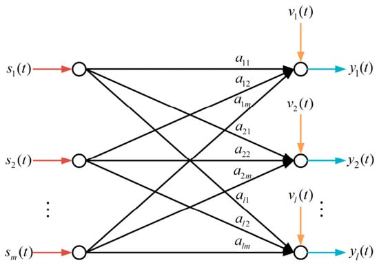
BSS is primarily employed to process multiple-input multiple-output systems. Consider that observed signals $y(t)={[y_1(t),y_2(t),\cdots ,y_l(t)]}^T$ acquired by l channel sensors are mixtures of m source components $s(t)={[s_1(t),s_2(t),\cdots ,s_m(t)]}^T$. Accounting for additive noise v(t), the linear instantaneous mixing BSS model (Figure 1) can be formulated as:

y(t) = As(t) + v(t)

(1)

where A is the mixing matrix.

Figure 1. Schematic of the linear instantaneous BSS model.

The objective of BSS is to find the de-mixing matrix B = A^† and source components s(t) using the observed signals y(t) by characterizing the sources, considered as the following de-mixing model:

s(t) = By(t)

(2)

To reliably recover the m source components, acquiring an adequate number of observations l is a fundamental prerequisite. This necessitates that l ≥ m and that the mixing matrix A is of rank m. Furthermore, the simultaneous estimation of the de-mixing matrix B and the source components s(t) introduces scaling and permutation ambiguities. The amplitude of each source component is typically fixed by constraining the variance of sources to unity, namely R_s(0) = E{ss^H} = I.

Building on the abovementioned BSS model, the rationale for applying BSS to modal analysis lies in the profound structural correspondence between the two fields. In structural dynamics, the vibration response of a structural system can be expressed through the modal superposition principle as:

y(t) = Ψq(t)

(3)

where Ψ is the matrix of mode shapes, and q(t) is the vector of modal responses. This formulation is mathematically isomorphic to the noiseless linear instantaneous mixing BSS model. Under this equivalence, the mixing matrix A corresponds to the modal matrix Φ, while the source components s(t) map directly onto the modal responses. Once the mixing matrix is recovered, the modal responses are separated and modal parameters can be analyzed.

For systems with general viscous damping, the mode shapes and the associated modal responses manifest as complex conjugate pairs, which can be respectively expressed as Ψ = [Φ,Φ^∗] and $q(t)={[q_r^T(t),q_r^H(t)]}^T$. The conjugate duplication can be eliminated by converting the modal superposition principle into its analytic signal form [45] as:

$$\tilde{y}(t)=\Phi {\tilde{q}}_r(t)$$

(4)

where $\tilde{y}(t)$ and ${\tilde{q}}_r(t)$ denote the analytic signal forms of y(t) and q_r(t), respectively, expressed as:

$$\tilde{y}(t)=y(t)+\mathrm{i}\widehat{y}(t), {\tilde{q}}_r(t)=q_r(t)+\mathrm{i}{\widehat{q}}_r(t)$$

(5)

where $\widehat{y}(t)$ and ${\widehat{q}}_r(t)$ denote the Hilbert transforms of y(t) and q_r(t), respectively, and i denotes the imaginary unit. $\widehat{y}(t)$ is calculated as:

$$\widehat{y}(t)={\displaystyle \frac{1}{\pi }}{\displaystyle {\displaystyle \underset{-\infty }{\overset{\infty }{\int }}}\frac{y(t)}{t-\tau }\mathit{d\tau }}$$

(6)

Once the mixture is expressed in this compact complex-valued form, BSS can be directly performed on the analytic signals to recover the modal responses.

2.2. Overview of Blind Subspace Identification

The blind subspace identification procedure comprises modal response separation and modal parameter identification. For the modal response separation, the second-order blind identification (SOBI) algorithm in analytic form is adopted. SOBI separates source components that are spatially uncorrelated and individually temporally correlated with distinct autocorrelation structures, which aligns naturally with structural modal properties.

Three principal stages are involved in the estimation: windowing, whitening, and de-mixing. Windowing is first applied on the analytic observation vector by tapering the signal with a smooth window function (such as Gaussian, Hanning, or Hamming) to gradually attenuate the signal near the boundaries, which limits spectral leakage and reduces truncation artifacts, making the spectrum more suitable for further processing. Additionally, windowing helps keep the extracted source components from becoming excessively uncorrelated across time shifts relative to the actual modal responses [46].

Whitening is then performed on the windowed analytic observation vector $\tilde{y}(t)$ by multiplying it with a whitening matrix W to obtain the whitened signals z(t) as:

$$z(t)=W\tilde{y}(t)$$

(7)

The whitening matrix W is typically obtained from the eigenvalue decomposition of the windowed analytic observation vector’s zero-lag covariance matrix $R_y(0)=E\left\{\tilde{y}{\tilde{y}}^H\right\}$, expressed as:

W = D^−1/2E^H

(8)

with D and E being the eigenvectors and eigenvalues of the zero-lag covariance matrix as:

R_y(0) = EDE^H

(9)

so that the whitened signals z(t) has an identity covariance matrix, i.e., R_z(0) = WR_y(0)W^H = (D^−1/2E^H)(EDE^H)(ED^−1/2) = I, removing all instantaneous cross-correlations and equalizing the variances across channels, yielding spatially uncorrelated signals with unit variance. Furthermore, whitening ensures that the subsequent de-mixing focuses solely on the temporal autocorrelation structures of the sources, preventing unequal channel scaling or spurious instantaneous correlations from biasing the modal identification. It also reduces the original BSS problem from estimating an unconstrained mixing matrix A to finding a unitary matrix U, inherently enforcing a unitary constraint, as R_z(0) = WAR_s(0)A^HW^H = I with R_s(0) = I, forcing U = WA to be unitary.

After whitening, the de-mixing is accomplished via joint approximate diagonalization (JAD) of a set of time-lagged covariance matrices R_z(τ) = E{z(t)z(t + τ)^H}. This yields a unitary matrix U that maximally decorrelates the sources across multiple time lags τ. The JAD is typically achieved by minimizing the off-diagonal squared norm as:

$${\displaystyle \underset{U^{H}U=I}{\min }}{\displaystyle \sum _{\tau =1}^p{‖\mathrm{off}(U^H{R}_z(\tau )U)‖}_F^2}$$

(10)

where off(·) denotes the operator that extracts the off-diagonal part of a matrix, and ‖·‖_F is the Frobenius norm. The optimization is typically executed through an iterative Jacobi-like procedure. The unitary matrix U is constructed as a product of a sequence of Givens rotations, where each rotation targets a specific pair of coordinates. For each pair (r,s), the rotation matrix is identical to the identity matrix except for the elements at the intersections of the rth and sth rows and columns, the rotation blocks extracted from the (r,s) rows and columns are given by:

$$G(r,s,\theta ,\varphi )=\left[\begin{array}{cc}\cos \theta & e^{\mathrm{i}\varphi }\sin \theta \\ -e^{-\mathrm{i}\varphi }\sin \theta & \cos \theta \end{array}\right]$$

(11)

where θ and ϕ are rotation angle and phase angle, respectively. The minimization problem can be shown to be equivalent to maximizing the following quadratic form [47]:

g(θ,ϕ) = u^TRe(Q^HQ)u

(12)

where u and Q are:

$$\begin{array}{l}u={[\cos 2\theta ,-\sin 2\theta \cos \varphi ,-\sin 2\theta \sin \varphi ]}^T\\ Q={[{[a_1-d_1,b_1+c_1,\mathrm{i}(c_1-b_1)]}^T,\cdots ,{[a_{\tau }-d_{\tau },b_{\tau }+c_{\tau },\mathrm{i}(c_{\tau }-b_{\tau })]}^T]}^T\end{array}$$

(13)

where a_k, b_k, c_k, and d_k are the kth time-lagged covariance matrix at the intersections of rows r, s and columns r, s, and Q^HQ is Hermitian. The parameters θ and ϕ are identified by taking u as the unit-norm eigenvector corresponding to the largest eigenvalue of Re(Q^HQ). The unitary matrix U, formed by successively right-multiplying all Givens rotation matrices, then yields the analytic modal responses directly as:

$${\tilde{q}}_r(t)=U^{H}W\tilde{y}(t)$$

(14)

In order to mitigate the susceptibility to cross-modal leakage that undermine the normally used single-degree-of-freedom (SDOF) techniques when applied to the estimated modal responses [48], the authors proposed a multi-degree-of-freedom (MDOF) identification framework that simultaneously identifies all modal parameters [42,43,44]. The method is build upon the following parametric system model in discrete-time state-space form [42]:

$$\begin{array}{l}{\tilde{z}}_{k+1}={\Lambda }_d{\tilde{z}}_k+w_k\\ \mathrm{Re}(q_k)=V_d{\tilde{z}}_k+v_k\end{array}$$

(15)

where q_k = q(kΔt), ${\tilde{z}}_k$ is the state vector, w_k and v_k are the input and output noise vectors, and Λ_d and V_d are the state matrix and output matrix, respectively. Λ_d is given by:

$${\Lambda }_d=\left[\begin{array}{cc}{e}^{\Lambda \Delta t}& 0\\ 0& e^{{\Lambda }^{\ast }\Delta t}\end{array}\right]$$

(16)

where Λ = diag(λ₁, λ₂, ⋯, λ_N), λ_j is the jth eigenvalue of the N DOF structural system, expressed as:

$${\lambda }_j=-{\xi }_j{\omega }_j+\mathrm{i}{\omega }_j\sqrt{1-{\xi }_j^2}$$

(17)

where ω_j and ξ_j are the natural circular frequency and damping ratio associated with the jth mode.

Based on the parametric system model given in Equation (15), the natural frequencies f_j = ω_j/2π and damping ratios ξ_j can be estimated using an SSI-like MDOF approach as follows [44].

From the estimated modal responses Re(q_k), the output covariance matrices $R_q(\tau )=\mathrm{E}\{\mathrm{Re}(q_k)\mathrm{Re}(q_k^T)\}$ are estimated for a set of time lags τ = 1, ⋯, 2i − 1 and then assembled into the following block Toeplitz matrix:

$$T=\left[\begin{array}{cccc}{R}_q(i)& R_q(i-1)& \cdots & R_q(1)\\ R_q(i+1)& R_q(i)& \cdots & R_q(2)\\ ⋮& ⋮& \ddots & ⋮\\ R_q(2i-1)& R_q(2i-2)& \cdots & R_q(i)\end{array}\right]$$

(18)

Applying the singular value decomposition (SVD) to block Toeplitz matrix T produces the following results:

$$T=U_1{S}_1{V}_1^T$$

(19)

where U₁ and V₁ are truncated orthogonal matrices comprising the left and right singular vectors, respectively, and S₁ is a truncated diagonal matrix containing the singular values in descending order. The observability matrix is then obtained as:

$$O=U_1{S}_1^{1/2}$$

(20)

From the observation matrix O, the state matrix Λ_d can be estimated using a shift-invariance property as:

Λ_d = O(1:l(i − 1),:)^†O(l + 1:li,:)

(21)

where † denotes the Moore–Penrose pseudoinverse. The natural frequencies f_j and damping ratios ξ_j are then identified according to Equation (17) as:

$$f_j={\displaystyle \frac{1}{2\pi }}\sqrt{\mathrm{Re}{({\lambda }_j)}^2+\mathrm{Im}{({\lambda }_j)}^2}, {\xi }_j={\displaystyle \frac{-\mathrm{Re}({\lambda }_j)}{2\pi f_j}}$$

(22)

2.3. Feature Clustering Integrating K-Means Clustering and Differential Evolution

Automated discrimination of physical modes from spurious modes is a prerequisite for applying blind subspace identification to real-time monitoring of dam modal parameters. Toward this end, a blind feature clustering method is developed, where K-means clustering is integrated with differential evolution to partition the identified modes into physical and spurious clusters.

For the jth modal response separated through blind subspace identification, a set of modal feature indices is first constructed to characterize its physical plausibility from three complementary perspectives, namely the spectral concentration, temporal regularity, and spectral flatness. The corresponding indices, i.e., the Spectral Variance (SV), Length of Envelope (LE), and Spectral Entropy (SE), are detailed below.

• Spectral Variance (SV);

The Spectral Variance is adopted to quantify the spectral concentration of the modal response. For a physical mode, the spectral energy is highly concentrated around a modal frequency. In contrast, a spurious mode typically exhibits a broader spectrum.

Accordingly, the SV index is computed as the normalized second central moment of the power spectral density within a specified frequency band centered at the modal frequency, defined by:

$$S{V}_j={\displaystyle \frac{{\displaystyle \sum _{k=1}^{N_f}(f_k}-{\overline{f}}_j{)}^2{S}_j(f_k)}{{\displaystyle \sum _{k=1}^{N_f}{S}_j(f_k)}}}$$

(23)

where S_j(f_k) denotes the normalized power spectral density of the jth modal responses at the kth discrete frequency f_k, N_f is the number of frequency samples within the selected band, and ${\overline{f}}_j$ denotes the barycentric frequency, defined by:

$${\overline{f}}_j={\displaystyle \sum _{k=1}^{N_f}{f}_k{S}_j(f_k)}$$

(24)

A lower SV value indicates a higher degree of spectral concentration and hence a stronger physical plausibility.

2.

Length of Envelope (LE);

The Length of Envelope is introduced to characterize the temporal regularity of the modal response envelope. For a physical mode under ambient excitation, the modal response approximates a narrowband Gaussian process. Its envelope exhibits regular fluctuations, yielding a relatively short trajectory over a given time window. In contrast, a spurious mode normally produces an irregular envelope with more frequent and abrupt fluctuations, resulting in a longer trajectory.

The LE index is defined as the arc length of the Hilbert transform envelope computed over a specified time window, given by:

$$L{E}_j={\displaystyle \sum _{k=2}^{N_t}\sqrt{{(\left|{\tilde{q}}_{j,k}\right|-\left|{\tilde{q}}_{j,k-1}\right|)}^2+{(t_k-t_{k-1})}^2}}$$

(25)

where ${\tilde{q}}_{j,k}$ is the analytic signal of the jth modal response.

A lower LE value indicates a more regular temporal structure and serves as a positive indicator of physical plausibility.

3.

Spectral Entropy (SE).

The Spectral Entropy is employed to evaluate the spectral flatness of the modal response. A physical mode, characterized by a dominant spectral peak, yields a highly non-uniform power spectrum and consequently low entropy. In contrast, a spurious mode typically contains multiple frequency components that yield a flatter spectrum and consequently higher entropy.

The SE index is derived from the concept of information entropy. By treating the normalized power spectral density within the frequency band of interest as a probability-like distribution, the SE index is defined as:

$$S{E}_j=-{\displaystyle \sum _{k=2}^{N_t}{S}_j(f_k)\ln }{S}_j(f_k)$$

(26)

A lower SE value reflects the spectral simplicity characteristic of a genuine physical mode, whereas a higher SE value suggests the presence of spurious content.

For each identified modal response, these indices are normalized and assembled into a feature vector $x_j={[S{V}_j,L{E}_j,S{E}_j]}^T$. It should be noted that the assumption that physical modes exhibit lower feature values represents only an idealized case and may not always hold in practice, especially in complex practical applications involving weakly excited structural modes or narrowband interference. Therefore, the subsequent modal discrimination procedure cannot rely on absolute criterions, but instead achieved through the feature clustering described below.

Let $\mathcal{X}$ = {x₁, x₂, ⋯, x_l} denote the set of feature points extracted from L identified modal responses, which serve as the input to the subsequent feature clustering procedure. The objective of clustering is to partition these vectors into two clusters $\mathcal{S}$₁ and $\mathcal{S}$₂, corresponding to physical modes and spurious modes, respectively. This two-cluster partition is adopted because spurious responses are generally expected to be present in the separation results, since the number of measurement channels is typically larger than the number of identifiable modes, as discussed earlier.

The optimal partition $\{{\mathcal{S}}_1^{\ast },{\mathcal{S}}_2^{\ast }\}$ is obtained by minimizing the within-cluster sum of square distances between each feature point and its nearest cluster centroid, i.e.,

$$\{{\mathcal{S}}_1^{\ast },{\mathcal{S}}_2^{\ast }\}={\displaystyle \underset{\{{\mathcal{S}}_1,{\mathcal{S}}_2\}}{\arg \min }}{\displaystyle \sum _{s=1}^2{\displaystyle \sum _{x_j\in {\mathcal{S}}_s}{‖x_j-c_s‖}^2}}$$

(27)

where ‖·‖ denotes the Euclidean norm, and c_s denotes the centroid of cluster $\mathcal{S}$_s, defined as:

$$c_s={\displaystyle \frac{1}{\left|{\mathcal{S}}_s\right|}}{\displaystyle \sum _{x_j\in {\mathcal{S}}_s}{x}_j}$$

(28)

In the conventional K-means algorithm, the cluster centroids are initialized randomly and updated iteratively through an expectation maximization procedure. However, the final solution is highly sensitive to the initial guess and may converge to a local optimum, and its performance can deteriorate when outlier or weakly conditioned components are present, or when the sample distribution is unbalanced. To overcome this limitation, the differential evolution (DE) algorithm [49] is integrated into the clustering framework to search for the optimal cluster centroids in the feature space.

In the DE-based clustering procedure, each candidate solution encodes a pair of cluster centroids, represented as a six-dimensional vector $v={[c_1^T,c_2^T]}^T$. The fitness function of each candidate solution is evaluated as:

$$\mathit{fit}(v)={\displaystyle {\displaystyle \sum _{s=1}^2}{\displaystyle \sum _{x_j\in {\mathcal{S}}_s}{‖x_j-c_s‖}^2}}$$

(29)

The DE algorithm operates as follows. An initial population $\{v_1^0,v_2^0,\dots ,v_{N_p}^0\}$ is generated randomly within the feature space. For each individual, the six components are generated uniformly within the range [0,1] to bring features with different units and scales into a unified analysis framework. The algorithm evolves the NP solutions through repeated cycles of mutation, crossover, and selection, as detailed below.

• Mutation

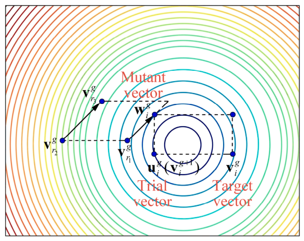
At each generation g, for each target vector $v_i^g$, a mutant vector $w_i^g$ is generated according to the mutation strategy:

$$w_i^g=v_{r_1}^g+F(v_{r_3}^g-v_{r_2}^g)$$

(30)

where r₁, r₂, r₃ are mutually distinct indices randomly selected from {1, 2, …, NP}\{i}, and F ∈ [0,1] is the scaling factor that controls the influence of the difference vector on the mutant vector.

It should be noted that the mutant vector may exceed the feasible bounds, thereby producing an invalid solution. Specifically, the mth component $w_{\mathit{im}}^g$ of the mutant vector $w_i^g$ may no longer fall within the range [0,1]. For any out-of-bound component, random reinitialization is performed to ensure a feasible solution.

B.

Crossover

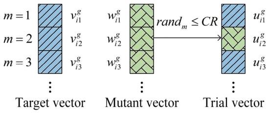
To enhance population diversity, for each target vector $v_i^g$, a trial vector $u_i^g$ is generated through binomial crossover between $v_i^g$ and the corresponding mutant vector $w_i^g$. The mth component of the trial vector is given by:

$$u_{\mathit{im}}^g=\left\{\begin{array}{c}{w}_{\mathit{im}}^g\\ v_{\mathit{im}}^g\end{array}\right.\begin{array}{l}\hfill \end{array}\begin{array}{c}{\mathit{rand}}_m\le \mathit{CR} \mathrm{or} m=m_{\mathit{rand}}\\ {\mathit{rand}}_m>\mathit{CR} \mathrm{and} m\ne m_{\mathit{rand}}\end{array}$$

(31)

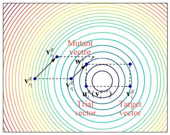
where rand_m is a uniformly distributed random number in range [0,1], CR ∈ [0,1) is the crossover rate, which determines the likelihood that a given component of the trial vector is inherited from the mutant vector, and m_rand is a randomly selected integer in the range [1,6] that ensures the trial vector inherits at least one component from the mutant vector. The crossover operator is illustrated in Figure 2.

Figure 2. Schematic of crossover operation in differential evolution.

C.

Selection

The selection operation compares the fitness function of the trial vector and the target vector. If the trial vector yields less or equal fitness function value, it replaces the target vector in the next generation. Otherwise, the target vector is retained. After selection, the updated target vector $v_i^{g+1}$ is given by:

$$v_i^{g+1}=\left\{\begin{array}{c}{u}_i^g\\ v_i^g\end{array}\right.\begin{array}{l}\hfill \end{array}\begin{array}{c}\mathit{fit}(u_i^g)\le \mathit{fit}(v_i^g)\\ \mathit{fit}(u_i^g)>\mathit{fit}(v_i^g)\end{array}$$

(32)

The core operators of the differential evolution algorithm are illustrated in Figure 3.

Figure 3. Schematic of core operators of the differential evolution algorithm.

Consequently, the best fitness function value of the population is guaranteed to be monotonically non-increasing as the evolution proceeds. The evolution process continues until a prescribed maximum number of generations g_max is reached or the improvement in the best fitness value falls below a predefined tolerance ε. Upon convergence, the best individual in the final population is decoded to obtain the optimal cluster centroids $c_1^{\ast }$ and $c_2^{\ast }$.

With the optimal cluster centroids determined, each feature vector x_j is assigned to the cluster whose centroid is nearest, yielding the final partition $\{{\mathcal{S}}_1^{\ast },{\mathcal{S}}_2^{\ast }\}$. The cluster with the lower average feature values is identified as the physical mode cluster, while the other is regarded as the spurious mode cluster. This completes the automated discrimination procedure.

The performance of the DE algorithm depends heavily on the settings of its control parameters. As can be seen from the basic procedure of DE, three parameters need to be specified in advance: the population size NP, the scaling factor F, and the crossover rate CR. Among them, the latter two control parameters exert a significant influence on the global search capability and convergence speed of the algorithm. Inappropriate parameter settings may cause the algorithm to become trapped in local optima, leading to premature convergence, or may result in slow convergence with insufficient accuracy of the global optimum. As indicated by Equation (30), a large F imposes a stronger perturbation on the mutant vector $w_i^g$, which enhances population diversity and increases the probability of locating the global optimum. However, the algorithm then tends toward random search, resulting in relatively low convergence speed and solution accuracy. Conversely, a small F imposes a weaker perturbation, enabling more refined local search and faster convergence, but at the risk of becoming trapped in local optima and exhibiting premature convergence. As indicated by Equation (31), a large CR implies that the trial vector $u_i^g$ inherits more components from the mutant vector $w_i^g$, thereby strengthening the local search capability and accelerating convergence. Conversely, a small CR implies that $u_i^g$ inherits more components from the target vector $v_i^g$, which helps preserve population diversity and mitigate premature convergence.

The control parameters F and CR are difficult to determine a priori, and maintaining them constant throughout the evolutionary process is not advisable [12]. If these parameters can be adjusted adaptively such that the algorithm retains sufficient global search capability in the early stage and performs enhanced local search in the later stage, both the search capability and the convergence speed can be better balanced, and premature convergence can be effectively alleviated. Motivated by this consideration, an adaptive factor α is adopted herein to update the control parameters adaptively, leading to an improved DE algorithm. The iterative process is divided into two distinct stages, in which the adaptive factor follows different update rules. For the gth generation, the adaptive factor α(g) is obtained as:

$$\alpha (g)=\left\{\begin{array}{l}2{({\displaystyle \frac{g}{g_{\max }}})}^2\hfill \\ 1-2{({\displaystyle \frac{g}{g_{\max }}}-1)}^2\hfill \end{array}\right.\begin{array}{l}\hfill \end{array}\begin{array}{l}1\le g\le {\displaystyle \frac{g_{\max }}{2}}\hfill \\ {\displaystyle \frac{g_{\max }}{2}}<g\le g_{\max }\hfill \end{array}$$

(33)

Accordingly, the scaling factor F and the crossover rate CR for the gth generation are given by:

F(g) = F_max − α(g)(F_max − F_min)

(34)

CR(g) = CR_min + α(g)(CR_max − CR_min)

(35)

where F_max, F_min, CR_max and CR_min denote the upper and lower bounds of F and CR, respectively. F initially takes a relatively large value while CR takes a relatively small value, thereby enhancing population diversity, improving the probability of locating the global optimum, and avoiding premature convergence. As the iteration proceeds, F gradually decreases while CR gradually increases, so as to strengthen the local refinement capability and ensure higher solution accuracy and faster convergence.

3. Case Study

To demonstrate its practical utility, the proposed method was applied to a large-scale hydropower project under ambient vibration. The project was completed in June 1989 and primarily serves hydropower generation, with auxiliary functions of flood control and irrigation. Its main water-retaining structure is a 178 m high concrete arch-gravity dam. At the crest elevation of 2610 m, the main dam is 396 m long, with crest and base thicknesses of 15 m and 80 m, respectively. Two concrete gravity piers and two concrete secondary dams on the flanks give the retaining system a total length of 1226 m. The discharge facilities include two bottom outlets on the right side of the dam, a mid-level outlet on the left, and an overflow spillway on the right abutment. The powerhouse is located approximately 60 m downstream of the dam toe and is equipped with four generating units with a maximum capacity of 1400 MW.

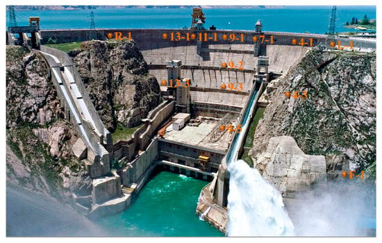
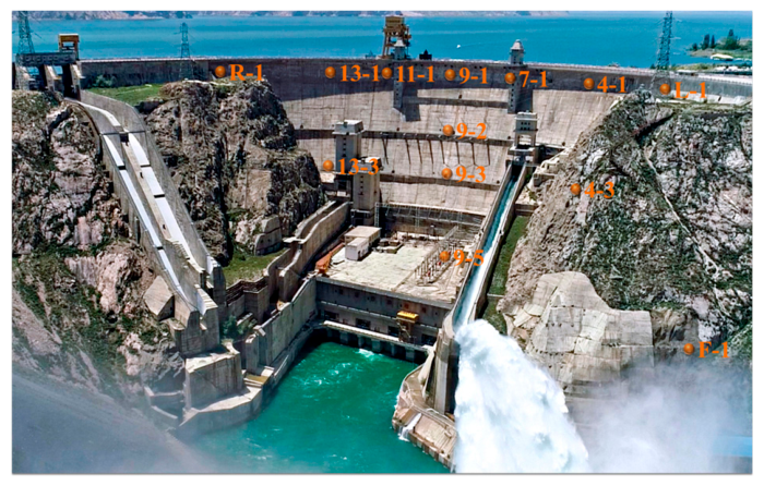
Because the project is situated in a high-seismicity region, a dynamic monitoring system was installed to evaluate the seismic performance of the dam. The system was initially established in 1983 and upgraded in 2009, which improved its dynamic range, sensitivity, impact resistance, and real-time monitoring capability. It comprises 13 measurement points. Twelve in-dam stations (L-1, 4-1, 4-3, 7-1, 9-1, 9-2, 9-3, 9-5, 11-1, 13-1, 13-3, and R-1) are distributed across four dam galleries at elevations of 2600, 2560, 2530, and 2463 m. One free-field reference station (F-1) is installed in the traffic tunnel of the powerhouse at elevation 2510 m. The view of the dam from the downstream and the locations of measurement points are shown in Figure 4. Each measurement point is equipped with a triaxial MEMS force-balanced accelerometer (TDA-23) oriented along the radial, tangential, and vertical directions. The sensors have a sensitivity of 2.5 V/g, a measurement range of ±2 g, and a dynamic range exceeding 100 dB. Ten in-dam accelerometers, providing 30 channels, are dedicated to operational modal analysis. Signals are sampled at 200 Hz and transmitted through 12-core waterproof shielded cables (RVVP) protected by PVC tubes. In each gallery, the cables are gathered and connected to a cable bridge in the gallery at the 2463 m level through an elevator shaft in dam block 11. They are then linked to TDE-324FA/CA digital data acquisition units in an equipment protection room in the auxiliary powerhouse. These units contain a GPS timing service for synchronization and a Wi-Fi router for data transmission. Acceleration time histories are continuously recorded at all measurement points for 60 min at a sampling frequency of 200 Hz. The collected data are preprocessed in real time by data servers and then stored in data concentrators for further analysis.

Figure 4. Downstream view of the dam and locations of the measurement points.

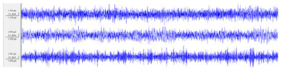
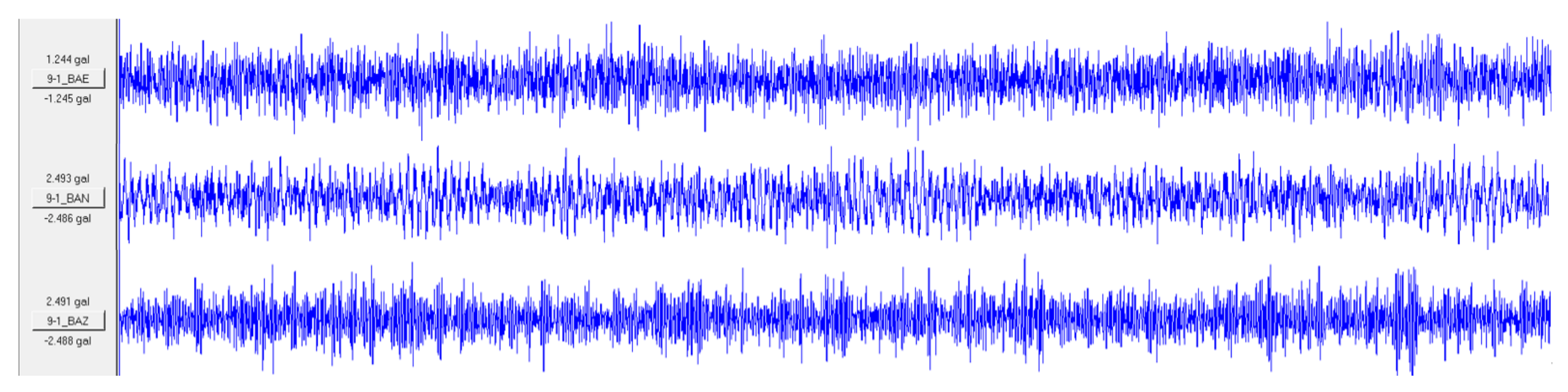
In this study, the ten in-dam triaxial force-balanced accelerometers, providing 30 channels, were used to characterize the dynamic properties of the dam. The acceleration time series used for modal identification were recorded under ambient excitation with a duration of 1 h and a sampling frequency of 200 Hz. As a representative example, the first 30 s of the acceleration time history recorded at measurement point 9-1, located at the center of the dam crest, is shown in Figure 5. The records indicate that the ambient vibration responses remain approximately stationary throughout the recording period. This stationarity satisfies the basic assumption of operational modal analysis and provides a reliable basis for the subsequent modal identification.

Figure 5. Ambient vibration acceleration time histories recorded at the measurement point 9-1.

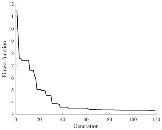
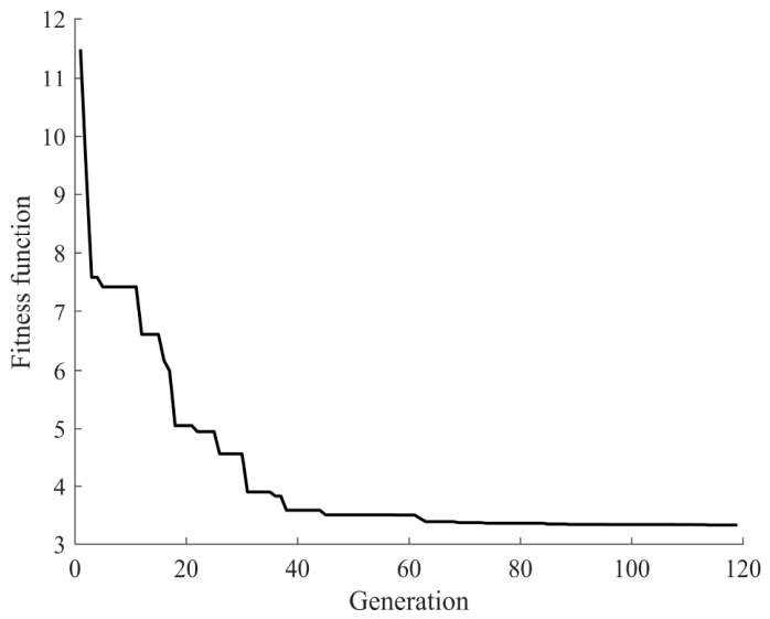
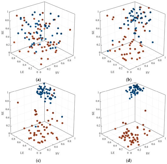
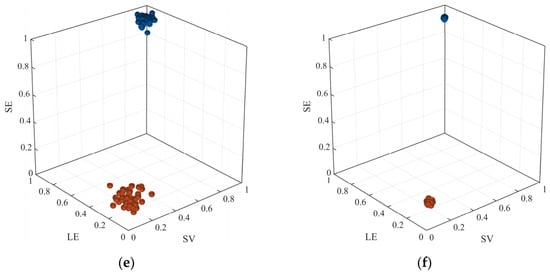
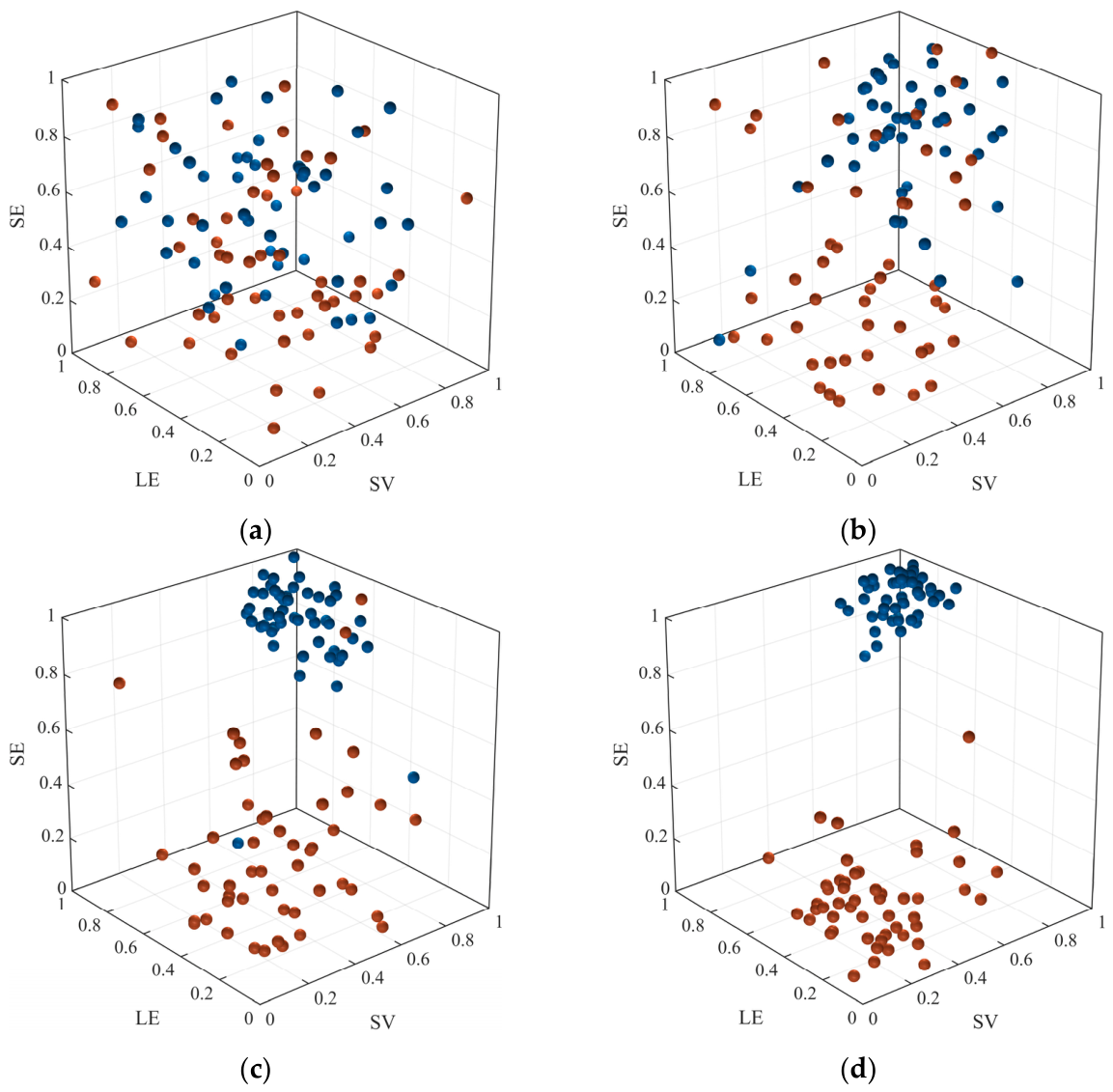
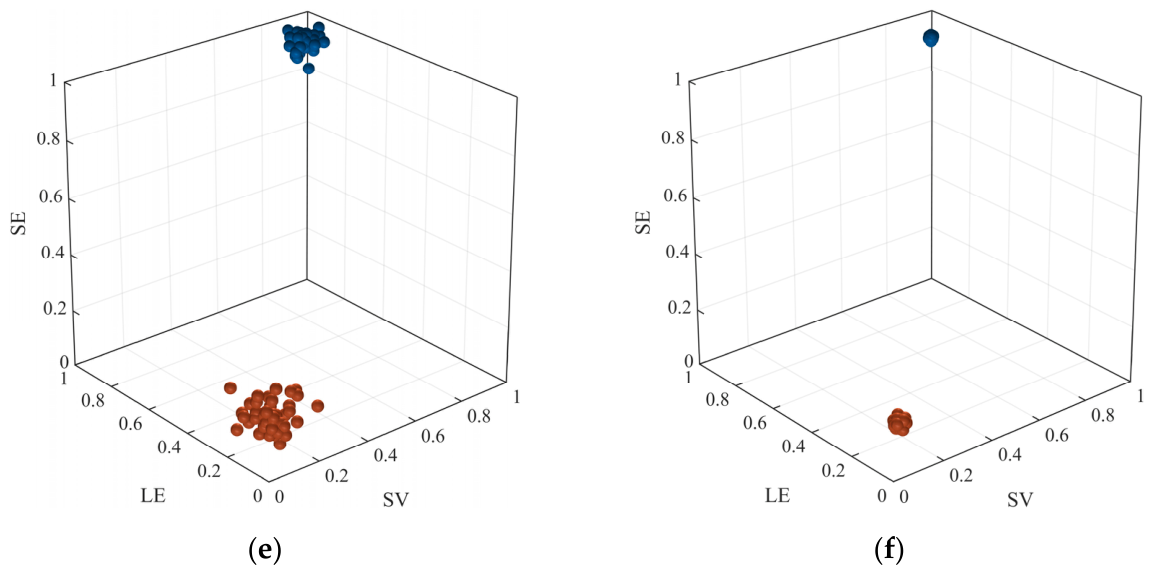
After detrending and decimating the acceleration time series to a sampling rate of 25 Hz, modal identification was conducted using the proposed method. The analytic modal responses were first separated, with the number of time lags p set to 100. The modal feature indices, namely spectral variance, length of envelope, and spectral entropy, were then computed for the 30 sets of separated analytic modal responses. Subsequently, the proposed blind feature clustering method was employed to automatically discriminate physical modes from spurious modes. In the algorithm, the population size N_p was set to 50, and the maximum number of generations g_max was set to 300. The termination condition was defined as either reaching the maximum number of generations or the sum of the differences in the best fitness values between adjacent generations over 30 consecutive iterations being less than a threshold of 0.001. The variation ranges of parameters F and CR were set as F_max = 0.9, F_min = 0.4, CR_max = 0.9, CR_min = 0.3. After 119 generations, the algorithm terminated automatically. The variation in the best fitness function of the population with the number of generations is shown in Figure 6. As can be seen, the algorithm converges rapidly, with the best fitness value stabilizing after a relatively small number of generations. This indicates that the algorithm has a strong global exploration capability in the early stage and gradually transitions to local exploitation for refined search in the later stage. The population distributions at several representative generations are shown in Figure 7. It can be observed that the population distribution becomes increasingly concentrated around two cluster centroids as the generations proceed, with modal feature index values approaching 0 and 1. These two centroids correspond to the clusters of physical modes and spurious modes, respectively, demonstrating that the proposed method can automatically discriminate between them.

Figure 6. Variation in the optimal fitness value of the population across generations.

Figure 7. Population distributions in the feature space at different representative generations. (a) Generation 1; (b) Generation 10; (c) Generation 20; (d) Generation 40; (e) Generation 80; (f) Generation 119.

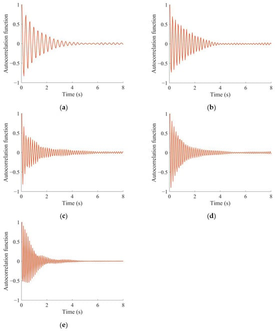
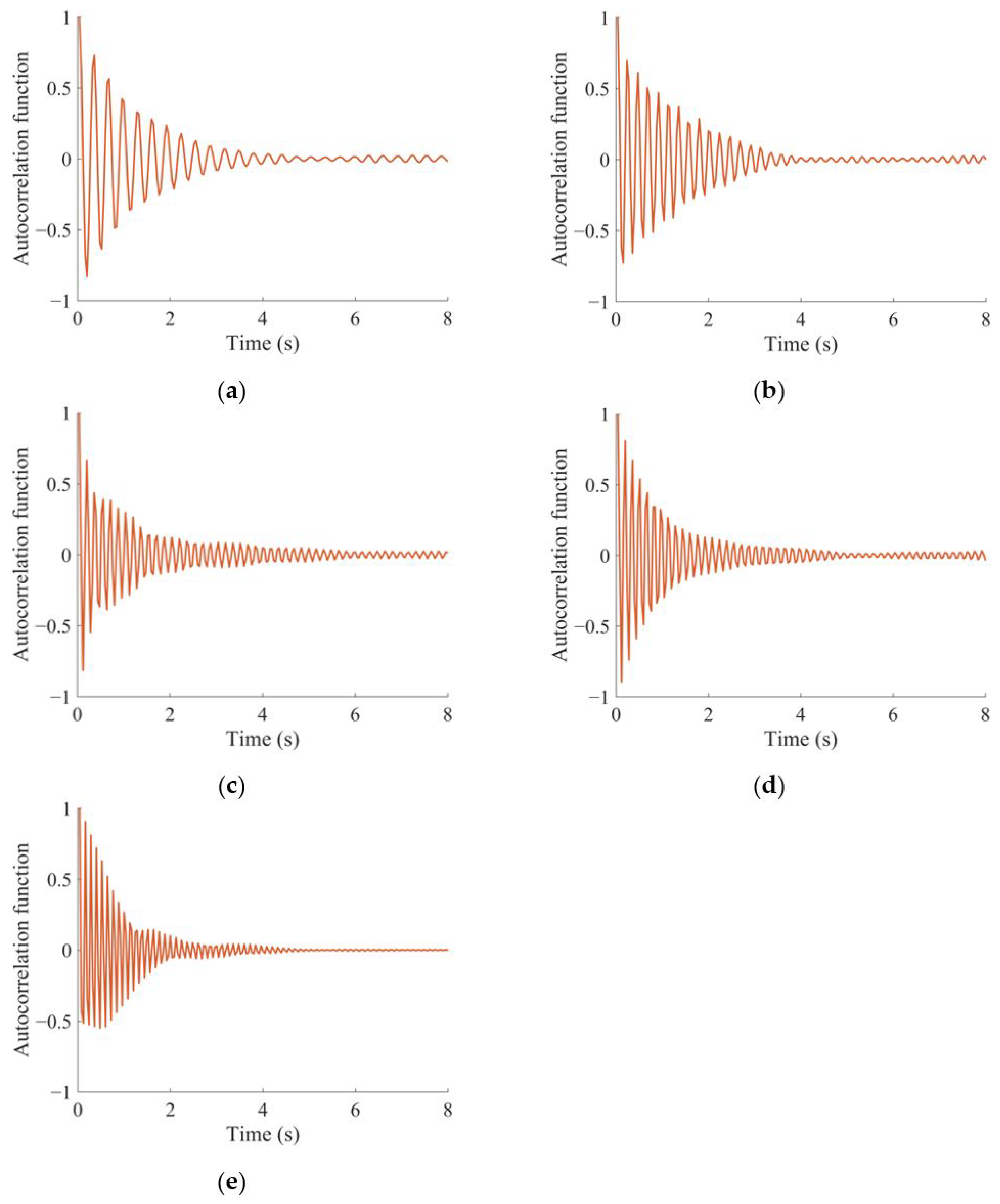
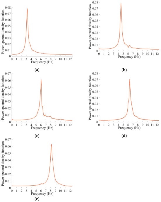
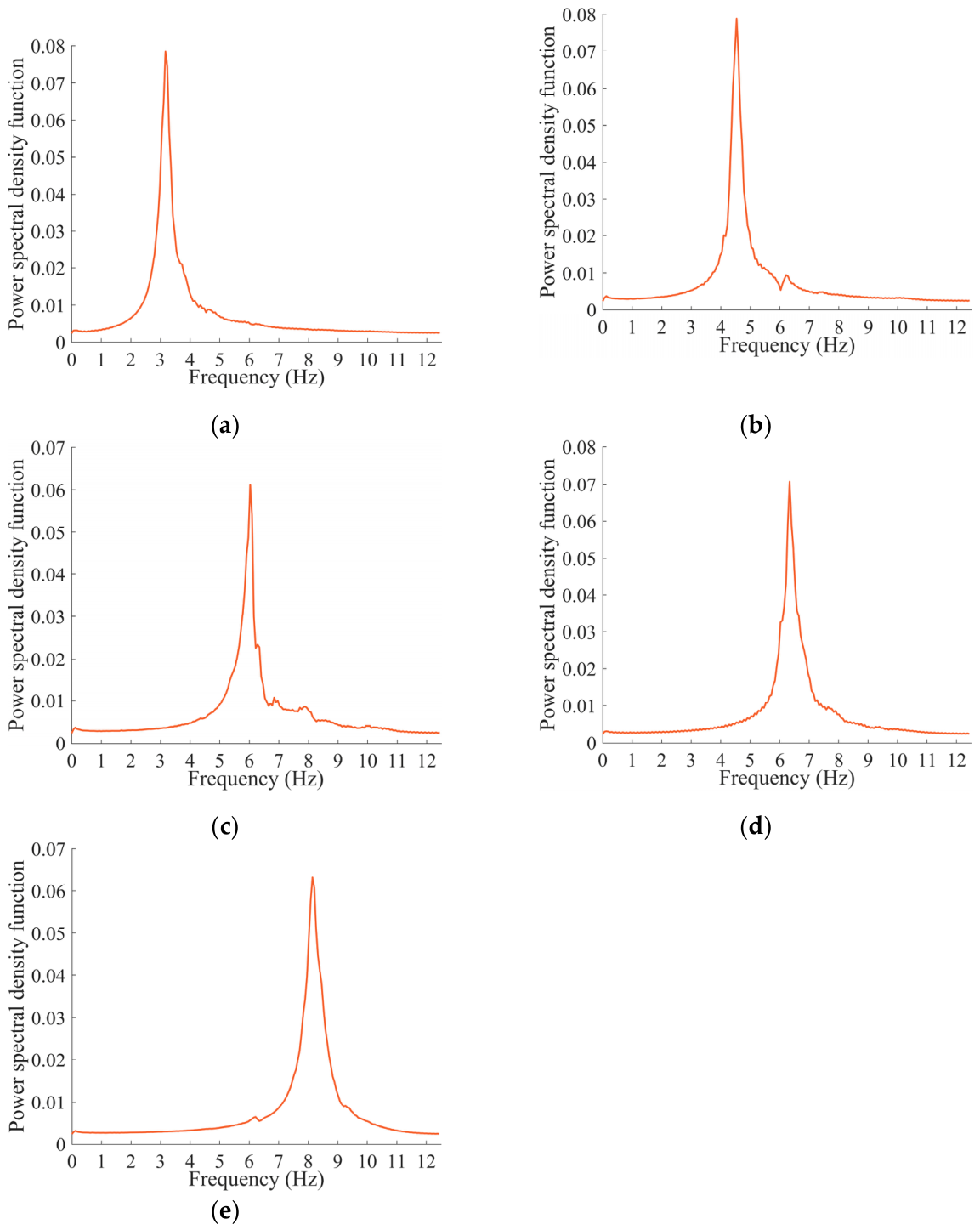
The physical-mode cluster contains five elements. The autocorrelation functions and auto-power spectral density functions of the modal responses for the five identified modes are presented in Figure 8 and Figure 9, respectively. As can be seen, the autocorrelation functions corresponding to the five physical modes exhibit exponentially decaying harmonic characteristics, while the auto-power spectral density functions show concentrated and clear single peaks near the natural frequencies, demonstrating satisfactory modal separation.

Figure 8. Autocorrelation functions of the modal responses corresponding to the five identified physical modes. (a–e) Modes 1–5.

Figure 9. Auto-power spectral density functions of the modal responses corresponding to the five identified physical modes. (a–e) Modes 1–5.

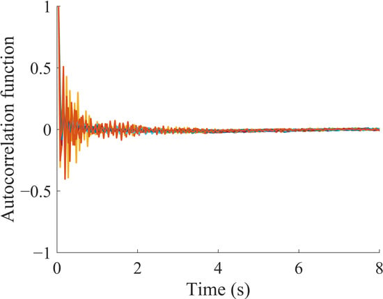
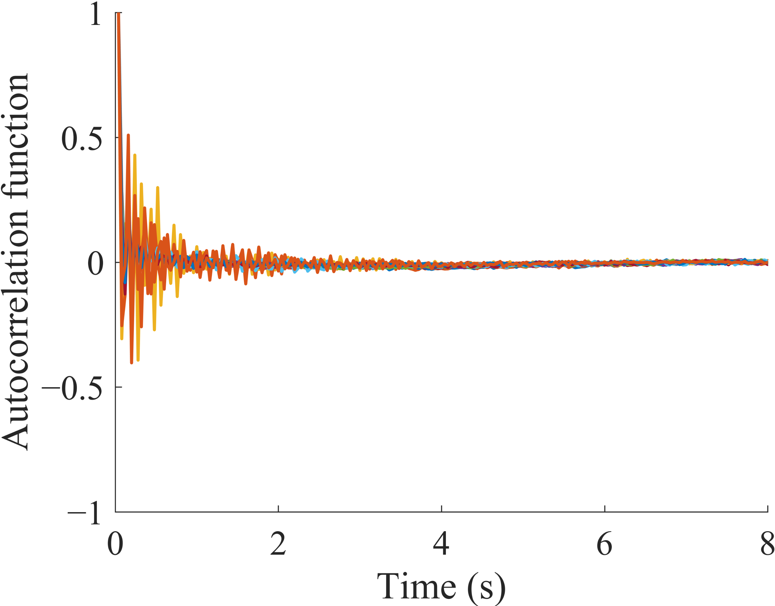
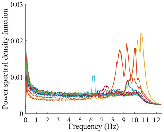
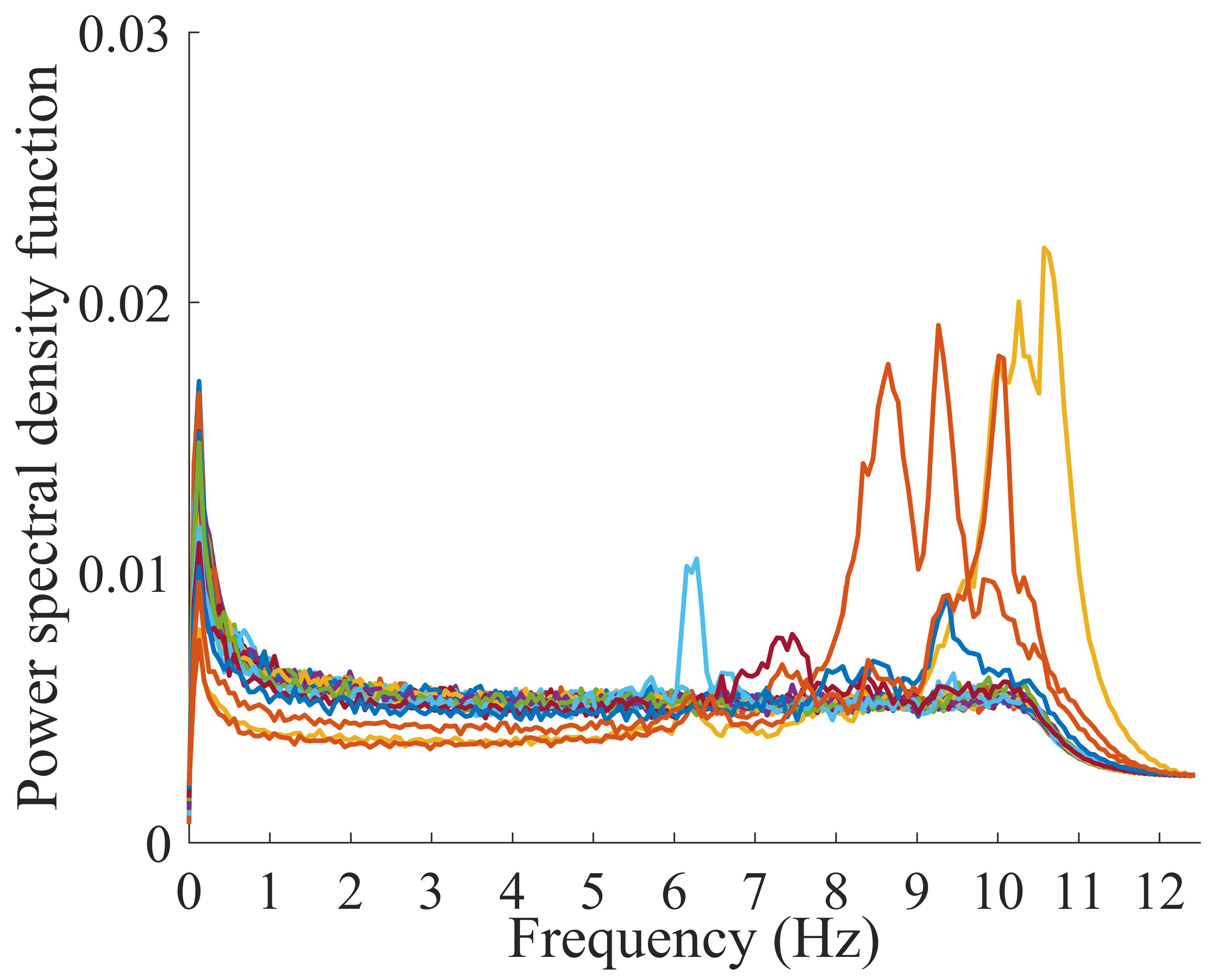
For comparison, the autocorrelation functions and auto-power spectral density functions of the modal responses of the spurious modes are presented in Figure 10 and Figure 11, respectively. The autocorrelation functions decay rapidly and irregularly, without consistent exponential behavior. In the frequency domain, the auto-power spectral density functions are characterized by dispersed spectral energy and multiple low-amplitude peaks. These features are clearly distinct from the concentrated single-peak spectra of the physical modes, further demonstrating that the proposed method can effectively reject spurious modes.

Figure 10. Autocorrelation functions of the modal responses corresponding to the spurious modes.

Figure 11. Auto-power spectral density functions of the modal responses corresponding to the spurious modes.

To examine the stability of the clustering, both the proposed method and conventional K-means clustering were run 100 times. For conventional K-means clustering, only 84 of the 100 runs produced the correct clustering result. 7 runs yielded empty clusters and thus failed to identify any structural-mode cluster. The remaining 9 runs erroneously assigned three spurious modes to the structural-mode cluster. In contrast, all 100 runs of the proposed DE-based clustering produced identical and correct clustering solutions. In contrast, all 100 runs of the proposed DE-based clustering produced identical and correct clustering solutions. These results effectively demonstrate that the proposed method overcomes the sensitivity of K-means to initial cluster centers and its tendency to fall into local optima, thereby yielding more stable and reliable clustering results.

As described, using the modal responses corresponding to the physical modes, the time-lagged output covariance matrices at different time lags were estimated and then assembled into a block Toeplitz matrix, with the number of block rows i set to 50. The block Toeplitz matrix was then decomposed by singular value decomposition, and the submatrix corresponding to the first 10 nonzero singular values was extracted to obtain the system matrix. The natural frequencies and damping ratios were estimated by eigenvalue decomposition. The identified natural frequencies of the first five modes are 3.27 Hz, 4.53 Hz, 6.04 Hz, 6.36 Hz, and 8.16 Hz, and the corresponding damping ratios are 3.3%, 2.5%, 1.4%, 1.5%, and 2.0%, respectively. The damping ratio of the first mode is higher than the values typically observed in lightweight structures. However, this value is not unusual for a large dam. The first structural mode is strongly affected by reservoir water added mass and radiation damping, foundation radiation damping, material damping, and joint- or crack-related energy dissipation, among other factors. These mechanisms collectively contribute to additional energy dissipation and thus to a relatively high first-mode damping ratio.

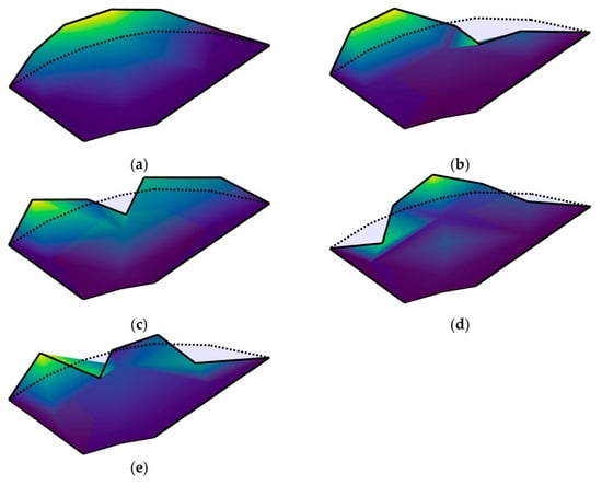
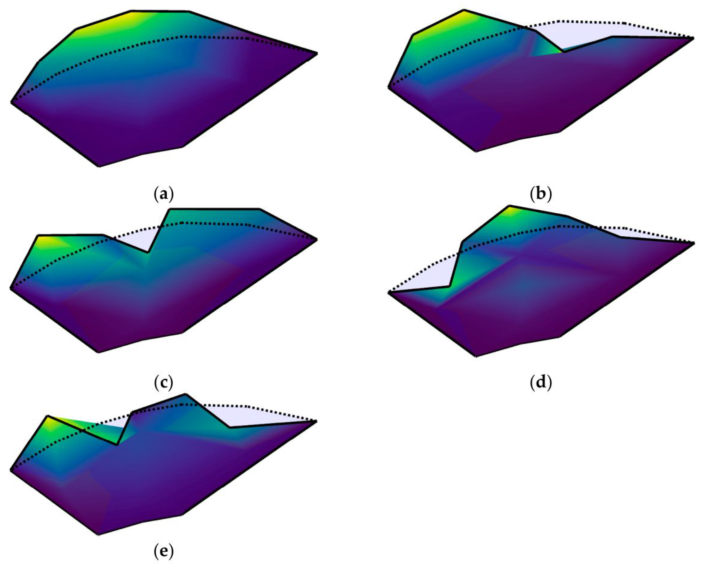
The structural mode shapes were obtained from the modal matrix corresponding to the five physical modes and are displayed in Figure 12. The symmetry characteristics of these five mode shapes are symmetric, antisymmetric, symmetric, symmetric, and antisymmetric, respectively. Such a symmetric–antisymmetric distribution is physically reasonable for a concrete arch-gravity dam and further confirms the reliability of the identified modal parameters.

Figure 12. Identified mode shapes of the five physical modes. (a–e) Modes 1–5.

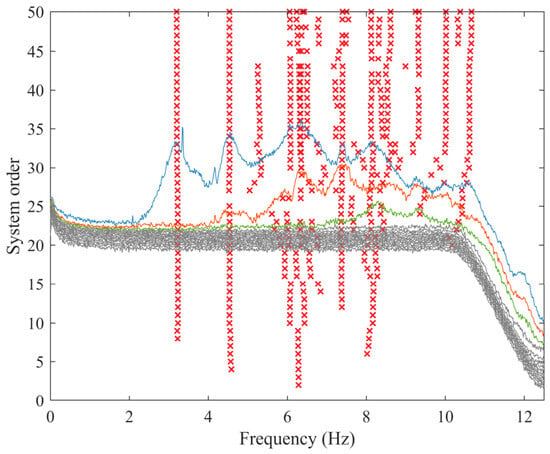
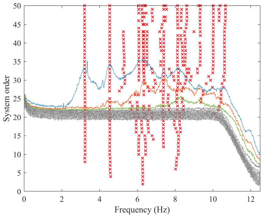
To demonstrate the advantages of the proposed method, Figure 13 presents the stabilization diagram obtained from SSI-COV, with the singular value spectra from FDD also shown for reference. In this figure, red crosses denote stable poles identified by SSI-COV, while colored lines represent singular value spectra estimated by FDD. It can be seen that the poles of the first two modes form stable alignments and are therefore relatively easy to distinguish. In contrast, the remaining three modes are intermixed with spurious poles, resulting in a scattered and disordered distribution, particularly for the closely spaced third and fourth modes. Consequently, effective separation becomes difficult, and automated discrimination between physical and spurious modes remains challenging, typically requiring subjective threshold selection and manual pole picking. In comparison, the proposed method effectively separates the modal responses of different modes, and feature clustering allows physical modes to be reliably distinguished from spurious ones. These results confirm the superiority of the proposed method.

Figure 13. Stabilization diagram obtained from SSI-COV.

The modal parameters identified by the proposed framework are compared with those obtained by the parametric SSI-COV method and the non-parametric FDD method, as summarized in Table 1. The natural frequencies identified by the proposed method are found to be closer to those obtained by the SSI-COV than to those obtained by the FDD. This indicates that the proposed framework retains the high accuracy of parametric OMA methods such as SSI, while avoiding the construction and interpretation of stabilization diagrams and thus the subjective, threshold-dependent pole selection that automated SSI-based approaches generally require. Table 1 also presents the finite element analysis results for the dam obtained by the China Institute of Water Resources and Hydropower Research (IWHR) [50]. Although the dam conditions considered in the calculations are different, the results remain consistent, which further validates the correctness of the modal parameter identification results obtained in this paper.

Table 1. Modal parameters obtained by the proposed method, SSI-COV, FDD and FEM.

Mode No.	Proposed Method		SSI-COV		FDD	FEM [50]	Description
	Freq. (Hz)	Damp. (%)	Freq. (Hz)	Damp. (%)	Freq. (Hz)	Freq. (Hz)
1	3.27	3.74	3.27	3.85	3.19	3.18	1st symmetric
2	4.53	2.90	4.53	2.60	4.56	4.61	1st antisymmetric
3	6.04	1.68	6.06	1.80	6.05	6.04	2nd symmetric
4	6.36	2.36	6.34	2.60	6.25	6.81	3rd symmetric
5	8.16	2.02	8.16	2.17	8.11	8.54	2nd antisymmetric

4. Conclusions

This study proposed an intelligent blind feature clustering framework for automated modal identification of concrete dams under ambient excitation. The framework builds on a recently developed blind subspace identification method that separates modal responses without constructing stabilization diagrams. Three modal feature indices, including spectral variance, total envelope length, and spectral entropy were extracted from the separated modal responses. An improved differential evolution algorithm integrated with K-means clustering was then introduced to search for the optimal clustering scheme in the feature space.

The framework was applied to a large concrete arch-gravity dam instrumented with triaxial accelerometers. The improved differential evolution algorithm converged automatically after 119 generations, and the population gradually concentrated around two cluster centers with modal feature index values close to 0 and 1, respectively. The physical-mode cluster contained five elements, while the remaining modes were assigned to the spurious cluster.

The physical modal responses exhibited exponentially decaying harmonic autocorrelation functions and concentrated single peaks in their auto-power spectral density functions. In contrast, the spurious modes showed irregular correlation decay and dispersed spectral energy. Based on the separated physical modal responses, natural frequencies, damping ratios, and mode shapes were estimated, and the identified mode shapes exhibited physically reasonable symmetric or antisymmetric patterns. For independent validation, the modal parameters identified by the proposed framework were compared with those obtained by SSI-COV, FDD, and FEM. The identified modal parameters agree well with these independent results, thereby supporting the correctness of the proposed method.

To examine the stability of the clustering, both the proposed method and conventional K-means clustering were run 100 times. Conventional K-means produced empty clusters or incorrect partitions in a number of runs, whereas all 100 runs of the proposed DE-based clustering yielded identical and correct solutions. These results indicate that the proposed method reduces the sensitivity of K-means to initial cluster centers and its tendency to fall into local optima, thereby providing more stable and reliable clustering results.

Compared with conventional approaches, the proposed framework avoids subjective threshold selection and manual pole picking, thereby reducing reliance on expert judgment and facilitating automated modal discrimination. These results suggest a promising approach for automated modal identification and long-term modal monitoring of concrete dams. Further validation using additional structures and monitoring periods is warranted before the framework is applied to safety assessment.

References

- Jia, J. A technical review of hydro-project development in China. Engineering 2016, 2, 302–312. [Google Scholar] [CrossRef] [Scilit]
- Kalkan Okur, E.; Okur, F.Y.; Günaydın, M.; Genç, A.F.; Altunışık, A.C. Long-term structural health monitoring of arch dams under environmental effects: Bayesian neural network-based frequency estimation. Measurement 2026, 292, 123318. [Google Scholar] [CrossRef] [Scilit]
- Wang, J.; Tong, F.; Gao, Z.; Cheng, L.; Zhao, S. Research on arch dam deformation safety early warning method based on effect separation of regional environmental variables and knowledge-driven approach. Water 2025, 17, 3217. [Google Scholar] [CrossRef] [Scilit]
- Wang, J.; Jin, F.; Zhang, C. Seismic safety of arch dams with aging effects. Sci. China Technol. Sci. 2011, 54, 522–530. [Google Scholar] [CrossRef] [Scilit]
- Prakash, G.; Dugalam, R.; Barbosh, M.; Sadhu, A. Recent advancement of concrete dam health monitoring technology: A systematic literature review. Structures 2022, 44, 766–784. [Google Scholar] [CrossRef] [Scilit]
- Bukenya, P.; Moyo, P.; Beushausen, H.; Oosthuizen, C. Health monitoring of concrete dams: A literature review. J. Civ. Struct. Health Monit. 2014, 4, 235–244. [Google Scholar] [CrossRef] [Scilit]
- Liu, X.; Li, Z.; Sun, L.; Khailah, E.Y.; Wang, J.; Lu, W. A critical review of statistical model of dam monitoring data. J. Build. Eng. 2023, 80, 108106. [Google Scholar] [CrossRef] [Scilit]
- Gu, C.; Wu, B.; Chen, Y. High-robust displacement prediction model for super-high arch dams integrating wavelet de-noising and improved random forest. Water 2023, 15, 1271. [Google Scholar] [CrossRef] [Scilit]
- Cao, E.; Bao, T.; Yuan, R.; Hu, S. Hierarchical prediction of dam deformation based on hybrid temporal network and load-oriented residual correction. Eng. Struct. 2024, 308, 117949. [Google Scholar] [CrossRef] [Scilit]
- Liu, Y.; Zheng, D.; Georgakis, C.; Kabel, T.; Cao, E.; Wu, X.; Ma, J. Deformation analysis of an ultra-high arch dam under different water level conditions based on optimized dynamic panel clustering. Appl. Sci. 2022, 12, 481. [Google Scholar] [CrossRef] [Scilit]
- Gu, C.; Wang, Y.; Gu, H.; Hu, Y.; Yang, M.; Cao, W.; Fang, Z. A combined safety monitoring model for high concrete dams. Appl. Sci. 2022, 12, 12103. [Google Scholar] [CrossRef] [Scilit]
- Bao, T.; Li, J.; Lu, Y.; Gu, C. IDE-MLSSVR-based back analysis method for multiple mechanical parameters of concrete dams. J. Struct. Eng. 2020, 146, 04020155. [Google Scholar] [CrossRef] [Scilit]
- Li, H.; Lou, J.; Li, F.; Yang, G.; Ouyang, Y. A Deep Learning Framework for Deformation Monitoring of Hydraulic Structures with Long-Sequence Hydrostatic and Thermal Time Series. Water 2025, 17, 1814. [Google Scholar] [CrossRef] [Scilit]
- Cheng, L.; Tian, K.; Yuan, X.; Wang, Z.; Ma, C.; Li, B.; Tong, F.; Xu, Z. Research on the influence of environmental variables on the natural frequency of concrete gravity dams via mechanism analysis and data-driven models. Mech. Syst. Signal Process. 2025, 239, 113311. [Google Scholar] [CrossRef] [Scilit]
- Liu, B.; Li, H.; Liu, F.; Huang, W.; Wang, G.; Wang, H.; Wang, W.; Tang, Y.; Liu, H. Beat vibration analysis model of overflow dam pier under discharge excitation based on adaptive VMD and automatic operational modal analysis. Mech. Syst. Signal Process. 2024, 211, 111201. [Google Scholar] [CrossRef] [Scilit]
- Li, J.; Gao, J.; Zhang, S.; Mircevska, V.; Cao, M. Output-only modal identification of civil engineering structures based on parametric complexity pursuit. Sensors 2026, 26, 2417. [Google Scholar] [CrossRef] [Scilit] [PubMed]
- Mostafaei, H.; Ghamami, M.; Aghabozorgi, P. Modal identification of concrete arch dam by fully automated operational modal identification. Structures 2021, 32, 228–236. [Google Scholar] [CrossRef] [Scilit]
- Li, H.; Liao, W.; Liu, B.; Huang, W.; Tang, Y.; Zhu, H. Identification of operational modal parameters for a large floodgate under hydraulic excitation using the blind source separation improved by Hankel matrix singular value and adaptive variational mode decomposition. J. Civ. Struct. Health Monit. 2025, 15, 1689–1708. [Google Scholar] [CrossRef] [Scilit]
- Pereira, S.; Magalhães, F.; Gomes, J.P.; Cunha, Á.; Lemos, J.V. Vibration-based damage detection of a concrete arch dam. Eng. Struct. 2021, 235, 112032. [Google Scholar] [CrossRef] [Scilit]
- Qiu, J.; He, W.; Long, C.; Zhang, Y.; Liu, X.; Xu, P.; Sun, L.; Zhang, C.; Cheng, L.; Lu, W. Dynamic Response-Based Safety Monitoring and Damage Identification of Concrete Arch Dams via PSO-LSTM. Sensors 2026, 26, 1136. [Google Scholar] [CrossRef] [Scilit] [PubMed]
- Xiang, Z.; Pan, J.; Wang, J.; Dong, C. Improved approach for vibration-based structural health monitoring of arch dams during seismic events and normal operation. Struct. Control Health Monit. 2022, 29, 2955. [Google Scholar] [CrossRef] [Scilit]
- Brinker, R.; Ventura, C.E. Introduction to Operational Modal Analysis; John Wiley & Sons, Ltd.: Chichester, UK, 2015. [Google Scholar]
- Reynders, E. System identification methods for (operational) modal analysis: Review and comparison. Arch. Comput. Methods Eng. 2012, 19, 51–124. [Google Scholar] [CrossRef] [Scilit]
- Liu, W.; Liu, B.; Feng, H.; Wang, B.; Yang, N.; Gao, Y. Field dynamic testing and adaptive dynamic characteristic identification of steel tower structures in high-speed railway stations under limited sensor configurations. Buildings 2025, 15, 3754. [Google Scholar] [CrossRef] [Scilit]
- Liu, X.; Liu, S.; Su, Y.; Wang, J.; Xie, S.; Luo, Y.; Zhang, Y. An extended modal approach for modal parameter identification of structure under the existence of harmonic excitations. Mech. Syst. Signal Process. 2024, 213, 111334. [Google Scholar] [CrossRef] [Scilit]
- Mostafaei, H.; Ghamami, M. State of the art in automated operational modal identification: Algorithms, applications, and future perspectives. Machines 2025, 13, 39. [Google Scholar] [CrossRef] [Scilit]
- Mostafaei, H. Modal identification techniques for concrete dams: A comprehensive review and application. Sci 2024, 6, 40. [Google Scholar] [CrossRef] [Scilit]
- Alegre, A.; Oliveira, S.; Proença, J.; Mendes, P.; Carvalho, E. A finite element formulation for true coupled modal analysis and nonlinear seismic modeling of dam-reservoir-foundation systems: Application to an arch dam and validation. Infrastructures 2025, 10, 193. [Google Scholar] [CrossRef] [Scilit]
- Cheng, L.; Tian, K.; Yuan, X.; Li, Z.; Tong, F.; Ma, C.; Li, B. Non-parametric modal identification and monitoring of concrete dams under ambient excitations. Appl. Math. Model. 2025, 148, 116271. [Google Scholar] [CrossRef] [Scilit]
- Brincker, R.; Andersen, P.; Jacobsen, N.J. Automated frequency domain decomposition for operational modal analysis. In Proceedings of the 25th International Modal Analysis Conference, Orlando, FL, USA, 19–22 February 2007. [Google Scholar]
- Magalhães, F.; Cunha, Á.; Caetano, E. Dynamic monitoring of a long span arch bridge. Eng. Struct. 2008, 30, 3034–3044. [Google Scholar] [CrossRef] [Scilit]
- Rainieri, C.; Fabbrocino, G. Automated output-only dynamic identification of civil engineering structures. Mech. Syst. Signal Process. 2010, 24, 678–695. [Google Scholar] [CrossRef] [Scilit]
- Peeters, B.; De Roeck, G. One-year monitoring of the Z24-Bridge: Environmental effects versus damage events. Earthq. Eng. Struct. Dyn. 2001, 30, 149–171. [Google Scholar] [CrossRef] [Scilit]
- Magalhães, F.; Cunha, Á.; Caetano, E. Online automatic identification of the modal parameters of a long span arch bridge. Mech. Syst. Signal Process. 2009, 23, 316–329. [Google Scholar] [CrossRef] [Scilit]
- Reynders, E.; Houbrechts, J.; De Roeck, G. Fully automated (operational) modal analysis. Mech. Syst. Signal Process. 2012, 29, 228–250. [Google Scholar] [CrossRef] [Scilit]
- Ubertini, F.; Gentile, C.; Materazzi, A.L. Automated modal identification in operational conditions and its application to bridges. Eng. Struct. 2013, 46, 264–278. [Google Scholar] [CrossRef] [Scilit]
- Cabboi, A.; Magalhães, F.; Gentile, C.; Cunha, Á. Automated modal identification and tracking: Application to an iron arch bridge. Struct. Control Health Monit. 2017, 24, e1854. [Google Scholar] [CrossRef] [Scilit]
- Li, S.; Pan, J.; Luo, G.; Wang, J. Automatic modal parameter identification of high arch dams: Feasibility verification. Earthq. Eng. Eng. Vib. 2020, 19, 953–965. [Google Scholar] [CrossRef] [Scilit]
- Li, B.; Liang, W.; Yang, S.; Zhang, L. Automatic identification of modal parameters for high arch dams based on SSI, SSA and K-means algorithm. Appl. Soft Comput. 2023, 138, 110201. [Google Scholar] [CrossRef] [Scilit]
- Wu, Y.; Kang, F.; Wan, G.; Li, H. Automatic operational modal analysis for concrete arch dams integrating improved stabilization diagram with hybrid clustering algorithm. Mech. Syst. Signal Process. 2025, 224, 112011. [Google Scholar] [CrossRef] [Scilit]
- Li, H.; Zeng, S.; Liu, B.; Wang, G.; Tang, Y.; Wang, W.; Huang, W. Automatic operational modal analysis for high arch dams using enhanced SSI-COV with adaptive MVMD and improved FCM clustering algorithm. Adv. Eng. Inform. 2026, 71, 104257. [Google Scholar] [CrossRef] [Scilit]
- Li, J.; Bao, T.; Ventura, C.E. An automated operational modal analysis algorithm and its application to concrete dams. Mech. Syst. Signal Process. 2022, 168, 108707. [Google Scholar] [CrossRef] [Scilit]
- Li, J.; Bao, T.; Ventura, C.E. A robust methodology for output-only modal identification of civil engineering structures. Eng. Struct. 2022, 270, 114764. [Google Scholar] [CrossRef] [Scilit]
- Li, J.; Cao, M.; Bao, T.; Li, T. A robust operational modal analysis method and its application to a concrete arch-gravity dam. In Proceedings of the 10th International Operational Modal Analysis Conference, Naples, Italy, 21–24 May 2024. [Google Scholar]
- McNeill, S. An analytic formulation for blind modal identification. J. Vib. Control 2011, 18, 2111–2121. [Google Scholar] [CrossRef] [Scilit]
- McNeill, S.; Zimmerman, D. A framework for blind modal identification using joint approximate diagonalization. Mech. Syst. Signal Process. 2008, 21, 2335–2358. [Google Scholar] [CrossRef] [Scilit]
- Belouchrani, A.; Abed-Meraim, K.; Cardoso, J.-F.; Moulines, E. A blind source separation technique using second-order statistics. IEEE Trans. Signal Process. 1997, 45, 434–444. [Google Scholar] [CrossRef] [Scilit]
- Rainieri, C.; Fabbrocino, G. Development and validation of an automated operational modal analysis algorithm for vibration-based monitoring and tensile load estimation. Mech. Syst. Signal Process. 2015, 60–61, 512–534. [Google Scholar] [CrossRef] [Scilit]
- Qin, A.K.; Huang, V.L.; Suganthan, P.N. Differential evolution algorithm with strategy adaptation for global numerical optimization. IEEE Trans. Evol. Comput. 2009, 13, 398–417. [Google Scholar] [CrossRef] [Scilit]
- Yang, J.; Hou, S. Solving the dynamic response of arch dams using orthogonal iteration. Water Power 1981, 6, 57–61+79. (In Chinese) [Google Scholar]
Disclaimer/Publisher’s Note: The statements, opinions and data contained in all publications are solely those of the individual author(s) and contributor(s) and not of MDPI and/or the editor(s). MDPI and/or the editor(s) disclaim responsibility for any injury to people or property resulting from any ideas, methods, instructions or products referred to in the content. |
© 2026 by the authors. Licensee MDPI, Basel, Switzerland. This article is an open access article distributed under the terms and conditions of the Creative Commons Attribution (CC BY) license.