A Reliability Audit of AI-Assisted Movement Assessment for Physical Education: A Reproducible Public-Data Stress Test of Movement Classifiers

Featured Application

Reliability auditing of AI-assisted movement classifiers as a precondition for teacher-reviewed assessment in higher physical education; the audit framework, including quality-aware deferral as a teacher-review trigger, is the intended practical output. Educational validity remains to be established in classroom studies.

Abstract

AI-assisted movement assessment is being considered for physical education, but such systems must remain dependable when observations degrade. This study provides a reliability audit of movement classification before any classroom adoption, treating trustworthy behavior under imperfect sensing as a precondition for AI-supported instruction. Six fixed predictors, including a predefined random forest, were evaluated on 2000 University of Idaho Physical Rehabilitation Movement Data (UI-PRMD) repetitions from ten healthy participants, with five participant-separated folds and controlled perturbations that preserve the source labels. The audit separates three failure layers that accuracy alone conflates: ranking quality, fixed-threshold decisions, and probability calibration. The forest reached 83.6% clean balanced accuracy; temperature scaling improved calibration; and a quality-aware deferral rule withheld unreliable predictions, a mechanism we interpret as a teacher-review trigger rather than an automated grading decision. Under only 2-degree independent angular noise, fixed-threshold decisions collapsed (52.8%) while ranking information largely survived (AUC 0.855), and severity-matched cutpoint adaptation recovered most decisions (77.0%). Classification was stable under 30% missing rotations and 10-Hz downsampling. Sensitivity analyses over the deferral-score coefficients, temperature stability across folds, and leave-one-subject-out influence confirmed these conclusions are not artifacts of particular parameter choices. The audit is fully reproducible and dataset-specific; educational effectiveness, classroom transfer, and physical-sensor robustness remain untested and are prerequisites for instructional deployment.

1. Introduction

Artificial intelligence (AI) research in physical education (PE) includes movement observation, instructional analysis, and individualized feedback [1,2,3]. Recent systematic reviews describe AI applications across teaching, learning, and assessment in PE and sports [3,4]. Movement classifiers can support an educator’s decisions, but their labels need a clear interpretation. Separating correct from non-optimal repetitions does not validate a measure of learning, effort, fitness, or achievement. Before any classroom use, the conditions under which such a classifier becomes unreliable must be known, because a teacher who receives silently degraded automated judgments cannot compensate for them. Reliability auditing is therefore a precondition for AI integration in education; it does not replace pedagogical evaluation.

In university PE, studies have used predictive models to examine student engagement and the relationship between digital technology and teaching quality [5,6]. Video analysis has also been applied to classroom teaching behavior [7]. Reviews of AI in PE and higher education discuss the educational context and educators’ roles [8,9]. These instructional outcomes differ from the execution quality of an individual repetition, and they typically assume that the underlying measurement is trustworthy. Here, the focus is on the reliability of movement assessment when the observations deteriorate, which is the layer that must hold before any of those instructional applications can be trusted. Classroom effects are outside the evaluation.

Public motion datasets allow reproducible testing without recruiting a new student cohort. Applications in table tennis and telerehabilitation use pose estimation to extract movement information [10,11]. OpenPose estimates two-dimensional keypoints [12]; model-based optimization and smartphone-based biomechanical analysis add other modeling steps toward kinematic measurements [13,14]. Capture conditions and validation targets vary across these systems, and recent surveys of action quality assessment and 3D pose estimation document how quickly this landscape is moving [15,16]. Exercise recognition, execution assessment, injury risk, and educational grading are separate tasks and require different evidence.

An unchanged movement may be recorded with noisy rotations, missing joints, or fewer temporal samples. Such observations may not support a reliable classification. Probability calibration aligns predicted probabilities with observed frequencies. Selective prediction allows the system to withhold some classifications from automated reporting. Both retain the original label definition. Evaluation must report the error among retained predictions, the fraction withheld, and the behavior of a selection rule outside its calibration distribution.

We evaluate a fixed pipeline on the Kinect recordings of the University of Idaho Physical Rehabilitation Movement Data (UI-PRMD) [17]. It uses circular summaries of local Euler rotations and lightweight classifiers, followed by held-out temperature scaling and a quality-aware deferral score. Each of five folds separates training, calibration, and test participants. Controlled perturbations preserve the original labels, so classification, probability quality, and reporting behavior can be compared on the same repetitions.

Aim

The aim of this study is to quantify, on a public dataset with participant-separated evaluation, how far a fixed movement-classification pipeline can be trusted when its kinematic observations degrade, and which parts of the failure are properties of the decision rule rather than the learned representation.

The evaluation asks how well fixed classifiers separate the source labels for unseen people, whether calibration and quality-aware selection improve probability quality or retained error, and how these results change under degraded observations. The contributions of the study are:

1.

A reproducible, participant-separated stress test of a fixed movement-classification pipeline on public UI-PRMD Kinect data, with all predictions, code, and seeds released;

2.

An evaluation design that separates ranking quality, fixed-threshold decisions, and probability calibration, showing that these layers fail at different perturbation severities;

3.

A quality-aware deferral rule whose withholding behavior is interpreted as a teacher-review trigger, connecting the audit to teacher-in-the-loop use of AI in education;

4.

Sensitivity analyses (deferral-coefficient grid, cross-fold temperature stability, leave-one-subject-out influence, and small-sample t intervals) that test whether the conclusions depend on particular parameter choices.

The study examines classification failure and excessive deferral without proposing a new classifier architecture or testing a teaching intervention.

2. Related Work

2.1. Movement Recognition and Assessment: A Structured Overview

Recent work on movement recognition and assessment can be organized along four axes: sensing modality, motion representation, supervision signal, and validation protocol. Table 1 summarizes representative studies on the two public datasets most relevant here.

2.1.1. Sensing Modality

Studies use RGB video, depth, inertial units, and marker-based or markerless optical capture. RGB-camera frameworks with spatiotemporal transformers reach assessment-grade performance on UI-PRMD and KIMORE [18]. Graph convolutional networks over skeleton sequences are the dominant skeleton-based approach [19,20,21], and expert-knowledge-based graph convolutions inject anatomical priors into the architecture [22]. Reviews of 3D human pose estimation cover the accuracy limits of markerless pipelines [16].

2.1.2. Motion Representation

Representations range from raw joint-angle sequences to learned spatiotemporal embeddings. View-invariant assessment and rehabilitation models based on graph convolution or spatiotemporal sequences address the representation problem [19,20,21]. Supervised contrastive learning with hard and soft negatives has produced the current strongest published results on UI-PRMD quality scoring [23]. Closer to the present study, interpretable feature-prioritized CNNs evaluate execution correctness on UI-PRMD and KIMORE [24], and a survey of video-surveillance action recognition covers the deep-learning toolbox for recognition from visual data [25].

2.1.3. Supervision Signal

Dataset annotations differ in what the label means: binary intended correctness (UI-PRMD), clinician questionnaire scores (KIMORE), or continuously derived quality scores [17,26,27]. The supervision signal determines what any reported accuracy measures, and binary correctness labels cannot validate continuous quality or grading claims.

2.1.4. Validation Protocol

Published results differ in participant separation, repetition splits, and reported metrics; random repetition splits inflate performance relative to participant-separated evaluation [28]. The studies in Table 1 use heterogeneous protocols, which is why we compare fixed conventional predictors within our own protocol rather than ranking architectures across papers.

Table 1. Representative recent studies on UI-PRMD and KIMORE. Protocols differ (sensor, target, split), so scores are not directly comparable; the table positions the present audit rather than benchmarking it.

Study	Task and Data	Protocol Note	Year
Liao et al. [27]	Continuous quality scores, reduced Vicon UI-PRMD	Random 70/30 + LOPO check	2020
He et al. [22]	Skeleton assessment, KIMORE	Expert-knowledge GCN	2024
Raihan et al. [24]	Correctness + quality, UI-PRMD and KIMORE	Interpretable SE-CNN	2025
Karlov et al. [23]	Quality scoring, UI-PRMD, IRDS, KIMORE	Contrastive learning	2025
Kourbane et al. [21]	Assessment, UI-PRMD	Sequential ST-GCN	2025
Chander et al. [18]	Assessment, KIMORE	RGB spatiotemporal transformer	2025
Present audit	Binary correctness stress test, Kinect UI-PRMD	Participant-separated folds + perturbations	2026

Table 1. Representative recent studies on UI-PRMD and KIMORE. Protocols differ (sensor, target, split), so scores are not directly comparable; the table positions the present audit rather than benchmarking it.

Study	Task and Data	Protocol Note	Year
Liao et al. [27]	Continuous quality scores, reduced Vicon UI-PRMD	Random 70/30 + LOPO check	2020
He et al. [22]	Skeleton assessment, KIMORE	Expert-knowledge GCN	2024
Raihan et al. [24]	Correctness + quality, UI-PRMD and KIMORE	Interpretable SE-CNN	2025
Karlov et al. [23]	Quality scoring, UI-PRMD, IRDS, KIMORE	Contrastive learning	2025
Kourbane et al. [21]	Assessment, UI-PRMD	Sequential ST-GCN	2025
Chander et al. [18]	Assessment, KIMORE	RGB spatiotemporal transformer	2025
Present audit	Binary correctness stress test, Kinect UI-PRMD	Participant-separated folds + perturbations	2026

Dataset annotations also differ, as noted above. KIMORE provides clinician questionnaire evaluations and physician-defined features for five low-back-pain rehabilitation exercises, with healthy and motor-impaired participants [26]. UI-PRMD contains correct and deliberately non-optimal performances by healthy volunteers [17]. Liao et al. subsequently derived continuous quality scores using movement-performance metrics and learned them with a deep spatiotemporal network [27]. Their UI-PRMD analysis used a manually reduced set, 117-dimensional Vicon angular sequences, exercise-specific score prediction, a random 70/30 repetition split, and an additional leave-one-subject-out check. These derived scores are not independent clinical or teacher ratings. Our full segmented Kinect rotation set, pooled binary task, and separate training/calibration/test participants therefore cannot support a direct comparison of published scores. We compare fixed conventional predictors within the present protocol rather than claim a state-of-the-art ranking.

Feedback studies in PE evaluate motor-skill learning [29], while work on objective assessment in children links measurement to a particular population and purpose [30]. Systematic reviews of AI in education emphasize teacher agency and human–AI collaboration as conditions for classroom adoption [3]. Classifier accuracy alone says little about whether feedback is understandable or useful. The present labels do not identify an anatomical cause or prescribe a correction, and we did not measure learner responses. An instructional system would also need evidence on teacher interpretation, feedback timing, fairness, and learning outcomes.

2.2. Measurement Reliability, Noise, and Validation

Comparative and repeated-session studies of markerless motion capture examine measurement validity and repeatability [31,32,33]. Reviews cover the limitations of single-camera healthcare applications and three-dimensional pose estimation [34,35]; camera viewing angle is one source of variation in validity [36]. Recent reliability studies of markerless pose estimation for joint range-of-motion measurement report acceptable validity for some joints and tasks but systematic error for others [37], and reliability-centred evaluation frameworks trace how pose-estimation error propagates into downstream motor biomarkers [38]. Skeleton-based action recognition itself degrades under joint noise, motivating dedicated noise-robust architectures [39]. These studies measure sensing error at its source; the present audit instead injects controlled error at the observation level and traces its effect through a complete classification pipeline. Synchronized video, motion-capture, and force-plate datasets permit direct measurement validation [40]. We use released Euler observations to perturb the same repetition under controlled conditions. This approach cannot reproduce the full sensing process.

Data partitioning must account for repeated movements from each participant [28]. A random repetition split can place the same person’s movement characteristics in both training and testing. We separate participants within each fold and resample participants for uncertainty summaries. The 2000 repetitions come from ten independent people; corruption seeds add perturbation realizations, not participants.

2.3. Calibration, Deferral, and Uncertainty

Random forests model nonlinear feature interactions without learning a large temporal representation [41]. Their discrimination and probability calibration need separate evaluation: predicted probabilities may disagree with observed frequencies even when decisions are useful [42]. Temperature scaling fits a single post-processing parameter [43], which limits fitting complexity when a fold has only two calibration participants. Calibration remains an active concern in applied deep learning, including medical imaging, where uncertainty-aware training improves probability quality [44]. Uncertainty about transfer to other participants or observation conditions remains.

Reject-option classification trades automated decisions against withheld cases; a recent survey systematizes this family of methods and their guarantees [45,46]. In an error-retention analysis, “risk” means classification error and has no injury interpretation. A reporting threshold must be fixed without test outcomes, even if a score ranks test predictions well. Conformal prediction provides another uncertainty framework under its assumptions [47]; we use neither a conformal procedure nor a coverage guarantee. The empirical evaluation reports calibration diagrams, matched-retention diagnostics, and independently calibrated threshold behavior separately.

3. Materials and Methods

3.1. Data Provenance and Audit

UI-PRMD contains ten rehabilitation-oriented exercises performed by ten healthy participants, recorded with a Microsoft Kinect depth sensor (Microsoft Corporation, Redmond, WA, USA) [17]. According to the source paper, the volunteers were graduate students or faculty, with a mean age of 29.3 years and standard deviation of 5.85 years. We use these published demographic descriptions. Recruitment was not for a university PE course, so transfer to a PE cohort remains to be evaluated.

The analyzed release consists of four archives: complete correct and non-optimal movements and segmented versions of both. All four archives were hashed using SHA-256. The analysis includes only Kinect angle files from the two segmented archives. Each included file was read with archive checksum verification; corresponding position files were checked for matching length, shape, and finite values. Other archive members were not exhaustively checksum-tested. The release yielded exactly 2000 valid Kinect repetitions, balanced between the two labels. Every subject contributes ten repetitions per exercise per class, giving 200 records per person. No selected Kinect repetition was excluded. Vicon records and unsegmented duplicates were excluded by protocol.

The included data contain 151,158 frames at a nominal sampling rate of 30 Hz. Repetition length ranges from 28 to 179 frames, with median 72 frames; nominal durations range from 0.90 to 5.93 s. The released angle files do not contain capture timestamps. The prediction unit is an entire segmented repetition. The independent evaluation unit is the subject. Table 2 summarizes the sample and fixed protocol. Source archives and individual file hashes, filenames, exercise identifiers, coded participant identifiers, and original labels are retained in the Supplementary Materials.

Table 2. Audited University of Idaho Physical Rehabilitation Movement Data (UI-PRMD) and fixed evaluation protocol. The 2000 repetitions are observations from ten people. SD denotes standard deviation.

Item	Specification
Included release	UI-PRMD segmented Kinect rotations; 2000 repetitions; 1000 per class; ten subjects
Exercises 1–5	Deep squat; hurdle step; inline lunge; side lunge; sit to stand
Exercises 6–10	Straight leg raise; shoulder abduction; shoulder extension; shoulder rotation; shoulder scaption
Observation	22 Euler triplets; 30 Hz; 28–179 frames per repetition; median 72 frames
Representation	7 summaries per angular component plus duration: 463 features
Five grouped folds	Six training subjects (1200 records), two calibration subjects (400), two test subjects (400)
Classifier settings	Forest: 200 trees, minimum leaf size 3, square-root feature sampling; logistic: $C=1$; boosting: 120 iterations, 7 leaves, rate 0.08, $L_2=1$
Calibration and selection	Temperature $T\in [0.25,4]$; fixed threshold at calibration-score 20th percentile
Angular noise	Independent Gaussian component errors, SD 2, 5, 10, 20 degrees
Missing rotations	Joint-frame mask probabilities 0.10, 0.20, 0.30; all three components removed together
Temporal occlusion	Contiguous 0.1, 0.3, 0.5 s; task-relevant lower-body or arm joints
Downsampling	Factors 2 and 3: 15 and 10 Hz; nominal timestamps preserved
Randomization	Fold seed 20261005; training seed 100 + fold; corruption seeds 1701, 1702, 1703; bootstrap and score-tie seed 261005
Uncertainty summary	2000 descriptive subject-bootstrap draws; corruption seeds averaged within subject

The author-maintained dataset page and source publication identify a Public Domain Dedication and License (PDDL 1.0) release [17,48]. This secondary analysis used numerical kinematics and coded subject identifiers only. No new participants were recruited, no intervention was performed, and no participant images or videos were analyzed.

3.2. Local-Rotation Representation

The source describes the Euler angles using a YXZ convention. Waist orientation is absolute; other joints are relative to their parents. The position files also require coordinate interpretation before they could be used as global Cartesian keypoints. We use the released angular components without reconstructing a global skeleton. Classification therefore requires no assumptions about position units, global distances, camera coordinates, or anatomical flexion-angle names.

The analyzed angle files contain no per-frame capture timestamps. Uniform nominal timestamps $t_j=j/30$ s are assigned from the source sampling rate. Durations, angular-speed summaries, and gap lengths therefore use nominal rather than independently measured elapsed time. For each of the 66 angular components, degrees are converted to radians and available observations are unwrapped along time. Frame-to-frame velocity uses adjacent unwrapped samples, $v_{k,j}=({\tilde{a}}_{k,j+1}-{\tilde{a}}_{k,j})/(t_{j+1}-t_j)$, whenever both frames are available. Internal missing values are interpolated linearly only when the two bounding available observations are separated by at most 0.2 s (at most five frames at 30 Hz); the interpolated value at nominal time t is ${\tilde{a}}_L+(t-t_L)({\tilde{a}}_R-{\tilde{a}}_L)/(t_R-t_L)$, with $L,R$ being the bounding frames. Edge values are not extrapolated; longer unsupported intervals remain missing. Original missingness and maximum gaps are calculated before interpolation. Only the absolute waist components are centered on their initial available values; parent-relative rotations are not zero-centered.

For component k, the representation contains

$${\mathbf{f}}_k=\left[\overline{\sin a_k},\overline{\cos a_k},\mathrm{sd}\left(\sin a_k\right),\mathrm{sd}\left(\cos a_k\right),\mathrm{range}\left({\tilde{a}}_k\right),\overline{|v_k|},Q_{0.95}\left(\right|v_k\left|\right)\right],$$

(1)

where $a_k$ is the unwrapped angular component available at the current frame, ${\tilde{a}}_k$ is the unwrapped available sequence of component k, $v_k$ is the adjacent angular difference divided by the retained nominal timestamp interval, $Q_{0.95}(·)$ denotes the 95th empirical percentile, $\mathrm{range}(·)$ is the maximum minus the minimum, and an overbar denotes the mean over available frames. Standard deviations use divisor n, and summaries ignore unsupported missing values. Appending nominal elapsed duration to the $66\times 7$ summaries gives 463 features. The clean feature matrix is finite. Unsupported perturbed summaries are filled by a training-fitted median imputer, without using calibration or test values.

Circular sine and cosine summaries reduce discontinuities caused by wrapping at a full rotation. They do not make independent Euler-component perturbations equivalent to perturbations on the full rotation group or establish view invariance. Sequence summaries discard much temporal ordering. Speed summaries nevertheless retain temporal information in the no-duration ablation. The full-feature classifiers use the same representation; the duration diagnostic and no-duration ablation are the stated exceptions. Exercise identity is not supplied as a classifier feature.

3.3. Subject-Independent Model Fitting

The ten subject identifiers are permuted using the fixed fold seed and divided into five pairs. In fold f, pair f supplies test data, the next cyclic pair supplies calibration data, and the remaining three pairs supply training data. Consequently, every person is tested once, calibrates one different fold, and trains three folds. There is no within-fold person overlap among the three roles. Across folds, training sets overlap, as in ordinary grouped cross-validation; this dependence is relevant to interpretation of the uncertainty intervals.

Six predictors are evaluated. The balanced-prior diagnostic always returns probability 0.5. A duration-only standardized logistic model tests whether elapsed time alone separates the source labels. The full logistic model uses median imputation, standardization, $C=1$, and at most 2000 iterations. The predefined primary model is a median-imputed random forest with 200 trees, minimum leaf size three, and square-root feature sampling. Histogram gradient boosting uses 120 iterations, seven maximum leaves, learning rate 0.08, $L_2$ regularization one, and no early stopping. A forest with the explicit duration feature removed supplies a focused representation ablation.

The analysis protocol, hyperparameters, primary model, duration diagnostic, no-duration ablation, and label-independent tie-breaking were specified internally before fitting; the study was not publicly preregistered. No test-based hyperparameter search, best-fold selection, or exercise-specific architecture choice was performed. Forests share the same random seed convention within a fold. Preprocessing is fitted on training subjects only. Calibration subjects determine probability post-processing and the reporting threshold; test subjects determine neither the model nor the fixed threshold.

3.4. Probability Calibration and Observation Quality

Let $p_i$ denote the predicted probability of the non-optimal class. One positive temperature is fitted per model per fold by minimizing calibration log loss:

$$p_i^{\left(T\right)}=\sigma \left({\displaystyle \frac{logit(clip(p_i,{10}^{-6},1-{10}^{-6}))}{T}}\right),T\in [0.25,4].$$

(2)

The bounded scalar optimization uses only the two calibration subjects. The bounds $[0.25,4]$ were chosen to keep the post-processing conservative: $T=0.25$ sharpens probabilities by up to a factor of four in logit space, $T=4$ flattens them almost to the prior, and values outside this range would produce near-degenerate probabilities for a binary task calibrated on 400 repetitions. All 25 fitted Forest and ablation temperatures lie strictly inside the bounds (Forest range 0.317–0.699; Table S1), and the stored optimizer checks report no bound-active solutions except the pre-specified diagnostic models, so the bounds do not drive the reported calibration results. A positive temperature preserves the binary decision at threshold 0.5, so it can change probability quality but not balanced accuracy. The independent calibration sample is two people, despite its 400 repetitions. Table S1 reports every fold’s temperature and calibration-set Brier scores, including near-bound estimates. The optimizer’s success and finite objective are checked; all 25 stored temperatures reproduced in the review audit. Confidence ordering is monotonic before numerical clipping or saturation; observed raw and calibrated rankings are compared rather than presumed interchangeable for every model.

Observation quality is described by four label-free quantities: original missing-component fraction $m_i$; the longest unavailable duration $g_i$; effective sampling frequency $h_i$; and rotational roughness $r_i$. Roughness is the median absolute frame-to-frame difference in adjacent angular velocity and carries no anatomical calibration. For each exercise, its reference $r_{95,e}$ is the 95th percentile of clean training roughness. The bounded exceedance is $u_i=clip(r_i/\max (r_{95,e},{10}^{-6})-1,0,1)$. The exercise identifier is assumed known for this reference lookup, as it would be for an assigned activity; it is not inferred from a test label or supplied as a classifier feature.

The predefined primary ranking score is

$$s_i=\max (p_i^{\left(T\right)},1-p_i^{\left(T\right)})-0.5m_i-0.2\min (g_i/0.5,1)-0.25u_i-0.1{\displaystyle \frac{\max (10-h_i,0)}{10}}.$$

(3)

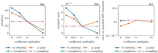
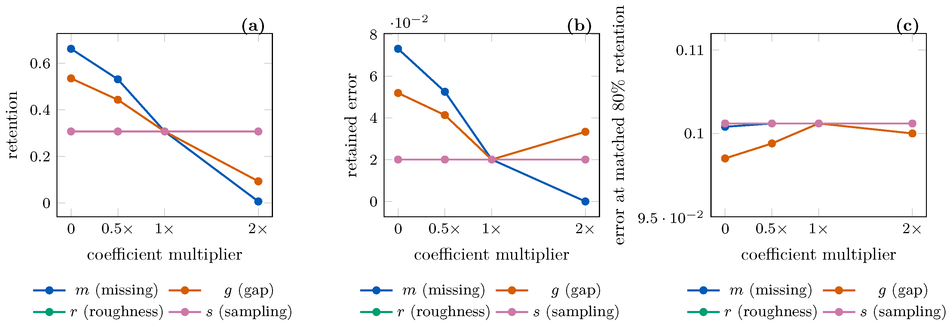
The coefficients were fixed before evaluation, not optimized on test error, and we do not claim a theoretical derivation for them. Their relative magnitudes encode a simple priority ordering: a fully missing observation ($m_i=1$) removes more information than a bounded 0.5-s gap, roughness twice the exercise-specific reference ($u_i=1$) signals corrupted kinematics, and sub-10 Hz sampling is the mildest degradation, hence $0.5>0.25>0.2>0.1$. Because the coefficients are heuristic, Section 4.4 reports a sensitivity analysis that varies each coefficient over $\{0,0.5\times ,1\times ,2\times \}$ while holding the others fixed; the qualitative conclusions (deferral under missingness and occlusion, no matched-retention benefit) are unchanged across the grid, and only the amount of deferral under missingness and occlusion responds to the missingness and gap weights. The score is not a probability and may fall below 0.5. It ranks observations by confidence and observable degradation. The sampling penalty activates below 10 Hz; tested 10 Hz and 15 Hz conditions receive no direct frequency penalty, although downsampling affects features and confidence.

The quality score is used for the predefined Forest. Other classifiers use maximum calibrated probability for their fixed reporting rule. These fixed-rule results are consequently properties of the entire stated pipeline, not a controlled comparison of classifier architecture with identical selectors. The main quality ablation is instead performed within the Forest using the four ranking variants: raw confidence, temperature confidence, raw confidence plus quality, and temperature confidence plus quality.

3.5. Fixed Thresholds and Matched-Retention Diagnostics

For each fold and model, the fixed reporting threshold is the 20th percentile of the applicable score among calibration observations. A test observation is retained if its score reaches that threshold. This targets approximately 80% calibration retention, not guaranteed 80% retention among new people. Test retention and classification error among retained observations are reported separately. A subject with zero retained predictions has undefined selective error, not zero error. The released per-subject tables preserve this distinction.

Matched-retention analyses answer a different descriptive question. For each subject and condition, observations are ordered by a score without consulting their labels, and exactly the highest-scoring 80% are retained for the diagnostic. Equal scores are resolved using fixed pseudorandom tie keys independent of labels, rather than archive order. Error-retention curves apply the same rule across retained fractions from 20% to 100%. These analyses do not provide a deployable threshold because they know the subject’s test-score distribution. They are not thresholds selected to minimize test error either: labels are used only after score-based selection to evaluate the retained decisions.

Under observation shift, a useful ranking can coexist with a threshold that rejects almost every prediction. A threshold can also retain confident but unreliable predictions. We assess retained error together with the retained fraction. The quality score is a heuristic input-quality indicator; it has no learned failure-probability interpretation or distribution-shift guarantee.

3.6. Paired Observation Perturbations

Perturbations are applied only to held-out observations after the models, training imputers, temperature parameters, and fixed thresholds have been fitted. Labels, person identifiers, exercise identifiers, and repetition identities are unchanged. Every model sees the same realization of a given corrupted repetition. Random generators use the specified corruption seed and a reproducible identifier-derived offset; correct and non-optimal repetitions with matching identifiers use the same seed convention. This pairing controls observation-error realizations across models without constructing additional ground-truth labels.

Angular noise adds independent zero-mean Gaussian errors at standard deviations of 2, 5, 10, and 20 degrees. Missingness masks a joint-frame with probability 0.1, 0.2, or 0.3 and removes all three components. These are mask probabilities; realized missing fractions vary between repetitions. Temporal occlusion masks 0.1, 0.3, or 0.5 s at a randomly selected feasible onset. It affects eight lower-body joints for exercises 1–6 and eight arm-region joints for exercises 7–10. Downsampling retains every second or third frame with its nominal timestamp. No anti-alias filter is applied, so this is a temporal-decimation stress test, not a validated simulation of a native lower-rate sensor. If the last source frame is omitted, recorded feature duration decreases by at most $(k-1)/30$ s for factor k.

The three stochastic families use seeds 1701, 1702, and 1703. Downsampling is deterministic. Together with the clean condition, there are 33 condition-and-seed realizations and 13 distinct severity levels including clean. Perturbed sequences are processed with the same bounded-gap interpolation and feature policy as clean sequences. The analysis does not retrain a corruption-specific model or recalibrate on perturbed test data. These are controlled errors in released local-rotation observations. They do not model image formation, correlated tracking failure, camera placement, Euler gimbal-lock behavior, clothing, lighting, or the physics of an occluded limb.

3.7. Metrics, Uncertainty Summaries, and Reproducibility

The primary metric is subject-balanced balanced accuracy: sensitivity and specificity are averaged within subject, then across the ten held-out subjects. Macro-F1, area under the receiver-operating-characteristic curve (AUC), raw and calibrated Brier scores, and calibrated log loss are secondary measures. Every metric is calculated within subject before aggregation. Selection metrics include fixed-threshold retention, conditional error among retained observations, and four matched-80% diagnostics. Thus, selective error is an equal-weight mean of subject-level conditional errors, not a pooled error weighted by the number retained.

Stochastic-seed metrics are first averaged within a subject at a severity level. Descriptive 95% intervals are then calculated from 2000 bootstrap resamples of the ten subject-level values. Repetitions, seeds, and folds are not additional independent units. We acknowledge that 2000 resamples of ten empirical points yield a discrete approximation of the sampling distribution, so the paper additionally reports Student-t intervals ($n=10$, $\mathrm{df}=9$, $t_{0.975}=2.262$) for all headline metrics; the two interval types agree closely (Table S5), and the bootstrap intervals are retained because they remain defined for degenerate distributions where the t interval collapses to a point (for example, 50.0% accuracy when every subject is predicted non-optimal). Leave-one-subject-out influence diagnostics accompany both. These intervals summarize test-participant variability conditional on the fixed folds, fitted models, temperatures, and thresholds. They do not propagate uncertainty from fitting on the two calibration participants or refitting overlapping training sets, and they cannot support population-level inference from ten participants. No multiplicity-adjusted superiority test or guaranteed coverage statement is reported. Displayed percentages use one decimal place after stabilizing binary floating-point values to 12 decimal places; paired differences explicitly use unrounded metrics.

After the predefined evaluation, a descriptive audit examined score saturation and the paired clean Brier change. These explanatory summaries use the unchanged predictions; they do not select models, tune quality weights, or revise thresholds.

3.8. Exploratory Post-Hoc Analyses

Three exploratory analyses were added after inspecting the initial results, are not part of the pre-fit protocol, and are hypothesis-generating rather than confirmatory: they suggest what a deployable adaptation mechanism might achieve, but they do not validate it. All preregistered-style frozen-rule results remain reported unchanged alongside them. First, we count the originally missing angular components filled by bounded interpolation, residual missingness, and changed feature vectors. We then disable sequence interpolation for every missingness and occlusion realization, while retaining the same fitted Forest and training-median feature imputer. This tests one preprocessing choice, not an alternative classifier trained for missing inputs.

Second, the same full Forest is evaluated with a confidence-only fixed rule. Its threshold is the 20th percentile of maximum temperature-scaled probability on the original clean calibration participants; no-duration models are not used as selector controls. Third, a severity-matched decision cutpoint is fitted to maximize balanced accuracy on the two calibration participants’ noisy records, pooling the three specified seeds. Ties select the cutpoint nearest 0.5, then the smaller value. The unmodified Forest’s raw probabilities are compared with this cutpoint on the separate test participants. This analysis requires known corruption severity and labeled shifted calibration recordings; it is neither an oracle cutpoint fitted to test labels nor an operational calibration guarantee. Because the cutpoint was chosen after seeing the primary results, it is presented as exploratory. AUC and all original frozen-rule results remain reported alongside it.

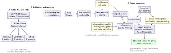
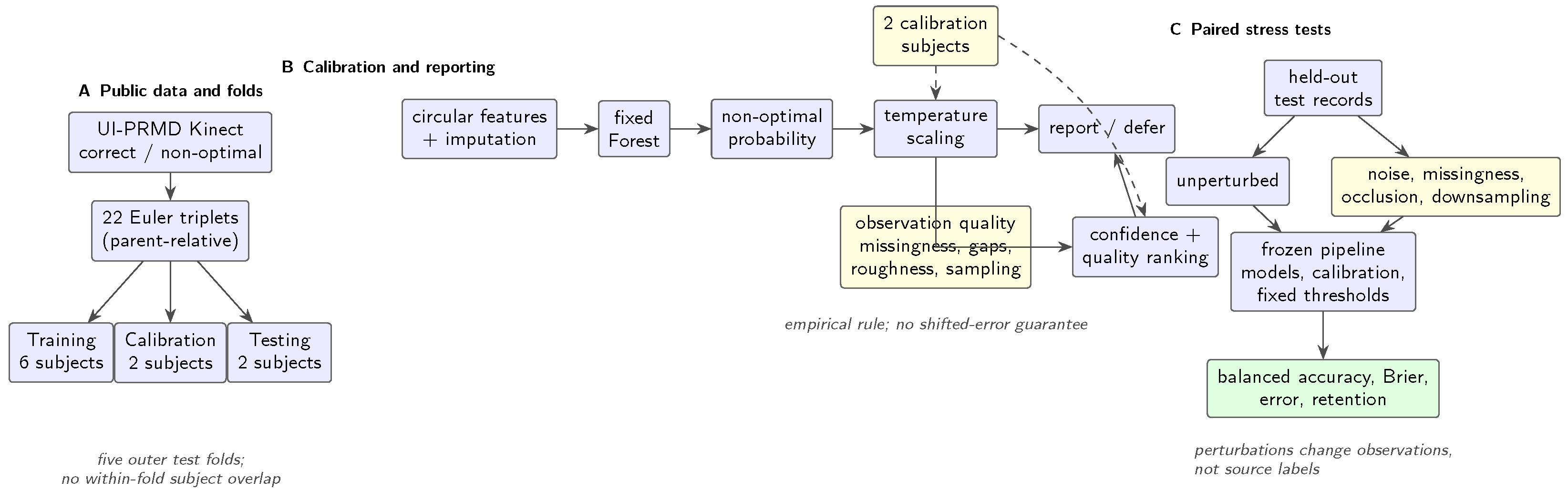
Supplementary Materials S1 contain the protocol, hashes, participant splits, fitted-model parameters, per-record predictions, subject metrics, software versions, and tests. Analysis used Python 3.11.9 (Python Software Foundation, Wilmington, DE, USA), with NumPy 2.4.6, SciPy 1.17.1, scikit-learn 1.9.0, pandas 3.0.3, and Matplotlib 3.11.0 (NumFOCUS, Austin, TX, USA) on Windows 10 with four logical processors; forests used two parallel workers. Tests cover actual angle-wrap crossings, masking and timestamps, fixed-seed splits, synthetic fitting and imputation, bootstrap and tie reproducibility, optimizer failure, and undefined selective error. These tests verify implementation properties, not population validity. Saved-model clean probabilities were checked against all 25 fitted-model exports. Figures are supplied as vector PDFs and 600-dpi PNGs; Figure 1 is a conceptual diagram, not an empirical image.

Figure 1. Audit pipeline. Participants are separated within each fold. Solid arrows show the processing flow; dashed arrows mark clean-calibration inputs for temperature and threshold. Blue boxes denote processing steps, yellow boxes observation-quality inputs, and the green box reported metrics. Labels carry no validated PE grading interpretation.

4. Results

4.1. Clean Generalization and Representation Diagnostics

The predefined Forest achieved 83.6 [79.5, 87.3]% mean participant-level balanced accuracy, 83.4% macro-F1, and an AUC of 0.922 (Table 3). Boosting reached 82.6 [79.6, 85.5]%; the primary model remained fixed throughout evaluation. The duration-only diagnostic reached 50.2 [45.1, 55.2]%. The no-duration forest obtained 83.7 [80.2, 87.0]%, an unrounded paired difference of 0.15 percentage points relative to the full Forest (descriptive 95% interval −1.15 to 1.30). Angular-speed summaries remain in this ablation, so removing the explicit duration feature leaves temporal information in the representation.

Table 3. Clean subject-independent classification. All metrics are means over subjects; brackets are descriptive 95% subject-bootstrap intervals. Brier scores are lower-is-better. Temperature scaling does not change binary decisions.

Model	Balanced Accuracy (%)	Macro-F1 (%)	AUC	Raw Brier	Cal. Brier
Prior	50.0 [50.0, 50.0]	33.3	0.500	0.250	0.250
Duration only	50.2 [45.1, 55.2]	46.5	0.482	0.254	0.253
Logistic	77.8 [72.9, 82.8]	77.6	0.864	0.180	0.152
Forest	83.6 [79.5, 87.3]	83.4	0.922	0.136	0.119
Boosting	82.6 [79.6, 85.5]	82.5	0.899	0.130	0.129
Forest, no duration	83.7 [80.2, 87.0]	83.6	0.921	0.136	0.119

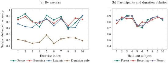
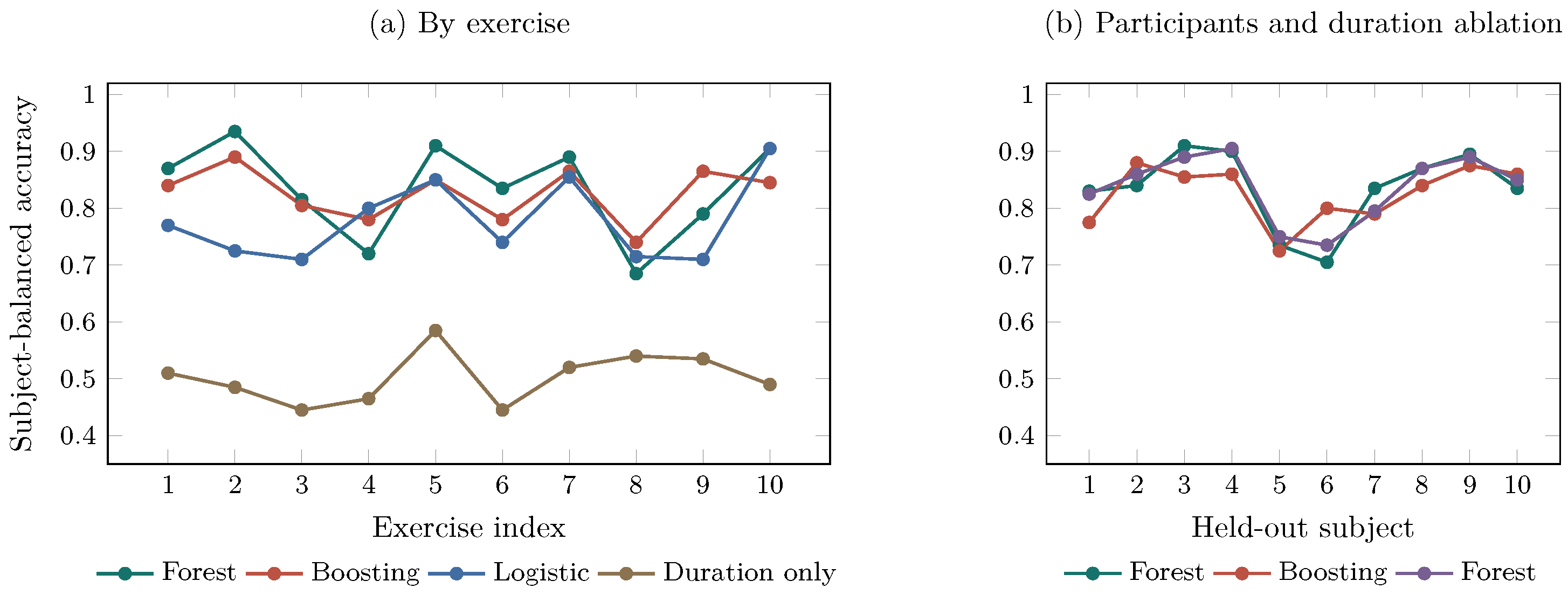
Figure 2 shows performance by exercise and by participant. Forest balanced accuracy ranged from 70.5% to 91.0% across held-out participants, each weighted equally in the overall mean. These comparisons apply to the five specified splits and fixed hyperparameters. No significance-tested ranking of movement-assessment architectures was performed.

Figure 2. Clean generalization from out-of-fold predictions. (a) Forest, Boosting, Logistic, and Duration only compare exercise-level performance; the last uses only elapsed duration. (b) Forest, Boosting, and Forest with the duration feature removed compare participant variation and the duration ablation; angular-speed features remain. The different model sets serve these two diagnostics. Exercise numbers follow Table 2; categorical connecting lines only guide the eye.

4.2. Calibration and Selective Classification

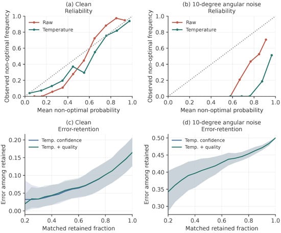
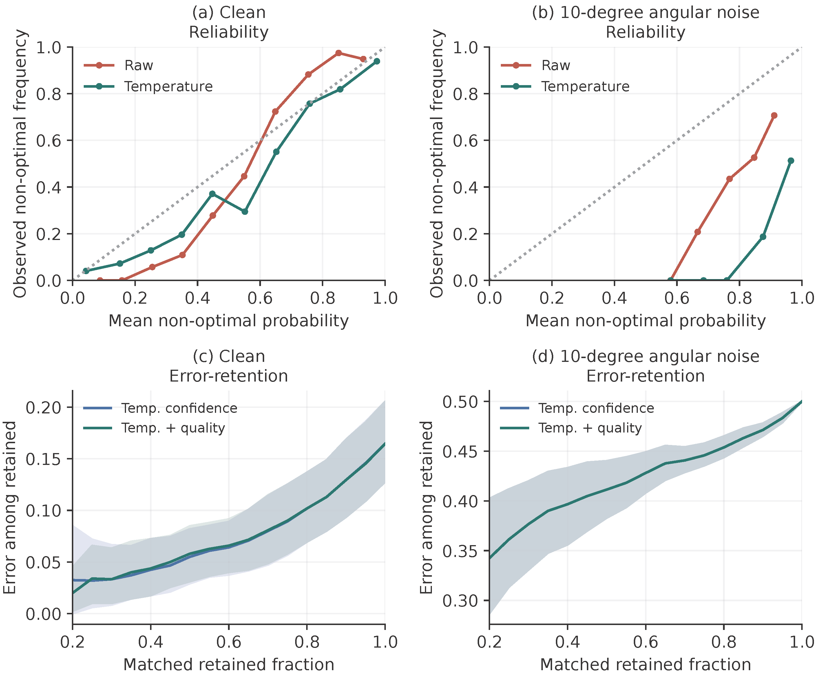
Temperature scaling reduced the clean Forest Brier score from 0.1356 to 0.1189; the paired calibrated-minus-raw difference was −0.0167 (conditional descriptive interval −0.0275 to −0.0043). Forest temperatures ranged from 0.317 to 0.699; values below one sharpen the clean model’s probabilities (Table S1). This interval describes test-participant variation with those temperatures fixed, not uncertainty in fitting calibration. Under 10-degree noise, raw and calibrated Brier scores were 0.3482 and 0.4581, reversing the clean improvement (Figure 3).

Figure 3. Forest reliability and matched-retention error: (a,c) clean; (b,d) 10-degree angular noise. Reliability diagrams use ten fixed-width bins; occupied-bin counts and repeated-record support are given in Table S3. Noisy pools contain three realizations per source record, not independent participants. “Temp. confidence” and “Temp. + quality” match Table 4; their noise curves overlap because the penalty is constant. Shading denotes pointwise descriptive participant-bootstrap intervals, not simultaneous bands. Fixed-rule thresholds are fitted separately on clean calibration participants.

At matched 80% retention, temperature confidence and temperature confidence plus quality both gave 10.2% clean error. The quality-aware fixed rule retained 79.4 [76.2, 82.7]%, with 10.0% mean participant-level conditional error. Table 4 separates matched ranking from two independently calibrated fixed rules on the same Forest. At mask probability 0.30, confidence alone retained 78.2% with 9.8% error, whereas quality-aware selection retained 30.5% with 2.7% error. The lower error accompanies substantially more deferral; it is not error control at equal reporting volume.

Table 4. Same-Forest selector controls. Values are percentages except the count of subjects with undefined quality-rule error. (a) Scores select exactly 80% within subject; temperature confidence has the same observed ordering as raw confidence. (b) Each rule has its own clean-calibration 20th-percentile threshold. Conditional errors are subject-weighted; zero-retention error is undefined, not zero.

(a) Error at matched 80% retention
Condition	Temp. Confidence		Raw + Quality		Temp. + Quality
Clean	10.2		10.2		10.2
Noise: 10 deg	45.4		45.4		45.4
Mask: 0.30	10.0		10.0		9.9
Gap: 0.5 s	10.6		10.7		10.6
Decimation: 10 Hz	12.6		12.6		12.6
(b) Fixed clean-calibration rules
	Temp. Confidence		Temp. + Quality
Condition	Retention	Error	Retention	Error	Undefined
Clean	79.4	9.9	79.4	10.0	0
Noise: 10 deg	99.8	49.9	54.0	–	4
Mask: 0.30	78.2	9.8	30.5	2.7	0
Gap: 0.5 s	78.7	10.5	24.3	4.1	0
Decimation: 10 Hz	75.8	11.1	75.8	11.1	0

The calibration percentile is a reporting target, not a model capability. On clean data, Prior retained 100.0% with 50.0% error because its tied score meets the threshold; Duration only retained 78.4% with 51.9% error. Reliability-bin counts and unique-record support are reported in Table S3 and the complete support CSV.

4.3. Observation Robustness

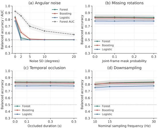
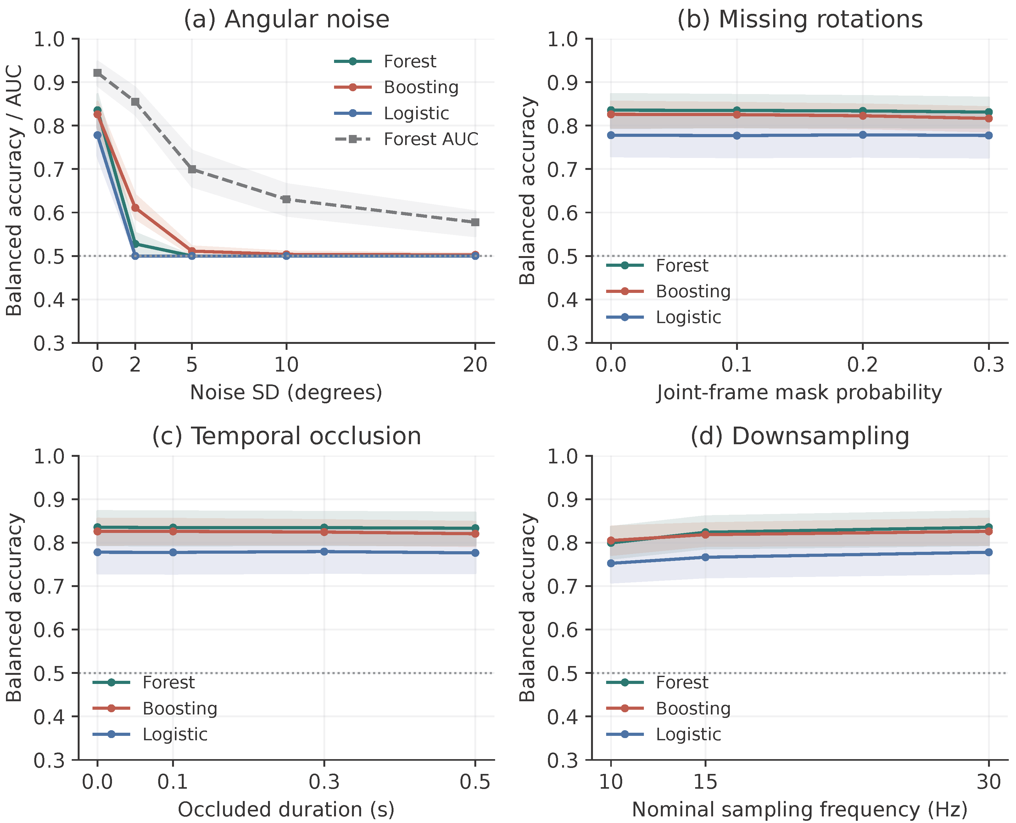
At just 2-degree independent angular noise, Forest balanced accuracy at the unchanged 0.5 cutpoint fell to 52.8 [50.6, 55.3]%, although AUC remained 0.855. At 5, 10, and 20 degrees, all Forest predictions were non-optimal, and balanced accuracy was 50.0% for every participant; AUC was 0.699, 0.630, and 0.577, respectively (Figure 4a; Table S2). Thus, binary-decision collapse does not mean all ranking information vanished. Increasing noise also reduced AUC relative to the clean value 0.922, so a cutpoint shift alone cannot explain every change. Under 20-degree noise, raw/calibrated Brier scores were 0.3280/0.4406, and quality-rule retention was 43.2%.

Figure 4. Frozen-pipeline stress tests. Forest, Boosting, and Logistic compare the three full-representation classifiers; all six predictors remain in the supplementary exports. (a) Also shows Forest AUC (dashed squares), separating ranking from decisions at 0.5. (b,c) Include the original bounded interpolation, not a bare-classifier missing-data test. Zero severity and 30 Hz are clean points. (d) Uses unfiltered decimation. Seeds are averaged within participant; bands are pointwise descriptive 95% intervals conditional on fitted pipelines. Intermediate severities were not tested.

The post-review, severity-matched cutpoint control achieved 77.0 [73.4, 81.3]% at 2 degrees and 54.7 [52.0, 57.0]% at 20 degrees. It used only noisy calibration participants to choose the decision cutpoint, without retraining the Forest. Its partial recovery identifies a cutpoint-sensitive component of failure; it neither restores clean ranking nor validates adaptation to unknown real sensor errors.

With the original interpolation policy, mask probability 0.30 gave 83.1 [79.5, 86.4]% balanced accuracy; bounded interpolation filled 95.1% of originally missing components on average. Only 0.0% of record realizations had no residual missing values, and 100.0% had altered features. Filling gaps therefore did not restore the original recording. Disabling sequence interpolation gave 83.4 [79.3, 87.1]% at the same mask probability. Thus, the observed stability did not require sequence interpolation in this control. For 0.5-s occlusion, the corresponding original and disabled-interpolation results were 83.3 [79.5, 86.9]% and 83.3 [79.5, 86.9]% (Table S4); these long gaps were not filled by either policy. Missing-aware summaries and training-median feature filling remained, so neither comparison establishes native classifier or camera robustness.

The original-policy paired changes from clean were −0.43 percentage points for mask probability 0.30 (conditional interval −1.32 to 0.43) and −0.22 for 0.5 s occlusion (−0.63 to 0.22). Quality-rule retention was 30.5% and 24.3%, respectively. Decimation to nominal 10 Hz gave 80.0 [76.4, 83.6]% accuracy and 75.8% retention. The original fitted models and rules remain unchanged.

Under 10-degree noise, four participants had zero quality-rule retention in all three seeds, leaving their fixed-rule error and the aggregate error undefined. The noise quality penalty was exactly 0.25 for every tested record and severity, so it preserved confidence ordering while changing threshold crossings. Temperature scaling likewise cannot move the binary 0.5 cutpoint.

4.4. Sensitivity and Diagnostics

4.4.1. Deferral-Score Coefficient Sensitivity

Each quality coefficient was varied over $\{0,0.5\times ,1\times ,2\times \}$ of its baseline value while the others were held fixed, with the original frozen per-fold thresholds retained (Figure 5). Matched-80% retention error was essentially flat across the entire grid in every condition (the within-condition span never exceeded 0.003; for example, 0.099–0.101 at 30% missingness), confirming that the penalty’s ranking contribution is marginal. Under the frozen thresholds, only the missingness and gap weights changed the deferral behaviour materially: doubling the missingness weight ($m=1.0$) pushed retention at 30% missingness from 30.5% to 0.7%, while zeroing it ($m=0$) raised retention to 66.2% with error rising from 2.7% to 7.3%. The roughness and sampling weights had almost no effect outside the angular-noise conditions, where roughness saturation makes the weight a constant shift. These results locate the score’s sensitivity in the two coefficients that govern missing-data deferral and show that the reported error–retention trade-offs are representative of the intermediate weight choices rather than artifacts of the exact baseline values.

Figure 5. Sensitivity of the quality-aware rule to its coefficients, evaluated under 30% missingness with the original frozen per-fold thresholds. (a) Retention and (b) retained conditional error as each coefficient varies over zero, half, once, and twice its baseline value; (c) error at matched 80% retention, which is flat across the entire grid.

4.4.2. Temperature Stability Across Folds

The five fitted Forest temperatures span 0.317–0.699. Exchanging each fold’s temperature with every other fold’s temperature changes the clean calibrated Brier score by at most 0.017 (mean absolute change 0.008), comparable in scale to the calibration improvement itself ($-0.0167$). The calibration results are therefore not dominated by the idiosyncrasies of one calibration pair, although this exchange analysis cannot rule out sensitivity to shared characteristics of the two-subject calibration design.

4.4.3. Small-Sample Intervals and Influence

Student-t intervals agree closely with the bootstrap intervals for all headline metrics (clean balanced accuracy 78.7–88.4% vs. 79.5–87.3%; Table S5). Leave-one-subject-out influence on the clean balanced accuracy is at most 1.7 percentage points (removing subject 6 raises it), and no single participant drives the noise or missingness conclusions (max influence 1.6 points; Table S6).

4.4.4. Probability-Distribution Diagnostics

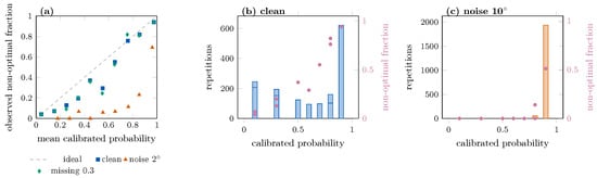
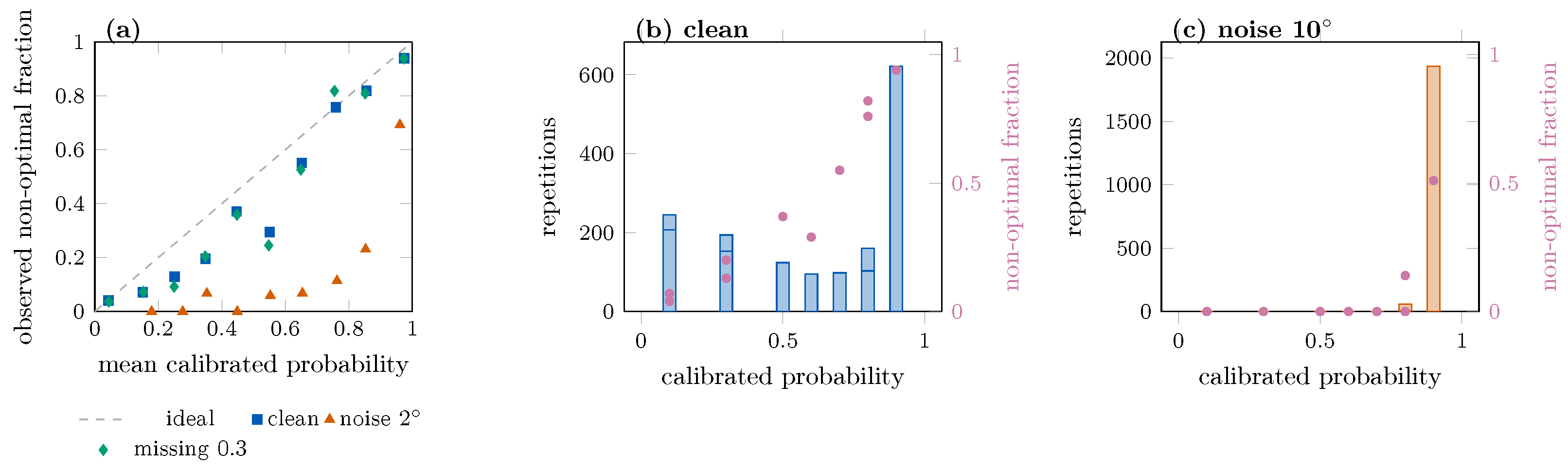
Ten-bin expected calibration error (ECE) quantifies the reliability diagrams: ECE grows from 0.068 (clean) to 0.392 at 2-degree noise and 0.461 at 10 degrees, while remaining below 0.11 under all missingness, occlusion, and downsampling conditions. This separates the failure layers explicitly: probability quality collapses under noise together with the decision rule, while it degrades only mildly under missing-data conditions whose decisions remain accurate. Under 10-degree noise, the calibrated probabilities bunch near 0.5 and 1.0, while the empirical non-optimal fraction in the high-confidence bins stays near 0.5, which is the signature of confidently wrong predictions (Figure 6).

Figure 6. Probability-distribution diagnostics for the calibrated Forest. (a) Ten-bin reliability of the seed-averaged calibrated probabilities under clean, 2-degree noise, and 30% missingness conditions; (b,c) calibrated-probability histograms with the empirical non-optimal fraction per bin (right axes) under clean and 10-degree noise conditions. In (a), squares, triangles, and diamonds mark the clean, 2-degree-noise, and 30%-missingness conditions, and the dashed line marks ideal calibration; in (b,c), bars show repetition counts (left axes) and dots the empirical non-optimal fraction per bin (right axes). Under noise, the high-confidence bins contain near-chance error rates.

4.4.5. Paired Tests

Wilcoxon signed-rank tests over the ten subjects support the main paired claims: clean calibration improvement (mean Brier change $-0.0167$, $p=0.047$, sign test $p=0.021$) and the exploratory cutpoint adaptation at every noise level (all $p\le 0.017$). The interpolation on/off difference at 30% missingness is not significant ($p=0.33$), consistent with the interpretation that interpolation is immaterial rather than that a small difference was missed.

4.5. Kinematic Phase Profiles

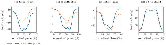
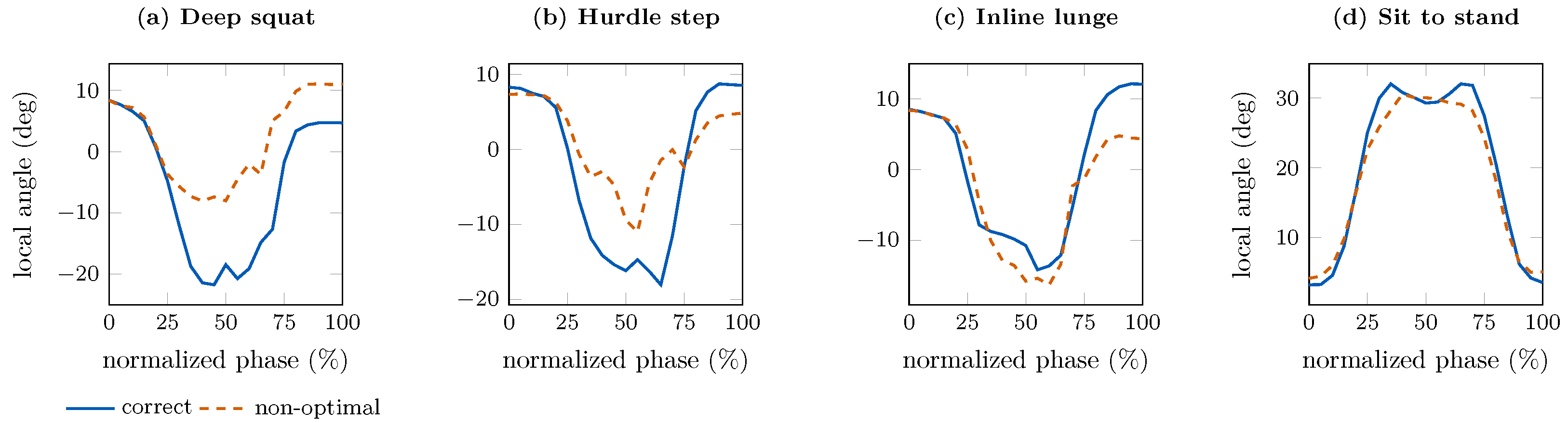
To connect the audited representation to movement kinematics, we analyzed phase profiles of the released raw Kinect Euler angles. For each exercise, the dominant Euler component was selected among the right and left upper-leg joints (exercises 1–6) or the upper-arm joints (exercises 7–10) as the component with the largest median range of motion in the correct class (26–38 degrees; Table S8). Each repetition was time-normalized to a common phase axis of 21 samples, and per-participant mean profiles, peak angles, times of peak, and ranges of motion were computed for each class (Figure 7).

Figure 7. Time-normalized mean phase profiles of the dominant local Euler component per exercise: (a) deep squat; (b) hurdle step; (c) inline lunge; (d) sit to stand. Solid lines: correct; dashed lines: non-optimal; profiles are averaged within participant and then across the ten participants. The dominant component was selected by median range of motion in the correct class; angles are parent-relative local rotations, not anatomical flexion angles.

The profiles show that the deliberately non-optimal executions differ from correct ones mainly in movement amplitude and timing rather than in phase shape. In the lower-body exercises, non-optimal repetitions of the dominant lower-leg component reach systematically smaller ranges of motion: the correct-minus-non-optimal difference is 20.2 degrees (SD 24.4) in the deep squat, 27.1 (32.3) in the hurdle step, 20.8 (24.5) in the inline lunge, and 10.0 (29.1) degrees in the side lunge, with the deep-squat descent reaching roughly half the correct amplitude. Sit-to-stand and straight-leg-raise differences are small (1.9 and 5.3 degrees). In the shoulder exercises, ranges of motion are similar between classes ($-1.5$ to $4.0$ degrees), and the classes separate instead on peak angle (differences of 4–8 degrees) and time of peak (for example, shoulder scaption peaks near 33% of the movement in correct repetitions and near 67% in non-optimal ones). These descriptors are exactly the quantities that the bag-of-frames summaries retain (range, mean level, and speed statistics), which is consistent with the observed clean separability and with the exercises’ uneven difficulty.

The interpretation is bounded by the release. The analyzed quantities are parent-relative local Euler components, not anatomical flexion angles: the release does not document the coordinate reconstruction needed to compute joint flexion from the local rotations and positions, so we describe phase profiles of the released local rotations rather than anatomical joint angles. The analysis is also descriptive and outcome-free: it characterizes what the two label classes look like in the raw observations and does not validate a biomechanical phase model or an error taxonomy.

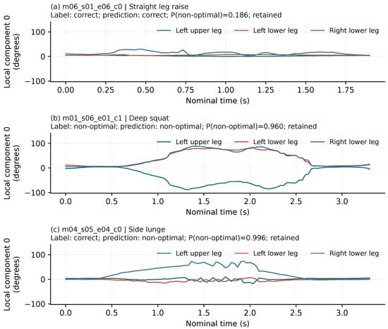
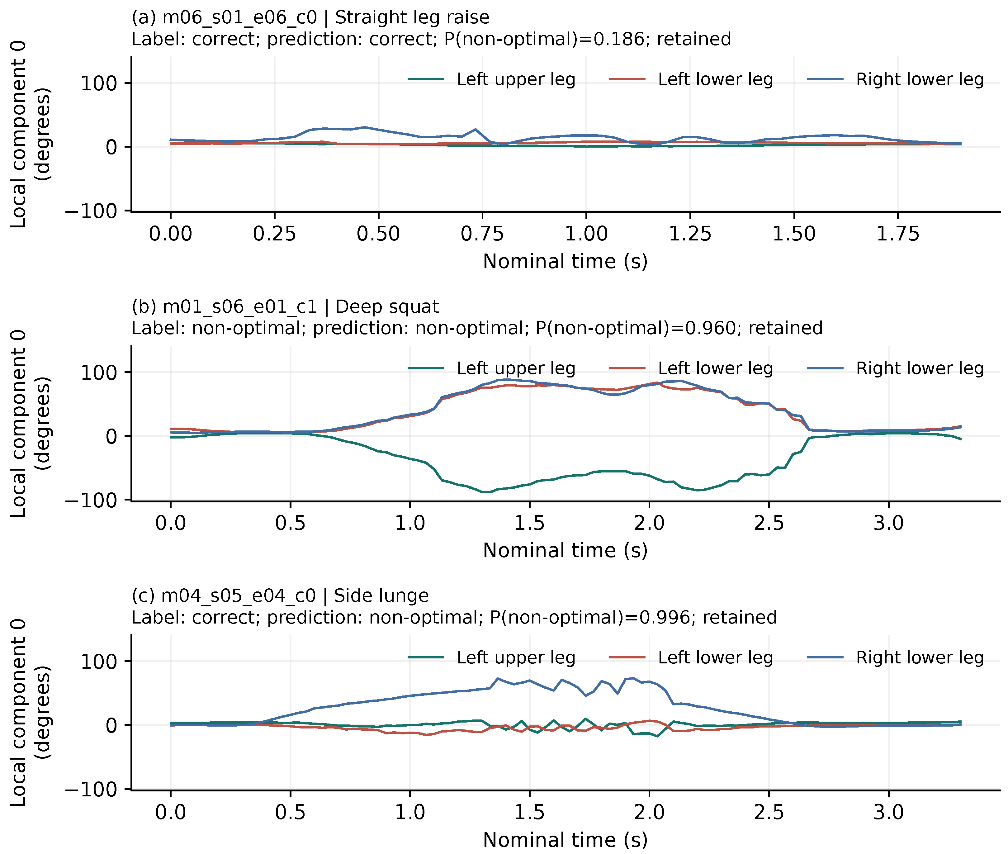
4.6. Inspectable Cases and Computation

Figure 8 shows two correctly classified clean repetitions and one failure. The first two occupy the median calibrated-confidence rank within their correctly classified source classes. The failure is the highest-confidence erroneous clean Forest prediction; ties are resolved by record identifier. Selection uses the observed outcomes for illustration only; the exported identifiers and probabilities make it auditable.

Figure 8. Outcome-selected clean cases, with common angle limits across panels. (a) Straight-leg-raise repetition from the median-confidence correctly classified correct class; (b) deep-squat repetition from the median-confidence correctly classified non-optimal class; (c) the highest-confidence clean error, a correctly labeled side-lunge repetition predicted non-optimal. Traces show unwrapped parent-relative Euler component zero of the named joints against nominal time, not global skeletons or instructional correction labels. “Retained” refers to the fixed clean-calibration quality threshold; all three cases were retained, including the error in (c). The cases illustrate inspection and do not validate a causal interpretation.

Each case displays Euler component zero of an upper-leg and two lower-leg joints, a display choice fixed for these lower-body cases. The three panels share one vertical scale for comparison. The confident error was retained by the reporting rule despite a finite clean input sequence.

Forest fitting took a mean of 3.45 s across folds. Probability scoring in batches of 400 averaged 0.3266 ms per repetition; logistic regression and boosting averaged 0.0411 and 0.0710 ms. Acquisition, segmentation, feature extraction, network transfer, and interface overhead were excluded, so these timings say nothing about end-to-end latency or real-time classroom deployment.

5. Discussion

5.1. Interpretation of the Stress Test

The released local rotations supported classification of unseen participants under clean conditions. Under angular noise, the fixed 0.5 decision rule collapsed earlier than the ranking became uninformative. AUC nevertheless declined with severity. The calibration-only cutpoint control partly separates these two effects without selecting a cutpoint on test labels. It depends on labeled, severity-matched calibration data, so it does not establish a correction for an unknown real-world shift.

The duration-only model and no-duration forest test the contribution of the explicit duration feature. Deliberate non-optimal recordings could contain timing or acquisition cues that correlate with the labels. Removing duration leaves angular-speed summaries and other possible cues in place. The ablation therefore cannot establish a biomechanical explanation for the model’s decisions. That would require additional annotations and controlled recording conditions.

The six-predictor comparison uses fixed hyperparameters and one participant partition, not exhaustive tuning. Table 5 places our clean results next to published UI-PRMD and KIMORE results. The comparison is indicative only: Liao et al. predict derived continuous scores from a reduced Vicon release with a random 70/30 split [27]; recent studies report quality-assessment errors (MAD) on different targets and protocols [24], with the strongest current contrastive-learning result reporting UI-PRMD accuracy 0.997 [23]. None of these studies perturbs the observations, so they cannot be compared on robustness at all; our 83.6% participant-separated clean accuracy is consistent with the difficulty level of the binary correctness task. No published-score or state-of-the-art superiority claim follows from this analysis, and the table’s purpose is to position the audit, not to benchmark it.

Table 5. Indicative quantitative comparison with recent published results on the same public datasets. Targets, sensors, and validation protocols differ across rows, so values are not directly comparable; robustness columns are absent for prior work because controlled observation degradation has not been evaluated there. MAD: mean absolute deviation against clinical scores.

Study	Data/Target	Clean Result	Robustness Tested
Liao et al. [27] (2020)	UI-PRMD (Vicon), quality score	MAD 0.13 (random split)	No
Raihan et al. [24] (2025)	UI-PRMD + KIMORE, correctness/quality	UI-PRMD MAD 0.014	No
Karlov et al. [23] (2025)	UI-PRMD, IRDS, KIMORE, quality	UI-PRMD accuracy 0.997 (3:1 split)	No
Kourbane et al. [21] (2025)	UI-PRMD, binary correctness	98.6% (random split)	No
Present audit	UI-PRMD (Kinect), binary correctness	83.6% (participant-separated)	Yes (4 degradation families)

5.2. Calibration and Reporting Under Observation Shift

Positive temperature scaling changes probability sharpness while preserving the binary decision. Its monotonic transformation also explains the equal raw- and temperature-confidence matched-retention errors observed for the primary Forest. Calibration can affect probability interpretation and fixed-threshold behavior without changing ranking. Conversely, a favorable clean Brier score does not imply calibrated probabilities under observation degradation.

The quality score measures observable degradation, which does not uniquely determine classifier error. Missingness and gaps are detectable from the input. Roughness is ambiguous because both noise and genuine fast movement can increase it; an exercise-specific training reference only partly addresses this problem. The fixed coefficients have no causal injury or error interpretation. We retained them throughout evaluation, including when the penalty failed to improve ranking or caused excessive deferral.

The quality penalty showed no consistent matched-retention advantage. Its lower fixed-rule error under missingness came with substantially fewer reported predictions than the same-Forest confidence rule. This is an error–retention trade-off, not an operating guarantee. Input-quality penalties respond to missingness recorded before interpolation, whereas the classifier uses processed summaries. Deferral can therefore remain high when preprocessing preserves classification accuracy; neither curve alone describes the full reporting cost.

At every tested angular-noise level, roughness exceedance reached its cap for every record and the other penalties were zero. The score reduced to $s_i=\max (p_i^{\left(T\right)},1-p_i^{\left(T\right)})-0.25$. Subtracting this constant changes threshold crossings but preserves ordering. Saturation also removes the penalty’s ability to distinguish these noise severities. Independent framewise noise alters angular-speed summaries, so the result applies to this representation and corruption model; it does not estimate the failure rate of a physical camera system.

Matched-retention error isolates ordering by imposing the same reporting budget on each score. A fixed calibration threshold instead tests a rule that can be applied without access to test-score quantiles. Under observation shift, that rule may retain far fewer predictions or report more errors. Zero retention leaves selective accuracy undefined. Complete deferral may be appropriate for inadequate observations, but it supplies no movement classifications.

5.3. Implications for AI Integration in Physical Education

The audit speaks to a specific question in AI-in-education research: what must hold before an automated assessment component is handed to teachers? Reviews of AI in education emphasize that adoption depends on teacher agency, transparency, and human oversight rather than raw model accuracy [3]. The quality-aware deferral rule operationalizes one part of that principle: when the observation stream degrades, the system withholds its judgment and routes the decision back to the teacher, who sees the withheld fraction and the observation-quality indicators rather than a silently degraded score. In this reading, deferral functions as a teacher-in-the-loop interface property, and the audit quantifies its cost: under 30% missingness, the rule defers roughly 70% of predictions to achieve 2–3% retained error.

Higher PE motivated this technical audit, but the audit supplies reliability evidence, not educational evidence. Graduate students and faculty performing rehabilitation-oriented exercises are not a PE class, and deliberate non-optimal performances need not represent natural mistakes. The label gap matters for more than external validity. Natural student errors are unbalanced (a few dominant error types); embedded in variable clothing, occlusion, and camera placement; and graded against curricular criteria rather than a binary correct/non-optimal label. Moving from deliberate to natural errors is therefore a distribution-shift problem, not a data-volume problem: a classifier trained on deliberate errors can inherit decision boundaries tied to the way those errors were produced. Any transfer study must first establish label agreement between teachers and the collection protocol on the same recordings, because without that agreement, no clean test of the classifier under natural conditions exists. A future teacher-reviewed interface could expose observation quality, source-label meaning, and withheld predictions. Before instructional use, curricular grading criteria, teacher agreement, feedback utility, accessibility, fairness, and learner outcomes need independent evaluation. No teachers, feedback intervention, grades, learning gains, or workload changes were studied here.

Temporal-Ordering Limitation of the Representation

The sequence-summary representation is a bag of frames: it collapses each angular component to static statistics and largely discards the order of flexion and extension. Human movement is spatiotemporal, and in rehabilitation and PE contexts, the sequencing of joint flexion and extension is often itself the marker of non-optimal execution (for example, descending before the knees travel forward in a squat). Part of the noise-induced failure observed here may therefore stem from this representation choice rather than from sensor degradation alone: independent framewise noise corrupts angular-velocity statistics that are the representation’s main temporal channel. Disentangling the two requires sequence-aware architectures [21,23] evaluated under the same participant-separated perturbation protocol, which is a central next step.

5.4. Limitations and Next Validation Steps

Only ten independent people were available, including two calibration participants per fold. The many repetitions provide no substitute for a larger participant sample, and the 400 calibration repetitions are highly correlated within subject, so the effective calibration sample size is two people. The intervals describe participant-level variation conditional on fixed folds and overlapping training sets; another partition could give different results. Both the bootstrap intervals and the supplementary t intervals estimate variance from ten points, which is a severe constraint: they quantify dispersion in this sample, not the population sampling distribution, and they do not propagate uncertainty from the two-subject calibration fit (the cross-fold temperature exchange bounds that component at roughly 0.017 Brier units). They provide neither population-wide operating guarantees nor a precise failure rate for an unseen institution, and conclusions should be read as dataset-specific until replicated on a larger cohort.

The labels record intended correctness in healthy volunteers. They contain no blinded clinical ratings, PE achievement criteria, or independently annotated reasons for non-optimal performance. They cannot support injury-risk inference, anatomical error explanations, or validation of a continuous quality score. Transfer to clinical populations, other ages, abilities, exercises, or native video capture remains untested.

The representation and corruption models simplify the measurement process. Independent Euler-component errors differ from perturbations of a full three-dimensional rotation, and nominal timestamps omit sampling jitter and dropped acquisition frames. The disabled-interpolation control showed that stable missing-data classification did not require sequence interpolation in these tests. Missing-aware summaries and training-median feature filling remained in both pipelines, however, so this does not isolate an inherently missingness-robust classifier. Downsampling changes adjacent samples, can shorten nominal duration, and can affect unwrapping. Local-angle summaries also discard temporal order and may retain recording-protocol cues. External validation must include natural sensing failures: the tested independent errors, including 2-degree noise, are not an empirically measured Kinect noise model.

The quality score and bounded temperature model are empirical choices. Neither is an optimized uncertainty estimator, and the reporting threshold depends on the clean calibration population. Retained-error control after distribution shift has no theoretical guarantee here. Further testing could use a larger independent public dataset, repeated grouped partitions, and a preregistered external protocol without necessarily collecting new participant data. Revised models or thresholds would require new held-out evaluation data.

6. Conclusions

This study delivered a reproducible, participant-separated reliability audit of a fixed movement-classification pipeline on public UI-PRMD Kinect data, separating ranking quality, fixed-threshold decisions, and probability calibration. Its scientific novelty is the audit design itself: a controlled four-family degradation protocol on unchanged labels that shows different pipeline layers failing at different severities, a result invisible to clean-data accuracy comparisons. On this stress test, the predefined Forest achieved 83.6% clean balanced accuracy, and temperature scaling reduced the mean Brier score from 0.1356 to 0.1189. At 2-degree independent angular noise, fixed-cutpoint accuracy fell to 52.8%, while AUC remained 0.855; single-class decisions began at 5 degrees, and more severe noise also degraded ranking. Exploratory calibration-only cutpoint adaptation addresses part of the decision failure, whereas positive temperature scaling cannot move the 0.5 cutpoint. Classification of perturbed repetitions whose features were rebuilt from missing-aware summaries and fitted feature filling remained stable, but the classifier was never tested on natively missing inputs, so this is post-imputation stability, not native missing-data robustness. Quality-aware deferral trades reporting volume for retained error and is the component we interpret as a teacher-review trigger in future PE deployments. Practically, the audit provides education researchers with a released, seeded protocol for auditing any movement classifier before classroom use. These findings concern a controlled computational pipeline, not robustness of a physical sensor or validated PE grading. Independent sensing and educational validation remain necessary before instructional deployment.

References

- Hu, Z.; Liu, Z.; Su, Y. AI-Driven Smart Transformation in Physical Education: Current Trends and Future Research Directions. Appl. Sci. 2024, 14, 10616. [Google Scholar] [CrossRef] [Scilit]
- Tohănean, D.I.; Vulpe, A.M.; Mijaica, R.; Alexe, D.I. Embedding Digital Technologies (AI and ICT) into Physical Education: A Systematic Review of Innovations, Pedagogical Impact, and Challenges. Appl. Sci. 2025, 15, 9826. [Google Scholar] [CrossRef] [Scilit]
- Zhou, T.; Wu, X.; Wang, Y.; Wang, Y.; Zhang, S. Application of artificial intelligence in physical education: A systematic review. Educ. Inf. Technol. 2024, 29, 8203–8220. [Google Scholar] [CrossRef] [Scilit]
- Gao, Y. The role of artificial intelligence in enhancing sports education and public health in higher education: Innovations in teaching models, evaluation systems, and personalized training. Front. Public Health 2025, 13, 1554911. [Google Scholar] [CrossRef] [Scilit] [PubMed]
- Zhang, L.; Gao, J.; Zhao, L.; Liu, Z.; Guan, A. Predicting College Student Engagement in Physical Education Classes Using Machine Learning and Structural Equation Modeling. Appl. Sci. 2025, 15, 3884. [Google Scholar] [CrossRef] [Scilit]
- Zhang, L.; Liu, Z.; Zhao, L.; Gao, J. The Impact of Digital Technology Use on Teaching Quality in University Physical Education: An Interpretable Machine Learning Approach. Appl. Sci. 2025, 15, 7689. [Google Scholar] [CrossRef] [Scilit]
- Liu, C.; Yang, F.; Ge, C.; Shao, Z. A Dynamic Precision Evaluation System for Physical Education Classroom Teaching Behaviors Based on the CogVLM2-Video Model. Appl. Sci. 2025, 15, 7712. [Google Scholar] [CrossRef] [Scilit]
- Zawacki-Richter, O.; Marín, V.I.; Bond, M.; Gouverneur, F. Systematic review of research on artificial intelligence applications in higher education – where are the educators? Int. J. Educ. Technol. High. Educ. 2019, 16, 39. [Google Scholar] [CrossRef] [Scilit]
- Lee, H.S.; Lee, J. Applying Artificial Intelligence in Physical Education and Future Perspectives. Sustainability 2021, 13, 351. [Google Scholar] [CrossRef] [Scilit]
- Wu, C.H.; Wu, T.C.; Lin, W.B. Exploration of Applying Pose Estimation Techniques in Table Tennis. Appl. Sci. 2023, 13, 1896. [Google Scholar] [CrossRef] [Scilit]
- Rosique, F.; Losilla, F.; Navarro, P.J. Applying Vision-Based Pose Estimation in a Telerehabilitation Application. Appl. Sci. 2021, 11, 9132. [Google Scholar] [CrossRef] [Scilit]
- Cao, Z.; Hidalgo, G.; Simon, T.; Wei, S.E.; Sheikh, Y. OpenPose: Realtime Multi-Person 2D Pose Estimation Using Part Affinity Fields. IEEE Trans. Pattern Anal. Mach. Intell. 2021, 43, 172–186. [Google Scholar] [CrossRef] [Scilit] [PubMed]
- Kim, J.W.; Choi, J.Y.; Ha, E.J.; Choi, J.H. Human Pose Estimation Using MediaPipe Pose and Optimization Method Based on a Humanoid Model. Appl. Sci. 2023, 13, 2700. [Google Scholar] [CrossRef] [Scilit]
- Uhlrich, S.D.; Falisse, A.; Kidziński, L.; Muccini, J.; Ko, M.; Chaudhari, A.S.; Hicks, J.L.; Delp, S.L. OpenCap: Human movement dynamics from smartphone videos. PLoS Comput. Biol. 2023, 19, e1011462. [Google Scholar] [CrossRef] [Scilit] [PubMed]
- Zhang, H.B.; Cai, J.J.; Qiu, H.M.; Lei, Q.; Liu, J.H.; Zhang, M.H. A survey of deep learning-based action quality assessment: Methods and applications. J. Big Data 2026, 13, 70. [Google Scholar] [CrossRef] [Scilit]
- Liu, Y.; Qiu, C.; Zhang, Z. Deep learning for 3D human pose estimation and mesh recovery: A survey. Neurocomputing 2024, 596, 128049. [Google Scholar] [CrossRef] [Scilit]
- Vakanski, A.; Jun, H.P.; Paul, D.; Baker, R. A Data Set of Human Body Movements for Physical Rehabilitation Exercises. Data 2018, 3, 2. [Google Scholar] [CrossRef] [Scilit] [PubMed]
- Chander, A.; Bathula, D.R.; Sahani, A.K. Towards an RGB camera-based rehabilitation exercise assessment using an enhanced spatio-temporal transformer framework. Multimed. Tools Appl. 2025, 84, 48283–48307. [Google Scholar] [CrossRef] [Scilit]
- Sardari, F.; Paiement, A.; Hannuna, S.; Mirmehdi, M. VI-Net—View-Invariant Quality of Human Movement Assessment. Sensors 2020, 20, 5258. [Google Scholar] [CrossRef] [Scilit] [PubMed]
- Deb, S.; Islam, M.F.; Rahman, S.; Rahman, S. Graph Convolutional Networks for Assessment of Physical Rehabilitation Exercises. IEEE Trans. Neural Syst. Rehabil. Eng. 2022, 30, 410–419. [Google Scholar] [CrossRef] [Scilit] [PubMed]
- Kourbane, I.; Papadakis, P.; Andries, M. Optimized assessment of physical rehabilitation exercises using spatiotemporal, sequential graph-convolutional networks. Comput. Biol. Med. 2025, 186, 109578. [Google Scholar] [CrossRef] [Scilit] [PubMed]
- He, T.; Chen, Y.; Wang, L.; Cheng, H. An Expert-Knowledge-Based Graph Convolutional Network for Skeleton-Based Physical Rehabilitation Exercises Assessment. IEEE Trans. Neural Syst. Rehabil. Eng. 2024, 32, 1916–1925. [Google Scholar] [CrossRef] [Scilit] [PubMed]
- Karlov, M.; Abedi, A.; Khan, S.S. Rehabilitation exercise quality assessment through supervised contrastive learning with hard and soft negatives. Med. Biol. Eng. Comput. 2025, 63, 15–28. [Google Scholar] [CrossRef] [Scilit] [PubMed]
- Raihan, M.J.; Ahad, M.A.R.; Nahid, N. A deep learning model with interpretable squeeze-and-excitation for automated rehabilitation exercise assessment. Med. Biol. Eng. Comput. 2025, 63, 2871–2887. [Google Scholar] [CrossRef] [Scilit] [PubMed]
- Gupta, N.S.; Ramya, K.B.; Karnati, R. A Review Work: Human Action Recognition in Video Surveillance Using Deep Learning Techniques. Inform. Autom. 2024, 23, 436–466. [Google Scholar] [CrossRef] [Scilit]
- Capecci, M.; Ceravolo, M.G.; Ferracuti, F.; Iarlori, S.; Monteriù, A.; Romeo, L.; Verdini, F. The KIMORE Dataset: KInematic Assessment of MOvement and Clinical Scores for Remote Monitoring of Physical REhabilitation. IEEE Trans. Neural Syst. Rehabil. Eng. 2019, 27, 1436–1448. [Google Scholar] [CrossRef] [Scilit] [PubMed]
- Liao, Y.; Vakanski, A.; Xian, M. A Deep Learning Framework for Assessing Physical Rehabilitation Exercises. IEEE Trans. Neural Syst. Rehabil. Eng. 2020, 28, 468–477. [Google Scholar] [CrossRef] [Scilit] [PubMed]
- Halilaj, E.; Rajagopal, A.; Fiterau, M.; Hicks, J.L.; Hastie, T.J.; Delp, S.L. Machine learning in human movement biomechanics: Best practices, common pitfalls, and new opportunities. J. Biomech. 2018, 81, 1–11. [Google Scholar] [CrossRef] [Scilit]
- Zhou, Y.; Shao, W.D.; Wang, L. Effects of Feedback on Students’ Motor Skill Learning in Physical Education: A Systematic Review. Int. J. Environ. Res. Public Health 2021, 18, 6281. [Google Scholar] [CrossRef] [Scilit] [PubMed]
- Lander, N.; Nahavandi, D.; Mohamed, S.; Essiet, I.; Barnett, L.M. Bringing objectivity to motor skill assessment in children. J. Sport. Sci. 2020, 38, 1539–1549. [Google Scholar] [CrossRef] [Scilit]
- Ceriola, L.; Taborri, J.; Donati, M.; Rossi, S.; Patanè, F.; Mileti, I. Comparative Analysis of Markerless Motion Capture Systems for Measuring Human Kinematics. IEEE Sens. J. 2024, 24, 28135–28144. [Google Scholar] [CrossRef] [Scilit]
- Kanko, R.M.; Laende, E.; Selbie, W.S.; Deluzio, K.J. Inter-session repeatability of markerless motion capture gait kinematics. J. Biomech. 2021, 121, 110422. [Google Scholar] [CrossRef] [Scilit] [PubMed]
- Kanko, R.M.; Laende, E.K.; Davis, E.M.; Selbie, W.S.; Deluzio, K.J. Concurrent assessment of gait kinematics using marker-based and markerless motion capture. J. Biomech. 2021, 127, 110665. [Google Scholar] [CrossRef] [Scilit] [PubMed]
- Scott, B.; Seyres, M.; Philp, F.; Chadwick, E.K.; Blana, D. Healthcare applications of single camera markerless motion capture: A scoping review. PeerJ 2022, 10, e13517. [Google Scholar] [CrossRef] [Scilit] [PubMed]
- Desmarais, Y.; Mottet, D.; Slangen, P.; Montesinos, P. A review of 3D human pose estimation algorithms for markerless motion capture. Comput. Vis. Image Underst. 2021, 212, 103275. [Google Scholar] [CrossRef] [Scilit]
- Baldinger, M.; Reimer, L.M.; Senner, V. Influence of the Camera Viewing Angle on OpenPose Validity in Motion Analysis. Sensors 2025, 25, 799. [Google Scholar] [CrossRef] [Scilit] [PubMed]
- Hellstén, T.; Arokoski, J.; Karlsson, J.; Ristolainen, L.; Kettunen, J. Reliability and validity of computer vision-based markerless human pose estimation for measuring hip and knee range of motion. Healthc. Technol. Lett. 2025, 12, e70002. [Google Scholar] [CrossRef] [Scilit] [PubMed]
- Fernandez, V.; Abdiyeva, K.; Brot, S.; Perreira de Almeida, L.; Gaillard, A.; Fernandez-Maloigne, C. From pose estimation accuracy to motor biomarker reliability: A reliability-centred evaluation framework for markerless movement analysis. Front. Neuroinformatics 2026, 20, 1790241. [Google Scholar] [CrossRef] [Scilit]
- Liu, R.; Liu, Y.; Xin, W.; Miao, Q.; Li, L. Action Jitter Killer: Joint Noise Optimization Cascade for Skeleton-based Action Recognition. IEEE Trans. Instrum. Meas. 2024, 73, 1–14. [Google Scholar] [CrossRef] [Scilit]
- Evans, M.; Needham, L.; Wade, L.; Parsons, M.; Colyer, S.; McGuigan, P.; Bilzon, J.; Cosker, D. Synchronised Video, Motion Capture and Force Plate Dataset for Validating Markerless Human Movement Analysis. Sci. Data 2024, 11, 1300. [Google Scholar] [CrossRef] [Scilit]
- Breiman, L. Random Forests. Mach. Learn. 2001, 45, 5–32. [Google Scholar] [CrossRef] [Scilit]
- Van Calster, B.; McLernon, D.J.; van Smeden, M.; Wynants, L.; Steyerberg, E.W. Calibration: The Achilles heel of predictive analytics. BMC Med. 2019, 17, 230. [Google Scholar] [CrossRef] [Scilit] [PubMed]
- Guo, C.; Pleiss, G.; Sun, Y.; Weinberger, K.Q. On Calibration of Modern Neural Networks. Proc. Mach. Learn. Res. 2017, 70, 1321–1330. Available online: https://proceedings.mlr.press/v70/guo17a.html (accessed on 6 October 2026).
- Dawood, T.; Chen, C.; Sidhu, B.S.; Ruijsink, B.; Gould, J.; Porter, B.; Elliott, M.K.; Mehta, V.; Rinaldi, C.A.; Puyol-Antón, E.; et al. Uncertainty aware training to improve deep learning model calibration for classification of cardiac MR images. Med. Image Anal. 2023, 88, 102861. [Google Scholar] [CrossRef] [Scilit] [PubMed]
- Chow, C. On optimum recognition error and reject tradeoff. IEEE Trans. Inf. Theory 1970, 16, 41–46. [Google Scholar] [CrossRef] [Scilit]
- Hendrickx, K.; Perini, L.; Van der Plas, D.; Meert, W.; Davis, J. Machine learning with a reject option: A survey. Mach. Learn. 2024, 113, 3073–3110. [Google Scholar] [CrossRef] [Scilit]
- Angelopoulos, A.N.; Bates, S. Conformal Prediction: A Gentle Introduction. Found. Trends Mach. Learn. 2023, 16, 494–591. [Google Scholar] [CrossRef] [Scilit]
- Vakanski, A. UI-PRMD: University of Idaho Physical Rehabilitation Movement Data. Available online: https://www.idahofallshighered.org/vakanski/ui-prmd.html (accessed on 6 October 2026).
Disclaimer/Publisher’s Note: The statements, opinions and data contained in all publications are solely those of the individual author(s) and contributor(s) and not of MDPI and/or the editor(s). MDPI and/or the editor(s) disclaim responsibility for any injury to people or property resulting from any ideas, methods, instructions or products referred to in the content. |
© 2026 by the authors. Licensee MDPI, Basel, Switzerland. This article is an open access article distributed under the terms and conditions of the Creative Commons Attribution (CC BY) license.