


Abstract
The local stability of Q690 high-strength steel circular hollow section (CHS) members under axial compression is an important consideration in cross-section sizing and resistance calculation. To characterise the combined effects of strain hardening and local buckling, this study proposes a piecewise method for calculating nominal cross-sectional resistance based on measured material properties and finite element (FE) parametric analysis. First, base-metal tensile tests were used to determine the material parameters. An FE model incorporating strain hardening was then established and validated against published Q690 CHS stub-column test results. Second, a parametric study of 115 CHS stub-column models was conducted to examine the effects of the diameter-to-thickness ratio on peak resistance and local deformation. The results show that local buckling increasingly limits the contribution of strain hardening as the diameter-to-thickness ratio increases. Under the adopted material and initial geometric imperfection conditions, the FE peak resistance equals the nominal cross-sectional yield resistance at an interpolated diameter-to-thickness ratio of 55.38. The proposed piecewise relationship is capped at the nominal cross-sectional yield resistance and describes the transition from yield-controlled resistance to local buckling reduction. The mean ratio of FE peak resistance to predicted nominal resistance is 1.018, with a coefficient of variation of 0.034.
1. Introduction
Q690 high-strength steel circular hollow section (CHS) members offer a high strength-to-weight ratio. They can be used in structural applications such as transmission poles. Their cross-sectional resistance under axial compression affects the selection of tube diameter and wall thickness. It also influences material utilization efficiency [1,2]. Strain hardening and local buckling both influence peak resistance. Their interaction varies with the diameter-to-thickness ratio. Therefore, local stability is an important consideration in the sizing and resistance assessment of these members.
Current design methods assess the local stability of CHS members under axial compression through diameter-to-thickness ratio limits, cross-section classification, and resistance reduction relationships. GB 50017 and AS 4100 provide geometric limits for assessing local buckling and effective cross-section provisions [3,4]. AISC 360 and AISI S100 calculate cross-sectional compression resistance through effective-area or local-buckling provisions [5,6]. DL/T 5154 and ASCE/SEI 48 provide design provisions for transmission poles [7,8]. EN 1993-1-6 also provides procedures for assessing shell stability [9]. These standards address different design applications. Their cross-sectional criteria, material strength parameters, and treatment of local buckling also differ. Comparing their predictions for Q690 CHS members therefore requires consistent geometric definitions, material inputs, and a common basis for cross-sectional resistance calculations. This allows their predictive performance to be assessed across different diameter-to-thickness ratio ranges.
Existing experimental and numerical studies cover different steel grades, cross-sectional shapes and loading conditions. Low-temperature axial compression has been investigated for Q690/Q960 square hollow sections [10]. Ambient-temperature studies provide data for Q690/S690 CHS stub columns [11,12] and other cold-formed high-strength steel tubular stub columns [13]. Related research addresses CHS resistance [14], tubular column behaviour [15], combined compression and bending [16], and flexural buckling and beam-column stability [17,18]. At the cross-section level, research has addressed stub-column design [19], diameter-to-thickness ratio limits for CHS under axial compression [20], and the cross-sectional response of cold-formed CHS [21]. Further work examines galvanization effects on CHS local buckling [22] and the axial local buckling of welded CHS [23]. Material properties and local buckling have also been studied in high-strength steel square and rectangular hollow sections [24]. Research on high-strength steel square hollow sections with semi-circular stiffeners extends this evidence to stiffened cross-sections [25].
Establishing this common basis also requires clearly defined material properties and initial conditions. Cold forming, rolling, and welding can affect material properties and residual stress distributions. The shape and amplitude of initial geometric imperfections also influence the development of local buckling [26,27,28,29,30]. Residual stress measurements and manufacturing simulations of square and hexagonal sections help characterise these initial conditions [31,32,33]. Related studies extend to octagonal, hexagonal, and Q690 elliptical sections. They link forming processes and cross-sectional curvature to local buckling locations and load response [34,35,36,37,38,39,40,41]. Therefore, constitutive inputs for Q690 CHS members should be based on measured material properties to represent the yield response and strain hardening. The effect of the diameter-to-thickness ratio can then be assessed with clearly specified initial geometric imperfections, residual stress assumptions, and boundary conditions.
For cross-sectional resistance calculations, the continuous strength method (CSM) accounts for strain hardening through cross-sectional strain capacity. It has been applied to CHS members and other high-strength steel hollow sections under compression and bending [42,43,44,45,46]. Other approaches provide continuous formulations for cross-sectional resistance. These include relationships based on local buckling parameters and the elastic–plastic cross-section method [47,48]. Studies of local stability in high-strength steel hollow sections, including S890/S960 and Q960, have extended the assessment of these relationships [49,50,51,52,53]. Further data are available from studies involving different manufacturing processes, cross-sectional shapes, and thermal histories [54,55,56,57,58,59]. These approaches relate cross-sectional resistance to strain capacity, cross-sectional geometry, and material properties. Their predictive performance depends on material parameters, the limit state considered, and the range of samples assessed. Using a common dataset therefore provides a consistent basis for comparing prediction accuracy and scatter across different diameter-to-thickness ratio ranges. Measured data provide a basis for validating structural models [59,60].
However, despite these developments, quantifying the interaction between strain hardening and local buckling in Q690 CHS stub columns remains challenging. Available results cover different material properties and initial geometric imperfections. As the diameter-to-thickness ratio increases, local buckling increasingly limits the contribution of strain hardening to peak resistance. A key task is to identify the diameter-to-thickness ratio at which peak resistance equals the nominal cross-sectional yield resistance. This ratio depends on the post-yield material response and initial geometric imperfections. Its assessment therefore requires consistent material inputs and modelling conditions. Existing code provisions and published resistance relationships also use different cross-sectional criteria and reduction expressions. These differences complicate direct comparisons of their predictions. These issues motivate an approach combining measured material properties with finite element (FE) analysis under consistent modelling conditions. This approach can quantify peak resistance over a wide range of diameter-to-thickness ratios. It also supports the calibration of a piecewise nominal resistance relationship capped at the nominal cross-sectional yield resistance.
To address these issues, this study proposes a piecewise method for calculating the nominal cross-sectional resistance of Q690 CHS stub columns. First, a constitutive model incorporating strain hardening is established using base-metal tensile test results. The FE model is validated against published tests on Q690 CHS stub columns. Controlled comparisons examine the effects of strain hardening and initial geometric imperfections. Next, 115 models covering diameter-to-thickness ratios of 20–100 are analysed to quantify peak resistance and local deformation. The analyses identify where peak resistance equals the nominal cross-sectional yield resistance under the adopted modelling conditions. Finally, a piecewise nominal resistance relationship is calibrated to describe yield-controlled resistance and local buckling reduction. The relationship is capped at the nominal cross-sectional yield resistance. Its predictions are compared with code provisions, CSM, and published resistance relationships on a common basis. Literature data are also used to assess prediction accuracy and scatter. This study identifies the η = 1 transition under the measured Q690 material properties and quantifies the influence of the hardening endpoint on resistance near this transition. The numerical transition is then used to constrain a continuous nominal resistance relationship capped at the cross-sectional yield resistance.
The remainder of this paper is organized as follows. Section 2 presents the material tests and constitutive model. Section 3 describes FE modelling and validation. Section 4 examines the effects of the diameter-to-thickness ratio on peak resistance and local deformation. Section 5 presents the proposed piecewise nominal resistance relationship and compares its predictions with those of existing methods. Section 6 summarises the main conclusions.
2. Material Testing and Constitutive Model
The constitutive parameters are determined through tensile tests on Q690 base-metal specimens from the same batch. These parameters provide consistent material inputs for subsequent FE analysis.
2.1. Uniaxial Tensile Testing
Six flat tensile specimens were prepared to determine the mechanical properties of Q690 base metal. The specimens were taken from the same batch of steel plates used to manufacture CHS members and labelled T1–T6. Specimen preparation followed GB/T 2975-2018 [61] and GB/T 228.1-2021 [62]. Figure 1 shows the specimen geometry and the locations for measuring the cross-sectional dimensions. The parallel section had a nominal width of 15 mm and a length of 61.9 mm. The original gauge length was 50 mm, and the grip section was 25 mm wide.
Figure 1.
Geometry and cross-section measurement locations of Q690 tensile coupons.
Before loading, the width and thickness of each specimen were measured at three cross-sections along the parallel section. The measured widths ranged from 14.42 to 14.92 mm, and the thicknesses ranged from 4.92 to 5.10 mm. The minimum initial cross-sectional areas of the specimens ranged from 71.81 to 74.00 mm2. Strength values were calculated using the measured minimum initial cross-sectional area of each specimen.
Figure 2 shows the loading and measurement system. Figure 2a shows the loading setup. The specimens before and after testing are shown in Figure 2b and c, respectively. A microcomputer-controlled electronic universal testing machine was used for loading. The machine had a rated load capacity of 100 kN and an accuracy class of 0.5. Longitudinal and transverse strain measurement points were arranged at the specimen mid-length. The strain gauges were connected to a CML-1H strain and force measurement system. During gripping, the specimen axis was aligned with the loading axis. The tests were conducted at approximately 25 °C under displacement control. The displacement rate was 1.0 mm/min, and each specimen was continuously loaded until fracture. Load and displacement were recorded simultaneously by the testing machine. The effective recording range of the strain gauges was approximately 0–2%. Strain measurements within this range were used to determine the elastic parameters and the proof stress. At large deformations, the loading response was described using the load–displacement curves. Strain analysis in the gauge section was based on measurements within the effective recording range of the strain gauges.
Figure 2.
Tensile test setup and coupon conditions: (a) loading setup; (b) before testing; (c) after testing.
2.2. Material Performance Test Results and Parameter Determination
Figure 3 presents the tensile test results of Q690 steel, including load–displacement curves and a comparison of strength parameters. Figure 3a shows the load–displacement curves of the six specimens. All specimens exhibited similar responses during loading, with strain hardening followed by softening. Peak loads ranged from 63.1 to 65.3 kN. After reaching the peak load, each specimen developed localised deformation and necking at the weak section. The load therefore decreased gradually until fracture. The fracture morphology is shown in Figure 2c. The maximum tensile force was taken as the peak load on the load–displacement curve. The elastic modulus was determined from the measured engineering stress–strain data. The yield strength and tensile strength were calculated by dividing the corresponding tensile forces by the measured initial cross-sectional area of each specimen.
Figure 3.
Tensile test results of Q690 steel: (a) load–displacement curves; (b) comparison of strength parameters.
Engineering stress was calculated by dividing the tensile force by the measured initial cross-sectional area A0. In the stress range of 0.1f0.2~0.4f0.2, engineering stress was regressed linearly against longitudinal strain. The regression slope was taken as the elastic modulus E; Poisson’s ratio γ was determined by the relationship between transverse strain and longitudinal strain in the elastic stage. The specified plastic elongation strengths of 0.01% and 0.2% are recorded as f0.01 and f0.2, respectively, where f0.2 is the equivalent yield strength of this paper. The ultimate tensile strength, fu, was calculated as the maximum tensile force divided by the measured initial cross-sectional area.
The material parameters are summarised in Table 1, and Figure 3b compares the strength parameters. The f0.2 values of the six specimens ranged from 724.8 to 753.0 MPa, with a mean of 742.3 MPa. The fu values ranged from 867.8 to 901.0 MPa, with a mean of 882.4 MPa. The mean ratio of tensile strength to yield strength was 1.189. The mean elastic modulus and Poisson’s ratio were 208.0 GPa and 0.226, respectively. The subsequent FE parametric models used the mean material properties obtained from the base-metal tests. For validation against published CHS stub-column tests, the FE models used the measured material properties of the corresponding specimens.
Table 1.
Test results of Q690 tensile coupons.
2.3. Constitutive Models
Three material models were compared to assess the influence of the constitutive model on the numerical results. The comparison included an elastic–perfectly plastic model, a trilinear hardening model, and a constitutive model with a rounded stress–strain relationship. The elastic–perfectly plastic model maintains the post-yield stress at the equivalent yield strength. The other two models describe strain hardening using different formulations. The comparison was used to assess the effects of strain hardening on peak resistance and load response.
Ma et al. [26] used a hardening exponent to describe the continuous nonlinear stress–strain relationship of cold-formed high-strength steel. The exponent varies with plastic strain. Chen and Chan [27] applied this model to cold-formed Q460, Q690, and Q960 CHS and reported the corresponding material parameters. Chen et al. [11] converted the measured engineering stress–strain relationship into true stress and logarithmic plastic strain. The converted data were used as inputs to the FE model for CHS stub-column analysis.
In simplified material modelling, Buchanan et al. [42] and Lan et al. [43] accounted for strain hardening in CSM. Huang and Hong [23] used a piecewise hardening model to study local buckling in welded high-strength steel CHS. Based on these studies, the following three constitutive formulations were adopted. Section 3.5 compares the resulting peak resistance predictions for CHS stub columns reported in the literature.
2.3.1. Elastic–Perfectly Plastic and Trilinear Hardening Models
In this study, the 0.2% proof stress of Q690 steel is taken as the equivalent yield strength. The elastic–perfectly plastic model is given in Equation (1):
Here, E is the elastic modulus, and εy is the equivalent yield strain. The elastic–perfectly plastic model maintains a constant stress after the equivalent yield strength is reached. This model serves as a reference for assessing the effects of strain hardening. The trilinear hardening model is given in Equation (2).
In this study, E = 208.0 GPa, f0.2 = 742.3 MPa, fu = 882.4 MPa, εu= 0.078431, Et = 1.871 GPa and Et/E = 0.009. The effective strain records for the six specimens ended at strains ranging from 0.522% to 2.142%. Following the elastic correction principle of Lam et al. [63], the engineering strain endpoint was reconstructed from the tensile load–crosshead displacement records by removing the apparent elastic displacement, dividing the remaining elongation by the 61.9 mm parallel length, and restoring the material elastic strain. This assumes negligible grip slip and plastic elongation outside the parallel section. The resulting endpoint of 0.078431 and the equivalent yield point were used to derive the hardening modulus of 1.871 GPa. Its influence on peak resistance is examined through controlled reanalyses in Section 5.6. The trilinear hardening model comprises an elastic segment, a linear hardening segment, and a constant-stress plateau beyond the hardening endpoint. These values correspond to the engineering stress–strain relationship used as the material input for the FE parametric models. Before input into ANSYS 2022, the engineering stress–strain data were converted to true stress and logarithmic plastic strain.
2.3.2. Continuous Smooth Constitutive Model
The continuous smooth constitutive model was proposed by Ma et al. [26] and used by Chen and Chan [27] for cold-formed high-strength steel tubes. The initial nonlinear parameter n is determined by two specified plastic extension strengths, as shown in Equations (3)–(5).
In the formula, f0.2 and f0.01 are 0.2% and 0.01%, respectively, to specify the plastic elongation strength. Engineering plastic strain is defined as Equation (4)
In the formula, εp is the engineering plastic strain, ε is the total engineering strain, and σ is the engineering stress. The change in strengthening index with plastic strain is expressed as Equation (5)
In the formula, npro is the hardening exponent varying with plastic strain; k is the strengthening coefficient; m is the curve shape parameter; n is determined by (3). For the constitutive model with a rounded stress–strain relationship, engineering stress is related to engineering plastic strain by Equation (6).
In the formula, 0.002 is the decimal form of 0.2% plastic elongation, and the other symbols are the same as before. The total engineering strain Equation (7) is obtained from the engineering plastic strain and elastic strain.
The strengthening coefficient K is determined by the strengthening endpoint condition. Let εp, u = εu − fu/E, and substitute npro = n + Kεpm into Equation (6), then Equation (8) can be obtained.
For the mean base-metal properties measured in this study, the constitutive model with rounded stress–strain relationship parameters were n = 15.2106, m = 0.40786, K = 16.437. Equation (8) and the curve generation program use the same endpoint condition. For FE model validation against CHS stub-column tests, the cross-sectional material parameters were taken from Chen and Chan [27]. The FE parametric models in Section 4 and Section 5 used the base-metal parameters measured in this study.
3. Finite Element Modelling and Validation
An FE model for CHS stub columns was established in ANSYS 2022. The modelling approach was validated against the test results of four Q690 CHS stub columns reported by Chen et al. [11,27]. The analyses examined the effects of mesh size, constitutive formulation, and the amplitude of initial geometric imperfections on load response and peak resistance. Longitudinal membrane residual stresses were also investigated in two selected cases. These published tests provided member-level validation of the FE modelling approach. Section 5 assesses the performance of the proposed resistance relationship using the FE parametric results and literature data separately.
3.1. Validation Specimens and Analysis Scheme
Table 2 lists the four validation specimens and their geometric parameters. Their D/t values range from 25.27 to 58.70. The D/t values of C350 × 6 and C350 × 6a are 58.70 and 58.44, respectively. Both values fall within the reduction branch of the nominal resistance relationship. The FE models were established using the measured dimensions reported in the literature.
Table 2.
Geometric parameters and test peak loads of validation specimens.
The effects of mesh size, constitutive formulation, and the amplitude of initial geometric imperfections were compared in turn. The remaining material parameters, boundary conditions, and solution settings were kept unchanged in each comparison. The results were used to determine the modelling settings for the FE parametric analysis.
3.2. Element Type, Geometric Model, and Meshing
The CHS stub column was modelled using the four-node finite-strain shell element SHELL181. Each node has three translational and three rotational degrees of freedom. Five integration points were used through the shell thickness. A full midsurface model was constructed using the measured outer diameter, wall thickness, and length. A structured quadrilateral mesh was generated in the axial and circumferential directions, with approximately equal element sizes in both directions. Figure 4 shows the model mesh and end constraints. The outer diameter D was used as the reference dimension. Mesh sizes of approximately D/20, D/30, and D/40 were compared. The results are presented in Section 3.4. A reference mesh size of approximately D/30 was adopted for the subsequent FE models.
Figure 4.
Finite element mesh and schematic end restraints of the circular tube.
3.3. Material Properties, Boundary Conditions, and Loading Methods
The FE validation models used the measured material parameters reported in the literature for the corresponding cross-sections. The four original Q690 validation models adopted a Poisson’s ratio of 0.28, based on the Q690 parent-metal value reported by Chen and Chan [27]. The 115 parametric models and the corresponding CSM calculations used 0.226, the mean value obtained from the six base-metal tensile coupon tests in this study. The constitutive model with a rounded stress–strain relationship was first used to generate the engineering stress–strain relationship. The corresponding data were then converted to true stress and logarithmic plastic strain using Equations (9) and (10).
where σeng and εeng are engineering stress and engineering strain, respectively, σtrue is real stress, and εpl is logarithmic plastic strain. Equations (9) and (10) apply to uniform deformation before necking, assuming approximately constant volume during plastic deformation. For the trilinear parametric model, the constant-stress plateau beyond the hardening endpoint represents an idealised constitutive extension. After the rounded stress–strain curve is transformed, the ANSYS 2022 is input in the form of multi-linear isotropic strengthening. Nonlinear analysis adopts axial displacement control. the whole degree of freedom of the lower end section is fixed; the transverse translational and rotational degrees of freedom are constrained by the upper section, and the same axial compression displacement is gradually applied. Considering the material and geometric nonlinearity, the complete Newton-Raphson method, line search and automatic time step are adopted. The two-norm convergence tolerance of the force residual is 0.5%. Each sub-step is iterated up to 100 times. The initial division is 240 sub-steps, and the automatic adjustment range is 120–2400 sub-steps.
σtrue = σeng(1 + εeng)
The length of each FE parametric model was three times its outer diameter. In the linear eigenvalue analysis, an axial preload was applied uniformly to the circumferential nodes at the upper end. The first local buckling mode was then extracted. This mode was scaled to the amplitude specified in Section 3.6 and superimposed on the initial geometry. In the subsequent nonlinear analysis, a uniform axial compressive displacement was applied to the upper-end nodes.
3.4. Mesh Sensitivity Analysis
Figure 5 shows the normalised load–axial strain curves for different mesh sizes. Table 3 summarises the peak resistance results. The curves obtained with the three mesh sizes are similar along the ascending branch and near the peak. The effects of mesh refinement on peak resistance can be compared quantitatively using the results in Table 3.
Figure 5.
Load responses with different mesh sizes.
Table 3.
Effect of mesh size on peak resistance.
For mesh sizes of D/20, D/30, and D/40, the mean absolute relative errors in FE peak resistance relative to the experimental values are 0.84%, 0.80%, and 0.79%, respectively. Taking the D/30 mesh as the reference, the maximum relative difference in peak resistance is 0.104% for the D/20 mesh and 0.067% for the D/40 mesh. The D/30 mesh was therefore adopted for subsequent peak resistance analysis.
3.5. Comparison and Selection of Constitutive Models
Figure 6 compares the load responses of specimens C150 × 6 and C200 × 6 obtained using the three constitutive models. For each of the four validation specimens, the FE model used the corresponding material parameters reported in the literature. For C150 × 6, E, f0.2, and fu are 198.8 GPa, 765.1 MPa, and 808.6 MPa, respectively. The corresponding values for C200 × 6 are 208.0 GPa, 758.3 MPa, and 808.0 MPa. For both C350 × 6 and C350 × 6a, the corresponding values are 207.7 GPa, 755.6 MPa, and 804.1 MPa. Table 4 presents the peak resistances recalculated using the three constitutive models. For each specimen, the D/30 mesh, boundary conditions, and solution settings were kept unchanged across the three models. This allows the effects of the constitutive model to be compared for the same specimen. The 115 FE parametric models in Section 4 and Section 5 used the mean base-metal properties measured in this study.
Figure 6.
Influence of constitutive models on load response.
Table 4.
Comparison of test and FE peak loads for different constitutive models.
Table 4 shows that the mean absolute relative errors for the elastic–perfectly plastic model, the trilinear hardening model, and the constitutive model with a rounded stress–strain relationship are 3.20%, 1.45%, and 0.80%, respectively. The parametric analyses in this study aim to quantify the effects of the diameter-to-thickness ratio on peak resistance and local deformation under consistent material conditions. The trilinear hardening model gives a small mean error in peak resistance for the four validation specimens. It represents the elastic response, linear hardening, and a constant-stress plateau using fewer parameters. The model balances peak resistance prediction performance with the simplicity of its constitutive formulation, consistent with these objectives. Therefore, the trilinear hardening model was adopted for the 115 FE parametric models in Section 4 and Section 5. These models used the mean measured base-metal properties as material inputs.
Supplementary validation was conducted using three CHS stub-column tests reported by Hong et al. [54], with D/t ratios of 51.35, 70.05 and 93.51. The FE models used the specimen-specific geometry, material properties, initial imperfection amplitudes and end conditions reported in that study. The relative errors in FE peak resistance, calculated against the test values, were −3.38%, −1.80% and +9.37%, respectively, giving a mean absolute relative error of 4.85%. These comparisons extend the experimental validation of the FE modelling approach to D/t = 93.51.
3.6. Determination of Initial Geometric Imperfections
First, a linear eigenvalue buckling analysis was performed on the geometrically perfect CHS model. The first local buckling mode was normalised using its maximum absolute radial displacement. For the four validation specimens, the measured imperfection amplitudes reported by Chen et al. [11] were used. For comparison, Equation (11), based on the form given in EN 1993-1-6 [9], was also applied with Q = 40. The 115 FE parametric models used a common expression for the imperfection amplitude. Here, D denotes the outer diameter. For example, when (t = 6) mm and D/t = 55, the imperfection amplitude was 0.7794 mm. The peak resistance results and resistance relationships in Section 4 and Section 5 were based on the imperfection amplitudes adopted for these parametric models.
Note: Equation (11) defines the Q = 40 amplitude used for the four-specimen sensitivity comparison, where r is the tube mid-surface radius and t is the wall thickness.
Table 5 and Figure 7 shows that, for the four validation specimens, the FE peak resistances obtained using the Q = 40 imperfection amplitudes are 0.08–0.18% lower than those obtained using the measured imperfection amplitudes. The differences are small for the specimens and imperfection amplitudes examined. The subsequent FE parametric models used a common expression for the imperfection amplitude to investigate diameter-to-thickness ratio effects under a consistent imperfection prescription.
Table 5.
Effect of initial geometric imperfection amplitude on FE peak load.
Figure 7.
Load responses with different initial geometric imperfection amplitudes.
3.7. Residual Stress Sensitivity Analysis
This section distinguishes between bending residual stresses and longitudinal membrane residual stresses. The FE validation models used measured material curves obtained from curved tensile coupons extracted from the formed CHS. According to Chen and Chan [27], the straightening of these coupons during loading can indirectly incorporate the effects of bending residual stresses into the measured material response. The explicit comparison in this section therefore considered only longitudinal membrane residual stresses. The base-metal plate properties and the material curves of the formed CHS coupons represent different material states. The subsequent FE parametric analyses used the constitutive relationship based on the measured base-metal properties.
The simplified circumferential distribution model proposed by Chen and Chan [27] was used to prescribe the initial longitudinal membrane residual stress field. Specimens C200 × 6 and C350 × 6a were selected as representative cases. Their peak responses with and without residual stresses were compared to assess the effects on ultimate resistance. Figure 8 and Table 6 compare the responses obtained with and without the original residual stress distribution. The relative changes in peak resistance are +0.0017% for specimen C200 × 6 and −0.0255% for specimen C350 × 6a. These results indicate that the original residual stress distribution has a negligible effect on the peak resistance of the two specimens considered.
Figure 8.
Effect of longitudinal membrane residual stress on load response.
Table 6.
Effect of longitudinal membrane residual stress on FE peak resistance.
Supplementary analyses were conducted for four representative Q690 cross-sections with D/t = 20, 55, 70 and 100 (t = 6 mm and L/D = 3), using the longitudinal membrane residual stress distribution of Chen and Chan [27], scaled by the measured yield strength. All other modelling conditions were unchanged. Relative to the corresponding cases without residual stresses, the maximum absolute change in peak resistance was 1.70%, with a change of −0.021% at D/t = 55.
4. Effects of the Diameter-to-Thickness Ratio and Evolution of Local Deformation
This section examines the effects of the diameter-to-thickness ratio on peak resistance and local deformation. The parametric models listed in Table 7 provide the basis for the piecewise nominal resistance relationship and prediction statistics. Table 8 lists nine representative models from the main series with different diameter-to-thickness ratios. All nine models have a wall thickness of 6 mm. The local buckling modes, load responses, and evolution of local deformation for representative cases are presented in Figure 9, Figure 10, Figure 11, Figure 12, Figure 13 and Figure 14. The strain distributions at peak load for the main-series models with D/t = 40 and D/t = 60 are shown in Figure 15.
Figure 9.
First local buckling modes at different diameter-to-thickness ratios.
Figure 10.
Normalized load–axial strain responses of representative models.
Figure 11.
Load–shortening response and selected deformation states for D/t = 30.
Figure 12.
Load–shortening response and selected deformation states for D/t = 50.
Figure 13.
Load–shortening response and selected deformation states for D/t = 70.
Figure 14.
Load–shortening response and selected deformation states for D/t = 90.
Figure 15.
Axial total strain contours of parametric models at peak load for D/t = 40 and 60.
4.1. Parametric Design of Finite Element Specimen
The main series had a wall thickness of 6 mm. The diameter-to-thickness ratio was varied from 20 to 100 in increments of 1. The additional series comprised 34 models with wall thicknesses of 5 mm and 8 mm, with diameter-to-thickness ratios increasing in increments of 5.
Table 7.
Matrix of finite element parametric models.
All model series used the same material parameters, length-to-diameter ratio, initial imperfection amplitude expression, relative mesh size, and nonlinear solution settings. The 81 models with a wall thickness of 6 mm formed the main series and were used to investigate diameter-to-thickness ratio effects and establish the resistance relationship. The models with wall thicknesses of 5 mm and 8 mm comprised 34 cases and were used to examine the consistency of the resistance predictions for geometrically similar cross-sections with different absolute wall thicknesses under the same modelling conditions.
The initial geometric imperfection amplitudes were determined using a common expression. The absolute amplitudes varied with the cross-sectional dimensions. At the same diameter-to-thickness ratio, the outer diameter, wall thickness, and length were scaled proportionally. This maintained geometric similarity and consistent relative imperfection conditions across the series.
4.2. Analysis of the First Local Buckling Mode
An axial preload was applied to the geometrically perfect CHS model. A linear eigenvalue buckling analysis was then performed to extract the first local buckling mode. The normalised radial mode shape was scaled to the prescribed imperfection amplitude. The scaled mode shape was then superimposed on the nodal coordinates to introduce initial geometric imperfections into the nonlinear analysis. Figure 9 shows the buckling mode shapes of the models with D/t = 30, 50, 70 and 90.
Figure 9 shows alternating positive and negative radial displacements of the tube wall in both the axial and circumferential directions. As the diameter-to-thickness ratio increases, the local undulations tend to become more closely spaced. Within each mode shape, larger radial variations are concentrated in local regions of the tube wall. These mode shapes describe the spatial distribution of the initial geometric imperfections.
4.3. Peak Resistance Normalization and Evaluation Index
Based on the nominal yield resistance of the section, the peak resistance of the finite element is normalized, and the peak utilization coefficient η is defined, as shown in Equation (12).
where Nu,FE is the FE peak resistance, Ny = A f0.2 is the nominal cross-sectional yield resistance, A is the cross-sectional area, and f0.2 is the 0.2% proof stress. A value of η greater than 1 indicates that the FE peak resistance exceeds the nominal cross-sectional yield resistance, whereas a value below 1 indicates a lower peak resistance.
4.4. Local Deformation and Post-Peak Response of Representative Models
Table 8 lists the peak loads and corresponding axial shortening for representative models from the main series with a wall thickness of 6 mm. Figure 10, Figure 11, Figure 12, Figure 13 and Figure 14 show the load paths and the evolution of radial deformation for representative cases. The quantitative analysis of peak resistance and average axial strain is based on the data in Table 8.
Table 8.
Peak resistance and axial shortening of nine models in the 6 mm main series.
The results of Table 8 were extracted from the original load–displacement curve of the main series model with a wall thickness of 6 mm. The average axial strain at peak load is calculated as 100 Δpeak/L, where Δpeak is the axial shortening corresponding to the maximum load. When D/t increases from 20 to 100, the normalized peak resistance decreases from 1.1412 to 0.980 and the average axial strain at peak load decreases from 3.948% to 0.356%.When D/t is 30, 40, 50 and 60, the normalized peak values are 1.0514, 1.0157, 1.0058 and 0.9962, respectively, and the corresponding average axial strain at peak loads are 1.578%, 0.807%, 0.557% and 0.453%, respectively. The original point interpolation position where the peak value is equal to Af0.2 is D/t = 55.38, and the same numerical data is used as the main series analysis in Section 5.1.
Figure 10 shows the normalized load-axial strain curves of four representative models. The model with D/t = 30 still has a long rising section after exceeding the nominal yield resistance. The slow change interval near the peak of the D/t = 50 model is shortened. The load of D/t = 70 and 90 models decreased rapidly after the peak. These curves indicate lower post-peak load retention at larger diameter-to-thickness ratios.
Figure 11, Figure 12, Figure 13 and Figure 14 present the load–axial shortening curves and radial deformation at selected states for the models with D/t = 30, 50, 70, and 90, respectively. The results correspond to the conditions indicated in each figure. In Figure 11, the load continues to increase substantially from point C to point D. Local buckling develops progressively after the peak. In Figure 12, the pre-peak ascending branch is shorter. Outward bulging and adjacent inward indentations are more pronounced at states E and F. In Figure 13 and Figure 14, the load decreases more rapidly after the peak. Radial deformation is concentrated in local buckling regions of the tube wall, and cross-sectional ovalisation becomes more pronounced.
The CHS stub columns remain generally straight. Load reduction is mainly associated with local buckling of the tube wall and cross-sectional ovalisation. The radial fluctuation index Sr is defined as the radial displacement range over the entire tube wall divided by the wall thickness. At peak load, Sr is 2.014, 0.657, and 0.452 for the main series models with D/t = 30, 50, and 70, respectively. When the post-peak load first decreases to approximately 0.89 times the peak load, the corresponding values increase to 4.219, 1.504, and 1.549. These increases indicate continued development of local radial deformation after the peak. The post-peak curves and deformation indices describe the numerical response under the adopted trilinear material model, initial geometric imperfections and boundary conditions, and supplement the quantitative analysis of peak resistance.
The models with a wall thickness of 6 mm and D/t = 40 and 60 were selected from the FE parametric study. The FE results were extracted directly from the substep corresponding to peak load for each model. Figure 15 shows the total axial strain distributions on the outer surfaces of these models. Compressive strains are shown as negative values.
In Figure 15, the maximum magnitudes of total axial compressive strain on the outer shell surfaces are approximately 1.64% and 0.91% for the models with D/t = 40 and 60, respectively. The corresponding average axial strains at peak load are 0.807% for D/t = 40 and 0.453% for D/t = 60. In both models, the maximum local compressive strain magnitudes exceed the average axial strains calculated from the overall axial shortening, indicating local strain concentration at peak load.
5. Prediction of Peak Axial Resistance and Comparison of Methods for Q690 CHS Stub Columns
This section uses the peak resistance results of the FE parametric models listed in Table 7. These results are compared with predictions from the local cross-sectional resistance terms in existing design codes, the CSM, and the relationship proposed in this study. Table 8 presents selected models from the main series with a wall thickness of 6 mm. These models form part of the original dataset and were counted only once in the fitting and statistical analyses. All methods use the same cross-sectional dimensions and the mean measured base-metal properties from this study. The comparison is based on nominal cross-sectional resistance, before the application of resistance partial factors or consideration of member global stability effects.
5.1. Effects of the Diameter-to-Thickness Ratio and Comparison of Cross-Sectional Limits
This study compares the cross-sectional criteria of GB 50017–2017 [3], AS 4100:2020 [4], AISC 360–16 [5], and AISI S100-2024 [6]. For AISI S100, the figure presents the cross-sectional reduction associated with A0. Using the material parameters adopted in this study, the GB limit corresponds to D/t approx31.7. The reference lines illustrate numerical differences among the cross-sectional criteria. Figure 16 shows the normalised peak resistances of the FE parametric models. Literature data, limits reported in previous studies, and code reference positions are also plotted on the same diameter-to-thickness ratio axis.
Figure 16.
Effect of diameter-to-thickness ratio on normalized peak resistance and comparison with literature and code reference positions.
The series with different wall thicknesses show similar decreasing trends in normalised peak resistance. In the main series with a wall thickness of 6 mm, η decreases from 1.141 at D/t = 20 to 0.9803 at D/t = 100. The decrease is more rapid at low diameter-to-thickness ratios and becomes more gradual as the ratio increases. The results for wall thicknesses of 5 mm and 8 mm are close to those of the main series. Under geometric similarity and consistent material inputs, these results indicate that normalised peak resistance depends mainly on the diameter-to-thickness ratio. Linear interpolation between the adjacent calculation points on either side of η = 1 in the main series gives D/t approx55.38. This value identifies the numerical intersection at which the FE peak resistance equals the nominal cross-sectional yield resistance. The evolution of local buckling is described through the deformation analysis in Section 4.4.
Figure 16 compares the numerical intersection with reference values from design codes and the literature on the same diameter-to-thickness ratio axis. Using the material parameters adopted in this study, the CHS diameter-to-thickness ratio limit in GB 50017–2017 [3] corresponds to approximately 31.7. With the same material parameters, the cross-sectional classification limit for CHS under compression in AISC 360–16 [5] corresponds to approximately 30.8. For the Q690 material and modelling conditions examined in this study, linear interpolation gives D/t = 55.38 at η = 1. At this numerical intersection, the FE peak resistance equals the nominal cross-sectional yield resistance Af0.2.
Chen et al. [11] adopted D/t = 60 as the breakpoint in their piecewise resistance relationship. Using the material parameters of this study, the cross-sectional yield criterion reported by Ma et al. [19] corresponds to D/t = 65.71. Under the same conversion, the upper limit for cross-sectional design proposed by Tang et al. [49] corresponds to D/t = 61.65.
These values represent code criteria, published design criteria, and the numerical intersection identified in this study. Their physical meanings and applicability conditions differ. Within their respective applicability conditions, they provide complementary reference points for evaluating diameter-to-thickness ratio limits and local stability resistance of Q690 CHS.
5.2. Comparison of Literature Data with Existing Resistance Reduction Relationships
Figure 17 further compares the normalised peak resistances of the FE parametric models in this study with published data and existing resistance reduction relationships. This section focuses on overall trends and data scatter. Statistics of the prediction ratios for each nominal resistance method are presented in Section 5.4.
Figure 17.
Comparison of the present FE results with published data and existing reduction relationships.
The literature data in Figure 17 include the Q690 CHS results reported by Chen et al. [11] and the H series investigated by Ma et al. [19]. The H series had a nominal strength of approximately 700 MPa. The figure also includes the Q690 CHS results of Huang and Hong [23] and the CHS series with a strength of 710 MPa reported by Tang et al. [49]. The data from Ma et al. and Tang et al. were digitised from the original figures and normalised using the yield strength and cross-sectional area adopted in each study. These literature data were used for trend comparisons. The coefficients of the proposed resistance relationship were calibrated using the main series models with a wall thickness of 6 mm.
The normalised peak resistances reported in different studies generally decrease as the diameter-to-thickness ratio increases. At similar diameter-to-thickness ratios, the resistance levels vary among studies. Within the common range of approximately 30–60, most data points from Chen et al. and Ma et al. lie above the trend line of the main series in this study. In this range, the data points from Huang and Hong lie mainly below the same line. The 710 MPa series of Tang et al. also shows a decreasing trend over the low diameter-to-thickness ratio range presented in the figure. Normalisation provides a common basis for comparing trends across studies. The scatter at similar diameter-to-thickness ratios may reflect differences in material state, forming process, and experimental or modelling conditions. Controlled tests under consistent conditions can help distinguish the effects of individual factors.
The existing resistance reduction relationships differ in their rates of decrease. At larger diameter-to-thickness ratios, the relationships plotted using DL/T 5154–2012 [7] and ASCE/SEI 48–19 [8] lie substantially below the FE results in this study. In this range, the relationship in Equation (8) of Chen et al. [11] decreases steeply, whereas that in Equation (2) of Huang and Hong [23] remains comparatively flat. At low diameter-to-thickness ratios, the proposed piecewise relationship caps the predicted resistance at the nominal cross-sectional yield resistance. Its reduction branch follows the numerical trend at larger diameter-to-thickness ratios. The expression and its limiting conditions are presented in Section 5.3.
5.3. Piecewise Prediction Relationship for the Nominal Peak Resistance of Q690 CHS Stub Columns
The proposed relationship was calibrated using the 45 main-series models with a wall thickness of 6 mm in the reduction branch (D/t = 56–100). The normalised FE peak resistance was fitted as a linear function of 1/(D/t) using least-squares regression, with the fit constrained to pass through the η = 1 intersection at D/t ≈ 55.38. For the mean material properties adopted in this study, the fitted intercept and coefficient of 1/(D/t) are 0.955686 and 2.453987, respectively, yielding Equation (13).
where mN denotes the fitted normalised peak resistance. D and t are the outer diameter and wall thickness of the CHS, respectively. E and f0.2 denote the elastic modulus and 0.2% proof stress, respectively. In Equation (13), E and f0.2 are expressed in the same units. The values adopted in this study are E = 208000 MPa and f0.2 = 742.3 MPa.
The nominal resistance relationship is constrained to intersect mN = 1 at D/t = 55.38, consistent with the η = 1 intersection obtained by interpolation of the main-series FE results.
Figure 16 also shows D/t = 60 adopted by Chen et al. [11]. The figure includes the reference positions from Ma et al. [19] and Tang et al. [49], converted using the material parameters of this study. These positions provide a context for comparing the transition range in diameter-to-thickness ratio across different criteria.
where mN denotes the nominal cross-sectional resistance coefficient. The diameter-to-thickness ratio range considered in this study is 20–100. The nominal peak resistance of a CHS stub column is calculated using Equation (15):
where Npred is the predicted value of nominal peak resistance, and A is the cross-sectional area of the circular tube.
mN,des = min{1,mN}
Npred = mN,desAf0.2
Equation (13) describes the variation of the normalised FE peak resistance with the diameter-to-thickness ratio for the model series examined. Equation (14) forms a piecewise nominal resistance relationship by adopting the nominal cross-sectional yield resistance as the upper limit at low diameter-to-thickness ratios. The FE peak resistances in this range also include the resistance enhancement due to strain hardening. Equations (13) and (14) are used for peak resistance trend analysis and nominal cross-sectional resistance calculations, respectively.
5.4. Analysis of Deviations in Nominal Resistance Predictions
This section evaluates prediction bias and scatter by comparing the nominal cross-sectional resistances calculated using each method with the corresponding FE peak resistances.
Table 9 compares the nominal cross-sectional resistances predicted by the different methods using consistent cross-sectional dimensions and measured material properties, without applying resistance reduction or partial safety factors. The AISC effective-area expression, the A0 term in the AISI local buckling expression for circular tubes, and the AS 4100 effective-diameter relationship reported by Chen et al. [11] were adopted. For GB 50017, the gross cross-sectional yield resistance was used within the adopted comparison limit. Using the material properties in this study, the upper diameter-to-thickness limits of the AISC and AISI expressions are approximately 126.1 and 123.6, respectively, while the transition between the gross- and effective-section calculations in the AS relationship occurs at approximately 27.6. The GB statistics in Table 9 include 18 models within the research comparison limit of (D/t ≤ 31.7), calculated using the measured yield strength; the other methods include all 115 models. These comparisons apply to the Q690 CHS stub columns examined in this study, covering (D/t = 20–100), t = 5, 6, 8 mm and (L/D = 3), with the adopted material properties, initial imperfections and boundary conditions.
Table 9.
Statistics of FE-to-predicted nominal resistance ratios.
Prediction deviation is evaluated using the ratio R of the FE peak resistance to the predicted nominal cross-sectional resistance. The absolute deviation of R from 1 is expressed as |R − 1|. The two vertical lines in Figure 18 mark the upper boundary of the GB 50017–2017 comparison range and the breakpoint of the proposed nominal resistance relationship. The regions labelled “no slender” and “slender” correspond to the unreduced and reduced branches of Equation (14), respectively. Table 9 summarises the prediction ratio statistics for each method. The GB 50017–2017 statistics were calculated for models with D/t < 31.7, whereas the other methods were evaluated using the full dataset.
Figure 18.
Ratios of FE peak resistance to nominal predictions from different methods.
Using the cross-sectional calculation basis described above, the AISC CHS effective-area term gives a mean prediction ratio of 1.170. The corresponding mean for the AISI local cross-sectional base term A0 is 1.175. The prediction ratios for both terms increase with the diameter-to-thickness ratio. The AS 4100 comparison relationship gives a mean prediction ratio of 1.468 and a coefficient of variation of 0.177. For GB 50017–2017, the mean prediction ratio is 1.090 within the comparison range D/t < 31.7.
For the samples examined in this study, these code-based cross-sectional terms generally give nominal resistances below the FE peak resistances. The observed differences highlight the role of continuous peak resistance data in calibrating local buckling reduction relationships for Q690 CHS. The variation in R is illustrated in Figure 18, and the corresponding statistics are summarised in Table 9.
For the 115 FE parametric models, the proposed nominal resistance relationship gives a mean prediction ratio of 1.0179. The sample coefficient of variation is 0.0341, and the minimum prediction ratio is 0.99896. Thirty-one models have R < 1. For the 81 main-series models, the mean prediction ratio and coefficient of variation are 1.0171 and 0.0325, respectively. For the 34 additional models with wall thicknesses of 5 mm and 8 mm, the corresponding values are 1.0199 and 0.0381. These results indicate similar prediction ratios across the wall thickness series under the same material input and initial geometric imperfection prescription.
The results grouped by wall thickness are consistent with the statistics for the full dataset. These results indicate comparable prediction ratios for the proposed nominal resistance relationship across the three wall thickness series examined in this study. Further comparisons using the CHS stub-column test results of Chen et al. [11] and the FE results of Ma et al. [19] are presented in Section 5.5.
Following the grouping approach in ref. [11], the mean absolute relative errors for the yield-controlled branch (52 models) and the local-buckling branch (63 models) are 3.674% and 0.0366%, respectively, with the FE peak resistance used as the denominator. The corresponding coefficients of variation (COVs) of the prediction ratios are 0.040877 and 0.000415. All predictions in the yield-controlled branch are conservative, consistent with the nominal yield resistance cap that excludes the contribution of strain hardening [21]. If consistently conservative predictions are required for all 115 models examined, the adjusted resistance may be taken as Npred,c = 0.998Npred. This reduction factor is lower than the minimum prediction ratio of 0.998963 in the dataset, giving a minimum prediction ratio of 1.000965 after adjustment.
5.5. Comparison of Continuous Strength Method (CSM) and Prediction of Literature Data
The continuous strength method (CSM) determines the strain capacity of the section by the relative slenderness ratio of the section, and substitutes it into the material model with the strengthening section to calculate the section resistance, which can reflect the influence of local buckling and material strengthening at the same time. Buchanan et al. [42] applied this method to circular tubes, Lan et al. [43] gave the axial compression expression of high-strength steel tubes, and Gardner et al. [44] summarized its development and application scenarios. Chan et al. [56] discussed the yield slenderness ratio limit of high-strength steel pipe; Saumiyaa et al. [57] compared the CSM and DSM methods for ultra-high-strength hollow section columns. Li et al. [58] further applied CSM to the compression-bending interaction of high-strength steel tubes. These studies provide a methodological basis for comparing CSM with the proposed nominal resistance relationship.
For this comparison, the axial compression expressions of Lan et al. [43] were applied to each of the 115 FE parametric models. The elastic local buckling stress, non-dimensional cross-sectional slenderness and yield strain were determined using the corresponding expressions, with Poisson’s ratio taken as the measured mean value of 0.226. For cross-sectional slenderness values not exceeding 0.35, the ratio of the CSM strain limit to the yield strain was taken as the minimum of the three prescribed limits, and strain hardening was incorporated through the hardening modulus. For values above 0.35 and up to 0.90, the nominal resistance was calculated from the corresponding strain ratio. The CSM calculations and FE analyses used the same elastic modulus of 208.0 GPa, 0.2% proof stress of 742.3 MPa and tensile strength of 882.4 MPa. The main CSM comparison adopted an ultimate engineering strain of 0.095263, obtained from the empirical expression of Lan et al. [43]. Additional CSM calculations using the FE engineering strain endpoint of 0.078431 specified in Section 2.3 gave a maximum relative change in predicted resistance of 1.22% compared with the main CSM results, with identical predictions within D/t = 50–60. At the slenderness boundary of 0.35, the one-sided limiting strain ratios were approximately 0.9996 and 1.0254 for the first and second branches, respectively.
Figure 19 shows that, at lower diameter-to-thickness ratios, CSM accounts for strain hardening and predicts cross-sectional resistance above Af0.2. For the model with a wall thickness of 6 mm and D/t = 20, the normalised FE peak resistance is 1.141, compared with 1.054 from CSM and 1.000 from the proposed nominal resistance relationship. The proposed value is approximately 12.4% below the FE peak, with the percentage calculated relative to the FE peak. As the diameter-to-thickness ratio increases, both methods predict reduced cross-sectional resistance. For the 115 FE models, the mean FE-to-predicted resistance ratio and sample COV are 1.0306 and 0.0221 for CSM, respectively, compared with 1.0179 and 0.0341 for the proposed relationship. For the 63 models in the local-buckling branch, the corresponding values are 1.0355 and 0.0154 for CSM, and 0.999876 and 0.000415 for the proposed relationship. The mean absolute deviations of the prediction ratios from unity are 3.552% and 0.0366%, respectively. The proposed relationship closely reproduces the updated FE results under the adopted material and modelling conditions.
Figure 19.
Comparison of FE peak resistance with CSM and the proposed nominal relationship.
Previous studies have used experimental and numerical data for model validation and prediction error assessment [64,65]. Following this approach, published CHS stub-column tests and FE results are used in this section to evaluate the accuracy and scatter of the proposed resistance relationship. Chen et al. [11]’s four Q690 short column tests were used to evaluate the prediction results of Formula (14) and (15). The nominal resistance was calculated according to the measured outer diameter, wall thickness, elastic modulus and yield strength of each specimen, and the cross-sectional area was taken as A = πt (D − t). Table 10 shows the test peak values, calculated values and their ratios. The D/t of C350 × 6 and C350 × 6a are 58.70 and 58.44, respectively, which are in the reduction stage, and the ratio of experimental value to calculated value is 1.0041 and 1.0145, respectively. The average ratio of the four specimens was 1.0328, and the coefficient of variation of the sample was 0.0267.
Table 10.
Comparison of Chen et al. Q690 stub-column tests with the proposed nominal resistance.
Resistance predictions of the proposed nominal resistance relationship were compared using a common dataset. Nine FE data points were selected from the nominal 700 MPa H series in Figure 10 of Ma et al. [19], covering diameter-to-thickness ratios from 54.38 to 91.22. Predictions were calculated using Equation (14) of the present study, Equation (8) of Chen et al. [11], the CSM expressions of Lan et al. [43], and Equation (2) of Huang and Hong [23]. The original coefficients of each method were retained. All calculations used the material parameters reported for the H series, with an elastic modulus of 214 GPa and a 0.2% proof stress of 772 MPa. Table 11 summarises the prediction ratio statistics for the common dataset.
Table 11.
Same-sample prediction comparison for nine FE points of Ma et al.
Table 11 shows mean absolute deviations of the prediction ratios from unity of 1.77%, 4.17%, 5.52% and 5.74% for Chen et al. [11], CSM, the proposed relationship, and Huang and Hong [23], respectively. Six of the nine ratios for the proposed relationship are below unity, with a maximum absolute deviation of 14.80%. These results show that predictive performance varies across material series.
5.6. The Influence of Material and Defect Parameters on the Piecewise Relationship
In this paper, the segmentation relationship is established by using the axial compression model of a Q690 circular tube short column. The diameter-thickness ratio is 20–100, the wall thickness is 5,6 and 8 mm, and the length-diameter ratio is 3. The material is the average value of the same batch of base metal test. For the mean material properties adopted in this study, the transition in Equation (14) was constrained to D/t ≈ 55.38, corresponding to the interpolated η = 1 intersection of the main FE series. For comparison, Chen et al. [11] adopted D/t = 60 as the breakpoint of their piecewise resistance relationship. Using the material parameters adopted in this study, the cross-sectional yield criterion of Ma et al. [19] and the upper limit for cross-sectional design proposed by Tang et al. [49] correspond to D/t = 65.71 and 61.65, respectively. These reference positions provide context for comparing different cross-sectional criteria.
When the strengthening end point εu is 0.04, 0.078431 and 0.12, the normalized peaks of the D/t = 55 model are 1.0144, 1.0002 and 0.9972, respectively, and the D/t = 56 model is 1.0129, 0.9996 and 0.9964, respectively, indicating that the peak value of the transition zone changes with the input of the strengthening section. Therefore, the material strengthening end point and the initial defect amplitude both affect the segmentation position and should be consistent with the model input used in the calculation formula.
For engineering members such as transmission steel pipe rods, the peak-diameter-thickness ratio curve, numerical intersection point and piecewise nominal relationship obtained in this paper can be used as a reference for the evaluation of the slenderness ratio limit and local buckling reduction term of Q690 circular tube section. The actual member design can be calculated on the basis of the section-level results, combined with load combination, eccentric action, overall stability, node connection and transportation hoisting conditions.
6. Conclusions
This study investigates the local stability and nominal cross-sectional resistance of Q690 high-strength steel CHS stub columns under axial compression. Material parameters were obtained from tensile tests on six specimens from the same batch of base metal. The FE model was validated against four published Q690 CHS stub-column tests. A parametric study was then conducted on 115 FE models with wall thicknesses of 5, 6 and 8 mm and diameter-to-thickness ratios of 20–100. These analyses examined the relationship between changes in peak resistance and the development of local deformation. Finally, code cross-sectional resistance terms, the continuous strength method (CSM), and published resistance relationships were compared on a common calculation basis. A piecewise nominal resistance relationship capped at the nominal cross-sectional yield resistance was proposed. The main conclusions are as follows:
- (1)
- The mean elastic modulus, 0.2% proof stress and tensile strength of the six base-metal specimens from the same batch are 208.0 GPa, 742.3 MPa and 882.4 MPa, respectively. The mean ratio of tensile strength to yield strength is 1.189. These measured properties provide a consistent material basis for calculating the nominal cross-sectional yield resistance and for constitutive modelling of strain hardening. The FE model incorporating trilinear hardening predicts the peak resistances of the four published Q690 CHS stub-column tests with a mean absolute relative error of 1.45%. These results support the FE modelling approach used to examine diameter-to-thickness ratio effects and calibrate the proposed nominal resistance relationship.
- (2)
- The relative effects of strain hardening and local buckling on peak resistance vary with the diameter-to-thickness ratio. Under the adopted material, initial geometric imperfection and boundary conditions, the normalised FE peak resistance of the 6 mm wall thickness series decreases from 1.141 at D/t = 20 to 0.980 at D/t = 100. The interpolated diameter-to-thickness ratio at which the FE peak resistance equals the nominal cross-sectional yield resistance is 55.38. The 5 mm and 8 mm wall thickness series show similar trends. Near peak load, axial compressive strain and radial deformation localise around the column mid-length. After the peak, local outward bulging, adjacent inward indentations and cross-sectional ovalisation develop progressively, while the column axis remains essentially straight. These observations indicate that local buckling of the tube wall dominates the post-peak response of the examined stub columns. The strain-hardening input and initial geometric imperfection amplitude influence both the peak resistance and the intersection position in the transition range. The numerical intersection and the proposed piecewise relationship should therefore be interpreted in relation to the adopted material properties and imperfection conditions.
- (3)
- On a common basis for cross-sectional resistance calculations, the considered code terms generally give conservative predictions for the dataset examined. The mean ratios of FE peak resistance to nominal resistance calculated using the AISC effective area term and the AISI local cross-sectional term are 1.170 and 1.175, respectively. The corresponding mean ratio for GB 50017 is 1.090 for the 18 comparison points with (D/t ≤ 31.7). Based on the observed decrease in normalised peak resistance with increasing diameter-to-thickness ratio, a piecewise nominal resistance relationship is proposed with the nominal cross-sectional yield resistance as its upper limit. The fitted relationship connects the yield-controlled and local buckling reduction branches at approximately (D/t = 55.38). For the 115 FE parametric models, the proposed relationship gives a mean prediction ratio of 1.018 and a coefficient of variation of 0.034. The corresponding values for CSM are 1.031 and 0.022. The two methods differ in their treatment of strain hardening and local buckling. For the two Q690 CHS stub-column tests with diameter-to-thickness ratios of approximately 58.5, the experimental-to-predicted resistance ratios are 1.0041 and 1.0145, respectively. For the nine FE data points from the nominal 700 MPa H series of Ma et al. [19], the mean absolute deviations of the prediction ratio from unity are 5.52% for the proposed relationship and 1.77% for the relationship of Chen et al. [11]. These comparisons show that predictive performance varies across material series. The proposed relationship provides an explicit expression for nominal cross-sectional resistance calculations and a reference for Q690 CHS cross-section sizing. The results also support the assessment and calibration of diameter-to-thickness ratio limits and local buckling reduction relationships.
Author Contributions
Conceptualization, X.Q., H.W. and Q.S.; Methodology, X.Q., H.W., H.Z., Z.L., Q.Z., X.F. and Q.S.; Software, Q.Z.; Validation, H.W., H.Z., Z.L., Q.Z., X.F. and Q.S.; Formal analysis, H.W., H.Z., Z.L., Q.Z., X.F. and Q.S.; Investigation, X.Q., H.Z., Z.L. and X.F.; Resources, X.Q., H.W. and Q.S.; Data curation, H.Z., Z.L., Q.Z. and X.F.; Writing—original draft, X.Q., H.W. and Q.Z.; Writing—review & editing, X.Q., H.Z., Z.L., Q.Z., X.F. and Q.S.; Visualization, H.Z., Z.L. and X.F.; Supervision, Q.S.; Project administration, X.Q., H.W. and Q.S.; Funding acquisition, X.Q. and Q.S. All authors have read and agreed to the published version of the manuscript.
Funding
This research was funded by the project “Research and Application of Complete Sets of Technologies for Emergency Fabricated Transmission Poles and Foundations in Complex Scenarios”, grant number SGBJJJ00SDJS2500110, and the National Natural Science Foundation of China, grant number 51978570.
Data Availability Statement
Dataset available on request from the authors.
Acknowledgments
The authors would like to express their gratitude to Beijing Electric Power Economic and Technological Research Institute Co., Ltd., Beijing, China, for its invaluable support and collaboration in this research. This work was carried out as part of a joint effort, combining academic and industrial expertise to achieve the presented results. The authors also acknowledge the contributions of all team members involved in this project. Furthermore, the authors thank the technical staff of the Institute for their important contribution in carrying out the simulation analysis and data processing reported in this study, as well as all the researchers for their invaluable support. Special thanks also go to the colleagues who offered important support during the preliminary analysis that led to this research.
Conflicts of Interest
Authors Xiaoqing Qi, Huaichao Wang, Huan Zhang, and Ziyu Lv were employed by the company Beijing Electric Power Economic and Technological Research Institute Co., Ltd., Beijing, China. The remaining authors declare that the research was conducted in the absence of any commercial or financial relationships that could be construed as a potential conflict of interest. The authors declare that this study received funding from Beijing Electric Power Economic and Technological Research Institute Co., Ltd. through the project “Research and Application of Complete Sets of Technologies for Emergency Fabricated Transmission Poles and Foundations in Complex Scenarios” (grant number SGBJJJ00SDJS2500110) and the National Natural Science Foundation of China (grant number 51978570). The funder had the following involvement with the study: conceptualization, methodology, data analysis, and manuscript preparation through its employee authors, whose specific contributions are detailed in the Author Contributions section.
References
- Li, Y.; Lee, C.C.; Cai, Y. Recent Research Advances in High-Performance Steel Tubular Members: Material Properties, Stub Columns, and Beams. Buildings 2023, 13, 2713. [Google Scholar] [CrossRef] [Scilit]
- Zhao, W.; Hu, R.; Jiang, K.; Zhang, K.; Zhang, L.; Xu, Y. Experimental study and numerical analysis on axial compressive performance of Q550 welded short steel tubes in transmission towers. Structures 2025, 76, 109009. [Google Scholar] [CrossRef] [Scilit]
- GB 50017-2017; Standard for Design of Steel Structures. China Architecture & Building Press: Beijing, China, 2017. (In Chinese)
- AS 4100:2020; (Incorporating Amendment No. 1, 2021); Steel Structures. Standards Australia: Sydney, Australia, 2020.
- ANSI/AISC 360-16; Specification for Structural Steel Buildings. American Institute of Steel Construction: Chicago, IL, USA, 2016.
- ANSI/SDI AISI S100-2024; North American Specification for the Design of Cold-Formed Steel Structural Members. Steel Deck Institute: Florence, SC, USA, 2024.
- DL/T 5154-2012; Technical Code for the Design of Tower and Pole Structures of Overhead Transmission Line. China Planning Press: Beijing, China, 2012. (In Chinese)
- ASCE/SEI 48-19; Design of Steel Transmission Pole Structures. ASCE: Reston, VA, USA, 2020.
- EN 1993-1-6:2007; Eurocode 3: Design of Steel Structures—Part 1–6: Strength and Stability of Shell Structures. CEN: Brussels, Belgium, 2007.
- Liu, Q.; Yan, J.-B.; Lin, X. Axial compression behavior of Q690E/Q960E high-strength steel tubes at low temperatures. J. Constr. Steel Res. 2023, 210, 108091. [Google Scholar] [CrossRef] [Scilit]
- Chen, J.; Chan, T.-M.; Varma, A.H. Stub column behavior of cold-formed high-strength steel circular hollow sections under compression. J. Struct. Eng. 2020, 146, 04020277. [Google Scholar] [CrossRef] [Scilit]
- Hu, Y.-F.; Xiao, M.; Chung, K.-F.; Ban, H.; Nethercot, D.A. Experimental investigation into high strength S690 cold-formed circular hollow sections under compression. J. Constr. Steel Res. 2022, 194, 107306. [Google Scholar] [CrossRef] [Scilit]
- Ma, J.-L.; Chan, T.-M.; Young, B. Experimental Investigation on Stub-Column Behavior of Cold-Formed High-Strength Steel Tubular Sections. J. Struct. Eng. 2016, 142, 04015174. [Google Scholar] [CrossRef] [Scilit]
- Pournara, A.E.; Karamanos, S.A.; Mecozzi, E.; Lucci, A. Structural resistance of high-strength steel CHS members. J. Constr. Steel Res. 2017, 128, 152–165. [Google Scholar] [CrossRef] [Scilit]
- Fang, H.; Chan, T.-M.; Young, B. Structural performance of cold-formed high strength steel tubular columns. Eng. Struct. 2018, 177, 473–488. [Google Scholar] [CrossRef] [Scilit]
- Ma, J.-L.; Pandey, M.; Chan, T.-M.; Young, B. Structural performance of cold-formed high-strength steel circular hollow sections under combined compression and bending. J. Struct. Eng. 2022, 148, 04022148. [Google Scholar] [CrossRef] [Scilit]
- Meng, X.; Gardner, L. Flexural buckling of normal and high strength steel CHS columns. Structures 2021, 34, 4364–4375. [Google Scholar] [CrossRef] [Scilit]
- Meng, X.; Gardner, L. Stability and design of normal and high strength steel CHS beam-columns. Eng. Struct. 2022, 251, 113361. [Google Scholar] [CrossRef] [Scilit]
- Ma, J.-L.; Chan, T.-M.; Young, B. Design of cold-formed high-strength steel tubular stub columns. J. Struct. Eng. 2018, 144, 04018063. [Google Scholar] [CrossRef] [Scilit]
- Shaker, F.M.F.; Zarzor, K.; Gaawan, S.; Deifalla, A.; Salem, M. Evaluation of axial compression slenderness limits of high and ultra-high-strength steel circular hollow sections. Buildings 2022, 12, 1093. [Google Scholar] [CrossRef] [Scilit]
- Meng, X.; Gardner, L. Cross-sectional behaviour of cold-formed high strength steel circular hollow sections. Thin-Walled Struct. 2020, 156, 106822. [Google Scholar] [CrossRef] [Scilit]
- Gubetini, D.; Mensinger, M.; Ghanbari-Ghazijahani, T. Comparative experimental analysis of local buckling in mild and high-strength steel (HSS) CHS subjected to various galvanization techniques. Thin-Walled Struct. 2024, 205, 111925. [Google Scholar] [CrossRef] [Scilit]
- Huang, B.; Hong, Z.C. Local buckling behavior of high strength steel welded circular tubes under axial compression. J. Fail. Anal. Prev. 2020, 20, 1364–1375. [Google Scholar] [CrossRef] [Scilit]
- Wang, J.; Afshan, S.; Schillo, N.; Theofanous, M.; Feldmann, M.; Gardner, L. Material properties and compressive local buckling response of high strength steel square and rectangular hollow sections. Eng. Struct. 2017, 130, 297–315. [Google Scholar] [CrossRef] [Scilit]
- Li, S.; Liu, F.; Chan, T.-M.; Yang, H.; Young, B. Stub column behaviour of high strength steel square hollow sections with semi-circular stiffeners. Thin-Walled Struct. 2025, 208, 112687. [Google Scholar] [CrossRef] [Scilit]
- Ma, J.-L.; Chan, T.-M.; Young, B. Material properties and residual stresses of cold-formed high strength steel hollow sections. J. Constr. Steel Res. 2015, 109, 152–165. [Google Scholar] [CrossRef] [Scilit]
- Chen, J.; Chan, T.-M. Material properties and residual stresses of cold-formed high-strength-steel circular hollow sections. J. Constr. Steel Res. 2020, 170, 106099. [Google Scholar] [CrossRef] [Scilit]
- Hu, Y.-F.; Ho, H.-C.; Chung, K.-F.; Xiao, M.; Liu, X.; Nethercot, D.A. Integrated and coordinated numerical simulations on fabrication processes of high strength S690 cold-formed circular hollow sections. Eng. Struct. 2023, 279, 115620. [Google Scholar] [CrossRef] [Scilit]
- Yao, Y.; Quach, W.-M. Numerical study on residual stresses and plastic strains in cold-formed high-strength steel circular hollow sections. Materials 2023, 16, 6337. [Google Scholar] [CrossRef] [Scilit] [PubMed]
- Xu, Y.; Wu, B.; Zheng, B. Full-field geometric imperfection and effect on cross-section capacity of circular steel tubes. J. Constr. Steel Res. 2023, 201, 107749. [Google Scholar] [CrossRef] [Scilit]
- Xiao, M.; Hu, Y.-F.; Jin, H.; Chung, K.-F.; Nethercot, D.A. Prediction of residual stresses in high-strength S690 cold-formed square hollow sections using integrated numerical simulations. Eng. Struct. 2022, 253, 113682. [Google Scholar] [CrossRef] [Scilit]
- Liu, J.-Z.; Fang, H.; Chen, S.; Chan, T.-M. Material properties and residual stresses of high strength steel hexagonal hollow sections. J. Constr. Steel Res. 2022, 190, 107061. [Google Scholar] [CrossRef] [Scilit]
- Xiao, M.; Hu, Y.-F.; Chung, K.-F.; Nethercot, D.A. Advanced numerical simulations on S690 cold-formed square hollow sections under compression. J. Constr. Steel Res. 2024, 212, 108303. [Google Scholar] [CrossRef] [Scilit]
- Fang, H.; Chan, T.-M.; Young, B. Behavior of Octagonal High-Strength Steel Tubular Stub Columns. J. Struct. Eng. 2019, 145, 04019150. [Google Scholar] [CrossRef] [Scilit]
- Liu, J.-Z.; Fang, H.; Chan, T.-M. Structural behaviour of high strength steel hexagonal hollow section stub columns under axial compression. Eng. Struct. 2022, 268, 114653. [Google Scholar] [CrossRef] [Scilit]
- Liu, J.-Z.; Fang, H.; Chan, T.-M. Experimental investigations on material properties and stub column behaviour of high strength steel irregular hexagonal hollow sections. J. Constr. Steel Res. 2022, 196, 107343. [Google Scholar] [CrossRef] [Scilit]
- Liu, J.-Z.; Fang, H.; Guo, J.; Li, S.; Chan, T.-M. Numerical investigation and design for the local buckling behaviour of high strength steel hexagonal hollow section stub columns under axial compression. Thin-Walled Struct. 2023, 186, 110717. [Google Scholar] [CrossRef] [Scilit]
- Liu, J.-Z.; Guo, J.; Chen, J.; Luo, T.X.; Chan, T.-M. Material properties and residual stresses of Q690 high strength steel press-braked elliptical hollow sections: Experimental investigation and numerical modelling. J. Constr. Steel Res. 2024, 223, 109030. [Google Scholar] [CrossRef] [Scilit]
- Liu, J.-Z.; Ma, X.; Gao, K.; Chen, J.; Li, S.; Guo, J. Local buckling behaviour of Q690 high strength steel press-braked elliptical hollow section stub columns: Testing, numerical modelling, and design. Thin-Walled Struct. 2024, 204, 112359. [Google Scholar] [CrossRef] [Scilit]
- Liu, J.-Z.; Ma, X.; Xu, F.; Chen, J.; Wang, L.; Zhou, Y.; Guo, J. Local buckling behaviour of Q690 high strength steel cold-formed round-ended oval hollow section stub columns under axial compression: Experimental investigation, numerical modelling and design. Eng. Struct. 2024, 318, 118683. [Google Scholar] [CrossRef] [Scilit]
- Liu, J.-Z.; Zhang, H.; Guo, J.; Ma, X.; Chen, J.; Xu, F. Testing and modelling of residual stresses within Q690 high strength steel press-braked round-ended oval hollow section. Thin-Walled Struct. 2025, 210, 112974. [Google Scholar] [CrossRef] [Scilit]
- Buchanan, C.; Gardner, L.; Liew, A. The continuous strength method for the design of circular hollow sections. J. Constr. Steel Res. 2016, 118, 207–216. [Google Scholar] [CrossRef] [Scilit]
- Lan, X.; Chen, J.; Chan, T.-M.; Young, B. The continuous strength method for the design of high strength steel tubular sections in compression. Eng. Struct. 2018, 162, 177–187. [Google Scholar] [CrossRef] [Scilit]
- Gardner, L.; Yun, X.; Walport, F. The continuous strength method—Review and outlook. Eng. Struct. 2023, 275, 114924. [Google Scholar] [CrossRef] [Scilit]
- Yun, X.; Gardner, L. The continuous strength method for the design of cold-formed steel non-slender tubular cross-sections. Eng. Struct. 2018, 175, 549–564. [Google Scholar] [CrossRef] [Scilit]
- Lan, X.; Chen, J.; Chan, T.-M.; Young, B. The continuous strength method for the design of high strength steel tubular sections in bending. J. Constr. Steel Res. 2019, 160, 499–509. [Google Scholar] [CrossRef] [Scilit]
- Meng, X.; Toffolon, A.; Gardner, L.; Taras, A. The generalised slenderness-based resistance method for the design of CHS and EHS. Steel Constr. 2019, 12, 342–353. [Google Scholar] [CrossRef] [Scilit]
- Meng, X.; Gardner, L.; Sadowski, A.J.; Rotter, J.M. Elasto-plastic behaviour and design of semi-compact circular hollow sections. Thin-Walled Struct. 2020, 148, 106486. [Google Scholar] [CrossRef] [Scilit]
- Tang, Z.; Wang, B.; Feng, J.; Yang, C.; Zhao, Y.; Wu, X. Continuous variation laws of compression performance of cold-formed high-strength CHS steels: Numerical analysis and limit state design. Buildings 2026, 16, 1959. [Google Scholar] [CrossRef] [Scilit]
- Wang, Y.; Yang, H.; Wang, Y.; Su, A. Testing, numerical modelling and design of S890 and S960 ultra-high strength steel circular hollow sections under combined loading. Thin-Walled Struct. 2023, 192, 111102. [Google Scholar] [CrossRef] [Scilit]
- Zhang, J.; Su, A.; Yang, H.; Zhao, J.; Wang, Y. Experimental and numerical investigations of S890 and S960 ultra-high strength steel circular hollow section columns. Eng. Struct. 2024, 311, 118143. [Google Scholar] [CrossRef] [Scilit]
- Wang, Y.; Su, A.; Yang, H.; Zhao, J.; Wang, Y. S890 hot-rolled ultra-high strength steel (UHSS) seamless circular hollow section beam-columns: Testing, modelling and design. Thin-Walled Struct. 2024, 197, 111583. [Google Scholar] [CrossRef] [Scilit]
- Liu, J.-Z.; Ma, X.; Zhou, M.; Xu, F.; Chan, T.-M. Cold-formed Q960 ultra-high strength steel circular hollow section: Initial imperfections, residual stresses, testing, simulations and design. Thin-Walled Struct. 2026, 223, 114512. [Google Scholar] [CrossRef] [Scilit]
- Hong, W.; Zhang, R.; Hadjipantelis, N.; Gardner, L. Buckling behaviour and design of DED-Arc high strength steel circular hollow sections. Thin-Walled Struct. 2026, 219, 114297. [Google Scholar] [CrossRef] [Scilit]
- Meng, X.; Whitfield, S.; Boudjabeur, S.; Gardner, L. Stability of hot-finished and cold-formed steel hollow section columns: A comparative study. Structures 2024, 68, 107192. [Google Scholar] [CrossRef] [Scilit]
- Chan, T.-M.; Zhao, X.-L.; Young, B. Cross-section classification for cold-formed and built-up high strength carbon and stainless steel tubes under compression. J. Constr. Steel Res. 2015, 106, 289–295. [Google Scholar] [CrossRef] [Scilit]
- Saumiyaa, K.S.; Anbarasu, M.; Sonkar, C. Behaviour and design of cold-formed ultra-high-strength steel hollow section column members. Structures 2024, 68, 107122. [Google Scholar] [CrossRef] [Scilit]
- Li, X.; Lan, X.; Chen, J.; Chan, T.-M. Local buckling behaviour and CSM-based improved design method for high strength steel tubular beam-columns. Thin-Walled Struct. 2025, 213, 113232. [Google Scholar] [CrossRef] [Scilit]
- Zhong, Y.; Su, A.; Zhao, O. Post-fire local buckling behaviour of cold-formed S700 high strength steel circular hollow sections under axial compression: Experiments, modelling and design. Thin-Walled Struct. 2023, 184, 110511. [Google Scholar] [CrossRef] [Scilit]
- Zhu, Y.; Sun, N.; Su, Y.; Zhao, C.; Sun, Q. Bayesian subspace modeling with Hamiltonian sampling for close modes in OMA. Comput. Struct. 2026, 330, 108351. [Google Scholar] [CrossRef] [Scilit]
- GB/T 2975-2018; Steel and Steel Products—Location and Preparation of Samples and Test Pieces for Mechanical Testing. China Standards Press: Beijing, China, 2018. (In Chinese)
- GB/T 228.1-2021; Metallic Materials—Tensile Testing—Part 1: Method of Test at Room Temperature. China Standards Press: Beijing, China, 2021. (In Chinese)
- Lam, P.S.; Morgan, M.J.; Imrich, K.J.; Chapman, G.K. Predicting tritium and decay helium effects on burst properties of pressure vessels. In Proceedings of the ASME 2006 Pressure Vessels and Piping/ICPVT-11 Conference, Vancouver, Canada, 23–27 July 2006. Paper PVP2006-ICPVT11-93274. [Google Scholar] [CrossRef] [Scilit]
- Kazemi, F.; Jankowski, R. Machine learning-based prediction of seismic limit-state capacity of steel moment-resisting frames considering soil-structure interaction. Comput. Struct. 2023, 274, 106886. [Google Scholar] [CrossRef] [Scilit]
- Kazemi, F.; Asgarkhani, N.; Ghanbari-Ghazijahani, T.; Jankowski, R. Ensemble machine learning models for estimating mechanical curves of concrete-timber-filled steel tubes. Eng. Appl. Artif. Intell. 2025, 156, 111234. [Google Scholar] [CrossRef] [Scilit]
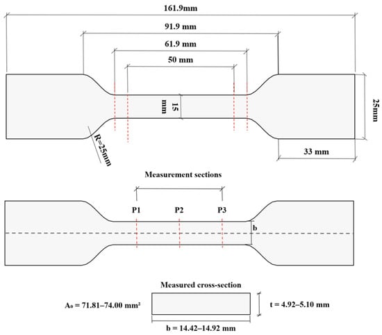
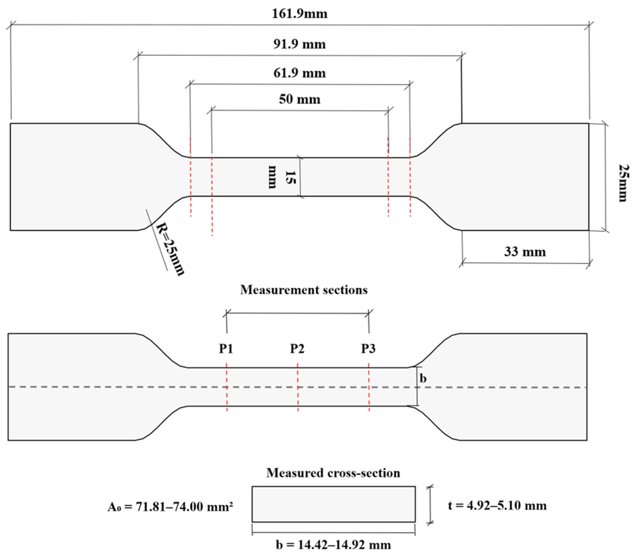
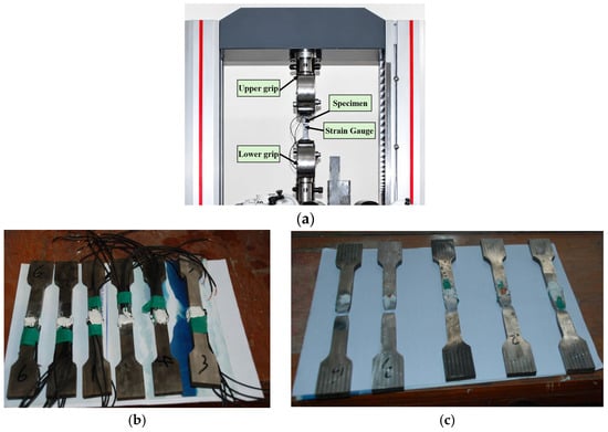
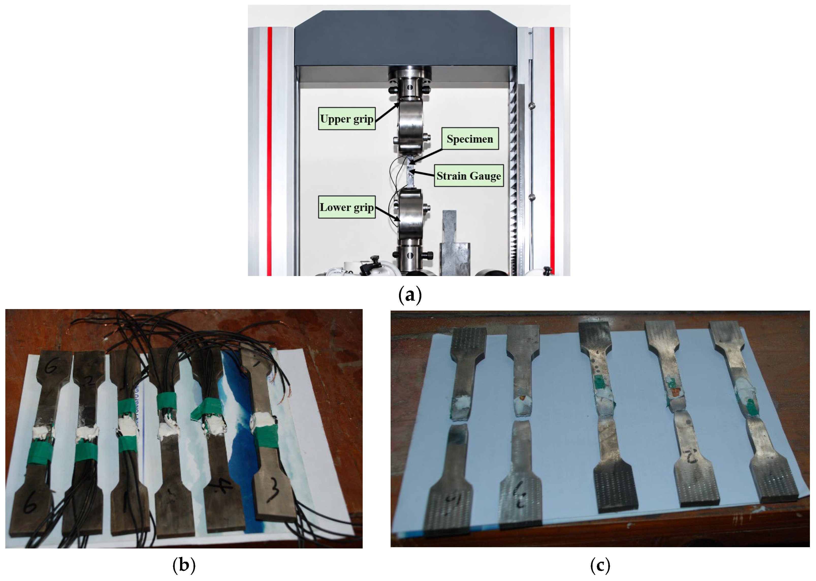
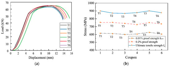
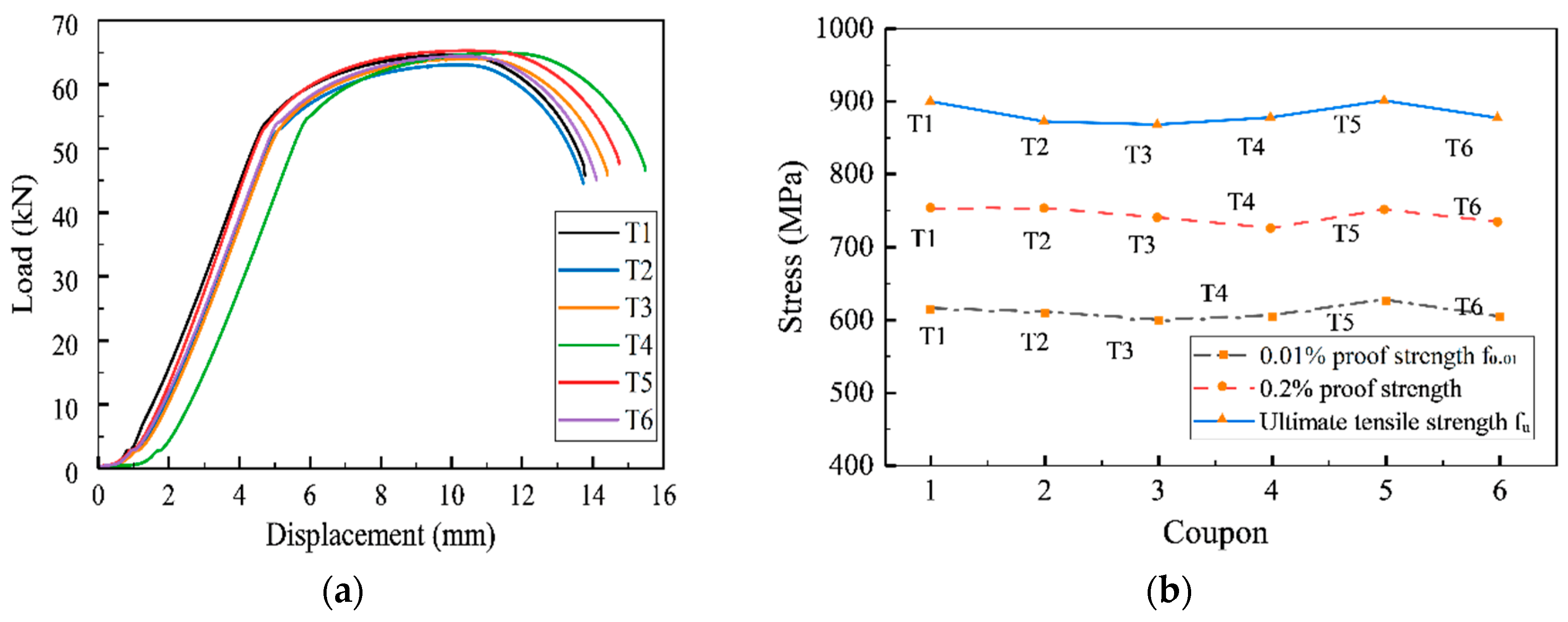
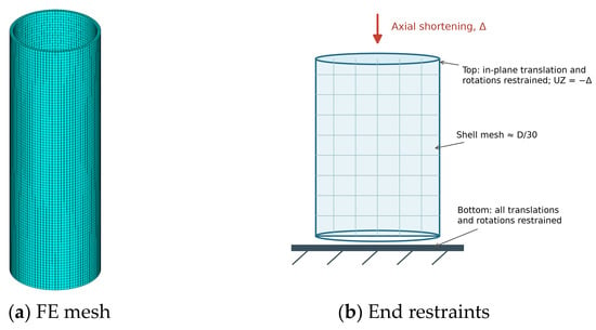
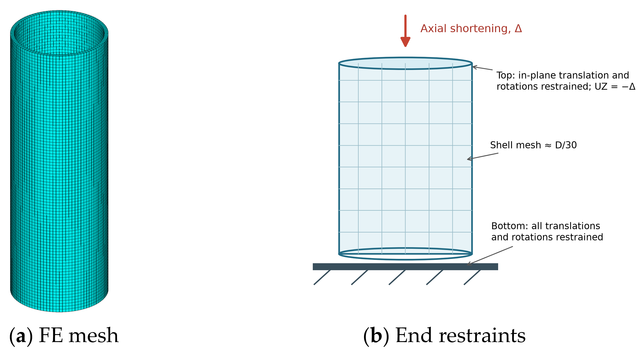
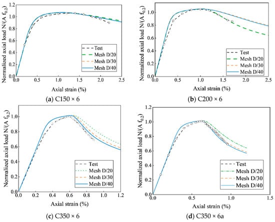
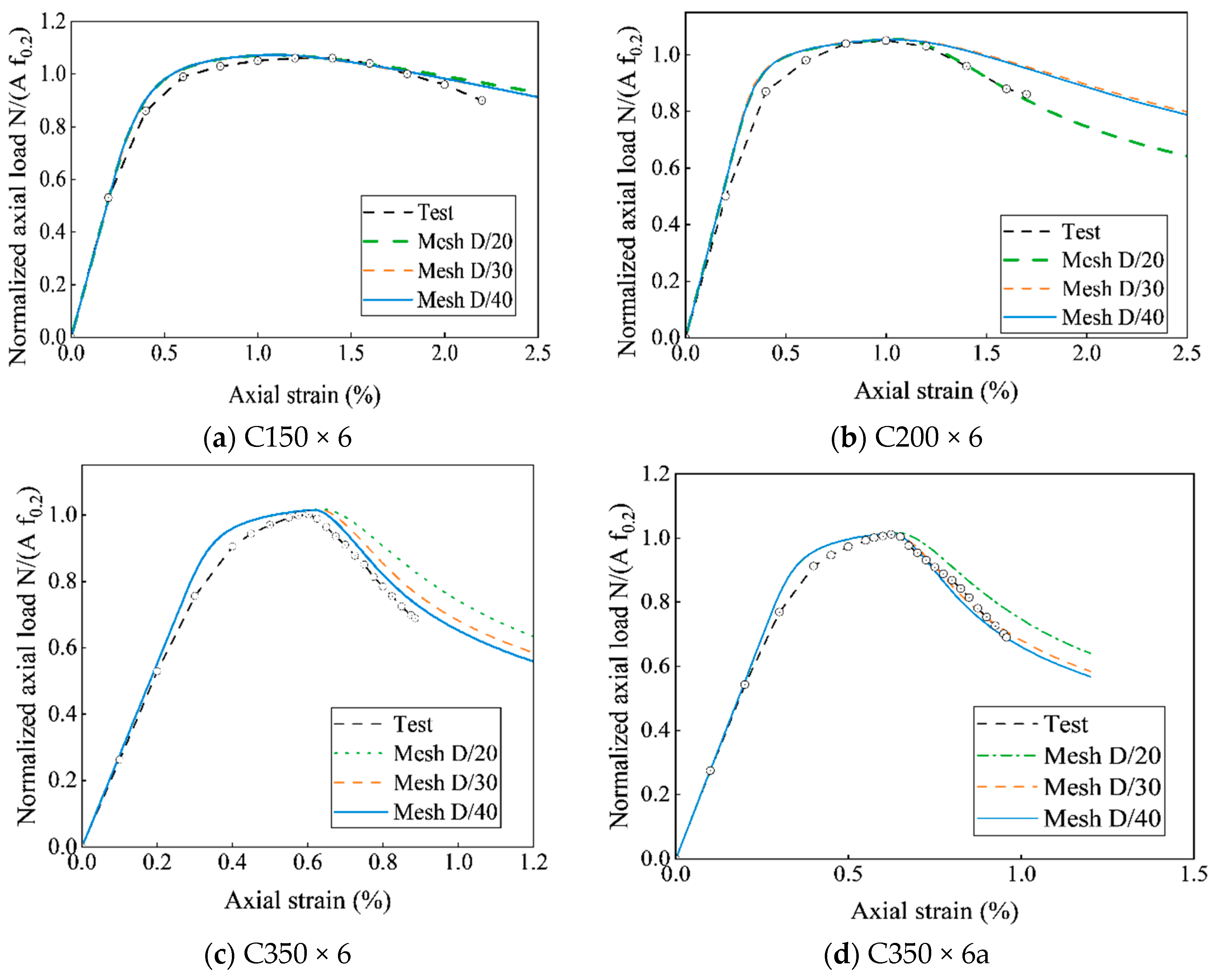
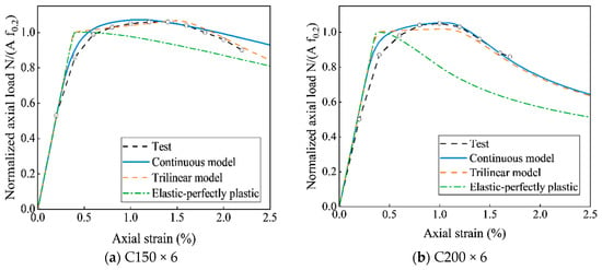
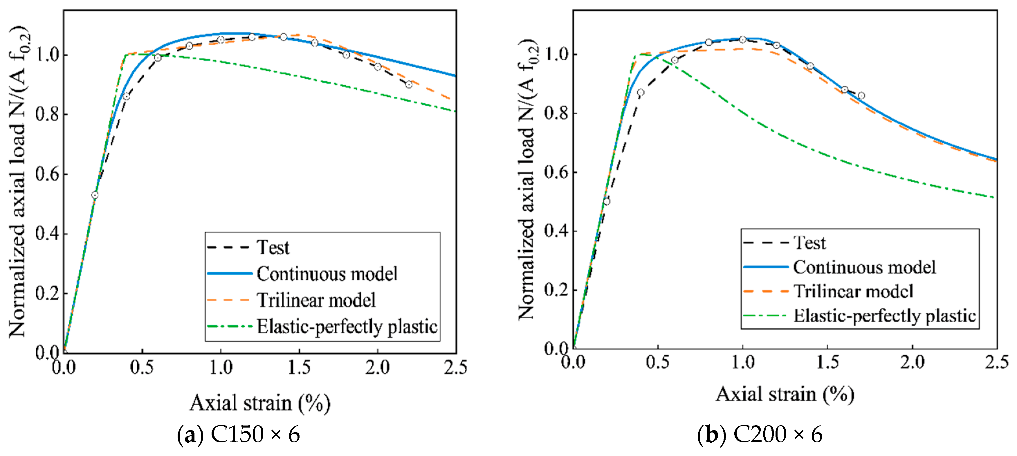
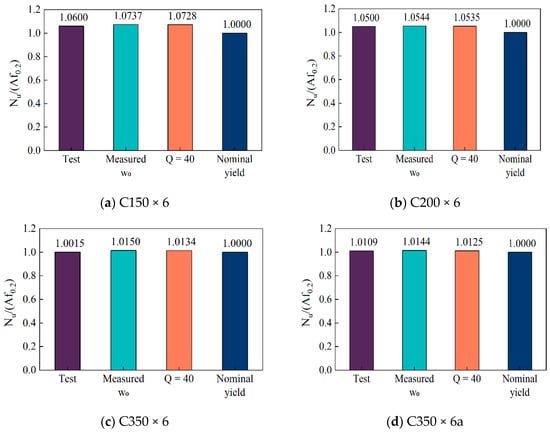
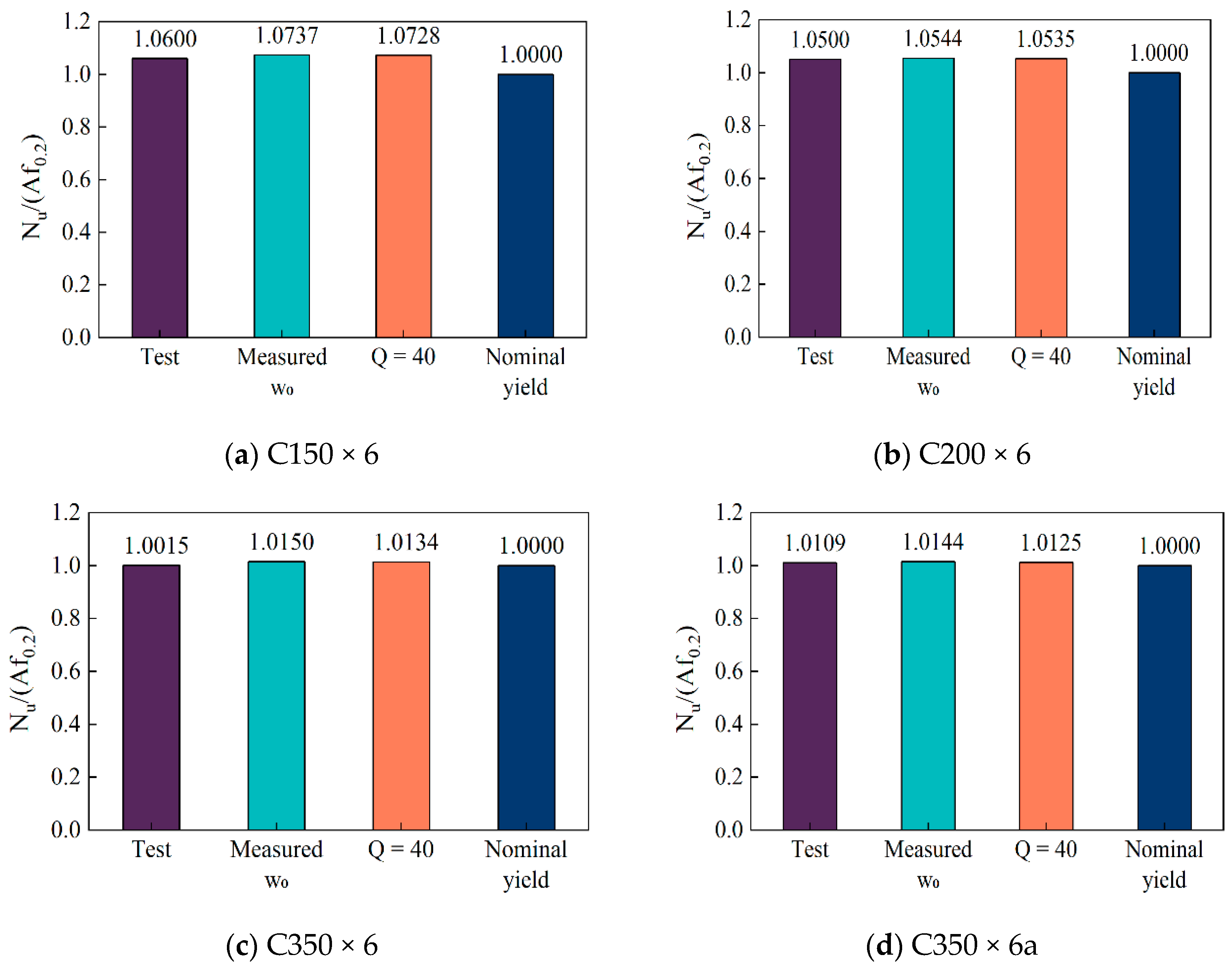
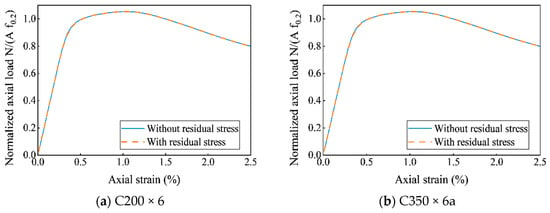
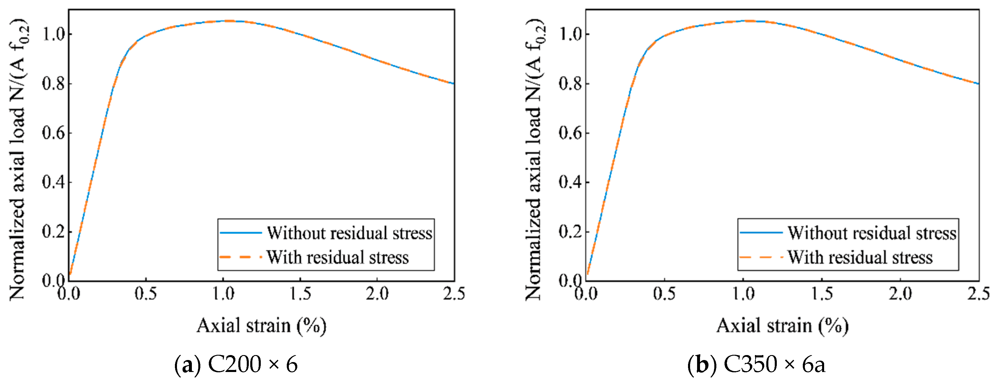
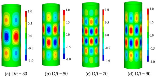
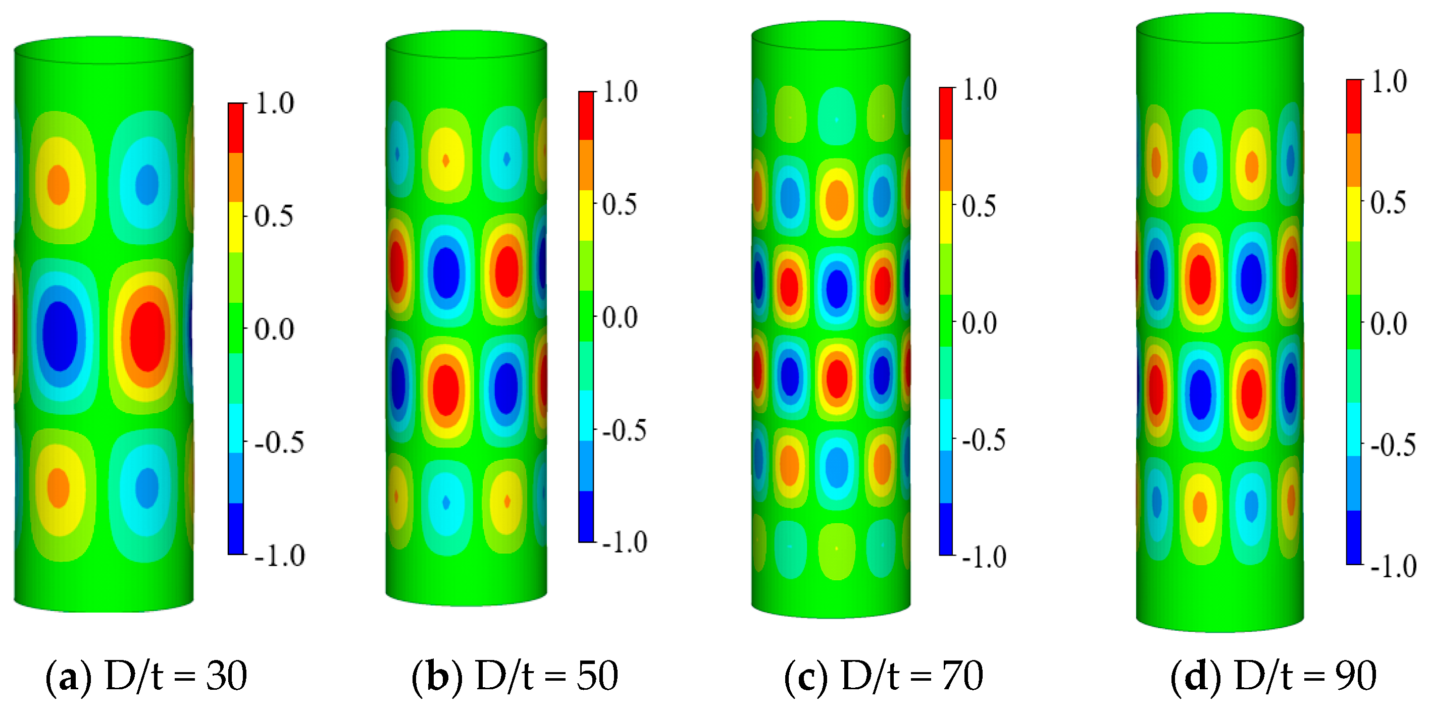
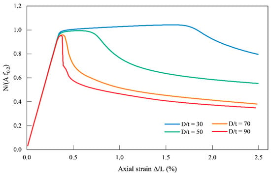
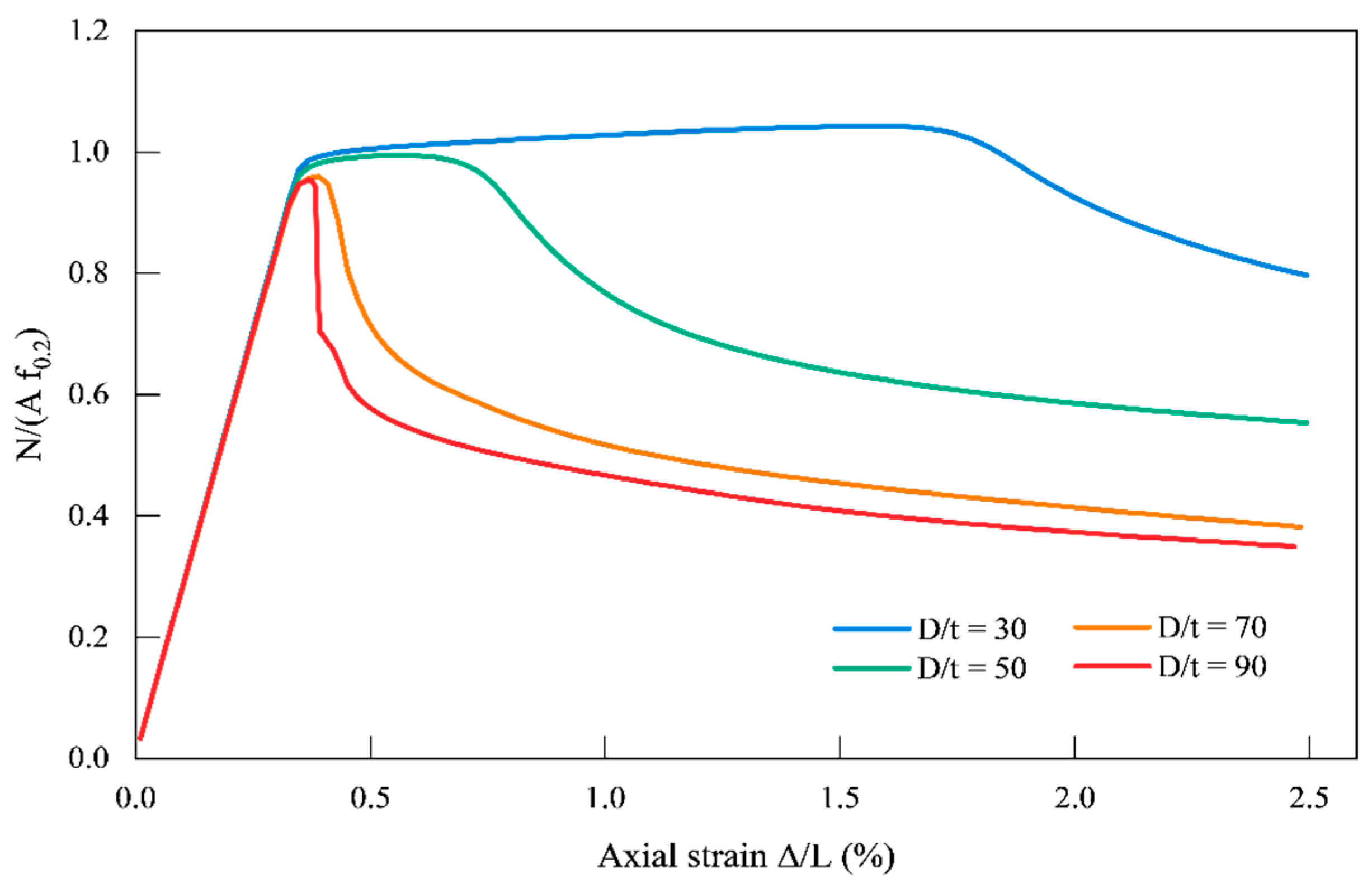
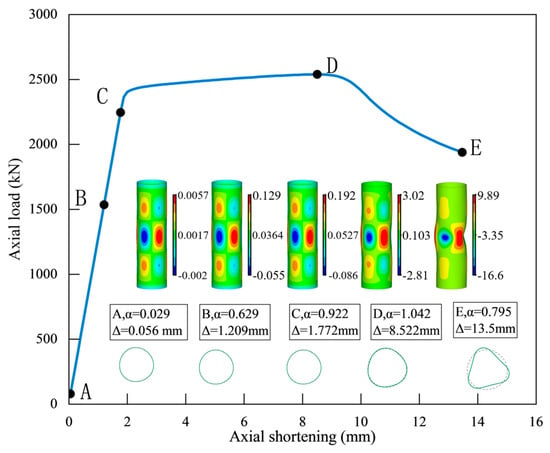
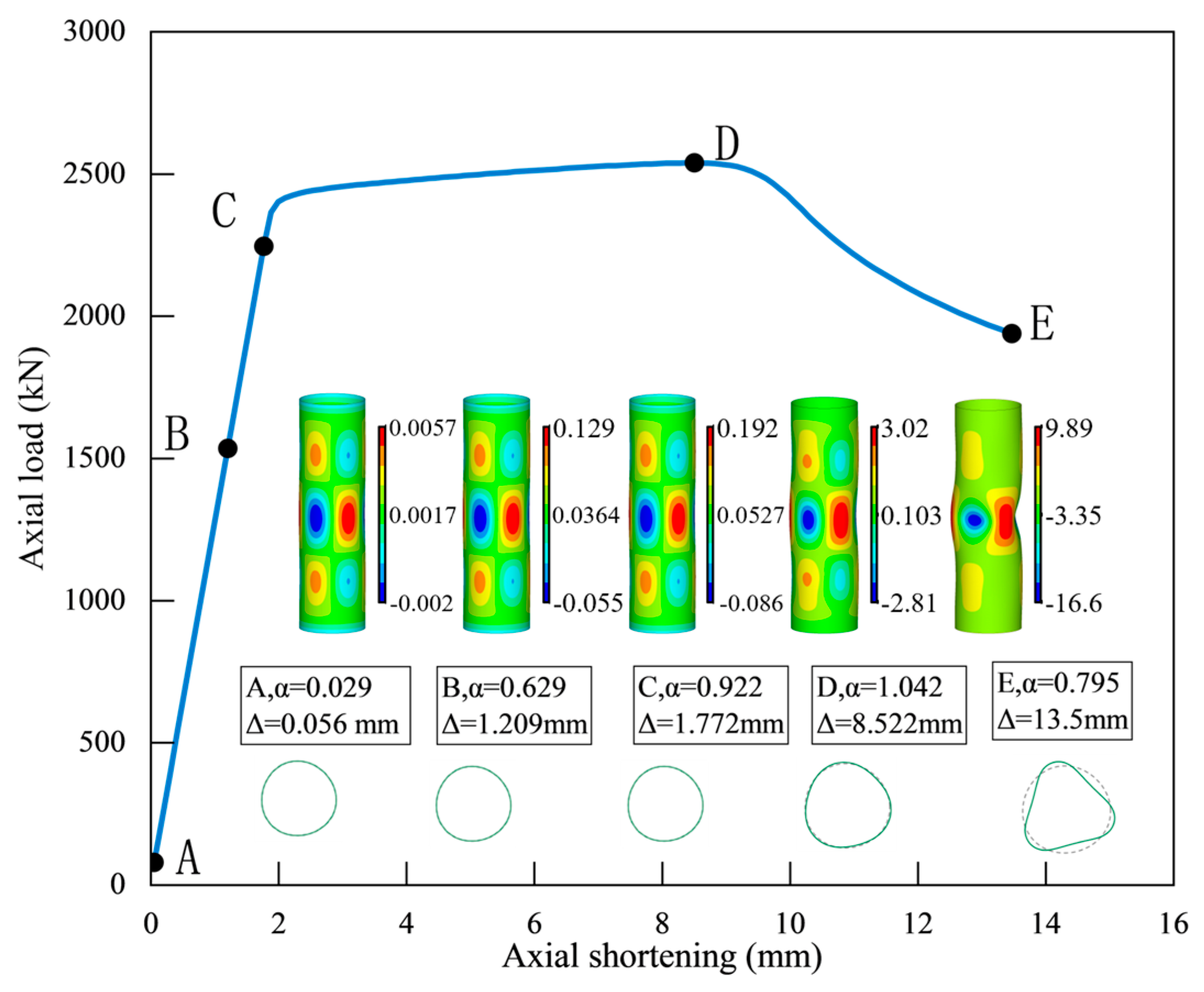
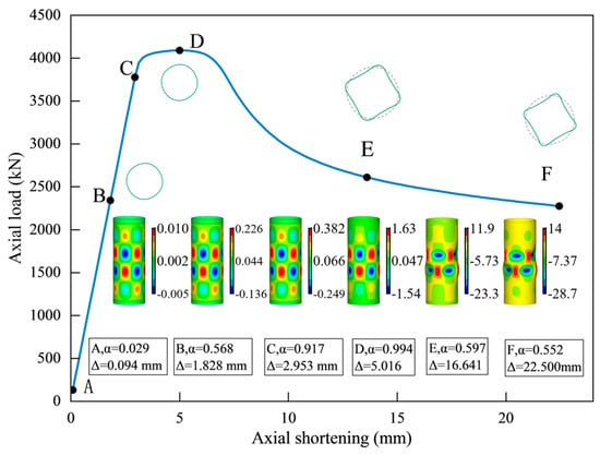
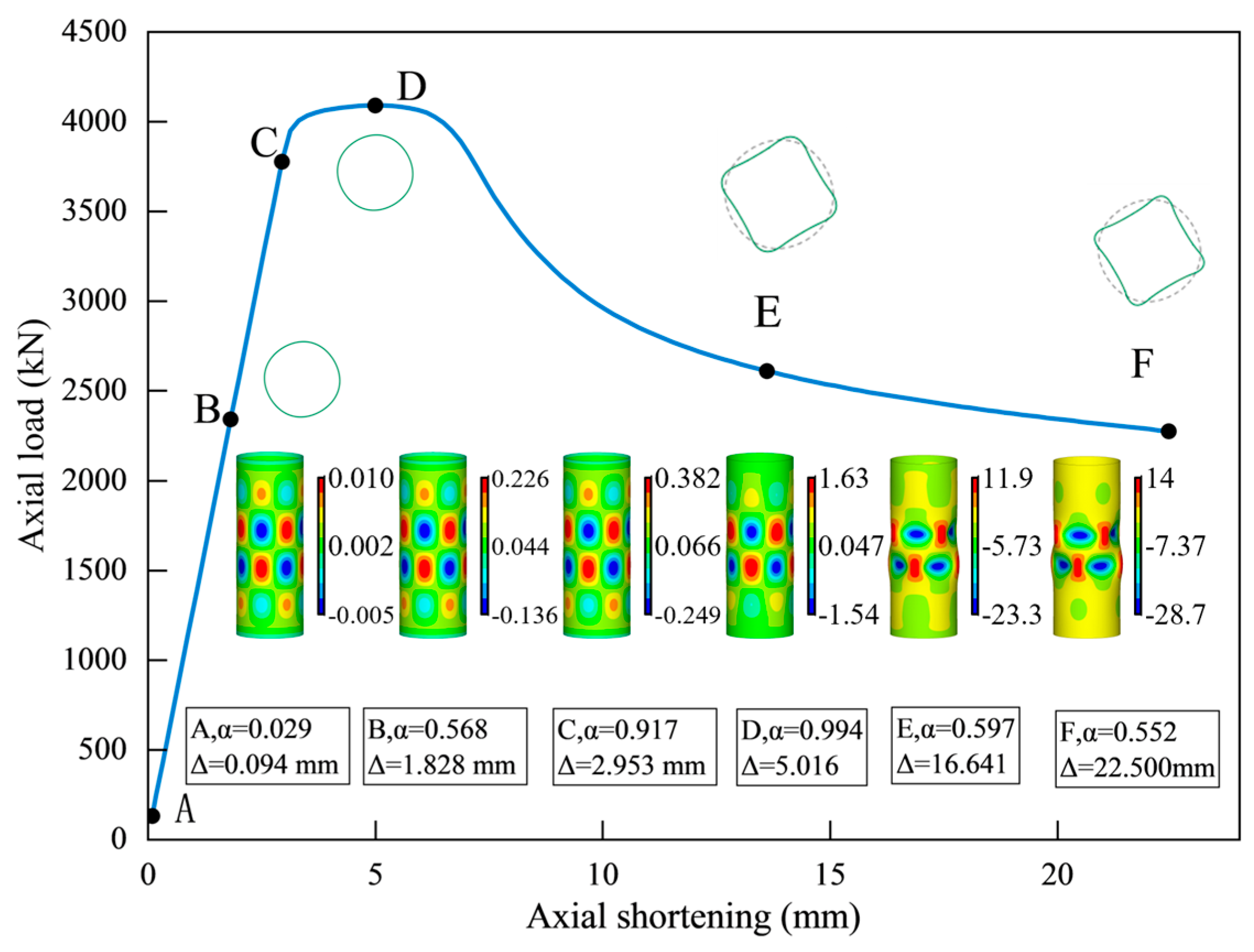
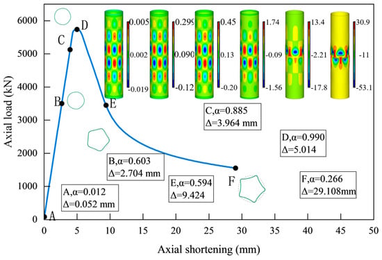
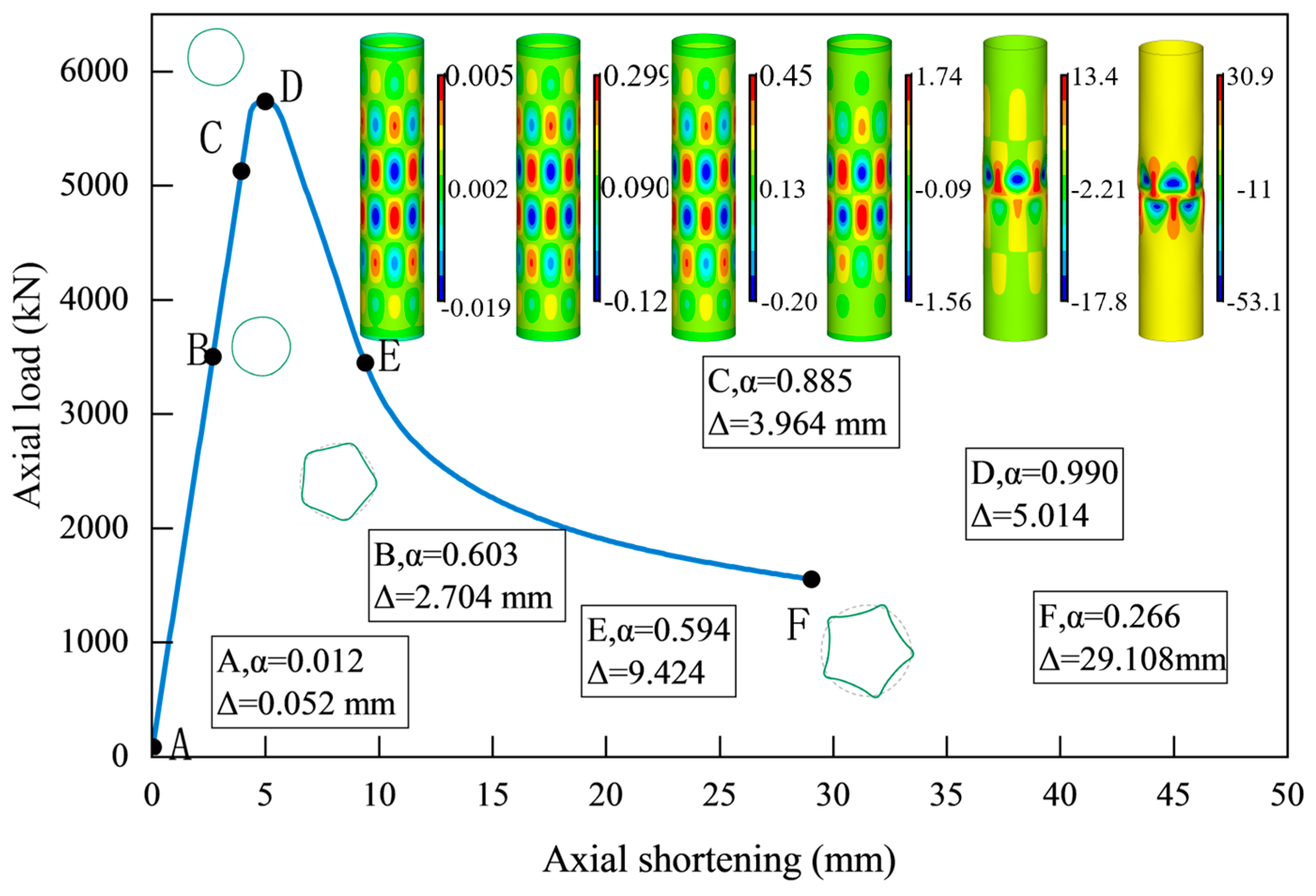
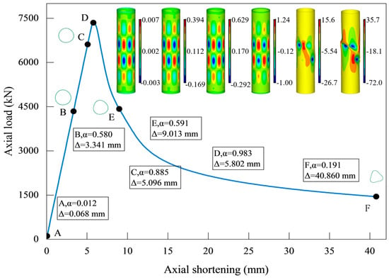
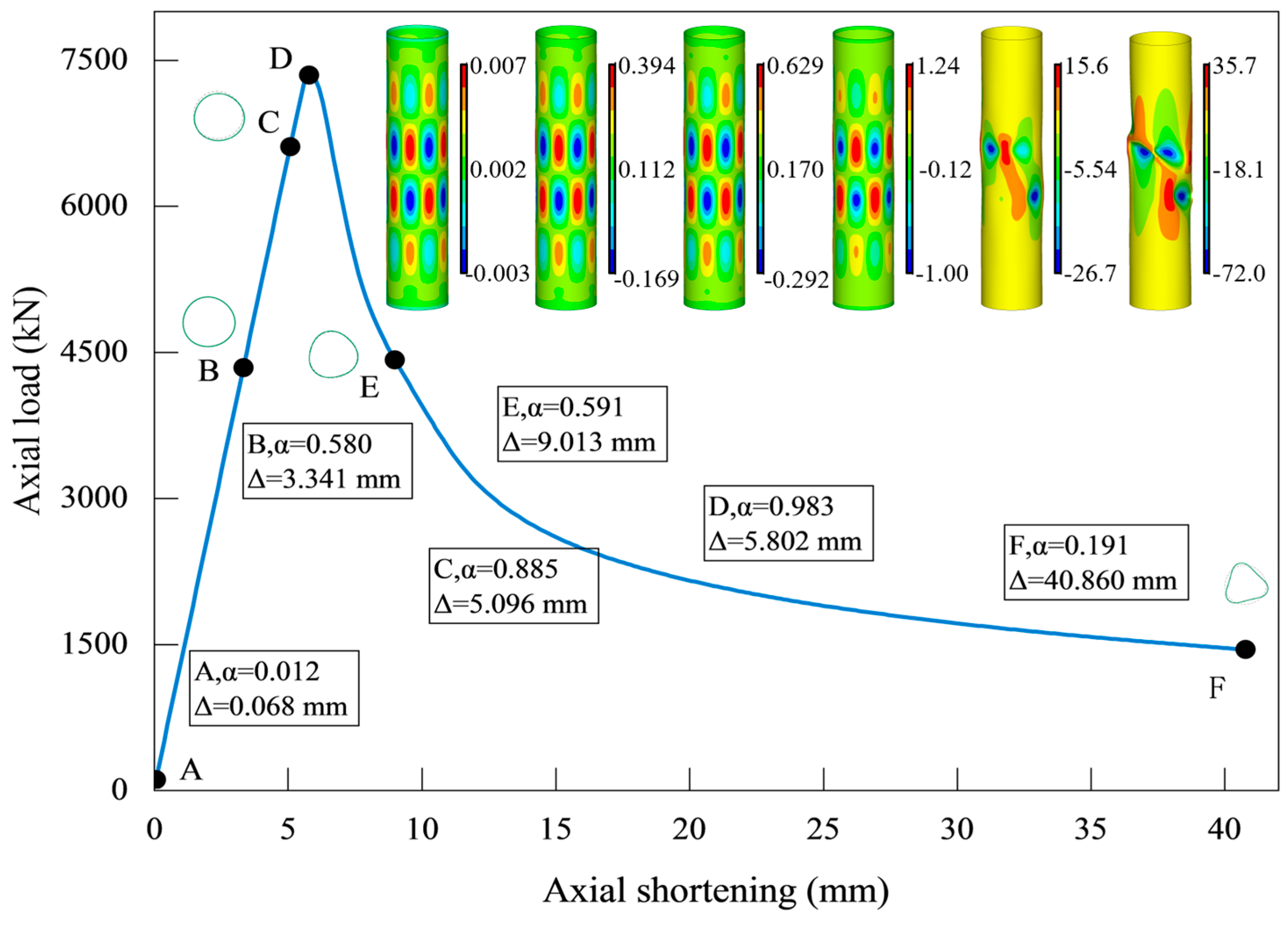
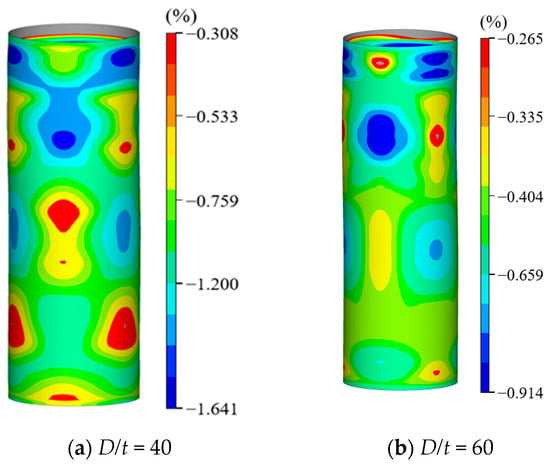
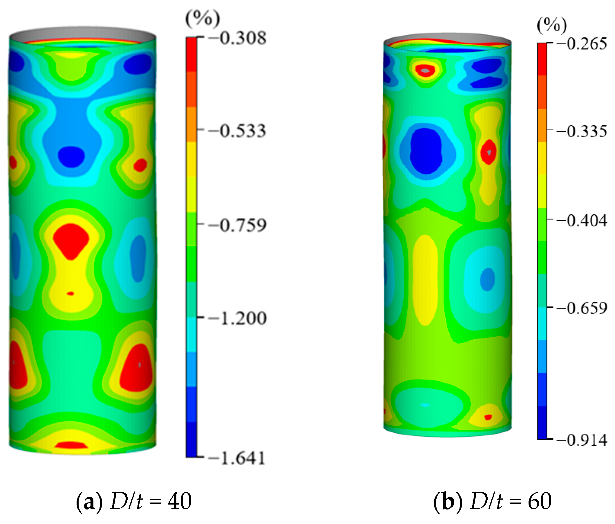
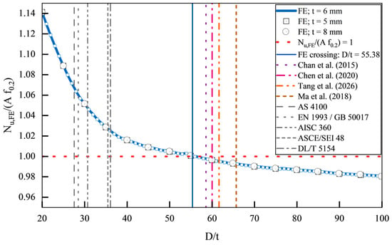
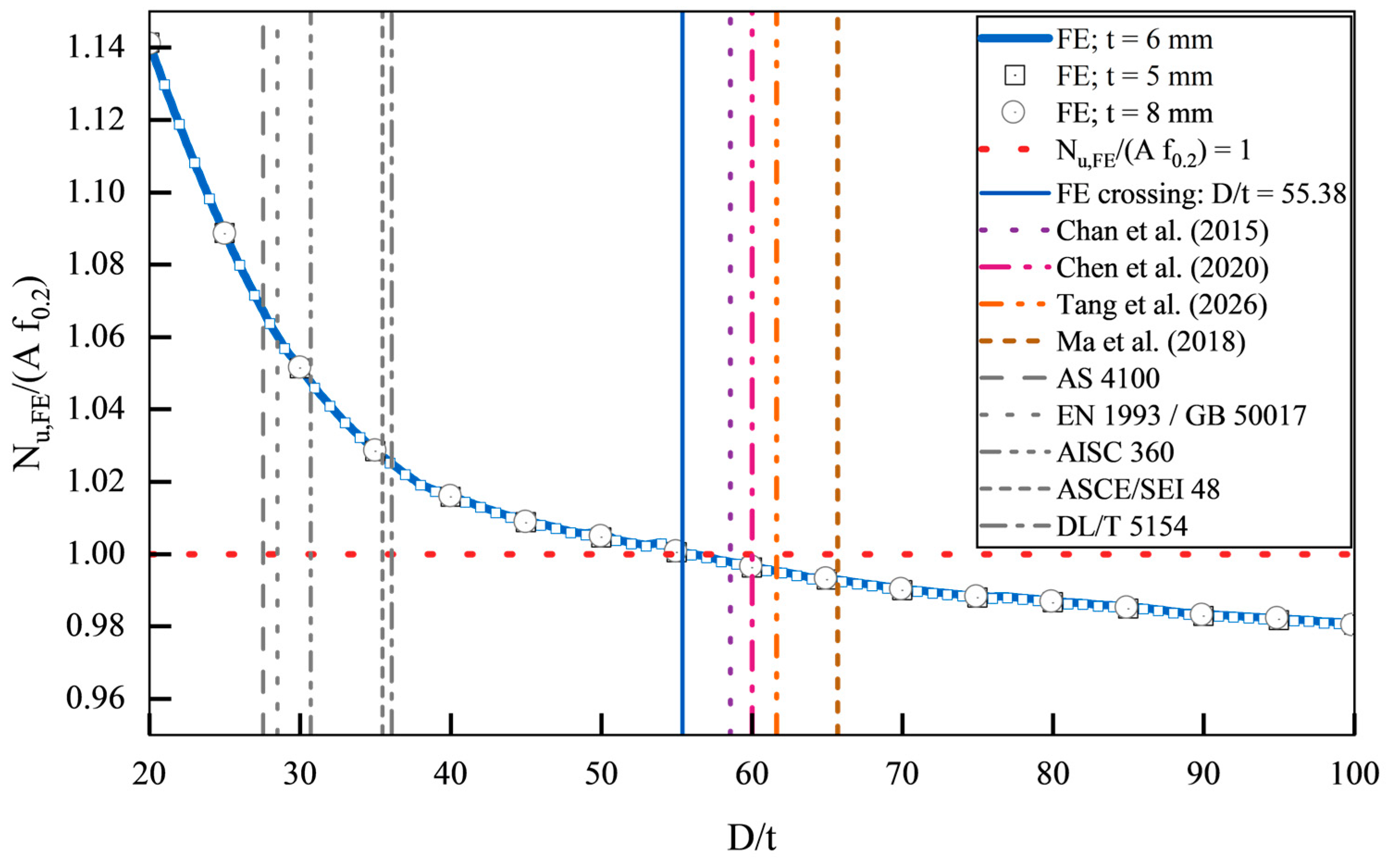
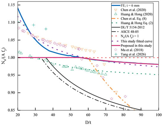
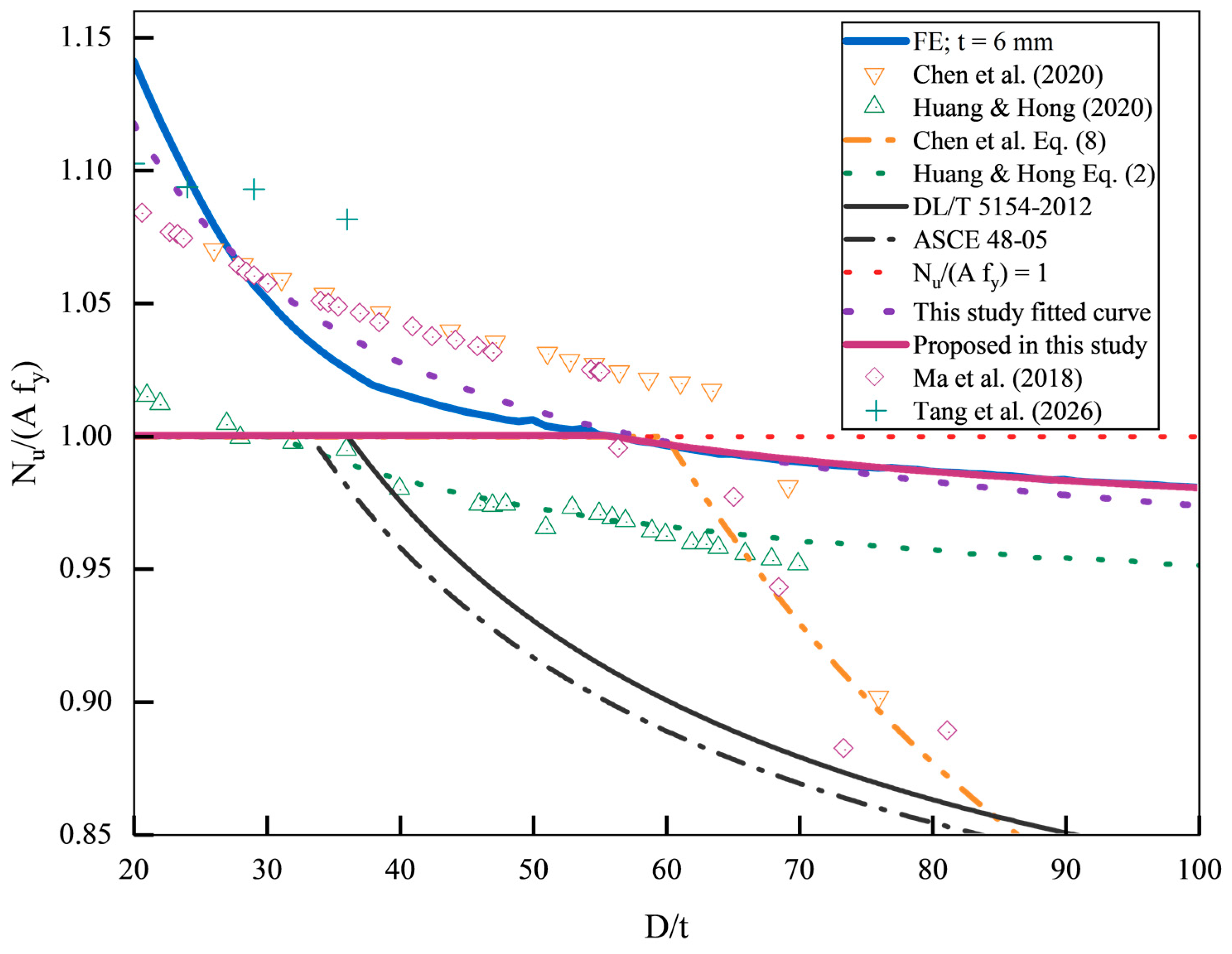
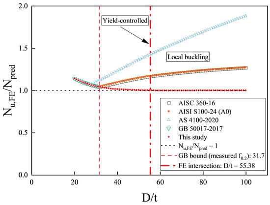
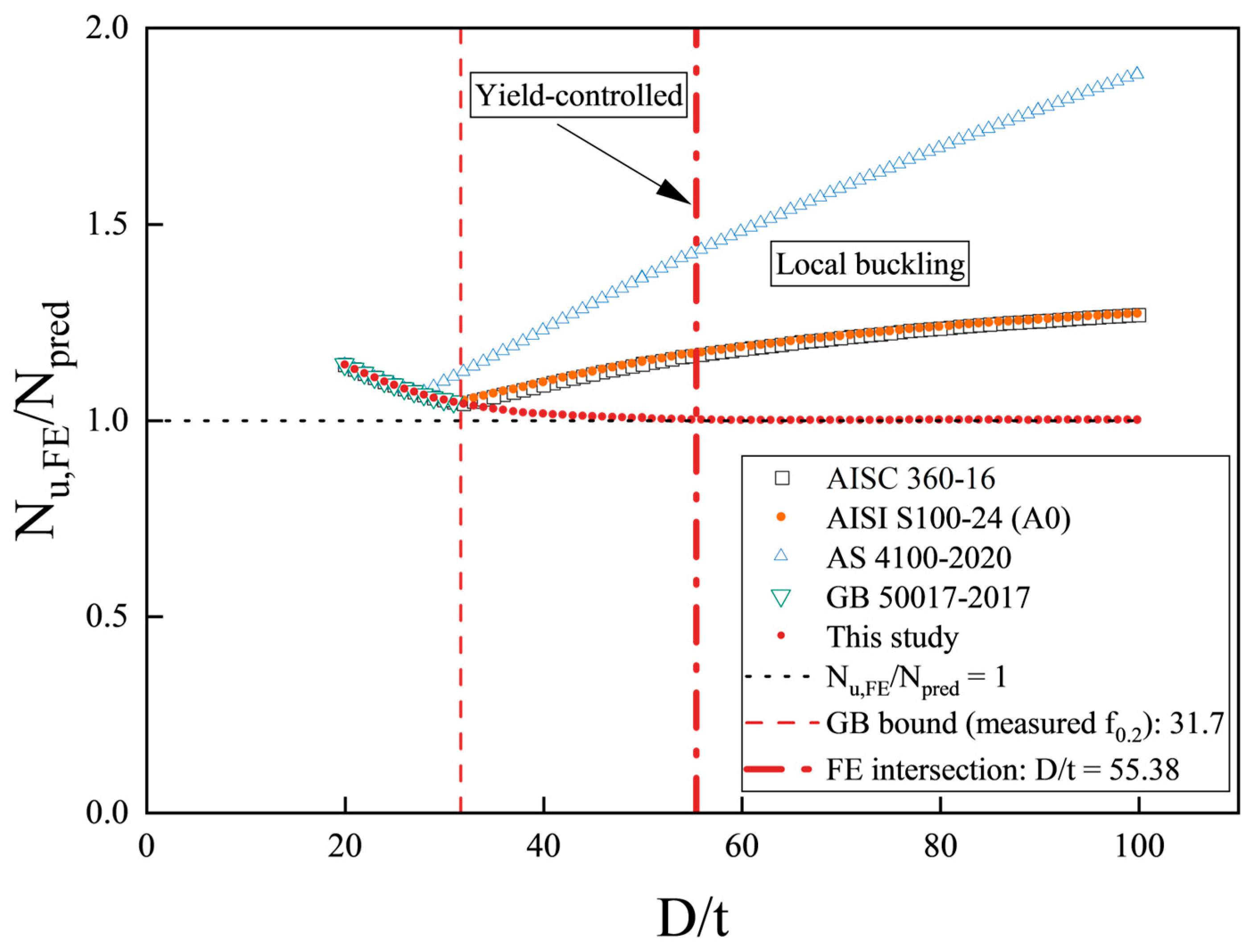
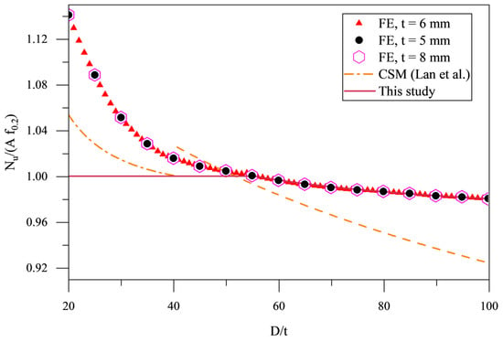
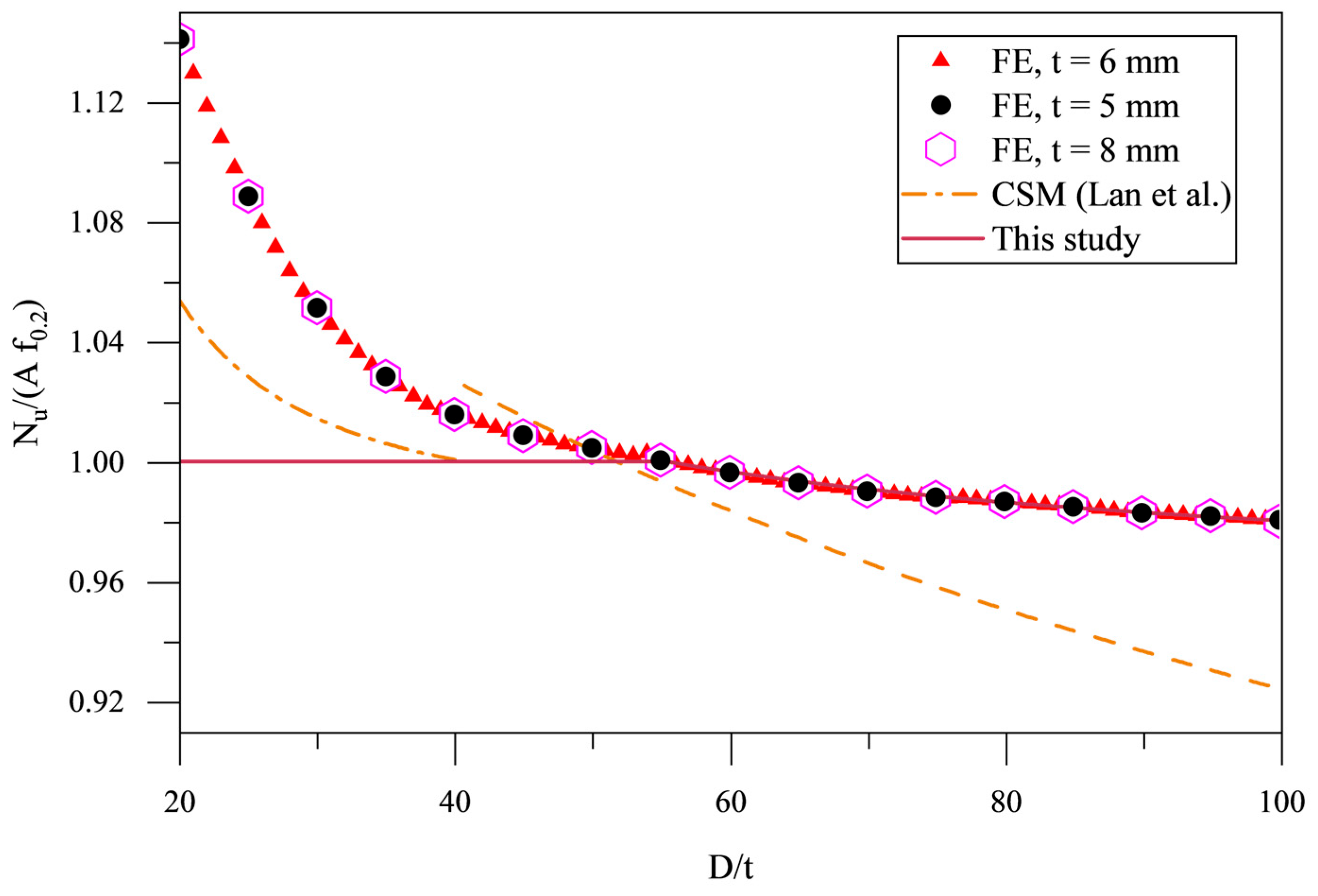

Disclaimer/Publisher’s Note: The statements, opinions and data contained in all publications are solely those of the individual author(s) and contributor(s) and not of MDPI and/or the editor(s). MDPI and/or the editor(s) disclaim responsibility for any injury to people or property resulting from any ideas, methods, instructions or products referred to in the content. |
© 2026 by the authors. Licensee MDPI, Basel, Switzerland. This article is an open access article distributed under the terms and conditions of the Creative Commons Attribution (CC BY) license.