Peridynamic Simulation Method for Excavation Damage of Surrounding Rock in Water-Rich Fractured Strata Tunnels

Abstract

Groundwater seepage and engineering excavation are among the primary causes of rock mass strength degradation and damage failure during tunnel construction. In natural strata, the groundwater seepage field and the rock stress field exist in a state of natural equilibrium. Tunnel excavation disrupts this equilibrium, inducing sudden changes in the original groundwater recharge–migration–discharge system. This may trigger shear slip along internal structural planes and the initiation and propagation of hydraulic fractures, exacerbating the damage and failure of the surrounding rock, and eventually leading to surrounding rock instability or water inrush disasters. Peridynamics (PD) can simulate the damage and failure behavior of rock masses under in situ stress and can also characterize the seepage of groundwater in porous–fractured media. This paper integrates peridynamics for discontinuous deformation and failure of solid materials with groundwater seepage modeling. Based on the effective stress principle, a simulation method is developed for the damage and failure of water-rich fractured rock masses under fluid pressure-driven conditions, in which the conductivity of each fluid bond is controlled by the state of the corresponding solid bond. Furthermore, the material point dormancy method (MPDM), which represents the unloading effect of tunnel excavation, is extended to the fluid field, so that excavation unloading and a drained tunnel surface are treated within one framework. The propagation of hydraulic fractures is simulated for different natural fracture dip angles and stress states and for a random fracture network, and the results are compared with RFPA simulations computed by the authors (a code-to-code consistency check). Tunnel excavation in water-rich jointed strata is then simulated for different joint counts and seepage pressures, and the resulting excavation damage zones and pore water pressure distributions are analyzed. The results are limited to the two-dimensional, homogeneous-matrix cases examined and have not been validated against experimental or field data; they provide a numerical reference for the analysis of excavation-induced damage in surrounding rock of tunnels situated in water-rich fractured strata.

1. Introduction

During the construction and operation of underground engineering works such as tunnels, groundwater seepage and excavation unloading are among the primary causes of rock mass strength weakening and damage failure [1,2]. In natural strata, the groundwater seepage field and the rock stress field exist in a state of natural equilibrium. Engineering excavation disturbance breaks this equilibrium, promotes groundwater circulation, causes shear slip along internal structural planes in the rock mass, and initiates and propagates hydraulic fractures, which may eventually induce major geological disasters such as water inrush [3,4]. A scientific understanding of the mechanisms of rock mass damage and failure induced by groundwater seepage and excavation unloading in fractured rock masses is the theoretical basis for ensuring tunnel construction safety, reducing water inrush disaster risks, and protecting groundwater resources.

Natural rock masses contain numerous discontinuous structural planes such as joints and fractures. The attitude, density, aperture, roughness, and filling state of these fractures significantly influence the rock mass permeability, resulting in pronounced heterogeneity and anisotropy of seepage in fractured rock masses [5,6,7]. Currently, numerical models describing the seepage characteristics of fractured rock masses mainly fall into three categories: equivalent continuum models based on the representative elementary volume (REV) [8], discrete fracture network (DFN) models based on fracture seepage [9,10,11], and dual-porosity media models based on pore–fracture seepage [12,13]. The equivalent continuum model offers high computational efficiency and is suitable for describing the overall seepage behavior of large-scale rock masses; the discrete fracture network model can more realistically reflect the heterogeneity and anisotropy of fracture seepage; and the dual-porosity media model accounts for the seepage characteristics of both porous and fractured media, better matching actual geological conditions. However, within the framework of traditional numerical methods (finite element, finite difference, etc.), all the above models face challenges such as complex fracture geometry description and difficulties in mesh generation [14,15].

Peridynamics (PD) is a nonlocal continuum mechanics theory proposed by Silling [16] in 2000. Its core idea is to reformulate the partial differential equations of classical continuum mechanics into integral equations, thereby naturally avoiding the singularity difficulties that classical theory encounters when dealing with discontinuity problems. A meshfree discretization of the theory, which is the basis of the numerical implementation used in this paper, was introduced by Silling and Askari [17]. Peridynamic theory has been successfully applied to fields such as crack propagation in solid materials [18,19] and rock failure [20,21]. In recent years, researchers have extended the nonlocal interaction concept of peridynamics to transport problems including heat conduction [22] and flow in porous media [23,24]. Katiyar et al. [24] first established the peridynamic governing equations for seepage in porous media and derived the relationship between microscopic permeability and macroscopic permeability; Nadimi et al. [25] simulated hydraulic fracturing with peridynamics in a heterogeneous medium, and Oterkus et al. [26] proposed a poroelastic peridynamic formulation for fluid-filled fractures; Ouchi et al. [27] further established a peridynamic framework for fluid–solid coupling (see also [28,29]).

Although peridynamics has made progressive advances in the fields of rock mass seepage and fluid–solid coupling, several key bottlenecks remain to be resolved in peridynamic fluid–solid coupling models for fractured rock masses compared to its mature applications in solid fracture and crack propagation. First, existing peridynamic seepage models mainly focus on homogeneous porous media or simple fracture characterization, and a systematic theoretical foundation is still lacking for characterizing the non-uniform seepage features of pore–fracture dual-porosity media. Second, the coupling mechanisms among the seepage field, stress field, and damage field in fractured rock masses is extremely complex; existing coupling models mostly emphasize single-field or dual-field coupling, making it difficult to fully characterize the synergistic effect of hydraulic fracture initiation–propagation and rock mass damage evolution, especially lacking analysis of the influence of natural fracture occurrence on the coupling process. Third, excavation unloading causes stress redistribution, and its superposition with groundwater seepage is key to inducing damage and failure in tunnel surrounding rock. However, a peridynamic simulation method that couples excavation unloading with groundwater seepage in fractured rock masses has not yet been developed, which restricts its application in actual tunnel engineering.

Existing peridynamic studies have addressed flow in porous media, hydromechanical coupling with fracturing, and the excavation of dry rock using the material point dormancy method (MPDM). The contributions of this paper are as follows. (a) A pore–fracture flow model in which the conductivity of each fluid bond is controlled by the state of the corresponding solid bond (crossing a pre-existing joint, or bond breakage), so that newly formed fractures create high-conductance paths without a predefined fracture geometry. (b) A coupling of flow and mechanics through the effective stress with the Biot coefficient, including the fluid pressure acting on broken bonds. (c) The extension of MPDM from the solid bonds to the fluid field, so that excavation unloading and the drained tunnel surface are treated consistently within one framework.

Based on the nonlocal interaction concept of peridynamics, this paper establishes a peridynamic model for pore–fracture dual-porosity media seepage. On this basis, a simulation method for stress–seepage coupling in fractured rock masses is constructed based on the effective stress principle. Furthermore, the material point dormancy method is introduced to establish a peridynamic simulation method for damage and failure of fractured rock masses under coupled unloading and seepage effects. The consistency of the model and method with RFPA results computed by the authors is examined, and the influence of hydraulic fracturing in natural fractured rock masses and groundwater seepage on the excavation damage zone of tunnels is analyzed, providing a numerical approach for simulating excavation damage in surrounding rock of tunnels in water-rich fractured strata.

2. Stress–Seepage Simulation Method for Fractured Rock Masses

2.1. Pore–Fracture Dual-Porosity Media Seepage Model

The pore–fracture dual-porosity media seepage model treats the voids in the rock mass as a dual structure composed of pores and fractures: in addition to seepage through the fracture network, the rock matrix is assumed to be an equivalent continuum with a relatively small permeability coefficient. In the present peridynamic implementation, a single pore pressure is stored at each material point, and the pore and fracture systems are distinguished only by the conductivity of the fluid bonds. The model is therefore a single-pressure (equivalent) dual-porosity model: it differs from the classical Barenblatt–Warren–Root models [12,13], which carry two pressure fields coupled by an explicit inter-porosity exchange term.

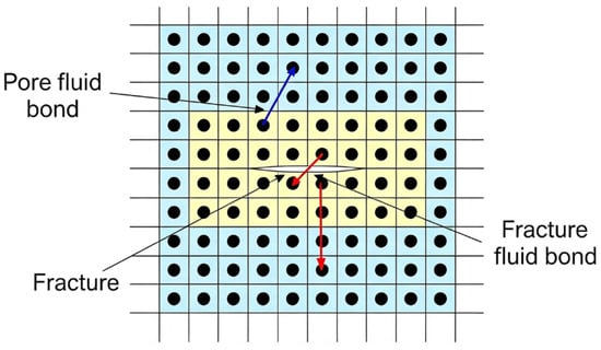
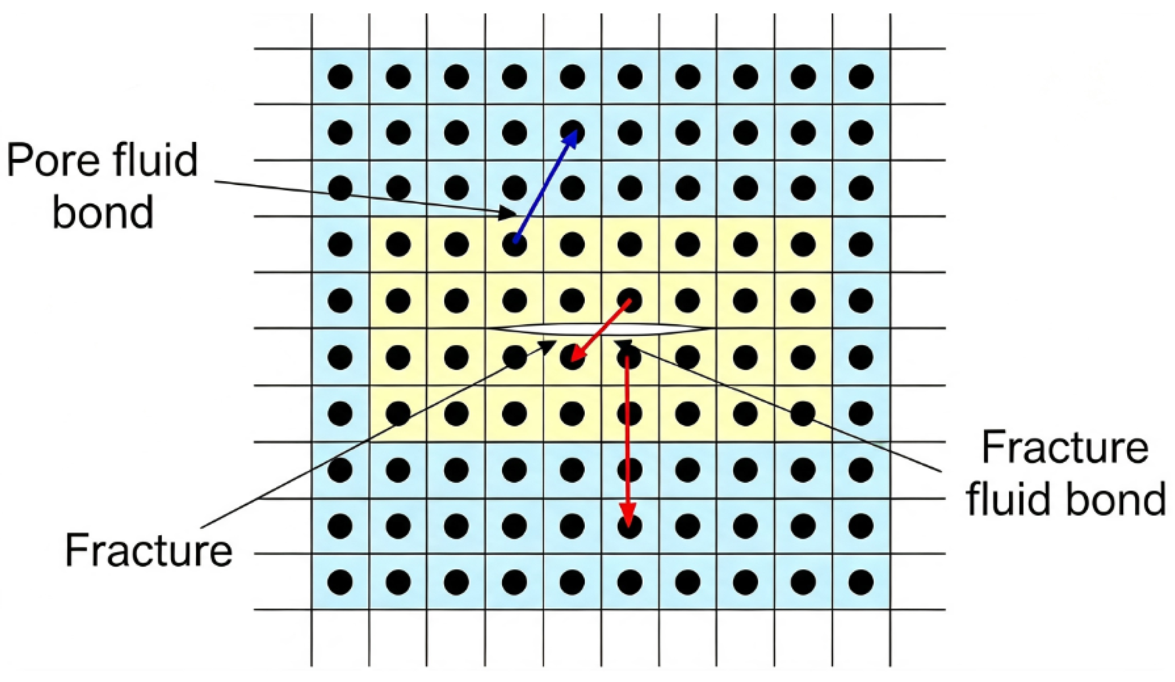
Based on the nonlocal interaction concept of peridynamics, a pore–fracture dual-porosity media seepage model is established by dividing fluid bonds into pore fluid bonds and fracture fluid bonds, and considering the flow exchange between them through the bond fluxes, as shown in Figure 1. Material points within a certain range of the fracture surface are considered to possess fracture seepage characteristics in the rock mass. This is because solid bonds crossing the fracture surface are broken (or, for pre-existing joints in Section 4.2 and Section 5, weakened), and the fluid bonds exhibit fracture flow characteristics (fracture fluid bonds); in other areas without fractures, the solid bonds are intact, and the fluid bonds exhibit pore flow characteristics (pore fluid bonds).

Figure 1. Schematic diagram of peridynamic pore–fracture dual-media seepage model.

By combining the basic equations for seepage in porous media and those for seepage in fractured media, and based on the integrity and seepage characteristics of material point bonds, the basic equations for pore–fracture dual-porosity media seepage can be obtained.

Pore fluid bond:

$${\displaystyle \frac{\partial }{\partial t}}\left(\rho \left[{\mathbf{x}}_i\right]\phi \left[{\mathbf{x}}_i\right]\right)={\int }_{H_x}{\displaystyle \frac{\rho \left[{\mathbf{x}}_i,{\mathbf{x}}_j\right]}{\mu }}{\displaystyle \frac{4k}{\pi {\delta }^2}}{\displaystyle \frac{\Phi \left[{\mathbf{x}}_j\right]-\Phi \left[{\mathbf{x}}_i\right]}{{∥{\mathit{\xi }}_{{\mathbf{x}}_i{\mathbf{x}}_j}∥}^2}}\mathrm{d}{A}_{{\mathbf{x}}_j}+R\left[{\mathbf{x}}_i\right]$$

(1)

where $\Phi$ is the hydraulic potential at any material point, $\mu$ is the fluid viscosity, k is the permeability of the pore fluid bond, $\rho$ is the fluid density, $\phi$ is the porosity of the pore fluid bond, $\delta$ is the neighborhood size of the material point, $\mathrm{d}A$ is the area element of the material point ${\mathbf{x}}_j$, R is the source/sink term of the pore fluid bond, $\mathit{\xi }$ is the relative position between material points ${\mathbf{x}}_i$ and ${\mathbf{x}}_j$, and $H_x$ is the neighborhood range of the material point.

Fracture fluid bond:

$${\displaystyle \frac{\partial }{\partial t}}\left(\rho \left[{\mathbf{x}}_i\right]{\phi }_{\mathrm{f}}\left[{\mathbf{x}}_i\right]\right)={\int }_{H_x}{\displaystyle \frac{\rho \left[{\mathbf{x}}_i,{\mathbf{x}}_j\right]}{\mu }}{\displaystyle \frac{4k_{\mathrm{f}}}{\pi {\delta }^2}}{\displaystyle \frac{\Phi \left[{\mathbf{x}}_j\right]-\Phi \left[{\mathbf{x}}_i\right]}{{∥{\mathit{\xi }}_{{\mathbf{x}}_i{\mathbf{x}}_j}∥}^2}}\mathrm{d}{A}_{{\mathbf{x}}_j}+R_{\mathrm{f}}\left[{\mathbf{x}}_i\right]$$

(2)

where ${\phi }_{\mathrm{f}}$ is the porosity of the fracture fluid bond, $k_{\mathrm{f}}$ is the permeability of the fracture fluid bond, and $R_{\mathrm{f}}$ is the source/sink term of the fracture fluid bond.

Bond Classification, Conductivity and Exchange

In the numerical implementation, a single pore pressure p is stored at each material point, so that the pore and fracture systems share one pressure field and the exchange between them takes place through the bond fluxes. The equations are integrated explicitly in pressure form, using the fluid compressibility $c_w$; the flux coefficient of a bond is $2k/\left(\pi \delta \phi \mu c_w\right|\mathit{\xi }{|}^3)$, so that the pressure evolution depends on the permeability, porosity, viscosity and compressibility only through this combination. This corresponds to a kernel $1/{|\mathit{\xi }|}^3$ with the normalization $2/\left(\pi \delta \right)$ in two dimensions, which, like the kernel $1/{|\mathit{\xi }|}^2$ with the normalization $4/\left(\pi {\delta }^2\right)$ written in Equations (1) and (2), reproduces the classical operator $(k/\mu ){\nabla }^{2}p$ in the local limit. Conductivity is assigned bond by bond.

A fluid bond is classified as a fracture bond if (i) it crosses a pre-existing fracture or joint, or (ii) its solid bond has broken, i.e., its stretch exceeds the critical stretch $s_0$. All other bonds are pore bonds. The classification is irreversible. It is used as a proxy for a connected opening along the bond direction: newly formed fractures thus create new high-conductance paths, and the connectivity of the high-conductance network grows with the network of broken bonds, without a predefined fracture geometry. The conductivity of a fracture bond is a lumped effective value (it is not an aperture-based cubic-law value) and does not depend on stress or opening. Because the classification is made per bond, no averaging rule is needed for bonds connecting points of different types. The bond flux is antisymmetric, so that the exchange between two material points is balanced. The pressure field is updated in place in each fluid sub-step; mass conservation is therefore approximate (see Appendix A for an error estimate). The terms R and $R_f$ represent external sources and sinks. In the implementation they are realized as prescribed-pressure conditions: the injection zone (Section 4.1 and Section 4.2), the virtual boundary layers with zero pressure (Section 4.1 and Section 4.2), the top and bottom boundaries with prescribed pressure (Section 5), and the excavated points with zero pressure (Section 5). No other source term and no separate pore–fracture exchange term are used; the interaction between the pore and fracture systems takes place through the bond fluxes.

In the hydraulic fracturing models of Section 4, the intact bonds are non-conductive (matrix flow is neglected), and only fracture bonds conduct water. In the tunnel models of Section 5, intact bonds have the matrix conductivity, and fracture bonds have a conductivity 1000 times larger. The hydraulic fracturing models of Section 4.1 and Section 4.2 are therefore fracture-dominated limiting cases of the dual-porosity model; the complete dual-porosity model is used in Section 5.

2.2. Stress–Seepage Coupling Simulation Method for Fractured Rock Masses

Affected by geological structures, tunnel surrounding rock exists not only in a certain in situ stress environment but also within a certain seepage field. There is mutual interaction between the stress field and the seepage field, which is referred to as stress–seepage coupling or fluid–solid coupling. The fluid–solid coupling effect in fractured rock masses manifests mainly in two aspects: first, when groundwater seeps through fractured rock masses, it generates seepage forces in the rock mass, mainly including hydrostatic pressure and dynamic water pressure, thereby altering the original stress state of the rock mass; second, changes in the stress state of the fractured rock mass cause deformation or even failure of the rock mass structure, thereby changing the permeability performance and groundwater seepage paths of the fractured rock mass.

The effective stress principle, when applied to analyzing the mechanical properties of saturated soils, has provided an understanding consistent with objective laws and has played a significant role in promoting soil mechanics as an independent discipline. However, because the solid phase of rock materials is continuous rather than granular, the effective stress principle is no longer directly applicable. Therefore, by introducing a correction coefficient that accounts for the volumetric compression deformation of saturated materials, an effective stress expression applicable to rock materials can be established [30]:

$${\sigma }^{\prime }=\sigma -\alpha p$$

(3)

where ${\sigma }^{\prime }$ is the effective stress, $\sigma$ is the total stress, p is the pore water pressure, and $\alpha$ is the Biot coefficient, representing the contribution of pore water pressure to the effective stress, expressed as $\alpha =(1-c_s/c)$, where c is the compressibility of the rock material and $c_s$ is the compressibility of the solid rock phase. In this paper the Biot coefficient is not computed from this expression but is taken directly as a constant, $\alpha =0.8$ (Section 4.2 and Section 5; the same value is used in Section 4.1), which lies within the reasonable range for rock.

Based on the effective stress principle, this paper proposes a peridynamic material point dual-cover theoretical model for simulating fluid–solid coupling in fractured rock masses. In this model, a material point not only possesses solid mechanical properties characterizing material deformation but also acts as a water-storage “container.” Groundwater transmits pore water pressure through bonds between material points. Due to the effect of pore water pressure, the solid bonds of material points are weakened, and they must also withstand the seepage pressure on the fracture surface. In contrast to the state of solid bonds, damage-induced breakage of solid bonds activates fluid bonds, and at this point, broken bonds possess higher permeability.

When considering the coupled groundwater stress–seepage effect, according to the effective stress principle, the interaction force between peridynamic material points is modified as follows:

$${\mathbf{T}}_{\left(i\right)\left(j\right)}\left[{\mathbf{u}}_{\left(j\right)}-{\mathbf{u}}_{\left(i\right)},{\mathbf{x}}_{\left(j\right)}-{\mathbf{x}}_{\left(i\right)},t\right]=\left[{\displaystyle \frac{1}{2}}A-{\displaystyle \frac{2\alpha p_{\left(i\right)}}{mh}}\omega \left|{\mathbf{x}}_{\left(j\right)}-{\mathbf{x}}_{\left(i\right)}\right|\right]{\displaystyle \frac{{\mathbf{y}}_{\left(j\right)}-{\mathbf{y}}_{\left(i\right)}}{\left|{\mathbf{y}}_{\left(j\right)}-{\mathbf{y}}_{\left(i\right)}\right|}}$$

(4)

$${\mathbf{T}}_{\left(j\right)\left(i\right)}\left[{\mathbf{u}}_{\left(i\right)}-{\mathbf{u}}_{\left(j\right)},{\mathbf{x}}_{\left(i\right)}-{\mathbf{x}}_{\left(j\right)},t\right]=\left[{\displaystyle \frac{1}{2}}B-{\displaystyle \frac{2\alpha p_{\left(j\right)}}{mh}}\omega \left|{\mathbf{x}}_{\left(i\right)}-{\mathbf{x}}_{\left(j\right)}\right|\right]{\displaystyle \frac{{\mathbf{y}}_{\left(i\right)}-{\mathbf{y}}_{\left(j\right)}}{\left|{\mathbf{y}}_{\left(i\right)}-{\mathbf{y}}_{\left(j\right)}\right|}}$$

(5)

where $\mathbf{T}$ is the force vector state at the material point, $\mathbf{u}$ is the displacement vector of the material point, $\mathbf{x}$ is the coordinate vector of the material point, t is time, $\mathbf{y}$ is the deformation vector state of the material point, $\omega$ is the influence function, $mh$ is the volume-weighted coefficient, with $m=2\pi {\delta }^3/3$ and h the model thickness, and A and B are peridynamic parameters obtained by variation of strain energy density:

$$A=4{\omega }_{\left(i\right)\left(j\right)}\left[ad{\theta }_{\left(i\right)}{\displaystyle \frac{{\mathbf{y}}_{\left(j\right)}-{\mathbf{y}}_{\left(i\right)}}{\left|{\mathbf{y}}_{\left(j\right)}-{\mathbf{y}}_{\left(i\right)}\right|}}·{\displaystyle \frac{{\mathbf{x}}_{\left(j\right)}-{\mathbf{x}}_{\left(i\right)}}{\left|{\mathbf{x}}_{\left(j\right)}-{\mathbf{x}}_{\left(i\right)}\right|}}+b\left(\left|{\mathbf{y}}_{\left(j\right)}-{\mathbf{y}}_{\left(i\right)}\right|-\left|{\mathbf{x}}_{\left(j\right)}-{\mathbf{x}}_{\left(i\right)}\right|\right)\right]$$

(6)

$$B=4{\omega }_{\left(i\right)\left(j\right)}\left[ad{\theta }_{\left(j\right)}{\displaystyle \frac{{\mathbf{y}}_{\left(i\right)}-{\mathbf{y}}_{\left(j\right)}}{\left|{\mathbf{y}}_{\left(i\right)}-{\mathbf{y}}_{\left(j\right)}\right|}}·{\displaystyle \frac{{\mathbf{x}}_{\left(i\right)}-{\mathbf{x}}_{\left(j\right)}}{\left|{\mathbf{x}}_{\left(i\right)}-{\mathbf{x}}_{\left(j\right)}\right|}}+b\left(\left|{\mathbf{y}}_{\left(i\right)}-{\mathbf{y}}_{\left(j\right)}\right|-\left|{\mathbf{x}}_{\left(i\right)}-{\mathbf{x}}_{\left(j\right)}\right|\right)\right]$$

(7)

where a, b, and d are peridynamic parameters, determined by equating the peridynamic strain energy density with the classical continuum mechanics strain energy density.

Material points on the fracture surface no longer interact with each other through solid bonds. However, due to the presence of fluid seepage pressure, their motion state is still influenced by the seepage force. Therefore, when the bond between material points is broken, its force state can be expressed as:

$${\mathbf{T}}_{\left(i\right)}\left[{\mathbf{x}}_{\left(i\right)},t\right]=-{\displaystyle \frac{2p_{\left(i\right)}}{mh}}\omega \left|{\mathbf{x}}_{\left(j\right)}-{\mathbf{x}}_{\left(i\right)}\right|{\displaystyle \frac{{\mathbf{y}}_{\left(j\right)}-{\mathbf{y}}_{\left(i\right)}}{\left|{\mathbf{y}}_{\left(j\right)}-{\mathbf{y}}_{\left(i\right)}\right|}}$$

(8)

$${\mathbf{T}}_{\left(j\right)}\left[{\mathbf{x}}_{\left(j\right)},t\right]=-{\displaystyle \frac{2p_{\left(j\right)}}{mh}}\omega \left|{\mathbf{x}}_{\left(i\right)}-{\mathbf{x}}_{\left(j\right)}\right|{\displaystyle \frac{{\mathbf{y}}_{\left(i\right)}-{\mathbf{y}}_{\left(j\right)}}{\left|{\mathbf{y}}_{\left(i\right)}-{\mathbf{y}}_{\left(j\right)}\right|}}$$

(9)

It can be seen that, in the effective stress principle, the water pressure on the fracture surface acts as a traction boundary, thereby reducing the total stress state of the material.

In the peridynamic model, a fluid bond is treated as a fracture bond if (i) it crosses a pre-existing fracture or joint, or (ii) its solid bond has broken, i.e., its stretch exceeds the critical stretch $s_0$; otherwise a pore bond is used. The local damage value D of a material point is defined as the volume-weighted fraction of its broken bonds,

$$D\left({\mathbf{x}}_i\right)=1-{\displaystyle \frac{{\sum }_j{\chi }_{ij}{V}_j}{{\sum }_j{V}_j}},$$

(10)

where ${\chi }_{ij}=0$ for a bond that has been broken by stretching and ${\chi }_{ij}=1$ otherwise. D is a post-processing quantity used to describe and visualize the damage zones (thresholds of 0.25 and 0.5 are used for visualization and for the damage-zone indicators, respectively); it does not enter the classification of fluid bonds and does not influence the computation.

The solid bonds of the pre-existing fractures are treated in two ways. In Section 4.1, the bonds crossing the natural fracture and the perforations are removed (broken). In Section 4.2 and Section 5, the bonds crossing a pre-existing joint are retained, but their force is multiplied by a stiffness reduction factor $0.1^n$, where n is the number of joints crossed by the bond. In the tunnel models (Section 5), bond breakage by stretching is allowed only after the initial stress equilibrium has been reached. Pre-existing joint bonds do not count as damage in D.

3. Simulation Method for Excavation Unloading and Seepage-Induced Failure of Rock Masses

In this paper, damage denotes the peridynamic local damage variable D (fraction of broken bonds, 0–1); failure denotes bond breakage forming fractures; instability denotes loss of global stability (a through-going hydraulic fracture or collapse); and deformation denotes displacement. Bearing capacity is not computed in this study.

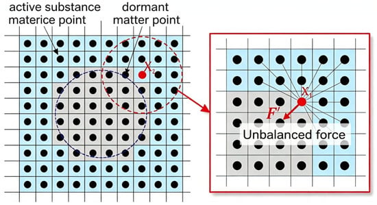
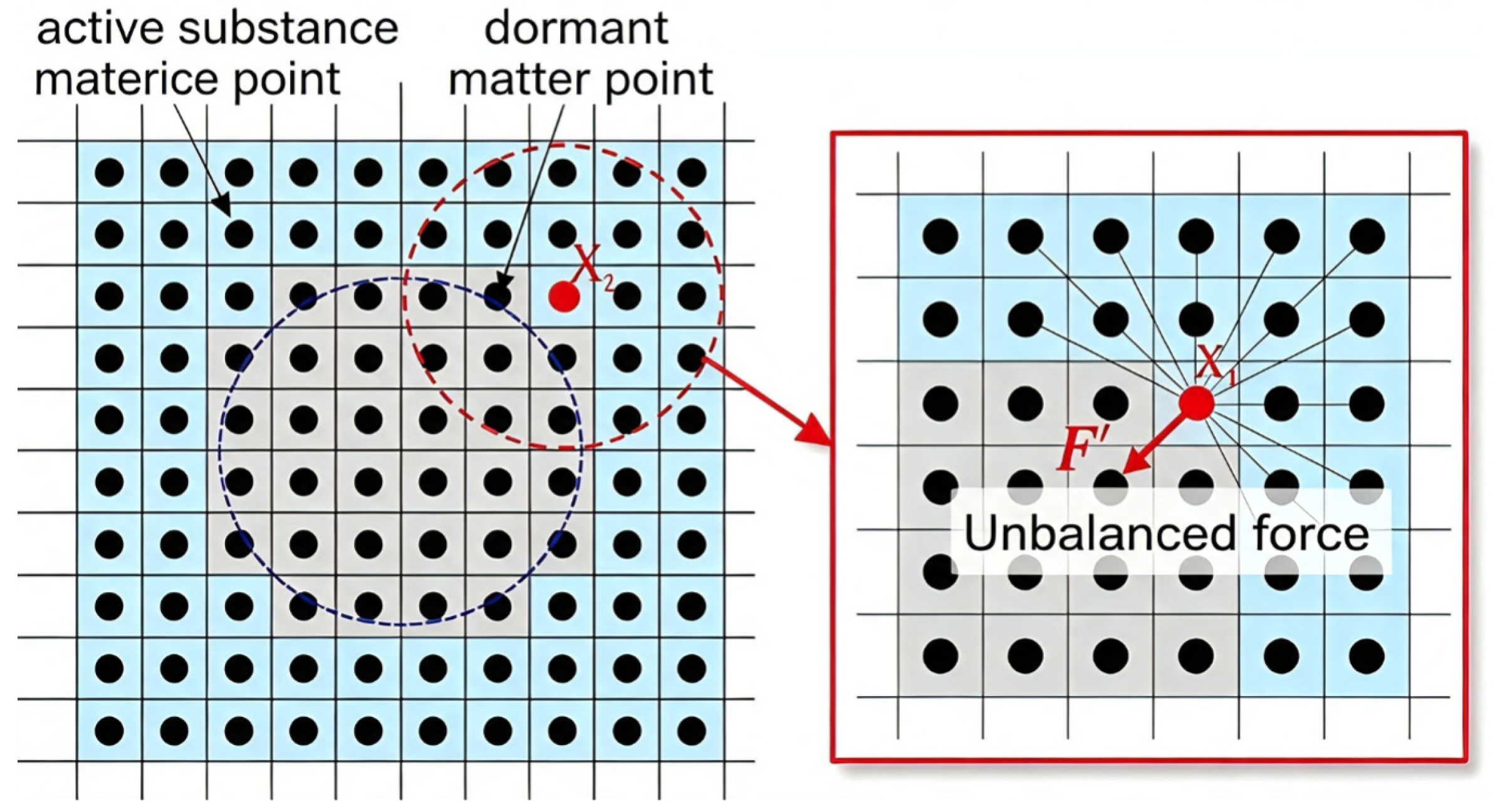
Excavation unloading is a major engineering factor that causes instability of surrounding rock in underground works such as tunnels and induces various geological disasters. To reveal the excavation unloading effect and its influence mechanism on tunnel surrounding rock stability, the material point dormancy method (MPDM) is introduced to simulate the continuous–discontinuous dynamic process of tunnel excavation [31]. As shown in Figure 2, by setting the material points in the excavation area “dormant”, i.e., cutting off the interaction forces (forces on bonds) between material points in the excavation and non-excavation areas, the excavation unloading effect of the tunnel is simulated. The interaction forces among all material points inside the excavation area disappear, while the neighborhood matrix of material points within a certain range along the excavation contour changes abruptly, generating unbalanced forces that are the main cause of damage and failure in the surrounding rock. The influence of tunnel excavation on material points far from the excavation area gradually diminishes. In addition, numerical damping is applied in the explicit time integration, so that a quasi-static equilibrium is reached after the sudden excavation.

Figure 2. Schematic diagram of the material point dormancy method.

The peridynamic material point dormancy method for simulating the tunnel excavation process can be represented using a scalar function [21,31]:

$$\psi \left[{\mathbf{x}}_i,{\mathbf{x}}_j,t\right]=\left\{\begin{array}{cc}1\hfill & \mathrm{if}{\mathbf{x}}_i\mathrm{and}{\mathbf{x}}_j\mathrm{are}\mathrm{active}\mathrm{material}\mathrm{points}\hfill \\ 0\hfill & \mathrm{if}{\mathbf{x}}_i\mathrm{or}{\mathbf{x}}_j\mathrm{is}\mathrm{a}\mathrm{dormant}\mathrm{material}\mathrm{point}\hfill \end{array}\right.$$

(11)

The peridynamic constitutive force function is then obtained:

$${\mathbf{T}}_{\left(i\right)\left(j\right)}\left[{\mathbf{u}}_{\left(j\right)}-{\mathbf{u}}_{\left(i\right)},{\mathbf{x}}_{\left(j\right)}-{\mathbf{x}}_{\left(i\right)},t\right]={\displaystyle \frac{1}{2}}\psi \left[{\mathbf{x}}_i,{\mathbf{x}}_j,t\right]A{\displaystyle \frac{{\mathbf{y}}_{\left(j\right)}-{\mathbf{y}}_{\left(i\right)}}{\left|{\mathbf{y}}_{\left(j\right)}-{\mathbf{y}}_{\left(i\right)}\right|}}$$

(12)

$${\mathbf{T}}_{\left(j\right)\left(i\right)}\left[{\mathbf{u}}_{\left(i\right)}-{\mathbf{u}}_{\left(j\right)},{\mathbf{x}}_{\left(i\right)}-{\mathbf{x}}_{\left(j\right)},t\right]=-{\displaystyle \frac{1}{2}}\psi \left[{\mathbf{x}}_i,{\mathbf{x}}_j,t\right]B{\displaystyle \frac{{\mathbf{y}}_{\left(j\right)}-{\mathbf{y}}_{\left(i\right)}}{\left|{\mathbf{y}}_{\left(j\right)}-{\mathbf{y}}_{\left(i\right)}\right|}}$$

(13)

The peridynamic basic governing equation is

$$\rho \left[{\mathbf{x}}_i\right]\ddot{\mathbf{u}}\left[{\mathbf{x}}_i,t\right]={\int }_{H_{{\mathbf{x}}_j}}\left({\mathbf{T}}_{ij}\left[{\mathbf{u}}_j-{\mathbf{u}}_i,{\mathbf{x}}_j-{\mathbf{x}}_i,t\right]-{\mathbf{T}}_{ji}\left[{\mathbf{u}}_i-{\mathbf{u}}_j,{\mathbf{x}}_i-{\mathbf{x}}_j,t\right]\right)\mathrm{d}{H}_{{\mathbf{x}}_j}+\mathbf{b}\left[{\mathbf{x}}_i,t\right]$$

(14)

The excavation also changes the seepage boundary. The tunnel is unsupported, so its surface is in contact with the atmosphere (gauge pressure zero) and acts as a drained boundary. If the scalar function $\psi$ were applied to the fluid bonds, the dormant points would be disconnected from the groundwater and the excavation surface would become an impermeable boundary, which is not the physical condition. Therefore, $\psi$ is applied only to the solid bonds (Equations (12)–(14)). For the fluid field, the dormant points ${\Omega }_{ex}$ are assigned a pore pressure of zero, and the fluid bonds attached to them are treated as fracture bonds, so that the groundwater can flow towards the excavation surface and be discharged. The peridynamic governing equation for pore–fracture dual-porosity media seepage with excavation unloading is then

$${\displaystyle \frac{\partial }{\partial t}}\left(\rho \left[{\mathbf{x}}_i\right]\phi \left[{\mathbf{x}}_i\right]\right)={\int }_{H_x}{\displaystyle \frac{\rho \left[{\mathbf{x}}_i,{\mathbf{x}}_j\right]}{\mu }}{\displaystyle \frac{4k_{ij}}{\pi {\delta }^2}}{\displaystyle \frac{\Phi \left[{\mathbf{x}}_j\right]-\Phi \left[{\mathbf{x}}_i\right]}{{∥\mathit{\xi }∥}^2}}\mathrm{d}{A}_{{\mathbf{x}}_j}+R\left[{\mathbf{x}}_i\right],$$

(15)

$$p\left[{\mathbf{x}}_i,t\right]=0\mathrm{for}{\mathbf{x}}_i\in {\Omega }_{ex},k_{ij}=k_f\mathrm{if}{\mathbf{x}}_i\in {\Omega }_{ex}\mathrm{or}{\mathbf{x}}_j\in {\Omega }_{ex},$$

(16)

where $k_{ij}$ is the permeability of the fluid bond (matrix value k for pore bonds and fracture value $k_{\mathrm{f}}$ for fracture bonds, Section 2.1). This boundary condition is imposed from the excavation step onward. The pressure at the excavated points is set to zero at the beginning of each solid step.

4. Simulation Analysis of Hydraulic Fracturing Process in Fractured Rock Masses

4.1. Simulation of Hydraulic Fracture Propagation in Fractured Rock Masses

Numerous studies have shown that natural structural planes such as joints, fractures, and faults significantly influence the propagation path of hydraulic fractures [32,33,34]. Since the strength of natural structural planes in rock masses is often much lower than that of the rock matrix, during hydraulic fracturing, not only tensile–shear failure of micro-fractures occurs within the rock matrix, but complex mechanical behaviors such as tension, shear, slip, and faulting also occur within weak structural planes such as joints and fractures. These behaviors are the main reasons for the complexity of stress distribution during hydraulic fracturing of rock masses.

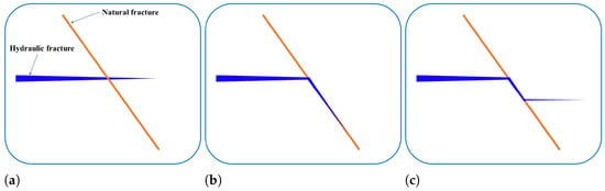
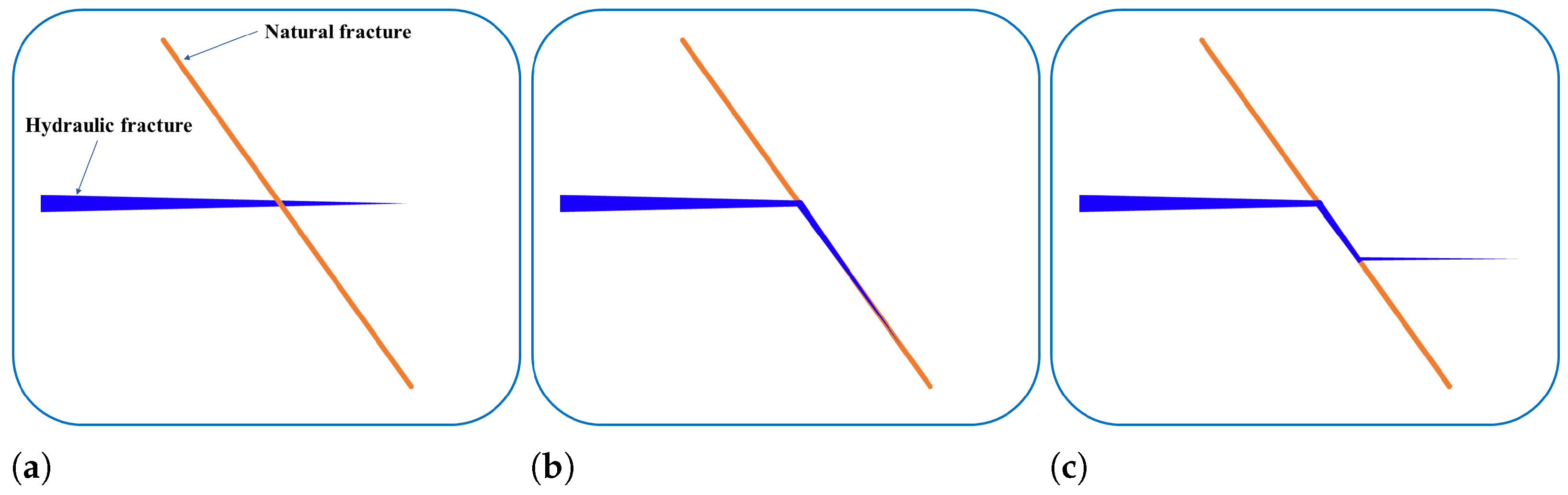
Under the influence of natural fractures, when hydraulic fractures propagate to the vicinity of natural fractures, mechanical behaviors such as shear, offset, and slip are prone to occur, leading to significant changes in the propagation path of hydraulic fractures. Existing studies [35] indicate that when hydraulic fractures encounter natural fractures, three possible scenarios may occur: (i) the hydraulic fracture crosses the natural fracture and continues to propagate; (ii) the hydraulic fracture propagates along the natural fracture for a certain distance, then re-initiates on the surface of the natural fracture and continues to propagate; (iii) the hydraulic fracture propagates along the natural fracture, as shown in Figure 3.

Figure 3. Schematic diagram of the interaction between hydraulic fractures and natural fractures. (a) Crossing; (b) Turning; (c) Re-initiating.

The mechanism by which natural fractures influence the propagation path of hydraulic fractures is very complex. According to previous experimental results [35], only under high-stress contrast and large approach angles do hydraulic fractures cross natural fractures and continue to propagate; in most cases, hydraulic fractures arrest or deflect at natural fractures. Therefore, after hydraulic fractures connect with natural fractures, their propagation path and behavior are influenced by multiple factors, including the in situ stress state, natural fracture occurrence, physical and mechanical properties of fractures and matrix, and fluid pressure [32,35].

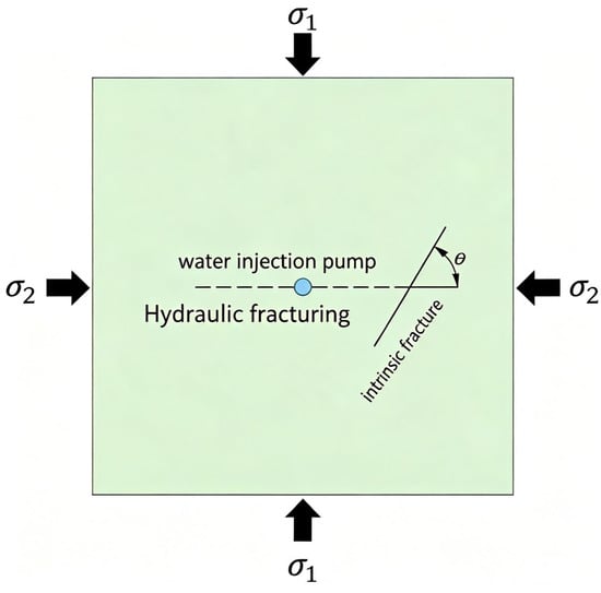
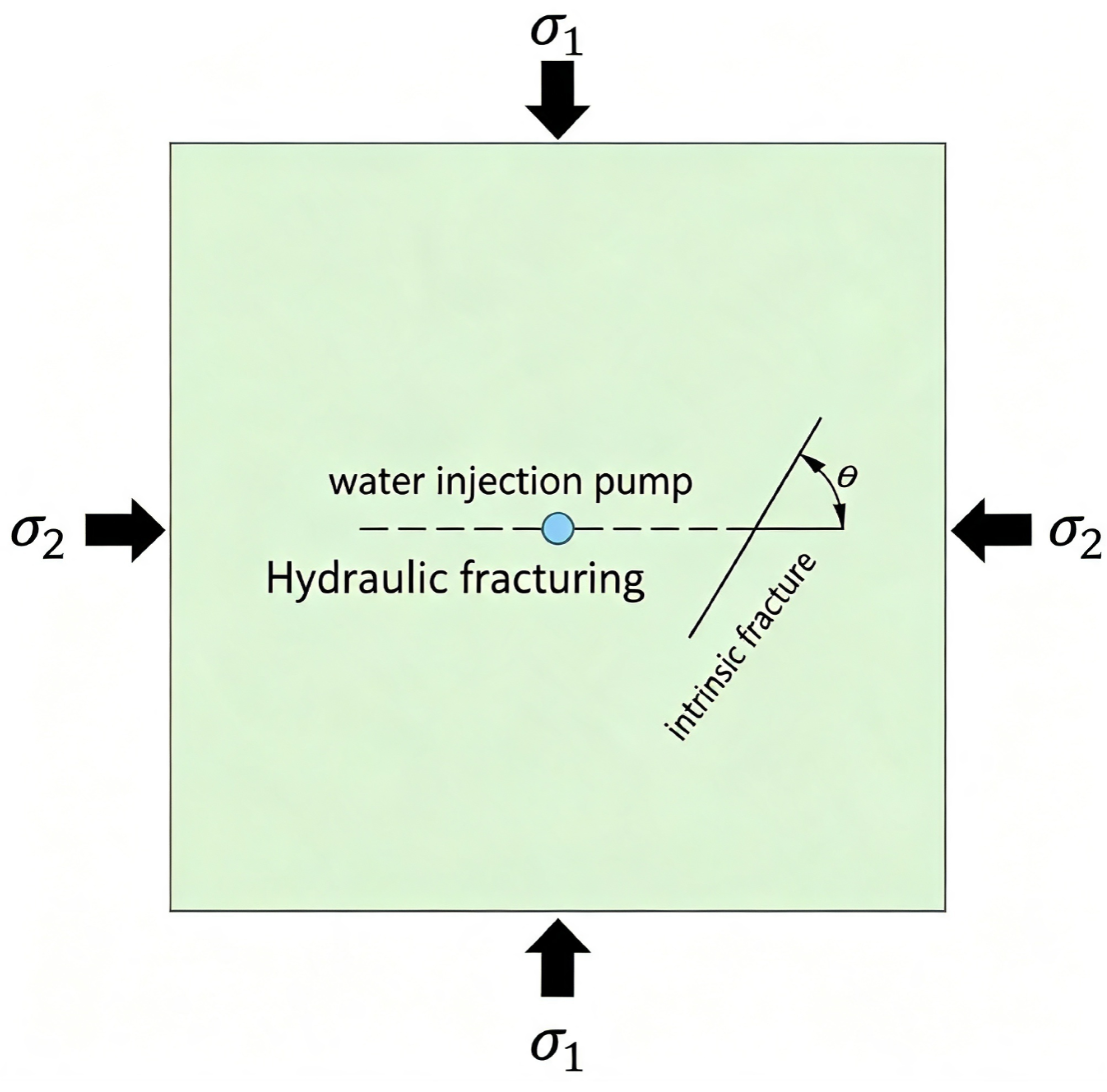
This paper focuses on the influence mechanism of natural fracture dip angle on the propagation path of hydraulic fractures during hydraulic fracturing of rock masses. As shown in Figure 4, a numerical model for hydraulic fracturing of fractured rock masses is established. The model is a rectangular area of size $64\mathrm{cm}\times 64\mathrm{cm}$, with a water injection hole of radius 3.2 cm at its centroid. Directional perforations of length 1 cm are opened (extending from the hole boundary) at the left and right ends of the injection hole. The natural fracture is 8 cm in length and its center is located 16 cm from the center of the injection hole. The center of the injection hole, the directional perforations, and the middle of the fracture are always on the same horizontal line. The confining pressure acting in the vertical direction of the model is ${\sigma }_1=10\mathrm{MPa}$, and the confining pressure in the horizontal direction is ${\sigma }_2=15\mathrm{MPa}$. Here ${\sigma }_1$ and ${\sigma }_2$ denote the vertical and horizontal confining stresses, respectively, and are not ordered as principal stresses. The model is discretized using a uniform material point spacing of 0.4 cm, resulting in a total of 25,600 material points in the core computational area. The neighborhood radius is set to 3.015 times the material point spacing, i.e., approximately 1.2 cm, and the model thickness is set to one layer of material point radius, i.e., 0.4 cm. To eliminate boundary effects, three layers of material points are set at the model boundaries as virtual boundary layers, and confining pressures are applied to these virtual boundary layers; the pore pressure in the virtual layers is fixed at zero (drained outer boundary).

Figure 4. Numerical calculation model for hydraulic fracturing of naturally fractured rock mass.

The model assumes homogeneous and isotropic properties. The material density is 2090 kg/m³, elastic modulus is 30 GPa, Poisson’s ratio is 0.25, critical stretch is 0.0005, and the Biot coefficient is set to 0.8. The porosity is 0.05 and the permeability of the fracture bonds is $1\times {10}^{-20}{\mathrm{m}}^2$ (the matrix is non-conductive in this section, i.e., only fracture bonds conduct water). These are effective parameters of the flow model: the pressure evolution depends on k, $\phi$, $\mu$ and $c_w$ only through the combination $k/\left(\phi \mu c_w\right)$. The fluid density is set to 1000 kg/m³, viscosity coefficient to $0.899\times {10}^{-3}\mathrm{Pa}·\mathrm{s}$ (0.899 mPa·s) and compressibility coefficient to $4.85\times {10}^{-10}{\mathrm{Pa}}^{-1}$ ($4.85\times {10}^{-4}{\mathrm{MPa}}^{-1}$). Water pressure is applied to the material points inside the injection hole (radius 3.2 cm). Water pressure is applied there in a pressure increment manner at a pressure loading rate of 10 kPa/s (10 kPa per solid time step, with a nominal time step of 1 s). The solution process adopts an iterative scheme, with the fluid module computing 100 time steps for each time step of the solid module. To better implement boundary stress loading, 500 solid time steps are first computed to reach the initial stress state before simulating the water injection process; 3500 solid time steps are computed in total.

To investigate the influence of natural fracture dip angle on hydraulic fractures during hydraulic fracturing, eight calculation cases are considered, including no fracture and natural fracture dip angles of 0°, 15°, 30°, 45°, 60°, 75°, and 90°, as detailed in Table 1.

Table 1. Hydraulic fracturing calculation scenarios for rock masses with natural fractures at different dip angles.

Case	Vertical Stress ${\mathit{\sigma }}_1$ (MPa)	Horizontal Stress ${\mathit{\sigma }}_2$ (MPa)	Natural Fracture Dip Angle (°)
No. 1	10	15	No fracture
No. 2	10	15	0
No. 3	10	15	15
No. 4	10	15	30
No. 5	10	15	45
No. 6	10	15	60
No. 7	10	15	75
No. 8	10	15	90

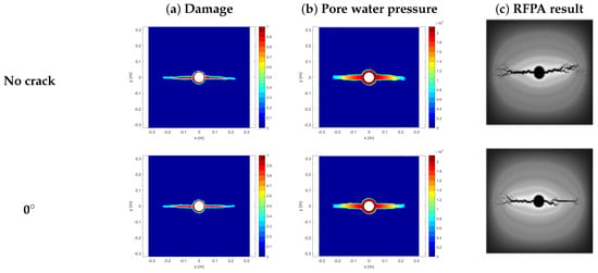
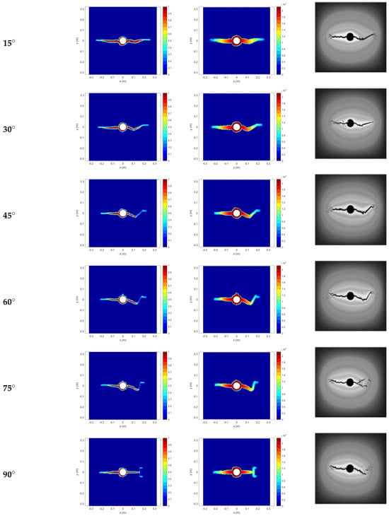
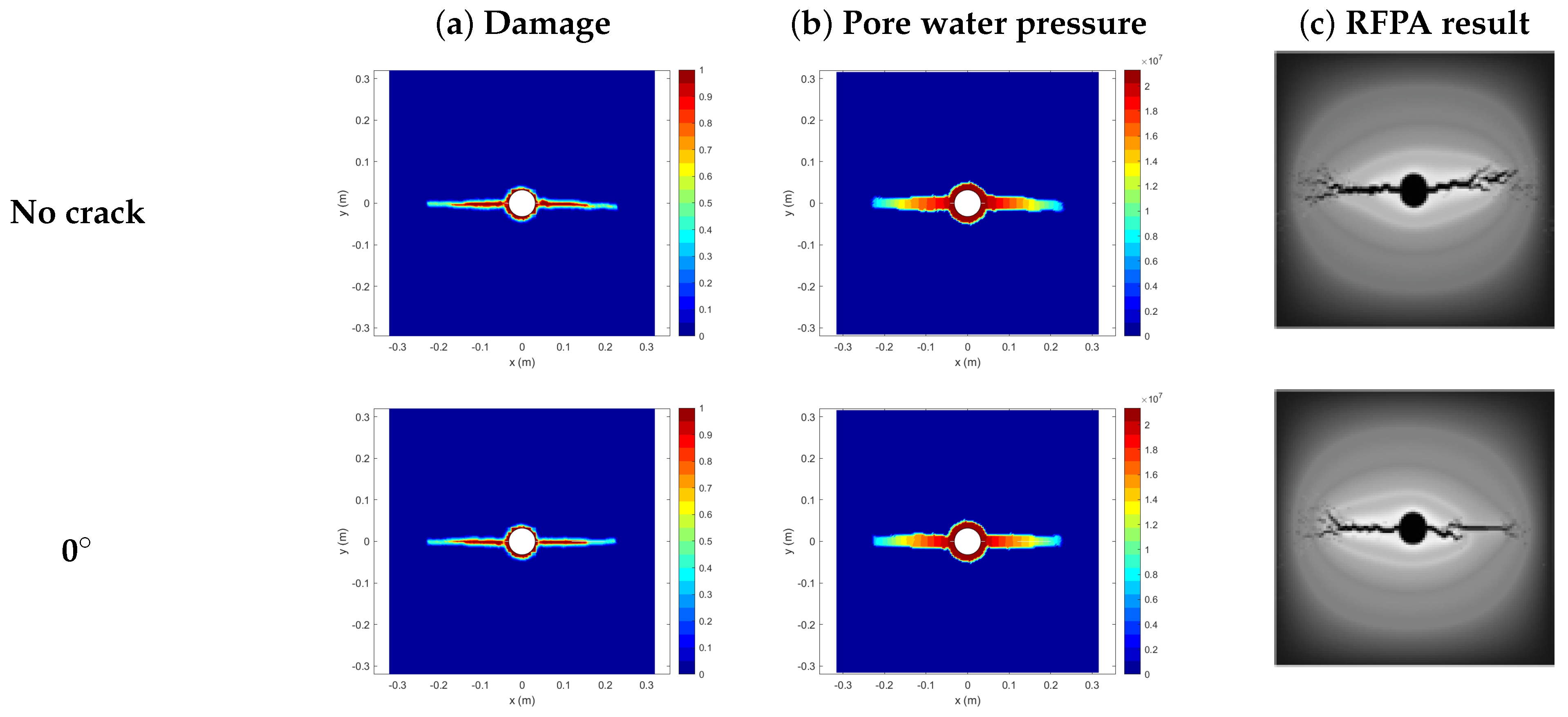
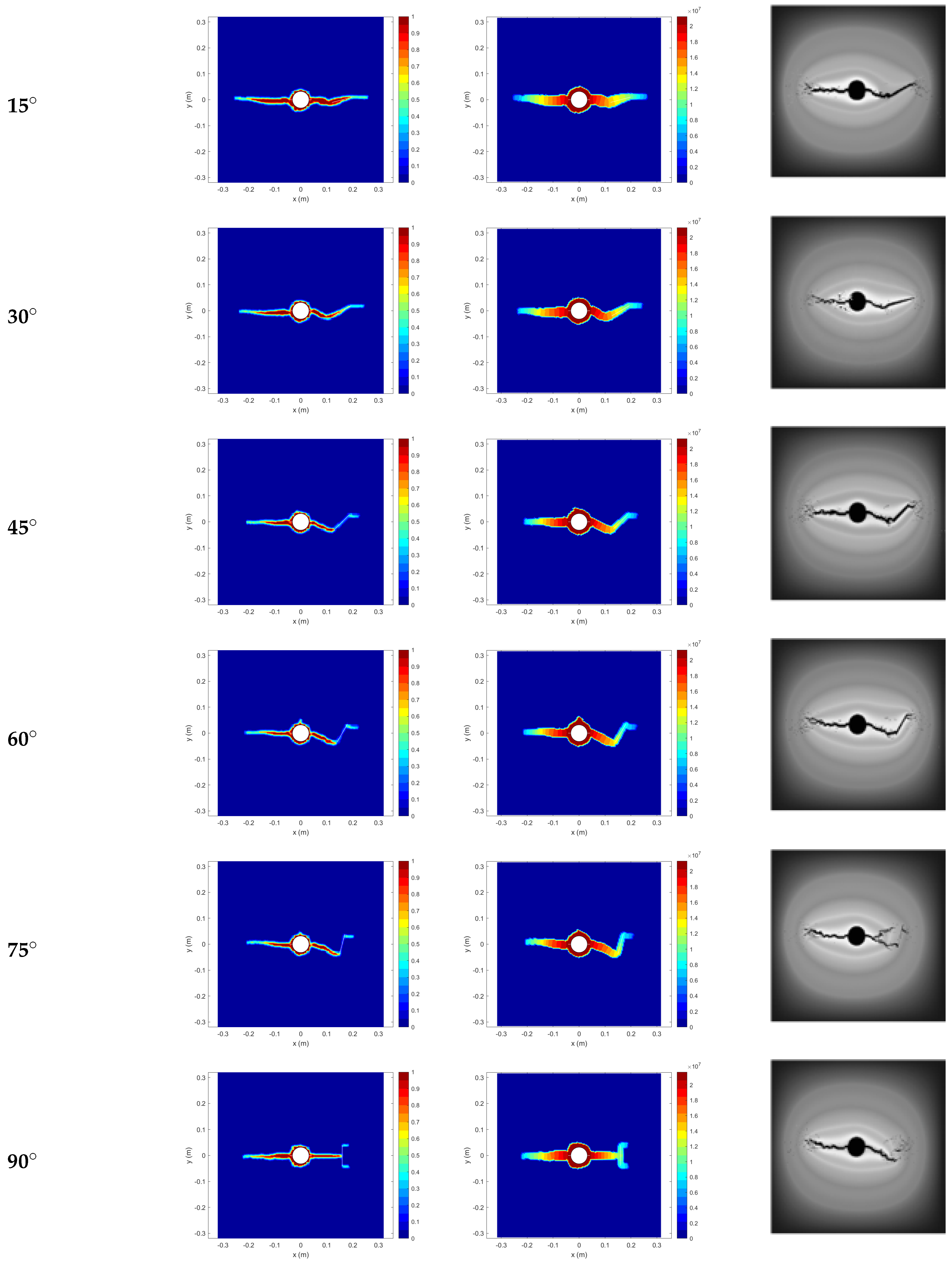
The simulation results of hydraulic fracturing of naturally fractured rock masses with different dip angles are shown in Figure 5, along with RFPA simulation results (computed by the authors with the RFPA software [36]) under the same calculation conditions. It can be observed that, in the absence of natural fractures, hydraulic fractures mainly propagate in the horizontal direction (perpendicular to the minimum principal stress direction or parallel to the maximum principal stress direction). During water injection, damage begins to appear around the injection hole due to the combined effects of pore water pressure and confining pressure. However, due to the presence of perforations, hydraulic fractures initiate from the perforations and propagate horizontally. When the natural fracture dip angle is relatively small ($\theta \le {60}^{\circ }$), because the distances from the two ends of the fracture to the injection hole differ significantly, hydraulic fractures connect with the tip of the natural fracture during propagation. Fluid enters the natural fracture through the hydraulic fracture, activating the natural fracture and generating new fractures at the distal end of the natural fracture, eventually forming a hydraulic channel that penetrates the natural fracture. The RFPA comparison is a code-to-code consistency check: it supports the qualitative fracture trajectories and the interaction modes with the natural fracture, and the instability pressures (see below), but it does not validate the physical interpretation of damage-induced permeability change or absolute magnitudes.

Figure 5. Simulation results of hydraulic fracturing of naturally fractured rock masses with different dip angles. (a) Damage distribution; (b) pore water pressure distribution; (c) RFPA simulation results computed by the authors with the RFPA software [36].

However, when the natural fracture dip angle is relatively large ($\theta \ge {75}^{\circ }$), since the peridynamic model adopts a homogeneous isotropic assumption while RFPA considers material heterogeneity and random distribution of defects using statistical distribution assumptions incorporated into numerical calculations; there are slight differences between the peridynamic and RFPA results. These differences manifest mainly in two aspects: (i) When the natural fracture dip angle is 75°, the peridynamic simulation shows that the hydraulic fracture still connects with the near end of the natural fracture and then propagates along it; in contrast, the RFPA simulation shows that the hydraulic fracture generates two secondary fractures during propagation and eventually intersects both ends of the natural fracture. (ii) When the natural fracture dip angle is 90°, due to model symmetry, the peridynamic simulation shows that the hydraulic fracture is captured by the natural fracture after reaching it, then generates two secondary fractures at both ends of the natural fracture, propagating horizontally; in contrast, the RFPA simulation shows that, due to the random distribution of grains and defects inside the rock material, one of the secondary fractures preferentially develops and connects with one end of the natural fracture.

The results indicate that during hydraulic fracturing, the natural fracture dip angle has a limited effect on the overall stability of the material. However, as the natural fracture dip angle gradually increases, the influence of natural fractures on the hydraulic fracture propagation mode gradually intensifies. For the cases examined, the homogeneous isotropic model reproduces the main fracture-path trends of the RFPA results; the differences at ${75}^{\circ }$ and ${90}^{\circ }$ are attributed to material heterogeneity. No generalization to natural rock masses is made. Nevertheless, improving the peridynamic numerical discretization method or optimizing the randomness of model parameters may help to better represent the heterogeneity of rock materials and enhance the simulation performance.

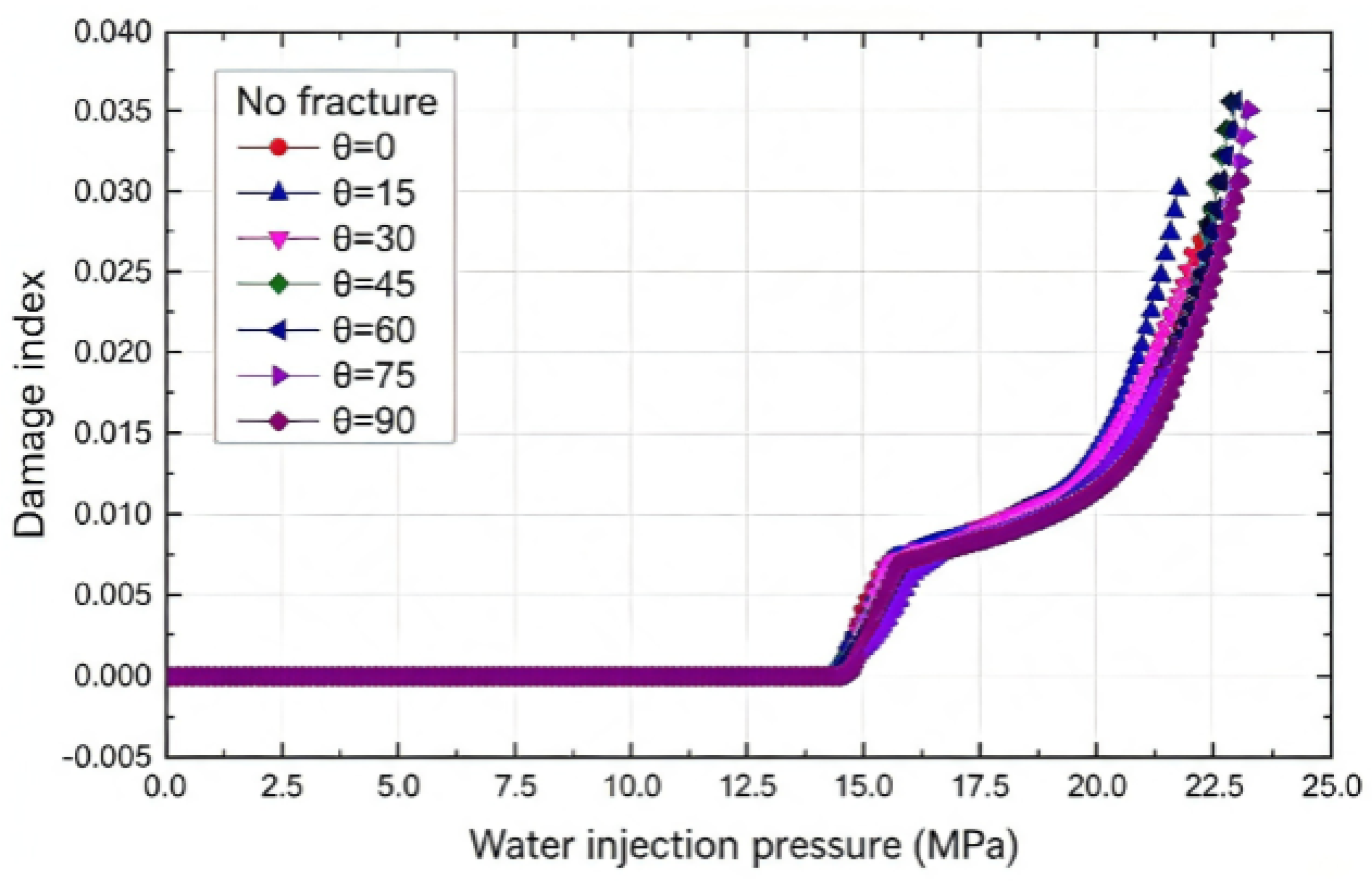
By statistically analyzing the variation of the rock damage index, the change in rock damage degree with injection pressure during hydraulic fracturing can be analyzed. The variation of damage degree in naturally fractured rock masses with different dip angles is shown in Figure 6. It can be seen that the variation of the damage index in naturally fractured rock masses with different dip angles is not significantly different from that in the fracture-free case, all increasing with the rise of injection pressure. During the increase of the rock damage index, a noticeable step phenomenon is observed, i.e., the growth rate first decreases and then increases. This is because, as the injection pressure gradually increases, the pore water pressure in the rock around the injection hole exceeds the rock strength, causing tensile failure around the injection hole first. However, due to the horizontal stress difference and the presence of directional perforations, cracking occurs at the horizontal position of the injection hole, generating hydraulic fractures that develop horizontally. After connecting with natural fractures, they continue to propagate to both ends. Eventually, when the hydraulic fracture penetrates the specimen, the rock mass undergoes instability and failure, and the rock damage degree reaches its maximum.

Figure 6. Variation of damage degree of naturally fractured rock masses with different dip angles as a function of injection pressure.

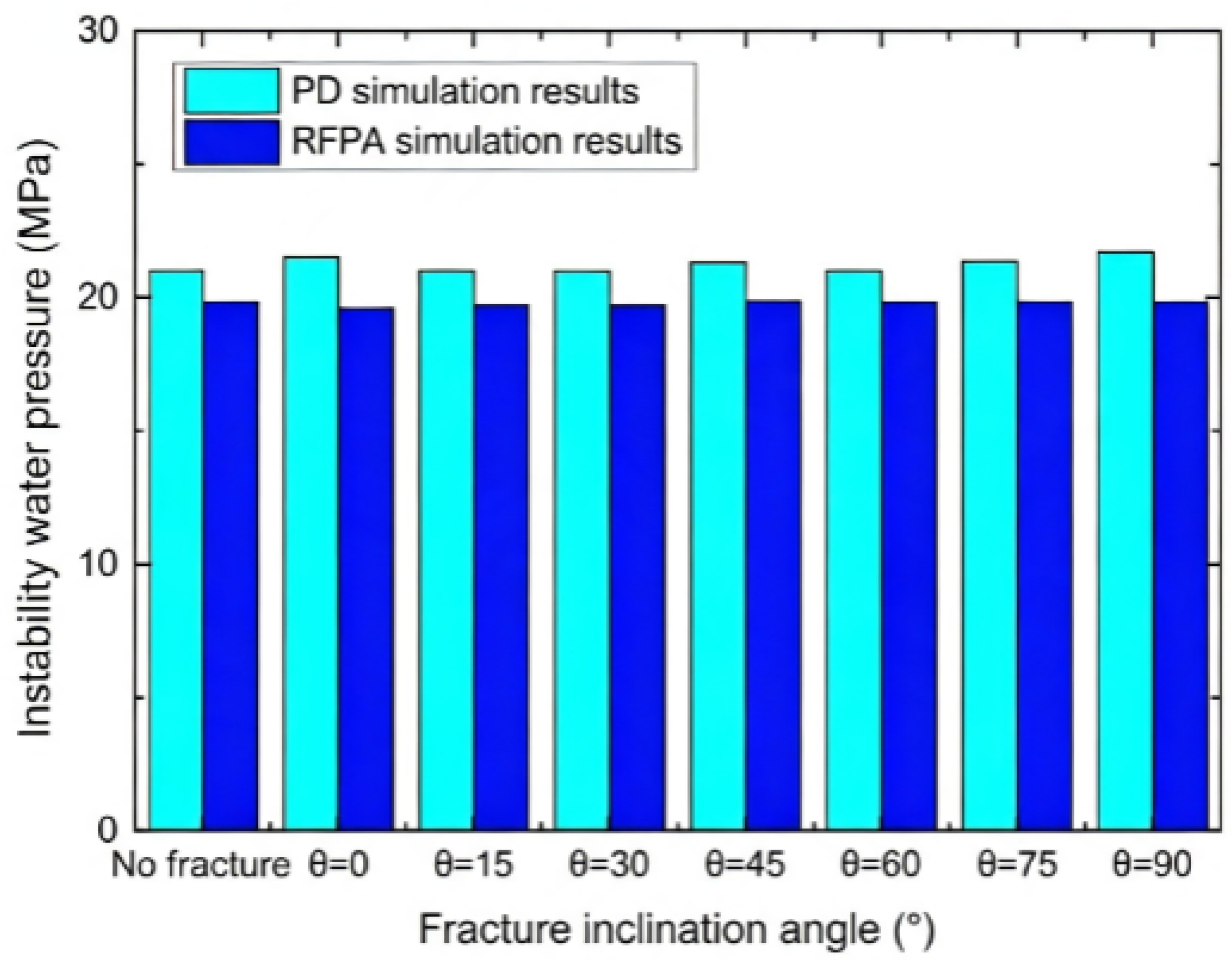
Under the same calculation conditions, the instability water pressure values obtained from peridynamic and RFPA numerical simulations are shown in Figure 7. The instability water pressure values obtained from RFPA numerical simulations are 19.8, 19.6, 19.7, 19.7, 19.89, 19.8, 19.8, and 19.8 MPa, respectively; those obtained from peridynamic numerical simulations are 21.0, 21.5, 21.0, 21.0, 21.3, 21.0, 21.4, and 21.7 MPa, respectively. The relative error between the peridynamic and RFPA numerical results (taking the RFPA result as the reference) is approximately 6–10% (6.1–9.7% for the eight cases), which is due to certain differences in the fundamental theories and model assumptions of the two numerical methods. Nevertheless, the hydraulic fracture propagation modes and rock instability states obtained are in good agreement, indicating that the peridynamic fluid–solid coupling method established in this paper can reproduce the hydraulic connection between hydraulic fractures and natural fractures during hydraulic fracturing of fractured rock masses, and the influence of natural fractures on the propagation path of hydraulic fractures, in the cases examined. Agreement between two numerical models does not by itself establish agreement with physical behavior; validation against laboratory or field data is left for future work (Section 5.4).

Figure 7. Comparison of instability water pressure in naturally fractured rock masses with different dip angles between peridynamic and RFPA simulations.

4.2. Simulation of Hydraulic Failure Process in Fractured Networks

Natural geological bodies in engineering surrounding rock are far more complex than single-fractured rock masses, having undergone multiple geological tectonic processes over long geological evolution to form intricate fracture networks. Compared with the rock matrix, joints and fractures often have lower strength and higher permeability. The presence of joints and fractures leads to pronounced heterogeneity and anisotropy of seepage in natural rock masses. Their fracture density, filling characteristics, and connectivity significantly affect the fluid seepage characteristics and structural stability of natural rock masses during hydraulic fracturing.

Existing experiments and studies [37,38] have shown that during hydraulic fracturing, fracture networks in rock masses not only easily form fluid seepage channels but also reduce the overall structural stability of the rock mass. During water injection, complex mechanical behaviors such as tension, shear, slip, and faulting occur within the natural fracture network, making it easier for hydraulic fractures to connect with natural fractures and causing deflection of hydraulic fracture propagation paths.

Joints and fractures in natural geological bodies are often randomly distributed. The propagation path of hydraulic fractures is generally governed by two prevalent factors: one is propagation along the direction of weak structural planes; the other is propagation perpendicular to the minimum principal stress direction. The fracture occurrence, cementation strength, and in situ stress state together determine the propagation trend of hydraulic fractures. To this end, this paper establishes a numerical model for hydraulic fracturing of randomly fractured rock masses and designs four calculation cases to investigate the interaction between natural fracture networks and hydraulic fractures during hydraulic fracturing of randomly fractured rock masses under different confining pressure conditions.

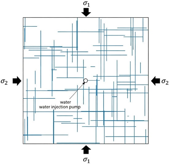
As shown in Figure 8, the numerical model for hydraulic fracturing of randomly fractured rock masses has dimensions $50\mathrm{cm}\times 50\mathrm{cm}$, with horizontal and vertical fracture sets randomly distributed.

Figure 8. Hydraulic fracturing model for randomly fractured rock mass. The injection zone is the region within about 1.5 cm of the model center.

No hole is excavated in this model. The water pressure is applied to the material points within a radius of $3.015\Delta x\approx 1.5$ cm ($\Delta x=0.5$ cm) from the model center, which forms the injection zone.

The fracture network consists of 50 horizontal and 50 vertical fractures. For each set, the midpoints of the fractures are uniformly distributed over the model area, and the fracture lengths are uniformly distributed between 0 and half of the model side length (0 to 25 cm); fractures extending beyond the model boundary are truncated. The network is a single random realization (without a fixed random seed), and the same network is used in the four cases.

Four calculation cases are set according to different confining pressures, as shown in Table 2.

Table 2. Calculation conditions for hydraulic fracturing of randomly fractured rock masses under different confining pressures. The stress ratio is defined as ${\sigma }_1/{\sigma }_2$; it is undefined for the unconfined Case No. 1.

Case	Vertical Stress ${\mathit{\sigma }}_1$ (MPa)	Horizontal Stress ${\mathit{\sigma }}_2$ (MPa)	Stress Ratio
No. 1	0	0	—
No. 2	5	10	0.5
No. 3	10	5	2.0
No. 4	10	10	1.0

The model is uniformly discretized into 10,000 material points with a material point spacing of 0.5 cm and a model thickness of 0.5 cm. The rock density is 2000 kg/m³, elastic modulus is 18 GPa, Poisson’s ratio is 0.25, critical stretch is 0.001, the porosity is 0.05, Biot coefficient is 0.8, and the fracture permeability is $1\times {10}^{-20}{\mathrm{m}}^2$. In this case the conductivity of intact bonds is set to zero, so that the flow is determined by the fracture system only (fracture-dominated limiting case of the dual-porosity model, chosen to isolate the effect of the natural fracture network on the hydraulic-fracture path). The tunnel cases in Section 5 use the full dual-porosity model with non-zero matrix conductivity. Bonds crossing a joint keep their connectivity with a stiffness factor of $0.1^n$. The fluid density is set to 1000 kg/m³, viscosity coefficient to $0.899\times {10}^{-3}\mathrm{Pa}·\mathrm{s}$ and compressibility coefficient to $4.85\times {10}^{-10}{\mathrm{Pa}}^{-1}$. Before simulating water injection, 500 solid time steps are first calculated to simulate the surrounding rock state. The pressure loading rate is 10 kPa/s (10 kPa per solid time step; pressure-controlled loading, no volumetric flow rate is prescribed), with the fluid–solid module calculating 1000 time steps for each time step of the solid module, until hydraulic fracturing of the rock mass occurs (4000 solid steps in total).

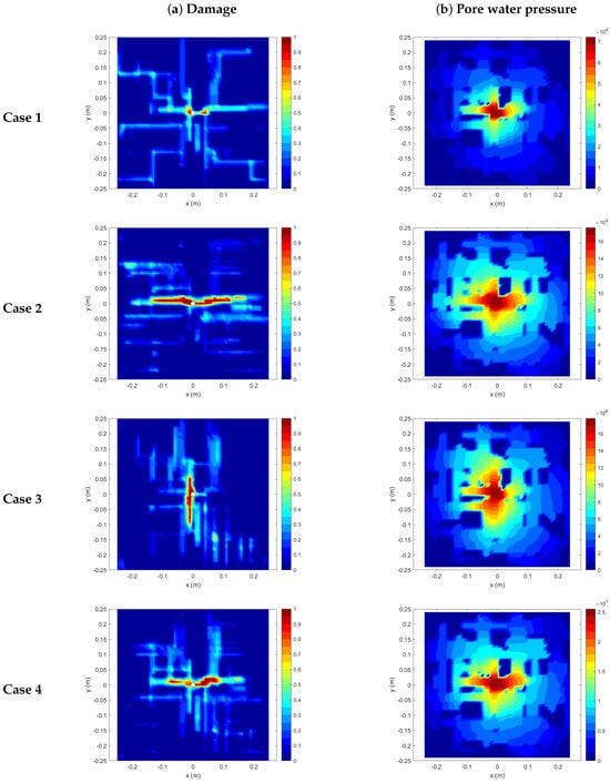
The simulation results of hydraulic fracturing of randomly fractured rock masses under different stress conditions are shown in Figure 9. Due to the good water conductivity of the natural fracture network, fluid rapidly diffuses from the injection hole into the fracture network, leading to an increase in pore water pressure in the fractured media and a decrease in effective stress. Under high injection pressure, high-stress zones first appear around the injection hole, initiating hydraulic fractures. However, the propagation path of hydraulic fractures is influenced by natural fractures; when hydraulic fractures connect with adjacent natural fractures, they propagate outward along the natural fracture network.

Figure 9. Simulation results of hydraulic fracturing of randomly fractured rock masses under different stress conditions. (a) Damage distribution; (b) Pore water pressure distribution.

Due to different confining pressure states, the fracture propagation paths differ significantly. When the stress ratio is 1.0, the confining pressure on the model is equivalent to hydrostatic pressure, and hydraulic fractures mainly propagate outward along the natural fracture network, as seen in Case No. 4 (Case No. 1 is unconfined). However, when the stress ratio is 0.5, the vertical stress is the minimum principal stress. Although hydraulic fractures are still deflected under the influence of the natural fracture network during propagation, the main fractures propagate horizontally, i.e., perpendicular to the minimum principal stress direction, as seen in Case No. 2. When the stress ratio is 2.0, the horizontal stress is the minimum principal stress, and hydraulic fractures develop vertically, as seen in Case No. 3.

The simulation results indicate that during hydraulic fracturing of naturally fractured rock masses, the propagation mode of hydraulic fractures is comprehensively influenced by the natural fracture network and stress conditions. Natural fractures, acting as preferential seepage paths, induce the propagation path of hydraulic fractures. The connection between hydraulic fractures and natural fractures activates natural fractures, thereby promoting hydraulic fracture propagation and exacerbating damage and failure of the rock material. Meanwhile, the propagation trend of hydraulic fractures is influenced by the minimum principal stress, tending to develop perpendicular to the direction of the minimum principal stress. In the cases examined, the propagation direction and path of hydraulic fractures are therefore consistent with the distribution pattern of the natural fracture network and the rock stress state. This may be of interest for guiding oil and gas extraction, in situ stress measurement, and related applications, but it has not been validated here against experiments.

Convergence with Respect to the Material-Point Spacing

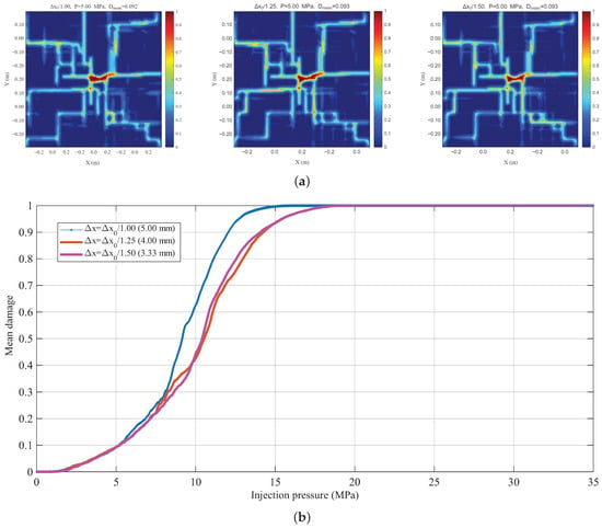
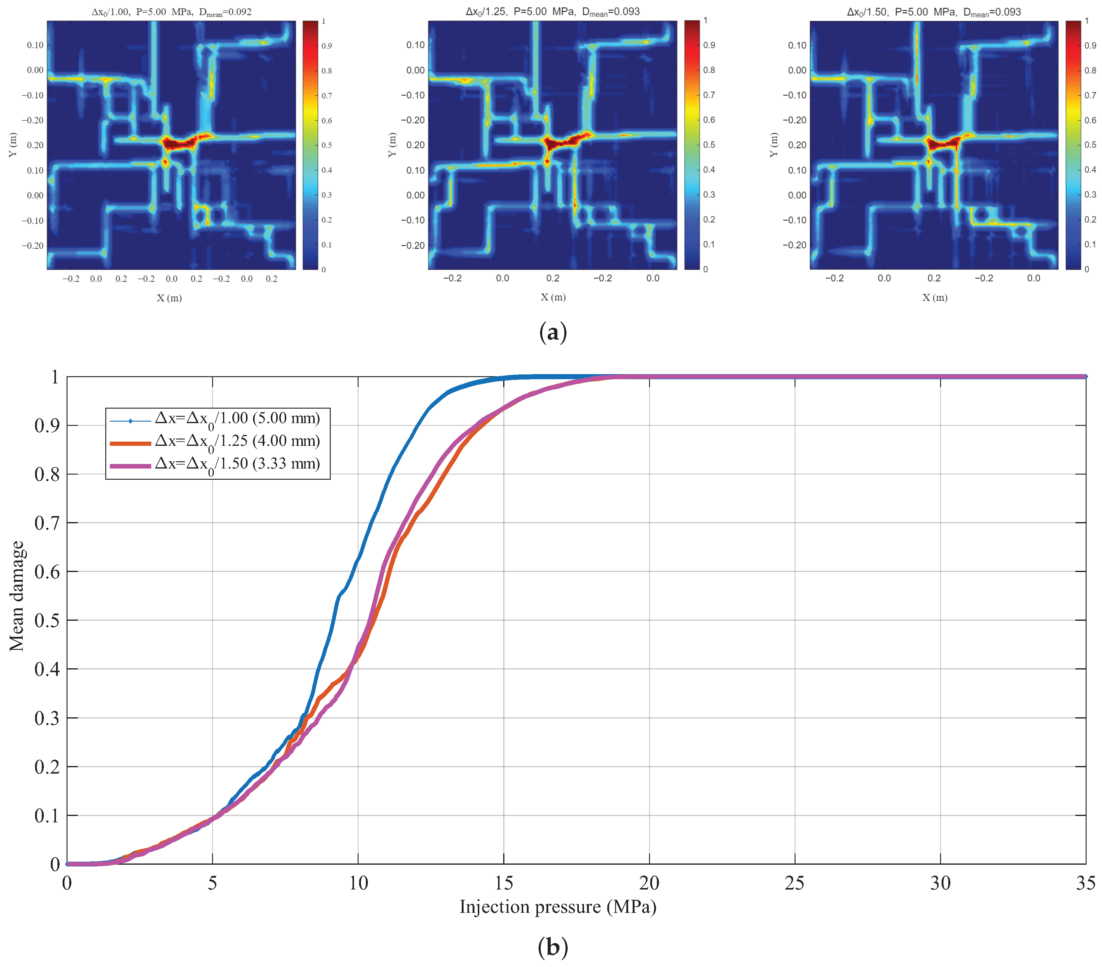
To examine the influence of the discretization, the model of this section (Case No. 4, ${\sigma }_1={\sigma }_2=10$ MPa) was simulated under the same loading condition with the material-point spacing refined by factors of 1.0, 1.25 and 1.5 relative to the spacing used above ($\Delta x=0.5$, 0.4 and 0.333 cm), at a constant horizon $\delta =3.015\times 0.5$ cm ($\delta$-convergence), so that the number of material points within the horizon increases as the spacing decreases. The same fracture network, stress conditions, loading conditions and material parameters were used in the three simulations. The case with refinement factor 1.0 corresponds to the discretization used in the simulations above.

Figure 10a compares the damage fields of the three discretizations at the same injection pressure of 5 MPa. The crack pattern is essentially unchanged: in all three cases the damage starts from the injection zone at the model center and propagates outward along the pre-existing joints, and the same set of joints is activated. The mean damage is 0.092, 0.093 and 0.093 for the refinement factors 1.0, 1.25 and 1.5, respectively. A finer discretization only gives narrower and sharper damage bands, which is the expected effect of a smaller material-point spacing. Figure 10b shows the damage degree (mean local damage $\overline{D}$, Equation (10) and the definition in Section 5.2) as a function of the injection pressure. The three curves coincide in the initial stage of fracturing and differ only slightly in the stage of rapid damage growth, where the curve for the refinement factor 1.0 lies slightly above the other two, whereas the curves for 1.25 and 1.5 are close to each other. The difference between successive refinements therefore decreases as the spacing decreases, which indicates that the damage evolution is not sensitive to the discretization within the range examined. All three curves reach the same final value once the specimen is fully damaged. The check was carried out only for this model; the tunnel models of Section 5 were not refined (Section 5.4).

Figure 10. Convergence with respect to the material-point spacing (refinement factors 1.0, 1.25 and 1.5, constant horizon). (a) Damage fields at the same injection pressure of 5 MPa; (b) damage index versus injection pressure.

5. Simulation Analysis of Excavation Damage in Surrounding Rock of Tunnels in Water-Rich Fractured Strata

5.1. Influence Mechanism of Groundwater Seepage on the Excavation Damage Zone of Tunnels

Discontinuous structural planes such as joints and fractures reduce the strength of rock masses, leading to an expansion of the damage zone in surrounding rock during tunnel excavation and increasing the risk of surrounding rock instability and collapse [31,39]. At the same time, joints and fractures are preferential channels for groundwater seepage and natural water-conducting and water-storing structures. Under saturated conditions, the effective stress of surrounding rock decreases. Under excavation unloading, joints and fractures are more prone to damage, which may lead to local or overall instability of the surrounding rock structure. Moreover, groundwater seepage greatly exacerbates surrounding rock damage, seriously affecting tunnel construction safety.

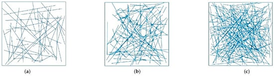
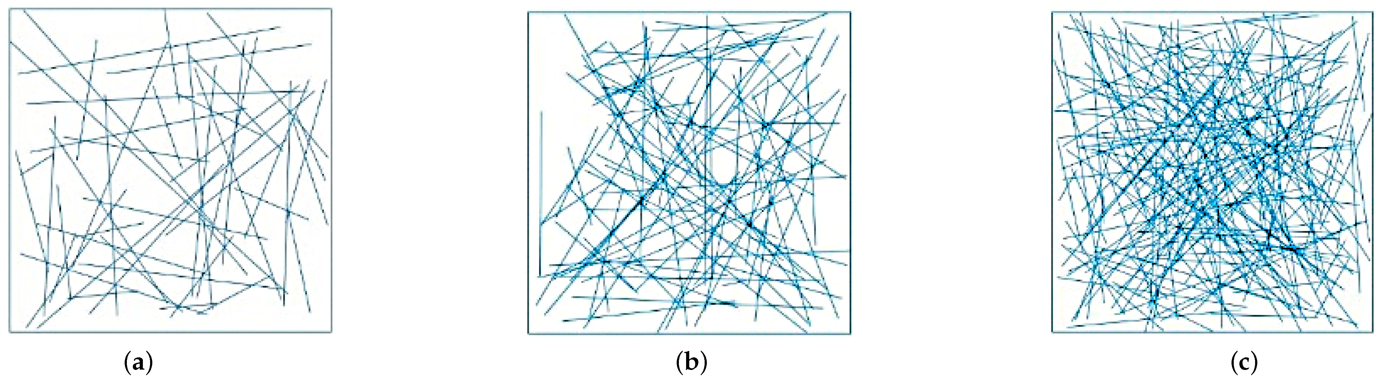
To reveal the influence mechanism of joint density on the stability of surrounding rock during tunnel excavation, four calculation cases were constructed: a uniform unfractured stratum, a stratum with 50 random joints, a stratum with 100 random joints, and a stratum with 200 random joints, as shown in Figure 11. In actual engineering, surrounding rock exists in a certain geological environment for a long time. Groundwater is stored not only in discontinuous structural planes such as joints and fractures but also in the rock matrix. Moreover, the water conductivity of the rock matrix has a non-negligible influence on the structural stability of surrounding rock. Therefore, a pore–fracture dual-porosity media model is required to simulate the groundwater seepage process.

Figure 11. Random jointed stratum models: (a) 50 joints; (b) 100 joints; (c) 200 joints.

The model data are summarized in Table 3. The model is a plane model of $40\mathrm{m}\times 40\mathrm{m}$. The tunnel has a horseshoe-shaped section formed by an upper arc of radius 5.5 m centered at the model center and a lower arc of radius 17 m centered at 14 m above the model center (width 11 m, height 8.5 m). The burial depth is 200 m. The joints are line segments that were generated randomly in advance and stored as end-point coordinates in a data file, which is read by the program; one random realization is used for each joint count.

Table 3. Model data of the tunnel excavation simulations.

Item	Value
Discretization	$400\times 400$ material points, $\Delta x=0.1$ m, horizon $3.015\Delta x$, thickness 0.1 m, three virtual boundary layers
Tunnel section	Upper arc $R=5.5$ m centered at the model center ($y\ge -2.24$ m); lower arc $R=17$ m centered at $(0,14)$ m; y from $-3$ to $5.5$ m; width 11 m
In situ stress	Burial depth 200 m; vertical stress $\rho gH\approx 5.2$ MPa ($g\approx 10$ m/s2) on the top boundary; lateral pressure coefficient 1.0 (5.2 MPa on both sides); gravity; vertical displacement fixed at the bottom
Rock	$\rho =2600$ kg/m3, $E=5$ GPa, $\nu =0.25$, $s_0=4\times {10}^{-4}$, $\alpha =0.8$; joint stiffness factor $0.1^n$
Flow	$\phi =0.05$; matrix $k=1\times {10}^{-19}$ m2; joint and broken bonds $\times 1000$ ($1\times {10}^{-16}$ m2); ${\rho }_w=1000$ kg/m3; $\mu =0.899\times {10}^{-3}$ Pa·s; $c_w=4.85\times {10}^{-10}$ Pa−1
Hydraulic conditions	Hydrostatic initial pressure (10 kPa/m). Section 5.1: top boundary 2.0 MPa, bottom boundary 2.4 MPa. Section 5.2: top boundary 0.5, 1.0, 1.5 and 2.0 MPa, with the bottom pressure always 0.4 MPa higher than the top. Zero pressure on the tunnel surface; no pressure prescribed on the lateral boundaries
Time steps	1000 solid steps of initial equilibrium; full-face excavation at step 1001; 4000 steps in total; 100 fluid steps per solid step; bond breakage allowed after step 1000

The material density of the rock mass is 2600 kg/m³, elastic modulus is 5 GPa, Poisson’s ratio is 0.25, the porosity is 0.05, Biot coefficient is set to 0.8, the permeability of the rock matrix is $1\times {10}^{-19}{\mathrm{m}}^2$, and the permeability of joints and fractures is $1\times {10}^{-16}{\mathrm{m}}^2$. The fluid density is set to 1000 kg/m³, viscosity coefficient to $0.899\times {10}^{-3}\mathrm{Pa}·\mathrm{s}$ and compressibility coefficient to $4.85\times {10}^{-10}{\mathrm{Pa}}^{-1}$. Assuming the tunnel is in a saturated state, the top of the model is subjected to a groundwater pressure of 2.0 MPa, and the bottom to a groundwater pressure of 2.4 MPa; the initial pore pressure is hydrostatic, and the difference of 0.4 MPa over the 40 m model height corresponds to the hydrostatic gradient of 10 kPa/m. An iterative solution scheme is adopted, with the fluid module calculating 100 time steps for each time step of the solid module. Before tunnel section excavation, an initial in situ stress equilibrium calculation is performed, with a cumulative total of 1000 solid time steps. Subsequently, the material point dormancy method is used to simulate the tunnel excavation unloading process. The tunnel surface is set to an unsupported condition, i.e., the tunnel surface is in direct contact with the outside, and the pore water pressure at the excavated points is reset to zero at the beginning of each solid step, so that the tunnel surface acts as a free seepage boundary.

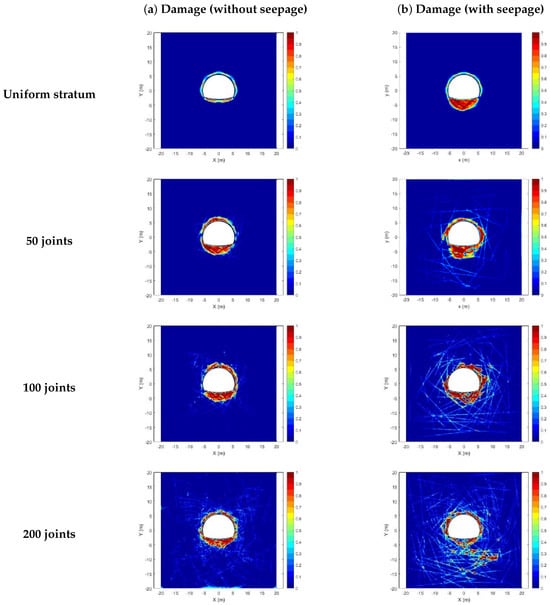
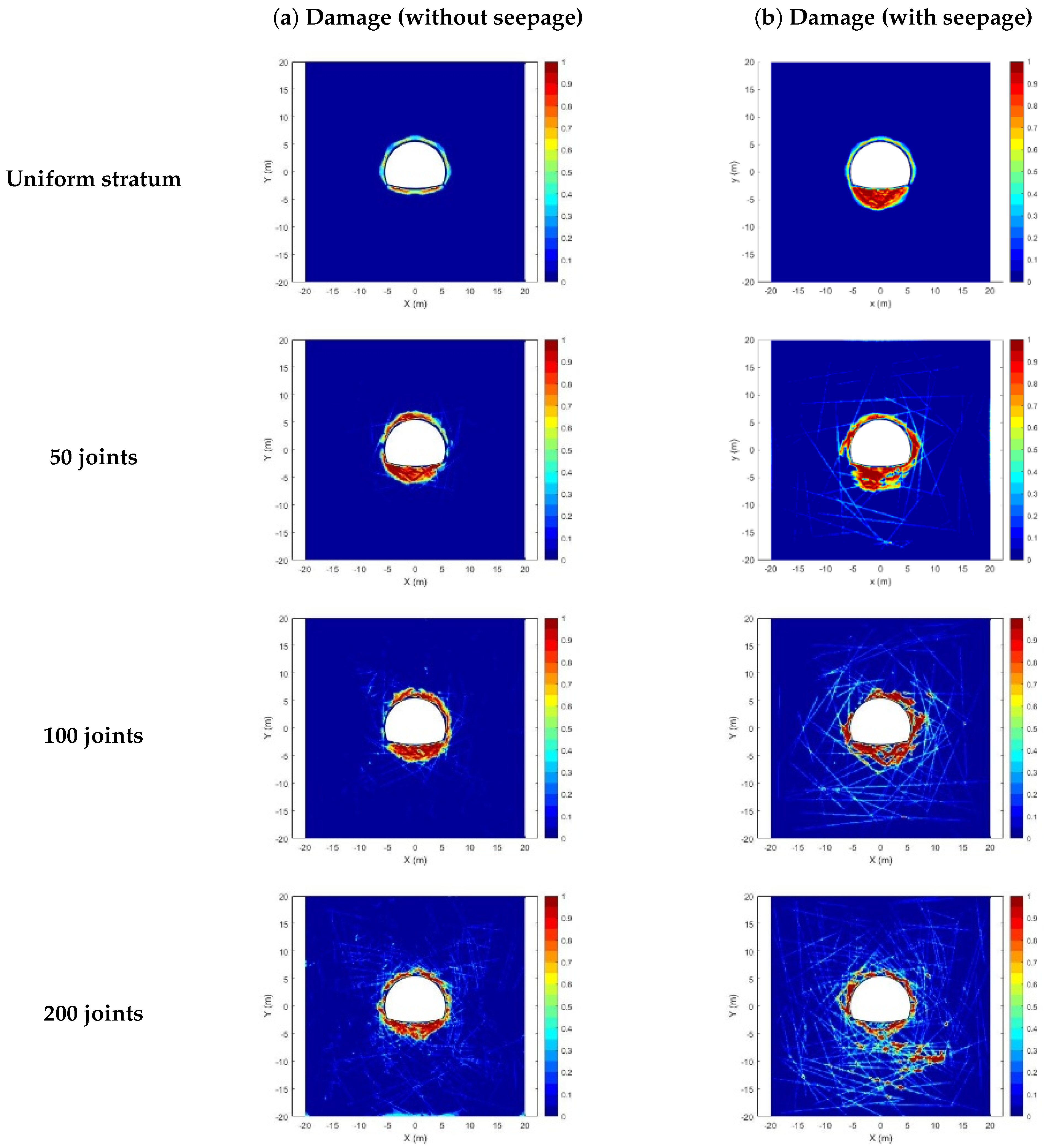
The distribution of the excavation damage zone in the surrounding rock under different joint densities is shown in Figure 12. The calculation results of the excavation damage zone in jointed strata without considering seepage are also provided for comparison and reference. By comparison, it can be seen that under the action of seepage, the influence range of the excavation damage zone is wider and mostly distributed on or near the joint surfaces. This indicates that joints and fractures are more susceptible to the unloading effect of tunnel excavation, thereby reducing the overall structural stability. During tunnel excavation, not only is the stress equilibrium state of the surrounding rock broken, causing significant damage to the surrounding rock near the tunnel surface, but the stability of the groundwater seepage field is also affected. This leads to seepage stress in the groundwater stored in joints and fractures, causing changes in the effective stress in a wider range of surrounding rock. By comparing the distribution of the excavation damage zone and the variation of pore water pressure in surrounding rock under different joint densities, it is clear that in the realizations examined, as joint density increases, the extent of the excavation damage zone becomes wider, and the influence of the groundwater seepage field also expands. Since tunnel support is not considered, the tunnel surface is a free seepage boundary. As joints and fractures are preferential channels for groundwater seepage, their pressure drop is more pronounced than that of the rock matrix. The pressure gradient between joints/fractures and the rock matrix generates local unbalanced forces, further exacerbating the damage and failure of surrounding rock.

Figure 12. Calculation results of rock stability in jointed strata under seepage action. (a) Damage distribution without seepage; (b) damage distribution with seepage.

5.2. Influence of Seepage Pressure on Excavation Damage of Tunnels

Groundwater seepage seriously affects the stability of surrounding rock during tunnel excavation, exacerbates the degree of surrounding rock damage, and expands the disturbance range of excavation unloading on the surrounding rock stress field and seepage field. Therefore, the distribution range of the excavation damage zone and the seepage laws of surrounding rock in jointed strata under different seepage pressure conditions are studied next.

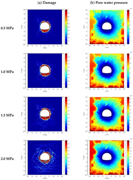
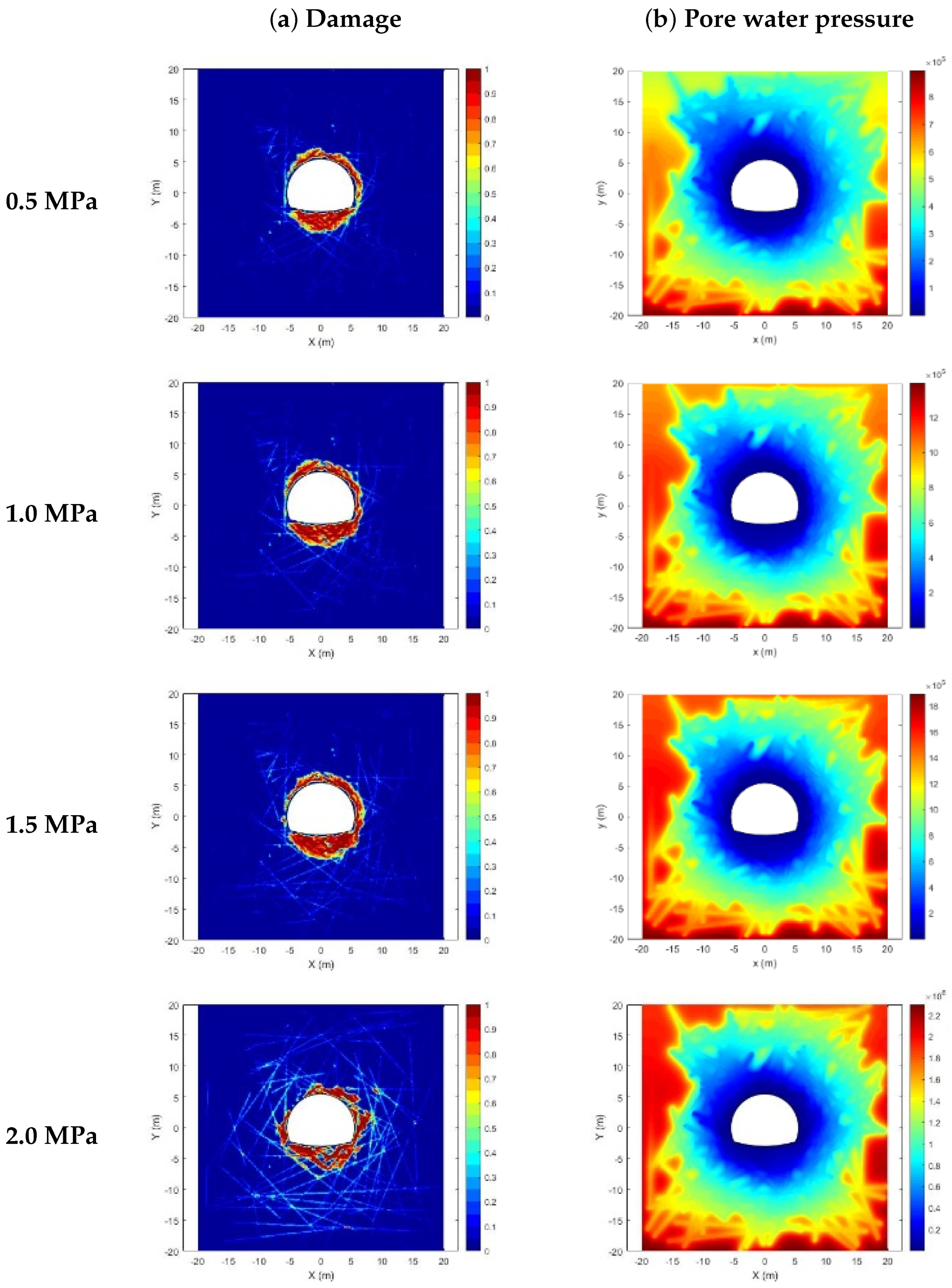
With other parameters kept constant, four calculation cases were set by adjusting the pressure boundary condition at the top of the model: 0.5 MPa, 1.0 MPa, 1.5 MPa, and 2.0 MPa. The pressure at the bottom boundary was changed together with the top, so that the pressure difference of 0.4 MPa between them (the hydrostatic gradient of 10 kPa/m over the 40 m model height) remained constant. The study therefore changes the groundwater head above the model at a constant hydraulic gradient, and isolates the influence of the absolute seepage pressure. The lateral boundaries have no prescribed pressure. The pore–fracture dual-porosity media model was used to simulate the excavation process of a 100-random-joint stratum. The 2.0 MPa case is the same calculation as the 100-joint case with seepage in Figure 12. The calculated results of the excavation damage zone and pore water pressure are shown in Figure 13.

Figure 13. Calculation results of rock stability of jointed strata under different seepage pressure conditions. (a) Damage distribution; (b) pore water pressure distribution.

The simulation results show that the distribution range of the excavation damage zone expands with increasing seepage pressure. The surrounding rock near the tunnel is severely damaged, while damage in the farther surrounding rock is mainly distributed on or near joint surfaces. Since the geological structure of the calculation model is identical, the variation pattern of the seepage field in the surrounding rock after excavation is similar, with pore water pressure decreasing from the periphery toward the tunnel interior. However, due to different initial seepage pressures, the pore water pressure at the same location in the surrounding rock varies. Under high seepage pressure, the pore water pressure in the surrounding rock is higher. With the total stress of the surrounding rock remaining constant, the effective stress decreases. The seepage pressure on joints and fractures is more likely to exceed the strength limit, causing tensile or shear failure of joints and fractures, thereby exacerbating the damage and failure of surrounding rock. The damage distribution also shows that under high seepage pressure, micro-fractures formed within the tunnel surrounding rock develop deeper, further expanding the distribution range of the excavation damage zone.

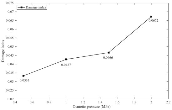
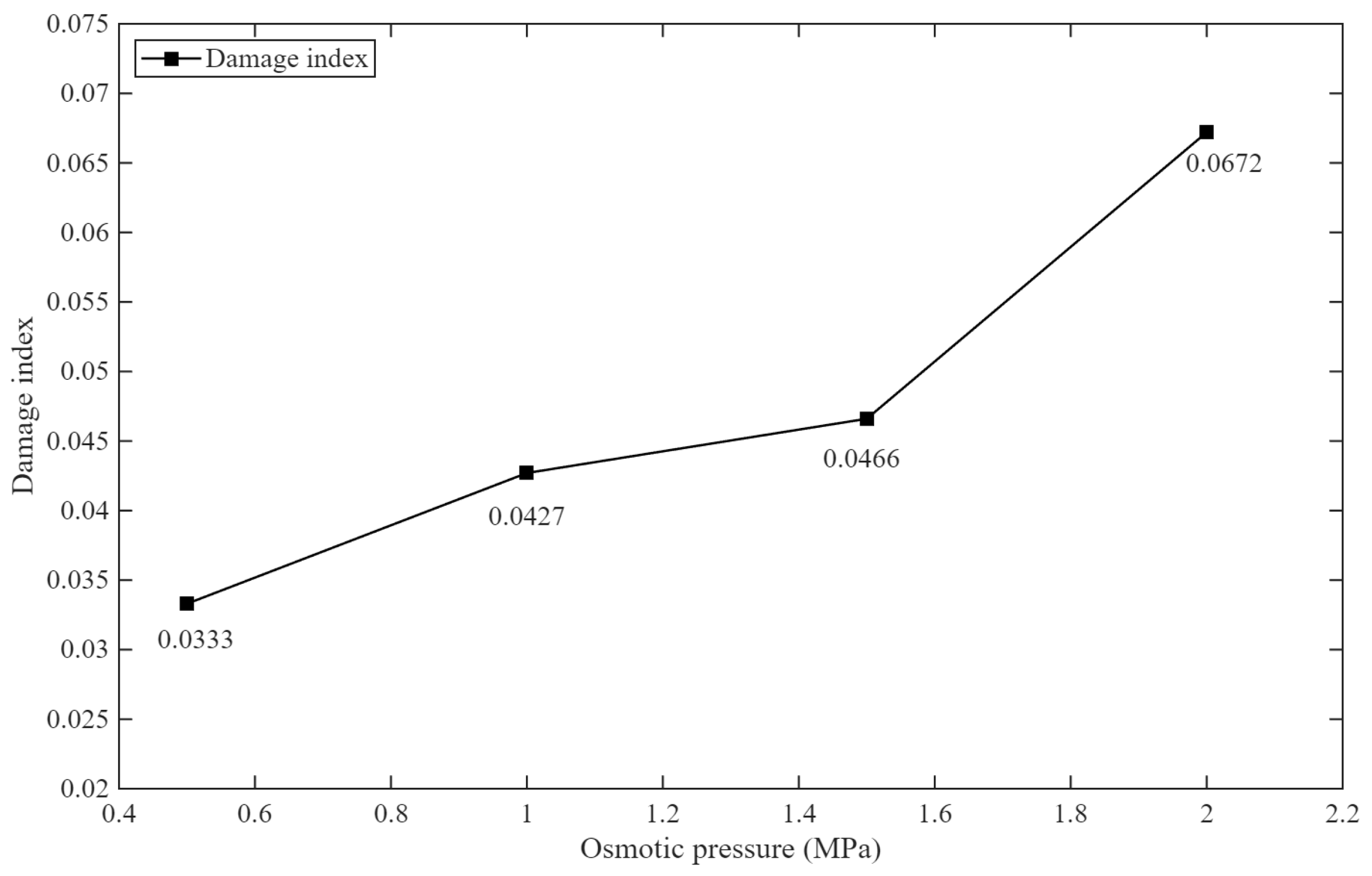
Figure 14 shows the variation of the damage degree of tunnel surrounding rock under different seepage pressure conditions. The damage degree is defined as the mean value of the local damage D (Equation (10)) over all material points, $\overline{D}={\displaystyle \frac{1}{N}}{\sum }_{i=1}^N{D}_i$, which is an area-weighted measure of the extent of the damage zone. It can be seen that the damage degree of tunnel surrounding rock increases with the increase of seepage pressure. Excavation unloading not only causes damage and failure of the rock mass near the tunnel but also damages distant joints and fractures, thereby increasing the damage degree of surrounding rock. Moreover, under high seepage pressure, joints and fractures farther from the tunnel are more likely to be activated. Therefore, when excavating tunnels in water-rich fractured strata, the influence of seepage pressure should be considered in the tunnel construction scheme.

Figure 14. Damage degree of surrounding rock in jointed strata under different seepage pressure conditions.

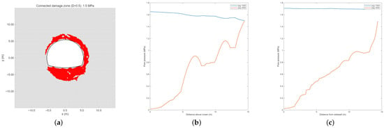
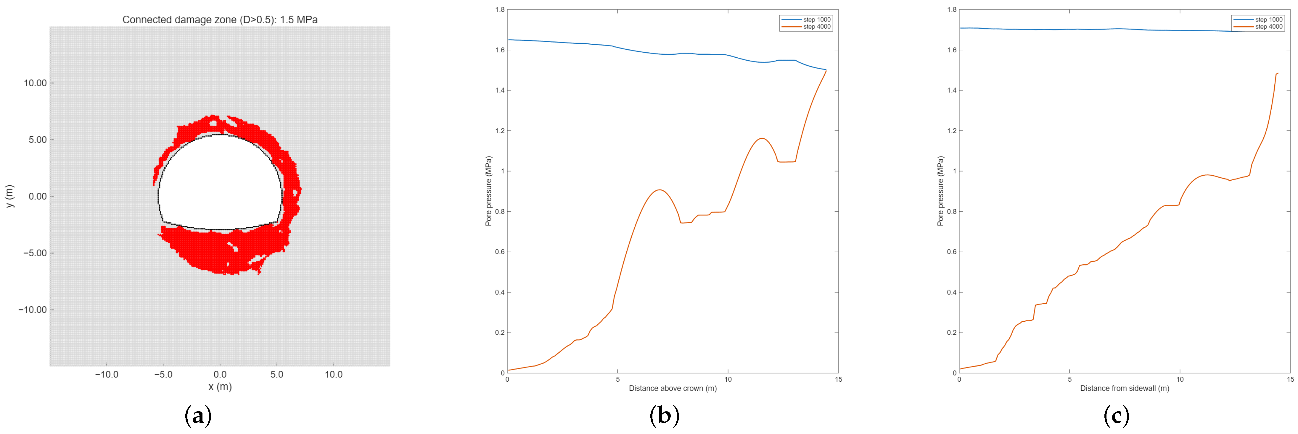
To describe the spatial distribution of damage around the tunnel, the damaged points ($D>0.5$) connected to the tunnel boundary were extracted for the 1.5 MPa case after excavation (Figure 15a). The damage zone has a mean depth of about 1.8 m, and its maximum depths at the arch, sidewalls and invert are about 1.7, 1.7 and 4.1 m, respectively; i.e., the damage penetrates much deeper at the invert. This ranking is insensitive to the damage threshold (0.25–0.9), whereas the area and the mean depth are more sensitive to it. The damage zone has an area of about 55 m². With thresholds of 0.25–0.9, the maximum depths are 1.5–1.9 m (arch), 1.3–2.0 m (sidewalls) and 3.7–4.8 m (invert). The corresponding indicators for all three seepage-pressure cases are summarised in Table 4; the EDZ area and maximum invert depth increase monotonically with the seepage pressure. Before excavation, the pore pressure follows the hydrostatic distribution; after excavation, it drops to nearly zero at the tunnel wall and recovers gradually with the distance from the wall, forming a depressurized zone around the tunnel (Figure 15b,c).

Figure 15. Quantitative description of the excavation damage zone and pore-pressure distribution for the 1.5 MPa case of Section 5.2. (a) Damage zone connected to the tunnel boundary ($D>0.5$, red); (b) pore-pressure profile along the vertical line above the crown; (c) pore-pressure profile along the horizontal line outside the sidewall. Profiles are shown before and after excavation.

Table 4. Quantitative characterisation of the excavation damage zone for the three seepage-pressure cases (lateral pressure coefficient $K_0=1$, burial depth 200 m, 100 random joint sets; damage threshold $D>0.5$; region connected to the tunnel boundary).

Seepage Pressure	EDZ Area (m2)	Max. Depth, Arch (m)	Max. Depth, Sidewalls (m)	Max. Depth, Invert (m)
0.5 MPa	42.1	1.72	1.52	3.41
1.0 MPa	53.3	2.15	1.56	3.90
1.5 MPa	54.9	1.72	1.75	4.13

5.3. Computational Cost

All simulations were run with a serial MATLAB R2025a implementation on a workstation (Intel Core i9-10940X CPU, 3.30 GHz; 256 GB RAM; Windows 11). The computing time was about 1 h 40 min for the hydraulic fracturing model of Section 4.1, about 3.5 h for the random-fracture model of Section 4.2, and about 23 h 10 min for the tunnel model of Section 5.

5.4. Limitations and Scope of Applicability

Homogeneous and isotropic matrix. The rock matrix has uniform elastic modulus, critical stretch and conductivity; joints enter only through a stiffness reduction factor and a conductivity multiplier of the bonds crossing them. Heterogeneity, which governs fracture initiation sites and branching, is not represented; this is consistent with the differences from the RFPA results at ${75}^{\circ }$ and ${90}^{\circ }$. A homogeneous matrix tends to produce more symmetric fracture paths and may bias the instability pressure. In the jointed models, flow and damage are controlled by the prescribed joint geometry and the assigned joint conductivity; aperture and roughness variability and matrix anisotropy are not represented.

Two-dimensional model. The model represents a cross-section of a long tunnel. It neglects longitudinal stress redistribution, the three-dimensional arching effect ahead of the face, out-of-plane flow and the three-dimensional connectivity of joint networks (two-dimensional networks are less connected than three-dimensional ones at equal density).

Parameters and validation. The flow parameters are effective values of the numerical model and the time of the fluid solver is a numerical (quasi-static) time. The results are therefore interpreted in terms of pressure distributions and damage patterns, not real time or real inflow rates. The comparison with RFPA is a code-to-code check; no comparison with laboratory or field data was made. The random fracture network of Section 4.2 and the tunnel joint networks of Section 5 (one realization per joint count) are single realizations. A convergence check with respect to the material-point spacing at a constant horizon was carried out only for the model of Section 4.2; the tunnel models of Section 5 were not refined because of their computing time (Section 5.3), and the influence of the horizon size was not studied. The damage thresholds used for the damage-zone indicators (0.5, with 0.25–0.9 for a sensitivity check) are conventional choices and are not calibrated against measurements.

Scope. In the cases examined, the relative trends (damage zone growing with joint density and with seepage pressure, fractures propagating perpendicular to the minimum principal stress) are the transferable result. Absolute pressures, damage extents and inflows should not be transferred directly to field conditions.

6. Conclusions

This paper addresses the numerical simulation challenge of excavation damage in surrounding rock of tunnels in water-rich fractured strata. A peridynamic pore–fracture dual-porosity media seepage model and the material point dormancy method are established. The consistency of the proposed approach with RFPA results computed by the authors is examined through typical examples, and multi-case analyses are conducted to investigate the excavation damage zone in water-rich fractured surrounding rock. The main conclusions are as follows:

• Based on the nonlocal concept of peridynamics, a pore–fracture dual-porosity media seepage model is established by equivalently treating fluid bonds as a combination of pore fluid bonds and fracture fluid bonds. Combined with the effective stress principle, a material point dual-cover theoretical model is proposed, achieving peridynamic simulation of stress–seepage coupling in fractured rock masses.
• Numerical simulations of hydraulic fracturing in rock masses with a natural fracture and with natural fracture networks were conducted for different natural fracture dip angles and stress states. In the cases examined, the natural fracture dip angle influences the propagation of hydraulic fractures, and the instability pressures and fracture paths are consistent with the RFPA results (differences of about 6–10%). The propagation mode of hydraulic fractures is comprehensively influenced by the natural fracture network and stress conditions. The propagation trend of hydraulic fractures is affected by the minimum principal stress, tending to develop perpendicular to the direction of the minimum principal stress.
• Tunnel excavation causes a sharp drop in pore water pressure in the surrounding rock within a certain range. Compared with the rock matrix, the pressure drop in fractures is more pronounced. In the cases examined, groundwater seepage exacerbates the degree of surrounding rock damage caused by excavation, and the extent of the excavation damage zone increases with joint density. As the initial seepage pressure of the surrounding rock increases, the mean damage degree shows a clear upward trend.

These conclusions are supported by the simulated configurations only. The model is two-dimensional, homogeneous and isotropic, and does not include tunnel support; the flow parameters are effective values of the numerical model; no validation against experimental or field data was performed; and the discretization check was limited to the model of Section 4.2 (Section 5.4). Further investigations are warranted to address these aspects.

Appendix A.1. Notation

Let $p_i^{\left(n\right)}$ denote the pressure at material point i at the beginning of sub-step n, and let $\mathcal{F}\left(i\right)$ denote the set of neighbours of i. The pressure of point i is updated as

$$p_i^{(n+1)}=p_i^{\left(n\right)}+\Delta p_i,\Delta p_i=\sum _{j\in \mathcal{F}\left(i\right)}{C}_{ij}\left({\tilde{p}}_j-{\tilde{p}}_i\right),$$

(A1)

where ${\tilde{p}}_j=p_j^{(n+1)}$ if j has already been updated in the current sub-step and ${\tilde{p}}_j=p_j^{\left(n\right)}$ otherwise, and the flux coefficient is

$$C_{ij}={\displaystyle \frac{2k_{ij}}{\pi \delta \phi \mu c_w{\left|{\mathit{\xi }}_{ij}\right|}^3}}A\Delta t_f,$$

(A2)

where $k_{ij}$ is the bond permeability, A is the material-point cross-sectional area, and $\Delta t_f$ is the fluid sub-step size. By construction $C_{ij}=C_{ji}$.

Appendix A.2. Reference Scheme (Jacobi)

If all fluxes were evaluated at the same time level $p^{\left(n\right)}$ (Jacobi update), the global pressure increment would satisfy

$${\displaystyle \sum _{i=1}^N}\Delta p_i^{\mathrm{J}}=\sum _i\sum _{j\in \mathcal{F}\left(i\right)}{C}_{ij}\left(p_j^{\left(n\right)}-p_i^{\left(n\right)}\right)=0,$$

(A3)

where the last equality follows from $C_{ij}=C_{ji}$ by exchanging summation indices. The Jacobi scheme is therefore globally mass-conservative.

Appendix A.3. Actual Scheme (Gauss–Seidel)

In the implemented scheme, material points are traversed in index order. When point i is updated, points $j<i$ (set $\mathcal{L}\left(i\right)$) have already received their increments $\Delta p_j^{\mathrm{GS}}$, while points $j>i$ (set $\mathcal{U}\left(i\right)$) still carry $p_j^{\left(n\right)}$. The increment of point i is therefore

$$\Delta p_i^{\mathrm{GS}}=\sum _{j\in \mathcal{L}\left(i\right)}{C}_{ij}\left(p_j^{\left(n\right)}+\Delta p_j^{\mathrm{GS}}-p_i^{\left(n\right)}\right)+\sum _{j\in \mathcal{U}\left(i\right)}{C}_{ij}\left(p_j^{\left(n\right)}-p_i^{\left(n\right)}\right).$$

(A4)

Summing over all i and using Equation (A3) to cancel the terms evaluated at $p^{\left(n\right)}$, the global residual reduces to

$$R^{\left(n\right)}\equiv {\displaystyle \sum _{i=1}^N}\Delta p_i^{\mathrm{GS}}={\displaystyle \sum _{i=1}^N}\sum _{j\in \mathcal{L}\left(i\right)}{C}_{ij}\Delta p_j^{\mathrm{GS}}.$$

(A5)

Equation (A5) shows that the residual is driven entirely by the increments of already-updated neighbours; it vanishes when $\Delta p_j^{\mathrm{GS}}=0$ for all j, i.e., at steady state.

Appendix A.4. Upper Bound

Taking the absolute value and noting that $\left|\mathcal{L}\right(i\left)\right|$ averages to ${\overline{n}}_f/2$ (half of the mean neighbour count ${\overline{n}}_f$, since on average half the neighbours of i have index $j<i$),

$$\left|R^{\left(n\right)}\right|\le {\displaystyle \sum _{i=1}^N}\sum _{j\in \mathcal{L}\left(i\right)}{C}_{ij}\left|\Delta p_j^{\mathrm{GS}}\right|\le {\displaystyle \frac{{\overline{n}}_f}{2}}\overline{C}N\delta p_{\max },$$

(A6)

where $\overline{C}$ is the mean flux coefficient and $\delta p_{\max }={\max }_j|\Delta p_j^{\mathrm{GS}}|$.

Appendix A.5. Numerical Estimate for the Tunnel Model

For the tunnel model of Section 5 ($\Delta x=0.1$ m, $\delta =0.3015$ m, ${\overline{n}}_f\approx 28$, $N=160,000$, $\overline{C}\approx 9.68\times {10}^{-5}$), the single-step pressure increment at a typical point is estimated from Equation (A1) as $\delta p_{\max }\approx {\overline{n}}_f\overline{C}\Delta p_{ij}$, where $\Delta p_{ij}\approx {10}^3$ Pa is the typical pressure difference between adjacent points under the applied hydrostatic gradient, giving $\delta p_{\max }\approx 28\times 9.68\times {10}^{-5}\times {10}^3\approx 2.71$ Pa. Substituting into Equation (A6),

$$\left|R^{\left(n\right)}\right|\lesssim 14\times 9.68\times {10}^{-5}\times 160,000\times 2.71\approx 5.9\times {10}^3\mathrm{Pa}.$$

(A7)

The relative error with respect to the mean pressure $\overline{p}$ is

$${\epsilon }_{\mathrm{rel}}={\displaystyle \frac{|R^{\left(n\right)}|/N}{\overline{p}}}\approx {\displaystyle \frac{5.9\times {10}^3/160,000}{1.70\times {10}^6}}\approx 2\times {10}^{-8},$$

(A8)

which is far below any engineering accuracy requirement. The approximate mass conservation of the Gauss–Seidel pressure update therefore does not affect the reliability of the simulated seepage field.

References

- Zhao, Y.; Wang, Y.; Wang, W.; Tang, L.; Liu, Q.; Cheng, G. Modeling of rheological fracture behavior of rock cracks subjected to hydraulic pressure and far field stresses. Theor. Appl. Fract. Mech. 2019, 101, 59–66. [Google Scholar] [CrossRef] [Scilit]
- Li, S.C.; Zhou, Z.Q.; Li, L.P.; Xu, Z.H.; Zhang, Q.Q.; Shi, S.S. Risk assessment of water inrush in karst tunnels based on attribute synthetic evaluation system. Tunn. Undergr. Space Technol. 2013, 38, 50–58. [Google Scholar] [CrossRef] [Scilit]
- Wang, Y.; Liu, Y.; Zhao, N.; Jiang, W. Investigation on the evolution mechanism of water and mud inrush disaster in fractured rock mass of mountain tunnel. Geomat. Nat. Hazards Risk 2022, 13, 1780–1804. [Google Scholar] [CrossRef] [Scilit]
- Pan, D.D.; Li, S.C.; Xu, Z.H.; Li, L.P.; Lu, W.; Lin, P.; Huang, X.; Sun, S.Q.; Gao, C.L. Model tests and numerical analysis for water inrush caused by karst caves filled with confined water in tunnels. Chin. J. Geotech. Eng. 2018, 40, 828–836. [Google Scholar]
- Rutqvist, J.; Stephansson, O. The role of hydromechanical coupling in fractured rock engineering. Hydrogeol. J. 2003, 11, 7–40. [Google Scholar] [CrossRef] [Scilit]
- Min, K.B.; Jing, L. Numerical determination of the equivalent elastic compliance tensor for fractured rock masses using the distinct element method. Int. J. Rock Mech. Min. Sci. 2003, 40, 795–816. [Google Scholar] [CrossRef] [Scilit]
- Zhao, Z.; Peng, H.; Wu, W.; Chen, Y.F. Characteristics of shear-induced asperity degradation of rock fractures and implications for solute retardation. Int. J. Rock Mech. Min. Sci. 2018, 105, 53–61. [Google Scholar] [CrossRef] [Scilit]
- Wang, Z.; Li, W.; Bi, L.; Qiao, L.; Liu, R.; Liu, J. Estimation of the REV size and equivalent permeability coefficient of fractured rock masses with an emphasis on comparing the radial and unidirectional flow configurations. Rock Mech. Rock Eng. 2018, 51, 1457–1471. [Google Scholar] [CrossRef] [Scilit]
- Lei, Q.; Latham, J.P.; Tsang, C.F. The use of discrete fracture networks for modelling coupled geomechanical and hydrological behaviour of fractured rocks. Comput. Geotech. 2017, 85, 151–176. [Google Scholar] [CrossRef] [Scilit]
- Dong, S.; Zeng, L.; Dowd, P.; Xu, C.; Cao, H. A fast method for fracture intersection detection in discrete fracture networks. Comput. Geotech. 2018, 98, 205–216. [Google Scholar] [CrossRef] [Scilit]
- Huang, N.; Liu, R.; Jiang, Y.; Cheng, Y. Development and application of three-dimensional discrete fracture network modeling approach for fluid flow in fractured rock masses. J. Nat. Gas Sci. Eng. 2021, 91, 103957. [Google Scholar] [CrossRef] [Scilit]
- Barenblatt, G.I.; Zheltov, I.P.; Kochina, I.N. Basic concepts in the theory of seepage of homogeneous liquids in fissured rocks [strata]. J. Appl. Math. Mech. 1960, 24, 1286–1303. [Google Scholar] [CrossRef] [Scilit]
- Warren, J.E.; Root, P.J. The behavior of naturally fractured reservoirs. Soc. Pet. Eng. J. 1963, 3, 245–255. [Google Scholar] [CrossRef] [Scilit]
- Lisjak, A.; Grasselli, G. A review of discrete modeling techniques for fracturing processes in discontinuous rock masses. J. Rock Mech. Geotech. Eng. 2014, 6, 301–314. [Google Scholar] [CrossRef] [Scilit]
- Wu, Z.; Sun, H.; Wong, L.N.Y. A cohesive element-based numerical manifold method for hydraulic fracturing modelling with Voronoi grains. Rock Mech. Rock Eng. 2019, 52, 2335–2359. [Google Scholar] [CrossRef] [Scilit]
- Silling, S.A. Reformulation of elasticity theory for discontinuities and long-range forces. J. Mech. Phys. Solids 2000, 48, 175–209. [Google Scholar] [CrossRef] [Scilit]
- Silling, S.A.; Askari, E. A meshfree method based on the peridynamic model of solid mechanics. Comput. Struct. 2005, 83, 1526–1535. [Google Scholar] [CrossRef] [Scilit]
- Ni, T.; Zaccariotto, M.; Zhu, Q.Z.; Galvanetto, U. Coupling of FEM and ordinary state-based peridynamics for brittle failure analysis in 3D. Mech. Adv. Mater. Struct. 2021, 28, 875–890. [Google Scholar] [CrossRef] [Scilit]
- Wang, Y.; Zhou, X.; Wang, Y.; Shou, Y. A 3-D conjugated bond-pair-based peridynamic formulation for initiation and propagation of cracks in brittle solids. Int. J. Solids Struct. 2018, 134, 89–115. [Google Scholar] [CrossRef] [Scilit]
- Zhou, X.P.; Shou, Y.D. Numerical simulation of failure of rock-like material subjected to compressive loads using improved peridynamic method. Int. J. Geomech. 2017, 17, 04016086. [Google Scholar] [CrossRef] [Scilit]
- Gao, C.L.; Zhou, Z.Q.; Li, Z.H.; Li, L.P.; Cheng, S. Peridynamics simulation of surrounding rock damage characteristics during tunnel excavation. Tunn. Undergr. Space Technol. 2020, 97, 103289. [Google Scholar] [CrossRef] [Scilit]
- Bobaru, F.; Duangpanya, M. A peridynamic formulation for transient heat conduction in bodies with evolving discontinuities. J. Comput. Phys. 2012, 231, 2764–2785. [Google Scholar] [CrossRef] [Scilit]
- Jabakhanji, R.; Mohtar, R.H. A peridynamic model of flow in porous media. Adv. Water Resour. 2015, 78, 22–35. [Google Scholar] [CrossRef] [Scilit]
- Katiyar, A.; Foster, J.T.; Ouchi, H.; Sharma, M.M. A peridynamics formulation of pressure driven convective fluid transport in porous media. J. Comput. Phys. 2014, 261, 209–229. [Google Scholar] [CrossRef] [Scilit]
- Nadimi, S.; Miscovic, I.; McLennan, J. A 3D peridynamic simulation of hydraulic fracture process in a heterogeneous medium. J. Pet. Sci. Eng. 2016, 145, 444–452. [Google Scholar] [CrossRef] [Scilit]
- Oterkus, S.; Madenci, E.; Oterkus, E. Fully coupled poroelastic peridynamic formulation for fluid-filled fractures. Eng. Geol. 2017, 225, 19–28. [Google Scholar] [CrossRef] [Scilit]
- Ouchi, H.; Katiyar, A.; York, J.; Foster, J.T.; Sharma, M.M. A fully coupled porous flow and geomechanics model for fluid driven cracks: A peridynamics approach. Comput. Mech. 2015, 55, 561–576. [Google Scholar] [CrossRef] [Scilit]
- Zhou, X.P.; Wang, Y.T.; Shou, Y.D. Hydromechanical bond-based peridynamic model for pressurized and fluid-driven fracturing processes in fissured porous rocks. Int. J. Rock Mech. Min. Sci. 2020, 132, 104383. [Google Scholar] [CrossRef] [Scilit]
- Ni, T.; Pesavento, F.; Zaccariotto, M.; Galvanetto, U.; Zhu, Q.Z.; Schrefler, B.A. Hybrid FEM and peridynamic simulation of hydraulic fracture propagation in saturated porous media. Comput. Methods Appl. Mech. Eng. 2020, 366, 113101. [Google Scholar] [CrossRef] [Scilit]
- Biot, M.A. General theory of three-dimensional consolidation. J. Appl. Phys. 1941, 12, 155–164. [Google Scholar] [CrossRef] [Scilit]
- Gao, C.L. Peridynamics Simulation Analysis Method of Water Inrush Due to Rock Mass Failure Under Tunnel Excavation. Ph.D. Thesis, Shandong University, Jinan, China, 2021. (In Chinese) [Google Scholar]
- Lecampion, B.; Bunger, A.; Zhang, X. Numerical methods for hydraulic fracture propagation: A review of recent trends. J. Nat. Gas Sci. Eng. 2018, 49, 66–83. [Google Scholar] [CrossRef] [Scilit]
- Zhang, F.; Damjanac, B.; Maxwell, S. Investigating hydraulic fracturing complexity in naturally fractured rock masses using fully coupled multiscale numerical modeling. Rock Mech. Rock Eng. 2019, 52, 5137–5160. [Google Scholar] [CrossRef] [Scilit]
- Shi, X.; Qin, Y.; Xu, H.; Feng, Q.; Wang, S.; Xu, P.; Han, S. Numerical simulation of hydraulic fracture propagation in conglomerate reservoirs. Eng. Fract. Mech. 2021, 248, 107738. [Google Scholar] [CrossRef] [Scilit]
- Zhou, J.; Chen, M.; Jin, Y.; Zhang, G.Q. Analysis of fracture propagation behavior and fracture geometry using a tri-axial fracturing system in naturally fractured reservoirs. Int. J. Rock Mech. Min. Sci. 2008, 45, 1143–1152. [Google Scholar] [CrossRef] [Scilit]
- Tang, C.A.; Liu, H.; Lee, P.K.K.; Tsui, Y.; Tham, L.G. Numerical studies of the influence of microstructure on rock failure in uniaxial compression—Part I: Effect of heterogeneity. Int. J. Rock Mech. Min. Sci. 2000, 37, 555–569. [Google Scholar] [CrossRef] [Scilit]
- Hou, B.; Chen, M.; Cheng, W.; Diao, C. Investigation of hydraulic fracture networks in shale gas reservoirs with random fractures. Arab. J. Sci. Eng. 2016, 41, 2681–2691. [Google Scholar] [CrossRef] [Scilit]
- Chen, W.; Konietzky, H.; Liu, C.; Tan, X. Hydraulic fracturing simulation for heterogeneous granite by discrete element method. Comput. Geotech. 2018, 95, 1–15. [Google Scholar] [CrossRef] [Scilit]
- Pan, P.Z.; Miao, S.; Wu, Z.; Feng, X.T.; Shao, C. Laboratory observation of spalling process induced by tangential stress concentration in hard rock tunnel. Int. J. Geomech. 2020, 20, 04019175. [Google Scholar] [CrossRef] [Scilit]
Disclaimer/Publisher’s Note: The statements, opinions and data contained in all publications are solely those of the individual author(s) and contributor(s) and not of MDPI and/or the editor(s). MDPI and/or the editor(s) disclaim responsibility for any injury to people or property resulting from any ideas, methods, instructions or products referred to in the content. |
© 2026 by the authors. Licensee MDPI, Basel, Switzerland. This article is an open access article distributed under the terms and conditions of the Creative Commons Attribution (CC BY) license.