


Abstract
An uncollimated scintillator array encodes source direction and distance in both its spatial response and total count rate. We modeled an isotropic 11.6 keV point source and a 12 × 12 yttrium orthosilicate array in Geant4 11.3.2, using a scintillation yield of 15,300 photons MeV−1. A spatial–global dual-branch convolutional neural network, Full, combined normalized response patterns with six global descriptors for joint localization conditional on known emitted exposure. The response library comprised 272 training and 96 validation positions, with a 72-position multi-distance evaluation grid and 18 fixed-distance diagnostic positions. On the multi-distance grid, Full achieved three-seed mean directional and distance MAEs of 10.4° and 26.0 mm. At 300 randomly sampled positions and 4 million primaries, the corresponding means were 15.6° and 52.6 mm. An input-matched multilayer perceptron gave 16.7°/55.2 mm at 4 million primaries. Same-coordinate exposure controls and independent Monte Carlo repetitions characterized statistical sensitivity. A forward-response inverse estimator performed better in a far-field, near-axis subset. The results support combining spatial and rate information for localization under the simulated conditions and identify exposure and viewing geometry as major limits on accuracy.
1. Introduction
Rapid localization of low-energy photon point sources is important in nuclear-facility inspection, contamination surveys, emergency response, and portable radiation measurements. Direction estimates can shorten a search and reduce unnecessary exposure, while distance estimates help with source characterization and measurement planning. Gamma-ray localization systems commonly obtain direction-dependent responses from collimators, coded apertures, Compton imaging, multiple detectors, or free-moving detector platforms [1,2,3,4,5,6]. Although these designs provide rich spatial information, they may require shielding or masks, multiple interactions, or motion-dependent reconstruction.
A pixelated scintillator array provides both a total response and a two-dimensional spatial distribution in one exposure. Previous studies have inferred source direction or interaction position from pixel counts, response centroids, likelihood models, and higher-order spatial features [1,7,8]. Simultaneous angular and radial localization has also been demonstrated with machine learning. The relevant question here is how a compact, uncollimated low-energy array retains directional information while separating response statistics from distance-related rate information.
Convolutional neural networks (CNNs) have been applied to several radiation-measurement tasks. Lavelle et al. [9] used simulated pixelated-detector responses for directional estimation, Daniel et al. [10] used synthetic spectra for radionuclide identification, and Bilton et al. [11] investigated mobile spectroscopic source detection. Durbin et al. demonstrated joint angular and radial localization with a four-detector NaI(Tl) array and k-nearest-neighbor regression, including tests with physical sources [12]. Here, we study a 144-pixel YSO array, combining relative spatial structure with response per emitted primary to estimate three-dimensional direction and distance. Uranium L X-ray emissions around 11.6 keV in evaluated 238Pu decay data motivated the selected energy [13]. A monoenergetic point source emitting isotropically into 4π provides a controlled setting for examining the effects of source position on the array response.
Three effects make the joint problem difficult. Total response varies with both viewing geometry and source distance, so rate alone cannot determine either quantity. Responses at different azimuths also become similar as a source approaches the entrance-face normal, where small count fluctuations can lead to large azimuth errors. Conversely, at 11.6 keV the photon range in air is short enough for unequal paths to the near and far sides of the array to produce a stronger count difference at oblique incidence; this makes the two-dimensional pattern more distinctive, even as the overall response falls rapidly with distance. The estimator must retain the absolute rate without discarding these spatial asymmetries.
We developed a documented Geant4 response model and a dual-branch CNN combining normalized response shape with response rate, centroid coordinates, spatial spreads, and covariance. The evaluation distinguishes the distance-adaptive grid from fixed-exposure random positions, an intentionally difficult stress subset, and independent Monte Carlo repetitions at unchanged coordinates. An input-matched MLP and an empirical forward-response inverse estimator provide complementary comparisons. The study concerns localization with known emitted exposure; unknown activity requires additional information to separate source strength from distance.
2. Materials and Methods
2.1. Localization Task and Coordinate Definition
The center of the detector array was defined as (0, 0, 0), and the crystals lay in the x–y plane. The entrance face was on the z < 0 side, so its outward normal pointed along −z; the source was restricted to this front hemisphere. Source position was parameterized by distance R, polar angle θ, and azimuth φ. Here, θ = 0° places the source on the entrance-face normal, while φ = atan2(y, x) is mapped to 0–360°. The angle θ specifies the source viewing direction; each primary photon was emitted independently and isotropically into 4π. As θ approaches 0°, directions with different φ values converge in three-dimensional space. We therefore report polar-angle error, circular azimuth error, and the three-dimensional angular separation between predicted and true directions. Angular coordinates are reported in degrees; trigonometric and loss calculations used radians.
2.2. Detector Geometry and Physics Modeling
Geant4 11.3.2 was selected to couple low-energy X-ray and secondary-electron transport with scintillation, optical transport, and interface collection in one detector geometry [14,15,16]. The configuration combined G4EmStandardPhysics_option4 and G4OpticalPhysics. Each event emitted one isotropic photon with an input energy of 11.6 keV in an air-filled world. The entrance layer was 65 μm G4_MYLAR, representing PET-equivalent ESR bulk with an effective optical reflectivity of 0.98. YSO(Ce) used a yield of 15,300 photons MeV−1, a decay time of 70 ns [17], RESOLUTIONSCALE = 1, one emission component of weight 1, and a Birks coefficient of 0 mm MeV−1. Complete 11.6 keV energy deposition gives an expected mean production of 177.48 scintillation photons. An event-level consistency check covering 12.41 million primaries included 18,347 deposits within 1% of this energy; their mean generated yield was 177.6 photons, with event SD 13.3. Supplementary Material S1 provides the initialized optical properties and transport settings.
YSO(Ce) was selected because its density of 4.45 g cm−3 supports photoelectric absorption at 11.6 keV in a thin crystal. Its blue emission is compatible with common photosensors, its decay time is approximately 70 ns, and its non-hygroscopic form supports pixelated-array fabrication [17,18,19,20,21]. The incident energy lies below the yttrium K-edge at 17.04 keV [22], so photoelectric absorption in yttrium proceeds through L- and outer-shell channels. The associated atomic relaxation was included in the transport model.
Table 1 lists the detector geometry and optical parameters used in the Geant4 model.
Table 1.
Main geometry and optical-modeling parameters of the 12 × 12 YSO array.
The crystal thickness of 1.0 mm balances low-energy absorption, optical transport, and manufacturability. A thin crystal reduces sensitivity to the Compton continuum of penetrating background radiation, while mechanical strength limits further thinning. Greater thickness lengthens optical-photon paths and can increase interpixel crosstalk. The selected thickness was combined with a 6.0 mm × 6.0 mm crystal area and a 6.66 mm pitch.
For each pixel, the response counted an optical-photon track at its first transmitted crossing from CrystalPixel into the corresponding GluePixel. An accepted crossing required a geometrical boundary, matching pixel copy numbers, and a boundary status of FresnelRefraction or Transmission. An event-wide track-ID set prevented repeated counting and was cleared at each primary event. The accumulated 12 × 12 matrix describes optical photons reaching the potential readout interface, before SiPM photon-detection efficiency and electronic signal formation [23,24]. Counts were accumulated without a scoring time gate.
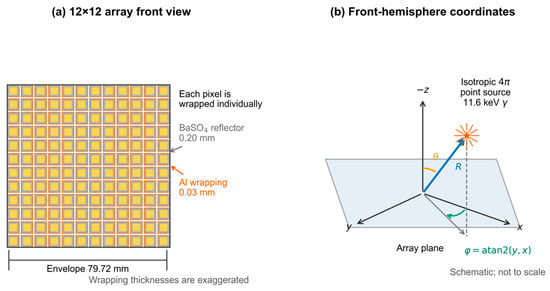
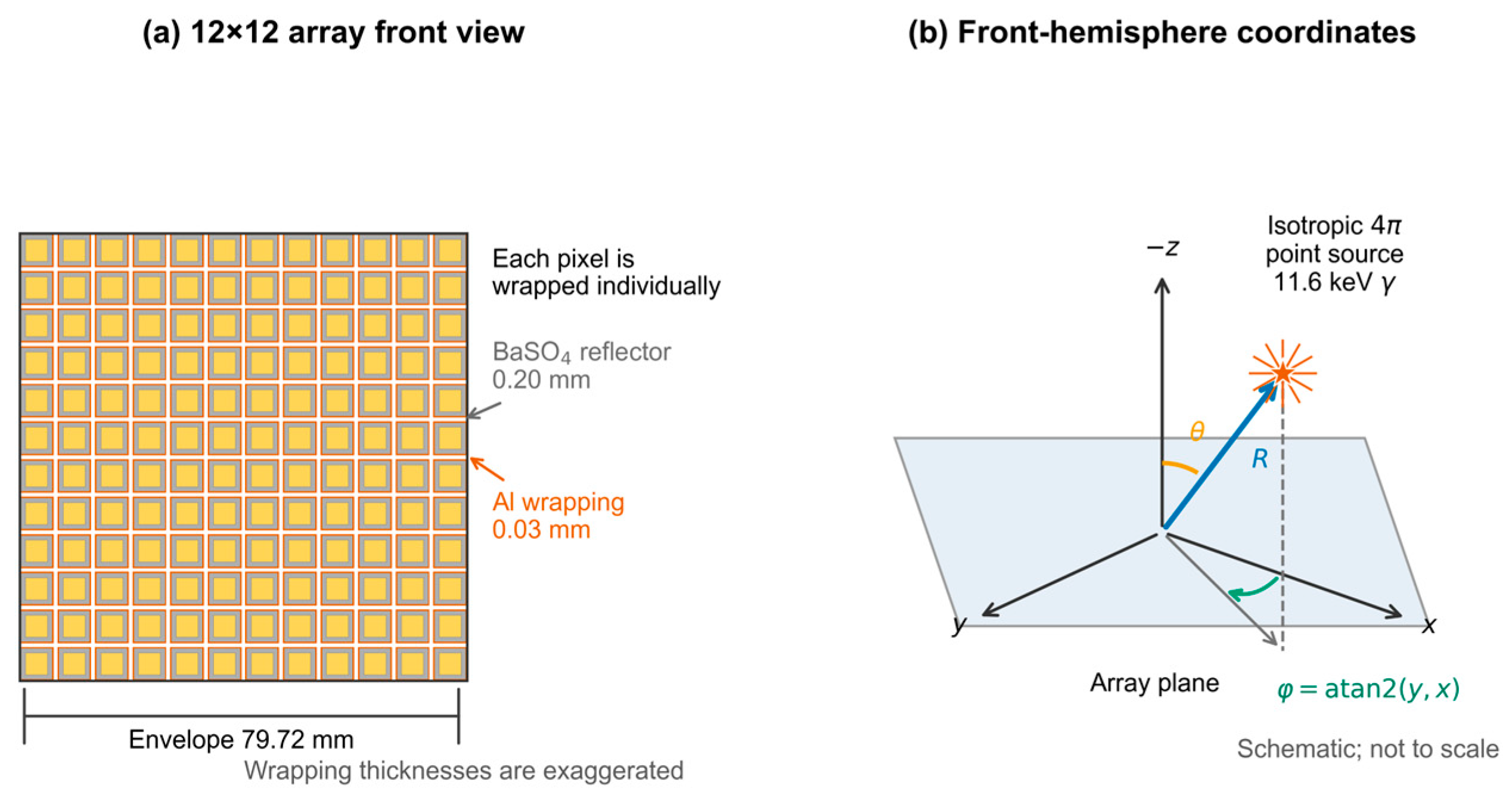
Figure 1 presents the detector geometry and front-hemisphere coordinate system. Figure 1a shows the independently wrapped 12 × 12 pixel array, and Figure 1b defines the point-source position through R, θ, and φ.
Figure 1.
Geometry and coordinate definition of the 12 × 12 YSO pixelated scintillator array: (a) front view of the array; (b) front-hemisphere coordinate system, where θ is measured from the entrance-face normal (−z) and φ from +x to the in-plane projection ρ of the source vector R.
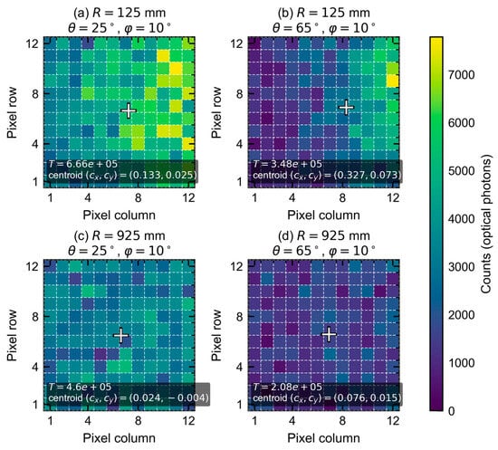
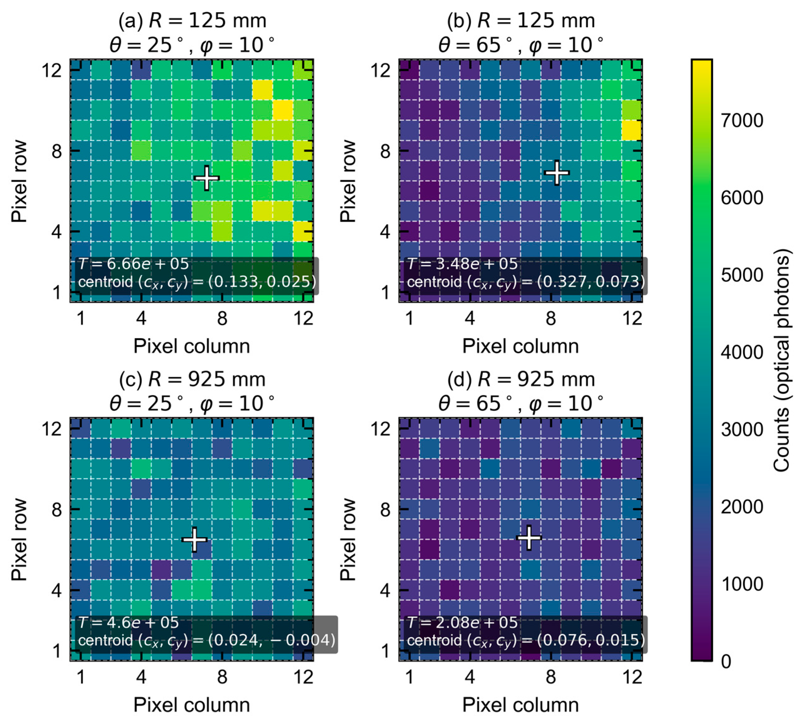
Figure 2 shows four representative response heatmaps at φ = 10°, with R = 125 or 925 mm and θ = 25° or 65°. Both distance and polar angle change the total response, hotspot pattern, and centroid, supporting the joint use of absolute response rate and two-dimensional shape to estimate direction and distance.
Figure 2.
Response maps at R = 125 or 925 mm, θ = 25° or 65°, and φ = 10°. The shared scale gives unique optical-interface counts; crosses indicate count-weighted centroids. Emitted exposures are 0.2 million primaries in (a,b) and 9.6 million in (c,d).
2.3. Physical Basis of Angular Sensitivity
The array obtains directional sensitivity from changes in its spatial response with viewing direction. Geometric projection and the finite array solid angle redistribute irradiation among pixels. At 11.6 keV, unequal air paths to the near and far sides amplify count contrast at oblique incidence, while attenuation reduces the total response. Independent wrapping preserves this spatial contrast. In the 224-position multi-distance scan, each of the 624,641 responding primary events produced an interface response within one pixel. Response centroids summarize the displacement of the pattern, while its higher-order spatial structure supplies additional directional information.
The same mechanisms limit performance close to the entrance-face normal. As θ approaches 0°, directional pattern differences and centroid displacement diminish, and the response becomes more nearly centrosymmetric. Azimuthal information therefore weakens, making near-normal azimuth estimation less reliable than estimation at larger polar angles. Section 4.2 relates this limitation to the simulated error distribution.
2.4. Data Generation and Quality Control
Each physical source position supplied an accumulated 12 × 12 response matrix, its emitted-primary count, and source coordinates. Zero-response primaries were included in . The 224-position multi-distance scan contained 810,800,000 emitted primaries, 624,641 responding events, and 97,678,686 unique interface-photon counts, equivalent to 156.4 counts per responding primary. Optical photons from one primary share an interaction history, and the physical source position was used as the statistical unit for comparisons across geometry.
Each response was linked to its source coordinates, emitted exposure, CLHEP seeds, initialized material settings, and input and model-checkpoint identifiers. Quality checks covered event counts, all 144 pixel totals, coordinates, and split membership. The 458 base responses and 1406 exposure prefixes were reconstructed from sparse primary-event histories. A prefix with exposure N accumulated events with IDs from 0 through N − 1, including zero-response primaries in the exposure denominator.
2.5. Scan Design and Dataset Partitioning
The response library combined a 234-position angular scan at R = 300 mm with a 224-position multi-distance scan. Each fixed-distance position used 1 million primary photons. Its 192 training positions covered θ = 10–80° in 10° increments and φ = 0–345° in 15° increments; 24 validation positions used θ = 15°, 35°, 55°, or 75° and six staggered azimuths. The remaining eighteen positions provided fixed-distance diagnostics. These responses supplied denser angular coverage for the joint model and were combined with the multi-distance responses using one physical position per sample.
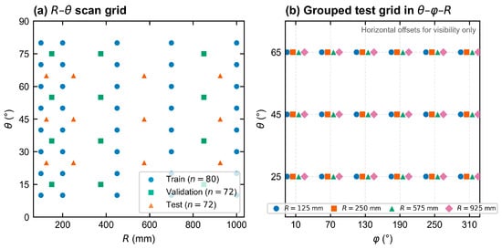
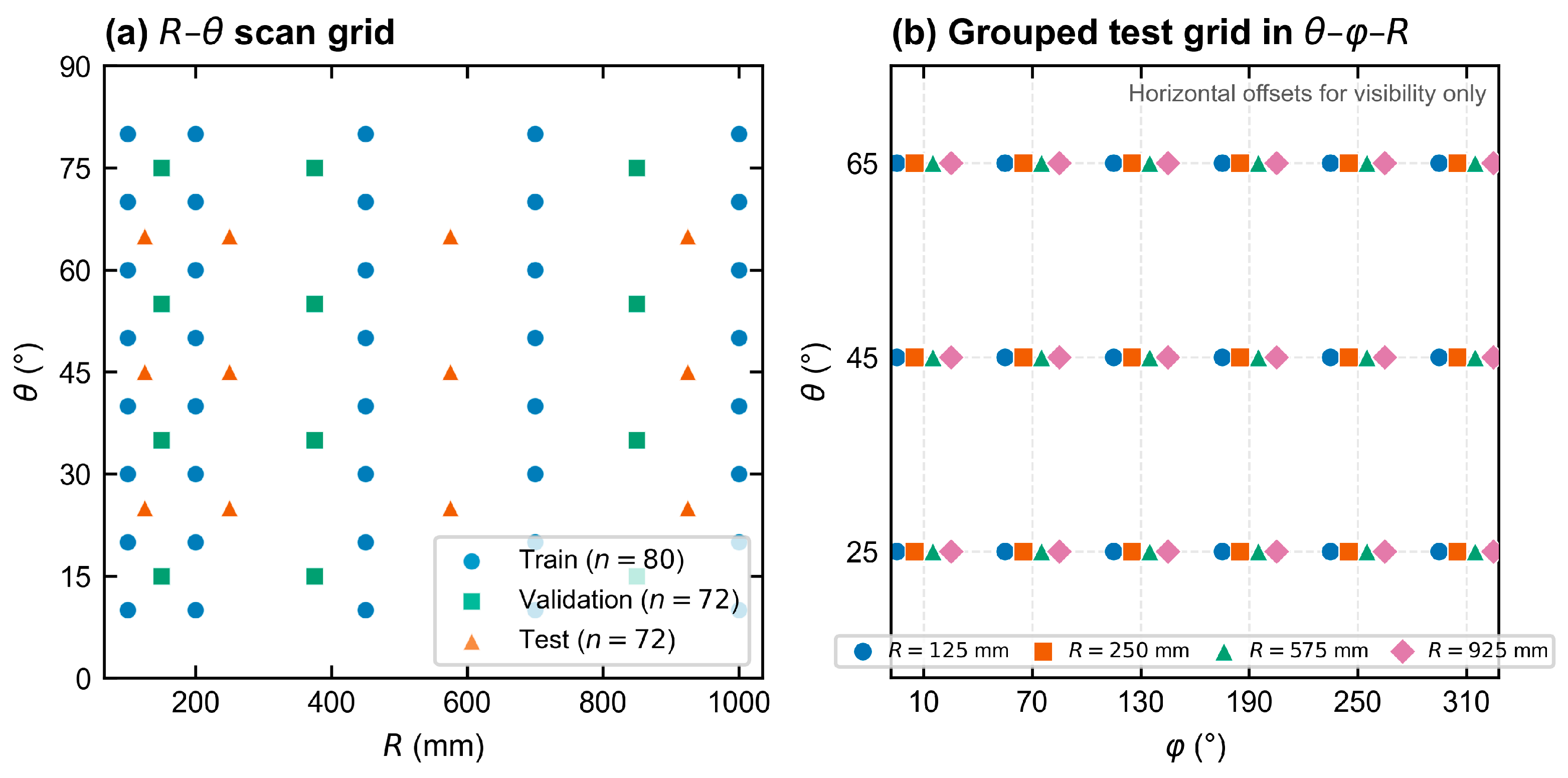
The multi-distance scan comprised 80 training, 72 validation, and 72 evaluation positions on staggered distance and angular grids specified in Table 2 and Figure 3. Combining both scans gave 272 training, 96 validation, 72 multi-distance evaluation, and 18 fixed-distance diagnostic positions.
Table 2.
Multi-distance scan design.
Figure 3.
Multi-distance scan grids: (a) staggered training/validation/evaluation positions in R–θ; (b) the 72 evaluation positions in θ–φ–R. This scan contains 80/72/72 positions. Adding the fixed-300 mm scan gives 272 training, 96 validation, and 72 multi-distance evaluation positions, with 18 fixed-distance diagnostics reported separately.
For the multi-distance library, emitted exposure increased approximately with to compensate for the geometric dilution of a point-source response. The allocation in Equation (7) uses 1 million primaries at 300 mm as its reference, a minimum of 0.2 million primaries, and upward rounding in increments of 0.1 million:
Here, M denotes one million emitted primaries. Additional simulations used 4 million primaries per realization at 300 random positions, 100 calibration positions, 12 positions with 10 independent histories each, and 24 stress positions. Random positions were sampled uniformly in R from 100 to 1000 mm, uniformly in cosθ between cos80° and cos10°, and uniformly in φ from 0° to 360°. Responses at 1 and 2 million primaries were nested prefixes of each 4-million-primary history.
2.6. Dual-Branch CNN with Spatial–Global Feature Fusion
The model combines two descriptions of the detector response. The spatial branch reads the relative count pattern and pixel coordinates, while the global branch receives response rate and spatial summary measures. Let denote the count in pixel (i, j), and let T denote the total response. The normalized spatial probability was
The spatial branch received a 3 × 12 × 12 tensor, with its first channel given by the square-root transformation
and the other two channels were fixed x- and y-coordinate grids. This representation separates relative shape from total amplitude while retaining where each feature lies on the array. The global branch receives the rate and spatial summaries in the six-dimensional vector
The six descriptors were , , , , , and . Pixel centers were mapped linearly to −1 through 1 on each axis, with as the weights. Each centroid coordinate is the corresponding weighted mean; each spread is the square root of the weighted mean squared displacement from that centroid; covariance is the weighted mean product of the two displacements. supplied the rate denominator. The inputs therefore combined normalized shape with response per emitted primary.
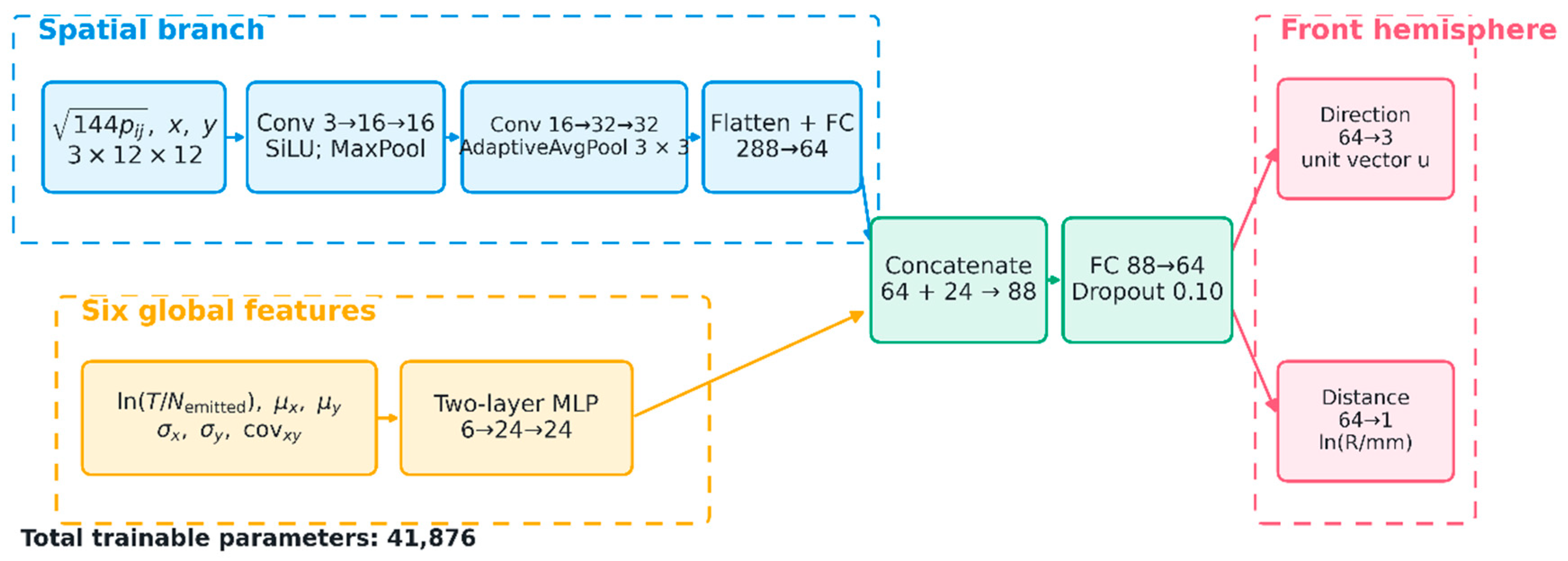
Convolutional layers extract local patterns across neighboring pixels, while pooling summarizes them into a smaller representation. The spatial branch used Conv 3 → 16 → 16, 2 × 2 max pooling, Conv 16 → 32 → 32, and adaptive average pooling to 3 × 3, followed by Linear 288 → 64. The global branch used Linear 6 → 24 → 24. Their 64 and 24 features were combined through Linear 88 → 64, SiLU, and dropout 0.10, followed by separate direction and distance heads. Full contained 41,876 parameters. Raw direction outputs were mapped to and normalized as , yielding a unit vector in the front hemisphere. For distance logit b, and , with R expressed in millimeters. The distance output was thus bounded between 100 and 1000 mm.
The direction target was the unit vector
The unit-vector target provides a continuous representation across the 0°/360° azimuth boundary [25,26]. Training minimized the batch mean of with unit coefficients. The direction term was . The polar-angle and log-distance terms were Smooth-L1 losses with β = 0.05, applied to and , respectively; angles in the polar residual were in radians. The azimuth term compared transverse directions using , where and . It was averaged over targets with θ > 1°. AdamW [27] used a learning rate of 0.002, weight decay , batch size 32, a maximum of 500 epochs, and early-stopping patience of 100 epochs. Epoch selection minimized validation θ MAE/90 + circular φ MAE/180 + mean absolute log-distance error.
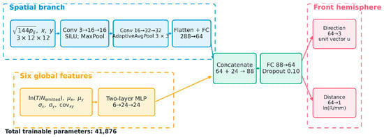
Figure 4 summarizes the architecture. The upper path is the CNN spatial branch, the lower path is the six-feature multilayer perceptron (MLP), and the fused representation feeds the direction and distance heads.
Figure 4.
Spatial–global dual-branch CNN. The normalized pixel pattern and coordinate channels supply 64 spatial features; six global descriptors supply 24 features. Their combination feeds direction-vector and log-distance heads. CNN denotes convolutional neural network, Conv convolution, MLP multilayer perceptron, and FC fully connected layer. The model contains 41,876 parameters; Section 2.6 specifies its output mappings.
2.7. Training Procedure
Full and the input-matched MLP used training seeds 2026, 2027, and 2028, distance-balanced physical-position sampling, and C4 rotations. Their sampling and rotation schedules were matched, with separate random streams and two CPU threads. Single-run figures used seed 2026, while model comparisons summarized all three seeds. Primary performance metrics used single-view predictions; postprocessing was assessed separately as described in Section 2.8.
Training used 400 response candidates at 272 physical positions. At 48 positions with R = 450, 700, or 1000 mm, sufficiently long histories supplied additional exact exposure prefixes. Distance-balanced sampling allocated approximately 36% of planned training visits to these prefixes. Candidates from the same history shared events. Epoch selection used the 96 validation responses, and Supplementary Material S1 provides the exposure coverage and model identities.
2.8. Comparison Methods and Postprocessing
The input-matched MLP received the 144 flattened spatial values defined in Equation (9) and the same six global descriptors. It contained 44,356 parameters and used the same output mappings, loss, physical splits, response candidates, sampling, rotations, and validation selection as Full. A forward-response inverse estimator used per-emission first and second pixel-response moments, including zero-response events, from the 272 training positions. Kernel interpolation in direction and log-distance, with geometric scaling, supplied the expected response and covariance. Inversion minimized a Gaussian negative log-likelihood after projection onto ten fixed spatial polynomial components. Twelve candidate settings were compared on the 96 validation positions.
Random Forest [28], Extra Trees [29], template/kNN [30], and a Global-only neural model provided additional comparisons on the same 72-position response matrices. The tree and Global-only models received six global descriptors; template/kNN used spatial response and normalized rate. Global-only contained 2628 parameters and used base training responses without rotation augmentation. Full and MLP-150 shared the additional exposure candidates and augmentation, providing a matched comparison of spatial representations.
Postprocessing was evaluated using four-view test-time augmentation (TTA), centroid azimuth, and centroid fusion. TTA rotated each response matrix through four right-angle views, recomputed the spatial and global inputs, and transformed predicted directions back to the original frame. The four direction vectors were averaged and normalized, and distance was obtained by exponentiating the mean predicted log-distance. A resultant norm below triggered a fallback to the unrotated direction.
The centroid estimator used . Fusion assigned the centroid azimuth to the Full prediction while preserving its polar angle and distance, equivalent to a fixed centroid weight of 1. The centroid method supplied azimuth only. Postprocessing metrics were calculated on the same 72-position multi-distance grid and exposure schedule as the primary Full analysis.
2.9. Evaluation Metrics and Statistical Analysis
Performance was summarized by polar absolute error, shortest circular azimuth error, three-dimensional angular separation, distance absolute error, and distance MAPE. Each MAE assigned equal weight to physical source positions. Distribution summaries included medians, P90, P95, P99, maxima, and the fractions with directional errors above 15°, 30°, and 60°. Circular azimuth error was defined as [31]
Three-seed summaries report the mean and sample SD of metrics computed separately for each training seed. For paired Full–MLP comparisons, seed-level errors were averaged within each position before 5000 position-bootstrap resamples supplied exploratory 95% intervals conditional on the fitted models. These intervals exclude development-selection uncertainty and multiplicity adjustment. Fixed-weight Monte Carlo variation was evaluated using ten independent histories at each of twelve positions, with nested exposures within a history. The multi-distance and random-position responses were inspected during model development and were therefore analyzed as development evaluation sets.
3. Results
3.1. Performance on the Multi-Distance Evaluation Grid
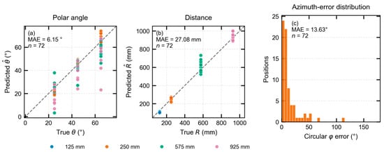
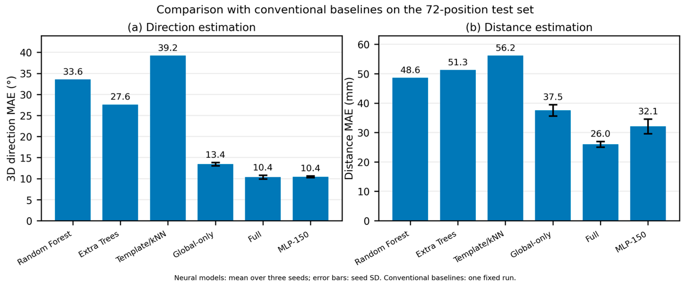
Across three seeds, Full achieved directional and distance MAEs of 10.4 ± 0.5° and 26.0 ± 0.9 mm on the 72-position multi-distance grid (Table 3).
Table 3.
Neural-model performance on the 72-position multi-distance grid, mean ± sample SD across seeds 2026–2028. Full and MLP-150 share the training-response candidates; Global-only uses base responses and six descriptors.
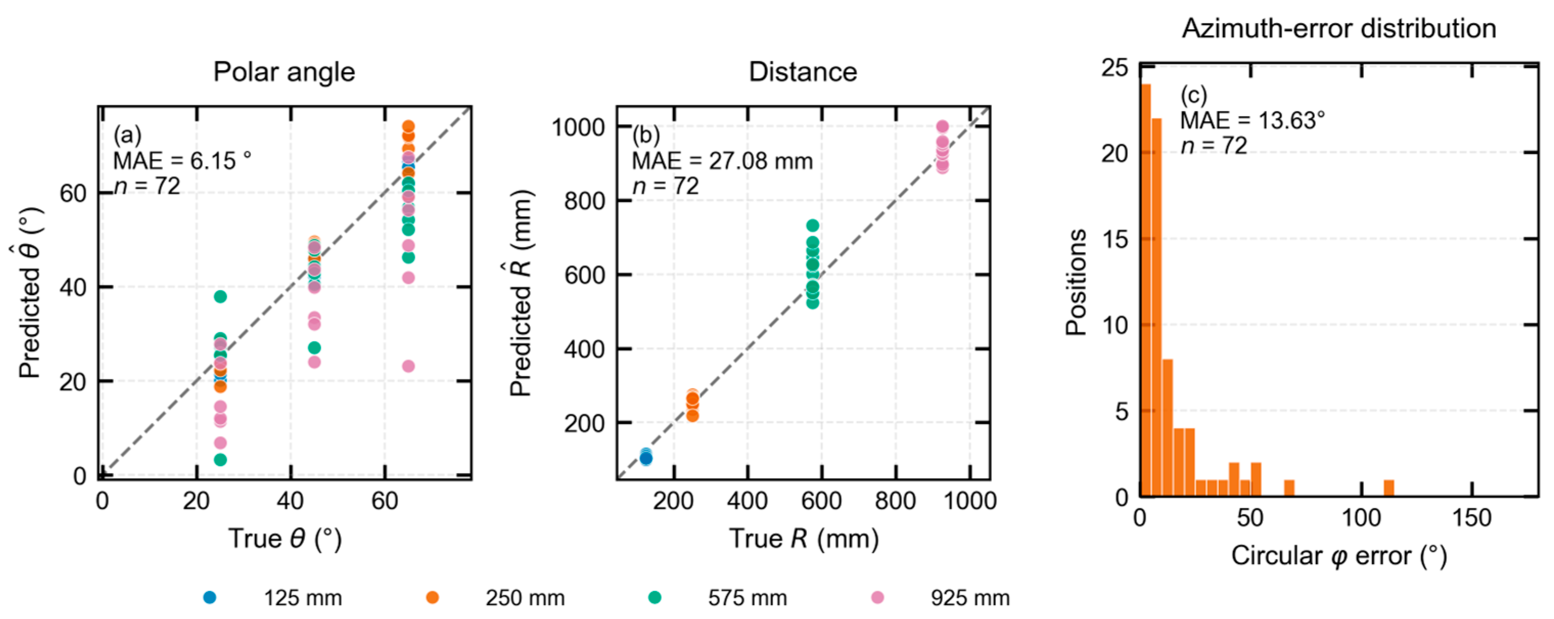
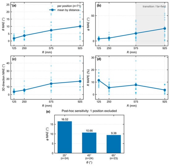
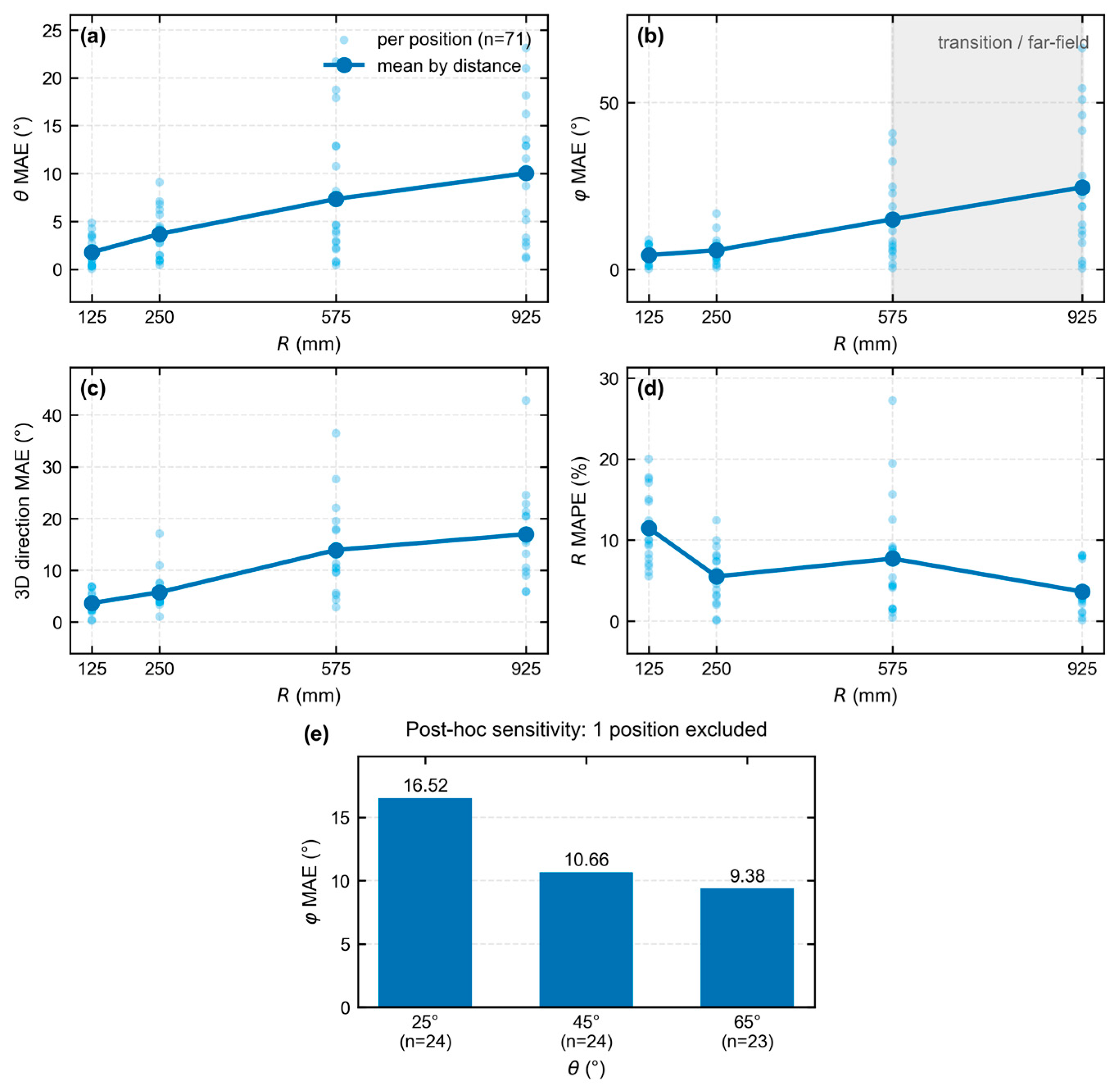
Figure 5 and Figure 6 show the predictions and geometric dependence of errors. Across the 71 positions in Figure 6, angular errors increased with distance, while circular-azimuth MAE decreased with polar angle. The separate R = 300 mm diagnostics gave mean directional and distance MAEs of 6.6° and 11.7 mm.
Figure 5.
Full seed-2026 predictions on the 72-position multi-distance grid: (a) polar angle; (b) distance; (c) circular-azimuth-error histogram. Colors indicate source distance, and dashed lines indicate equality. Each distance contains eighteen positions, with emitted exposures of 0.2/0.7/3.7/9.6 million primaries at 125/250/575/925 mm.
Figure 6.
Full seed-2026 errors for 71 source positions in the sensitivity analysis: (a) polar absolute error; (b) circular-azimuth absolute error; (c) three-dimensional direction error; (d) distance relative error, with the mean expressed as MAPE; (e) circular-azimuth MAE by true polar angle. Light points represent individual positions. Upper-panel means use eighteen positions each at 125, 250, and 575 mm and seventeen at 925 mm. Bottom bars summarize 24, 24, and 23 positions at 25°, 45°, and 65°, respectively.
3.2. Neural Models and Fixed-Exposure Results
On the multi-distance grid, Full and MLP-150 each achieved a mean directional MAE of 10.4°, with distance MAEs of 26.0 and 32.1 mm (Table 3). Both models improved on Global-only; the difference between Full and MLP-150 was more evident in distance.
Errors decreased with increasing exposure at the 300 random positions (Table 4). At 4 million primaries, Full achieved directional and distance MAEs of 15.6° and 52.6 mm, compared with 16.7° and 55.2 mm for the input-matched MLP. Equal emitted exposure exposed larger errors at low-response locations.
Table 4.
Fixed-exposure results on the same 300 random positions. Neural entries are mean ± sample SD across three training seeds; the physical inverse uses one fixed implementation. Exposure is the number of emitted primaries per position. P95 denotes the 95th percentile of errors across source positions.
Paired position-bootstrap analyses provided exploratory 95% confidence intervals for the Full–MLP differences at all three exposures. Directional intervals favored Full; at 4 million primaries, the mean Full-minus-MLP difference was −1.2°, with an interval of [−2.1, −0.3]°. Distance intervals indicated less clear separation (Supplementary Material S1).
3.3. Comparison with Input-Matched and Physical Baselines
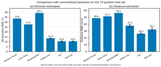
Figure 7 compares the estimators on the multi-distance grid, where Full and MLP-150 gave lower mean errors. The physical inverse estimator also had larger mean errors than Full at the fixed-exposure random positions (Table 4; Supplementary Material S1).
Figure 7.
Direction and distance MAEs on the 72-position response matrices. Neural bars represent three-seed means with between-training-seed sample SD; conventional methods use one fixed run. Global-only uses six descriptors, and MLP-150 uses the 144 spatial values and those descriptors. Full and MLP-150 share exposure-prefix training candidates, while the other methods use base training responses.
Full had lower directional error at more than half of the random positions at each exposure. Distance benefits were less uniform and, at the lowest exposure, concentrated in a minority of positions.
The far-field, near-axis stress set reversed the ordering between Full and the physical inverse estimator. At 4 million primaries, the inverse estimator achieved direction/distance MAEs of 19.2°/32.2 mm, compared with 23.7°/68.7 mm for Full. Comparative performance therefore depended on the sampled geometry.
3.4. Spatial Error Patterns and Variation Among Training Runs
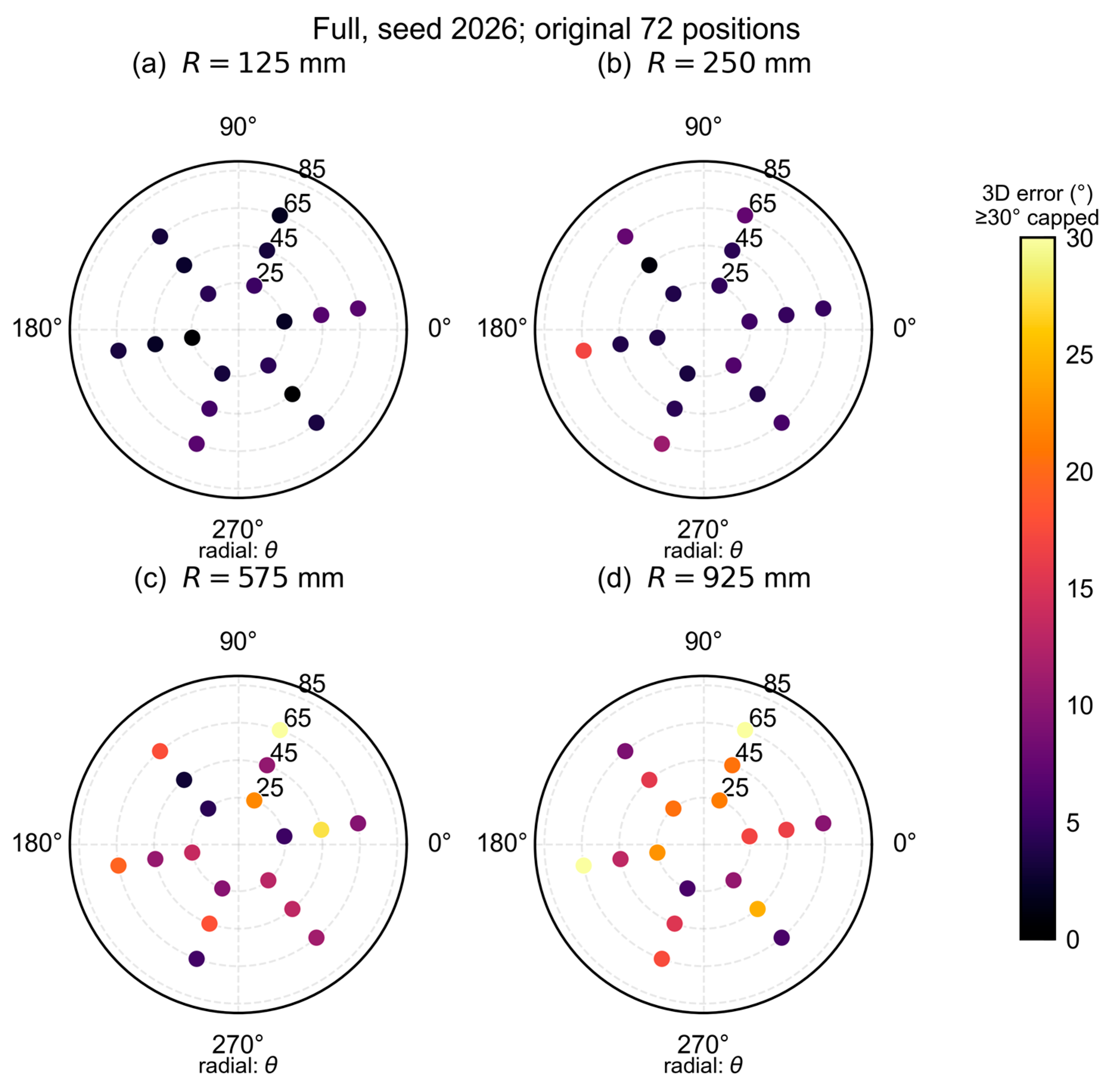
Training-seed variation was smaller than the spread of errors across positions (Table 4). Error distributions had substantial upper tails: for Full seed 2026 at 1 million primaries, the directional median was 16.8° and P95 was 68.7°.
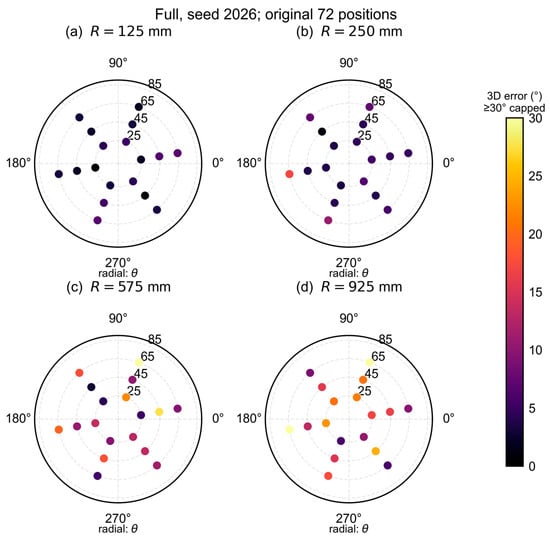
Figure 8 maps large directional errors in difficult viewing geometries. Some random positions retained large errors at 4 million primaries. Supplementary Material S1 provides uncapped errors and distribution summaries.
Figure 8.
Polar maps of Full seed-2026 three-dimensional direction errors at four distances: (a) R = 125 mm; (b) R = 250 mm; (c) R = 575 mm; and (d) R = 925 mm. Angular and radial coordinates represent the true azimuth φ and polar angle θ, respectively. Each panel contains eighteen source positions. The shared color scale is capped at 30°, affecting 3 of 72 positions; the actual maximum is 75.7°. Uncapped errors are supplied with the numerical data.
3.5. Exposure Sensitivity and Monte Carlo Repetitions
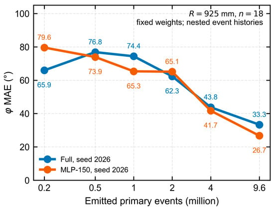
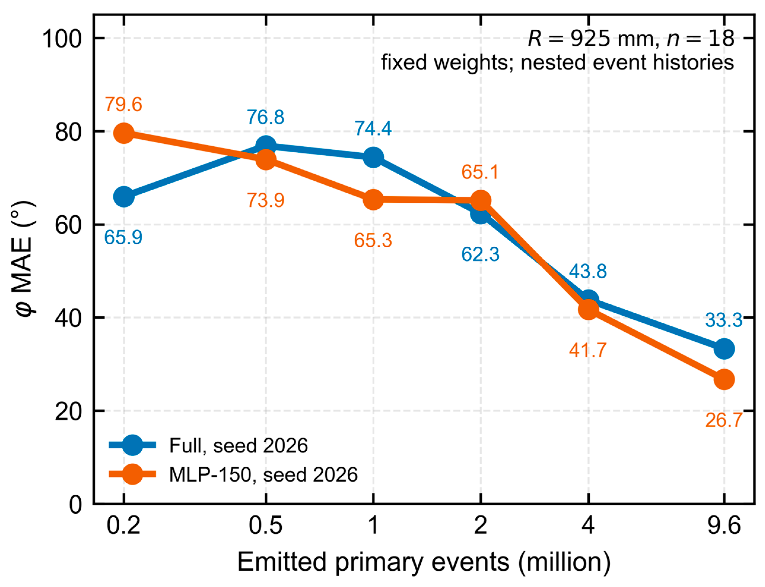
Figure 9 shows circular-azimuth MAE across an exposure series at eighteen R = 925 mm positions using fixed Full and MLP-150 seed-2026 weights. Full’s initial increase in error is consistent with prediction instability under limited response counts. Both models improved overall with exposure, while their relative accuracy varied across exposure levels.
Figure 9.
Circular-azimuth MAE versus emitted exposure at eighteen R = 925 mm positions. Full and MLP-150 use fixed seed-2026 weights and identical responses at each exposure. The horizontal axis is logarithmic. Responses at 0.2/0.5/1/2/4 million primaries are nested event prefixes, with the complete 9.6-million history as the endpoint.
Ten independent Monte Carlo histories at each of twelve positions showed reduced variation with increasing exposure at fixed model weights. For Full seed 2026, the average within-position distance sample SD decreased from 54.2 to 23.9 mm between 1 and 4 million primaries; angular variation also decreased (Supplementary Material S1).
3.6. Postprocessing of Azimuth Predictions
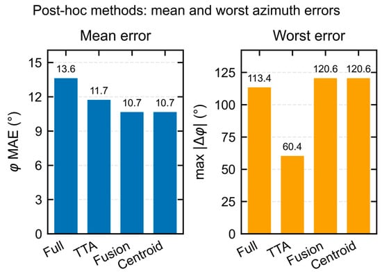
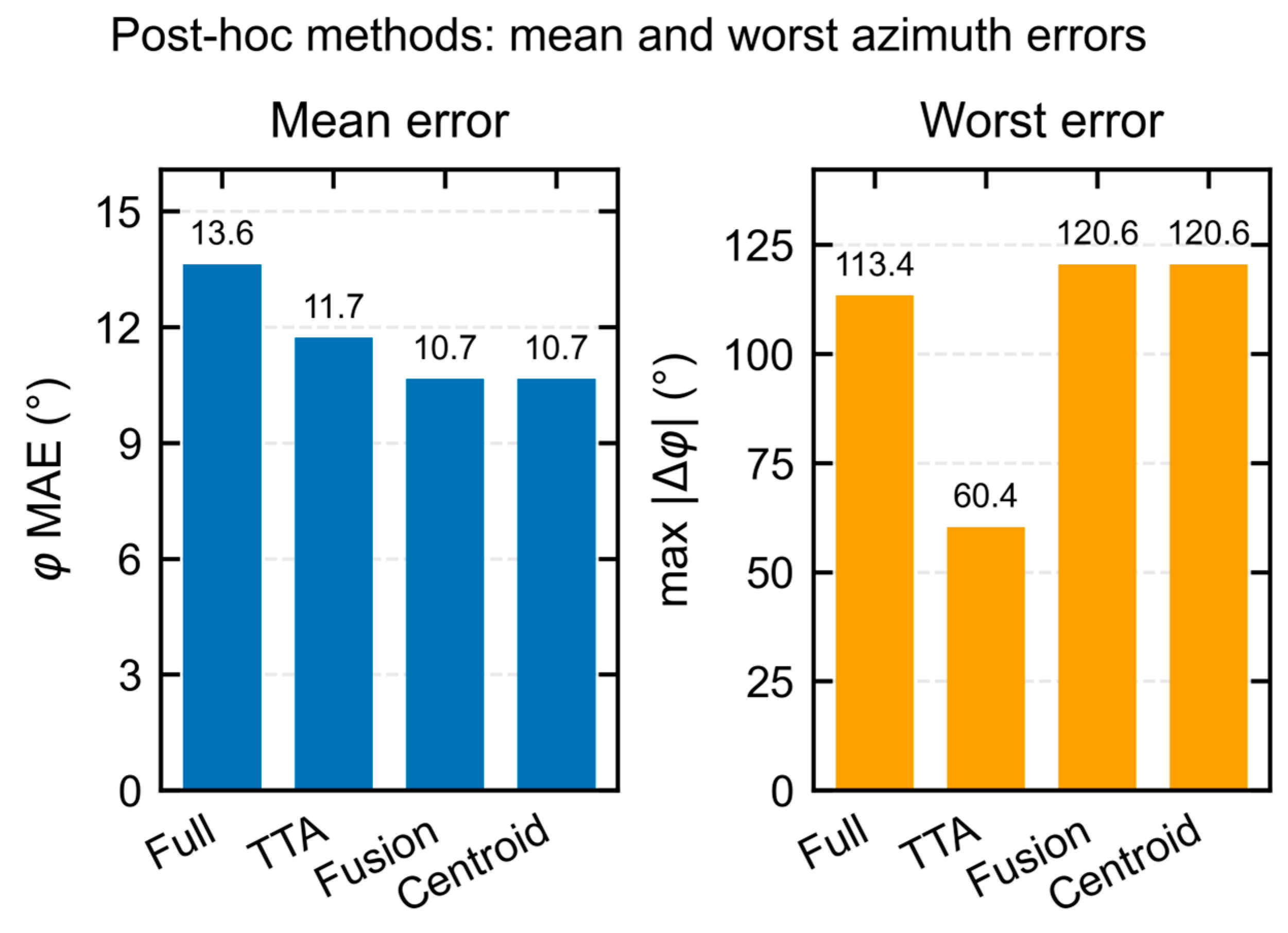
Figure 10 shows that TTA reduced mean and maximum azimuth error; the maximum fell from 113.4° to 60.4°. Centroid-based postprocessing gave a lower mean with a larger maximum. Centroid and Fusion coincided because the centroid weight was 1.
Figure 10.
Postprocessing of Full seed-2026 predictions on the 72-position multi-distance grid: (left) mean circular-azimuth error; (right) maximum circular-azimuth error. TTA averages four rotation-corrected views. Fusion uses centroid azimuth with Full polar angle and distance; its fixed centroid weight of 1 gives the same azimuth results as Centroid. All methods use the same response matrices and emitted exposures.
4. Discussion
4.1. Spatial and Global Information in Joint Localization
Full combines normalized spatial patterns with response per emitted primary and low-order spatial moments. On the multi-distance grid, its mean directional error was similar to that of the input-matched MLP, while its distance error was lower. Fixed-exposure random-position comparisons also favored Full in mean direction, with smaller differences in distance. Together, these findings support the use of spatial structure alongside rate information for the simulated localization task.
Performance across the comparison methods varied with the evaluation geometry. Conventional estimators using fewer descriptors were less accurate on the multi-distance grid, whereas the forward-response inverse estimator performed better in the far-field, near-axis stress set. Learned regression and forward-response interpolation therefore offered different strengths. The matched Full–MLP comparison provides evidence about spatial representation, while the broader comparisons describe the behavior of estimators with different input access and training responses.
Exposure prefixes broadened the training responses at 48 coordinates, while validation used distance-adaptive base responses. Normalizing a count matrix preserves spatial proportions and retains the fluctuations associated with its acquisition exposure. For similar segmented arrays, joint localization should therefore be assessed across viewing geometries using both spatial patterns and response rate under matched emitted exposures.
4.2. Exposure Dependence and Geometric Ambiguity
Near the entrance-face normal, response patterns become more nearly centrosymmetric and transverse directional information weakens. Count fluctuations can then produce large azimuth changes even when the three-dimensional directional change is smaller. The decrease in azimuth MAE with polar angle in Figure 6 is consistent with this geometric dependence. At low exposure, the limited number of responding primaries makes spatial response proportions and global descriptors more sensitive to event-count fluctuations. The fixed nonlinear mapping can amplify these input variations, producing unstable azimuth predictions and the non-monotonic behavior observed for Full in Figure 9. Increasing exposure better samples the response pattern and supports the overall reduction in error. Because optical photons from one primary share an interaction history, the primary-event count governs independent sampling of the response.
The distance-dependent allocation compensated for approximate geometric dilution during response-library construction. Fixed exposures of 1, 2, and 4 million primaries provided a complementary evaluation across distance. At each level, every position had the same known emitted exposure, while the number of responding events varied with geometry and attenuation. The random-position sample characterized performance across the sampled domain, and the stress set concentrated on difficult far-field, near-axis conditions.
Distance inference is conditional on known emitted exposure, determined by source activity, acquisition time, and line-emission probability. Unknown source strength requires an additional measurement or prior constraint to separate activity from distance.
4.3. Limitations and the Simulation-to-Experiment Gap
The optical-response model uses effective surface properties and interface counts, with SiPM response, electronics, and background requiring detector-specific characterization [23,24]. Transfer to hardware will require optical calibration and physical-source measurements; domain randomization [32] could broaden the training conditions.
The simulated domain comprises one isotropic 11.6 keV point source. Extension to other energies or source configurations, together with independent evaluation and uncertainty calibration, remains future work.
5. Conclusions
A Geant4 response model and a spatial–global dual-branch CNN were used for joint direction and distance estimation conditional on known emitted exposure. Full achieved three-seed mean directional and distance MAEs of 10.4° and 26.0 mm on the 72-position multi-distance grid. Same-coordinate exposure controls and spatial error maps showed how counting statistics and viewing geometry influence performance.
The combined spatial and rate representation provides useful localization information under the simulated conditions. Performance depends on exposure and viewing geometry, and the physical inverse estimator performed better in the stress region. Postprocessing improved mean azimuth accuracy, with different effects on maximum error. Further evaluation and detector measurements will establish the scope for experimental use.
Supplementary Materials
The following supporting information can be downloaded at: https://www.mdpi.com/article/10.3390/app162110846/s1, Supplementary Material S1 provides initialized optical and transport settings, event-count checks, exposure and training definitions, model comparisons, random-position and stress results, paired intervals, error distributions, and fixed-weight Monte Carlo variation. The accompanying numerical archive contains model identities, configuration records, implementation files, and supporting data.
Author Contributions
Software, Y.L.; algorithm code development and review, X.Z.; simulation, Q.L.; writing—original draft preparation, Y.L.; supervision, J.Z. and Y.Y.; methodology and supervision, Q.D. All authors have read and agreed to the published version of the manuscript.
Funding
This research received no external funding.
Institutional Review Board Statement
Not applicable. This study was based entirely on simulation and did not involve humans, animals, or clinical data.
Informed Consent Statement
Not applicable.
Data Availability Statement
Numerical outputs, initialized configuration records, and implementation files are provided in the accompanying Supplementary archive. The complete transport histories and larger production datasets are available from the corresponding author upon reasonable request.
Conflicts of Interest
The authors declare no conflicts of interest.
Abbreviations
| Abbreviation | Definition |
| CNN | Convolutional neural network |
| ESR | Enhanced specular reflector |
| MAE | Mean absolute error |
| MAPE | Mean absolute percentage error |
| MLP | Multilayer perceptron |
| P95 | 95th percentile |
| SiPM | Silicon photomultiplier |
| TTA | Test-time augmentation |
| YSO(Ce) | Cerium-doped yttrium orthosilicate |
References
- Zhao, Q.; Wang, Z.; Li, L.; Li, X.; Zhao, C.; Zhao, M.; Li, F.; Cheng, M.; Zhu, B.; Zhou, R.; et al. A two-dimensional array detector for determining the direction to gamma-ray source. Nucl. Instrum. Methods Phys. Res. A 2022, 1040, 166985. [Google Scholar] [CrossRef] [Scilit]
- Vetter, K.; Barnowski, R.; Haefner, A.; Joshi, T.H.Y.; Pavlovsky, R.; Quiter, B.J. Gamma-ray imaging for nuclear security and safety: Towards 3-D gamma-ray vision. Nucl. Instrum. Methods Phys. Res. A 2018, 878, 159–168. [Google Scholar] [CrossRef] [Scilit]
- Al Hamrashdi, H.; Monk, S.D.; Cheneler, D. Passive gamma-ray and neutron imaging systems for national security and nuclear non-proliferation in controlled and uncontrolled detection areas: Review of past and current status. Sensors 2019, 19, 2638. [Google Scholar] [CrossRef] [Scilit] [PubMed]
- Hellfeld, D.; Bandstra, M.S.; Vavrek, J.R.; Gunter, D.L.; Curtis, J.C.; Salathe, M.; Pavlovsky, R.; Negut, V.; Barton, P.J.; Cates, J.W.; et al. Free-moving quantitative gamma-ray imaging. Sci. Rep. 2021, 11, 20515. [Google Scholar] [CrossRef] [Scilit] [PubMed]
- Haefner, A.; Barnowski, R.; Luke, P.; Amman, M.; Vetter, K. Handheld real-time volumetric 3-D gamma-ray imaging. Nucl. Instrum. Methods Phys. Res. A 2017, 857, 42–49. [Google Scholar] [CrossRef] [Scilit]
- Hellfeld, D.; Barton, P.; Gunter, D.; Haefner, A.; Mihailescu, L.; Vetter, K. Real-time free-moving active coded mask 3D gamma-ray imaging. IEEE Trans. Nucl. Sci. 2019, 66, 2252–2260. [Google Scholar] [CrossRef] [Scilit]
- Shi, R.; Chen, Y.; Dang, X.; Wei, M. Experimental evaluation of reconstruction algorithms for scintillation crystal array based on charge projection readout. Nucl. Instrum. Methods Phys. Res. A 2019, 937, 117–124. [Google Scholar] [CrossRef] [Scilit]
- Lerche, C.W.; Salomon, A.; Goldschmidt, B.; Lodomez, S.; Weissler, B.; Solf, T. Maximum likelihood positioning and energy correction for scintillation detectors. Phys. Med. Biol. 2016, 61, 1650–1676. [Google Scholar] [CrossRef] [Scilit] [PubMed]
- Lavelle, C.M.; Miller, E.C.; Ribaudo, C.; Drenkow, N.; Sivels, C.; Mattson, J. Directional pixelated gamma-ray spectrometer utilizing convolutional neural network and simulated training data. IEEE Trans. Nucl. Sci. 2025, 72, 1602–1611. [Google Scholar] [CrossRef] [Scilit]
- Daniel, G.; Ceraudo, F.; Limousin, O.; Maier, D.; Meuris, A. Automatic and real-time identification of radionuclides in gamma-ray spectra: A new method based on a convolutional neural network trained with a synthetic data set. IEEE Trans. Nucl. Sci. 2020, 67, 644–653. [Google Scholar] [CrossRef] [Scilit]
- Bilton, K.J.; Joshi, T.H.Y.; Bandstra, M.S.; Curtis, J.C.; Hellfeld, D.; Vetter, K. Neural network approaches for mobile spectroscopic gamma-ray source detection. J. Nucl. Eng. 2021, 2, 190–206. [Google Scholar] [CrossRef] [Scilit]
- Durbin, M.; Sheatsley, R.; McDaniel, P.; Lintereur, A. Experimental tests of Gamma-ray Localization Aided with Machine-learning (GLAM) capabilities. Nucl. Instrum. Methods Phys. Res. A 2022, 1038, 166905. [Google Scholar] [CrossRef] [Scilit]
- Chechev, V.P. 238Pu. In Table de Radionucléides; LNE–LNHB/CEA. 2010. Available online: https://www.lnhb.fr/nuclides/Pu-238_tables.pdf (accessed on 17 October 2026).
- Basaglia, T.; Bell, Z.W.; D’Agostino, D.; Dressendorfer, P.V.; Giani, S.; Pia, M.G.; Saracco, P. Geant4: A game changer in high energy physics and related applicative fields. Future Gener. Comput. Syst. 2024, 159, 411–422. [Google Scholar] [CrossRef] [Scilit]
- Allison, J.; Amako, K.; Apostolakis, J.; Arce, P.; Asai, M.; Aso, T.; Bagli, E.; Bagulya, A.; Banerjee, S.; Barrand, G.; et al. Recent developments in Geant4. Nucl. Instrum. Methods Phys. Res. A 2016, 835, 186–225. [Google Scholar] [CrossRef] [Scilit]
- Dietz-Laursonn, E. Peculiarities in the simulation of optical physics with Geant4. arXiv 2016, arXiv:1612.05162. [Google Scholar] [CrossRef] [Scilit]
- Chewpraditkul, W.; Wanarak, C.; Szczesniak, T.; Moszynski, M.; Jary, V.; Beitlerova, A.; Nikl, M. Comparison of absorption, luminescence and scintillation characteristics in Lu1.95Y0.05SiO5:Ce,Ca and Y2SiO5:Ce scintillators. Opt. Mater. 2013, 35, 1679–1684. [Google Scholar] [CrossRef] [Scilit]
- Knoll, G.F. Radiation Detection and Measurement, 4th ed.; John Wiley & Sons: Hoboken, NJ, USA, 2010. [Google Scholar]
- Nikl, M. Scintillation detectors for X-rays. Meas. Sci. Technol. 2006, 17, R37–R54. [Google Scholar] [CrossRef] [Scilit]
- Dujardin, C.; Auffray, E.; Bourret-Courchesne, E.; Dorenbos, P.; Lecoq, P.; Nikl, M.; Vasil’ev, A.N.; Yoshikawa, A.; Zhu, R.-Y. Needs, trends, and advances in inorganic scintillators. IEEE Trans. Nucl. Sci. 2018, 65, 1977–1997. [Google Scholar] [CrossRef] [Scilit]
- van Eijk, C.W.E. Inorganic scintillators in medical imaging. Phys. Med. Biol. 2002, 47, R85–R106. [Google Scholar] [CrossRef] [Scilit] [PubMed]
- Hubbell, J.H.; Seltzer, S.M. X-Ray Mass Attenuation Coefficients: Yttrium, Z = 39. National Institute of Standards and Technology. Available online: https://physics.nist.gov/PhysRefData/XrayMassCoef/ElemTab/z39.html (accessed on 17 October 2026).
- Piemonte, C.; Gola, A. Overview on the main parameters and technology of modern silicon photomultipliers. Nucl. Instrum. Methods Phys. Res. A 2019, 926, 2–15. [Google Scholar] [CrossRef] [Scilit]
- Acerbi, F.; Gundacker, S. Understanding and simulating SiPMs. Nucl. Instrum. Methods Phys. Res. A 2019, 926, 16–35. [Google Scholar] [CrossRef] [Scilit]
- Hara, K.; Vemulapalli, R.; Chellappa, R. Designing deep convolutional neural networks for continuous object orientation estimation. arXiv 2017, arXiv:1702.01499. [Google Scholar] [CrossRef] [Scilit]
- Prokudin, S.; Gehler, P.; Nowozin, S. Deep directional statistics: Pose estimation with uncertainty quantification. In Computer Vision—ECCV 2018; Springer: Cham, Switzerland, 2018; Volume 11213, pp. 542–559. [Google Scholar] [CrossRef] [Scilit]
- Loshchilov, I.; Hutter, F. Decoupled weight decay regularization. In Proceedings of the 7th International Conference on Learning Representations (ICLR), New Orleans, LA, USA, 6–9 May 2019; Available online: https://openreview.net/forum?id=Bkg6RiCqY7 (accessed on 17 October 2026).
- Breiman, L. Random forests. Mach. Learn. 2001, 45, 5–32. [Google Scholar] [CrossRef] [Scilit]
- Geurts, P.; Ernst, D.; Wehenkel, L. Extremely randomized trees. Mach. Learn. 2006, 63, 3–42. [Google Scholar] [CrossRef] [Scilit]
- Pedregosa, F.; Varoquaux, G.; Gramfort, A.; Michel, V.; Thirion, B.; Grisel, O.; Blondel, M.; Prettenhofer, P.; Weiss, R.; Dubourg, V.; et al. Scikit-learn: Machine learning in Python. J. Mach. Learn. Res. 2011, 12, 2825–2830. [Google Scholar]
- Pewsey, A.; Neuhäuser, M.; Ruxton, G.D. Circular Statistics in R; Oxford University Press: Oxford, UK, 2013. [Google Scholar]
- Tobin, J.; Fong, R.; Ray, A.; Schneider, J.; Zaremba, W.; Abbeel, P. Domain randomization for transferring deep neural networks from simulation to the real world. In Proceedings of the 2017 IEEE/RSJ International Conference on Intelligent Robots and Systems (IROS), Vancouver, BC, Canada, 24–28 September 2017; pp. 23–30. [Google Scholar] [CrossRef] [Scilit]

Disclaimer/Publisher’s Note: The statements, opinions and data contained in all publications are solely those of the individual author(s) and contributor(s) and not of MDPI and/or the editor(s). MDPI and/or the editor(s) disclaim responsibility for any injury to people or property resulting from any ideas, methods, instructions or products referred to in the content. |
© 2026 by the authors. Licensee MDPI, Basel, Switzerland. This article is an open access article distributed under the terms and conditions of the Creative Commons Attribution (CC BY) license.