


Abstract
Diffuse methane escape through landfill covers motivates the search for surface indicators in drone hyperspectral images, but no measurement in this campaign links imaged surfaces to emissions. We therefore ask two technical questions: how matches to an explicit spectral rule are organised across a scene, and how well that rule can be approximated from fewer bands. Ten images of an active landfill (Los Barrios, Spain) were analysed, with earlier gas measurements as context. We grouped 32,238,815 spectral curves by shape without any reference, compared each group’s representative curve with published spectra of hydrocarbon-altered materials, and checked each pixel over a wider range. Two shortwave-infrared groups held 97.7% of the individual matches while covering 53.7% of evaluable observations. This concentration follows from related criteria; it persisted under a second initialisation and stayed above 94% under 21 perturbations of the rule’s thresholds, smoothing and digitisation, although the number and identity of the matches varied. Small neural networks approximated the rule from fewer bands: the multilayer perceptron had the highest observed mean area under the receiver operating characteristic curve, 0.917 over four held-out zones (0.891–0.936), against 0.887 for logistic regression and 0.822 for a direct criterion. Whether these patterns mark emissions remains untested; locating emissions is a future application requiring paired gas measurements.
1. Introduction
Organic waste decomposing under low-oxygen conditions produces landfill gas, mainly methane and carbon dioxide. Collecting this gas reduces methane release to the atmosphere and can provide an energy resource [1]. Some gas, however, escapes diffusely through the landfill cover. Unlike a discharge conveyed through a collection pipe, a diffuse emission must first be located on the ground before a local intervention can be planned. Locating it is difficult because emission patterns vary across space and time, even at landfills equipped with collection systems [2].
The management objective is to identify escape pathways that can be sealed or repaired and to improve the routing of gas towards collection systems. Emission monitoring has already been used to guide repairs to landfill covers and connections with gas wells [3]. For this purpose, knowing that methane occurs somewhere in a facility is only a starting point: operators also need spatial information that points to where a repair may be useful. Imaging could eventually support that local search, with gas measurements providing the check on whether a candidate location is an active source; the present study does not reach that stage, because the available campaign contains no measurement that links imaged surfaces to emissions. Recent drone-based methane monitoring combines different sensors and survey designs [4], so each claim must state which observation supports it.
A hyperspectral camera records reflected light in many narrow wavelength intervals, or bands. Each pixel therefore contains a spectral curve rather than the three colour values of an ordinary photograph. Comparing these curves can reveal differences that are hard to see by eye, and because each curve is tied to a position in the image, similar surfaces can be mapped across the observed plot. The difficulty lies in interpreting the differences: material composition, moisture, vegetation and illumination can all explain a spectral contrast that has nothing to do with gas. The need for local assessment is illustrated by Fjelsted et al. [5], whose thermal imaging study found an association with methane emissions at one landfill but not at another.
The present study concerns possible alteration of surface materials, not absorption by methane in the air above them. Atmospheric plume retrieval is a distinct use of imaging spectroscopy, and even there surface spectral features can produce false methane detections [6]. For surface alteration, the review by Asadzadeh and de Souza Filho [7] places indirect mineralogical indicators within the wider study of hydrocarbon seepage. Shi et al. [8] described hydrocarbon-altered materials at Kuqa, China, and supported their spectral interpretation with field observations and mineralogical and geochemical analyses; their examples include changes in iron-bearing materials and carbonates. Chen et al. [9] examined alteration minerals in a coalbed-methane setting. Other studies have investigated methane-related vegetation changes using spectroscopy [10] or hyperspectral imaging and neural networks [11]. These studies give reasons to investigate indirect indicators, but they do not establish a common methane signature that applies to any landfill surface.
Our environmental hypothesis is that persistent seepage may leave surface patterns that can be recognised in hyperspectral curves. The available campaign provides images and earlier methane measurements, but no paired observations that establish which imaged surfaces were altered by gas. We therefore use the gas record as context and take resemblance to published altered-material spectra as a testable candidate criterion. Similarity can identify a pattern worth investigating; it cannot establish what caused the pattern. Comparing the same curves with unaltered materials and with mineral references keeps that distinction explicit.
The procedure first groups all usable curves by shape, without using the external references in the grouping, so that the dominant patterns emerge from the images without any methane label assigned in advance. We then ask which representative curves resemble the references and whether the individual members of those groups retain the resemblance when checked over a wider spectral range. Keeping these steps separate matters because a representative curve can resemble a reference even when many of its members fail a more demanding individual check.
Neural networks address a further question: how much of this individual spectral decision can be recovered from fewer bands? A network is useful for this task only if its predictions add something to what simpler methods recover from the same inputs, so we compare two small networks with logistic regression and with a direct spectral criterion. The shortwave infrared (SWIR) data provide the main experiment, because there the rule that generates the labels uses bands that the network does not receive as input. Visible and near-infrared (VNIR) data provide a control in which the complete rule is available from the input itself.
This is a technical study of one campaign, with three contributions. First, it measures how strongly the groups, formed without using the references, concentrate the individual spectral matches; whether that concentration persists under another initialisation; and how sensitive the matches are to the thresholds, smoothing and digitisation choices of the rule. Second, it tests what neural networks add when approximating a wider-band rule from fewer input bands, with direct and linear methods as comparisons. Third, it evaluates whether selecting more homogeneous training examples improves predictions on the same held-out zones. Holding out geographic zones addresses the dependence between neighbouring observations emphasised in spatial-validation studies [12,13], although it does not by itself establish independence. These are empirical contributions that use established methods. The application that motivates the work, locating diffuse escape pathways, is not tested here (Section 4.4); it would concern local variation across a plot spanning tens of metres, and a small pixel spacing does not by itself confer the ability to detect centimetre-sized leaks.
2. Materials and Methods
2.1. Study Site and Data Acquisition
The campaign took place on 14 April 2026 at the Complejo Medioambiental Sur de Europa, Majadal de Bustos, Los Barrios, Cádiz, Spain. The official Pollutant Release and Transfer Register (PRTR) record locates the facility at 36.230346° N, 5.484941° W [14]. Figure 1 distinguishes this administrative location from the image footprints within the site.
Figure 1.
(a) Facility location from PRTR [14], with Natural Earth mapping [15]; (b) footprints calculated from the ten image headers. Rectangles include unusable borders and overlaps; they do not delimit emissions. The local origin is 36.231° N, 5.486° W.
A DJI Matrice 600 Pro (SZ DJI Technology Co., Ltd., Shenzhen, China) carried a Headwall Co-Aligned HP camera (Headwall Photonics, Inc., Bolton, MA, USA) and a Sniffer4D Mini2 (Soarability, Singapore) tuneable diode laser absorption spectroscopy (TDLAS) sensor on separate flights. The gas pass used for the spatial records ended at 08:48:46 UTC; hyperspectral acquisition began at 12:19:32 UTC, 3 h 30 min 46 s later. Other gas missions took place that day. The TDLAS record documents methane at measured places and times and provides the context of the campaign. The record is not transferred to pixels as a label, and it does not show that atmospheric conditions or emission rates remained the same until the images were taken. Figure 2 shows the surface and the aircraft during the campaign.
Figure 2.
Campaign documentation: (a) the bare cover surface of the surveyed plot, with vehicle tracks, scattered stones and debris, and two marker stakes, photographed from ground level during the campaign; (b) the DJI Matrice 600 Pro aircraft on the ground between flights, with a sensor mounted on its upper plate. The photographs document the fieldwork; they do not show verified emission points or the exact hyperspectral footprint.
The delivered files are orthorectified reflectance products, not raw detector recordings. Their native headers contain 273 VNIR and 272 SWIR bands. Grid spacing is approximately 0.5–0.7 cm and must not be read as positioning accuracy. Table 1 gathers what could be recovered about the acquisition and processing of these products. It separates recorded values from reconstructed values and from unavailable metadata, because the physical interpretation of any reflectance product depends on this information.
Table 1.
Recovered acquisition and processing information. Values are observations or recorded settings, not a new calibration or positioning validation.
Table 2.
Data used for clustering. Wavelength gaps were not filled. nm denotes nanometres.
Three points in Table 1 deserve comment. First, a multi-tone calibration target is visible in one product; it confirms that such an object was deployed, but its certificate, nominal reflectances and processing logs were not recovered, so we cannot state which empirical-line calibration, if any, was applied to each image. Second, the bright stripe of that target is not spectrally flat in the delivered SWIR product, and its material response cannot be separated from processing residuals. Finally, the VNIR and SWIR detectors are co-aligned, but forty patch comparisons between corresponding terrain features found residual shifts of 2.7–9.0 cm; we therefore keep the two grids separate throughout and never fuse them spatially.
The geological context suggests clay-rich materials from the Algeciras Unit flysch, but the mineralogy of the imaged surface was not measured. This context makes comparisons with clay and other mineral spectra relevant, while providing no measured mineral proportions. No mask separated soil, vegetation, objects and shadows, so we describe surface patterns without assuming that all curves represent the same material.
2.2. Curve Preparation and Spectral Grouping
We examined every position in the ten reflectance products, five per sensor, on their separate native grids. The images overlap, so all counts in this article are image observations, not unique ground locations or independent field replicates.
Quality checks removed curves that could not support a shape comparison. All-zero curves were treated as empty. The remaining curves were required to have finite, positive values no greater than 1.5 in the selected bands, a median of at least 0.02 and a spectral standard deviation of at least 0.000001; this removed non-finite, non-positive, excessively bright, very dark and nearly constant curves.
The clustering bands were chosen so that the same shape comparison could be applied to as many curves as possible; they were selected for coverage, not for physical content. A band was retained only if it held valid values in at least 95% of the non-empty observations of its sensor. This requirement excluded the SWIR bands near 2200–2400 nm, which did not reach that coverage in the delivered products; an exploration with a wider band set left fewer usable curves. Excluding them kept 15.4 million SWIR curves in the clustering at the cost of the spectral information beyond 2174 nm.
The individual check described in Section 2.3 works differently: it is applied pixel by pixel and can therefore use bands up to 2330 nm wherever a given pixel has valid values there, at the price of evaluating fewer pixels. The band choice used coverage only and was fixed before the group centres were compared with the references; no interpolation was used to fill the excluded gaps. The chronology of the whole procedure, including the steps that preceded the clustering, is given at the end of Section 2.3.
Each curve was mean-centred and normalised so that shapes could be compared while the influence of overall brightness was reduced. Two curves are then similar when their rises and falls occur at similar wavelengths, even if one surface reflects more light than the other. Pearson correlation, r, measures this shape similarity; a value of 0.80 is neither 80% agreement at every wavelength nor a probability of methane. The normalisation helps to compare shapes, but it does not remove every effect of illumination or material differences.
Spherical k-means, initialised with MiniBatchKMeans from scikit-learn version 1.7.2 [16], then grouped the curves so that the dominant shapes of each sensor could be mapped. Each curve was assigned to its most similar centre. A centre is a representative shape calculated from the members of a group; it does not identify their composition. Membership means only that this centre was the closest of those available; it guarantees no minimum correlation between two members of the same group. The group map therefore summarises variation across the scene, while the individual check (Section 2.3) decides whether a particular observation meets the reference criterion.
The number of groups, K, was chosen to give a parsimonious description of the curves rather than the finest possible partition. The choice used only clustering quantities and no reference. For each sensor we drew a uniform sample of 80,000 usable curves without replacement, 60,000 for fitting and 20,000 for diagnosis, and examined K from 2 to 64 with two random initialisations (seeds 20260915 and 20260916). For each K, the initialisation with the lower clustering loss on the fitting part of the sample was kept; the loss is the within-group dispersion of normalised shapes and involves no reference and no prediction. On the remaining diagnostic part, an elbow rule selected the K whose point departed most from the straight line joining the K = 2 and K = 64 endpoints, with ties resolved in favour of the smaller K. The retained initialisation, seed 20260916 for both sensors, was the one with the lower loss. Its centres were then refined over all usable curves until the largest centre change, measured as 1 − r, fell below 0.000001, with an initial limit of 12 iterations; both sensors converged within that limit, SWIR in six iterations, and the centres were fixed at this point.
Any clustering result may depend on its starting point. As a sensitivity check, the other initialisation was also refined over all usable curves with the same bands, number of groups and stopping criterion. The alternative SWIR solution had not converged after 12 iterations, so the limit was extended to 100 without changing the stopping tolerance or any other setting; it converged in 41 iterations. The alternative VNIR solution converged in three iterations. Section 3.5 compares the two complete partitions against the same individual labels. In short, the seed of the main solution was chosen by clustering loss alone; neither reference similarity nor predictive performance played any part in that choice or in the extension.
2.3. Reference Spectra and Label Construction
We compared the group centres with seven spectra digitised from Figure 3 of Shi et al. [8]: five hydrocarbon-altered materials (KQ11–KQ15) and two unaltered materials (KQ01–KQ02). These are approximate external references from a different geological setting. Their digitised height is in arbitrary graphical units, and the plotted offsets prevent recovery of absolute reflectance or absorption depths, so the references support shape comparison only. They are not methane signatures validated at this site. The other studies cited in the introduction provide context but supply no training labels.
Figure 3.
Study workflow. Clustering organises and maps patterns; the expanded individual rule generates labels independently of group membership; networks learn that rule from the available input bands (models in Section 2.4, procedure in Section 2.5). The connection between spectral candidates and emissions remains a field hypothesis.
Digitisation. The curves were traced from the published figure at a scale of about 4.67 nm per figure pixel, with the wavelength axis calibrated on four tick marks. A first tracing, based on line colour, left parts of 2150–2310 nm unreadable where the lines cross coloured bands of the figure; a second tracing recovered those parts by vertical contrast within the same guided corridor and was checked visually on an overlay of the figure, which is archived with the guide points, masks and code.
The plotted lines are 2–5 figure pixels thick, and the position recorded for each column is the median of the line run; the curves span 160–292 pixels vertically. The tracing-noise scenarios of Section 3.5 perturb the traced heights by 1 and 2 pixels, amplitudes chosen from this line thickness; they are a sensitivity test, not an estimate of the digitisation error. The noise is drawn independently for each digitised column and is attenuated by the 20–30 nm smoothing applied before comparison, so it does not represent systematic or correlated tracing deviations, the identification of each curve where lines cross, the calibration of the wavelength axis, or the loss of spectral coverage. The traced curves pass within 20 figure pixels of every manual guide point, but the guide points are coarse marks that steer the tracing, not reference measurements, so this distance is not an error estimate either. The first tracing is kept as a record: selections obtained with it and with the second tracing overlapped with a Jaccard index of 0.41–0.48 across the five SWIR images; that difference combines the spectral coverage recovered by the second tracing with tracing differences, and the two were not separated.
Centre comparison asks whether a representative curve resembles an altered reference more than an unaltered one, and whether that resemblance survives small changes in how the comparison is made. Comparisons used 10 nm channels in 960–1330, 1510–1770 and 2080–2170 nm for SWIR and 550–900 nm for VNIR. Curves were smoothed with Gaussian kernels truncated at three standard deviations; the kernels did not cross interval boundaries. A comparison channel was used only if it had at least 95% valid support for every reference and variant; this is a requirement on the channels of the comparison, distinct from the coverage requirement applied to the clustering bands.
A centre satisfied the criterion only if its similarity to the same altered reference persisted under six variants of the comparison, which combined kernel full widths at half maximum of 20 and 30 nm with shifts of −10, 0 and +10 nm. Every variant required r ≥ 0.80 with the same altered reference and a margin of at least 0.05 over the best unaltered reference. After detrending, which removes the broad linear slope so that a match cannot rely only on both curves rising with wavelength, r had to remain at least 0.60 with the same margin; in addition, each wavelength segment separately required r ≥ 0.70. This segment condition was added after inspecting the first scene results (see the chronology below). These conditions ask whether resemblance survives reasonable changes to the comparison; they do not turn resemblance into a methane-specific measurement. Mineral spectra from the United States Geological Survey (USGS) library [17] were compared under the nominal preparation to examine alternative explanations, not to generate labels.
The individual check then asks the same question of every evaluable pixel, using more of its spectrum than the clustering did. In SWIR, the expanded rule uses 166 native bands in 950–1340, 1500–1770 and 2000–2330 nm, resampled to 102 comparison channels, and therefore reaches beyond the 128 clustering bands into the interval excluded from clustering. A pixel is evaluable when it has finite, positive values no greater than 1.5 in all the bands the rule requires and a base-band median between 0.05 and 1.5; this per-pixel requirement is why the evaluable population (10,699,322 SWIR observations) is smaller than the clustered population (15,426,892). The rule applies the same similarity, margin, detrending and segment conditions as the centre comparison, so that the similarity of each member is assessed separately from that of its group’s representative curve. The extension to 166 bands applies to SWIR only: the VNIR rule uses the same 550–900 nm interval as the VNIR centre comparison, with local checks in 550–700 and 710–900 nm, and all of its bands lie within the VNIR input bands.
Label 1 means that an observation satisfies the individual rule; label 0 means that it is evaluable but does not satisfy it. Unevaluable observations receive no label and stay outside this classification. A member of a reference-matching group can receive label 0 if its own curve fails the expanded check, and a member of another group can receive label 1 if its own curve passes. Group membership never overrides the individual result.
These labels mean spectral match and non-match, not methane presence and absence. In particular, failing to match an external altered-material spectrum does not establish that a location emits no gas. Defining the labels in this way gives the networks a reproducible target without treating the environmental hypothesis as an observed fact. Rule-generated labels have precedents in weak supervision [18]; they are exact as a reproduction of the rule and provisional as an environmental interpretation.
Chronology. The rule was fixed before its pixel-by-pixel results were computed, but not before this campaign had been explored, and the dated protocol records in the repository make the order auditable. Exploratory analyses of the same images (8–11 September 2026), including spectra around the historical gas-measurement locations and a search for an atmospheric methane absorption shape, preceded the present rule and produced none of the labels used here. The comparison described above, with its references, channels, six variants, thresholds and margin, was written on 11 September 2026 before its scene results were computed, and alternative thresholds (r from 0.70 to 0.90; margins from 0.02 to 0.10) were tabulated in advance. The second tracing was recorded the same day, when a first sweep with the first tracing had already started; that sweep is kept as a record. The segment condition was added after the first results had been inspected, so it is an addition to the pre-specified rule rather than part of it. The clustering protocol (15 September 2026) reads no reference, label or earlier score, but it was written after the individual rule had been applied to the scene, so its computational independence from the references does not mean that the images were unexplored. The network protocol (15 September 2026) states that it was formulated after the campaign had been explored. No independent scene or day was available on which the rule could be frozen and then tested, so every evaluation reported here is internal to this campaign.
Figure 3 summarises the study workflow.
2.4. Machine Learning Models
The learning experiment asks whether the individual label of Section 2.3 can be predicted from fewer bands than the rule uses. In SWIR, the label rule uses 166 native bands, whereas the spectral methods receive only the 128 clustering bands: 127 bands are shared; the rule uses 39 bands that the methods never see, extending to 2330 nm; and one input band, at 1774.07 nm, lies outside the intervals of the rule. Every method outputs a score for one observation being a match (label 1) rather than an evaluable non-match (label 0).
Table 3 summarises the five methods compared. They are evaluated on the same test observations, folds and metrics, but they do not share the same processing or the same need for training. The two neural networks and the spectral logistic regression are fitted on the normalised clustering bands after a band-by-band standardisation; the direct spectral criterion is a fixed calculation on the normalised bands without that standardisation and without fitting; and the coordinate-only control receives position features and no spectral information.
Table 3.
Methods compared. The spectral input is the normalised curve of one observation over the clustering bands (128 SWIR or 225 VNIR); “standardised” means additionally scaled band by band with the means and standard deviations of the base training set. Trainable parameters (weights and biases) are given for SWIR/VNIR.
Both networks use ReLU activation in their hidden layers (the rectified linear unit, which passes positive values unchanged and sets negative values to zero) and a sigmoid output that maps the score to the 0–1 range. The MLP combines all input bands freely and is the main model. The 1-D CNN was included because it respects the structure of the input: it processes each contiguous spectral interval with its own convolutional branch, so that local features of the curve are learned without artificially joining the intervals excluded from clustering. Logistic regression on the same standardised bands tests whether a linear relationship already explains the labels.
The direct spectral criterion applies the labelling rule itself, with its thresholds unchanged, to the normalised input bands. Its continuous score is the smallest margin by which the conditions of the rule are met for the best altered reference, so a score of at least zero is a match and the score can be ranked. Because it involves no fitting, it shows how far the rule can be recovered from the input bands alone, and the networks are useful only if they exceed it.
The coordinate-only model is a limited control of spatial structure. A high score would show that position alone carries information about the labels and would call for spatial explanations of the results to be examined; by itself it would neither demonstrate leakage between the fitting and test data nor invalidate the partition, and a score near chance does not exclude more flexible spatial dependence.
The VNIR spectral methods receive the 225 VNIR clustering bands (452–949 nm). For VNIR, all bands required by the reference rule (550–900 nm) are included in these input bands, so the VNIR experiment is a control in which the complete rule is available at the input, whereas the SWIR experiment asks whether a rule that uses additional spectral information can be learned.
All architectures and training settings (Table 3 and Section 2.5) were fixed in a written protocol before any network was trained and were not tuned afterwards; they are small, common configurations chosen so that every method was compared under the same conditions. No systematic hyperparameter search was carried out, so the reported models are fixed rather than optimised configurations. The only quantities chosen on data are the parameters learned during fitting and, on the validation strip, the retained network state and the decision threshold (Section 2.5). The networks were implemented in TensorFlow 2.20.0 and Keras 3.15.1 (Google LLC, Mountain View, CA, USA) [19] and the regressions and clustering in scikit-learn 1.7.2.
2.5. Experimental Procedure and Evaluation
Learning sample. The models were trained and evaluated on the uniform sample of 80,000 curves per sensor drawn in Section 2.2, restricted to the observations that the expanded rule could evaluate: 55,522 SWIR observations, of which 4460 (8.03%) are matches, and 79,303 VNIR observations, of which 4846 (6.11%) are matches. Each observation keeps its local coordinates.
Geographic partition. The sample was divided into four strips of local northing with boundaries at 21, 30, 39, 48 and 57 m (local origin 36.231° N, 5.486° W). The strips define four folds (Figure 4 and Figure 5A): in fold f, strip f is the test zone, the next strip in circular order is the validation strip and the remaining two strips supply the fitting observations, so that every strip is tested exactly once. Fitting and validation observations within 1 m of the test strip were removed, and fitting observations within 1 m of the validation strip were also removed; the minimum distances between observations of the fitting, validation and test sets were checked from the actual coordinates and are at least 1.0 m in every fold.
Figure 4.
Spectral labels and geographic allocation of the first fold (fold 0): (left) SWIR spectral labels; (middle) SWIR allocation; (right) VNIR allocation. Light grey marks observations removed by the separation buffers. Every strip subsequently serves as the test zone. Coincident coordinates keep the same role across overlapping images.
Figure 5.
Experimental procedure. (A) Roles of the four northing strips in each fold and the exclusion buffers. (B) Route of each method within one fold: the networks are trained with a fixed budget and their retained state and threshold are chosen on the validation strip; the logistic regressions are fitted once and only their threshold is chosen there; the direct criterion is a fixed calculation with no fitting and a fixed threshold. All methods are evaluated once on the test strip. (C) Aggregation of the results and the complementary checks. Numbers refer to the archived experiment.
Observations at the same coordinate keep the same role across overlapping images. Figure 4 shows the labels and the allocation of fold 0. The three roles are distinct: fitting observations determine the learned parameters, validation observations select which recorded state of each network is retained and the decision threshold of each probabilistic method, and the test strip is used once, to measure performance with those choices fixed.
Training sets. Within each fold, the base training set T contains all the matches of the fitting strips, up to a cap of 4000, and 4000 non-matches sampled without replacement with a fixed seed. The cap was never reached: the four SWIR folds contained 1026, 1723, 3073 and 2423 matches, so every available training match was used. The band standardisation of the networks and of the spectral logistic regression, and the scaling of the position features, were fitted on T only and reused for S, R, validation and testing; the direct criterion uses the normalised bands without standardisation.
Two variants of T test whether more homogeneous training matches help. The selected set S keeps only the T matches that belong to a group whose centre, refitted on the fitting strips alone with the number of groups of Section 2.2, satisfies the complete reference criterion, and that correlate with that centre at r ≥ 0.90; its non-matches are those of T. The random set R keeps the same number of matches as S, drawn at random from T, with the same non-matches, so that S can be compared with an equally reduced but unselected set. A minimum of 20 selected matches, fixed in advance, decided whether S and R were feasible.
Training and repetitions (Figure 5B). Every network was trained with a fixed budget of 1000 updates; each update used 128 matches and 128 non-matches drawn with replacement from the training set, so the budget is counted in updates rather than in epochs over the data. Both neural networks were trained with Adam at a learning rate of 0.001, using binary cross-entropy loss; the validation measure described below served only to select the retained state, not to update the parameters. In the geographic evaluation, each configuration was trained with seeds 20260915, 20260916 and 20260917 (three seeds per fold); between repetitions only the weight initialisation, the order of the drawn batches and, for R, the random reduction changed, while the data, the partition, the standardisation, the architecture and the budget stayed fixed.
In total, the SWIR experiment comprises 4 folds × 3 seeds × 3 training sets × 2 networks = 72 network fits, the VNIR experiment 4 × 3 × 1 × 2 = 24 fits (its S and R sets were infeasible, Section 3.4), and the random-allocation check described below adds 8 fits per sensor, giving 112 networks. The non-neural methods were run once per fold, sensor and allocation: 16 spectral and 16 coordinate-only logistic regressions were fitted on T, and the direct criterion was evaluated 16 times without fitting, giving 48 control evaluations.
Validation. During training, the class-balanced cross-entropy on the validation strip was computed every 100 updates, and the recorded network state (its parameters at that checkpoint) with the lowest value among these ten checkpoints was retained. All 1000 updates were always completed; this is a selection of the best recorded state, not early stopping, and it does not alter the parameters learned on the fitting strips. In the SWIR base runs, the retained states ranged from update 200 to 700 for the MLP and from 400 to 1000 for the CNN.
The decision threshold of every probabilistic method, networks and regressions alike, was then chosen on the validation strip as the value, on a grid from 0.05 to 0.95 in steps of 0.05, that maximised balanced accuracy, with ties resolved towards 0.50. The direct criterion uses its fixed threshold and makes no use of the validation strip. The test strip was never used for fitting, selection or threshold choice.
Evaluation and aggregation (Figure 5C). Each model was evaluated once on the test strip of each fold. The principal metric is the area under the receiver operating characteristic curve (AUC), which measures how well matches are ranked above non-matches; 0.5 corresponds to chance and 1 to perfect ranking. Average precision (AP) summarises precision across recall levels for the uncommon matching class, and balanced accuracy averages sensitivity and specificity at the chosen threshold. All metrics concern the spectral labels.
Results are aggregated in two steps: the three seeds are averaged within each test zone, and the four zones are then averaged with equal weight, so that no zone dominates because of its size. Comparisons between training sets pair the same fold and seed. Variability is summarised by the range across zones and the range across seeds within a zone; both describe this campaign only. The comparison rests on four held-out zones of one campaign, which share the site, the day and overlapping images, and are therefore not four independent replicates; the seeds, the networks and the pixels within a zone do not add replicates. Confidence intervals that would treat pixels as independent field replicates were therefore not calculated, and the dispersion reported is descriptive rather than inferential.
Complementary checks. Five checks accompany the main comparison and are reported after it. First, the same methods were evaluated under a random allocation of observations to four partitions with the same three roles (stratified four-fold split, seed 20260915). This allocation permits immediate neighbours in different sets, so it serves as an optimistic contrast rather than as an estimate of generalisation.
Second, the SWIR base-set experiment was repeated with a 3 m exclusion instead of 1 m, keeping the same test observations, architectures, seeds and budget. Scaling and model parameters were fitted on the retained fitting observations only, network checkpoints and decision thresholds were selected on the retained validation observations, and the direct criterion kept its fixed calculation and threshold. This protocol was fixed before its models were fitted, and no test outcome influenced the buffer, the labels or the settings. Because the wider buffer removes fitting and validation observations near the test strip, it is a joint check of the protocol, in which the buffer, the fitting sample and the validation sample change together, and not an isolated test of distance.
Third, the VNIR experiment provides the control in which the complete rule is available at the input. Fourth, the coordinate-only model tests whether position alone predicts the labels.
Fifth, the sensitivity of the individual rule to its thresholds, smoothing and digitisation was examined on the SWIR learning sample after the first round of review, following a plan fixed before any scenario was computed. The 22 scenarios, the nominal rule and 21 perturbations, were applied to the 55,522 evaluable observations, whose evaluability was kept fixed: correlation threshold 0.75 and 0.85; margin 0.02 and 0.10; detrended threshold 0.55 and 0.65; segment threshold 0.60 and 0.80; 20 nm or 30 nm kernels only; zero shift only; and Gaussian vertical noise of 1 and 2 figure pixels, drawn independently for every digitised column of the references, with five seeds each. The archived predictions of the geographic experiment, trained once with the nominal labels and not retrained, were then scored against the labels of each scenario. The plan fixed a criterion for retraining, a scenario changing more than 25% of the training labels; its outcome is reported in Section 3.5. The sensitivity of the grouping to its initialisation (Section 2.2) is a separate check of the clustering, not of the models; it is reported with the rule sensitivity in Section 3.5.
The Zenodo repository (https://doi.org/10.5281/zenodo.22958444) includes Technical Documentation (Sections D1–D5) with the remaining implementation settings, complete sample counts, results by zone for every method, the training-label changes of the sensitivity scenarios and maps for all scenes; its README identifies the corresponding data and code.
3. Results
3.1. Spectral Groups and Their Resemblance to the References
The procedure produced eight SWIR groups and four VNIR groups. Every group occurs in all five images of its sensor, which include overlaps. Figure 6 shows how the eight SWIR groups are distributed across the scenes: they occupy recognizable areas of each image rather than a random scatter of pixels, which allows them to serve as an overview of the surface without any reference being used. Table 4 reports how each SWIR centre compares with the external references, and Figure 7 shows the curves behind the comparison.
Figure 6.
Main SWIR group assignments in the five images (panels SWIR image 1–5), reduced only for display; colours in each cell are proportional to the classes it contains. Counts use the complete matrices. Scenes overlap and are shown separately, not as a mosaic.
Table 4.
Comparison of each SWIR centre with the references. High global correlation alone does not satisfy the full criterion described in Section 2.3.
Figure 7.
G01, G02 and G05 compared with altered and unaltered references [8] and minerals [17]: (top) G01; (middle) G02; (bottom) G05. Curves are normalised to compare shape; their height does not represent gas concentration. Gaps indicate intervals not compared. Mineral names identify library references, not confirmed site composition.
SWIR centres G01 and G02 satisfied the complete reference criterion. Both matched KQ13, with r = 0.958 and 0.940, respectively; G01 also retained agreement with KQ12. No VNIR centre satisfied the complete criterion: VNIR G01 reached r = 0.995 with an altered reference but also 0.951 with an unaltered reference, an insufficient margin; VNIR G03 reached 0.899 but lost similarity after detrending.
G05 illustrates why high global correlation is insufficient (Figure 7). Its correlation with an altered reference, 0.984, was higher than those of G01 and G02, yet it failed the complete criterion. It also resembled an illite reference (r = 0.982). G01 and G02 resembled dolomite, with r = 0.938 and 0.830. These similarities admit alternative explanations; they do not identify local minerals or establish gas-induced alteration.
3.2. Individual Labels Within the Groups
The individual check of Section 2.3 found 846,813 matches among 10,699,322 evaluable SWIR observations (7.91%). Table 5 gives the result group by group, together with the size of each group and the share of its members that could be evaluated with the expanded rule. G01 and G02 together contained 827,340 matches, that is, 97.7% of all matches, while accounting for 53.7% of the evaluable observations. Their joint match rate was 14.39%, or 1.82 times the overall rate and 36.6 times the rate in the other six groups. These ratios compare spectral match rates among evaluable observations, not the probability of methane. Group selection concentrates the search but still covers a substantial fraction of the data.
Table 5.
SWIR groups ordered by size, with the individual checks by group. Counts represent image observations, including overlaps. Match rates use evaluable denominators only.
This concentration should be read as a descriptive consequence of related criteria, not as independent validation. The centre criterion and the individual rule compare the same curves with the same references over overlapping bands, so groups whose representative shape resembles an altered reference are expected to contain most of the pixels whose own curves do. The figure of 97.7% is not inevitable: most members of the two groups fail the individual check, and the alternative initialisation gives a different partition. Its exact value nevertheless depends on the thresholds of the rule (Section 3.5), and it does not establish that the surface is altered or that any pattern is linked to methane.
Within G01, 312,605 of 3,043,892 evaluable observations passed the check (10.27%); within G02, 514,735 of 2,703,757 passed (19.04%). In plain terms, only about 10 in every 100 evaluable members of the first group and 19 in every 100 of the second retained similarity under the wider-band check. Centre correlation and the individual match rate describe different properties. The correlation of 0.958 is a property of the G01 centre: the average shape of the group resembles KQ13 over the clustering bands. The 10.27% is the proportion of evaluable G01 pixels whose own curve, compared up to 2330 nm, meets the similarity, margin, detrending and segment conditions of Section 2.3 with some altered reference. A matching centre therefore does not make every member a match. Figure 8 makes this visible for SWIR image 1: the area covered by G01–G02 membership is much larger than the area of individual matches, and the enlargement shows the two masks differing pixel by pixel.
Figure 8.
SWIR image 1 illustrates the difference between G01–G02 membership ((A), teal) and individual matches to the expanded rule ((B), orange). Grey denotes other usable groups in (A) and evaluable non-matches in (B); white denotes excluded or unevaluable observations, respectively. Overview colours average class fractions within 8 × 8 display cells. The boxed area in SWIR 1 is enlarged below at native resolution as an illustrative example, not a representative sample. North and scale follow image headers. Figure D1 of the repository documentation supplies the paired maps for all five images. These are spectral maps, not confirmed emissions.
The four VNIR groups contained 45.69%, 26.44%, 23.16% and 4.71% of the usable VNIR curves; although no VNIR centre passed the complete criterion, the individual VNIR rule still found 1,003,392 matches, mainly in VNIR G01. Counts across sensors are not directly comparable because spectral coverage and checks differ.
Evaluability also differs between groups: 5,747,649 of the 6,187,941 grouped observations in G01–G02 were evaluable (92.9%), compared with 4,951,673 of 9,238,951 in the other groups (53.6%). Match rates apply only to evaluable observations and cannot be extended automatically to excluded curves. This difference limits interpretation, although it does not by itself demonstrate bias.
3.3. Learning the Labelling Rule from Fewer Bands
Table 6 reports the equal-weight means over the four test zones for the base training set T, following the procedure of Section 2.5. In SWIR, the MLP reached a mean AUC of 0.917, compared with 0.887 for logistic regression and 0.822 for the direct input-band criterion; the CNN reached 0.900. Among the SWIR options, the MLP had the highest observed mean AUC for recognising spectral labels in held-out zones, and both networks exceeded, on average, the linear model and the criterion that applies the rule to the input bands without learning. The coordinate-only model stayed near chance (AUC 0.542).
Table 6.
Evaluation on the same four held-out zones using the base training set: equal-weight means across zones, with three network seeds averaged within each zone.
In SWIR, the key distinction is the information supplied: the labelling rule uses extra bands, and the network must approximate its decision without them. Applying the full rule to all of its own inputs reproduces its labels by construction, as the VNIR direct criterion shows with its AUC of 1.000. For SWIR, Table 6 therefore evaluates approximation from a narrower input; for VNIR, where every band of the rule is available at the input, it reports the control case. The near-chance AUC of the coordinate-only model shows that position, in this simple form, carried little information about the labels; the limits of that control are those stated in Section 2.4. Figure 9 retains the zone-level results so that the mean does not hide variation across the test zones, and Table 7 gives the paired values behind it.
Figure 9.
(left) AUC and (right) AP by zone. Each point represents one strip and, for networks, averages three seeds. Horizontal bars give equal-weight means across four zones. The MLP, which had the highest mean AUC and AP, is highlighted in orange. Dispersion shows variation within this campaign.
Table 7.
Paired AUC by held-out zone for the SWIR base training set. Networks: mean of three seeds with the range across seeds in brackets; the 3 m columns repeat the experiment with a 3 m exclusion on the same test observations (Section 3.4). Zones are strips of local northing; ranges describe dispersion within this campaign and are not confidence intervals.
Table 7 shows that the mean advantage of the MLP is not the product of one zone. The MLP exceeded logistic regression in every zone, by 0.049, 0.042 and 0.029 in zones 0–2 and by less than 0.001 in zone 3, where the two were practically equal (0.936 against 0.935); it exceeded the direct criterion by 0.075–0.116. The CNN exceeded logistic regression in three zones and fell below it in zone 2 (0.901 against 0.905). These are four paired comparisons from one campaign, not independent replicates (Section 2.5); the ranges in Table 7 describe dispersion within this campaign and are not confidence intervals.
The metrics describe different aspects of that approximation. AUC 0.917 indicates good ranking of spectral matches above non-matches across the evaluated strips. It does not mean that 91.7% of mapped locations are methane sources. AP of 0.458 is the corresponding precision–recall summary, not precision at a single threshold. Under the tested configurations, variation across zones exceeded variation across the three training seeds within each zone: the MLP zone means ranged from 0.891 to 0.936 in AUC and the CNN zone means from 0.876 to 0.942, whereas within any zone the three seeds of a network differed by less than 0.008 in AUC. These zone differences also reflect changes in the fitting and validation samples from one fold to the next, and they are the variability that the equal-weight mean summarises.
3.4. Complementary Checks: Training-Set Selection, Spatial Allocation and Wider Exclusion
Selecting more homogeneous spectral matches did not consistently improve training (Table 8). Mean AUC changed from 0.917 to 0.916 for the MLP and from 0.900 to 0.896 for the CNN. Across folds, S retained 876/1026, 1703/1723, 2929/3073 and 2124/2423 matches, with the same 4000 non-matches, so the reduction was limited (85.4–98.8% retained). AUC improved in two of four MLP zones and one CNN zone, without a consistent mean advantage over either the base set or size-matched random reduction. We therefore do not recommend restrictive selection as a demonstrated improvement. No VNIR centre fitted on the fitting strips satisfied the complete reference criterion, so S was empty for VNIR and its S and R combinations were infeasible under the fixed minimum of 20 matches; this minimum was not relaxed.
Table 8.
SWIR training selection. T is the base set; S selects shapes close to a reference-matching centre; R randomly reduces the matches to the size of S. Evaluation zones are identical.
SWIR MLP AUC was 0.917 with geographic separation and 0.931 with random allocation (Table 9). The geographic runs used three seeds per zone and the random runs one, and training composition and effective size also changed. Rounded differences across models range from 0.003 to 0.026; the minimum nominal distance between observations of different sets exceeds one metre under geographic allocation and is about five millimetres under random allocation. The difference is consistent with an evaluation that admits immediate neighbours and overlaps, but it does not isolate proximity as the cause, prove spatial independence or establish transfer to another campaign.
Table 9.
Base-set AUC under geographic and random allocation. Geographic runs use three seeds per network and fold; random runs use one, with different training composition and effective size.
Widening the exclusion from 1 m to 3 m produced small mean decreases on the same test observations: MLP AUC changed from 0.917 to 0.915, CNN from 0.900 to 0.898, and logistic regression from 0.887 to 0.884. MLP AP changed from 0.458 to 0.454 and balanced accuracy from 0.839 to 0.837. Changes varied across zones (Table 7); both networks lost the most AUC in zone 1, and each network’s AUC increased in two zones and decreased in two. The direct criterion was unchanged because neither its scores nor its test observations changed. Table D2 of the repository documentation reports the remaining paired metrics zone by zone, and Table D1 shows that both classes remained present in every set (fitting, validation and test) at 3 m, with 74.0–86.1% of the 1 m fitting pools retained. Because the wider buffer also changed the fitting and validation samples, these results are a joint check of the protocol rather than an isolated distance effect; they indicate limited sensitivity to the tested change within this campaign, and they do not establish spatial independence. At 5 m, one SWIR validation fold would retain only 14 matches, so no 5 m models were trained.
Applied directly to individual pixels, the VNIR rule reproduced the labels perfectly because all the information defining them was available at the input. The MLP AUC of 0.986 therefore offers no advantage over that rule. This control places the neural contribution in its SWIR context. In total, the main experiment comprises 112 network fits (80 SWIR and 32 VNIR, including the random-allocation runs) and 48 evaluations of the non-neural methods (32 regression fits and 16 direct-criterion evaluations); the 3 m check adds 24 SWIR network fits and four spectral logistic regressions. Parameters and predictions are retained for all 136 networks in the review package, and every reported metric was recalculated independently from the saved predictions.
3.5. Sensitivity of the Grouping and of the Labelling Rule
Grouping initialisation. This check asks whether the concentration of matches reported in Section 3.2 depends on the starting point of the clustering (Section 2.2). After complete refinement from the other initialisation, the SWIR partition had an adjusted Rand index (ARI) of 0.830 relative to the main solution (0.829687 over the 15,426,892 usable SWIR curves). The ARI [20] measures the agreement between two partitions corrected for chance: 1 means identical groupings and 0 the agreement expected by chance. The VNIR partitions agreed more closely, with ARI 0.998851 over 16,811,923 curves. In the alternative solution, the groups labelled G01 and G02 satisfied the reference criterion. Their union had a Jaccard overlap of 0.923 with the main selection, calculated as the number of shared image positions divided by the number of positions in either selection. Table 10 compares the two selections against the same fixed individual labels. The alternative contained 96.9% of matches within 54.0% of evaluable observations, compared with 97.7% and 53.7% for the main solution. The overall concentration persisted, although the partition and boundaries changed.
Table 10.
SWIR selection after convergence of each initialisation. Evaluable denominators and individual checks are shared. Enrichment is the match rate inside the selection divided by the overall evaluable match rate.
Group identifiers are ordered by size within each solution, and the comparison uses the union of all reference-matching groups independently of identifiers. Neither VNIR solution contained matching centres, so no VNIR selection could be compared. The individual labels remained fixed throughout, and the networks were not retrained.
Labelling rule. Table 11 reports the sensitivity analysis described in Section 2.5 (22 scenarios, including the nominal rule). The nominal scenario reproduced the archived evaluable set and its 4460 matches exactly. Two distinct facts emerge. First, the number and the identity of the matches depend on the thresholds. Lowering r to 0.75 raised the matches to 6594, and raising it to 0.85 lowered them to 2204; a segment threshold of 0.60 gave 8331 matches, and 0.80 gave 677, so 85% of the nominal matches disappeared and the overlap with the nominal set fell to a Jaccard index of 0.152. Within the tested ranges, the margin, the detrended threshold and the 30 nm kernels were never the binding condition: the scenarios that altered them, or that kept the 20 nm kernels alone, reproduced the nominal labels exactly. The labels are therefore governed by the r ≥ 0.80 condition under the 20 nm variants together with the segment condition. Keeping the 30 nm kernels alone or only the unshifted variants relaxed the rule (6507 and 7435 matches). Tracing noise of 1 and 2 figure pixels changed 254–517 and 499–1052 labels, respectively, with Jaccard indices of 0.79–0.94 relative to the nominal matches.
Table 11.
Sensitivity of the individual SWIR rule on the 55,522 evaluable observations of the learning sample. Jaccard: overlap between the matches of the scenario and the nominal matches. G01–G02: share of the scenario’s matches that fall in these two groups, which contain 53.9% of the sample’s evaluable observations (53.7% in the full scene). Training labels changed: largest share, over the four folds, of the archived base training set T whose labels change under the scenario. AUC columns: archived (frozen) predictions of the geographic experiment, trained with the nominal labels, scored against the labels of each scenario (MLP and CNN averaged over three seeds and four zones). The noise rows give the range over five seeds.
Second, the matches remained concentrated in G01–G02 under every scenario: between 94.3% and 97.9% of the matches of each scenario fell in these two groups, against 53.9% of the evaluable observations (the nominal value on the sample, 97.4%, is the sample counterpart of the 97.7% of the full scene). The concentration therefore describes where matches occur under each variant of the rule; it does not show that individual labels are stable, and it does not establish alteration of the surface or any link with methane.
The AUC columns of Table 11 answer a second, narrower question: how the archived predictions, trained once with the nominal labels, rank the labels of each scenario. They do not measure how networks trained with an alternative rule would perform; that third question was not evaluated. With these frozen predictions, the MLP stayed above logistic regression, and logistic regression above the direct criterion, in mean AUC in all 22 scenarios (MLP 0.884–0.921). The margin between the MLP and logistic regression narrowed to 0.007 at r ≥ 0.75, and the CNN fell below logistic regression in two scenarios (0.874 against 0.877 at r ≥ 0.75; 0.890 against 0.900 at the stricter segment threshold).
The plan fixed in advance that no network would be retrained unless a scenario changed more than 25% of the training labels, in which case the decision would be documented. Counted on the archived training sets of the four folds, that proportion exceeded 25% in one scenario, the stricter segment threshold (18.1%, 25.9%, 36.0% and 31.9% of the training labels of folds 0–3, all of them nominal matches that cease to be matches); it reached 21.2% for r ≥ 0.85 and stayed at or below 7.0% in the others. We decided not to retrain; the decision and its reasons are recorded with the plan in the repository. A network retrained for the stricter rule would answer the third question, whereas the comparison reported here concerns the nominal rule. For those two scenarios, the AUC values describe how rankers trained for the nominal labels order a much smaller set of matches, not the learnability of the stricter rule.
Within the configurations and perturbations examined, and within this campaign, the ordering of the MLP, logistic regression and the direct criterion did not depend on the exact thresholds, whereas the number and identity of the candidates, and therefore the 7.91% match rate of Section 3.2, did.
4. Discussion
4.1. Scientific Contribution
The results support a sequence in which grouping provides an overview of the scene and individual checking identifies the observations that satisfy a specified spectral criterion. The matches are strongly concentrated within two groups, yet those groups cover about half of the evaluable observations, and most of their members fail the individual check. The useful finding is therefore the concentration of candidate observations within broad spectral patterns, not the identification of uniformly altered surfaces; as Section 3.2 notes, this concentration follows from related criteria and does not by itself establish the composition of the surface, its alteration or any link with methane. A centre summarises curves over the clustering bands, whereas the individual rule examines each curve with additional spectral information and requires several conditions to hold together. A matching summary is not a substitute for that decision, and G05 shows that even a higher correlation with one altered reference can fail the full criterion. These observations favour checking the shape in several ways rather than reading a single correlation as an environmental diagnosis.
The second initialisation strengthens the result at the level actually tested: it changes some group boundaries, yet the selected groups retain a similar share of individual matches, which reduces the concern that the observed concentration is specific to one initialisation. The sensitivity analysis of Section 3.5 adds that the concentration also survives the tested changes to the thresholds, smoothing and digitisation of the rule, whereas the number and identity of the candidates do not; the match counts and rates of Section 3.2 should therefore be read as properties of one set of thresholds. None of this establishes that the groups are natural material classes or that methane produced their spectra; the stability observed here is the repeatability of the grouping under these numerical changes.
The neural experiment asks a separate, narrower question. The MLP learns to approximate a decision that uses spectral bands unavailable at its input, and it had the highest observed mean performance: it exceeded both the restricted direct criterion and logistic regression in every held-out zone, although in one zone its margin over logistic regression was below 0.001. This shows that combinations of the retained SWIR bands contain information about the expanded rule within the campaign. The CNN did not improve on the MLP; it fell below logistic regression in one zone and, with frozen predictions, in two sensitivity scenarios, so these results give no reason to prefer the more structured convolutional model for this dataset. The comparisons describe observed performance under fixed configurations in four dependent zones of one campaign; they do not establish a general advantage across sites or campaigns.
Rule-generated training labels have precedents in weak supervision [18,21]. These precedents support making label assumptions explicit; they do not establish the physical validity of a spectral proxy. Here the meaning of the labels remains tied to the reference-comparison rule, and agreement between a network and these labels tests whether the rule can be learned; it is not a second, independent confirmation of methane. The same distinction shows when a network is unnecessary: if every required band is available and the aim is simply to apply the rule, the direct calculation already gives the answer, as the VNIR control demonstrates. SWIR is of methodological interest because the network receives a narrower set of bands.
The evidence therefore supports further study of prediction with fewer bands. It does not show that a reduced-cost sensor would suffice or that predictions would be reliable wherever the additional bands are unusable: training and evaluation require those bands to define the reference labels, so observations lacking them were excluded. Selecting more homogeneous training curves did not consistently improve performance relative to either the base training set or a random reduction of the same size, so homogeneity alone is not sufficient grounds to discard available training examples. Taken together, the controls identify a useful learning task and prevent improvements in spectral selection or model complexity from being assumed without evidence.
4.2. Comparison with Related Studies
Studies of hydrocarbon microseepage provide a physical reason to examine surface spectra. Chen et al. [22] mapped alteration minerals from airborne hyperspectral data in the Xifeng oilfield and checked field samples using X-ray diffraction and chemical analysis. Elhaei and Asadzadeh [23] mapped mineralogical changes in the Qom region using EnMAP satellite hyperspectral data, with support from field observations and laboratory spectra. Together with Shi et al. [8], these studies connect image features to changes in sampled materials. Our comparison with external curves identifies candidates for that interpretation, but does not establish the composition or alteration history of the landfill surface. Petroleum seepage in those geological settings is also different from diffuse landfill-gas escape.
Vegetation studies address another indirect pathway. Ma et al. [24] exposed plants to methane and to other stressors, including drought, salinity and heavy metals, and tested their spectral discrimination. Their related neural study [11] used vegetation indicators and hyperspectral images for gas-leak detection. These experiments show why comparison with competing causes matters. Our mineral-library comparisons serve a similar diagnostic purpose, but they cannot replace controlled exposure or local soil analysis. Vegetation and mineral responses should therefore remain distinct interpretations.
PRISMethaNet [25] offers a closer comparison for the learning design. It trained a convolutional network using 41 PRISMA satellite images from 17 landfills. Its plume labels combined methane matched-filter retrievals with manual delineation, checks for surface artefacts and wind direction. This is a precedent for deriving training labels from spectral processing and interpretation, although its physical target is atmospheric methane absorption. Here the target is resemblance to altered-material curves, and the tested benefit is approximating a wider-band rule from fewer bands. The two tasks have different labels, observations and evaluation designs, so their accuracy scores cannot establish which method detects emissions better.
Two recent studies sharpen this distinction. Our earlier conference study [26] used two EnMAP satellite scenes of a landfill in Cádiz (January and June 2024) and trained shallow neural networks, tuned by Bayesian optimisation, on 160 and 100 ground spectra that were expanded 25-fold by mixing a theoretical methane absorption signature into each spectrum under a Beer–Lambert model. The training targets were synthetic concentrations, test pixels were annotated by the correlation of their trend-removed spectra with that theoretical signature, the physical target was atmospheric methane absorption near 2300–2400 nm, and the evaluation was regression accuracy (R2 and RMSE) on one scene for a model trained on the other. The present study differs in every one of these respects: the platform is a drone imaging the surface at centimetre spacing, the physical target is the shape of a surface–material curve over 950–2330 nm rather than gas absorption, the labels are real pixels classified by an explicit rule rather than synthetic concentrations or correlation with a gas signature, and the evaluation is a geographic ranking test on held-out zones rather than regression on augmented data. Batchu et al. [27] trained a deep network on EMIT radiance with millions of simulated plumes to detect methane point sources at global scale, with landfills among the detected sources; that work also targets atmospheric absorption, at the opposite end of the spatial scale from this study. Neither the regression scores of [26] nor the detection rates of [27] can be compared with the AUC values reported here, because the tasks, labels and observations differ.
Table 12 positions the present contribution within these approaches. The detailed drone imagery allows surface candidates to be mapped within a landfill plot, while the direct and linear controls identify what neural learning adds. The 3 m test strengthens this internal comparison under a more demanding separation, but it does not provide the field replication of a multi-site study. The contribution of this article is therefore methodological and internal to one campaign: a documented procedure for organising spectral-rule matches without using the references in the grouping, a sensitivity analysis of that rule, and a geographic evaluation of what small networks add when approximating the rule from fewer bands. It is not a method for detecting methane: the TDLAS record documents methane at the site, but nothing in this study shows that the spectral patterns identify emissions. It prepares the ground for the field investigation described in Section 4.4.
Table 12.
Comparison with related studies. The evidence column identifies the basis for interpretation or training labels; it does not imply that all studies measured the same environmental quantity.
4.3. Environmental Scope and Limitations
The application that motivates this work, locating diffuse escape pathways for cover repair and improved gas collection, is not tested here and should be read as a future application. The maps currently represent candidates selected by a spectral criterion. Their usefulness for that application depends on whether the patterns distinguish gas-related alteration from ordinary variation in the surface. Similarity to both altered-material and mineral references leaves this interpretation open. A naturally occurring mineral mixture may share features with an altered reference without having experienced seepage.
The clay-rich flysch setting is relevant context, but it is not a mineralogical analysis of the imaged surface: there are no local mineralogical measurements and no verified altered and unaltered soil samples. The external reference materials come from another geological setting, and their spectra were digitised from a published figure; the tracing-noise test of Section 3.5 covers only part of the resulting uncertainty (Section 2.3). They provide a consistent shape comparison, but their transfer to this landfill remains an assumption to be tested. Comparing with unaltered references and library minerals makes alternative explanations visible; it cannot eliminate all of them.
TDLAS establishes that methane was measured during the campaign, with the relevant gas pass preceding imaging by more than three hours. Continuous leakage is compatible with that context, but continuity of a source would not by itself establish the same atmospheric distribution or the same local emission rate at imaging time. The proposed surface-alteration mechanism introduces a further timescale: an alteration pattern could persist after emissions change, while an active leak might not yet have produced a recognisable surface change. The temporal mismatch therefore cannot be resolved by assigning gas readings to nearby image pixels or by finding a similar curve.
Data quality also determines which observations can support the comparison. SWIR clustering retains bands with broad spatial availability, whereas the expanded rule requires additional valid measurements. This difference, together with variation among group members, offers possible explanations for why many members of a matching group fail the individual check; no single cause has been isolated. Evaluability is higher in G01–G02 than in the other groups. All reported match rates consequently describe the evaluable subsets, and the excluded curves cannot be classified as matches or non-matches from the available check. Missing calibration records (Table 1) further limit the physical interpretation of the delivered reflectance products.
Finally, the large image counts describe detailed sampling of a limited area during one campaign, not millions of independent field conditions. Overlapping images and neighbouring pixels share terrain, and the whole campaign informed the exploratory development of the procedure, as the chronology in Section 2.3 records. Geographic withholding and the separation buffer make the neural comparison more demanding than mixing nearby training and test pixels, but they do not create an independent prospective field test.
The random-allocation control and the coordinate-only model (Table 6 and Table 9) describe this dataset without proving the absence of spatial dependence. Model configurations were fixed before training; no systematic hyperparameter search was performed, so the margins between models could change under other architectures or budgets, although the evaluation design would not. The small mean changes at 3 m strengthen the internal comparison; because a wider buffer also changes the fitting and validation samples, however, the effects of distance and of sample composition were not separated. The results support spectral learning within this campaign. No independent day or site was available, so no claim of transfer to other places or days is made; such a claim would require a scene or day on which the rule and the models are frozen before evaluation.
4.4. A Future Application and How It Could Be Tested
The environmental question that remains is whether the spectral candidates help find active diffuse emissions more reliably than inspecting comparable surface areas without the criterion. A physical test should therefore include both candidate and non-candidate locations, matched as far as possible for surface material, with gas measurements close in time and position to imaging. Locations selected without consulting the candidate map are also necessary: checking only highlighted areas would leave emissions missed by the procedure unexamined. Local soil observations would help distinguish alteration from pre-existing material differences.
The spectral criteria and trained models would need to be fixed before evaluating reserved areas or days. That design would separate the present question of learning spectral labels from the environmental question of identifying emissions. If the relationship proves useful, the resulting spatial information could guide cover repairs or gas-collection interventions. Gas measurements before and after intervention would then assess whether those actions reduce leakage. The present campaign supports the organisation of candidates and the evaluation of neural learning; it has not measured the effectiveness of repairs or emission reduction.
5. Conclusions
Clustering without using the external references organised 32,238,815 usable image observations from one landfill campaign into dominant surface patterns. Two SWIR groups contained 97.7% of individual spectral matches within 53.7% of evaluable observations. This concentration is a descriptive consequence of related criteria. Its exact value depends on the thresholds of the rule, but it stayed above 94% under the 21 threshold, smoothing and digitisation perturbations tested and under a second initialisation, even though the number and identity of the matches changed. The low individual match rates within the selected groups show why centre similarity must not be transferred automatically to all members.
The SWIR MLP had the highest observed mean AUC, 0.917 when approximating an expanded spectral rule from fewer input bands; it exceeded the direct and linear controls in every held-out zone, although by less than 0.001 over logistic regression in one zone. Its mean AUC was 0.915 when the exclusion distance increased from 1 m to 3 m on unchanged test zones, a check that also changed the fitting and validation samples. Selecting more homogeneous examples did not consistently improve training. When the complete label-generating rule was available from the input information, as in the VNIR control, a network offered no advantage over applying it directly.
The contribution is an evaluated procedure for organising spectral candidates and testing what neural learning adds under a defined information constraint, within one campaign. A possible future application is to help locate diffuse escape pathways so that landfill-cover repairs and gas collection can be better targeted; this study does not establish that use. Establishing it requires independent evidence of a relationship between the spectral candidates and measured emissions. The present results demonstrate pattern organisation and spectral-rule learning, without treating that relationship as already verified.
Author Contributions
Conceptualization, J.M.A.P., M.G.C.G., J.J.R.A. and I.J.T.D.; methodology, J.M.A.P., M.G.C.G., J.J.R.A. and I.J.T.D.; software, formal analysis, investigation, data curation, writing—original draft preparation and visualization, J.M.A.P.; writing—review and editing and supervision, M.G.C.G., J.J.R.A. and I.J.T.D.; funding acquisition and project administration, I.J.T.D. All authors have read and agreed to the published version of the manuscript.
Funding
This research was supported by project FEDER-UCA-2024-B2-07 (DeepEnvSI), co-funded by the European Union under the Andalusia ERDF Programme 2021–2027 and by the Regional Ministry of University, Research and Innovation of the Junta de Andalucía; and by project PID2025-174759OB-I00 (DeepSpectPollu), funded by MICIU/AEI/10.13039/501100011033 (Spanish Ministry of Science, Innovation and Universities, State Research Agency) and by ERDF/EU, under the 2025 call for Knowledge Generation Projects of the Spanish State Plan for Scientific, Technical and Innovation Research.
Institutional Review Board Statement
Not applicable. The study involved no human participants or animals.
Informed Consent Statement
Not applicable.
Data Availability Statement
A compact review package (data, code, fixed splits, network weights, predictions and verification records) supports this article. It is openly available in Zenodo at https://doi.org/10.5281/zenodo.22958444. From the package, the centre comparisons and counts of Table 4 and Table 5, the performance metrics of Table 6, Table 7, Table 8 and Table 9 and repository Tables D2–D6, and the 22 sensitivity scenarios of Table 11 can be recomputed using the commands and software environments documented in the repository, which distinguishes the metrics recomputed from the archived predictions, the sensitivity scenarios, the reconstruction of predictions from the saved weights and the retraining of networks. Every figure except the photographs of Figure 2 can be regenerated. The 136 saved networks can be reloaded or retrained from the frozen learning data and designs. The package README lists the commands and required software environments, and its dated protocol records document the chronology summarised in Section 2.3. Repeating the extraction of the curves, the whole-scene clustering and the pixel-by-pixel individual rule requires the ten full reflectance products (approximately 69.75 GB), which remain in the project archive with the acquisition records and can be requested from the corresponding author. These products are processed reflectance files; no raw detector data are available. Publisher PDFs of the cited references are not redistributed; reference numbers and provenance records identify the sources of the digitised curves and USGS data.
Acknowledgments
The authors acknowledge the Mancomunidad de Municipios del Campo de Gibraltar and the site operating staff for facilitating access to the study site and providing technical support. The authors also acknowledge the technological contract OT2025/153, “Detection of Pollutant Elements and Data Analysis in Landfills Using AI-Based Technologies”, supported by URBASER. Generative AI tools were used solely for language editing, stylistic refinement, translation, and code debugging.
Conflicts of Interest
The authors declare no conflicts of interest.
References
- United States Environmental Protection Agency. Basic Information About Landfill Gas. Landfill Methane Outreach Program. Available online: https://www.epa.gov/lmop/basic-information-about-landfill-gas (accessed on 15 September 2026).
- Gonzalez-Valencia, R.; Magana-Rodriguez, F.; Martinez-Cruz, K.; Fochesatto, G.J.; Thalasso, F. Spatial and temporal distribution of methane emissions from a covered landfill equipped with a gas recollection system. Waste Manag. 2021, 121, 373–382. [Google Scholar] [CrossRef] [Scilit] [PubMed]
- Tolaymat, T.; Carson, D. Technical Considerations for Evaluating the Environmental Emissions from RCRA Subtitle D Landfills Beyond the 30-Year Post-Closure Care Period; EPA/600/R-20/346, Section 8.1; United States Environmental Protection Agency: Washington, DC, USA, 2020. Available online: https://nepis.epa.gov/Exe/ZyPURL.cgi?Dockey=P1010XDW.TXT (accessed on 15 September 2026).
- Fosco, D.; De Molfetta, M.; Renzulli, P.; Notarnicola, B. Progress in monitoring methane emissions from landfills using drones: An overview of the last ten years. Sci. Total Environ. 2024, 945, 173981. [Google Scholar] [CrossRef] [Scilit] [PubMed]
- Fjelsted, L.; Christensen, A.G.; Larsen, J.E.; Kjeldsen, P.; Scheutz, C. Assessment of a landfill methane emission screening method using an unmanned aerial vehicle mounted thermal infrared camera—A field study. Waste Manag. 2019, 87, 893–904. [Google Scholar] [CrossRef] [Scilit] [PubMed]
- Xiang, C.; Thompson, D.R.; Green, R.O.; Fahlen, J.E.; Thorpe, A.K.; Brodrick, P.G.; Coleman, R.W.; Lopez, A.M.; Elder, C.D. Identification of false methane plumes for orbital imaging spectrometers: A case study with EMIT. Remote Sens. Environ. 2025, 328, 114860. [Google Scholar] [CrossRef] [Scilit]
- Asadzadeh, S.; de Souza Filho, C.R. Spectral remote sensing for onshore seepage characterization: A critical overview. Earth-Sci. Rev. 2017, 168, 48–72. [Google Scholar] [CrossRef] [Scilit]
- Shi, P.; Fu, B.; Ninomiya, Y. Mapping Hydrocarbon Seepage-Induced Anomalies in the Arid Region, West China Using Multispectral Remote Sensing. Int. Arch. Photogramm. Remote Sens. Spat. Inf. Sci. 2010, XXXVIII, 442–447. Available online: https://www.isprs.org/proceedings/XXXVIII/part8/pdf/W05O01_20100307114226.pdf (accessed on 15 September 2026).
- Chen, L.; Sui, X.; Liu, R.; Chen, H.; Li, Y.; Zhang, X.; Chen, H. Mapping Alteration Minerals Using ZY-1 02D Hyperspectral Remote Sensing Data in Coalbed Methane Enrichment Areas. Remote Sens. 2023, 15, 3590. [Google Scholar] [CrossRef] [Scilit]
- Accettura, M.; Bauch, T.; Raqueño, N.; Mallia, J.; Salvaggio, C. Hyperspectral detection of methane stressed vegetation. Proc. SPIE 2018, 10664, 106640I. [Google Scholar] [CrossRef] [Scilit]
- Ma, P.; Mondal, T.G.; Shi, Z.; Afsharmovahed, M.H.; Romans, K.; Li, L.; Zhuo, Y.; Chen, G. Early Detection of Pipeline Natural Gas Leakage from Hyperspectral Imaging by Vegetation Indicators and Deep Neural Networks. Environ. Sci. Technol. 2024, 58, 12018–12027. [Google Scholar] [CrossRef] [Scilit] [PubMed]
- Roberts, D.R.; Bahn, V.; Ciuti, S.; Boyce, M.S.; Elith, J.; Guillera-Arroita, G.; Hauenstein, S.; Lahoz-Monfort, J.J.; Schröder, B.; Thuiller, W.; et al. Cross-validation strategies for data with temporal, spatial, hierarchical, or phylogenetic structure. Ecography 2017, 40, 913–929. [Google Scholar] [CrossRef] [Scilit]
- Karasiak, N.; Dejoux, J.-F.; Monteil, C.; Sheeren, D. Spatial dependence between training and test sets: Another pitfall of classification accuracy assessment in remote sensing. Mach. Learn. 2022, 111, 2715–2740. [Google Scholar] [CrossRef] [Scilit]
- Ministerio para la Transición Ecológica y el Reto Demográfico. PRTR España. Facility Record: Complejo Medioambiental Sur de Europa (Plant and Landfill), PRTR Code 5492. Available online: https://en.prtr-es.miteco.gob.es/Informes/fichacomplejo.aspx?Id_Complejo=4648 (accessed on 15 September 2026).
- Natural Earth. Admin 0 Countries, 1:110 Million. Public-Domain Cartography; Local Footprints from Project Image Headers. Available online: https://www.naturalearthdata.com/downloads/110m-cultural-vectors/110m-admin-0-countries/ (accessed on 15 September 2026).
- Scikit-Learn. MiniBatchKMeans Documentation. Library Used to Initialize Centres; Executed Version 1.7.2. Available online: https://scikit-learn.org/stable/modules/generated/sklearn.cluster.MiniBatchKMeans.html (accessed on 15 September 2026).
- Clark, R.N.; Swayze, G.A.; Wise, R.; Livo, K.E.; Hoefen, T.M.; Kokaly, R.F.; Sutley, S.J. USGS Digital Spectral Library splib06a; Digital Data Series 231; U.S. Geological Survey: Reston, VA, USA, 2007. [Google Scholar] [CrossRef] [Scilit]
- Ratner, A.; Bach, S.H.; Ehrenberg, H.; Fries, J.; Wu, S.; Ré, C. Snorkel: Rapid Training Data Creation with Weak Supervision. Proc. VLDB Endow. 2017, 11, 269–282. [Google Scholar] [CrossRef] [Scilit] [PubMed]
- TensorFlow. Conv1D Documentation. Neural Implementation Executed with TensorFlow 2.20.0 and Keras 3.15.1. Available online: https://www.tensorflow.org/api_docs/python/tf/keras/layers/Conv1D (accessed on 15 September 2026).
- Scikit-Learn. Adjusted_Rand_Score Documentation. Definition and Use of the Adjusted Rand Index. Available online: https://scikit-learn.org/stable/modules/generated/sklearn.metrics.adjusted_rand_score.html (accessed on 15 September 2026).
- Zhou, Z.-H. A brief introduction to weakly supervised learning. Natl. Sci. Rev. 2018, 5, 44–53. [Google Scholar] [CrossRef] [Scilit]
- Chen, S.; Zhao, Y.; Zhao, L.; Liu, Y.; Zhou, C. Hydrocarbon micro-seepage detection by altered minerals mapping from airborne hyper-spectral data in Xifeng Oilfield, China. J. Earth Sci. 2017, 28, 656–665. [Google Scholar] [CrossRef] [Scilit]
- Elhaei, Y.; Asadzadeh, S. Mapping the Mineralogical Footprints of Petroleum Microseepage Systems in Redbeds of the Qom Region (Iran) Using EnMAP Hyperspectral Data. Remote Sens. 2025, 17, 2088. [Google Scholar] [CrossRef] [Scilit]
- Ma, P.; Zhuo, Y.; Chen, G.; Burken, J.G. Natural Gas Induced Vegetation Stress Identification and Discrimination from Hyperspectral Imaging for Pipeline Leakage Detection. Remote Sens. 2024, 16, 1029. [Google Scholar] [CrossRef] [Scilit]
- Marjani, M.; Mohammadimanesh, F.; Varon, D.J.; Radman, A.; Mahdianpari, M. PRISMethaNet: A novel deep learning model for landfill methane detection using PRISMA satellite data. ISPRS J. Photogramm. Remote Sens. 2024, 218, 802–818. [Google Scholar] [CrossRef] [Scilit]
- Alcántara Pérez, J.M.; Carrasco-García, M.G.; González-Enrique, J.; Ruiz-Aguilar, J.J.; Turias, I.J. Automatic Detection of Methane Emissions in Urban Landfills Using Hyperspectral Imaging and Machine Learning. In Bioinspired Intelligent Systems: From Robotics and Computer Vision to Trustworthy Applications, Proceedings of the 11th International Work-Conference on the Interplay Between Natural and Artificial Computation (IWINAC 2026), Canary Islands, Spain, 26–29 May 2026, Part II; Ferrández Vicente, J.M., Val-Calvo, M., Adeli, H., Eds.; Lecture Notes in Computer Science; Springer: Cham, Switzerland, 2026; Volume 16575, pp. 518–530. [Google Scholar] [CrossRef] [Scilit]
- Batchu, V.V.; Conserva, M.; Wilson, A.; Michalak, A.M.; Gulshan, V.; Brodrick, P.G.; Thorpe, A.K.; Arsdale, C.V. Global monitoring of methane point sources using deep learning on hyperspectral radiance measurements from EMIT. arXiv 2026, arXiv:2604.10094. [Google Scholar] [CrossRef] [Scilit]
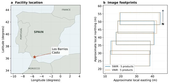
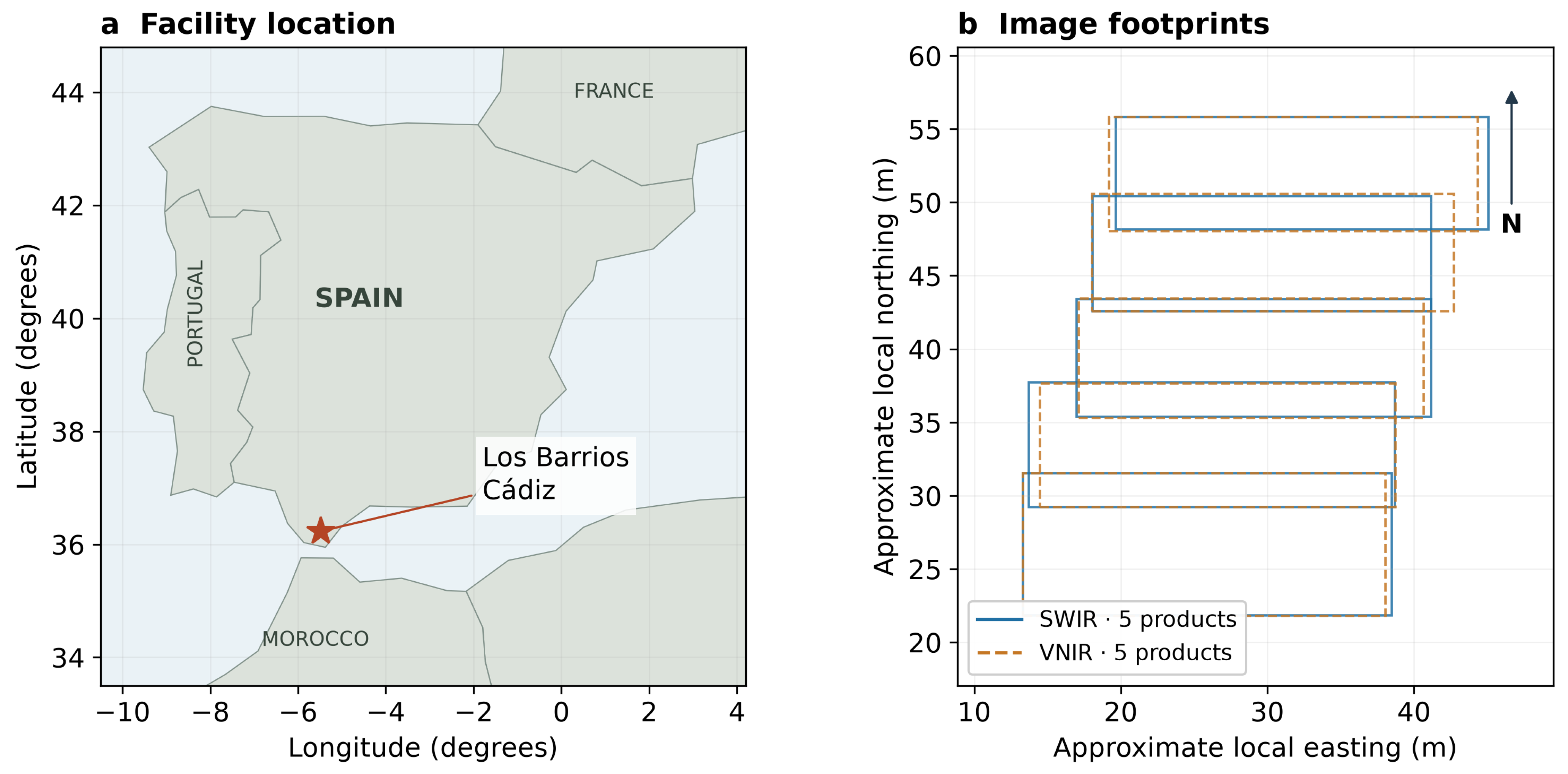
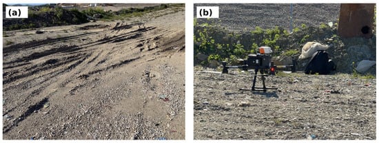
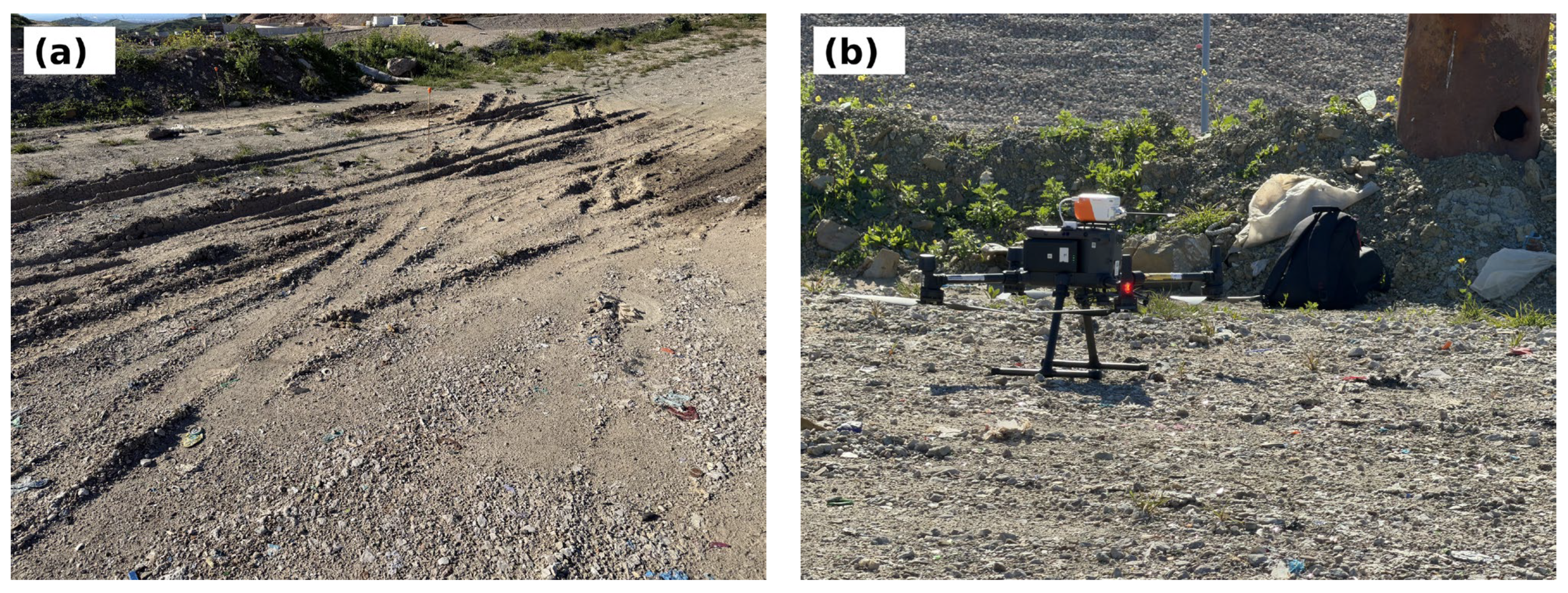
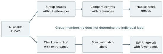
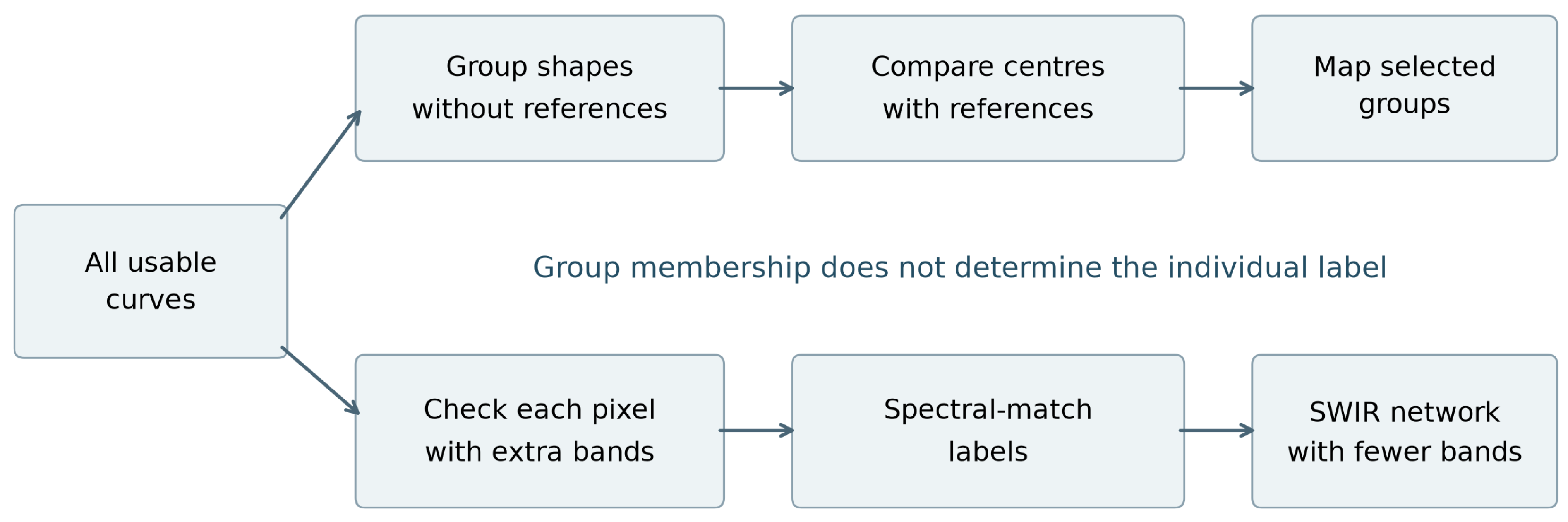
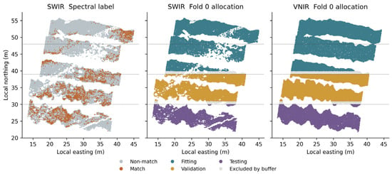
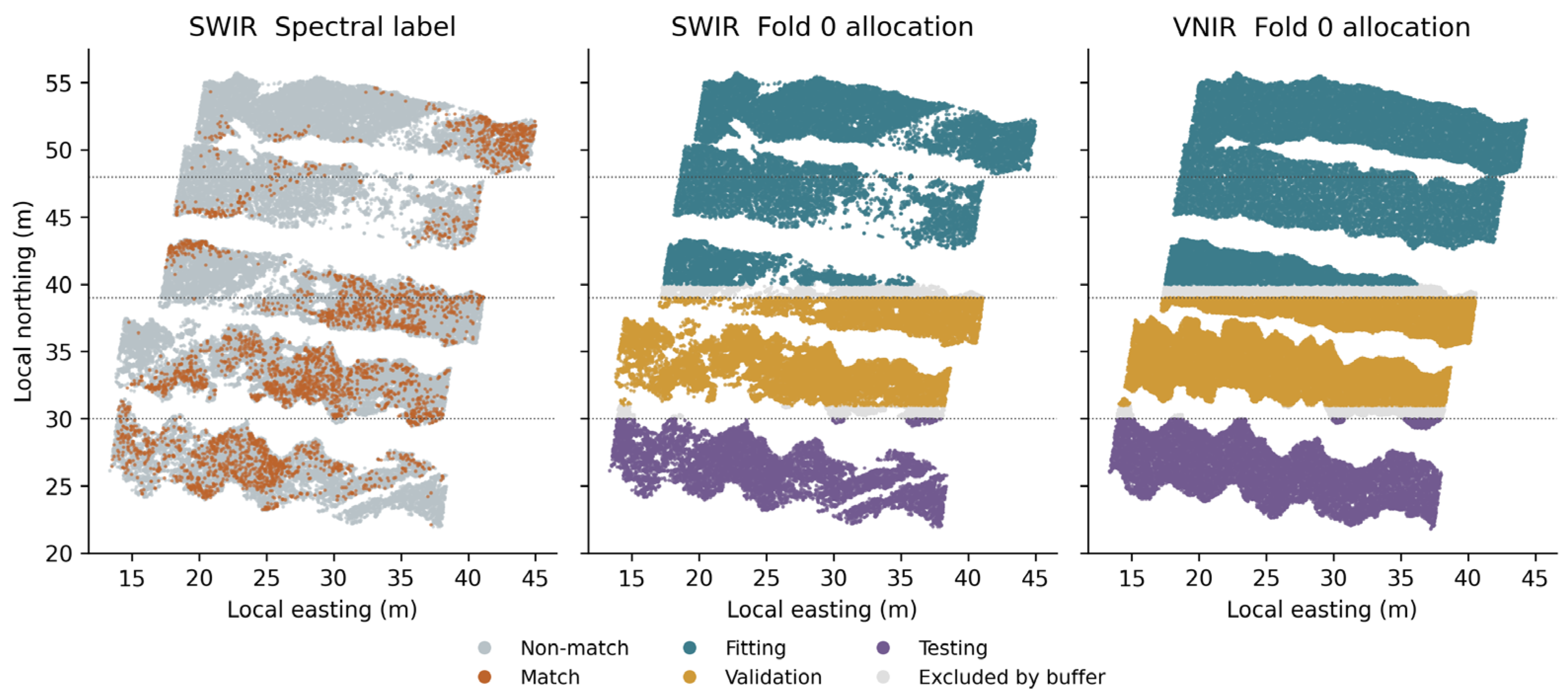
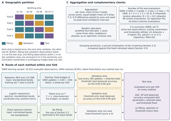
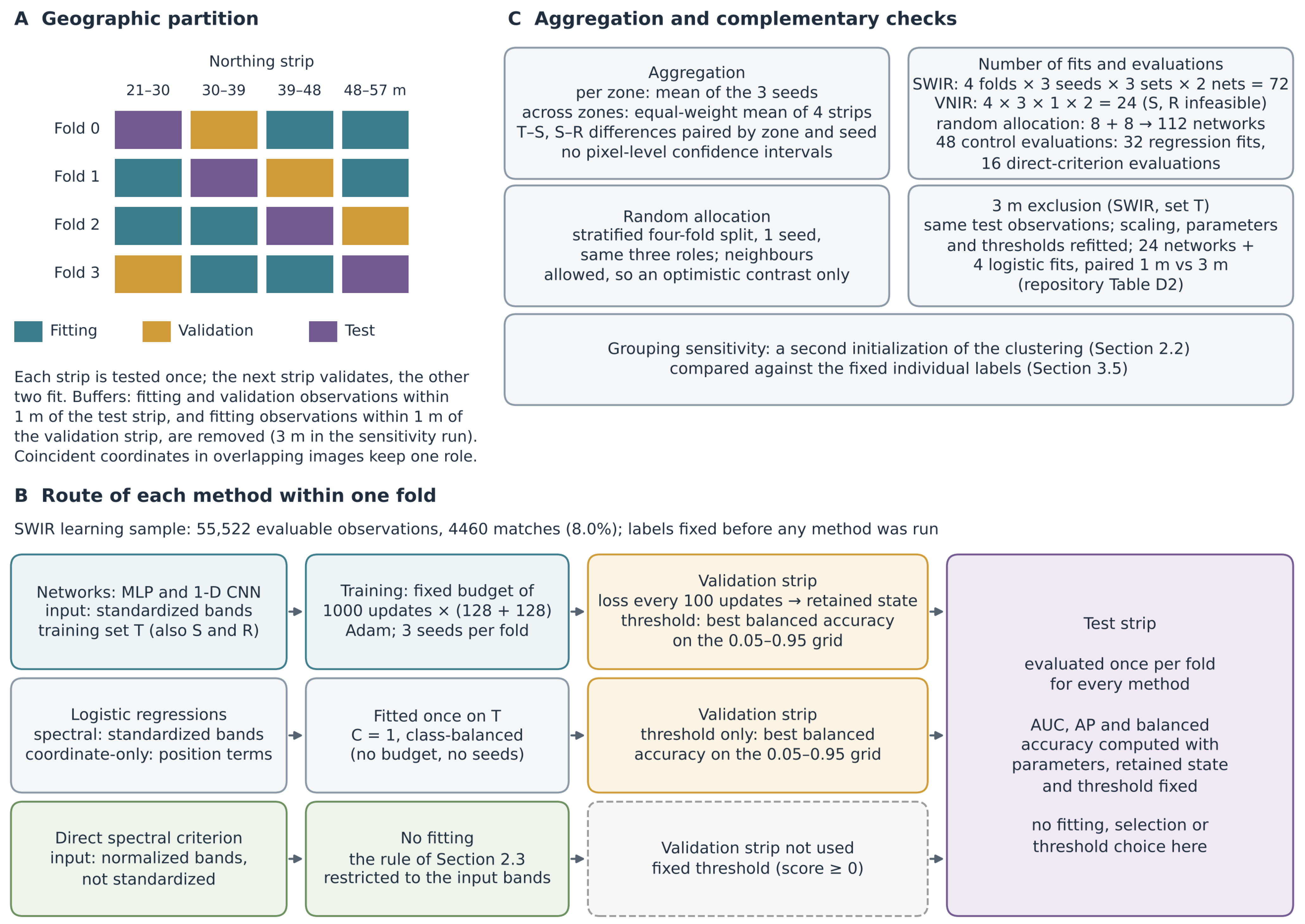
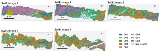
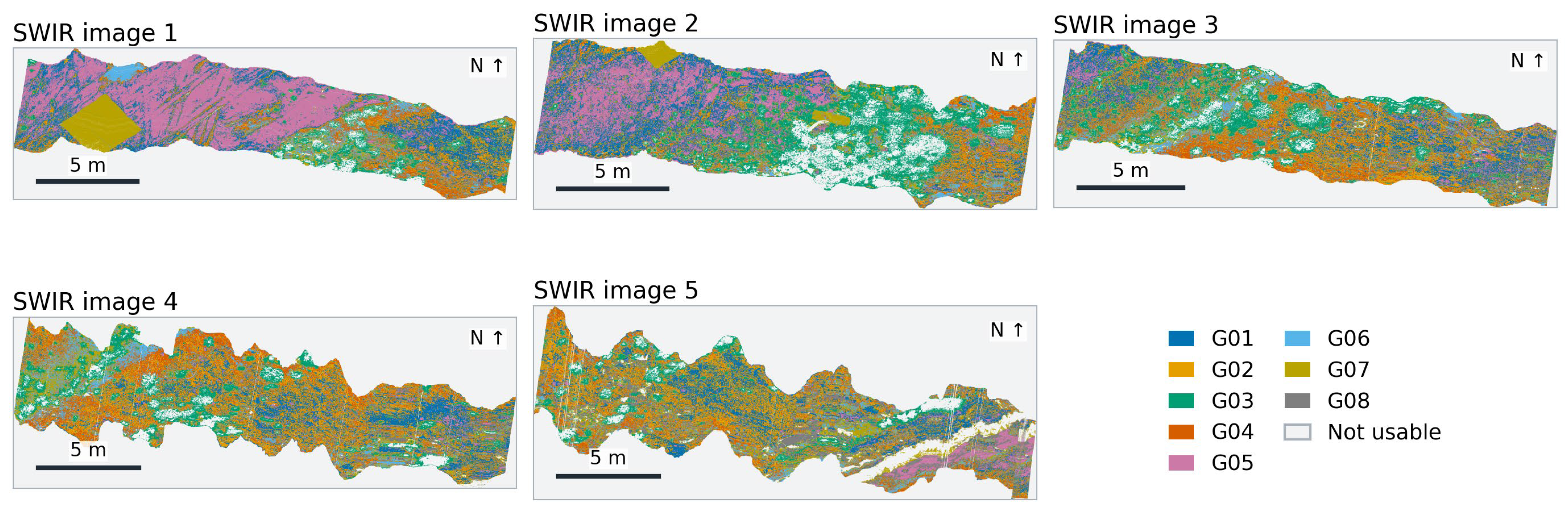
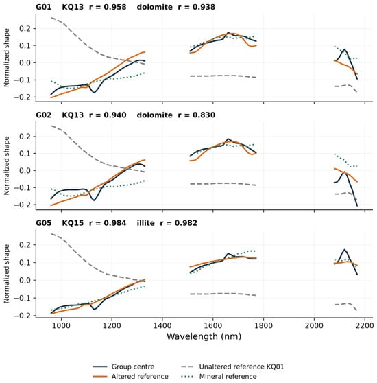
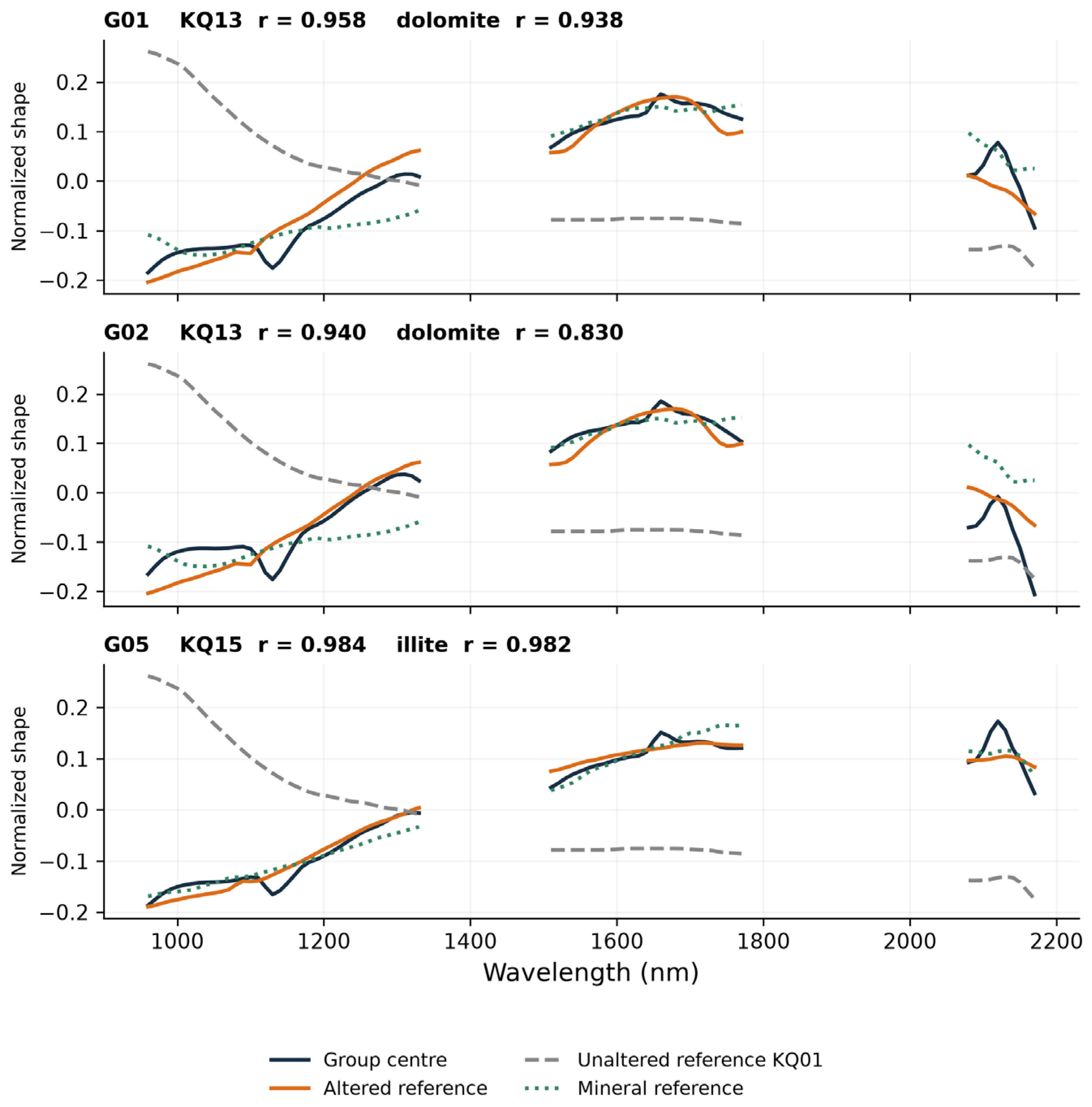
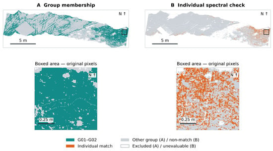
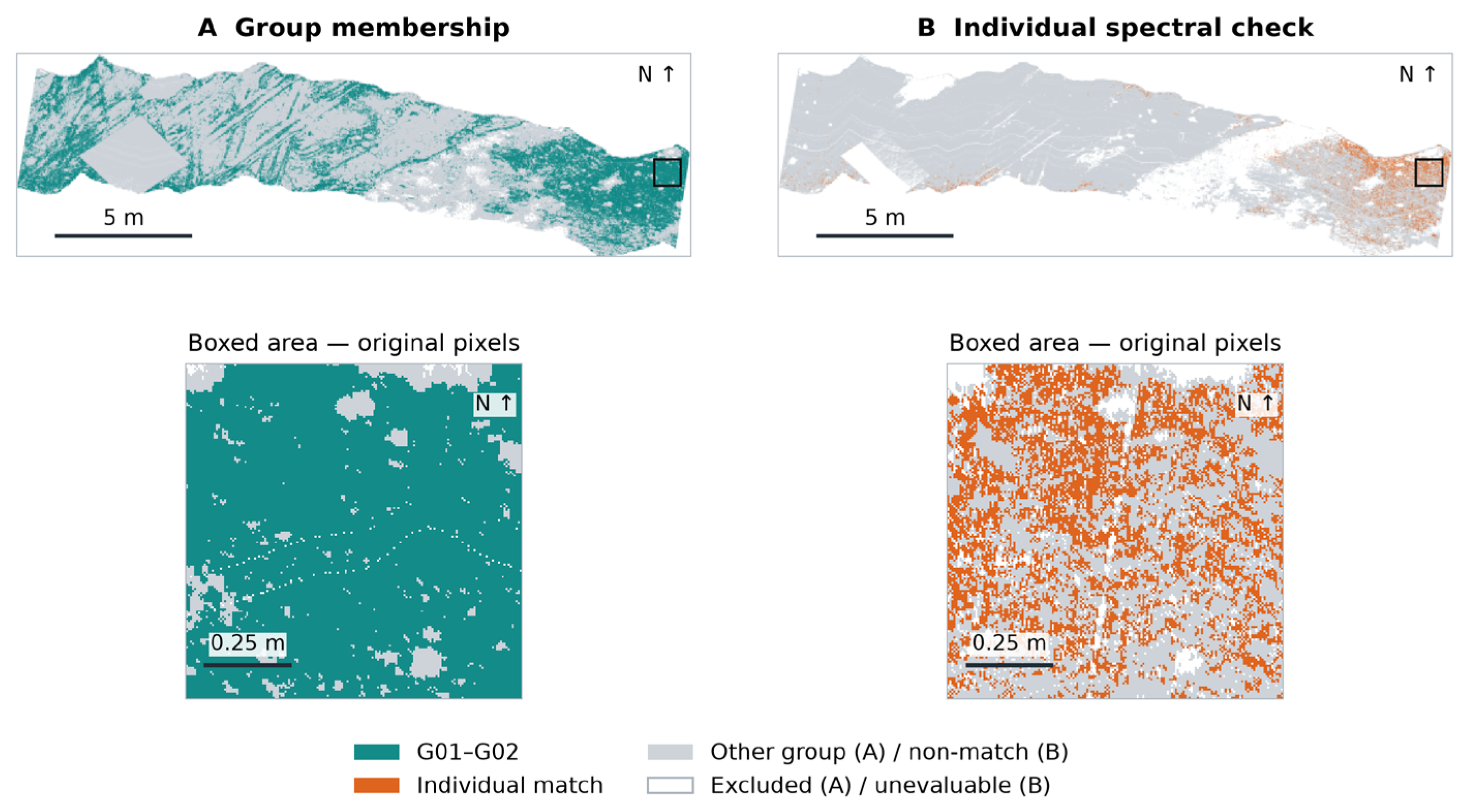
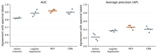
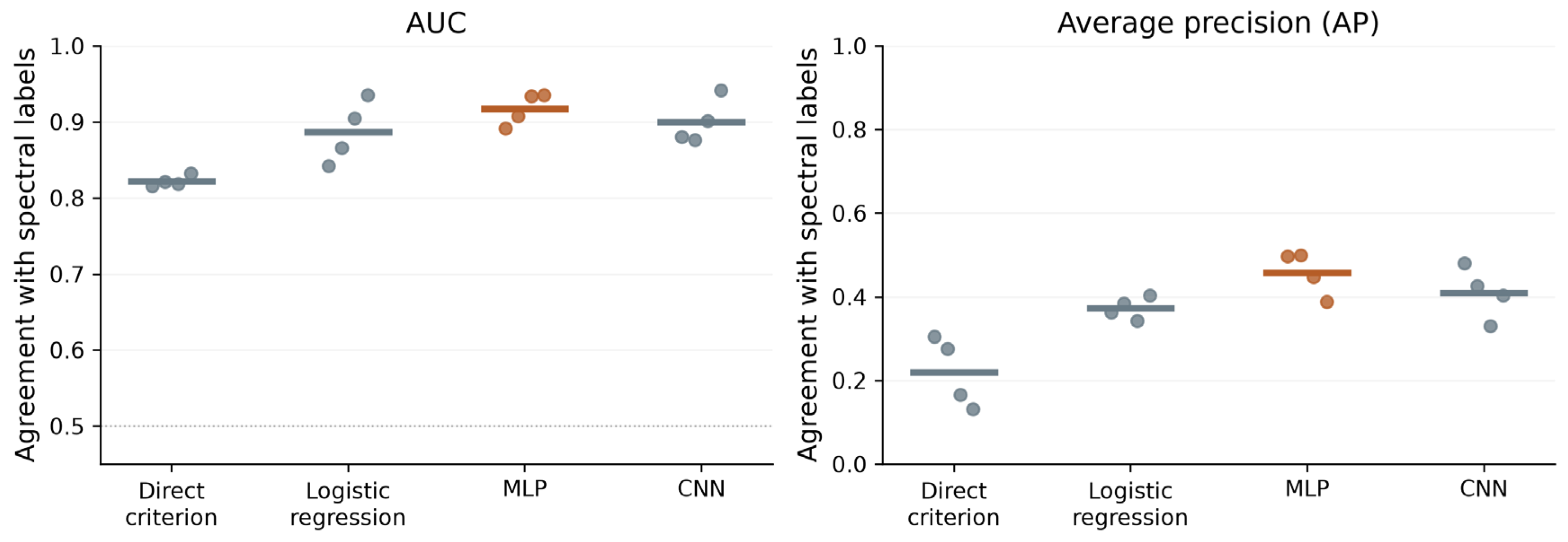

Disclaimer/Publisher’s Note: The statements, opinions and data contained in all publications are solely those of the individual author(s) and contributor(s) and not of MDPI and/or the editor(s). MDPI and/or the editor(s) disclaim responsibility for any injury to people or property resulting from any ideas, methods, instructions or products referred to in the content. |
© 2026 by the authors. Licensee MDPI, Basel, Switzerland. This article is an open access article distributed under the terms and conditions of the Creative Commons Attribution (CC BY) license.