Analysis of Radio Noise in a Mountain Radio Observation Station

Abstract

Radio noise at mountainous observatories affects the deployment of radio observation equipment. Existing mountainous-station measurements have mainly focused on spectrum occupancy and interference amplitude, while the statistical properties of the noise remain insufficiently addressed. To fill this gap, this study analyzes both the Gaussian and impulsive components of the noise. Radio noise in the 30–500 MHz band was measured at a high-altitude mountainous station in southwestern China using a USRP X310 software-defined radio. For the Gaussian component, the measured noise figure exceeds the ITU-R P.372-17 model and decreases with frequency. A smoothing spline model achieved an RMSE of 0.8687, an MAE of 0.3843, and an R² of 0.9929, outperforming the ITU-R P.372-17 model. For the impulsive component, pulse events were concentrated in the 30–140 MHz and 200–270 MHz bands. An XGBoost regression model was trained to predict IN level density and pulse length from statistical features and was benchmarked against linear, polynomial, and random forest baselines under leave-one-time-block-out cross-validation. These results provide empirical data and references for radio service deployment at mountainous observation stations.

1. Introduction

The radio noise at mountainous radio observatories presents unique challenges for the design and deployment of radio observation equipment. The radio noise in such scenarios primarily originates from a limited number of local devices within the site, such as transmission lines, lighting equipment, and vehicle engines. Moreover, impulsive components are frequently present in radio noise in addition to the Gaussian component. These impulsive components can severely degrade system performance, even under relatively high signal-to-noise ratio conditions. Consequently, a comprehensive statistical analysis encompassing both the Gaussian and impulsive dimensions is essential.

The analysis of radio noise relies on site-specific measurement data, thereby necessitating standardized measurement procedures [1,2]. Extensive studies have been conducted in various real-world environments, including office areas, industrial zones, vehicle traffic areas, urban areas, and residential districts [3,4,5,6,7]. Additionally, research has demonstrated a significant correlation between human-made noise and population density [8,9]. Existing studies on radio noise at mountainous stations have primarily focused on spectrum occupancy, occurrence frequency, and amplitude, rather than the statistical distribution of the noise itself. For instance, Sitompul et al. measured RFI from 70 MHz to 7 GHz at Mount Timau, Indonesia (altitude 1532 m), and used peak detection to characterize the occupancy of each sub-band [10]. In a similar vein, Küçük et al. in Turkey and Abidin et al. in Malaysia conducted RFI surveys for candidate radio astronomy sites [11,12]. A common feature of these studies is that they take spectrum occupancy as the core metric and interference source identification as the primary objective, with the analysis centered on the occurrence frequency and amplitude of interference signals rather than the statistical distribution of the noise itself.

The statistical characteristics of impulsive components and their impact on receivers have received considerable attention. Current mainstream approaches include the Gaussian mixture model [13], the Bernoulli–Gaussian model [14], the Middleton model [15], and the SαS stable distribution model [16,17]. For specific applications, ref. [18] proposed a two-state model based on damped sinusoidal waves for power-line communications, while [19] supplemented the measurement data for indoor elevator scenarios. To enhance model applicability, ref. [20] developed a novel simulation method for the Middleton Class A model, with a particular focus on its impact on BFSK and OFDM systems. Furthermore, ref. [21] introduced Markov chains to overcome the limitation of the Middleton Class A model, which only simulates amplitude distributions, thereby endowing the model with time-dependent characteristics.

Meanwhile, numerous studies have shown that the statistical characteristics of impulse components often exhibit different distribution patterns in various environments. Broadband measurements at 762 MHz conducted on Castellana Avenue and the Ascaso business district revealed that while impulse durations roughly followed a gamma distribution, other parameters did not conform to standard distributions [22]. In contrast, in factory environments, the power distribution of impulse components in the frequency domain can be described by a linear function of Gaussian distribution; whereas in the time domain, parameters such as amplitude, duration, and interval can be respectively fitted with Cauchy, gamma, and exponential distributions [23]. The statistical properties of impulse noise show significant differences in mathematical distributions across different regions, increasing the difficulty of analyzing impulse noise patterns. In comparison, current data-driven machine learning methods offer an alternative approach. Extreme Gradient Boosting (XGBoost) [24] is a supervised learning algorithm based on decision trees and gradient boosting techniques, which has demonstrated excellent performance in various radio applications, including radar signal classification [25], RF amplifier power modeling [26], wireless communication distance estimation [27], wireless environment modeling [28], and wireless link prediction [29].

Since radio noise significantly affects radio observation systems, this article aims to conduct an in-depth statistical analysis of the radio noise at a mountainous observatory, with a focus on its Gaussian background component and non-Gaussian impulsive component. Unlike the mountainous-station RFI studies in [10,11,12], which focus on spectrum occupancy and interference identification, this work analyzes the statistical properties of radio noise. The main contributions of this work are threefold. First, a dedicated measurement dataset of radio noise in the 30–500 MHz band has been established at a high-altitude (2054 m) mountainous radio observation station in southwestern China, providing empirical radio-noise statistics for a geographic region where such measurements have not been previously reported in the open literature. Second, for the Gaussian component, a smoothing spline regression model is adopted to capture the nonlinear frequency dependence of the noise figure in the 150–300 MHz range, where the conventional log-linear model recommended by ITU-R P.372-17 fails to describe the observed variations. Third, for the impulsive component, IN level density and pulse length are predicted using an XGBoost regression model trained on statistical features, with performance benchmarked against linear, polynomial, and random forest baselines under leave-one-time-block-out cross-validation.

2. Measuring Method

2.1. Measurement Equipment

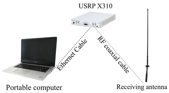
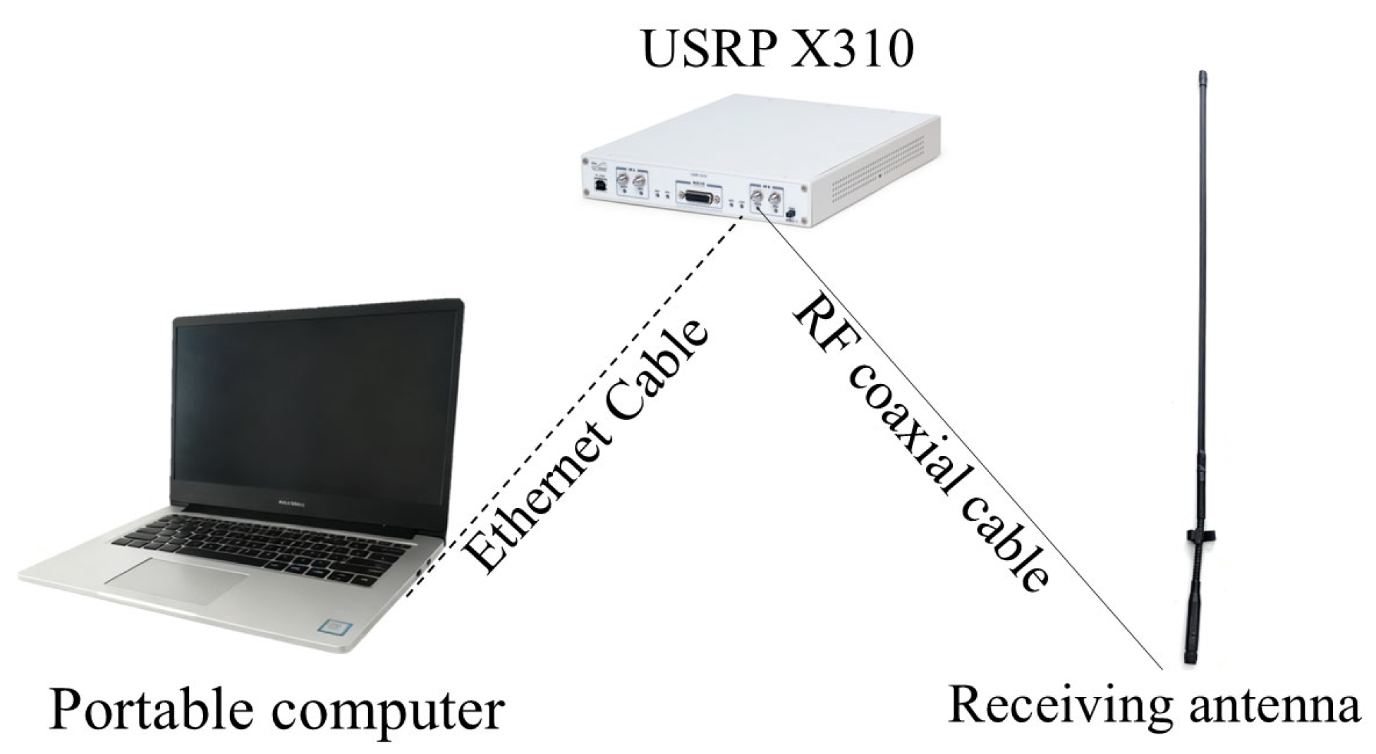
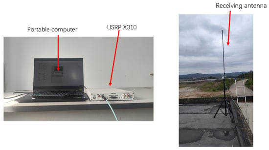
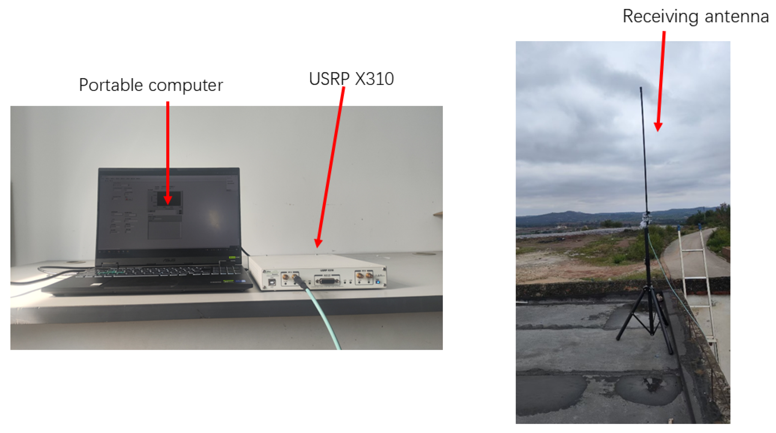
The measurement equipment employed in this study comprises the USRP X310 (manufactured by Ettus Research, Austin, TX, USA), a receiving antenna (manufactured by Wuhan Zhongdian Communication Co., Ltd., Wuhan, China), and a portable computer. A schematic diagram of the equipment is presented in Figure 1. The USRP X310 is a software-defined radio platform that enables the sampling of wireless signals in the form of IQ data. The receiving antenna is a vertical monopole antenna operating from 30 MHz to 676 MHz, with an input impedance of 50 Ω, a length of 1.3 m, and a gain of −4 dB. A portable computer controls the USRP X310 to sample anthropogenic radio noise by configuring parameters such as sampling frequency, bandwidth, sampling rate, and gain using LabVIEW 2020 and the USRP Hardware Driver (UHD) 4.0. The specific parameter values are shown in Table 1. The gain values for different frequencies of the preamplifier are listed in Table 2.

Figure 1. Schematic diagram of the measurement equipment.

Table 1. Measured parameters.

Parameter	Value
Frequency range	30–500 MHz
Frequency interval	1 MHz
Preamplifier gain	dynamic gain
Measuring bandwidth	2 MHz
Sampling rate	2 MHz
Time resolution	500 ns
Duration of each sampling	2 s
Antenna height	5 m

Table 2. The gain of the preamplifier.

Frequency (MHz)	Gain (dB)
30–34	10
34–48	15
49–64	20
65–149	23
150–166	25
167–188	27
189–228	30
228–500	35

2.2. Measurement Area

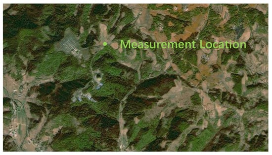
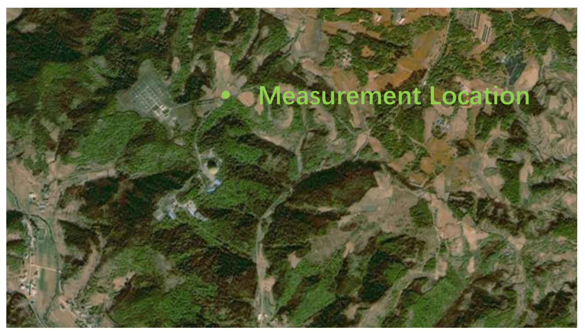
The mountainous observation station in Qujing was selected as the measurement site for the mountainous area survey in this study. The coordinates are 25.641285° N latitude and 103.715625° E longitude, with an elevation of 2054.38 m. The measurement area is illustrated in Figure 2.

Figure 2. Measurement location.

The mountainous radio observation station is situated outside major residential areas and main traffic routes, implying that external interference signals are virtually absent. The primary sources of internal radio noise include transmission lines, lighting equipment, office electronic devices, and a limited number of vehicle engines. In addition, radio observation equipment deployed at the site emits radio signals that interfere with the measurement and analysis of radio noise.

2.3. Measurement Process

The entire data measurement process involves the USRP X310 device capturing environmental radio noise via the receiving antenna, subsequently transmitting the signal to a portable computer through the transmission line for local storage, followed by processing and analysis. Continuous periodic measurements were conducted across the frequency range of 30 to 500 MHz over a total duration of 24 h. The receiving antenna was positioned at a height of 5 m above ground, as illustrated in Figure 3.

Figure 3. Measurement equipment placement.

3. Interference Signal Processing

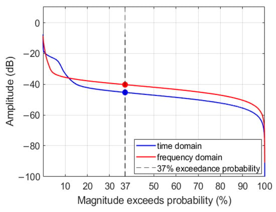
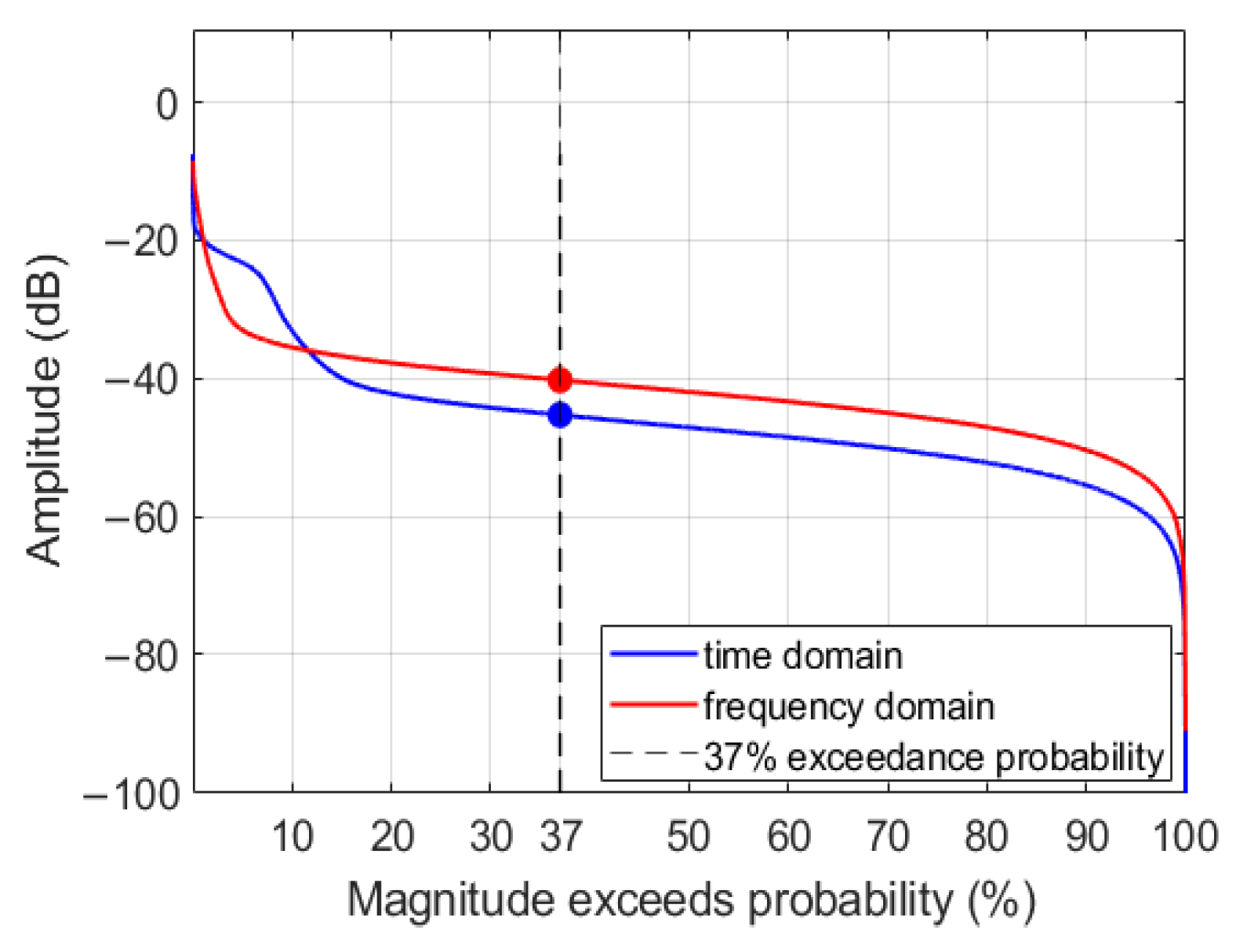
It is challenging during actual measurements to ensure that the measured frequency band remains free from interference by radio services, which adversely affects radio noise analysis. ITU-R SM.1753-2 provides a method for interference signal exclusion, which compares frequency bands and retains portions unaffected by interference. The first step of the interference signal exclusion method involves excluding data samples whose median value exceeds a specific threshold. The sampled data are grouped, with each group consisting of 50 samples. Groups whose median exceeds the overall root mean square (RMS) value of the sampled data are excluded, along with the two adjacent groups immediately before and after. The RMS value is determined based on the amplitude probability distribution (APD). When narrowband interference signals or single-carrier noise are present, the Fourier transform is applied to convert the time-domain signal to the frequency domain, and the final RMS value is taken as the lower of the two values corresponding to the 37th percentile from the APDs in the time and frequency domains.

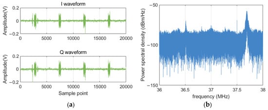
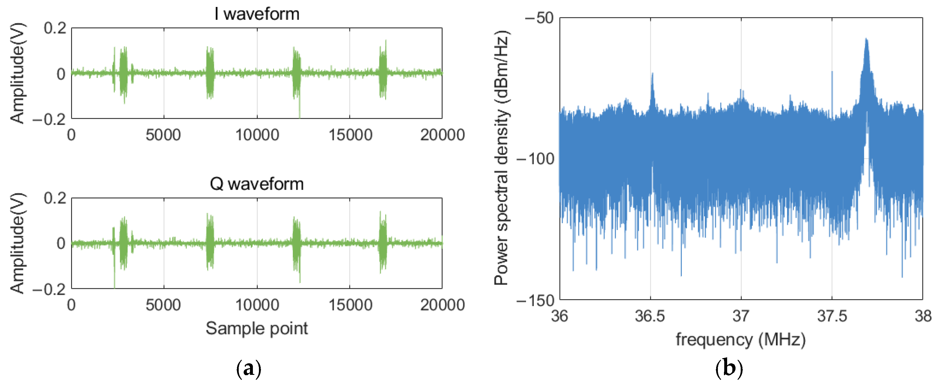
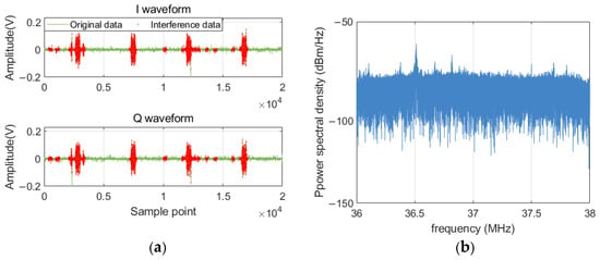
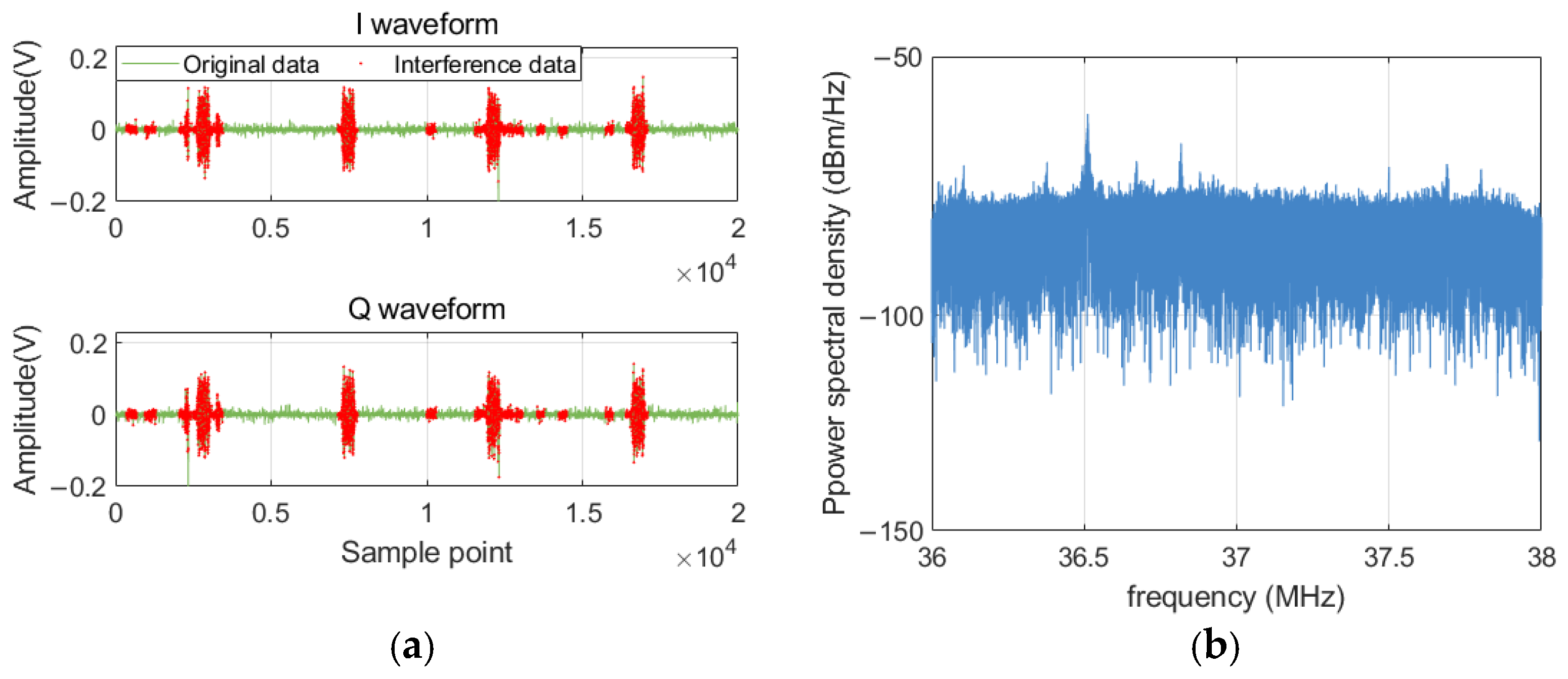
Figure 4 shows a set of raw data collected at the 37 MHz frequency point, including an interfering signal. The center frequency of this interference is 37.7 MHz, with a bandwidth of 100 kHz and a peak level of −41.77 dBm/Hz.

Figure 4. Data at the 37 MHz frequency point with interference signals: (a) IQ waveform, (b) power spectral density.

Figure 5 shows the amplitude probability distribution of the data magnitude and power spectral density. When the exceedance probability is 37%, the time-domain amplitude is −45.7531 dB, and the power spectral density amplitude is −40.126 dB. The smaller of the two values is taken as the threshold to exclude data points whose time-domain amplitudes exceed this threshold. The exclusion results are shown in Figure 6. High-amplitude interference signals are identified and removed; after exclusion, the value at 37.7 MHz in the power spectral density is −64.9 dBm/Hz, a reduction of 23.13 dB. It can be seen that while interference signals are being removed, some quiet samples are also excluded; however, this is acceptable in order to ensure the absence of interference signals.

Figure 5. The amplitude probability distribution of amplitude and power spectral density.

Figure 6. 37 MHz measurement data exclusion results: (a) IQ waveform, (b) power spectral density.

The second step involves excluding frequency points that contain intentional radio signals. Radio noise is measured at two or more frequencies within the target frequency band. Subsequently, the RMS is determined for each measurement frequency, and all data samples with RMS values exceeding the minimum RMS value are excluded.

In the actual processing, to mitigate the intermittent effects of radio service interference signals, frequencies within each measurement cycle are grouped at 5 MHz intervals, with multiple periodic comparisons performed. Additionally, the relationship between the voltage RMS value and power, as expressed in (1), is considered, enabling the voltage RMS magnitude to be mapped to the power level.

$$P_m={\displaystyle \frac{V_{\mathit{rms}}^2}{R}}$$

(1)

where P_m represents the power of the collected data, $V_{\mathit{rms}}^2$ denotes the root mean square value of the voltage, and R is the load impedance of the antenna.

Considering the application of different preamplifier gains for various frequency bands during the measurement process, along with the inherent system noise of the measurement system, the data power is calculated to accurately reflect the true magnitude relationships of the external environmental radio noise. The data power after excluding irrelevant interferences is calculated, as shown in (2). Subsequently, within each measurement period, the data are grouped at 5 MHz frequency intervals, and frequencies within each group whose power value exceeds the minimum power value by more than 2 dB are excluded. The 2 dB threshold follows the recommended value in ITU-R SM.1753-2 [1], which specifies that r.m.s. levels exceeding the lowest value by more than about 2 dB should be discarded in order to exclude frequencies affected by wanted emissions while retaining the local noise floor.

P_n = P_m − P_s − G_L

(2)

where G_L denotes the preamplifier gain, and P_s indicates the internal noise power of the measurement system. The method for obtaining P_c involves substituting the receiving antenna with a 50 Ω load impedance to connect to the IQ sampling channel, followed by acquiring IQ signals using the USRP X310, with acquisition parameters consistent with those presented in Table 1 and Table 2. The power computed from the acquired samples corresponds to the internal noise power of the measurement system.

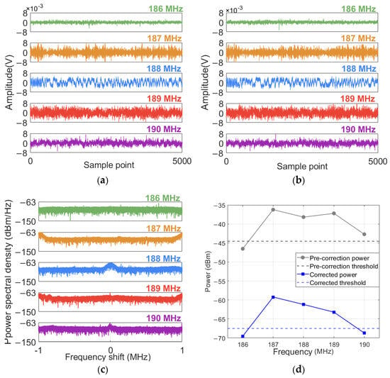
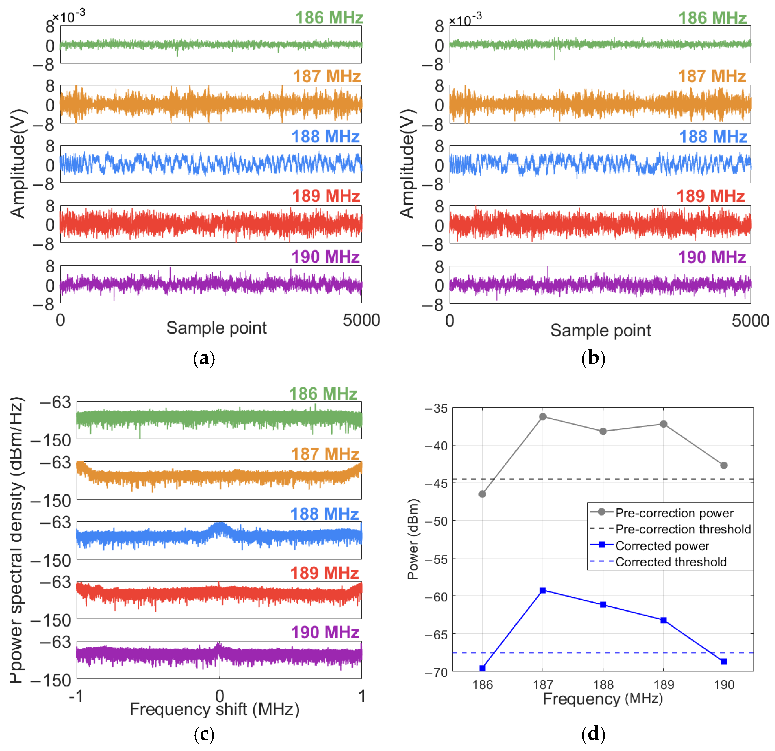
Figure 7 presents a set of data collected within the 186–190 MHz frequency band and the comparison of two experimental methods. In this set of data, the preamplifier gain in the 186–188 MHz frequency band is 27 dB, and the preamplifier gain in the 189–190 MHz frequency band is 30 dB. There is an interference signal with a center frequency of 188 MHz, a peak of −65.76 dBm/Hz, and a bandwidth of 200 kHz. Due to the sampling bandwidth of 2 MHz, the actual influence range of the interference signal extends to the data measured at the frequencies of 187 MHz and 189 MHz.

Figure 7. The collected data within the 186–190 MHz range with interference signals: (a) I waveform, (b) Q waveform, (c) power spectral density, (d) comparison before and after correction.

Figure 7d shows that when data is processed using the ITU-R SM.1753 method, due to the combined influence of the gain difference between the preamplifier and the internal noise of the receiver, the measured power at the 190 MHz frequency point is higher than the set threshold. This deviation results in this frequency point being wrongly identified as being affected by an interference signal and being excluded. By using the improved interference signal exclusion method for processing, the power at the 190 MHz frequency point drops below the threshold, avoiding the incorrect exclusion.

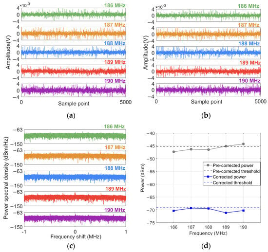
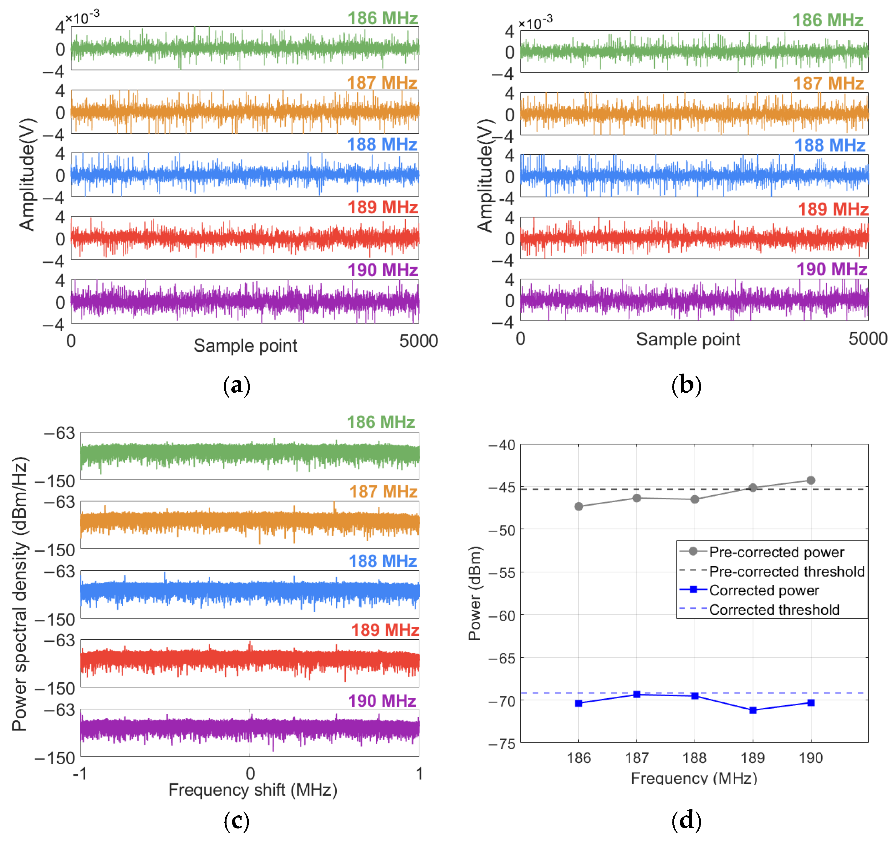
Figure 8 presents a set of data collected within the 186–190 MHz frequency band without interference signals, as well as the experimental comparison of the two methods under this condition. Figure 8d indicates that due to the influence of the preamplifier gain and internal noise, the power of the measurement data at the 189 MHz and 190 MHz frequencies is higher than the threshold. By correcting the power using the improved interference signal exclusion algorithm, the power at the 189 MHz and 190 MHz frequencies drops below the threshold.

Figure 8. Collected data within the 186-190 MHz range without interference signals: (a) I waveform, (b) Q waveform, (c) power spectral density, (d) comparison before and after correction.

The above results indicate that the method can effectively eliminate the influence of interference signals, as well as differences in preamplifier gain and internal receiver noise on power measurements.

4. Analysis of White Gaussian Noise

The level of radio noise is usually expressed by the noise figure. According to ITU-R SM.1753-2, when the frequency is higher than 60 MHz, the radiation efficiency of the antenna is usually high, and the antenna loss is almost negligible, which can be approximately regarded as a lossless antenna. In this case, the noise figure is calculated using (3).

F_a = P_n − P₀ − G_ant

(3)

where P_n is the sampling noise power and P₀ is the thermal noise power, as shown in (4). G_ant is the gain of the receiving antenna.

P₀ = 10log(K ⋅ t ⋅ b)

(4)

where K is the Boltzmann constant, and K = 1.38 × 10⁻²³ (J/K), t is the ambient temperature (K), taken as 297 K, b is the measurement bandwidth (Hz).

When the frequency is below 60 MHz, due to the relatively small physical size of the antenna relative to the wavelength, the radiation efficiency decreases and the loss increases. The assumption that the antenna is lossless no longer holds true. In this case, the average antenna coefficient is used to calculate the external noise coefficient:

F_a = P_n + AF − 20log(f) − 10log(b) + 202.5

(5)

where f is frequency (MHz) and represents AF the antenna coefficient, as shown in (6).

AF = 20log₁₀(f) − G_ant − 29.78

(6)

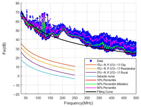
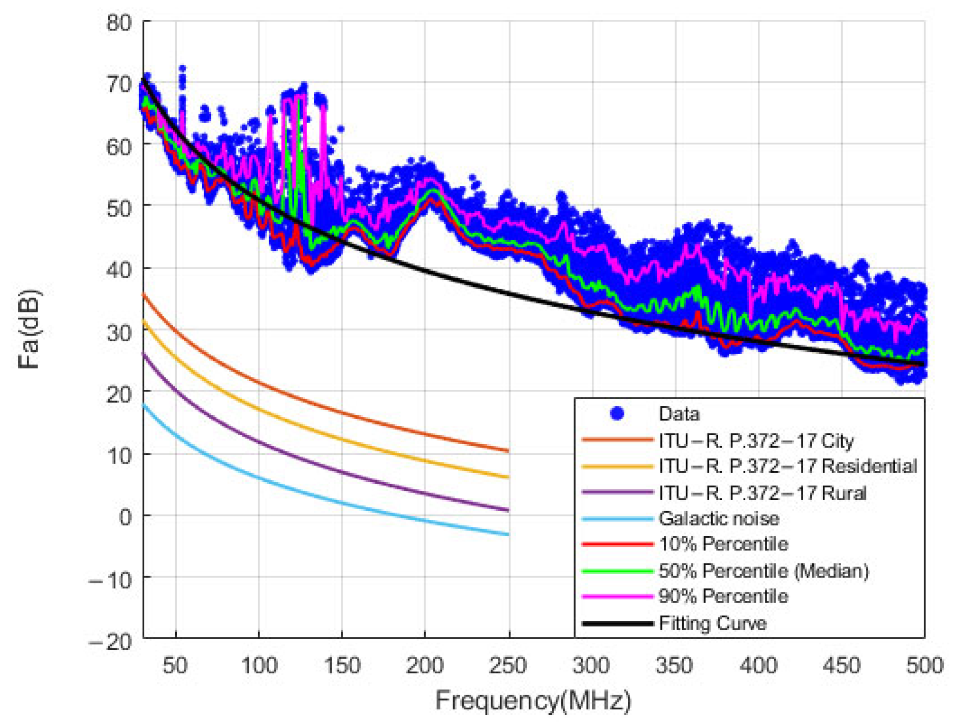
The calculated F_a values are depicted in Figure 9. For analytical comparison, the figure also incorporates the man-made noise models under various areas from ITU-R P.372-17, which delineate the variation trends of the median.

Figure 9. Noise figure value distribution.

Additionally, it includes the statistical quantiles of F_a values at different frequencies, specifically the 10th, 50th, and 90th percentiles. Furthermore, a new parametric model is presented, which adopts the same functional form as the ITU-R P.372-17 man-made noise model. The least squares estimation is employed to fit the median data values, thereby representing the overall trend in the data. The formula is given in (7).

F_am = a₀ + a₁ log f

(7)

The results derived from the figure indicate that the values of F_a substantially exceed the reference values provided in ITU-R P.372-17 while exhibiting a gradual decrease with increasing frequency.

Furthermore, the fitted model employing the same functional form as that in ITU-R P.372-17 generally underestimates the median values within the 150–300 MHz range and fails to accurately capture the actual variations in these median values. This implies that the actual data no longer strictly adhere to a linear relationship with the logarithm of frequency.

To capture these nonlinear characteristics, smoothing spline regression was employed to fit the data. It does not assume a linear or specific polynomial form for the data relationship. Instead, it fits the curve using piecewise polynomials while ensuring smooth transitions at the knots. This approach enhances its flexibility in capturing local variations. A spline function is a piecewise polynomial function, represented by polynomials within each interval, while maintaining continuity at the boundaries between intervals. In general, the spline function is defined through a piecewise polynomial. For smooth spline regression, the spline can be defined as follows:

S(x) = S_j(x) → x ∈ [x_j,x_j+1],    j = 1,…,n − 1

(8)

where S_j(x) represents the spline basis function, which is a cubic spline function, with its formula provided in (9).

S_j(x) = a_j + b_jx + c_jx² + d_jx³

(9)

The objective of smoothing spline regression is to identify a smooth curve that minimizes the data fitting error while ensuring the curve’s overall smoothness. The objective function for smoothing spline regression is defined as follows:

$$\min {\displaystyle {\displaystyle \sum _{i=1}^n}(y_i-S(}{x}_i){)}^2+\mathit{\lambda }{\displaystyle {\int }_{-\infty }^{\infty }(S^{″}(}x){)}^2\mathit{dx}$$

(10)

The first item is to minimize the fitting error. The second term is the smoothing term, which controls the smoothness of the spline function. S^″(x) represents the second derivative of S(x), measuring the curvature of the curve. λ is the regularization parameter, which governs the trade-off between the smoothness term and the fitting term.

It is important to note that the performance of the smoothing spline depends on the choice of the parameter λ. When λ is large, the spline function becomes smoother; when λ is small, the fitting error dominates, potentially leading to overfitting. By traversing the values of λ, the optimal value of λ can be determined, which minimizes the mean squared error.

To ensure numerical stability, five-fold cross-validation is used to select the optimal λ parameter, ensuring robustness. The cross-validation error (CV error) is used as an alternative to the mean squared error. The process is as follows: after setting a specific value of λ, the data are randomly divided into five groups. One group is used as the validation set, and the remaining four groups serve as the training set. The spline regression model is applied to the training set, and the CV error is calculated using the validation set. After calculating the CV error for each fold, the average of the five-fold CV errors is taken as the final CV error.

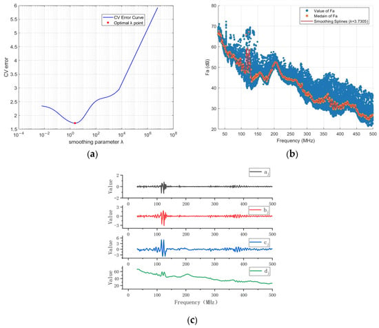
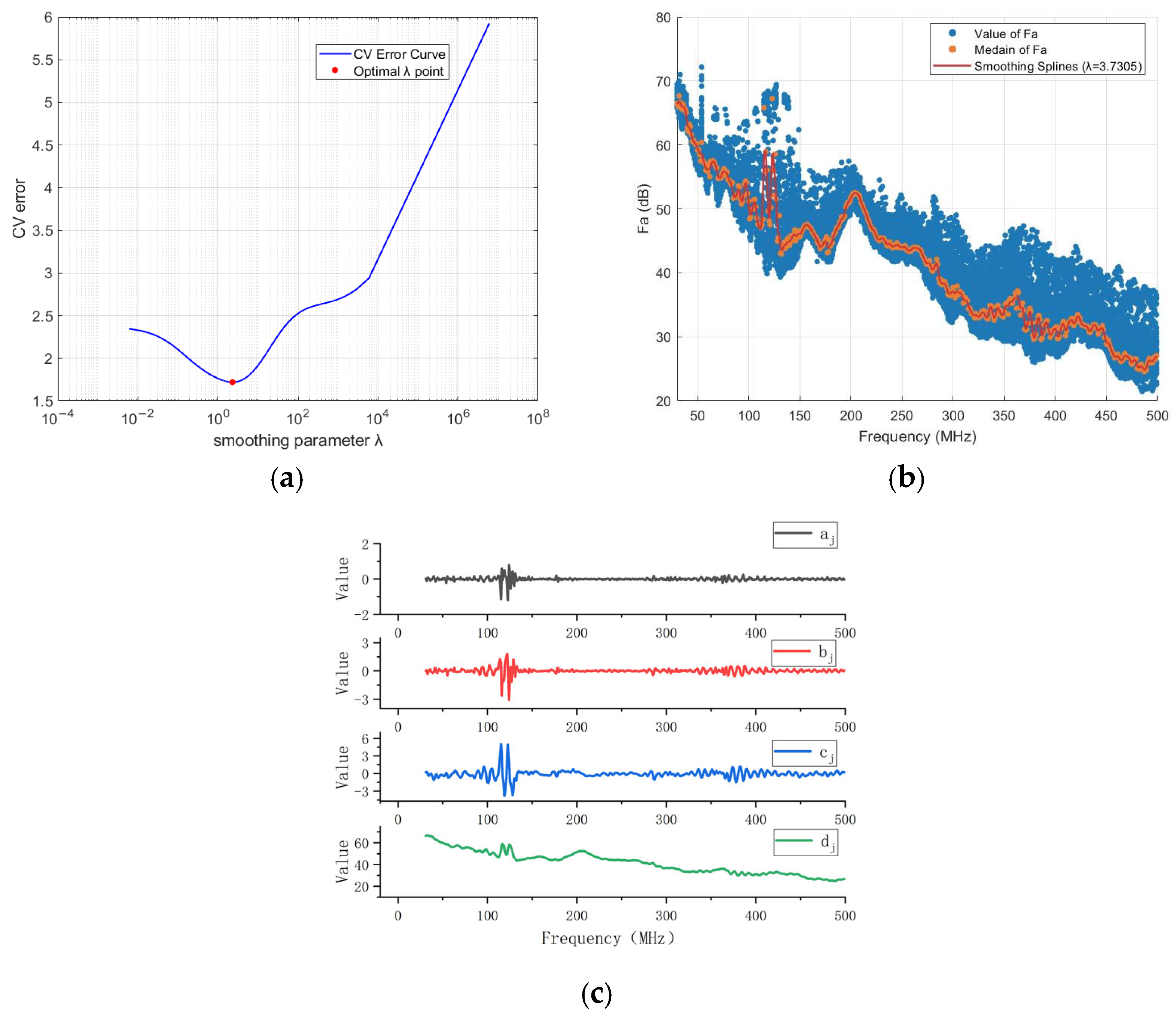
The relationship between the CV error and different values of λ is illustrated in Figure 10a. The figure highlights the value of λ that minimizes the CV error, which serves as the optimal λ. Figure 10b presents the smoothing spline regression curve obtained under this optimal λ value, while Figure 10c displays the coefficient values for each cubic polynomial in the smoothing spline regression model. The smoothing spline curve corresponding to the optimal λ is compared with both the newly fitted log-linear model and the ITU-R P.372-17 model for the urban area, which best approximates the measured values. Subsequently, performance metrics including RMSE, MAE, and the coefficient of determination R² are calculated, as summarized in Table 3.

Figure 10. Smoothing spline regression for the noise figure. (a) Relationship between the CV error and different values of the regularization parameter λ. (b) Distribution of the noise figure F_a with the optimal λ = 3.7305. (c) Coefficient values for each cubic polynomial in the smoothing spline regression model with λ = 3.7305.

Table 3. Performance comparison of ITU-R P.372-17 model, Log-linear model, and Smoothing Splines model.

Parameters	ITU-R P.372-17 Model	Log-Linear Model	Smoothing Splines Model
RMSE	29.8513	5.3433	0.868780
MAE	29.5954	4.2490	0.384351
R2	−7.3187	0.7335	0.992954
AIC	4530.25	1065.42	883.85

It is evident that the Smoothing Spline model improves the goodness of fit compared to the other models. Specifically, it yields superior RMSE, MAE, and R² values. Furthermore, the model achieves a lower AIC, indicating a better balance between fitting accuracy and model complexity.

However, this improvement in accuracy comes at the expense of increased complexity, as the model involves four frequency-dependent parameters. It is also important to note that this model is valid only for characterizing radio noise within the 30–500 MHz frequency range. Since the parameters are specific to the variations observed in this band, the model is unsuitable for extrapolation to other frequencies. Therefore, caution should be exercised when applying this model.

5. Analysis of Impulse Noise

In actual practice, radio noise, in addition to the WGN component, often contains impulse components. One prerequisite for analyzing pulse components is to extract them from radio noise. In addition, when examining the variation in the radio frequency amplitude of the actual pulse over time, most pulses are a series of short peaks or “pulse sequences”. Since the measurement of the pulse level of radio noise mainly focuses on the interference potential of the pulse, it is necessary to integrate the peaks of the pulse sequence into a single event known as a “burst”. ITU-R SM.1753-2 presents a method, and the steps are as follows.

5.1. Separation of Impulse Noise

• First, a threshold much higher than the WGN peak was set for extracting the IN component. This threshold is set at a level 13 dB higher than the RMS value of WGN. This 13 dB threshold follows the recommendation in ITU-R SM.1753-2 [1], which specifies that the threshold should be set 13 dB above the r.m.s. WGN level, since this value corresponds to the typical CREST factor (the difference between the r.m.s. and peak values) of WGN. All samples above this threshold are treated as IN.
• Merge the samples that are continuously above the threshold into a set and determine the center point C_p of this set.
• Start from C_p and count the number of samples N that exceed the threshold to the right.
• At the end of the sample, check whether there are any samples within the subsequent N samples that exceed the threshold. If new samples are found to exceed the threshold before N samples, these samples will be included in the original pulse, and we will obtain a new pulse set.
• Determine the center point C₁ within the new pulse set once again.
• Count the number of samples N₁ that exceed the threshold to the right of the center point C₁ of the new pulse set once again.
• At the right end of the new pulse set, check the samples that are above the threshold among the subsequent N₁ samples. If new samples above the threshold are found, they should be included again to form a new set of pulses. Then determine the center point C₂ of the new pulse set once again. Repeat steps 4 to 6 until no new samples are found.
• Perform steps 4 to 6 on the left end of the updated pulse set until no new samples are found on the left end. The final set of pulses is a pulse burst event.
• Repeat steps 2 to 7 for the next pulse set.

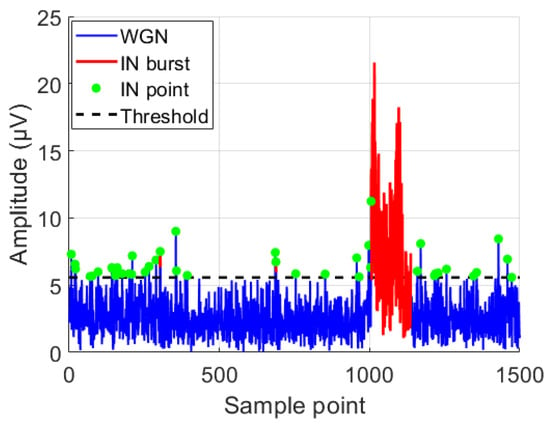
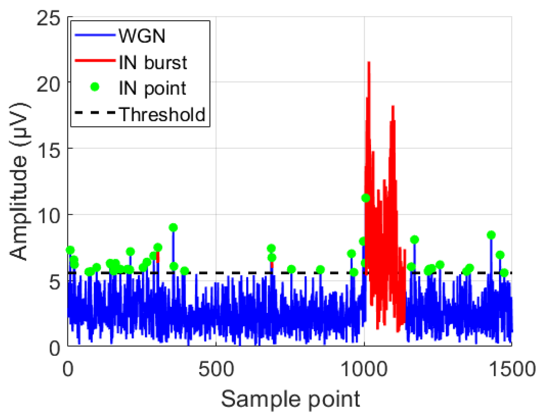
This process ensures that more than 50% of all samples within each pulse are above the threshold, and this condition is also continuously met during the “growth” of the pulse. Therefore, some peaks in the irregular pulse sequence are combined into a single, long burst. Figure 11 shows the IN burst identification process for a set of data sampled at 190 MHz. The blue curve represents the WGN component, the black dashed line indicates the IN threshold set according to ITU-R SM.1753-2, the green dots denote the samples exceeding the threshold, and the red curve represents the pulse bursts formed by merging these samples following the method described in ITU-R SM.1753-2 § 10.9.

Figure 11. Identification of impulsive noise bursts in sampled data at 190 MHz.

Following the extraction of the IN component, it is also essential to analyze the statistical distribution information of the pulse parameters. These parameters aid in characterizing the features of interference noise and facilitate further analysis and processing. The specific parameters include total impulse length, IN level density, and pulse length.

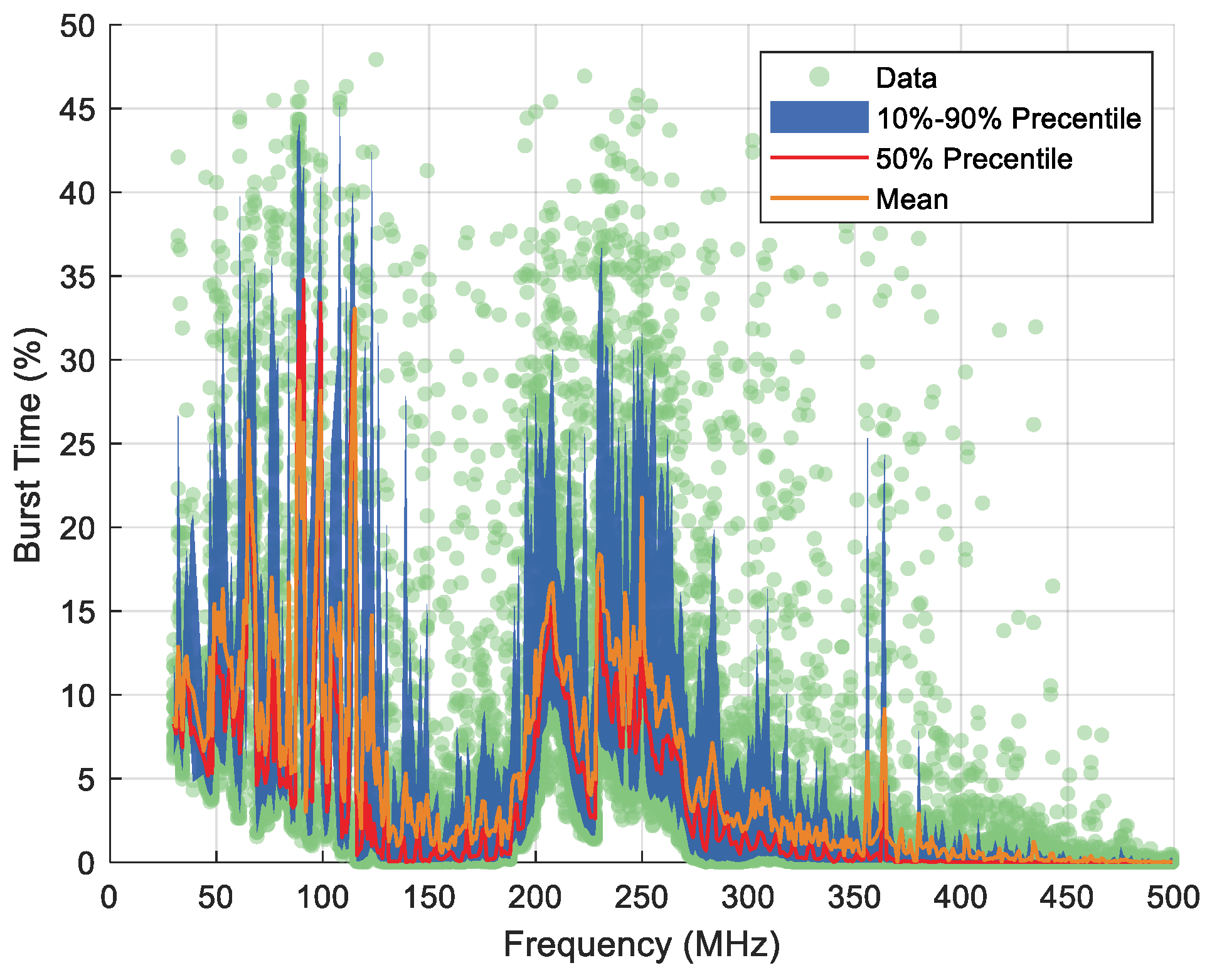
The total impulse or burst time is given as a percentage of the total survey time:

i = (N_i / N) × 100%

(11)

where N_i is the number of samples above the IN threshold. N is the total number of measurement samples.

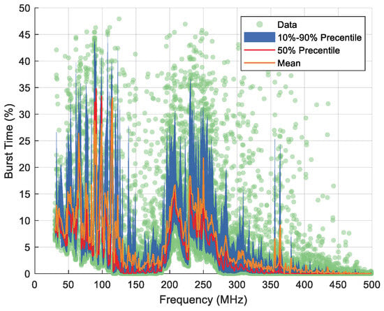
The statistical results of the total impulse or burst time of the measured samples are shown in Figure 12.

Figure 12. Statistical results of the total impulse or burst time as a percentage of the total survey time.

The impulse level denotes the signal strength of the measured pulse or burst. Given that this level is contingent upon the bandwidth of the measurement system, the measurement results are normalized to the bandwidth employed to achieve independence from the measurement bandwidth. Consequently, the IN level is expressed as a level density. The calculation formula is as follows.

W_g = U + 20log(1 / b)

(12)

where W_g is spectral density (dBμV/MHz). U is measured noise voltage from the receiving antenna (dBμV). b is noise bandwidth (MHz).

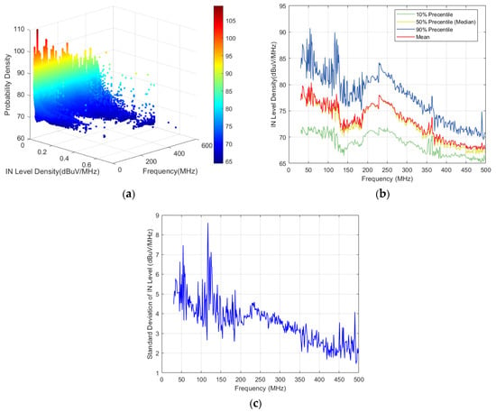
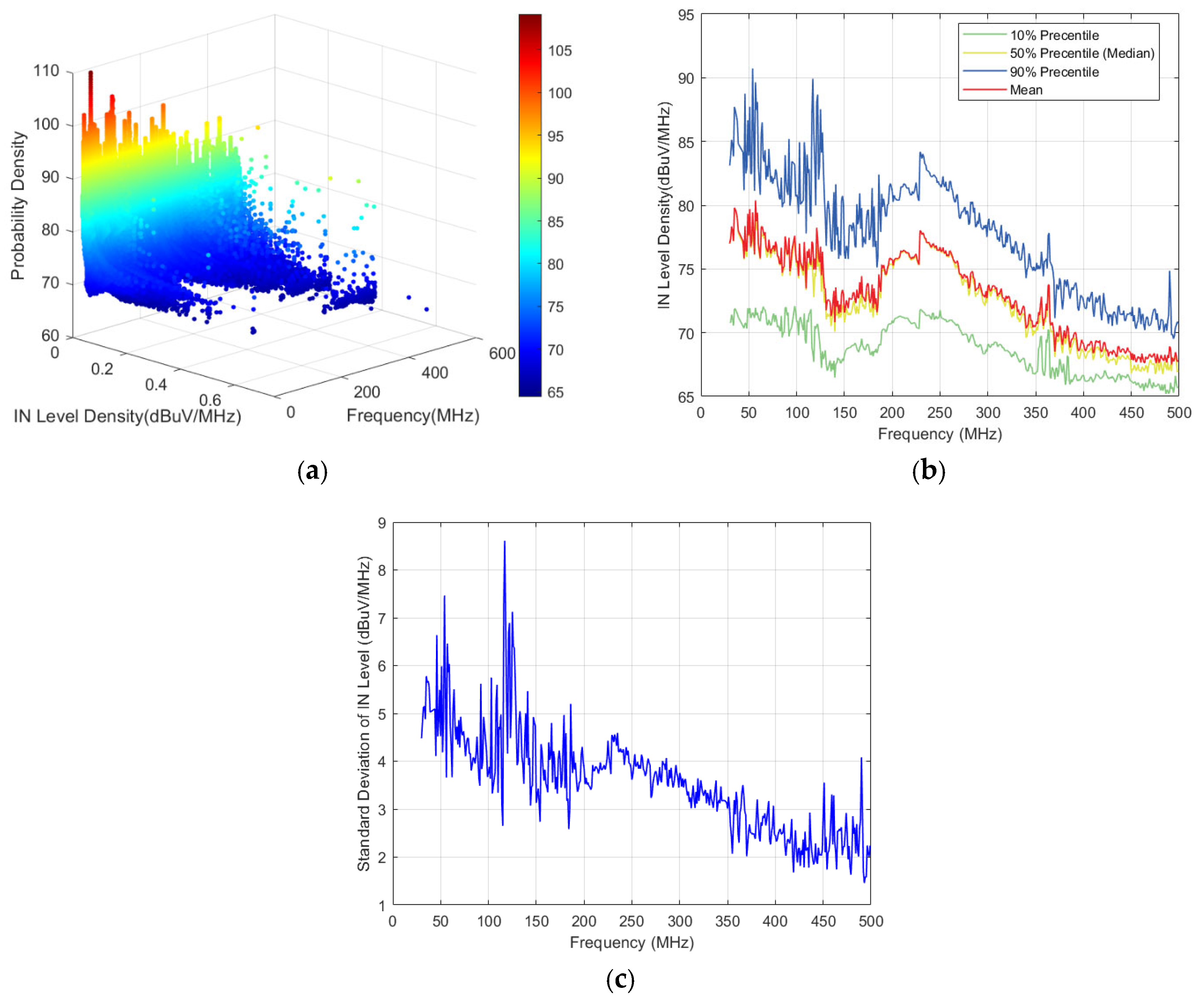
The calculation results of the impulse level density component are shown in Figure 13a. The probability density represents the proportion of different IN level densities observed in a single measurement. Figure 13b and Figure 13c illustrate the statistical distribution and variance of the IN level density at each frequency, respectively.

Figure 13. Statistical analysis of IN level density: (a) IN level density. (b) Statistical distribution of the IN level density. (c) Variance of the IN level density.

Calculate the pulse length as

T_IN = N_IN / f_s

(13)

where N_IN is the number of samples between pulse start and end. f_s is sampling frequency (Hz).

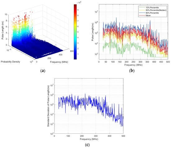
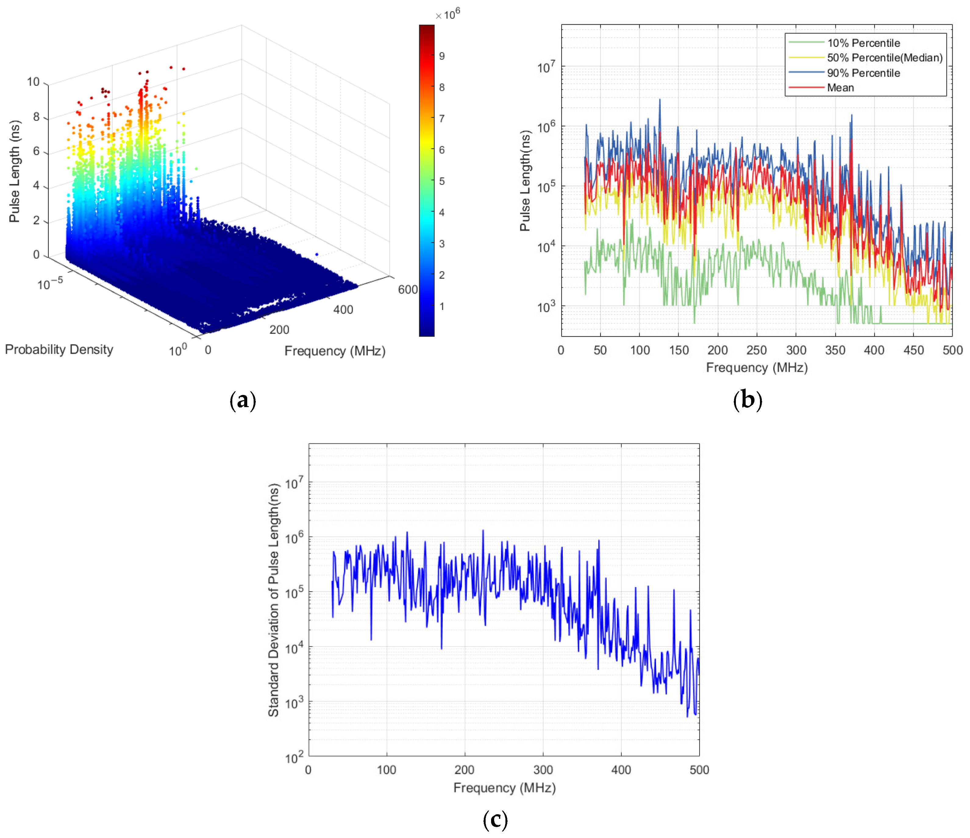
The statistical results of the pulse length of the measured samples are shown in Figure 14a. Figure 14b and Figure 14c illustrate the statistical distribution and variance of the pulse length at each frequency, respectively.

Figure 14. Statistical analysis of pulse length: (a) Pulse length within 30–500 MHz. (b) Statistical distribution of the pulse length. (c) Variance of the pulse length.

The following conclusions can be drawn from the above figures.

The frequency distribution characteristics of pulse occurrences are evident. Pulse events are primarily concentrated in the 30–140 MHz and 200–270 MHz frequency bands, indicating that pulse activity is most pronounced within these ranges.

Pulse levels exhibit a declining trend with increasing frequency, and the distribution of high-level pulses shows distinct frequency band characteristics. The maximum density of pulse levels generally decreases as frequency rises, diminishing from approximately 115 dBμV/Hz to 95 dBμV/Hz. Among these, high-level pulses are mainly concentrated in the 100–200 MHz and 400–500 MHz bands, yet they constitute only a minor proportion at each frequency; in contrast, low-level pulses in the 60–80 dBμV range dominate the majority, forming the primary component of pulse events.

The roll-off of the maximum IN level density above 270 MHz is primarily attributed to the intrinsic spectral characteristics of the man-made noise sources at the mountainous observation station. The dominant sources, such as power transmission lines, lighting equipment, and vehicle engines, radiate predominantly in the HF/VHF bands below 200 MHz, with harmonic amplitudes decaying rapidly at higher frequencies. While antenna efficiency, path loss, and receiver sensitivity may contribute to a lesser extent, they are not considered the dominant factors.

Wide pulses account for an extremely low proportion of the overall pulses. Pulses with widths greater than 0.001 s are distributed across the 30–400 MHz frequency band, but their proportion at each frequency remains below 0.01%, suggesting that while wide pulses exhibit broad frequency distribution characteristics, they represent a negligible fraction of all pulse events.

It is worth noting that the impulsive noise exhibits distinct concentration in specific sub-bands, notably 30–140 MHz and 200–270 MHz. This frequency-band concentration suggests that automated digital excision filters could be a promising approach for suppressing impulsive noise in radio observation systems. Two possible strategies can be considered. First, a frequency-domain excision filter could be designed to attenuate the sub-bands where impulsive events are most concentrated, while preserving the sub-bands with lower impulsive activity. Second, a time-domain excision filter could be applied to detect and blank short-duration impulsive events based on an amplitude threshold, which is a common approach in impulsive noise mitigation. Since the impulsive events observed in this study are primarily concentrated at low levels (60–80 dBμV/Hz) and exhibit short durations, a threshold-based time-domain excision filter may be more suitable than a frequency-domain filter. However, the design of such filters requires careful consideration of the trade-off between noise suppression and signal distortion, especially for weak astronomical signals. Future work will investigate the feasibility of implementing automated digital excision filters based on the statistical characteristics of impulsive noise reported in this study.

5.2. Impulse Noise Modeling

Influenced by the distribution of environmental noise sources and their time-varying characteristics, the statistical properties of impulsive parameters rarely exhibit consistent distributions or patterns. Describing these parameters using a single or a combination of statistical distributions proves to be inaccurate. Therefore, this article employs the XGBoost decision tree algorithm to model the impulsive parameter features and to perform data training and prediction, rather than relying on traditional distribution-based modeling.

Prior to training the XGBoost models, the input features were selected based on their impact on prediction accuracy. For IN level density, frequency, mean, and probability density had the most significant impact. For pulse length, the raw data exhibited a wide dynamic range (500 ns to 10⁷ ns) and a skewed distribution heavily concentrated at lower values. A natural logarithmic transformation was therefore applied to compress the variation range and enhance learning stability. After training, the predictions were inverse-transformed back to the original space for evaluation. The analysis revealed that frequency, mean, RMSE, and probability density were the most influential predictors for the log-transformed pulse length.

The hyperparameters of the XGBoost model were configured as follows: the learning rate was set to 0.005, the maximum tree depth to 8, and the feature subsampling rate to 0.8. Additionally, both the L1 and L2 regularization weights were set to 0.1. These parameter values were determined through empirical tuning.

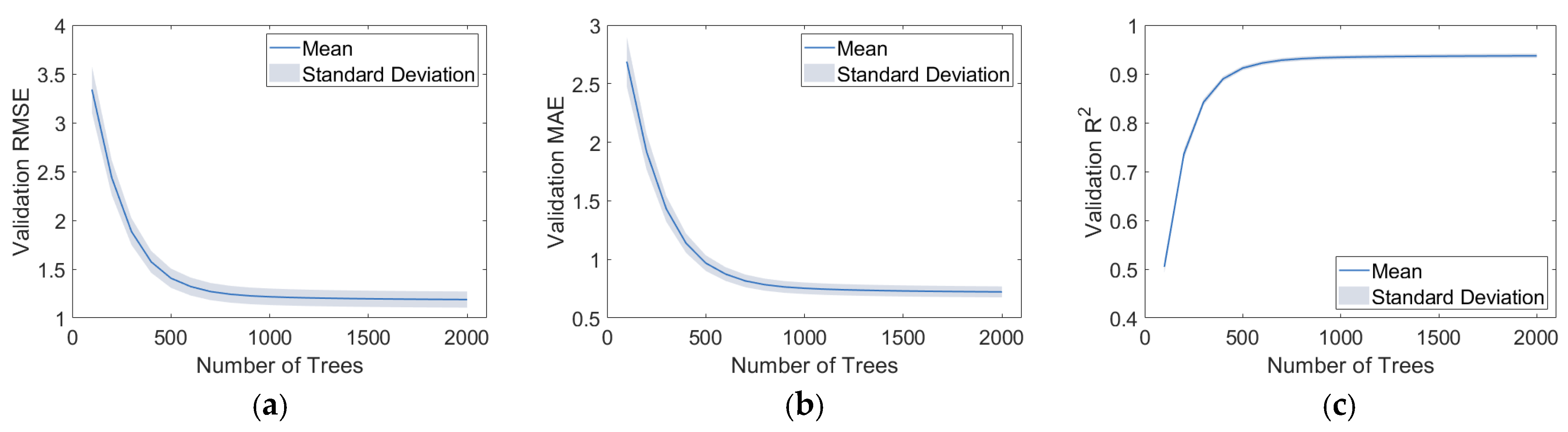
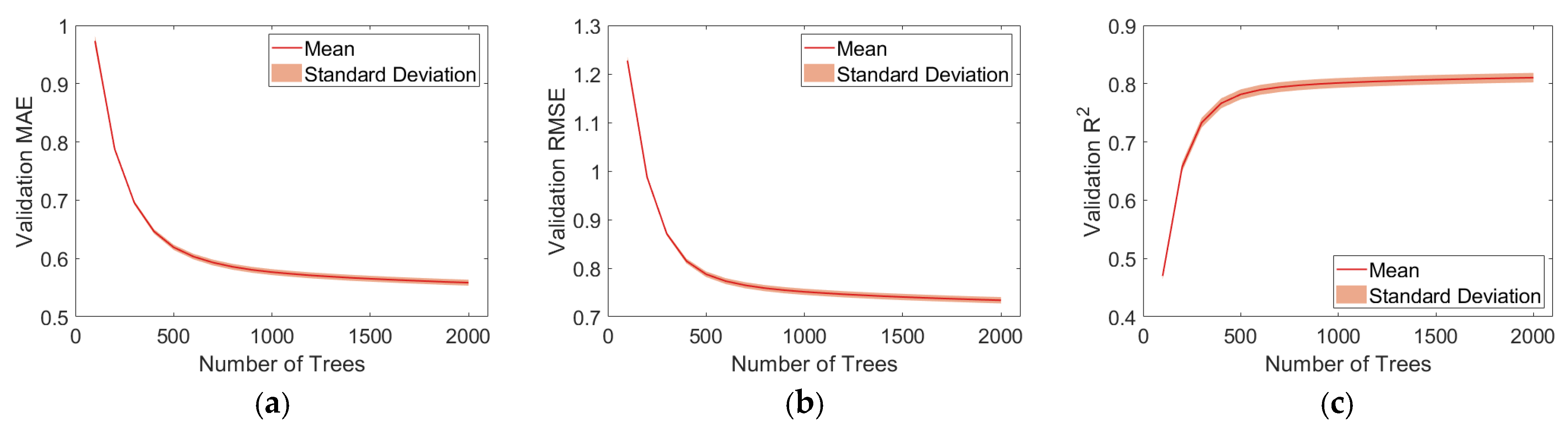
To determine the optimal number of boosting rounds without biasing the final evaluation, the data were first partitioned into six consecutive 4 h time blocks according to their acquisition order within each frequency. A leave-one-time-block-out cross-validation was then employed. In each fold, one time block was held out as the validation set, while the remaining five blocks were used for training. The number of trees was varied from 100 to 2000 in steps of 100, and the validation RMSE, MAE, and R² were recorded at each step. The average validation metrics across the six folds were used to select the globally optimal number of trees.

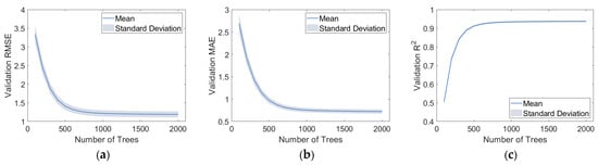
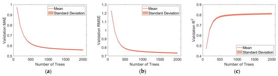
As shown in Figure 15 and Figure 16, for IN level density, the validation RMSE decreased rapidly from 3.3398 ± 0.2384 at 100 trees to 1.4071 ± 0.0985 at 500 trees, and then gradually approached 1.1884 ± 0.0830 at 2000 trees. The diminishing returns beyond 500 trees indicate that the model has largely converged. The standard deviation across the six folds remained stable at approximately 0.08 throughout, indicating consistent convergence behavior across different time periods. For pulse length, the validation RMSE decreased rapidly from 1.2273 ± 0.0093 at 100 trees to 0.7875 ± 0.0058 at 500 trees, and then gradually approached 0.7339 ± 0.0066 at 2000 trees. Similarly, the diminishing returns beyond 500 trees indicate that the model has largely converged, and the standard deviation across the six folds remained stable at approximately 0.0065 throughout.

Figure 15. Validation indicators of IN Level Density under different tree quantities: (a) RMSE; (b) MAE; (c) R².

Figure 16. Validation indicators of Pulse Length under different tree quantities: (a) RMSE; (b) MAE; (c) R².

Considering both prediction accuracy and computational efficiency, 1500 trees were selected as the number of boosting rounds for the XGBoost models of both IN Level Density and Pulse Length.

In the second stage, the model was re-trained with the optimal number of trees, 1500, and evaluated using the same cross-validation. For each fold, one time block was held out as the test set, and the remaining five blocks were used for training and validation, with 20% of the training data randomly reserved as the validation set for monitoring. Importantly, the test set was never used during hyperparameter selection, ensuring that the reported performance is not optimistically biased.

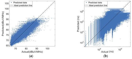
For IN level density, the results are shown in Figure 17a and Table 4. The model achieved an average validation R² of 0.9372 ± 0.0045, demonstrating stable performance across all folds. The test R² varied considerably, ranging from 0.6618 to 0.9276, with an average of 0.8191 ± 0.0934. The lowest R² occurred during the early morning transition period (4:00–8:00), where the radio noise characteristics differ from those of the adjacent time blocks. In contrast, the afternoon and evening periods (12:00–20:00) showed more consistent patterns, allowing the model to achieve R² values above 0.90.

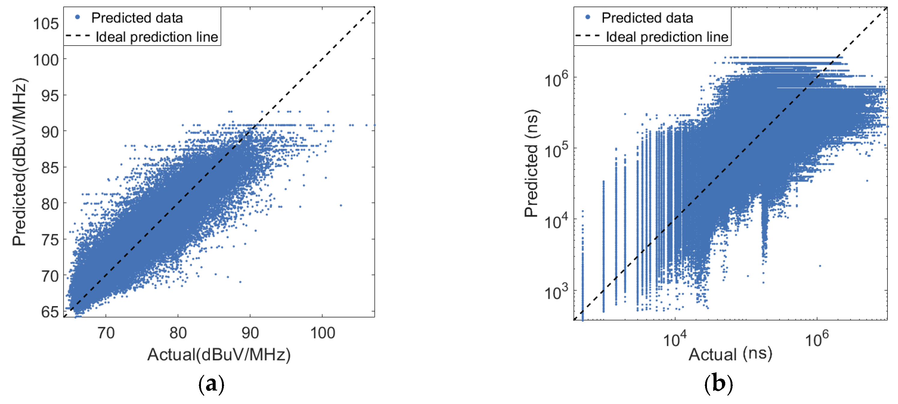
Figure 17. The actual and predicted values: (a) IN level density; (b) pulse length.

Table 4. Cross-validation results for IN level density.

Fold	Test Block	Verification RMSE	Verification MAE	Verification R2	Test RMSE	Test MAE	Test R2
1	Block 1	1.2329	0.7613	0.9343	3.5490	2.5917	0.7712
2	Block 2	1.2092	0.7510	0.9414	1.4809	1.0062	0.6618
3	Block 3	1.2165	0.7377	0.9412	1.3921	0.9473	0.8226
4	Block 4	1.2299	0.7322	0.9367	1.2581	0.8833	0.9061
5	Block 5	1.2220	0.7221	0.9298	1.3289	0.9216	0.9276
6	Block 6	1.0199	0.6308	0.9396	2.4090	1.7882	0.8253
Mean	—	1.1884 ± 0.0830	0.7225 ± 0.0470	0.9372 ± 0.0045	1.9030 ± 0.9110	1.3564 ± 0.6950	0.8191 ± 0.0934

For pulse length, the results are shown in Figure 17b and Table 5. The model achieved an average validation R² of 0.8103 ± 0.0082. The test R² ranged from 0.6844 to 0.8145, with an average of 0.7534 ± 0.0503. Unlike the IN level density model, the lowest test performance occurred during the morning period (8:00–12:00), while the highest was observed at night (20:00–24:00). The different temporal patterns observed for IN level density and pulse length can be attributed to their distinct physical origins. IN Level Density is primarily governed by the strength of local noise sources, which follows the diurnal cycle of human activity and electrical load. In contrast, pulse length is more closely related to the duration of specific impulsive events, such as switching operations or engine ignition, which may peak at different times of day. Consequently, the periods of lowest model performance differ between the two prediction targets.

Table 5. Cross-validation results for pulse length.

Fold	Test Block	Verification RMSE	Verification MAE	Verification R2	Test RMSE	Test MAE	Test R2
1	Block 1	0.7371	0.5616	0.8065	0.7789	0.5864	0.7934
2	Block 2	0.7262	0.5528	0.8179	0.8613	0.6607	0.7122
3	Block 3	0.7255	0.5520	0.8203	0.8686	0.6724	0.6844
4	Block 4	0.7357	0.5580	0.8112	0.8215	0.6389	0.7375
5	Block 5	0.7377	0.5622	0.8083	0.8070	0.6111	0.7784
6	Block 6	0.7415	0.5643	0.7978	0.7921	0.5990	0.8145
Mean	—	0.7339 ± 0.0066	0.5585 ± 0.0051	0.8103 ± 0.0082	0.8216 ± 0.0366	0.6281 ± 0.0347	0.7534 ± 0.0503

To evaluate whether the proposed XGBoost model is truly necessary, three baseline methods were implemented, including linear regression, polynomial regression with degrees 2 and 3, and random forest. For pulse length prediction, the same natural-log transformation was applied to the target variable before training all baseline models, and the predicted values were inverse-transformed back to the original space for evaluation. Their performance was compared with the proposed XGBoost model under the same data partitioning scheme for both IN level density and pulse length prediction.

Table 6 shows the comparison of different models for IN level density prediction. The linear regression model achieved the lowest performance, with a validation R² of 0.4614 and a test R² of only 0.0883, indicating that the relationship between the input features and the IN level density is highly nonlinear. Polynomial regression with degree 2 improved the validation R² to 0.5811 and the test R² to 0.1970, while degree 3 further improved them to 0.6510 and 0.2056, respectively. However, both polynomial models still exhibited limited predictive capability, suggesting that a simple polynomial form cannot adequately capture the complex nonlinearity of the data. The random forest model achieved a validation R² of 0.8469 and a test R² of 0.6265, outperforming the linear and polynomial models by a considerable margin, which confirms the advantage of ensemble tree-based methods for this task. Nevertheless, the proposed XGBoost model achieved the best performance, with a validation R² of 0.9372 and a test R² of 0.8191.

Table 6. Comparison of the proposed XGBoost model with baseline methods for IN level density prediction.

Model	Verification RMSE	Verification MAE	Verification R2	Test RMSE	Test MAE	Test R2
Linear Regression	3.6244	3.0161	0.4614	5.5031	4.5923	0.0883
Polynomial (deg = 2)	3.1961	2.6563	0.5811	5.1646	4.2303	0.1970
Polynomial (deg = 3)	2.9176	2.4078	0.6510	5.1371	3.9788	0.2056
Random Forest	1.9325	1.4930	0.8469	3.5226	2.9915	0.6265
XGBoost	1.1884	0.7225	0.9372	1.9030	1.3564	0.8191

Table 7 shows the comparison of different models for pulse length prediction. Linear regression obtained a validation R² of 0.3332 and a test R² of 0.3436. Polynomial regression with degree 2 improved the validation R² to 0.4918 and the test R² to 0.5305, while degree 3 further improved them to 0.5401 and 0.5877, respectively. The random forest model achieved a validation R² of 0.7075 and a test R² of 0.7320, clearly outperforming the linear and polynomial models. XGBoost achieved the highest test R² of 0.7534, slightly outperforming the random forest model (0.7320) and clearly outperforming the linear and polynomial models.

Table 7. Comparison of the proposed XGBoost model with baseline methods for pulse length prediction.

Model	Verification RMSE	Verification MAE	Verification R2	Test RMSE	Test MAE	Test R2
Linear Regression	1.3999	1.1342	0.3332	1.4899	1.2104	0.3436
Polynomial (deg = 2)	1.2221	0.9844	0.4918	1.2601	1.0056	0.5305
Polynomial (deg = 3)	1.1626	0.9278	0.5401	1.1809	0.9286	0.5877
Random Forest	0.9271	0.6965	0.7075	0.8780	0.6524	0.7320
XGBoost	0.7339	0.5585	0.8103	0.8216	0.6281	0.7534

Comparing the two targets, the proposed XGBoost model consistently outperformed all baseline methods for both IN level density and pulse length prediction. For impulse level density, XGBoost improved the test R² from 0.6265 to 0.8191 compared with the strongest baseline, corresponding to a relative improvement of approximately 31%. For pulse length, XGBoost achieved the highest test R² of 0.7534, slightly outperforming the random forest model (0.7320) and clearly outperforming the linear and polynomial models. These results confirm that the proposed XGBoost model is far more accurate than conventional linear, polynomial, and random forest models for both prediction tasks. The consistent superiority of XGBoost across both targets demonstrates its robustness and effectiveness for radio noise parameter prediction in mountainous observation stations.

It should be noted that the input features used in the proposed XGBoost models are all statistical features derived from the measured radio noise data, including frequency, mean, RMSE, and probability density. Contextual variables such as time of day, weather conditions, and telemetry from the observatory’s electrical grid were not incorporated in the current study. While time-of-day information is implicitly captured by the time-block-based cross-validation procedure, the absence of weather and electrical grid telemetry limits the model’s ability to distinguish between external environmental pulses and intra-site switching transients. Future work will consider incorporating these contextual variables to further improve the model’s predictive capability and source attribution.

6. Conclusions

This article presents a radio noise measurement campaign conducted at an observation station in a mountainous area. Based on the analysis and modeling of both Gaussian and impulsive components, several key conclusions are drawn. First, the preprocessing procedures for the raw data are described. Subsequently, the noise figure, representing the Gaussian component within the 30–500 MHz frequency range, was calculated. These results were compared with the ITU-R P.372-17 human-made radio noise model, and the median noise figure was modeled using smoothing spline regression. The results indicate that the noise figure decreases as frequency increases. However, the measured values are significantly higher than the reference levels for various areas specified in the ITU-R P.372-17 model. Furthermore, the smoothing spline model demonstrated significantly higher accuracy compared to log-linear regression methods.

Regarding the impulsive component, impulse signals were first extracted and merged from the raw data. Three key statistical parameters—total impulse length, IN level density, and pulse length—were analyzed. Instead of relying on typical statistical distributions, the XGBoost algorithm was employed to predict these parameters. The analysis reveals that impulse occurrences are primarily concentrated within specific frequency bands, with both impulse amplitude and pulse length decreasing as frequency increases. Moreover, the XGBoost decision tree model exhibited robust accuracy in predicting these parameters. The findings of this study provide valuable guidance for the deployment of radio services at mountainous observation stations.

However, several limitations should be acknowledged. The measurement campaign was conducted over a total duration of only 24 h, which may not fully capture the temporal variability of radio noise. Radio noise conditions can vary significantly with time of day, weather, human activity, equipment operation, and other environmental factors. Consequently, the models derived from a single measurement period should not be over-generalized to other mountainous radio observatories or different environmental conditions without caution. Future work should include measurements over additional days and under diverse environmental conditions to improve the representativeness and generalization capability of the proposed models.

References

- ITU-R SM.1753-2; Methods for Measurements of Radio Noise. ITU: Geneva, Switzerland, 2012.
- ITU-R P.372-17; Radio Noise. ITU: Geneva, Switzerland, 2023.
- Sorecau, E.; Sorecau, M.; Craiu, N.; Sarbu, A.; Bechet, P. Man-made Noise Measurement System for HF Band Based on SDR platforms—Design and Implementation. In Proceedings of the 2022 International Symposium on Electronics and Telecommunications (ISETC), Timisoara, Romania, 10–11 November 2022; pp. 1–4. [Google Scholar] [CrossRef] [Scilit]
- Leferink, F.; Silva, F.; Catrysse, J.; Batterman, S.; Beauvois, V.; Roc’h, A. Man-made noise in our living environments. URSI Radio Sci. Bull. 2010, 2010, 49–57. [Google Scholar] [CrossRef]
- Bechet, P.; Bechet, A.C.; Miclaus, S. HF urban noise level in variable channels of 3–24 kHz: A preliminary experimental approach. In Proceedings of the Loughborough Antennas & Propagation Conference; IET: Loughborough, UK, 2017. [Google Scholar]
- Fockens, T.W.H.; Zwamborn, A.P.M.; Leferink, F. Measurement Methodology and Results of Measurements of the Man-Made Noise Floor on HF in The Netherlands. IEEE Trans. Electromagn. Compat. 2019, 61, 337–343. [Google Scholar] [CrossRef] [Scilit]
- Popescu, O.; Musson, J.; Popescu, D.C. Using Open-Source Software Defined Radio Platforms for Empirical Characterization of Man-Made Impulsive Noise. IEEE Electromagn. Compat. Mag. 2020, 9, 54–61. [Google Scholar] [CrossRef] [Scilit]
- Fockens, K.T.; Leferink, F. Correlation Between Measured Man-Made Noise Levels and the Density of Habitation. IEEE Trans. Electromagn. Compat. 2020, 62, 2696–2703. [Google Scholar] [CrossRef] [Scilit]
- Haedrich, C.E.; Wilson, D.K.; Breton, D.J. Isarithmic Mapping of Radio-Frequency Noise in the Urban Environment; Tech. Rep. ERDC/CRREL MP-20-12; Engineer Research and Development Center: Hanover, MA, USA, 2020. [Google Scholar] [CrossRef] [Scilit]
- Sitompul, P.P.; Manik, T.; Batubara, M.; Suhandi, B. Radio Frequency Interference Measurements for a Radio Astronomy Observatory Site in Indonesia. Aerospace 2021, 8, 51. [Google Scholar] [CrossRef] [Scilit]
- Küçük, İ.; Üler, I.; Öz, Ş.; Onay, S.; Özdemir, A.R.; Gülşen, M.; Sarıkaya, M.; Dagtekin, N.D.; Özeren, F.F. Site selection for a radio astronomy observatory in Turkey: Atmospheric, meteorological, and radio frequency analyses. Exp. Astron. 2012, 33, 1–26. [Google Scholar] [CrossRef] [Scilit]
- Abidin, Z.Z.; Adnan, S.; Ibrahim, Z.A. RFI profiles of prime candidate sites for the first radio astronomical telescope in Malaysia. New Astron. 2010, 15, 307–312. [Google Scholar] [CrossRef] [Scilit]
- Gulati, K.; Evans, B.L.; Andrews, J.G.; Tinsley, K.R. Statistics of co-channel interference in a field of Poisson and Poisson-Poisson clustered interferes. IEEE Trans. Signal Process. 2010, 58, 6207–6222. [Google Scholar] [CrossRef] [Scilit]
- Soussen, C.; Idier, J.; Brie, D.; Duan, J. From Bernoulli–Gaussian Deconvolution to Sparse Signal Restoration. IEEE Trans. Signal Process. 2011, 59, 4572–4584. [Google Scholar] [CrossRef] [Scilit]
- Middleton, D. Non-Gaussian noise models in signal processing for telecommunications: New methods an results for class A and class B noise models. IEEE Trans. Inf. Theory 1999, 45, 1129–1149. [Google Scholar] [CrossRef] [Scilit]
- Georgiou, P.G.; Tsakalides, P.; Kyriakakis, C. Alpha-stable modeling of noise and robust time-delay estimation in the presence of impulsive noise. IEEE Trans. Multimed. 1999, 1, 291–301. [Google Scholar] [CrossRef] [Scilit]
- Ilow, J.; Hatzinakos, D. Analytic alpha-stable noise modeling in a Poisson field of interferers or scatterers. IEEE Trans. Signal Process. 1998, 46, 1601–1611. [Google Scholar] [CrossRef] [Scilit]
- Rouissi, F.; Vinck, A.J.H.; Gassara, H.; Ghazel, A. Improved impulse noise modeling for indoor narrow-band power line communication. AEU—Int. J. Electron. Commun. 2019, 103, 74–81. [Google Scholar] [CrossRef] [Scilit]
- Landa, I.; Diez-Bravo, A.; Velez, M.; Arrinda, A. Influence of impulsive noise from lifts on orthogonal frequency-division multiplexing digital radio mondiale signals. IET Commun. 2020, 14, 111–116. [Google Scholar] [CrossRef] [Scilit]
- Rouissi, F.; Vinck, A.J.H.; Ghazel, A. On the simulation of the Middleton Class-A noise model for single- and multi-carrier modulation in power line communication. Telecommun. Syst. 2021, 77, 143–153. [Google Scholar] [CrossRef] [Scilit]
- Ndo, G.; Labeau, F.; Kassouf, M. A Markov-Middleton Model for Bursty Impulsive Noise: Modeling and Receiver Design. IEEE Trans. Power Deliv. 2013, 28, 2317–2325. [Google Scholar] [CrossRef] [Scilit]
- Sanchez, M.G.; de Haro, L.; Ramon, M.C.; Mansilla, A.; Ortega, C.M.; Oliver, D. Impulsive noise measurements and characterization in a UHF digital TV channel. IEEE Trans. Electromagn. Compat. 1999, 41, 124–136. [Google Scholar] [CrossRef]
- Zhang, J.; Liu, L.; Wang, K. Measurements and statistical analyses of electromagnetic noise for industrial wireless communications. Int. J. Intell. Syst. 2021, 36, 1716–1740. [Google Scholar] [CrossRef] [Scilit]
- Chen, T.; Guestrin, C. Xgboost: A scalable tree boosting system. In Proceedings of the 22nd ACM SIGKDD International Conference on Knowledge Discovery and Data Mining, San Francisco, CA, USA, 13–17 August 2016; pp. 785–794. [Google Scholar]
- Chen, W.; Fu, K.; Zuo, J.; Zheng, X. Radar emitter classification for large data set based on weighted-xgboost. IET Radar Sonar Navig. 2017, 11, 1203–1209. [Google Scholar] [CrossRef] [Scilit]
- Zhou, S. Gwo-ga-xgboost-based model for Radio-Frequency power amplifier under different temperatures. Expert Syst. Appl. 2025, 278, 127439. [Google Scholar] [CrossRef] [Scilit]
- Liu, Y.; Liu, L.; Yang, L.; Hao, L.; Bao, Y. Measuring distance using ultra-wideband radio technology enhanced by extreme gradient boosting decision tree (XGBoost). Autom. Constr. 2021, 126, 103678. [Google Scholar] [CrossRef] [Scilit]
- Rekkas, V.; Sotiroudis, S.P.; Zaharis, Z.D. Machine Learning-Based Radio Environment Maps for 4G/5G Networks. IEEE Trans. Antennas Propag. 2025, 73, 10529–10543. [Google Scholar] [CrossRef] [Scilit]
- Feng, Y.; Liu, L.; Shu, J. A Link Quality Prediction Method for Wireless Sensor Networks Based on XGBoost. IEEE Access 2019, 7, 155229–155241. [Google Scholar] [CrossRef] [Scilit]
Disclaimer/Publisher’s Note: The statements, opinions and data contained in all publications are solely those of the individual author(s) and contributor(s) and not of MDPI and/or the editor(s). MDPI and/or the editor(s) disclaim responsibility for any injury to people or property resulting from any ideas, methods, instructions or products referred to in the content. |
© 2026 by the authors. Licensee MDPI, Basel, Switzerland. This article is an open access article distributed under the terms and conditions of the Creative Commons Attribution (CC BY) license.