STG-Mixer: A Multi-Region, Multi-Step Forecasting Network for Hand, Foot, and Mouth Disease with Multi-Timescale Feature Extraction and Spatial Association Learning

Abstract

Accurate forecasting of hand, foot, and mouth disease (HFMD) incidence is crucial for effective prevention and control. However, existing multi-region HFMD forecasting models remain limited in jointly capturing multi-timescale temporal patterns and interregional spatial associations, which affects multi-step forecasting performance. In this study, we propose Spatiotemporal Graph Mixer (STG-Mixer), a multi-region, multi-step forecasting network for HFMD based on multi-timescale feature extraction and spatial association learning. STG-Mixer constructs a graph structure based on interregional adjacency relationships and adopts a dual-branch spatiotemporal encoder consisting of an Adaptive Fusion Spatial Branch (AF-SB) and a Multi-Scale Energy-Gated Temporal Branch (MEG-TB). Specifically, AF-SB employs a dual-layer Temporal Graph Convolutional Network (T-GCN), TimeKAN block, and Orthogonal Residual Gated Fusion mechanism to learn spatial representations, while MEG-TB extracts and adaptively weights temporal features across multiple scales using dilated temporal convolutions and an energy-gated mechanism. The learned spatial and temporal representations are fused and fed into an autoregressive decoder for multi-step forecasting. Experiments on HFMD surveillance and meteorological data from 47 prefectures in Japan demonstrate that STG-Mixer outperforms baseline models in one- to four-week-ahead forecasting. Additional experiments on an independent HFMD dataset from southern China further evaluate the forecasting capability of the proposed model under a different temporal resolution.

1. Introduction

Hand, foot, and mouth disease (HFMD) is a common infectious disease that primarily affects preschool children and poses a substantial public health burden, particularly in the Asia-Pacific region [1,2,3,4]. HFMD incidence exhibits significant seasonal fluctuations and regional heterogeneity [5,6,7], making accurate forecasting essential for epidemic surveillance, prevention planning, and public health resource allocation. However, the complex interactions among temporal variations, spatial dependencies, and environmental factors make multi-region and multi-step HFMD forecasting a challenging task.

A variety of statistical time-series approaches have been applied to HFMD forecasting. Autoregressive integrated moving average (ARIMA) models have been used to characterize temporal trends and seasonal variations in HFMD incidence [8]. Meteorological variables, including temperature and humidity, have also been incorporated into regression-based frameworks to investigate their associations with HFMD transmission [9]. Exponential smoothing state-space models have been adopted to capture seasonal characteristics [10], while recent studies have compared seasonal autoregressive integrated moving average (SARIMA) and Prophet-based approaches for HFMD forecasting [11]. Epidemiological studies have further demonstrated that meteorological conditions may exhibit delayed and nonlinear associations with HFMD incidence [12,13]. Although these statistical approaches provide valuable interpretability, they generally rely on predefined assumptions and have limited capability in modeling complex nonlinear interactions among multiple epidemiological and environmental factors.

Machine learning methods have subsequently been introduced to improve the representation of nonlinear relationships in HFMD forecasting. Random forest and XGBoost models have been employed to integrate epidemiological and meteorological variables for HFMD prediction [14], while support vector regression has also been applied with meteorological covariates [15]. Hybrid approaches combining optimization algorithms and neural networks have been explored for disease prediction and early warning [16]. More recently, Bayesian additive regression trees have been utilized to provide probabilistic HFMD forecasts with prediction intervals [17]. These studies demonstrate that incorporating multiple explanatory variables can improve forecasting performance [18]. However, many machine learning-based approaches remain focused on short-term or single-step prediction, and maintaining stable forecasting performance over longer prediction horizons remains challenging.

Deep learning approaches provide enhanced capability for modeling complex temporal and spatiotemporal dependencies in time-series data [19]. Long short-term memory (LSTM) networks have been applied to HFMD incidence forecasting by learning short- and long-term temporal dependencies from historical surveillance sequences [20]. Time-series decomposition and feature-fusion strategies have also been introduced to separately model trend and seasonal components [21]. Multi-input multi-output frameworks have further enabled multi-step HFMD forecasting by incorporating epidemiological and meteorological information with different temporal lags [22]. In addition, causal convolutional neural networks have been explored to analyze temporal relationships between meteorological factors and HFMD incidence [23]. Although these deep learning approaches improve temporal feature extraction, they mainly focus on temporal patterns and may not fully capture spatial dependencies among different regions.

Recently, graph-based spatiotemporal forecasting methods have provided an effective framework for modeling complex spatial and temporal dependencies [24], and such approaches are increasingly relevant to regional infectious disease forecasting. Graph neural networks (GNNs) represent regions as nodes and their relationships as edges, enabling the learning of spatial correlations among different locations. Temporal Graph Convolutional Networks (T-GCNs) combine graph convolution and recurrent networks to jointly capture spatial and temporal dependencies and have been widely applied in spatiotemporal forecasting tasks [25]. Graph-based approaches have also been introduced into HFMD prediction to encode spatial relationships among regions and improve spatiotemporal representation learning [26]. Deng et al. [27] proposed Cola-GNN for long-term influenza-like illness prediction, demonstrating the application of cross-location attention and graph neural networks to regional epidemic forecasting. Lozano et al. [28] developed a deep learning-based COVID-19 forecasting framework alongside intervention-strategy optimization, providing further methodological context for data-driven epidemic prediction. Furthermore, attention-based and multi-horizon forecasting architectures have demonstrated promising performance in modeling complex spatiotemporal and long-range temporal dependencies [29,30,31,32]. Nevertheless, effectively integrating interregional spatial associations with temporal patterns at multiple scales remains challenging for multi-region, multi-step HFMD forecasting.

To address these challenges, we propose the Spatiotemporal Graph Mixer (STG-Mixer), a multi-region, multi-step forecasting network for HFMD based on multi-timescale feature extraction and spatial association learning. STG-Mixer consists of an Adaptive Fusion Spatial Branch (AF-SB) and a Multi-Scale Energy-Gated Temporal Branch (MEG-TB). The AF-SB learns interregional spatial representations through graph-based aggregation, nonlinear spatial transformation, and adaptive feature fusion, while the MEG-TB captures informative temporal patterns across multiple scales through dilated temporal convolutions and an energy-gated mechanism. The learned spatial and temporal representations are integrated and fed into an autoregressive decoder to generate multi-step HFMD forecasts.

The main contributions of this study are summarized as follows:

(1)

We propose STG-Mixer, a novel multi-region, multi-step HFMD forecasting model that jointly captures spatial associations among cases across regions and temporal relationships between meteorological variables and HFMD incidence, thereby improving the accuracy and stability of multi-region forecasting.

(2)

We design the Adaptive Fusion Spatial Branch (AF-SB), which propagates and aggregates HFMD case information from neighboring regions through a dual-layer T-GCN aggregation block. A TimeKAN block is further introduced to enhance the modeling of complex nonlinear spatial dependencies, while the Orthogonal Residual Gated Fusion mechanism integrates projection-based residual features through adaptive gating to improve forecasting performance.

(3)

We construct the Multi-Scale Energy-Gated Temporal Branch (MEG-TB), which captures multi-timescale temporal features from HFMD case data and meteorological variables through dilated temporal convolutions. An energy-gated mechanism is further employed to adaptively fuse features at different temporal scales and highlight information that is most relevant for prediction.

(4)

We conduct systematic comparative experiments and ablation studies on real-world HFMD surveillance data from 47 prefectures in Japan. The results demonstrate that STG-Mixer consistently outperforms the baseline models in one- to four-week-ahead forecasting tasks, and the ablation results further verify the effectiveness of the proposed components. Additional experiments on an independent HFMD dataset from a city in southern China further evaluate the forecasting capability of the proposed model under a different temporal resolution and provide external validation using an independent surveillance dataset.

2. Materials and Methods

2.1. Problem Formulation

This study formulates HFMD forecasting as a multi-region, multi-step spatiotemporal prediction problem using historical disease surveillance, meteorological, temporal, and geographical information. The regions within the study area and their geographical relationships are represented as an undirected graph $\mathcal{G}=(\mathcal{V},\mathcal{E})$, where $\mathcal{V}$ denotes the set of regional nodes and $\mathcal{E}$ represents the geographical connections between regions. The corresponding adjacency matrix is denoted by $\mathbf{A}\in {\mathbb{R}}^{N\times N}$, where N is the number of regions. The original spatial adjacency matrix is binary rather than weighted. Specifically, geographically adjacent regions are assigned a value of 1, whereas non-adjacent regions are assigned a value of 0, and no distance-based or other continuous edge weights are used. Before graph convolution, self-connections are introduced by adding an identity matrix to the original adjacency matrix. The resulting matrix is then symmetrically normalized using inverse-square-root node-degree scaling and subsequently used in the T-GCN for spatial feature aggregation.

A fixed geographical adjacency matrix was adopted because it directly represents persistent neighborhood relationships among prefectures and provides a stable spatial prior for interregional feature aggregation. In contrast, spatial relationships derived from short-term epidemiological or meteorological variations may fluctuate over time and may not consistently reflect stable interregional associations.

For each sample, observations from T consecutive time steps are used as the model input. The input tensor is represented as $\mathbf{X}\in {\mathbb{R}}^{B\times N\times F\times T}$, where B denotes the batch size, N is the number of regions, F is the number of input features for each region, and T is the length of the historical observation window. The input features include historical HFMD case counts, selected meteorological variables, and temporal sequence information.

Given a historical observation window of length T, the objective is to predict HFMD case counts for the subsequent L time steps across all target regions. The multi-step forecasting task can be expressed as

$${\widehat{\mathbf{Y}}}_{t+1},{\widehat{\mathbf{Y}}}_{t+2},\dots ,{\widehat{\mathbf{Y}}}_{t+L}=f\left(\mathcal{G};{\mathbf{X}}_{t-T+1},{\mathbf{X}}_{t-T+2},\dots ,{\mathbf{X}}_t\right),$$

(1)

where $f(·)$ denotes the forecasting model and ${\widehat{\mathbf{Y}}}_{t+l}$ represents the predicted HFMD case counts across all regions at the l-step-ahead horizon. In this study, experiments were conducted with $L\in \{1,2,3,4\}$ to evaluate forecasting performance over different prediction horizons.

2.2. Data Sources

Two HFMD datasets with different temporal resolutions and spatial settings were used in this study. The primary dataset consisted of prefecture-level HFMD surveillance data from Japan. Weekly HFMD case counts were obtained from the National Institute of Infectious Diseases (NIID), Japan, while the corresponding meteorological observations were obtained from the Japan Meteorological Agency (JMA).

The Japanese dataset covered the period from 2013 to 2023 and included weekly HFMD case counts from all 47 prefectures. The candidate meteorological variables included air temperature, relative humidity, atmospheric pressure, wind speed, and precipitation. In addition, a weekly sequence variable was constructed to represent annual seasonality. Geographical adjacency relationships among the 47 prefectures were used to construct the adjacency matrix for spatial modeling.

To further evaluate STG-Mixer under a different temporal resolution and spatial setting, an independent HFMD dataset from a city in southern China was used. This dataset was publicly released by the Chinese Center for Disease Control and Prevention and contained daily HFMD case records and meteorological observations from January 2014 to December 2019. Because this dataset contains only one region, the corresponding adjacency matrix reduces to a single-node self-connected graph.

2.3. Data Preprocessing and Feature Selection

For the Japanese dataset, all samples were first arranged chronologically and divided into training, validation, and test sets at a ratio of 7:1:2, corresponding to 2013 week 1–2020 week 36, 2020 week 37–2021 week 41, and 2021 week 42–2023 week 52, respectively. No missing observations were identified in the HFMD case-count series. In the meteorological records, 68 precipitation observations (0.0361%) and 46 relative-humidity observations (0.0244%) were missing, whereas no missing observations were found for temperature, atmospheric pressure, or wind speed. Missing meteorological values were handled using linear interpolation separately within each chronological data partition. Min–Max scaling parameters were estimated exclusively from the training set and were then applied unchanged to the validation and test sets. This procedure ensures that information from the validation and test periods is not used during model training. The weekly sequence variable was divided by 52 to represent annual seasonality.

For the Chinese dataset, all samples were arranged chronologically and divided into training and test sets at a ratio of 8:2, with the training partition covering 1 January 2014–18 October 2018 and the test partition covering 19 October 2018–31 December 2019. The dataset contained 365 missing observations, all of which occurred in the precipitation variable in 2019, accounting for 16.66% of the precipitation series. No missing observations were present in the HFMD case-count series; therefore, no imputed HFMD target values were included in the evaluation. Missing meteorological observations were handled using linear interpolation separately within the training and test partitions. The Min–Max scaling parameters were estimated exclusively from the training set and subsequently applied unchanged to the test set. The Chinese dataset was used as an independent external validation dataset to evaluate the forecasting capability of STG-Mixer under a different temporal resolution. For both datasets, chronological partitioning was performed before sliding-window sample construction, and samples were generated independently within each partition. Therefore, no input–target window crossed the boundaries between the training, validation, and test partitions.

The selection of candidate meteorological variables was informed by previous epidemiological evidence. Previous studies and meta-analyses have reported associations between HFMD incidence and meteorological factors including temperature, rainfall, relative humidity, and atmospheric pressure, and have also suggested that these associations may exhibit temporal lag effects [33]. Based on this evidence, the meteorological variables available in the Japanese dataset were included as candidate factors for further data-driven evaluation. Spearman’s rank correlation, a nonparametric measure of monotonic association [34], was first employed to examine their associations with HFMD incidence.

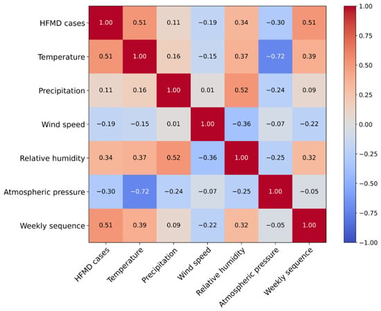
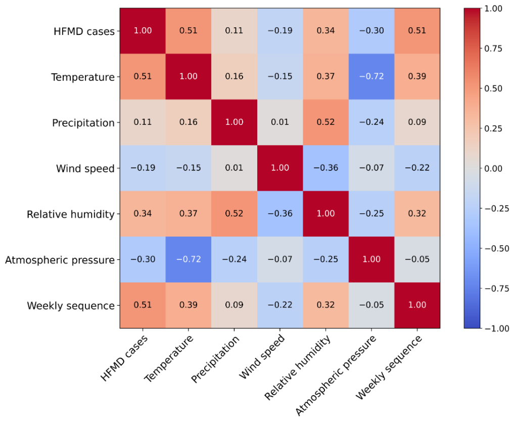
Spearman’s rank correlation analysis was performed using the training data to examine the associations between HFMD incidence and the candidate input variables, including air temperature, relative humidity, atmospheric pressure, wind speed, precipitation, and the weekly sequence variable. The correlations were first calculated separately for each of the 47 prefectures and then averaged across prefectures to obtain an overall correlation matrix, as shown in Figure 1.

Figure 1. Average Spearman correlation matrix between HFMD incidence and candidate input variables across the 47 prefectures of Japan, calculated using the training data.

To further examine potential delayed associations between meteorological factors and HFMD incidence, an additional lagged Spearman correlation analysis was conducted using only the training data. For each prefecture, meteorological observations at lags of 0–4 weeks were correlated with HFMD incidence at the corresponding future time point, and the resulting coefficients were averaged across the 47 prefectures. The analysis revealed distinct lag-dependent patterns across meteorological variables. In particular, the positive association of air temperature with HFMD incidence increased from 0.515 at lag 0 to 0.623 at lag 4, whereas atmospheric pressure exhibited an increasingly negative association from −0.297 to −0.455. Relative humidity showed a comparatively stable moderate positive association, while precipitation and wind speed exhibited weaker correlations. These results indicate that meteorological variables may be associated with HFMD incidence over different temporal lags and that contemporaneous correlation alone does not fully characterize these delayed relationships. The corresponding lagged correlation coefficients and mutual-information scores are summarized in Table 1.

Table 1. Mean lagged Spearman correlation coefficients and mutual-information scores between meteorological variables and HFMD incidence across the 47 prefectures of Japan using the training-period data.

Variable	Lag 0	Lag 1	Lag 2	Lag 3	Lag 4	MI
Air temperature	0.515	0.551	0.581	0.606	0.623	0.245
Precipitation	0.109	0.129	0.144	0.145	0.139	0.022
Wind speed	−0.191	−0.190	−0.178	−0.168	−0.145	0.044
Relative humidity	0.344	0.349	0.346	0.328	0.299	0.099
Atmospheric pressure	−0.297	−0.341	−0.387	−0.422	−0.455	0.123

To further complement the correlation-based analysis, mutual information was additionally calculated using only the training-period data to examine more general statistical dependencies between individual meteorological variables and HFMD incidence. Mutual information was estimated separately for each prefecture using a nearest-neighbor-based estimator [35], and the resulting scores were then averaged across the 47 prefectures. Air temperature showed the highest mean mutual-information score (0.245), followed by atmospheric pressure (0.123), relative humidity (0.099), wind speed (0.044), and precipitation (0.022). These results indicate that different association measures emphasize different aspects of the relationship between meteorological factors and HFMD incidence. Therefore, the final meteorological inputs were determined by jointly considering previous epidemiological evidence, contemporaneous and lagged Spearman correlation patterns, and complementary mutual-information analysis. Based on this combined evidence, air temperature, precipitation, and relative humidity were retained as meteorological input variables, together with the weekly sequence variable representing seasonal variation. The corresponding lagged Spearman correlation coefficients and mutual-information scores are summarized in Table 1.

2.4. STG-Mixer Model Architecture

2.4.1. Overall Architecture

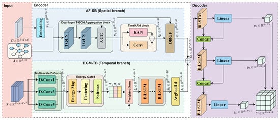
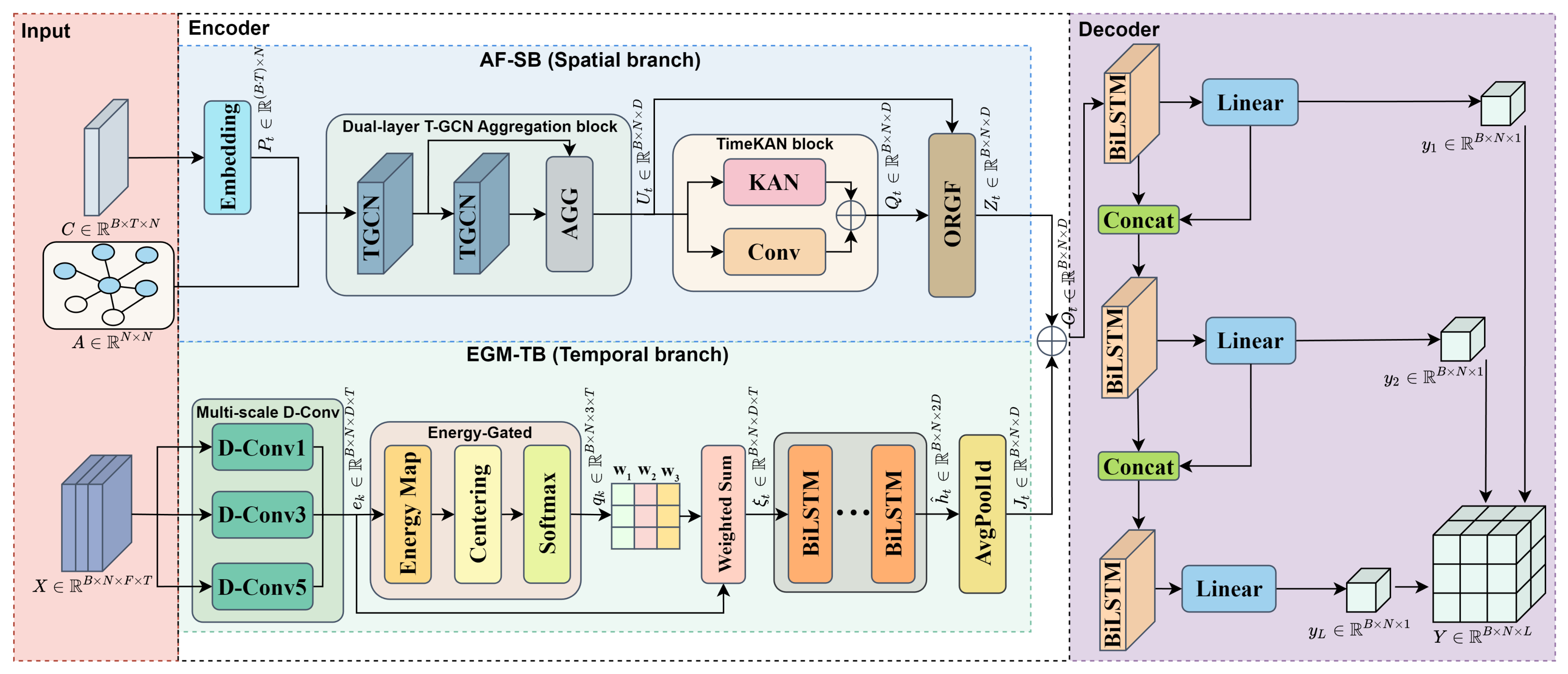
The overall architecture of STG-Mixer is shown in Figure 2. The model follows an encoder–decoder framework designed to jointly characterize interregional spatial associations and multi-timescale temporal patterns in HFMD surveillance data. The encoder consists of two parallel branches: the Adaptive Fusion Spatial Branch (AF-SB) and the Multi-Scale Energy-Gated Temporal Branch (MEG-TB). Their outputs are subsequently integrated to form a hybrid spatiotemporal representation, which is used by an autoregressive decoder to generate multi-step HFMD forecasts.

Figure 2. Overall architecture of the Spatiotemporal Graph Mixer (STG-Mixer).

The model takes the multivariate input sequence $\mathbf{X}$ and the regional adjacency matrix $\mathbf{A}$ as inputs. The multivariate sequence contains historical HFMD case counts, selected meteorological variables, and temporal sequence information, while $\mathbf{A}$ represents the geographical adjacency relationships among regions. Case-related features are extracted from $\mathbf{X}$ to form the case sequence ${\mathbf{C}}_t$, which is processed together with $\mathbf{A}$ by AF-SB to learn interregional spatial representations. In parallel, the complete multivariate sequence $\mathbf{X}$ is fed into MEG-TB to extract temporal representations at multiple timescales.

The spatial representation ${\mathbf{Z}}_t$ generated by AF-SB and the temporal representation ${\mathbf{J}}_t$ generated by MEG-TB are fused to obtain the hybrid spatiotemporal encoding ${\mathbf{O}}_t$. This representation is then passed to the autoregressive decoder, which progressively generates HFMD case-count forecasts for the subsequent L prediction steps across the target regions.

2.4.2. Adaptive Fusion Spatial Branch

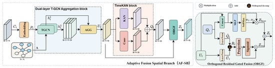
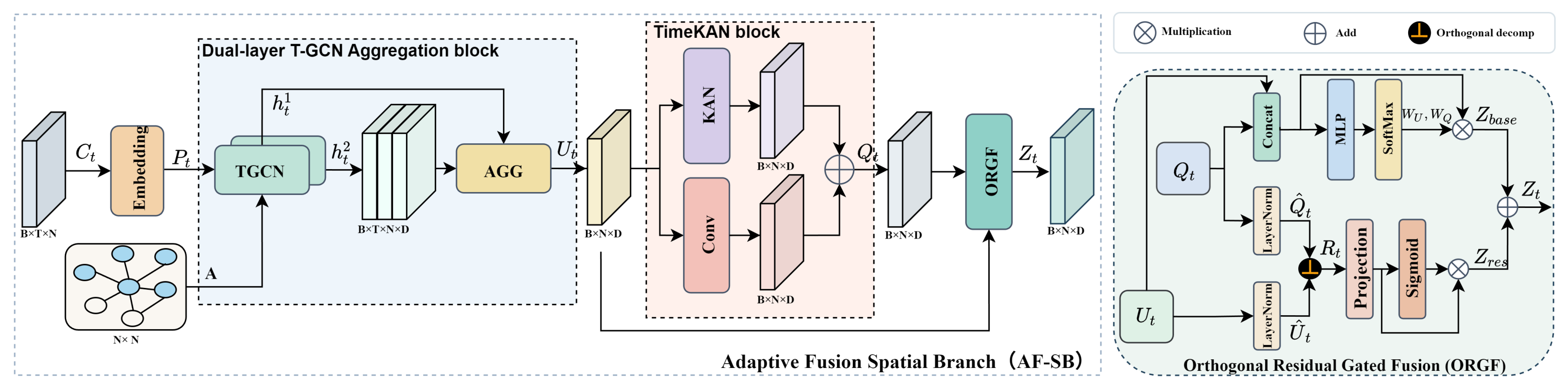
To capture spatial associations in multi-region HFMD surveillance data, we develop the Adaptive Fusion Spatial Branch (AF-SB), as shown in Figure 3. AF-SB learns interregional representations from historical HFMD case sequences and geographical adjacency information. It consists of an embedding block, a dual-layer T-GCN aggregation block, a TimeKAN block, and an Orthogonal Residual Gated Fusion (ORGF) module.

Figure 3. Overall structure of the Adaptive Fusion Spatial Branch (AF-SB).

The HFMD case sequence ${\mathbf{C}}_t$ is first transformed through a linear embedding followed by layer normalization to obtain the node representation ${\mathbf{P}}_t$. Guided by the adjacency matrix $\mathbf{A}$, two stacked T-GCN layers propagate and aggregate HFMD case information among geographically connected regions. The outputs of the two layers are combined using element-wise maximum aggregation, and the aggregated representation at the final time step is used as the spatial feature ${\mathbf{U}}_t$:

$$\begin{array}{cc}\hfill {\mathbf{h}}_t^1& ={\mathrm{TGCN}}_1({\mathbf{P}}_t,\mathbf{A}),\hfill \\ \hfill {\mathbf{h}}_t^2& ={\mathrm{TGCN}}_2({\mathbf{h}}_t^1,\mathbf{A}),\hfill \\ \hfill {\mathbf{U}}_t& =\max ({\mathbf{h}}_t^1,{\mathbf{h}}_t^2),\hfill \end{array}$$

(2)

where ${\mathbf{h}}_t^1$ and ${\mathbf{h}}_t^2$ denote the spatial representations generated by the two T-GCN layers, respectively, and ${\mathbf{U}}_t$ denotes the aggregated spatial feature.

To further characterize nonlinear relationships within the spatial representation, ${\mathbf{U}}_t$ is processed by the TimeKAN block. A Chebyshev polynomial transformation and a one-dimensional convolution are applied in parallel and subsequently fused:

$${\mathbf{Q}}_t={\mathcal{F}}_{\mathrm{cheby}}\left({\mathbf{U}}_t\right)+{\mathcal{F}}_{\mathrm{conv}}\left({\mathbf{U}}_t\right),$$

(3)

where ${\mathcal{F}}_{\mathrm{cheby}}(·)$ and ${\mathcal{F}}_{\mathrm{conv}}(·)$ denote the Chebyshev polynomial transformation and one-dimensional convolution operations, respectively.

The ORGF module is subsequently used to integrate ${\mathbf{U}}_t$ and ${\mathbf{Q}}_t$ through projection-based residual fusion. After layer normalization, the normalized representations are denoted by ${\widehat{\mathbf{U}}}_t$ and ${\widehat{\mathbf{Q}}}_t$. Two projection residuals are calculated by subtracting the projection of each representation onto the other, and their sum forms the residual representation:

$$\begin{array}{cc}\hfill {\mathbf{R}}_t=& \left({\widehat{\mathbf{Q}}}_t-{\displaystyle \frac{⟨{\widehat{\mathbf{Q}}}_t,{\widehat{\mathbf{U}}}_t⟩}{⟨{\widehat{\mathbf{U}}}_t,{\widehat{\mathbf{U}}}_t⟩}}{\widehat{\mathbf{U}}}_t\right)\hfill \\ \hfill & +\left({\widehat{\mathbf{U}}}_t-{\displaystyle \frac{⟨{\widehat{\mathbf{U}}}_t,{\widehat{\mathbf{Q}}}_t⟩}{⟨{\widehat{\mathbf{Q}}}_t,{\widehat{\mathbf{Q}}}_t⟩}}{\widehat{\mathbf{Q}}}_t\right),\hfill \end{array}$$

(4)

where $⟨·,·⟩$ denotes the inner product. The resulting residual representation is projected and filtered through a sigmoid gate:

$${\mathbf{Z}}_{\mathrm{res}}=\sigma \left(w_{\mathrm{res}}\mathrm{Pro}\left({\mathbf{R}}_t\right)+b_{\mathrm{res}}\right)\odot \mathrm{Pro}\left({\mathbf{R}}_t\right),$$

(5)

where $\mathrm{Pro}(·)$ denotes linear projection, $w_{\mathrm{res}}$ and $b_{\mathrm{res}}$ are learnable parameters, $\sigma (·)$ denotes the sigmoid activation function, and ⊙ denotes element-wise multiplication.

Meanwhile, ${\mathbf{U}}_t$ and ${\mathbf{Q}}_t$ are concatenated and passed through a multilayer perceptron (MLP) to estimate their adaptive fusion weights. The weighted base representation is then combined with the gated projection-based residual to obtain the final spatial representation:

$$\begin{array}{ccc}\hfill \left[{\mathbf{W}}_U,{\mathbf{W}}_Q\right]& =& \mathrm{Softmax}\left(\mathrm{MLP}\left[{\mathbf{U}}_t,{\mathbf{Q}}_t\right]\right),\hfill \\ \hfill {\mathbf{Z}}_{\mathrm{base}}& =& {\mathbf{W}}_U\odot {\mathbf{U}}_t+{\mathbf{W}}_Q\odot {\mathbf{Q}}_t,\hfill \\ \hfill {\mathbf{Z}}_t& =& {\mathbf{Z}}_{\mathrm{base}}+{\mathbf{Z}}_{\mathrm{res}}.\hfill \end{array}$$

(6)

Here, ${\mathbf{W}}_U$ and ${\mathbf{W}}_Q$ denote the adaptive weights assigned to the two spatial representations, and ${\mathbf{Z}}_t$ is the final output of AF-SB.

2.4.3. Multi-Scale Energy-Gated Temporal Branch

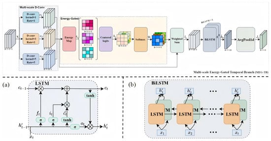
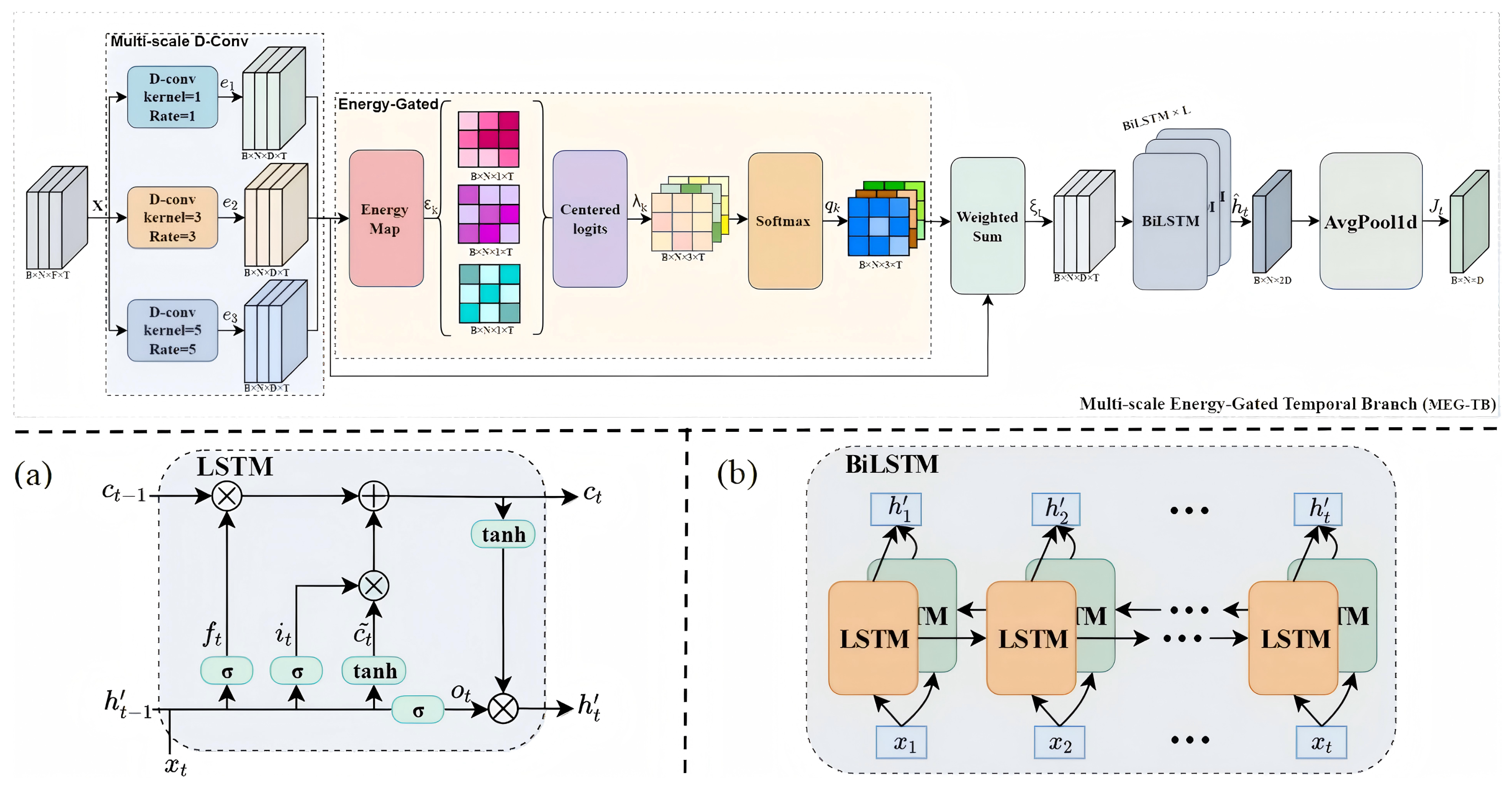
To characterize temporal dependencies between HFMD incidence and meteorological variables at different timescales, we develop the Multi-Scale Energy-Gated Temporal Branch (MEG-TB), as shown in Figure 4. MEG-TB consists of a multi-scale dilated convolution module, an energy-gated fusion module, a BiLSTM module, and an AvgPool1D layer. The multi-scale convolution module captures temporal patterns over different receptive fields, while the energy-gated mechanism adaptively emphasizes informative temporal-scale features before sequential dependency modeling.

Figure 4. Overall structure of the Multi-Scale Energy-Gated Temporal Branch (MEG-TB). (a) Structure of the LSTM unit. (b) BiLSTM architecture. BiLSTM × L denotes L BiLSTM layers corresponding to the L forecasting steps.

Given the multivariate input sequence $\mathbf{X}$, three parallel dilated temporal convolution branches are used to extract temporal features at different scales:

$${\mathbf{e}}_k={\mathrm{DConv}}_k\left(\mathbf{X}\right),k=1,2,3,$$

(7)

where ${\mathbf{e}}_k$ denotes the temporal representation extracted by the kth dilated convolution branch.

To estimate the relative importance of different temporal scales, an energy value is first calculated for each branch by averaging the squared feature responses across channels. The branch-wise energies are then centered and normalized using the Softmax function:

$$\begin{array}{ccc}\hfill {\epsilon }_k& =& {\displaystyle \frac{1}{C}}{\displaystyle \sum _{c=1}^C}{\left(e_{k,c}\right)}^2,\hfill \\ \hfill {\lambda }_k& =& {\epsilon }_k-\overline{\epsilon },\hfill \\ \hfill q_k& =& {\displaystyle \frac{\exp \left({\lambda }_k\right)}{{\sum }_{j=1}^3\exp \left({\lambda }_j\right)}},k=1,2,3,\hfill \end{array}$$

(8)

where C denotes the number of feature channels, $\overline{\epsilon }$ is the mean energy across the three branches, and $q_k$ denotes the adaptive weight assigned to the kth temporal scale.

The multi-timescale temporal features are then adaptively fused according to the energy-based weights:

$${\xi }_t={\displaystyle \sum _{k=1}^3}{q}_k{\mathbf{e}}_k,$$

(9)

where ${\xi }_t$ denotes the energy-weighted temporal representation.

The fused representation is subsequently processed by a BiLSTM to model sequential dependencies in both temporal directions. The resulting hidden representation is then reduced using one-dimensional average pooling to obtain the output of the temporal branch:

$$\begin{array}{ccc}\hfill {\widehat{\mathbf{h}}}_t& =& \mathrm{BiLSTM}\left({\xi }_t\right),\hfill \\ \hfill {\mathbf{J}}_t& =& \mathrm{AvgPool}1\mathrm{D}\left({\widehat{\mathbf{h}}}_t\right),\hfill \end{array}$$

(10)

where ${\widehat{\mathbf{h}}}_t$ denotes the bidirectional temporal representation and ${\mathbf{J}}_t$ is the final output of MEG-TB, which is subsequently fused with the spatial representation ${\mathbf{Z}}_t$.

2.4.4. Autoregressive Decoder

To generate multi-step HFMD forecasts from the hybrid spatiotemporal representation, STG-Mixer employs an autoregressive BiLSTM-based decoder. The decoder progressively produces future HFMD case counts, with the prediction from each forecasting step contributing to the input of the subsequent step.

The decoder receives the hybrid spatiotemporal representation $O_t\in {\mathbb{R}}^{B\times N\times D}$, where B denotes the batch size, N denotes the number of regional nodes, and D denotes the hidden feature dimension. The horizon-specific BiLSTM modules adopt a batch-first implementation; therefore, B remains the batch dimension and N serves as the internal sequence axis of each BiLSTM. No additional reshaping, flattening, or permutation is performed inside the decoder. Since the BiLSTM is bidirectional, its output has shape ${\mathbb{R}}^{B\times N\times 2D}$. Each forecasting horizon uses an independent BiLSTM module and an independent linear prediction head, and their parameters are not shared across forecasting horizons. The regional nodes follow a fixed node indexing that is maintained consistently throughout data preprocessing, graph construction, decoding, and evaluation, without additional node reordering inside the decoder.

At the first forecasting step, the hybrid spatiotemporal encoding ${\mathbf{O}}_t$ is processed by a BiLSTM layer, and the resulting hidden representation is mapped to the one-step-ahead HFMD prediction through a linear layer:

$$\begin{array}{ccc}\hfill {\mathbf{I}}_1& =& {\mathrm{BiLSTM}}_1\left({\mathbf{O}}_t\right),\hfill \\ \hfill {\widehat{\mathbf{y}}}_1& =& {\mathbf{W}}_1{\mathbf{I}}_1+{\mathbf{b}}_1,\hfill \end{array}$$

(11)

where ${\mathbf{I}}_1$ denotes the hidden representation at the first forecasting step, and ${\widehat{\mathbf{y}}}_1$ denotes the corresponding one-step-ahead HFMD case-count prediction. Accordingly, $I_1\in {\mathbb{R}}^{B\times N\times 2D}$ and ${\widehat{y}}_1\in {\mathbb{R}}^{B\times N\times 1}$. For $l\ge 2$, the previous hidden representation $I_{l-1}\in {\mathbb{R}}^{B\times N\times 2D}$ is concatenated with the previous prediction ${\widehat{y}}_{l-1}\in {\mathbb{R}}^{B\times N\times 1}$, forming an input tensor of ${\mathbb{R}}^{B\times N\times (2D+1)}$ for the next horizon-specific BiLSTM. The prediction-feedback mechanism is implemented identically during training and inference. Specifically, the model prediction generated at the preceding forecasting step is directly fed into the subsequent decoder stage. Ground-truth future HFMD observations are not used as decoder inputs during training; therefore, teacher forcing is not employed.

The recursive decoding process for the subsequent forecasting steps is expressed as

$$\begin{array}{ccc}\hfill {\mathbf{I}}_l& =& {\mathrm{BiLSTM}}_l\left(\mathrm{Concat}\left({\mathbf{I}}_{l-1},{\widehat{\mathbf{y}}}_{l-1}\right)\right),\hfill \\ \hfill {\widehat{\mathbf{y}}}_l& =& {\mathbf{W}}_l{\mathbf{I}}_l+{\mathbf{b}}_l,l=2,\dots ,L.\hfill \end{array}$$

(12)

The predictions from all forecasting steps are then concatenated to form the final multi-step forecasting output:

$$\widehat{\mathbf{Y}}=\mathrm{Concat}\left({\widehat{\mathbf{y}}}_1,{\widehat{\mathbf{y}}}_2,\dots ,{\widehat{\mathbf{y}}}_L\right),$$

(13)

where ${\mathbf{I}}_l$ and ${\widehat{\mathbf{y}}}_l$ denote the hidden representation and predicted HFMD case counts at the lth forecasting step, respectively. ${\mathbf{W}}_l$ and ${\mathbf{b}}_l$ are learnable parameters, and $\widehat{\mathbf{Y}}$ denotes the final multi-step forecasting output.

2.4.5. Loss Function

The model is trained by minimizing a squared-error objective over all regions and forecasting steps. An ${\mathit{\ell }}_2$ regularization term is additionally included to reduce overfitting:

$$\mathcal{L}={\displaystyle \frac{1}{2}}{\displaystyle \sum _{n=1}^N}{\displaystyle \sum _{l=1}^L}{\left(y_{n,l}-{\widehat{y}}_{n,l}\right)}^2+\lambda {\displaystyle \sum _{k=1}^K}{∥{\mathbf{w}}_k∥}_2^2,$$

(14)

where $y_{n,l}$ and ${\widehat{y}}_{n,l}$ denote the observed and predicted HFMD case counts for region n at forecasting step l, respectively. ${\mathbf{w}}_k$ denotes the kth learnable parameter, and $\lambda$ is the regularization coefficient.

2.5. Evaluation Protocol

STG-Mixer is evaluated under a multi-step forecasting setting with prediction horizons of $L\in \{1,2,3,4\}$. For the Japanese weekly dataset, these horizons correspond to one-, two-, three-, and four-week-ahead forecasting, respectively. For the Chinese daily dataset, they correspond to one-, two-, three-, and four-day-ahead forecasting.

Within each dataset, all models are evaluated using the same input variables, preprocessing procedures, chronological data partitions, and prediction horizons. For the Japanese dataset, model selection and hyperparameter adjustment are performed using the validation set, while the test set is reserved for final performance evaluation. The Chinese dataset is used as an independent external validation dataset to assess forecasting performance under a different temporal resolution. The hyperparameter configurations determined using the Japanese validation set were directly adopted for the Chinese experiments, and the Chinese test set was used exclusively for final performance evaluation. For the main comparative experiments, each model–forecasting-horizon configuration was evaluated once under the corresponding experimental setting. No additional evaluation mask was applied when calculating RMSE, MAE, or $R^2$, because missing observations had already been handled during data preprocessing. For each forecasting task with horizon L, all forecasting steps in the L-step output were included in the evaluation rather than only the final forecasting step. Within each evaluation batch, the forecasting-step dimension was incorporated into the sample dimension. Both predictions and observations were then transformed back to the original HFMD case-count scale using the Min–Max parameters corresponding to the HFMD case-count variable, with the same inverse-normalization parameters applied to both. RMSE, MAE, and $R^2$ were calculated across all corresponding predictions and target regions within each batch, and the resulting batch-level metrics were subsequently aggregated over the evaluation epoch to obtain the reported performance values.

2.6. Baseline Models

STG-Mixer is compared with representative forecasting models from different methodological categories, including the statistical model ARIMA, the machine learning model XGBoost, recurrent sequence models DA-RNN [36], Seq2Seq-Shih [22], and LSTM, transformer-based models ST-Transformer [37] and ORIT [38], and graph-based spatiotemporal models T-GCN and STGCN [39].

ARIMA is a conventional statistical time-series forecasting model, whereas XGBoost is a tree-based ensemble learning method. DA-RNN, Seq2Seq-Shih, and LSTM represent recurrent sequence forecasting approaches. Seq2Seq-Shih is a sequence-to-sequence forecasting model incorporating the Shih attention mechanism, which introduces an attention module to capture informative temporal patterns from historical observations for multi-step forecasting. ST-Transformer and ORIT represent attention- or transformer-based forecasting models. T-GCN and STGCN are graph-based spatiotemporal models that explicitly incorporate regional relationships.

All baseline models are trained and evaluated under the same experimental protocol as STG-Mixer within each dataset. The same chronological data partitions and prediction horizons are used for all comparative experiments, and model configurations follow the corresponding implementations adopted in this study.

For the deep learning baseline models, architecture-specific configurations followed their corresponding implementations, while model selection on the Japanese dataset followed the same validation-based principle used for STG-Mixer. The test set was not used for hyperparameter selection. Because the compared models have different architectures and parameterizations, identical numerical hyperparameter ranges were not imposed; instead, the same data partitions and forecasting horizons were used to ensure a fair comparison. For the Chinese dataset, the configurations determined on the Japanese dataset were directly adopted.

2.7. Evaluation Metrics

Forecasting performance is evaluated using the root mean square error (RMSE), mean absolute error (MAE), and coefficient of determination ($R^2$). Each metric is calculated separately for each prediction horizon across all test samples and regions.

RMSE is defined as

$$\mathrm{RMSE}=\sqrt{{\displaystyle \frac{1}{MN}}\sum _{m=1}^M\sum _{i=1}^N{\left(y_{m,i}-{\widehat{y}}_{m,i}\right)}^2},$$

(15)

MAE is defined as

$$\mathrm{MAE}={\displaystyle \frac{1}{MN}}{\displaystyle \sum _{m=1}^M}{\displaystyle \sum _{i=1}^N}\left|y_{m,i}-{\widehat{y}}_{m,i}\right|,$$

(16)

and $R^2$ is defined as

$$R^2=1-{\displaystyle \frac{{\displaystyle {\displaystyle \sum _{m=1}^M}{\displaystyle \sum _{i=1}^N}{\left(y_{m,i}-{\widehat{y}}_{m,i}\right)}^2}}{{\displaystyle {\displaystyle \sum _{m=1}^M}{\displaystyle \sum _{i=1}^N}{\left(y_{m,i}-\overline{y}\right)}^2}}},$$

(17)

where $y_{m,i}$ and ${\widehat{y}}_{m,i}$ denote the observed and predicted HFMD case counts for region i in test sample m, respectively. M and N denote the numbers of test samples and regions, respectively, and $\overline{y}$ denotes the mean of the observed values. Lower RMSE and MAE values indicate smaller forecasting errors, whereas higher $R^2$ values indicate better forecasting performance.

2.8. Implementation Details

All experiments were conducted on a workstation running Ubuntu 24.04.3 LTS with 64 GB of RAM and four NVIDIA GeForce RTX 3060 GPUs, each with 12 GB of GPU memory. The deep learning models were implemented in Python 3.7.12 using PyTorch 1.12.0 with CUDA 11.6.

The maximum number of training epochs was set to 500 for all deep learning models. All deep learning models were optimized using the Adam optimizer. For STG-Mixer, the dilation rates of the three temporal convolution branches were set to (1, 3, 5), as illustrated in Figure 4. The L2 regularization coefficient was set to 0.003. Early stopping was performed based on the validation $R^2$, with a patience of 50 epochs and a minimum improvement threshold of 0.001. For the Japanese dataset, hyperparameters were selected according to the validation performance, while the test set was reserved exclusively for final evaluation. The historical input-window length was selected separately for each forecasting horizon. Once selected, the remaining model and optimization settings were fixed during the corresponding comparative experiments.

The main hyperparameter settings and implementation details of STG-Mixer and the baseline models are summarized in Table 2. These configurations were subsequently adopted for the Chinese dataset. For the traditional machine learning and statistical baselines, XGBoost was configured with 1000 boosting estimators, a maximum tree depth of 6, a learning rate of 0.03, a subsampling ratio of 0.8, and a column-sampling ratio of 0.8. The L1 and L2 regularization coefficients were set to 0 and 1, respectively. ARIMA was implemented with a fixed order of (1, 1, 1), without automatic order selection. These configurations were kept fixed across the evaluated forecasting horizons and datasets.

Table 2. Main hyperparameter settings and implementation details of STG-Mixer and baseline models.

Model	Input Length (T)	Batch Size	Hidden Dimension	Learning Rate	Weight Decay	Optimizer
STG-Mixer	3/3/4/6	16	128	0.001	0.0015	Adam
DA-RNN	3/3/4/4	16	128	0.001	0.0015	Adam
ST-Transformer	3/3/4/6	16	128	0.001	0.0015	Adam
T-GCN	3/3/4/6	16	128	0.002	0.0015	Adam
Seq2Seq-Shih	3/3/4/6	16	128	0.002	0.0015	Adam
LSTM	3/3/4/6	16	256	0.001	0.0015	Adam
STGCN	3/3/4/4	16	128	0.001	0.0015	Adam
ORIT	3/3/4/4	32	128	0.002	0.0015	Adam

3. Results

3.1. Forecasting Performance on the Japanese Dataset

As shown in Table 3, forecasting performance generally decreased as the prediction horizon increased from $L=1$ to $L=4$, with higher MAE and RMSE values and lower $R^2$ values observed at longer horizons. STG-Mixer consistently achieved the best overall performance among the compared models across all four forecasting horizons. In particular, it achieved $R^2$ values of 0.965, 0.908, 0.834, and 0.787 for one-, two-, three-, and four-week-ahead forecasting, respectively, while also obtaining the lowest MAE and RMSE at each horizon. Although forecasting performance declined with increasing prediction horizon, STG-Mixer maintained a clear advantage over the baseline models, including at the longer three- and four-week-ahead horizons. These results demonstrate the effectiveness of STG-Mixer for multi-region HFMD forecasting on the Japanese dataset.

Table 3. Comparison results under different prediction horizons on the Japanese multi-region HFMD dataset. For this weekly dataset, $L=1,2,3,4$ correspond to one- to four-week-ahead forecasting, respectively.

Model	$\mathit{L}=1$			$\mathit{L}=2$			$\mathit{L}=3$			$\mathit{L}=4$
	${\mathbf{R}}^{\mathbf{2}}$	MAE	RMSE	${\mathbf{R}}^{\mathbf{2}}$	MAE	RMSE	${\mathbf{R}}^{\mathbf{2}}$	MAE	RMSE	${\mathbf{R}}^{\mathbf{2}}$	MAE	RMSE
STG-Mixer	0.965	12.32	21.40	0.908	17.69	34.85	0.834	24.91	47.01	0.787	25.29	52.51
DA-RNN	0.915	15.94	33.45	0.848	22.31	45.01	0.779	27.58	54.50	0.713	28.41	62.48
Seq2Seq-Shih	0.916	14.51	33.34	0.835	24.50	46.77	0.772	28.28	55.03	0.687	33.46	64.45
LSTM	0.927	14.29	31.03	0.857	22.09	43.40	0.782	28.15	53.82	0.728	28.91	60.07
T-GCN	0.578	37.93	74.91	0.547	38.61	77.41	0.523	39.81	80.23	0.485	43.84	82.54
XGBoost	0.895	21.06	37.25	0.795	25.19	52.35	0.700	28.80	63.37	0.670	33.11	65.85
STGCN	0.787	29.04	53.02	0.626	39.49	71.03	0.569	39.51	76.83	0.528	40.31	78.30
ORIT	0.910	14.65	34.14	0.838	20.03	46.01	0.798	24.98	52.28	0.714	30.47	61.79
ARIMA	0.921	14.18	32.15	0.854	18.01	44.15	0.789	25.18	52.49	0.704	28.60	63.35
ST-Transformer	0.858	25.05	43.44	0.824	25.53	48.60	0.751	29.57	57.93	0.689	33.34	64.00

3.2. Forecasting Performance on the Independent Chinese Dataset

To further evaluate STG-Mixer using an independent dataset with a different temporal resolution, additional experiments were conducted using the HFMD dataset from southern China. For this daily dataset, the prediction horizons $L=1,2,3,4$ correspond to one-, two-, three-, and four-day-ahead forecasting, respectively. As shown in Table 4, STG-Mixer achieved the best overall performance across all four forecasting horizons. Specifically, the model obtained $R^2$ values of 0.888, 0.875, 0.834, and 0.829 for $L=1$ to $L=4$, respectively, while also achieving the lowest MAE and RMSE at each horizon. Although forecasting performance decreased slightly as the prediction horizon increased, STG-Mixer maintained a consistent advantage over the compared models. These results indicate that the proposed framework retains effective forecasting performance under a different temporal resolution and an independent surveillance setting.

Table 4. Comparison results under different prediction horizons on the HFMD dataset from a city in southern China. For this daily dataset, $L=1,2,3,4$ correspond to one- to four-day-ahead forecasting, respectively.

Model	$\mathit{L}=1$			$\mathit{L}=2$			$\mathit{L}=3$			$\mathit{L}=4$
	${\mathbf{R}}^{\mathbf{2}}$	MAE	RMSE	${\mathbf{R}}^{\mathbf{2}}$	MAE	RMSE	${\mathbf{R}}^{\mathbf{2}}$	MAE	RMSE	${\mathbf{R}}^{\mathbf{2}}$	MAE	RMSE
STG-Mixer	0.888	8.15	10.84	0.875	8.63	11.54	0.834	9.88	13.33	0.829	10.02	13.52
DA-RNN	0.761	12.97	16.03	0.651	16.01	19.37	0.615	16.81	20.37	0.551	18.49	22.01
Seq2Seq-Shih	0.832	9.87	13.41	0.820	10.02	13.68	0.800	10.67	14.52	0.788	11.67	15.00
LSTM	0.852	9.07	12.51	0.823	9.86	13.68	0.798	11.08	14.64	0.786	11.21	15.03
T-GCN	0.816	10.23	13.90	0.789	10.99	14.89	0.781	11.25	15.25	0.750	12.64	16.26
XGBoost	0.808	10.49	14.22	0.763	11.58	15.83	0.776	11.18	15.36	0.730	12.42	16.88
STGCN	0.840	9.71	12.95	0.800	10.99	14.49	0.789	10.81	14.89	0.564	17.07	21.39
ORIT	0.787	11.46	15.14	0.771	11.79	15.70	0.766	12.03	15.88	0.750	12.48	16.42
ARIMA	0.849	9.12	12.60	0.816	10.04	13.91	0.792	10.67	14.80	0.776	11.06	15.37
ST-Transformer	0.835	9.93	13.34	0.797	10.99	14.90	0.733	13.11	17.09	0.726	13.35	17.27

3.3. Regional and Multi-Step Forecasting Performance

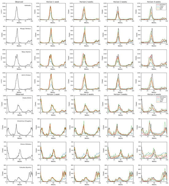
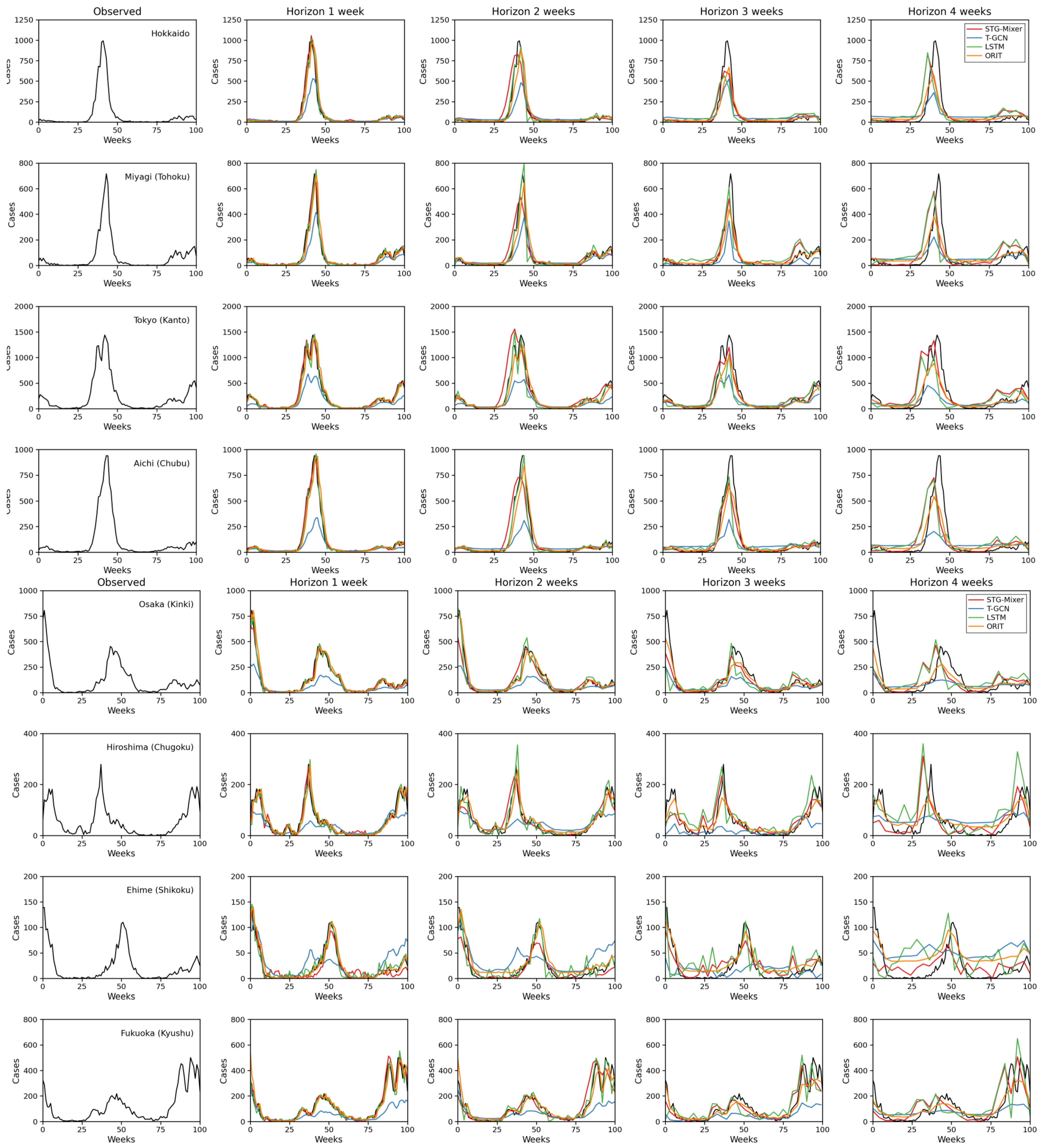
To further examine forecasting performance across different regions and prediction horizons, one representative prefecture was selected from each of Japan’s eight regions. The observed HFMD cases and one- to four-week-ahead forecasts are shown in Figure 5. For the one- and two-week-ahead tasks, most models captured the major temporal patterns and epidemic peaks to some extent. As the prediction horizon increased to three and four weeks, larger deviations in peak timing and magnitude were observed for several baseline models. In contrast, STG-Mixer generally maintained closer agreement with the observed HFMD trajectories across the representative prefectures. For example, in Osaka and Hiroshima, STG-Mixer more closely reproduced the overall temporal trends and peak magnitudes across most forecasting horizons, although some peak displacement remained in the four-week-ahead forecasts. These results indicate that STG-Mixer maintains comparatively consistent regional forecasting performance as the prediction horizon increases.

Figure 5. Comparison of observed HFMD cases and one- to four-week-ahead forecasting results for eight representative prefectures in Japan: Hokkaido, Miyagi, Tokyo, Aichi, Osaka, Hiroshima, Ehime, and Fukuoka.

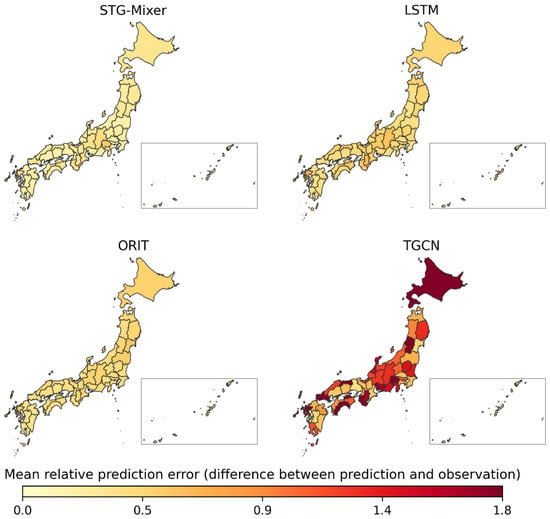
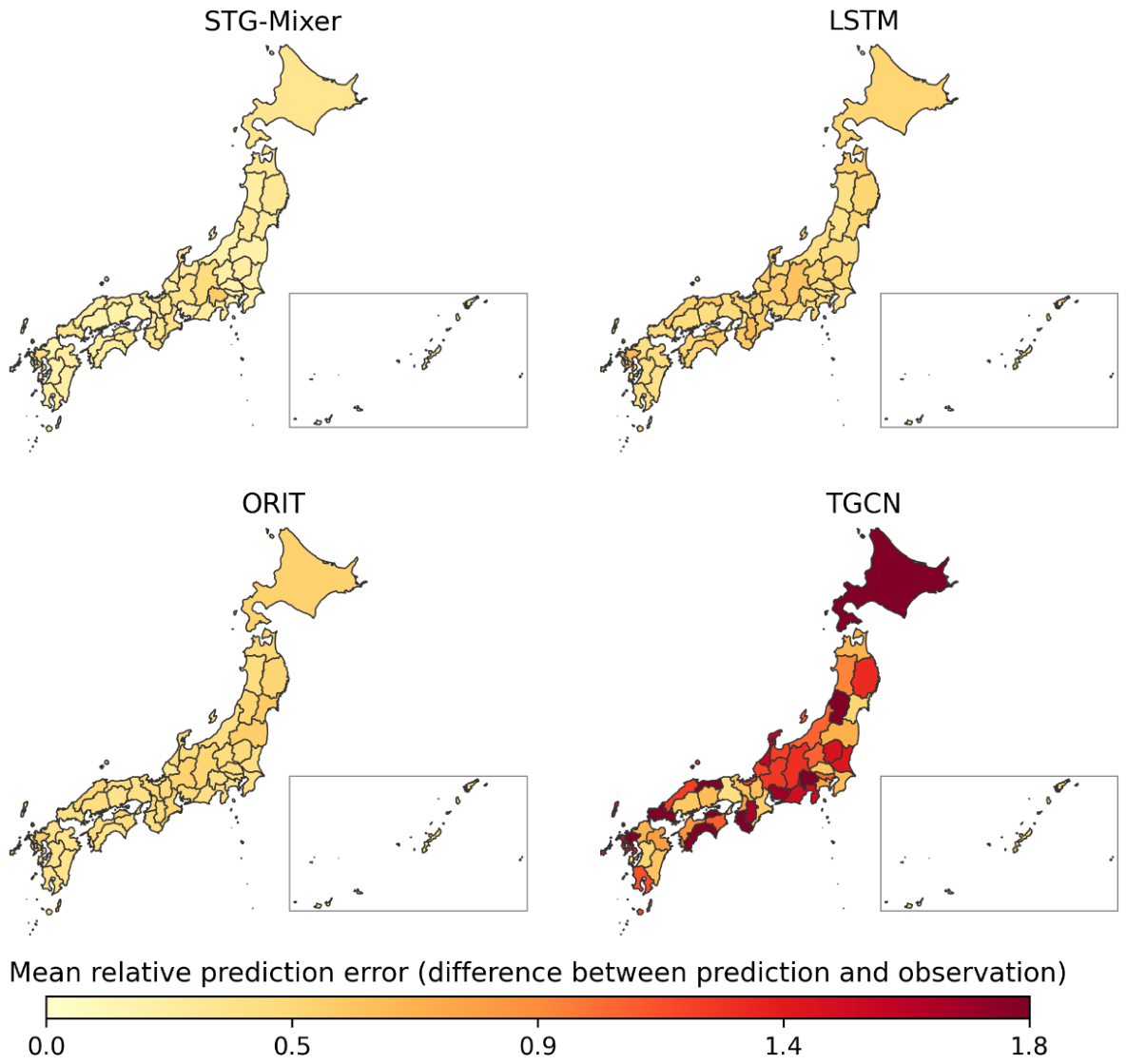
Figure 6 further shows the spatial distribution of the mean relative prediction error across Japan’s 47 prefectures for one-week-ahead forecasting. STG-Mixer exhibited relatively low prediction errors across most prefectures, including representative regions such as Hokkaido and Tokyo, whereas T-GCN showed substantially larger errors in several eastern regions. The spatial error distribution indicates that the forecasting performance of STG-Mixer was not restricted to a small number of well-predicted prefectures, but remained comparatively consistent across the Japanese multi-region dataset.

Figure 6. Spatial distribution of mean relative prediction error for one-week-ahead HFMD forecasting across Japan.

3.4. Model Component Analysis

To assess the contribution of the main components of STG-Mixer, we conducted model component analysis on the Japanese multi-region HFMD dataset. Five reduced variants were evaluated by removing the ORGF module (w/o O), the TimeKAN block (w/o TimeKAN), the energy-gated module (w/o EG), the multi-scale temporal modeling module (w/o Multi), and the BiLSTM module in MEG-TB (w/o BiLSTM), respectively. All variants were trained and evaluated under the same experimental settings as the complete model. The results for one- to four-week-ahead forecasting are summarized in Table 5.

Table 5. Model component analysis results of STG-Mixer on the Japanese multi-region HFMD dataset, where $L=1,2,3,4$ denote one- to four-week-ahead forecasting tasks, respectively.

Model	$\mathit{L}=1$			$\mathit{L}=2$			$\mathit{L}=3$			$\mathit{L}=4$
	${\mathbf{R}}^{\mathbf{2}}$	MAE	RMSE	${\mathbf{R}}^{\mathbf{2}}$	MAE	RMSE	${\mathbf{R}}^{\mathbf{2}}$	MAE	RMSE	${\mathbf{R}}^{\mathbf{2}}$	MAE	RMSE
STG-Mixer	0.965	12.32	21.40	0.908	17.69	34.85	0.834	24.91	47.01	0.787	25.29	52.51
w/o O	0.960	13.78	22.81	0.900	19.18	36.27	0.829	25.70	48.20	0.768	27.90	56.50
w/o TimeKAN	0.957	13.80	23.60	0.882	20.30	39.80	0.822	26.10	49.10	0.755	28.70	58.20
w/o EG	0.952	14.60	25.10	0.875	21.10	41.10	0.816	26.41	49.71	0.743	29.40	59.60
w/o Multi	0.945	15.20	26.80	0.869	21.60	42.00	0.808	26.62	50.59	0.731	29.80	60.80
w/o BiLSTM	0.926	15.93	30.94	0.858	23.23	43.21	0.805	27.30	51.00	0.715	30.33	61.18

Across all forecasting horizons, the complete STG-Mixer consistently outperformed the reduced variants, indicating that the evaluated components contribute complementarily to forecasting performance. In the four-week-ahead task, the complete model achieved an $R^2$ of 0.787 and an RMSE of 52.51, whereas the reduced variants obtained $R^2$ values ranging from 0.715 to 0.768 and RMSE values ranging from 56.50 to 61.18.

Removing ORGF (w/o O) resulted in a consistent performance decline. At $L=4$, $R^2$ decreased from 0.787 to 0.768 and RMSE increased from 52.51 to 56.50, indicating that the inclusion of ORGF contributes to improved forecasting performance.

Removing the TimeKAN block produced a larger performance reduction at longer forecasting horizons. In the four-week-ahead task, the w/o TimeKAN variant achieved an $R^2$ of 0.755 and an RMSE of 58.20, suggesting that nonlinear transformation of the spatial representation contributes to multi-step forecasting performance.

The removal of the energy-gated module (w/o EG) also reduced forecasting accuracy across the evaluated horizons. For example, at $L=2$, $R^2$ decreased from 0.908 to 0.875, supporting the contribution of adaptive weighting among temporal-scale features.

The w/o Multi variant, which removes the multi-scale temporal modeling module, showed a pronounced performance decrease at longer horizons. At $L=4$, its $R^2$ decreased to 0.731 and its RMSE increased to 60.80, indicating the importance of extracting temporal information at multiple scales.

Among the reduced variants, removing the BiLSTM module in MEG-TB produced the largest overall performance degradation. The w/o BiLSTM variant achieved an $R^2$ of 0.715 and an RMSE of 61.18 at $L=4$, showing that sequential dependency modeling is an important component of the temporal branch for multi-step HFMD forecasting.

3.5. Sensitivity to Spatial Graph Structure

To further examine the influence of spatial graph construction on forecasting performance, we conducted two additional comparisons while keeping all other model components and experimental settings unchanged. First, a dynamic indicator-based weighted graph was constructed from region-specific HFMD incidence, temperature, precipitation, and relative humidity. These indicators were standardized across regions, and the pairwise similarity between regional indicator vectors was converted into dynamic edge weights using a Gaussian radial basis function. Consequently, the spatial connections varied according to the epidemiological and meteorological states of the regions. Importantly, the dynamic graph was constructed using only historical HFMD incidence and meteorological observations available before each forecasting origin, without incorporating any observations from the prediction period, thereby preventing future information leakage. Second, to isolate the contribution of interregional message passing, the original geographical adjacency matrix was replaced with an identity adjacency matrix. Under this setting, only self-connections were retained and all edges between different prefectures were removed, thereby disabling interregional message passing through the graph convolutional layers. The results are summarized in Table 6.

Table 6. Sensitivity analysis of different spatial graph structures on the Japanese multi-region HFMD dataset, where $L=1,2,3,4$ denote one- to four-week-ahead forecasting tasks, respectively.

Spatial Graph	$\mathit{L}=1$			$\mathit{L}=2$			$\mathit{L}=3$			$\mathit{L}=4$
	${\mathbf{R}}^{\mathbf{2}}$	MAE	RMSE	${\mathbf{R}}^{\mathbf{2}}$	MAE	RMSE	${\mathbf{R}}^{\mathbf{2}}$	MAE	RMSE	${\mathbf{R}}^{\mathbf{2}}$	MAE	RMSE
Adjacency-based	0.965	12.32	21.40	0.908	17.69	34.85	0.834	24.91	47.01	0.787	25.29	52.51
Dynamic indicator-based	0.960	12.35	22.89	0.893	20.54	37.60	0.795	25.06	53.01	0.738	27.75	59.24
Identity adjacency	0.943	15.36	27.25	0.866	22.20	42.83	0.769	27.32	54.90	0.714	36.71	62.89

As shown in Table 6, the original geographical adjacency graph achieved better forecasting performance than the dynamic indicator-based graph across all four forecasting horizons. At $L=1$, the difference was relatively small, with $R^2$ values of 0.965 and 0.960 for the adjacency-based and dynamic graphs, respectively. As the forecasting horizon increased, the differences in $R^2$ and RMSE generally became more evident. At $L=4$, the adjacency-based graph achieved an $R^2$ of 0.787, an MAE of 25.29, and an RMSE of 52.51, whereas the dynamic indicator-based graph obtained an $R^2$ of 0.738, an MAE of 27.75, and an RMSE of 59.24. These results indicate that, although the dynamic graph can adaptively capture short-term similarities in regional epidemiological and meteorological conditions, the fixed geographical adjacency structure yields better forecasting performance on this dataset.

Compared with the identity-adjacency variant, the original geographical graph also achieved consistently higher $R^2$ and lower MAE and RMSE across all four horizons. In particular, at $L=4$, replacing geographical adjacency with the identity matrix decreased $R^2$ from 0.787 to 0.714 and increased MAE and RMSE from 25.29 and 52.51 to 36.71 and 62.89, respectively. Since this comparison removes edges between distinct prefectures while retaining the remaining model structure, the observed degradation supports the contribution of graph-based interregional message passing to forecasting accuracy.

3.6. Comparison of Decoding Strategies

To evaluate the effect of the decoding strategy, we further compared the proposed autoregressive decoder with a direct multi-horizon decoder. In the direct setting, the same encoded spatiotemporal representation was used to predict all future horizons simultaneously without feeding previous predictions into subsequent decoding steps, while all other model components and experimental settings were kept unchanged. The results are summarized in Table 7.

Table 7. Comparison of autoregressive and direct multi-horizon decoding strategies on the Japanese multi-region HFMD dataset, where $L=1,2,3,4$ denote one- to four-week-ahead forecasting tasks, respectively.

Decoding Strategy	$\mathit{L}=1$			$\mathit{L}=2$			$\mathit{L}=3$			$\mathit{L}=4$
	${\mathbf{R}}^{\mathbf{2}}$	MAE	RMSE	${\mathbf{R}}^{\mathbf{2}}$	MAE	RMSE	${\mathbf{R}}^{\mathbf{2}}$	MAE	RMSE	${\mathbf{R}}^{\mathbf{2}}$	MAE	RMSE
Autoregressive	0.965	12.32	21.40	0.908	17.69	34.85	0.834	24.91	47.01	0.787	25.29	52.51
Direct multi-horizon	0.914	17.05	33.68	0.882	20.14	39.58	0.797	25.53	52.38	0.731	27.10	61.89

Overall, the autoregressive decoder achieved better forecasting performance across all evaluated horizons. It consistently obtained higher $R^2$ values and lower MAE and RMSE values than the direct multi-horizon decoder for $L=1$–4. At $L=4$, the autoregressive decoder achieved an $R^2$ of 0.787, an MAE of 25.29, and an RMSE of 52.51, whereas the direct multi-horizon decoder obtained an $R^2$ of 0.731, an MAE of 27.10, and an RMSE of 61.89. These results suggest that explicitly propagating information across successive forecasting steps is beneficial for multi-step HFMD forecasting in this dataset, despite the potential risk of recursive error accumulation.

3.7. Sensitivity to Historical Input Length

To further examine the influence of historical input-window length on forecasting performance, we conducted a sensitivity analysis on the Japanese multi-region HFMD dataset across all four forecasting horizons. For each forecasting task with $L\in \{1,2,3,4\}$, the historical input length T was varied among 3, 4, 5, and 6, while the remaining model architecture and training settings were kept unchanged. The results are summarized in Table 8.

Table 8. Sensitivity analysis of historical input length across one- to four-week-ahead forecasting tasks on the Japanese multi-region HFMD dataset.

Prediction Horizon	Input Length T	${\mathit{R}}^2$	MAE	RMSE
$L=1$	3	0.965	12.32	21.40
	4	0.960	12.34	22.77
	5	0.958	13.74	23.47
	6	0.954	13.98	24.45
$L=2$	3	0.908	17.69	34.85
	4	0.906	18.35	35.23
	5	0.896	19.23	37.04
	6	0.890	21.05	38.19
$L=3$	3	0.814	25.29	50.00
	4	0.834	24.91	47.01
	5	0.808	25.34	50.58
	6	0.774	26.12	55.02
$L=4$	3	0.748	30.91	57.76
	4	0.755	28.60	56.39
	5	0.777	25.88	53.85
	6	0.787	25.29	52.51

As shown in Table 8, the influence of historical input length varied across different forecasting horizons. For one- and two-week-ahead forecasting, the best performance was obtained at $T=3$, and increasing the input length led to a gradual decline in forecasting accuracy. For three-week-ahead forecasting, $T=4$ achieved the best results, with an $R^2$ of 0.834, an MAE of 24.91, and an RMSE of 47.01, while both shorter and longer input windows resulted in reduced performance. In contrast, for four-week-ahead forecasting, performance improved as the input length increased from $T=3$ to $T=6$, with the best results achieved at $T=6$, yielding an $R^2$ of 0.787, an MAE of 25.29, and an RMSE of 52.51. These findings indicate that the appropriate historical input length varies across forecasting horizons. Within the evaluated range, shorter input windows were more effective for short-term forecasting, whereas a longer historical window was beneficial for the four-week-ahead task. The results also support the input-length configurations of $T=3$, $T=3$, $T=4$, and $T=6$ adopted in the main experiments.

3.8. Robustness and Reproducibility Analysis

To further assess the robustness of STG-Mixer to random initialization, we repeated the experiments using five different random seeds, namely 41, 42, 45, 46, and 48. The seed 42 corresponds to the setting used for the main experimental results. All other model configurations, data partitions, and training settings were kept unchanged across runs. The mean and standard deviation of $R^2$, MAE, and RMSE across the five independent runs are reported in Table 9.

Table 9. Robustness analysis of STG-Mixer using five random seeds on the Japanese multi-region HFMD dataset. For this weekly dataset, $L=1,2,3,4$ correspond to one- to four-week-ahead forecasting, respectively.

Prediction Horizon	${\mathit{R}}^2$	MAE	RMSE
$L=1$	$0.958\pm 0.008$	$12.52\pm 0.84$	$23.35\pm 2.22$
$L=2$	$0.917\pm 0.012$	$16.79\pm 0.94$	$33.11\pm 2.50$
$L=3$	$0.845\pm 0.011$	$23.58\pm 1.46$	$45.43\pm 1.69$
$L=4$	$0.781\pm 0.022$	$25.92\pm 1.14$	$53.41\pm 2.88$

As shown in Table 9, STG-Mixer maintained consistent forecasting performance across different random seeds. The standard deviations remained relatively small across all four forecasting horizons, indicating that the performance of the proposed model is not strongly dependent on a particular random initialization. Although the variability increased slightly for the longer forecasting horizon, the overall results demonstrate stable predictive performance across independent runs.

To further examine the reproducibility of STG-Mixer under identical experimental conditions, each forecasting experiment was independently repeated five times using the same training command, random seed, data partition, model configuration, and hyperparameter settings. The mean and standard deviation of $R^2$, MAE, and RMSE across the five repeated runs are reported in Table 10.

Table 10. Reproducibility analysis of STG-Mixer under identical experimental settings on the Japanese multi-region HFMD dataset.

Prediction Horizon	${\mathit{R}}^2$	MAE	RMSE
$L=1$	$0.9645\pm 0.0005$	$12.07\pm 0.49$	$21.58\pm 0.19$
$L=2$	$0.9093\pm 0.0009$	$17.50\pm 0.19$	$34.65\pm 0.21$
$L=3$	$0.8330\pm 0.0026$	$24.92\pm 0.02$	$47.10\pm 0.16$
$L=4$	$0.7884\pm 0.0008$	$26.06\pm 0.78$	$52.47\pm 0.04$

As shown in Table 10, only minor variations were observed across repeated runs under identical experimental settings. The standard deviations of $R^2$ and RMSE remained small across all four forecasting horizons, indicating that STG-Mixer exhibits stable and reproducible forecasting performance when the same experimental configuration is used. The repeated experiments were performed with GPU acceleration. Despite the fixed random seed and identical training settings, these minor variations may arise from numerical nondeterminism associated with parallel floating-point computations on GPU/CUDA.

4. Discussion

The forecasting performance of all models generally decreased as the prediction horizon increased, reflecting the greater difficulty of maintaining accurate forecasts over longer horizons. Sequence-based models such as LSTM and DA-RNN showed competitive performance at shorter horizons but exhibited greater performance degradation as the forecasting horizon increased. This pattern suggests that temporal dependency modeling alone may be insufficient when multi-step HFMD forecasting requires the simultaneous representation of temporal dynamics and interregional associations. In comparison, STG-Mixer maintained a more consistent advantage across different forecasting horizons by jointly modeling multi-timescale temporal patterns and spatial associations. From a disease surveillance perspective, maintaining reliable performance at longer forecasting horizons may provide additional lead time for epidemic trend assessment, preparedness, and resource planning.

Graph-based models explicitly incorporate spatial relationships among regions, but their forecasting performance depends on how spatial information is represented and integrated with temporal dynamics. In this study, T-GCN and STGCN showed weaker performance than STG-Mixer, particularly at longer forecasting horizons. One possible reason is that directly combining graph-based spatial aggregation with conventional temporal modeling may not be sufficient to capture the heterogeneous and nonlinear relationships present in multi-region HFMD surveillance data. STG-Mixer addresses this limitation through its Adaptive Fusion Spatial Branch, which combines graph-based aggregation, nonlinear transformation, and orthogonal residual gated fusion before integrating the resulting spatial representation with multi-timescale temporal features. The improved performance observed across forecasting horizons therefore supports the usefulness of jointly refining spatial representations and temporal dependencies rather than modeling them in a more loosely coupled manner.

The model component analysis provides further insight into how the different modules contribute to the overall forecasting framework. The performance declines observed after removing ORGF and TimeKAN indicate that both components contribute to improved forecasting performance. Similarly, the reductions associated with removing the energy-gated and multi-scale temporal modules indicate that temporal information at different scales should not be treated equally or modeled at a single temporal resolution. The largest degradation occurred when the BiLSTM module in MEG-TB was removed, highlighting the importance of sequential dependency modeling after multi-scale temporal feature extraction. Taken together, these findings suggest that the performance of STG-Mixer is not attributable to a single module, but rather to the complementary interaction between spatial representation learning, multi-timescale temporal modeling, adaptive feature weighting, and sequential dependency modeling.

The evaluation on the independent HFMD dataset from a city in southern China provides additional external validation of the forecasting capability of STG-Mixer under a different temporal resolution. Unlike the Japanese dataset, which contains weekly observations from 47 prefectures, the Chinese dataset consists of daily observations from a single city. Despite the difference in temporal resolution and surveillance setting, STG-Mixer maintained competitive forecasting performance across the evaluated horizons. This result suggests that the proposed framework can retain effective forecasting performance when applied to an independent HFMD surveillance dataset with different temporal characteristics. Nevertheless, broader validation across additional regions and surveillance systems will be necessary to further assess its generalizability.

This study has several limitations. First, the model relies on historical meteorological observations as exogenous inputs but does not explicitly account for the uncertainty associated with these external factors. Changes in meteorological conditions beyond the observed input window may therefore introduce additional uncertainty into multi-step HFMD forecasting. Second, although a dynamic indicator-based graph was additionally evaluated, the adopted graph structures may still not fully capture complex epidemiological connections such as population mobility and transportation links. Third, although this study incorporates HFMD case counts, meteorological variables, and temporal sequence features, it does not explicitly include broader social, economic, behavioral, demographic, or policy-related factors that may influence HFMD incidence. Such factors are difficult to comprehensively quantify and integrate into a unified forecasting framework, and this remains a common limitation in infectious disease prediction studies [40,41]. Fourth, the decoder adopts a fixed regional-node ordering, and the influence of alternative node orderings remains to be further investigated.

Future work will incorporate population mobility information, uncertainty-aware modeling of exogenous variables, and richer external covariates, including demographic, socioeconomic, behavioral, and intervention-related information. More comprehensive dynamic or learnable graph structures will be further investigated to better represent time-varying interregional associations and improve the generalizability and practical applicability of the proposed model.

5. Conclusions

This study developed STG-Mixer for multi-region, multi-step HFMD forecasting by jointly modeling interregional spatial associations and multi-timescale temporal patterns. The model integrates an Adaptive Fusion Spatial Branch for refining spatial representations and a Multi-Scale Energy-Gated Temporal Branch for extracting and adaptively weighting temporal features at different scales, followed by autoregressive multi-step decoding.

Experiments on weekly surveillance data from 47 prefectures in Japan showed that STG-Mixer consistently outperformed the compared statistical, machine learning, sequence-based, transformer-based, and graph-based models across one- to four-week-ahead forecasting horizons. Model component analysis further supported the complementary contributions of spatial representation learning, multi-timescale temporal modeling, adaptive feature weighting, and sequential dependency modeling.

Evaluation on an independent daily HFMD dataset from a city in southern China also showed that STG-Mixer retained effective forecasting performance under a different temporal resolution. These findings suggest that STG-Mixer provides a useful framework for HFMD trend forecasting and may support disease surveillance and early-warning applications.

References

- Ooi, M.H.; Wong, S.C.; Lewthwaite, P.; Cardosa, M.J.; Solomon, T. Clinical features, diagnosis, and management of enterovirus 71. Lancet Neurol. 2010, 9, 1097–1105. [Google Scholar] [CrossRef] [Scilit] [PubMed]
- Lee, K.Y. Enterovirus 71 infection and neurological complications. Korean J. Pediatr. 2016, 59, 395–401. [Google Scholar] [CrossRef] [Scilit] [PubMed]
- Wong, S.S.Y.; Yip, C.C.Y.; Lau, S.K.P.; Yuen, K.Y. Human enterovirus 71 and hand, foot and mouth disease. Epidemiol. Infect. 2010, 138, 1071–1089. [Google Scholar] [CrossRef] [Scilit] [PubMed]
- Takahashi, S.; Metcalf, C.J.E.; Arima, Y.; Fujimoto, T.; Shimizu, H.; van Doorn, H.R.; Le Van, T.; Chan, Y.F.; Farrar, J.J.; Oishi, K.; et al. Epidemic dynamics, interactions and predictability of enteroviruses associated with hand, foot and mouth disease in Japan. J. R. Soc. Interface 2018, 15, 20180507. [Google Scholar] [CrossRef] [Scilit] [PubMed]
- Onozuka, D.; Hashizume, M. The influence of temperature and humidity on the incidence of hand, foot, and mouth disease in Japan. Sci. Total Environ. 2011, 410–411, 119–125. [Google Scholar] [CrossRef] [Scilit] [PubMed]
- Hii, Y.L.; Rocklöv, J.; Ng, N. Short term effects of weather on hand, foot and mouth disease. PLoS ONE 2011, 6, e16796. [Google Scholar] [CrossRef] [Scilit] [PubMed]
- Kanbayashi, D.; Kaida, A.; Yamamoto, S.P.; Hirai, Y.; Kubo, H.; Fujimori, R.; Hakui, N.; Hirokawa, H.; Iritani, N. Impact of Coxsackievirus A6 emergence on hand, foot, and mouth disease epidemic in Osaka City, Japan. J. Med. Virol. 2017, 89, 2116–2121. [Google Scholar] [CrossRef] [Scilit] [PubMed]
- Liu, L.; Luan, R.S.; Yin, F.; Zhu, X.P.; Lü, Q. Predicting the incidence of hand, foot and mouth disease in Sichuan province, China using the ARIMA model. Epidemiol. Infect. 2016, 144, 144–151, Corrigendum in Epidemiol. Infect. 2016, 144, 152. [Google Scholar] [CrossRef] [Scilit] [PubMed]
- Ma, E.; Lam, T.; Wong, C.; Chuang, S.K. Is hand, foot and mouth disease associated with meteorological parameters? Epidemiol. Infect. 2010, 138, 1779–1788. [Google Scholar] [CrossRef] [Scilit] [PubMed]
- Yu, C.; Xu, C.; Li, Y.; Yao, S.; Bai, Y.; Li, J.; Wang, L.; Wu, W.; Wang, Y. Time series analysis and forecasting of the hand-foot-mouth disease morbidity in China using an advanced exponential smoothing state space TBATS model. Infect. Drug Resist. 2021, 14, 2809–2821. [Google Scholar] [CrossRef] [Scilit] [PubMed]
- Xu, W.; Zheng, C.; Fu, C.; Gong, X.; Fang, Q.; Yin, Z. Epidemiological characteristics and prediction model construction of hand, foot and mouth disease in Quzhou city, China, 2005–2023. Front. Public Health 2024, 12, 1474855. [Google Scholar] [CrossRef] [Scilit] [PubMed]
- Cheng, Q.; Bai, L.; Zhang, Y.; Zhang, H.; Wang, S.; Xie, M.; Zhao, D.; Su, H. Ambient temperature, humidity and hand, foot, and mouth disease: A systematic review and meta-analysis. Sci. Total Environ. 2018, 625, 828–836. [Google Scholar] [CrossRef] [Scilit] [PubMed]
- Yan, S.; Wei, L.; Duan, Y.; Li, H.; Liao, Y.; Lv, Q.; Zhu, F.; Wang, Z.; Lu, W.; Yin, P.; et al. Short-term effects of meteorological factors and air pollutants on hand, foot and mouth disease among children in Shenzhen, China, 2009–2017. Int. J. Environ. Res. Public Health 2019, 16, 3639. [Google Scholar] [CrossRef] [Scilit] [PubMed]
- Meng, D.; Xu, J.; Zhao, J. Analysis and prediction of hand, foot and mouth disease incidence in China using random forest and XGBoost. PLoS ONE 2021, 16, e0261629. [Google Scholar] [CrossRef] [Scilit] [PubMed]
- Zhao, D.; Zhang, H.; Zhang, R.; He, S. Research on hand, foot and mouth disease incidence forecasting using hybrid model in mainland China. BMC Public Health 2023, 23, 619. [Google Scholar] [CrossRef] [Scilit] [PubMed]
- Lin, X.; Wang, X.; Wang, Y.; Du, X.; Jin, L.; Wan, M.; Ge, H.; Yang, X. Optimized neural network based on genetic algorithm to construct hand-foot-and-mouth disease prediction and early-warning model. Int. J. Environ. Res. Public Health 2021, 18, 2959. [Google Scholar] [CrossRef] [Scilit] [PubMed]
- Geng, X.; Shi, Y.; Ou, Y.; Yin, F. Probabilistic forecasting of hand, foot and mouth disease in mainland China using bayesian additive regression tree model. Sci. Rep. 2025, 15, 33745. [Google Scholar] [CrossRef] [Scilit] [PubMed]
- Liu, L.L.; Hu, Y.C.; Qi, C.; Zhu, Y.C.; Li, C.Y.; Wang, L.; Cui, F.; Li, X.J. Comparison of different predictive models on HFMD based on weather factors in Zibo city, Shandong Province, China. Epidemiol. Infect. 2022, 150, e10. [Google Scholar] [CrossRef] [Scilit]
- Wang, S.; Cao, J.; Yu, P.S. Deep learning for spatio-temporal data mining: A survey. IEEE Trans. Knowl. Data Eng. 2020, 34, 3681–3700. [Google Scholar] [CrossRef] [Scilit]
- Yoshida, K.; Fujimoto, T.; Muramatsu, M.; Shimizu, H. Prediction of hand, foot, and mouth disease epidemics in Japan using a long short-term memory approach. PLoS ONE 2022, 17, e0271820. [Google Scholar] [CrossRef] [Scilit] [PubMed]
- Wang, Z.; Wang, Z.; Lin, Y.; Liu, J.; Fu, Y.; Zhang, P.; Cai, B. Prediction of HFMD cases by leveraging time series decomposition and local fusion. Wirel. Commun. Mob. Comput. 2021, 2021, 5514743. [Google Scholar] [CrossRef] [Scilit]
- Geng, X.; Ma, Y.; Cai, W.; Zha, Y.; Zhang, T.; Zhang, H.; Yang, C.; Yin, F.; Shui, T. Evaluation of models for multi-step forecasting of hand, foot and mouth disease using multi-input multi-output: A case study of Chengdu, China. PLoS Neglected Trop. Dis. 2023, 17, e0011587. [Google Scholar] [CrossRef] [Scilit] [PubMed]
- Du, B.; Ren, Z.; Song, Z.; Yuan, M.; Li, Z. Impact of meteorological factors on the incidence of hand, foot and mouth disease in Ningbo from 2014 to 2019: A causal convolutional neural networks. BMC Public Health 2025, 25, 2434. [Google Scholar] [CrossRef] [Scilit] [PubMed]
- Jin, G.; Liang, Y.; Fang, Y.; Shao, Z.; Huang, J.; Zhang, J.; Zheng, Y. Spatio-temporal graph neural networks for predictive learning in urban computing: A survey. IEEE Trans. Knowl. Data Eng. 2023, 36, 5388–5408. [Google Scholar] [CrossRef] [Scilit]
- Zhao, L.; Song, Y.; Zhang, C.; Liu, Y.; Wang, P.; Lin, T.; Deng, M.; Li, H. T-GCN: A temporal graph convolutional network for traffic prediction. IEEE Trans. Intell. Transp. Syst. 2019, 21, 3848–3858. [Google Scholar] [CrossRef] [Scilit]
- Ji, T.J.; Cheng, Q.; Zhang, Y.; Zeng, H.R.; Wang, J.X.; Yang, G.Y.; Xu, W.B.; Liu, H.T. A novel early warning model for hand, foot and mouth disease prediction based on a graph convolutional network. Biomed. Environ. Sci. 2022, 35, 494–503. [Google Scholar] [CrossRef] [Scilit] [PubMed]
- Deng, S.; Wang, S.; Rangwala, H.; Wang, L.; Ning, Y. Cola-GNN: Cross-location Attention based Graph Neural Networks for Long-term ILI Prediction. In Proceedings of the 29th ACM International Conference on Information and Knowledge Management; ACM: New York, NY, USA, 2020; pp. 245–254. [Google Scholar] [CrossRef] [Scilit]
- Lozano, M.A.; Garibo i Orts, Ò.; Piñol, E.; Rebollo, M.; Polotskaya, K.; Garcia-March, M.A.; Conejero, J.A.; Escolano, F.; Oliver, N. Open Data Science to Fight COVID-19: Winning the 500k XPRIZE Pandemic Response Challenge. In Proceedings of the Machine Learning and Knowledge Discovery in Databases: Applied Data Science Track; Lecture Notes in Computer Science; Springer: Cham, Switzerland, 2021; Volume 12978, pp. 384–399. [Google Scholar] [CrossRef] [Scilit]
- Guo, S.; Lin, Y.; Feng, N.; Song, C.; Wan, H. Attention based spatial-temporal graph convolutional networks for traffic flow forecasting. Proc. AAAI Conf. Artif. Intell. 2019, 33, 922–929. [Google Scholar] [CrossRef] [Scilit]
- Lim, B.; Arık, S.Ö.; Loeff, N.; Pfister, T. Temporal fusion transformers for interpretable multi-horizon time series forecasting. Int. J. Forecast. 2021, 37, 1748–1764. [Google Scholar] [CrossRef] [Scilit]
- Zheng, C.; Fan, X.; Wang, C.; Qi, J. GMAN: A graph multi-attention network for traffic prediction. Proc. AAAI Conf. Artif. Intell. 2020, 34, 1234–1241. [Google Scholar] [CrossRef] [Scilit]
- Zhou, H.; Zhang, S.; Peng, J.; Zhang, S.; Li, J.; Xiong, H.; Zhang, W. Informer: Beyond efficient transformer for long sequence time-series forecasting. Proc. AAAI Conf. Artif. Intell. 2021, 35, 11106–11115. [Google Scholar] [CrossRef] [Scilit]
- Duan, C.; Zhang, X.; Jin, H.; Cheng, X.; Wang, D.; Bao, C.; Zhou, M.; Ahmad, T.; Min, J. Meteorological factors and its association with hand, foot and mouth disease in Southeast and East Asia areas: A meta-analysis. Epidemiol. Infect. 2019, 147, e50. [Google Scholar] [CrossRef] [Scilit] [PubMed]
- Spearman, C. The proof and measurement of association between two things. Am. J. Psychol. 1904, 15, 72–101. [Google Scholar] [CrossRef] [Scilit] [PubMed]
- Kraskov, A.; Stögbauer, H.; Grassberger, P. Estimating mutual information. Phys. Rev. E 2004, 69, 066138, Erratum in Phys. Rev. E 2011, 83, 019903. [Google Scholar] [CrossRef] [Scilit] [PubMed]
- Lee, S.; Kim, S. Dual-attention-based recurrent neural network for hand-foot-mouth disease prediction in Korea. Sci. Rep. 2023, 13, 16646. [Google Scholar] [CrossRef] [Scilit] [PubMed]
- Xu, M.; Dai, W.; Liu, C.; Gao, X.; Lin, W.; Qi, G.J.; Xiong, H. Spatial-temporal transformer networks for traffic flow forecasting. arXiv 2020, arXiv:2001.02908. [Google Scholar]
- Wang, Z.; Zhang, P.; Huang, Y.; Chao, G.; Xie, X.; Fu, Y. Oriented transformer for infectious disease case prediction. Appl. Intell. 2023, 53, 30097–30112. [Google Scholar] [CrossRef] [Scilit]
- Yu, B.; Yin, H.; Zhu, Z. Spatio-temporal graph convolutional networks: A deep learning framework for traffic forecasting. arXiv 2017, arXiv:1709.04875. [Google Scholar]
- Zhao, D. Reflections on Predictive Modeling for Infectious Diseases. Front. Public Health 2026, 14, 1811213. [Google Scholar] [CrossRef] [Scilit] [PubMed]
- Zhao, D.; Zhang, R.; Zhang, H.; He, S. Prediction of global Omicron pandemic using ARIMA, MLR, and Prophet models. Sci. Rep. 2022, 12, 18138. [Google Scholar] [CrossRef] [Scilit] [PubMed]
Disclaimer/Publisher’s Note: The statements, opinions and data contained in all publications are solely those of the individual author(s) and contributor(s) and not of MDPI and/or the editor(s). MDPI and/or the editor(s) disclaim responsibility for any injury to people or property resulting from any ideas, methods, instructions or products referred to in the content. |
© 2026 by the authors. Licensee MDPI, Basel, Switzerland. This article is an open access article distributed under the terms and conditions of the Creative Commons Attribution (CC BY) license.