Rapid Initial Alignment of Dual-Axis Rotational Inertial Navigation Using Phase-Preserving Angular-Rate Reconstruction and Dynamic Lever-Arm Compensation

Featured Application

Rapid moored initialization of high-precision dual-axis rotational inertial navigation systems aboard ships, unmanned surface vessels, and other marine platforms exposed to low-frequency angular motion and to lever-arm effects between the GNSS antenna and the IMU.

Abstract

Dual-axis rotation can modulate constant and low-frequency errors of inertial sensors; however, low-frequency platform motion introduces dynamic lever-arm velocity into GNSS-aided alignment measurements. We propose a rapid initial alignment framework that integrates encoder-aided compensation for mechanism-induced angular velocity, multi-axis dominant frequency estimation, phase-preserving robust harmonic regression, dynamic lever-arm velocity transfer, period-matched velocity/position integral measurements, and component-wise robust filtering. The frequency estimator employs reliability gating to handle competing non-harmonic spectral peaks and propagates reconstruction quality into the measurement covariance. In static eight-position experiments, the peak-to-peak variation in heading repeatability ranged from 15.12 arcseconds to 52.20 arcseconds. In vehicle-mounted experiments against a known 50 mil heading reference, compared with a conventional error-state Kalman filter using velocity/position matching, the proposed method reduced the heading RMSE from 62.3 arcseconds to 27.3 arcseconds and the within-series peak-to-peak spread from 149.9 arcseconds to 65.1 arcseconds, both by about 56%. In the shipborne experiment, the dominant component of the joint attitude spectrum of the moored vessel was identified at 0.0430 Hz; with identical hardware, identical data, and an identical navigation solver, the proposed alignment method reduced the horizontal position RMSE of 15-day pure inertial navigation from 1033.02 m to 437.23 m (a 57.7% reduction) and the maximum horizontal error from 3438.69 m to 1011.30 m compared with the conventional alignment algorithm.

1. Introduction

An inertial navigation system (INS) works without external information and cannot be jammed, which is why it remains the basis of long-endurance autonomous navigation for ships, underwater vehicles, and other marine platforms [1,2,3]. Its weakness lies elsewhere. Bias, scale-factor error, and random drift in the gyros and accelerometers accumulate in the velocity and position outputs of a conventional strapdown inertial navigation system (SINS) as operating time grows, so how long a marine vehicle can navigate unaided is set both by the long-term stability of the system and by the attitude accuracy reached at start-up [4].

A rotational inertial navigation system (RINS) attacks this by rotating the inertial measurement unit (IMU) with respect to the navigation frame. The projection of any fixed sensor error into that frame then keeps changing, and constant or slowly varying terms such as gyro and accelerometer bias are modulated away [5,6,7]. Long-term drift is suppressed far more effectively than in a conventional SINS, and the technique has been taken up for high-accuracy autonomous navigation of ships, underwater vehicles, and aerospace platforms [8,9]. Two rotation axes modulate a larger part of the error set than one and make more of it observable [10]. The mechanism is not free of cost: it introduces error couplings of its own, and the accuracy achieved during initial alignment still governs everything that follows.

Fast alignment methods for a RINS now generally exploit the rotation itself. Velocity matching or combined velocity/position matching is built on attitude-, velocity-, and position-error models, and a Kalman filter estimates the initial misalignment angles [11,12]. Most of this work, however, assumes a static base or at best a mildly disturbed one, which is not what a ship at berth provides. A moored vessel barely translates, yet waves, wind, and current keep it rolling, pitching, and yawing [13]. That rotation makes the GNSS antenna and the IMU move at different velocities, and the difference is periodic.

Rigid-body kinematics gives the size of the effect directly. Wherever a navigation sensor is displaced from the reference point, platform angular motion adds a lever-arm velocity that enters velocity- and position-matching measurements as an error [14,15]. Standard GNSS/INS compensation crosses the platform angular rate with the lever arm and subtracts the resulting velocity [16]. Under moored-ship conditions, however, low-frequency motion and gyro noise make direct implementation problematic: raw gyro noise is mapped into velocity, whereas causal low-pass filtering reduces noise at the cost of phase delay. Effective compensation must therefore suppress noise while preserving the amplitude and phase of the dominant motion.

The same periodicity appears in the velocity channel as an oscillation, and an instantaneous velocity update that tracks it will track the outliers riding on it as well. Integration over a time window and robust estimation are established ways of cutting measurement uncertainty and steadying the filter under such conditions [17,18]. What is still missing for a dual-axis RINS is a treatment that takes the lever-arm error, the periodic disturbance, and the trustworthiness of each individual measurement together instead of one at a time.

Rotation scheme design, self-calibration, and dynamic alignment continue to attract most of the work in this area. Eight-position self-calibration [19], backtracking-based online calibration [20], attitude-error compensation for dual-axis systems [21], and rotation-modulated self-alignment on a swing base [22] have each made calibration and alignment more robust. On the marine side, mooring alignment driven by GNSS position updates with variance-constrained filtering [23] and hybrid KF-ASMUKF filtering [24] have been tried, while one-step and inverse alignment formulations approach the same initialization problem from another direction [25,26]; a recent survey covers rotational inertial navigation for unmanned surface vehicles [27]. Lever arms in rotating systems have begun to receive separate treatment as well, through angular-velocity-phase-based lever-arm modeling [28], calibration of inner and outer lever arms [29], and self-calibration of inner lever-arm parameters [30]. None of them deals with the combination that a moored start-up actually presents: motion-induced lever-arm error, a periodic disturbance, and doubtful measurements, all at once.

We develop a rapid alignment procedure for a shipborne dual-axis RINS that combines dynamic lever-arm velocity compensation, integral measurements, and a filter that discounts observations it cannot trust. The contributions are as follows:

(1) Dynamic lever-arm modeling between the GNSS antenna and the IMU under periodic ship motion, with compensation of the additional velocity produced by body angular motion, so that the lever-arm term no longer contaminates the alignment measurements.

(2) A velocity/position measurement integrated over a window matched to the motion, which keeps momentary disturbances from reaching the filter update.

(3) Detection and suppression of abnormal measurements through standardized innovations, built into the dual-axis RINS alignment filter to hold it steady when the disturbance is not well behaved.

2. Dynamic Lever-Arm Error Modeling Under Ship Disturbances

2.1. Dynamic Lever-Arm Model Under Ship Motion

The INS sits inside the hull; the GNSS antenna sits on the upper deck or near the mast. The distance between them is fixed and, on most vessels, large enough to matter. While the ship is moored its center of mass hardly moves, but waves, wind, and current keep it rolling, pitching, and yawing at low frequency, and rotation at that rate means the antenna and the INS reference point do not share a velocity. Fed into a velocity-matching measurement as though it were the velocity of the reference point, the difference reaches the filter as a periodic disturbance, and through the coupling between velocity error and heading misalignment, it comes out as an oscillation in the heading estimate.

The navigation frame, denoted as n, has east–north–up (ENU) axes; the body frame, denoted as b, has right–forward–up axes; the sensor frame of the IMU inside the dual-axis mechanism is denoted as s. Let the INS reference point be O, and the GNSS antenna phase center is G. The lever-arm vector from O to G, resolved in the b frame, is as follows:

Frame and index convention. The superscripts s, b, and n denote quantities resolved in the IMU sensor frame, the vehicle body frame, and the local navigation frame, respectively; the subscript G denotes the GNSS antenna phase center. Point O is the INS reference point.

$${\mathit{l}}_G^b={[l_x,l_y,l_z]}^T,$$

(1)

where $l_x$, $l_y$, and $l_z$ denote the lateral, longitudinal, and vertical components of the lever arm from the INS reference point to the GNSS antenna phase center, resolved in the body frame. Only the velocity that rigid-body rotation produces under a fixed installation is treated here; elastic deformation of the structure is left out.

2.2. Phase-Preserving Angular-Rate Reconstruction

While the mechanism is turning, the gyro output is the sum of two things: the motion of the body with respect to inertial space, and the rotation of the IMU driven by the mechanism itself. Unless the encoders are used to remove the second, it will be read as ship motion and will enter the lever-arm velocity, where it produces a correction far larger than the true one. Before any lever-arm modeling is done, the sensor-frame angular rate is therefore transformed into the body frame and the mechanism contribution is subtracted:

$${\mathit{\omega }}_{ib}^b={\mathit{C}}_s^b{\mathit{\omega }}_{is}^s-{\mathit{\omega }}_{bs}^b,$$

(2)

where ${\mathit{\omega }}_{is}^s$ is the inertial angular rate measured by the gyroscope in the s frame; ${\mathit{C}}_s^b$ is the direction cosine matrix from the s frame to the b frame, determined in real time from the dual-axis encoder angles; ${\mathit{\omega }}_{bs}^b$ is the active angular rate of the IMU relative to the body; ${\mathit{\omega }}_{ib}^b$ is the angular rate of the body relative to inertial space.

What the lever-arm term needs is the angular rate of the body with respect to the navigation frame, so Earth rotation and the transport rate of the navigation frame are removed as follows:

$${\mathit{\omega }}_{nb}^b={\mathit{\omega }}_{ib}^b-{\mathit{C}}_n^b\left({\mathit{\omega }}_{ie}^n+{\mathit{\omega }}_{en}^n\right),$$

(3)

where ${\mathit{\omega }}_{nb}^b$ is the angular rate of the body frame relative to the navigation frame; ${\mathit{\omega }}_{ie}^n$ is the Earth rotation rate; ${\mathit{\omega }}_{en}^n$ is the transport rate of the navigation frame relative to the Earth; ${\mathit{C}}_n^b$ is the attitude transformation matrix from the n frame to the b frame. Under moored-alignment conditions, ${\mathit{\omega }}_{en}^n$, though small while the ship is moored, is kept for completeness of the model.

2.3. Dynamic Lever-Arm Velocity Error Model

Rigid-body velocity transfer relates the velocity at the antenna to that at the reference point, as follows:

$${\mathit{v}}_G^n={\mathit{v}}_O^n+{\mathit{C}}_b^n\left({\mathit{\omega }}_{nb}^b\times {\mathit{l}}_G^b\right),$$

(4)

where ${\mathit{v}}_G^n$ and ${\mathit{v}}_O^n$ are the velocities of the GNSS antenna point and INS reference point, respectively, expressed in the n frame; ${\mathit{C}}_b^n$ is the attitude matrix from the b frame to the n frame; × denotes the vector cross product, so the GNSS velocity is referred to the INS reference point, as follows:

$${\mathit{v}}_{G\to O}^n={\mathit{v}}_G^n-{\mathit{C}}_b^n\left({\mathit{\omega }}_{nb}^b\times {\mathit{l}}_G^b\right),$$

(5)

where ${\mathit{v}}_{G\to O}^n$ is the GNSS reference velocity after dynamic lever-arm compensation. If the unprocessed instantaneous angular rate ${\mathit{\omega }}_m^b={\mathit{\omega }}_{nb}^b+{\mathit{n}}_g^b$ is used, the lever-arm compensation residual can be approximated by ${\mathit{C}}_b^n({\mathit{n}}_g^b\times {\mathit{l}}_G^b)$, where ${\mathit{n}}_g^b$ denotes gyroscope measurement noise. The larger the lever arm, the more strongly angular-rate noise is amplified in the compensated velocity.

A causal low-pass filter or a moving average will remove the high-frequency part, at the price of a phase lag that depends on frequency. Writing the ship angular rate about one axis as $A\cos (\varpi t+\varphi )$ and the filtered signal as $\widehat{A}\cos (\varpi t+\varphi -\Delta \varphi )$, the velocity residual left by the phase error is

$$\delta {\mathit{v}}_{\phi }^n={\mathit{C}}_b^n\left\{\left[{\mathit{\omega }}_{nb}^b\left(t\right)-{\mathit{\omega }}_f^b\left(t\right)\right]\times {\mathit{l}}_G^b\right\},$$

(6)

where ${\mathit{\omega }}_f^b$ is the conventionally filtered angular rate; $\Delta \varphi$ is the filter phase delay at the dominant ship-motion frequency $\varpi$. Even when filtering preserves most of the amplitude, shifted peaks and zero crossings create a repeatable compensation residual. The angular-rate treatment must therefore reduce high-frequency noise while preserving the amplitude and phase of the dominant component.

3. Phase-Preserving Dynamic Lever-Arm Compensation

3.1. Multi-Axis Joint Dominant Frequency Estimation

Over a short enough interval a moored ship moves quasi-periodically, and one frequency usually dominates, though the amplitude about each axis depends on the heading, on the direction of wind and waves, and on loading. A single-axis frequency estimate can become unstable when motion on that axis temporarily loses amplitude. All three body angular-rate components are therefore used together inside a sliding window. For the jth angular-rate component, the mean and linear trend are removed, and a window is applied; the normalized power spectrum $P_j\left(f\right)$ follows, and the three are combined into a joint spectrum:

$$P_{\Sigma }\left(f\right)=\sum _{j\in \{x,y,z\}}{\alpha }_j{P}_j\left(f\right),\sum _j{\alpha }_j=1,$$

(7)

where ${\alpha }_j$ is the adaptive weight for the jth axis, set from the variance or from the spectral-peak energy of the current window. The peak is searched only inside the band $F_s$:

$${\widehat{f}}_0=\underset{f\in F_s}{\arg \max }{P}_{\Sigma }\left(f\right),$$

(8)

where ${\widehat{f}}_0$ is the dominant frequency estimated over the current window. Prominence of the peak, $\kappa =P_{\Sigma }\left({\widehat{f}}_0\right)/{\overline{P}}_{\Sigma }$, is calculated against the mean spectral energy ${\overline{P}}_{\Sigma }$ inside the search band. When $\kappa$ falls below a prescribed threshold, the motion is treated as having no stable dominant period: harmonic reconstruction is suspended, and the measurements are downweighted until it recovers.

Multiple-peak handling. A dominant-period update is accepted only when one peak remains sufficiently more prominent than competing non-harmonic peaks. If two non-harmonic peaks of comparable prominence indicate bimodal seas, the single-frequency reconstruction is not forced: its reliability score is reduced, the measurement covariance is inflated through Equation (23), and the update may be skipped. For sustained bimodal motion, the regression basis can be extended to two independently estimated fundamentals.

3.2. Robust Harmonic Regression and Phase-Preserving Reconstruction

With the dominant frequency available, an M-order harmonic model in sines and cosines is fitted to each body angular-rate component; for axis j,

$${\widehat{\omega }}_j\left(t\right)=c_j+{\displaystyle \sum _{m=1}^M}\left[a_{jm}\cos \left(2\pi m{\widehat{f}}_{0}t\right)+b_{jm}\sin \left(2\pi m{\widehat{f}}_{0}t\right)\right],$$

(9)

where $c_j$ is the slowly varying mean term; $a_{jm}$ and $b_{jm}$ are the cosine and sine coefficients of the mth harmonic, respectively; M is the harmonic order. Sine and cosine taken as a pair represent a periodic component of any phase directly, so no correction has to be applied afterwards to undo the phase shift of a filtered signal.

The harmonic order M is selected as the smallest order that represents statistically distinguishable spectral peaks at integer multiples of the accepted fundamental while keeping the regression well conditioned. Candidate orders are increased only while the normalized residual energy decreases materially; terms corresponding to non-harmonic peaks or negligible residual reduction are rejected. When two non-harmonic peaks have comparable prominence, the single-frequency model is declared unreliable, and the measurement covariance is inflated rather than forcing a misleading harmonic fit.

The N samples of the window are stacked as follows:

$${\mathit{y}}_j=\mathit{H}\left({\widehat{f}}_0\right){\mathit{\theta }}_j+{\mathit{e}}_j,$$

(10)

where ${\mathit{y}}_j={[{\omega }_j\left(t_1\right),\dots ,{\omega }_j\left(t_N\right)]}^T$; ${\mathit{\theta }}_j={[c_j,a_{j1},b_{j1},\dots ,a_{jM},b_{jM}]}^T$; $\mathit{H}\left({\widehat{f}}_0\right)$ consists of a constant column and the sine/cosine basis functions at each harmonic; ${\mathit{e}}_j$ collects whatever the model leaves out, together with measurement noise.

A wave impact lasting a second or two, an encoder spike, a moment of jitter on the data link: any of these puts outliers into the window, and ordinary least squares will follow a handful of them. The fit is therefore computed iteratively with weights taken from the residuals and a small regularization term:

$${\widehat{\mathit{\theta }}}_j={\left({\mathit{H}}^T{\mathit{W}}_j\mathit{H}+\lambda \mathit{I}\right)}^{-1}{\mathit{H}}^T{\mathit{W}}_j{\mathit{y}}_j,$$

(11)

where ${\mathit{W}}_j=diag(w_{j,1},\dots ,w_{j,N})$ is the diagonal weight matrix updated from the residuals, $\lambda$ is the regularization coefficient, and $\mathit{I}$ is the identity matrix. Huber weighting leaves small residuals at full quadratic efficiency while progressively downweighting large residuals:

$$w_{j,i}=\left\{\begin{array}{cc}1,\hfill & \left|r_{j,i}\right|\le c,\hfill \\ c/\left|r_{j,i}\right|,\hfill & \left|r_{j,i}\right|>c,\hfill \end{array}\right.$$

(12)

where $r_{j,i}$ is the scale-normalized residual of the ith fitted sample, and c is the Huber threshold. Reconstruction through Equation (9) evaluates the model at the original timestamps rather than at shifted ones, so unlike a moving average, it introduces no fixed group delay at the dominant frequency.

3.3. Phase-Preserving Lever-Arm Velocity Transfer and Reliability Gating

Writing the reconstructed three-axis angular rate as ${\mathit{\omega }}_r^b={[{\widehat{\omega }}_x,{\widehat{\omega }}_y,{\widehat{\omega }}_z]}^T$, substitution into the rigid-body transfer relation gives

$${\mathit{v}}_{G\to O,r}^n={\mathit{v}}_G^n-{\mathit{C}}_b^n\left({\mathit{\omega }}_r^b\times {\mathit{l}}_G^b\right),$$

(13)

where ${\mathit{v}}_{G\to O,r}^n$ is the GNSS velocity referred to the INS reference point. Neither failure mode described above survives this step: the raw rate is not used, so noise is not amplified, and no causal smoother is applied, so nothing lags the motion it compensates.

A regression fit may be unreliable without producing an obvious numerical failure, so its reliability is quantified and propagated to the filter:

$$q_r=\kappa \exp \left(-{\displaystyle \frac{{\sigma }_e^2}{{\sigma }_y^2}}\right)\min \left(1,{\displaystyle \frac{{\kappa }_H}{cond\left({\mathit{H}}^T\mathit{W}\mathit{H}\right)}}\right),$$

(14)

where $\kappa$ denotes the spectral-peak prominence; ${\sigma }_e^2$ and ${\sigma }_y^2$ are the variances of the fitting residual and original signal, respectively; $cond(·)$ is the condition number; ${\kappa }_H$ is the allowable condition-number scale. A larger $q_r$ indicates a clearer dominant frequency, smaller fitting residuals, and better numerical conditioning. The measurement-noise covariance used in the subsequent filtering stage is adaptively adjusted according to $q_r$, and the filter leans less heavily on GNSS velocity whenever the reconstruction looks doubtful.

The chain is then: encoder-aided removal of the mechanism rotation, joint dominant frequency estimation over the three axes, robust harmonic regression, and transfer of the GNSS velocity to the INS reference point. No particular dual-axis rotation sequence is assumed. What is being corrected is the measurement error that ship motion physically produces.

4. Phase-Matched Integral Measurements and Robust Initial Alignment

4.1. Initial Alignment Error-State Model

Coarse alignment is obtained analytically; the residual small misalignment angles are then estimated by an error-state Kalman filter. Calibrating sensor parameters is not the purpose here, so the state carries only what alignment needs, namely attitude, velocity, position, and short-term equivalent biases:

$$\mathit{X}={\left[{\left({\mathit{\varphi }}^n\right)}^T,{\left(\delta {\mathit{v}}^n\right)}^T,{\left(\delta \mathit{p}\right)}^T,{\left({\mathit{b}}_g^b\right)}^T,{\left({\mathit{b}}_a^b\right)}^T\right]}^T,$$

(15)

where ${\mathit{\varphi }}^n={[{\varphi }_E,{\varphi }_N,{\varphi }_U]}^T$ is the attitude-misalignment vector, with ${\varphi }_U$ representing the heading misalignment; $\delta {\mathit{v}}^n$ is the velocity error; $\delta \mathit{p}$ is the position error; ${\mathit{b}}_g^b$ and ${\mathit{b}}_a^b$ are the short-term equivalent gyroscope and accelerometer biases, respectively:

$$\dot{\mathit{X}}=\mathit{F}\mathit{X}+\mathit{G}\mathit{w},$$

(16)

where $\mathit{F}$ is the time-varying system matrix derived from the INS error-propagation equations, $\mathit{G}$ is the noise-input matrix, and $\mathit{w}$ contains gyroscope white noise, accelerometer white noise, and bias stochastic processes. After discretization, ${\mathit{X}}_k={\mathbf{\Phi }}_{k,k-1}{\mathit{X}}_{k-1}+{\mathit{w}}_{k-1}$, where ${\mathbf{\Phi }}_{k,k-1}$ follows either from a first-order approximation or from the matrix exponential.

4.2. Integral Measurements Matched to the Dominant Ship-Motion Period

Once Equation (13) has referred the GNSS velocity to the INS reference point, the velocity and position residuals between the INS and GNSS at that point are

$${\mathit{z}}_{v,k}={\mathit{v}}_{\mathrm{INS},k}^n-{\mathit{v}}_{G\to O,r,k}^n,{\mathit{z}}_{p,k}={\mathit{p}}_{\mathrm{INS},k}-{\mathit{p}}_{G\to O,k},$$

(17)

where ${\mathit{v}}_{\mathrm{INS},k}^n$ and ${\mathit{p}}_{\mathrm{INS},k}$ are the nominal INS velocity and position solutions, respectively; ${\mathit{v}}_{G\to O,r,k}^n$ and ${\mathit{p}}_{G\to O,k}$ are the GNSS velocity and position after transfer to the INS reference point. Compensation does not remove everything: higher-order ship motion that the model does not contain, GNSS noise, and the residual of the compensation itself are still there. Updating on instantaneous values then lets the states follow the oscillation.

The length of the integration window is taken from the dominant frequency of Equation (8):

$$T_I={\displaystyle \frac{q}{{\widehat{f}}_0}},q\in {\mathbb{N}}^{+},$$

(18)

where $T_I$ is the integration-window duration, and q is the number of whole dominant periods the window covers. The frequency estimate of Section 3.1 is thus used twice, once in the lever-arm term and once here, and no separate window length has to be chosen.

Over a window of length $T_I$, velocity is integrated, and the position is averaged, and both are normalized:

$${\overline{\mathit{z}}}_{v,k}^I={\displaystyle \frac{1}{T_I}}{\displaystyle \sum _{i=k_0}^k}{\mathit{z}}_{v,i}\Delta t,{\overline{\mathit{z}}}_{p,k}^I={\displaystyle \frac{1}{N_I}}{\displaystyle \sum _{i=k_0}^k}{\mathit{z}}_{p,i},$$

(19)

where $N_I=T_I/\Delta t$ is the number of samples in the window; $k_0$ and k are the start and end indices, respectively. After normalization, ${\overline{\mathit{z}}}_{v,k}^I$ keeps the units of velocity, which makes the measurement noise easier to specify.

For a dominant residual component of the form $A\cos (2\pi {\widehat{f}}_{0}t+\varphi )$ and $T_I=q/{\widehat{f}}_0$, the mean over the window satisfies

$${\displaystyle \frac{1}{T_I}}{\int }_{t-T_I}^{t}A\cos \left(2\pi {\widehat{f}}_0\tau +\varphi \right)\mathrm{d}\tau =0.$$

(20)

A window holding a whole number of dominant periods drives the dominant disturbance to zero in theory, as Equation (20) states. This is not a smoother with a length fixed once and for all: the window follows the frequency estimate as it is updated, which is the second element of the method.

The state does not stand still during the window, so the measurement matrix is not the velocity-selection matrix of an instantaneous update but

$${\overline{\mathit{H}}}_{v,k}^I={\displaystyle \frac{1}{T_I}}{\displaystyle \sum _{i=k_0}^k}{\mathit{H}}_{v,i}{\mathbf{\Phi }}_{i,k_0}\Delta t,$$

(21)

where ${\mathit{H}}_{v,i}$ is the velocity error measurement matrix at time i, and ${\mathbf{\Phi }}_{i,k_0}$ is the state-transition matrix from the start of the window to time i. The horizontal channels of the two are stacked into one measurement:

Equation (21) does not estimate an averaged state. Each instantaneous residual in the window is first mapped to the common state at the window start through ${\mathit{H}}_{v,i}{\mathbf{\Phi }}_{i,k_0}$; only these mapped observation terms are then normalized and accumulated. The resulting ${\overline{\mathit{H}}}_{v,k}^I$ therefore relates the integral residual to the current filter state propagated from that common epoch, resolving the apparent mismatch between Equations (15), (19), and (21).

$${\mathit{Z}}_k^I={\left[{\overline{z}}_{v,E,k}^I,{\overline{z}}_{v,N,k}^I,{\overline{z}}_{p,E,k}^I,{\overline{z}}_{p,N,k}^I\right]}^T={\mathit{H}}_k^I\mathit{X}+{\mathit{\nu }}_k^I,$$

(22)

where ${\mathit{H}}_k^I$ is composed of the integrated-velocity and position measurement matrices, and ${\mathit{\nu }}_k^I$ carries the GNSS noise, INS error, lever-arm compensation residual, and process noise accumulated over the window. When heave and altitude noise are large, the vertical channel is better left out of the update.

4.3. Equivalent Noise and Adaptive Covariance of the Integral Measurements

Integrating also changes the statistics of the noise. Where single-sample velocity noise is close to being independent and is identically distributed with covariance ${\mathit{R}}_v$, the covariance of the normalized integrated white noise decreases approximately in proportion to $1/N_I$. However, unmodeled periodic residuals and temporally correlated errors cannot be treated as independent noise. The theoretical white-noise term, window residual energy, and reconstruction reliability are therefore jointly incorporated into the measurement covariance as:

$${\mathit{R}}_k^I={\displaystyle \frac{{\mathit{R}}_0}{N_I}}+\beta {\mathit{E}}_k+(1-q_r){\mathit{R}}_{\mathrm{pen}},$$

(23)

where ${\mathit{R}}_0$ is the original GNSS measurement-noise covariance, ${\mathit{E}}_k$ is the diagonal matrix formed from the demeaned residual energy in the window, $\beta$ is the residual-energy scaling factor, ${\mathit{R}}_{\mathrm{pen}}$ is the penalty covariance used when phase reconstruction is unreliable, and $q_r$ is the reliability of Equation (14). The quality of the lever-arm compensation, what the integration achieved over the window, and the weight the filter gives the measurement therefore move together.

The reconstruction-reliability score from Equation (14) enters the alignment filter through the penalty term in Equation (23). A low score therefore increases the integral-measurement covariance before the innovation in Equation (24) and the gain in Equation (27) are formed.

4.4. Component-Wise Robust Update Based on Standardized Innovations

Period matching attenuates a modeled periodic disturbance, but it does not eliminate transients. A wave impact, a period of GNSS multipath, or recovery from a data-link dropout can contaminate an entire window; the innovation and its covariance are therefore examined before the update:

$${\mathit{\nu }}_k={\mathit{Z}}_k^I-{\mathit{H}}_k^I{\widehat{\mathit{X}}}_k^{-},{\mathit{S}}_k={\mathit{H}}_k^I{\mathit{P}}_k^{-}{\left({\mathit{H}}_k^I\right)}^T+{\mathit{R}}_k^I,$$

(24)

where ${\widehat{\mathit{X}}}_k^{-}$ and ${\mathit{P}}_k^{-}$ are the predicted state and covariance. Consistency of the window as a whole is judged from the normalized innovation squared:

$${\gamma }_k={\mathit{\nu }}_k^T{\mathit{S}}_k^{-1}{\mathit{\nu }}_k,$$

(25)

where, when the measurement dimension is m and the model is approximately correct, ${\gamma }_k$ approximately follows a chi-square distribution with m degrees of freedom. If ${\gamma }_k$ exceeds the threshold set by the chosen confidence level, the window and the prediction disagree.

Discarding the window outright would discard the sound channels along with the faulty one, so the standardized innovation $r_j={\mathit{\nu }}_j/\sqrt{S_{jj}}$ is formed for each component separately and is weighted as follows:

$$w_j=\left\{\begin{array}{cc}1,\hfill & \left|r_j\right|\le c_0,\hfill \\ c_0/\left|r_j\right|,\hfill & c_0<\left|r_j\right|\le c_1,\hfill \\ 0,\hfill & \left|r_j\right|>c_1,\hfill \end{array}\right.$$

(26)

where $c_0$ and $c_1$ are the downweighting and rejection thresholds, respectively. According to $w_j$, the diagonal element of the measurement-noise covariance corresponding to an abnormal channel is enlarged to obtain ${\mathit{R}}_k^{*}$. Where several channels are badly off at the same time, the update is skipped altogether.

The component weights from Equation (26) are applied by dividing each diagonal element of the integral-measurement covariance by the squared weight, with a small positive lower bound to prevent division by zero. The resulting robust covariance is used directly in Equations (27)–(29); a rejected channel receives a very large variance, and the complete update is skipped when several channels are rejected.

$${\mathit{K}}_k={\mathit{P}}_k^{-}{\left({\mathit{H}}_k^I\right)}^T{\left[{\mathit{H}}_k^I{\mathit{P}}_k^{-}{\left({\mathit{H}}_k^I\right)}^T+{\mathit{R}}_k^{*}\right]}^{-1},$$

(27)

$${\widehat{\mathit{X}}}_k^{+}={\widehat{\mathit{X}}}_k^{-}+{\mathit{K}}_k{\mathit{\nu }}_k,$$

(28)

$${\mathit{P}}_k^{+}=\left(\mathit{I}-{\mathit{K}}_k{\mathit{H}}_k^I\right){\mathit{P}}_k^{-}{\left(\mathit{I}-{\mathit{K}}_k{\mathit{H}}_k^I\right)}^T+{\mathit{K}}_k{\mathit{R}}_k^{*}{\mathit{K}}_k^T,$$

(29)

where ${\mathit{K}}_k$ is the robust Kalman gain, and ${\widehat{\mathit{X}}}_k^{+}$ and ${\mathit{P}}_k^{+}$ are the updated error-state estimate and covariance, respectively. Equation (29) is written in Joseph form, which keeps the covariance symmetric and positive semidefiniteness of the covariance under finite-precision arithmetic. After each update the attitude, velocity, and position errors are fed back into the nominal INS state; the bias states serve only as short-term equivalent corrections and should not be read as calibrated sensor parameters.

4.5. Unified Algorithm and Attitude Feedback

Step 1—Synchronization and coarse orientation. Time-align the IMU, encoder, and GNSS records. Estimate coarse roll and pitch from the gravity vector and coarse heading from the Earth-rate vector, transform the sensor-frame attitude to the body frame with the encoder angles, and initialize the INS mechanization with the resulting body-to-navigation attitude.

Step 2—Mechanism-rate removal. At every epoch, use the encoder-derived sensor-to-body transformation and the active mechanism rate in Equation (2), then remove Earth and transport rates with Equation (3) to obtain the body rate required by the lever-arm model.

Step 3—Frequency and model selection. Detrend the three body-rate channels, form the joint spectrum in Equation (7), select the dominant frequency with Equation (8), apply the multiple-peak gate, and select the smallest supported harmonic order.

Step 4—Phase-preserving reconstruction. Solve the iteratively reweighted regression in Equations (9)–(12) at the original timestamps and compute the reconstruction-reliability score from Equation (14).

Step 5—Lever-arm transfer and state propagation. Transfer GNSS velocity to the INS reference point with Equation (13), initialize the error state of Equation (15), and propagate the state and covariance with Equation (16).

Step 6—Integral observation construction. Select an integer number of dominant periods for the window, form the velocity and position residuals of Equation (17), map every instantaneous observation to a common window epoch, and accumulate the normalized measurement and matrix in Equations (19), (21), and (22).

Step 7—Quality-dependent covariance. Combine white-noise reduction, measured residual energy, and reconstruction reliability in Equation (23) to obtain the integral-measurement covariance.

Step 8—Robust correction. Evaluate the window-level normalized innovation squared with Equations (24)–(25), form component weights with Equation (26), construct the robust covariance, and apply Equations (27)–(29).

Step 9—Attitude feedback and window advance. Apply the estimated misalignment vector multiplicatively to the nominal attitude, feed back velocity and position errors, reset the error state, and advance the sliding window. Compute the reported heading from the corrected attitude after feedback, not directly from the averaged observation.

4.6. Computational Cost and Real-Time Feasibility

Within one epoch, the dominant operations are the iteratively reweighted harmonic regression, which solves a $(2M+1)\times (2M+1)$ weighted normal equation per iteration, and the robust update of Equations (27)–(29), whose matrix inversion is limited to the dimension of the current integral measurement. The algorithm runs on a TMS320C6748 DSP, and both the sampling rate and the navigation-solution rate are 200 Hz, corresponding to a 5 ms epoch. Each epoch—joint frequency estimation, harmonic reconstruction, reliability gating, integral-measurement construction, and the robust update—involves only small dense matrices of fixed dimension and fixed-length accumulation loops, so the per-epoch workload is strictly bounded and fits within the 5 ms epoch, confirming real-time feasibility on standard embedded hardware of this class.

5. Experimental Validation

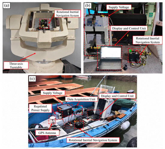
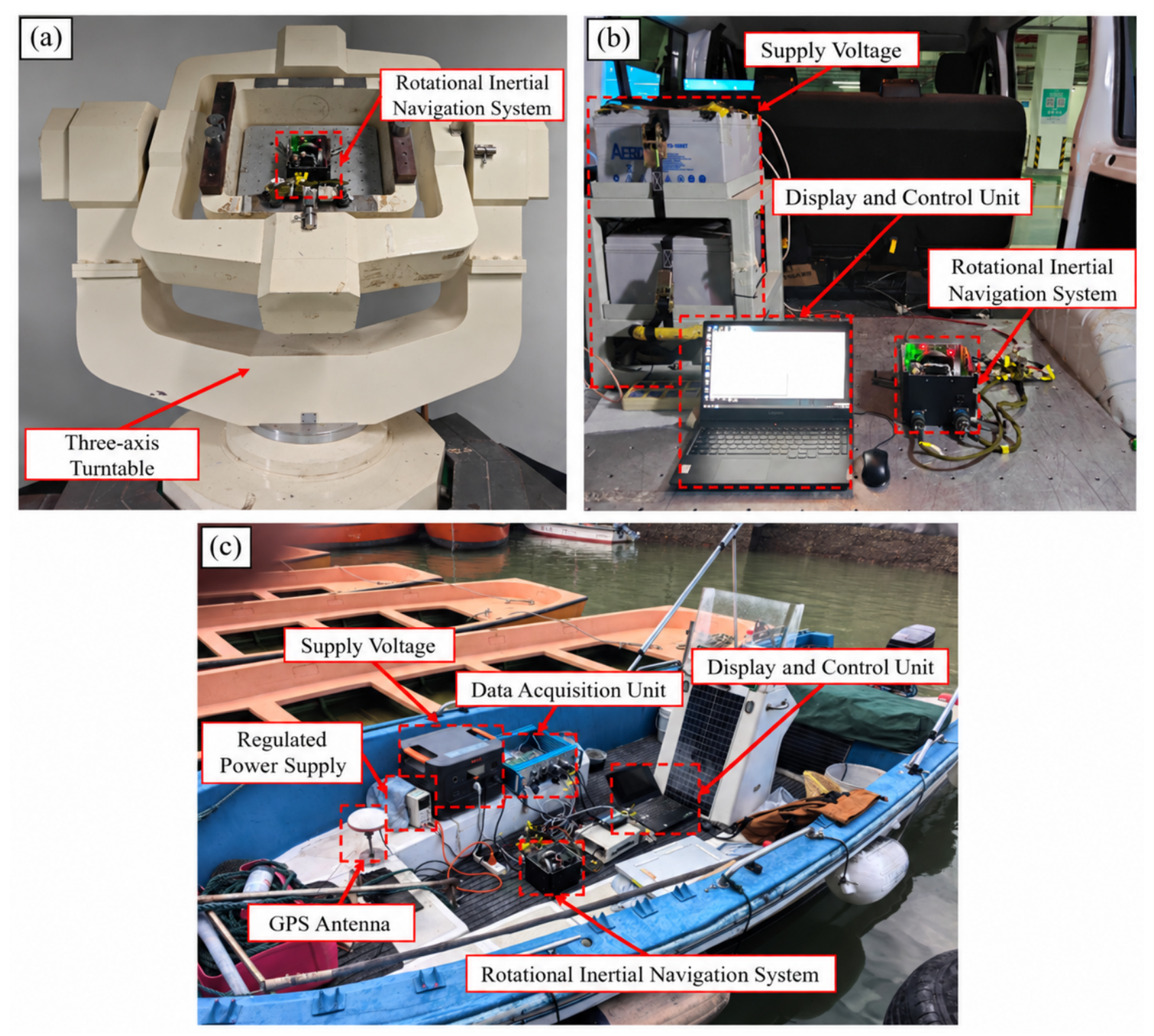
The static eight-position experiment was conducted to evaluate heading repeatability under different initial headings. The vehicle-mounted experiment was designed to assess the system’s sensitivity to nonperiodic road irregularities, acceleration, braking, and turning maneuvers. The shipboard experiment was performed to validate the proposed method under real-world marine motion conditions by comparing the primary navigation outputs with synchronized GNSS positions and reference attitude measurements. Figure 1 illustrates the corresponding experimental setups and deployment scenarios. The main hardware components and experimental parameters of the three experiments are summarized in Table 1. In the vehicle-mounted experiment, the conventional error-state Kalman filter based on instantaneous velocity/position matching was compared with the complete processing framework we propose.

Figure 1. Test and deployment platforms: (a) static eight-position test; (b) vehicle-based dynamic test; (c) shipboard deployment context for the retained navigation record.

Table 1. Experimental hardware and configuration summary.

Item	Specification
Gyroscope bias	0.003°/h
Accelerometer bias	10μg
IMU sampling rate	200 Hz
GNSS receiver	CUAV C-RTK 9Ps (u-blox ZED-F9P); update rate 20 Hz
Reference attitude system	INS/GNSS integrated system; heading accuracy 0.008°
Reference turntable	Position accuracy ±3′′, rate resolution 0.001°/s
Time synchronization	GNSS 1PPS signal with timestamp alignment

5.1. Static Eight-Position Alignment Repeatability Test

5.1.1. Test Procedure

The dual-axis RINS was set in turn to initial headings of 0°, 45°, 90°, 135°, 180°, −135°, −90°, and −45°, and four independent alignments were run at each, 32 in all. What is being measured here is stability from one run to the next at a fixed heading, so the figures that matter are the peak-to-peak spread and the sample standard deviation of the four results at each position.

5.1.2. Repeatability at Different Initial Headings

Table 2 lists the raw heading-alignment results for the 32 static tests. Table 3 summarizes the mean heading deviation, peak-to-peak spread, sample standard deviation, and two-sided 95% confidence-interval half-width at each initial heading. With four repetitions per heading, the half-width was calculated using $t_{0.975,3}=3.182$.

Table 2. Raw heading-alignment results for 32 static eight-position tests.

Initial Heading	Trial 1 (°)	Trial 2 (°)	Trial 3 (°)	Trial 4 (°)
0°	−0.6900	−0.6958	−0.6845	−0.6845
45°	44.2905	44.2863	44.2896	44.2905
90°	89.2950	89.2860	89.2954	89.2901
135°	134.3096	134.3219	134.3078	134.3098
180°	179.3395	179.3333	179.3250	179.3276
−135°	−135.6656	−135.6671	−135.6528	−135.6534
−90°	−90.6561	−90.6601	−90.6644	−90.6644
−45°	−45.6842	−45.6847	−45.6760	−45.6849

Table 3. Heading-alignment repeatability in the static eight-position test.

Initial Heading	Mean Heading Deviation (°)	Peak-to-Peak (°)	Standard Deviation (°)	95% CI Half-Width (°)
0°	−0.6887	40.68	19.43	30.91
45°	−0.7108	15.12	7.18	11.42
90°	−0.7084	33.84	16.05	25.53
135°	−0.6877	50.76	23.33	37.12
180°	−0.6687	52.20	23.20	36.91
−135°	−0.6597	51.48	27.64	43.98
−90°	−0.6612	29.88	14.35	22.83
−45°	−0.6824	32.04	15.52	24.69

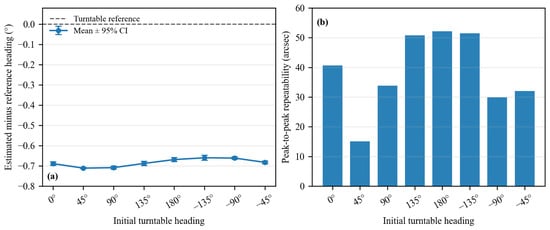
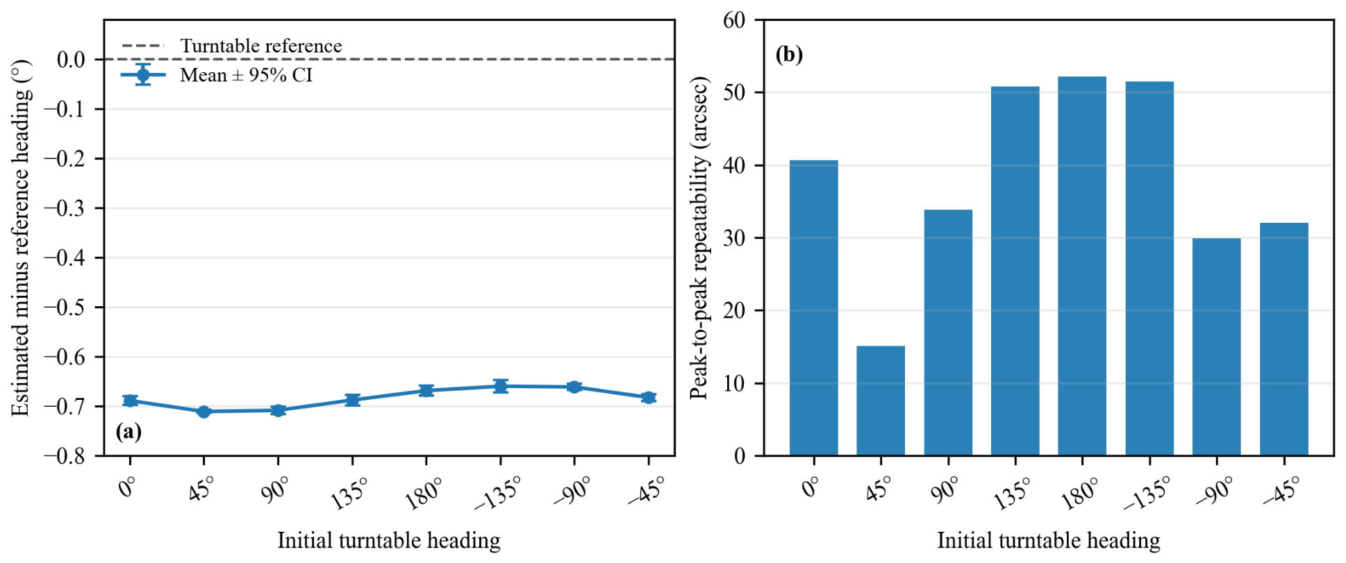
Table 3 collects the mean heading deviation, peak-to-peak spread, and sample standard deviation obtained from the four tests at each position in Table 2. All eight positions sit about −0.68° from their nominal turntable heading, by very nearly the same amount, which points to a fixed difference between the installation zero of the system and the reference heading rather than to an error of the algorithm.

Peak-to-peak repeatability at a single position ranges from 15.12′′ to 52.20′′ and averages 38.25′′ (Table 3 and Figure 2). No gross divergence occurred in the four runs at any heading. The wide confidence intervals at several positions, however, reflect the small sample and limit the strength of the statistical conclusion.

Figure 2. Static eight-position validation against the turntable reference: (a) mean heading error with two-sided 95% confidence intervals; (b) peak-to-peak heading repeatability.

5.2. Vehicle-Based Dynamic Disturbance Test

5.2.1. Objective and Procedure

In the vehicle test, nonperiodic dynamic disturbances were imposed through road roughness, acceleration, braking, and cornering. Under identical equipment configuration, initial heading, and alignment duration, seven independent runs were conducted with each of the conventional error-state EKF and the proposed pipeline, both against a 50 mil heading reference, to evaluate the alignment accuracy of the proposed method.

As shown in Table 4, against the 50 mil heading reference, the conventional method yields a heading RMSE of 0.3076 mil, while the proposed method achieves 0.1347 mil, a reduction of 56.2%.

Table 4. Heading-alignment results for two independent seven-run vehicle series.

Test No.	Conventional Error-State EKF (°)	Proposed Pipeline (°)
1	50.15	50.06
2	49.75	49.89
3	49.68	49.85
4	50.42	50.16
5	50.36	50.18
6	49.73	49.87
7	50.31	50.13
RMSE	0.3076	0.1347

5.2.2. Heading-Alignment Accuracy and Repeatability Analysis

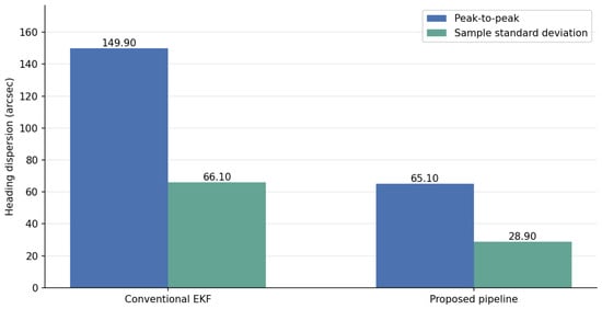
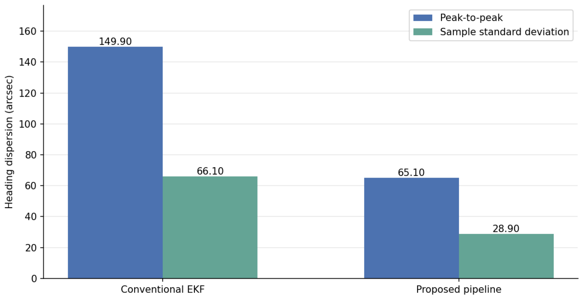
From the two seven-run series in Table 4, against the 50 mil heading reference, the conventional method yields a heading RMSE of 0.3076 mil, while the proposed method achieves 0.1347 mil, a reduction of 56.2%. In terms of within-series repeatability, the conventional method shows a peak-to-peak heading spread of 149.9′′ and a sample standard deviation of 66.1′′, against 65.1′′ and 28.9′′ for the proposed method—reductions of about 56.5% and 56.2%, respectively (Table 5 and Figure 3).

Table 5. Within-series heading repeatability in the vehicle-based dynamic test.

Method	Heading Peak-to-Peak (′′)	Standard Deviation (′′)	Peak-to-Peak Improvement	Standard-Deviation Improvement
Conventional error-state EKF	149.9	66.1	—	—
Proposed method	65.1	28.9	56.5%	56.2%

Figure 3. Within-series heading-dispersion metrics for the conventional EKF and proposed pipeline.

The vehicle-based dynamic test shows that, under the conditions of this experiment, the proposed pipeline yields both smaller within-series heading dispersion and smaller deviation from the reference than the conventional error-state EKF.

5.3. Shipborne Navigation Experiment

5.3.1. Test Conditions and Measured Ship-Motion Characteristics

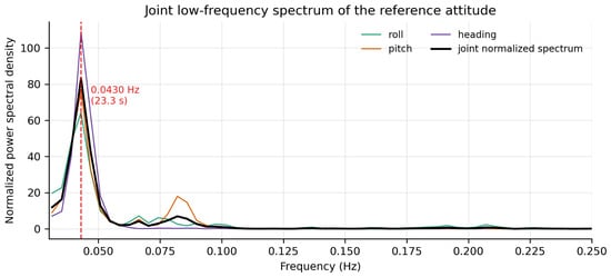
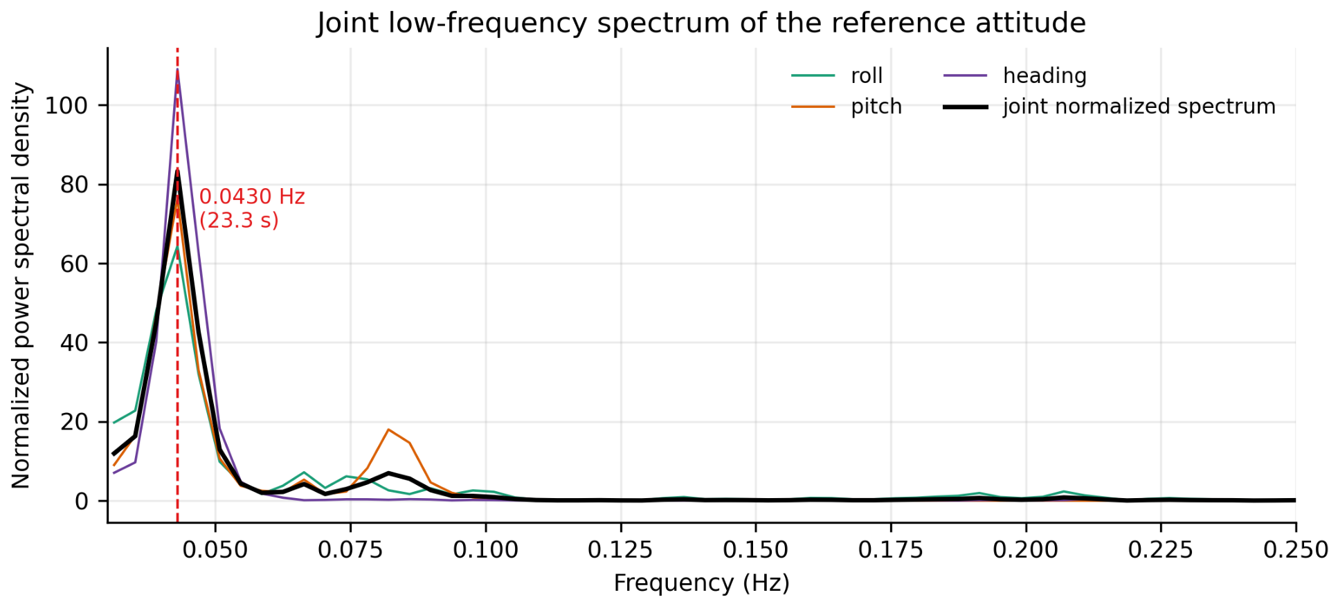
The shipborne test was conducted under moored conditions (berth coordinates 31.248921° N, 121.495713° E). The dual-axis RINS was installed inside the cabin and the GNSS antenna on the upper deck, with a fixed lever arm between them. During mooring, wind, waves, and current kept the hull rolling, pitching, and yawing at low frequencies, while its center of mass barely translated; the measured GNSS positions remained in the vicinity of the berth throughout, which represents a typical low-translational moored condition. After removing the mean and linear trend from the recorded reference attitude data, the power spectra of the roll, pitch, and heading channels were computed using the Welch method with 256 s Hann-window segments and 50% overlap. The spectrum of each axis was first normalized by its integrated power within the 0.03–0.25 Hz band, and the three spectra were then averaged, so that the axis with the largest motion amplitude would not dominate the joint spectral estimate. As shown in Figure 4, the principal component of the joint attitude spectrum is located at 0.0430 Hz, corresponding to a period of 23.3 s; a weaker spectral lobe appears near twice this frequency, indicating that the measured ship motion consists of a dominant fundamental component together with smaller harmonic components. It should be noted that the spectral analysis only confirms the presence of an identifiable dominant period in the ship motion, which provides measured evidence for selecting the frequency-adaptive integration window in the proposed method; the effectiveness of the method itself is examined by the navigation results in Section 5.3.2.

Figure 4. Normalized joint spectrum of the reference roll, pitch, and heading recorded in the shipborne test interval. The red dashed vertical line marks the dominant frequency at 0.0430 Hz, corresponding to a period of 23.3 s.

5.3.2. Long-Duration Pure Inertial Navigation Results with Different Alignment Methods

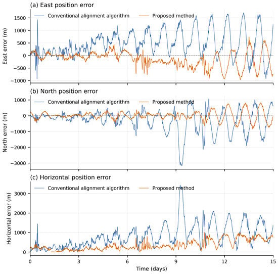
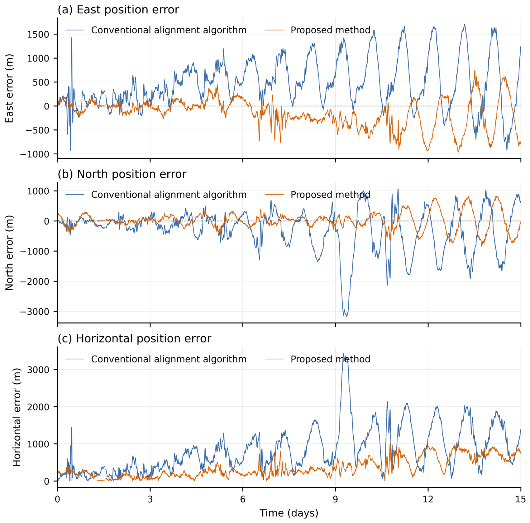
To examine the influence of initial alignment quality on subsequent navigation, the dual-axis RINS was switched to pure inertial navigation mode after initial alignment by the conventional alignment algorithm and by the proposed method, respectively, and ran continuously for 15 days without any external corrections. Position errors were computed against the berth position provided by the GNSS as the ground truth. Figure 5 shows the time histories of the east, north, and horizontal position errors corresponding to the two alignment methods, and Table 6 summarizes the error statistics.

Figure 5. Time histories of the (a) east, (b) north, and (c) horizontal position errors of 15-day pure inertial navigation with the two alignment methods.

Table 6. Position-error statistics of 15-day pure inertial navigation with the two alignment methods.

Algorithm	East RMSE (m)	North RMSE (m)	Horizontal RMSE (m)	Horizontal P95 (m)	Horizontal Max (m)
Conventional alignment	697.39	762.09	1033.02	1912.21	3438.69
Proposed method	333.65	282.58	437.23	851.87	1011.30

As shown in Table 6, the proposed method yields east, north, and horizontal position RMSEs of 333.65 m, 282.58 m, and 437.23 m, respectively, reductions of 52.2%, 62.9%, and 57.7% compared with the conventional alignment algorithm. The 95th percentile of the horizontal position error decreases from 1912.21 m to 851.87 m (a reduction of 55.5%), and the maximum from 3438.69 m to 1011.30 m (a reduction of 70.6%). The two methods share the same inertial hardware, the same recorded dataset, and an identical pure inertial navigation solver; the only difference lies in the initial alignment stage. The marked difference in navigation errors can therefore be attributed to the improved initial alignment accuracy: initial attitude and heading errors are the dominant drivers of position drift in pure inertial navigation, and reducing the alignment error directly suppresses the accumulation of long-duration navigation errors. Moreover, as shown in Figure 5, the error curves of the proposed method remain below those of the conventional method throughout the 15 days and grow more gently, further demonstrating that the proposed alignment framework achieves higher-quality initial alignment under real shipborne disturbance conditions. The shipborne test leads to the following results. First, the measured moored-ship motion exhibits a clearly identifiable dominant period (0.0430 Hz, 23.3 s), which is consistent with the low-frequency quasi-periodic marine motion characteristics targeted by the proposed method; the prerequisite for the frequency-adaptive integration window and the harmonic reconstruction is thus supported by measured data. Second, with identical hardware, identical data, and an identical navigation solver, the proposed alignment method reduces the horizontal position RMSE of 15-day pure inertial navigation from 1033.02 m to 437.23 m (a reduction of 57.7%) and the maximum horizontal error from 3438.69 m to 1011.30 m (a reduction of 70.6%), demonstrating that the proposed alignment framework effectively improves initial alignment quality in a real shipborne environment.

6. Conclusions

We propose an initial alignment framework that integrates encoder-aided compensation for mechanism-induced angular velocity, multi-axis dominant frequency estimation, phase-preserving harmonic reconstruction, dynamic lever-arm velocity transfer, period-matched integral measurements, and component-wise robust error-state filtering. A total of 32 static trials conducted at eight different headings yielded peak-to-peak heading repeatability ranges of 15.12′′–52.20′′, with the uncertainty associated with only four repeated trials per heading explicitly reported. In vehicle-mounted experiments against a known 50 mil heading reference, the proposed framework reduced the heading RMSE from 62.3′′ to 27.3′′ and the within-series peak-to-peak spread from 149.9′′ to 65.1′′ compared with the conventional error-state Kalman filter, both by about 56%. In the shipborne experiment, the dominant component of the joint attitude spectrum of the moored vessel was identified at 0.0430 Hz (23.3 s), consistent with the low-frequency quasi-periodic motion assumed by the method; with identical hardware, identical data, and an identical pure inertial navigation solver, the alignment produced by the proposed framework reduced the horizontal position RMSE of 15-day pure inertial navigation from 1033.02 m to 437.23 m (a reduction of 57.7%) and the maximum horizontal error from 3438.69 m to 1011.30 m (a reduction of 70.6%) relative to the conventional alignment algorithm. These results demonstrate that the proposed framework improves initial alignment quality under static, vehicle-mounted, and moored shipborne conditions, and that the improvement propagates into a substantial reduction of long-duration navigation errors.

References

- Titterton, D.H.; Weston, J.L. Strapdown Inertial Navigation Technology, 2nd ed.; IET: Stevenage, UK, 2004. [Google Scholar]
- Groves, P.D. Principles of GNSS, Inertial, and Multisensor Integrated Navigation Systems, 2nd ed.; Artech House: Boston, MA, USA, 2013. [Google Scholar]
- Farrell, J.A. Aided Navigation: GPS with High Rate Sensors; McGraw-Hill: New York, NY, USA, 2008. [Google Scholar]
- Savage, P.G. Strapdown Analytics; Strapdown Associates: Maple Plain, MN, USA, 2000. [Google Scholar]
- Gao, W.; Zhang, Y.; Wang, J. Research on Initial Alignment and Self-Calibration of Rotary Strapdown Inertial Navigation Systems. Sensors 2015, 15, 3154–3171. [Google Scholar] [CrossRef] [Scilit] [PubMed]
- Ren, Q.; Wang, B.; Deng, Z.; Fu, M. A Multi-Position Self-Calibration Method for Dual-Axis Rotational Inertial Navigation System. Sens. Actuators A Phys. 2014, 219, 24–31. [Google Scholar] [CrossRef] [Scilit]
- Zhang, Q.; Wang, L.; Liu, Z.; Feng, P. An Accurate Calibration Method Based on Velocity in a Rotational Inertial Navigation System. Sensors 2015, 15, 18443–18458. [Google Scholar] [CrossRef] [Scilit] [PubMed]
- Sun, X.; Lai, J.; Lyu, P.; Liu, R.; Gao, W. A Fast Self-Calibration Method for Dual-Axis Rotational Inertial Navigation Systems Based on Invariant Errors. Sensors 2024, 24, 597. [Google Scholar] [CrossRef] [Scilit] [PubMed]
- Bai, S.; Lai, J.; Lyu, P.; Xu, X.; Liu, M.; Huang, K. A System-Level Self-Calibration Method for Installation Errors in a Dual-Axis Rotational Inertial Navigation System. Sensors 2019, 19, 4005. [Google Scholar] [CrossRef] [Scilit] [PubMed]
- Guan, B.; Liu, Z.; Wei, D.; Fu, Q. Design of a Multi-Position Alignment Scheme. Sensors 2024, 24, 1938. [Google Scholar] [CrossRef] [Scilit] [PubMed]
- Song, T.; Li, K.; Wang, L.; Sui, J.; Wang, L. A Rapid and High-Precision Initial Alignment Scheme for Dual-Axis Rotational Inertial Navigation System. Microsyst. Technol. 2017, 23, 5515–5525. [Google Scholar] [CrossRef] [Scilit]
- Wei, D.; Li, S.; Fu, Q. A New Initial Alignment Scheme for Dual-Axis Rotational Inertial Navigation System. IEEE Trans. Instrum. Meas. 2022, 71, 8503010. [Google Scholar] [CrossRef] [Scilit]
- Fossen, T.I. Handbook of Marine Craft Hydrodynamics and Motion Control, 2nd ed.; Wiley: Hoboken, NJ, USA, 2021. [Google Scholar]
- Rogers, R.M. Applied Mathematics in Integrated Navigation Systems, 3rd ed.; American Institute of Aeronautics and Astronautics: Reston, VA, USA, 2007. [Google Scholar]
- Seo, J.; Lee, H.K.; Lee, J.G.; Park, C.G. Lever Arm Compensation for GPS/INS/Odometer Integrated System. Int. J. Control Autom. Syst. 2006, 4, 247–254. [Google Scholar]
- Cao, Q.; Zhong, M.; Zhao, Y. Dynamic Lever Arm Compensation of SINS/GPS Integrated System for Aerial Mapping. Measurement 2015, 60, 39–49. [Google Scholar] [CrossRef] [Scilit]
- Maybeck, P.S. Stochastic Models, Estimation, and Control; Academic Press: New York, NY, USA, 1979; Volume 1. [Google Scholar]
- Huber, P.J.; Ronchetti, E.M. Robust Statistics, 2nd ed.; Wiley: Hoboken, NJ, USA, 2009. [Google Scholar]
- Zheng, Z.; Han, S.; Zheng, K. An Eight-Position Self-Calibration Method for a Dual-Axis Rotational Inertial Navigation System. Sens. Actuators A Phys. 2015, 232, 39–48. [Google Scholar] [CrossRef] [Scilit]
- Li, J.; Su, L.; Wang, F.; Li, K.; Zhang, L. An Improved Online Fast Self-Calibration Method for Dual-Axis RINS Based on Backtracking Scheme. Sensors 2022, 22, 5036. [Google Scholar] [CrossRef] [Scilit] [PubMed]
- Jiang, R.; Yang, G.; Zou, R.; Wang, J.; Li, J. Accurate Compensation of Attitude Angle Error in a Dual-Axis Rotation Inertial Navigation System. Sensors 2017, 17, 615. [Google Scholar] [CrossRef] [Scilit] [PubMed]
- Xing, H.; Chen, Z.; Yang, H.; Wang, C.; Lin, Z.; Guo, M. Self-Alignment MEMS IMU Method Based on the Rotation Modulation Technique on a Swing Base. Sensors 2018, 18, 1178. [Google Scholar] [CrossRef] [Scilit] [PubMed]
- Fan, Z.; Chai, H.; Liang, X.; Wang, H. Experimental Research on Shipborne SINS Rapid Mooring Alignment with Variance-Constraint Kalman Filter and GNSS Position Updates. Sensors 2024, 24, 3487. [Google Scholar] [CrossRef] [Scilit] [PubMed]
- Yao, P.; Yang, G.; Peng, X. An Alignment Method Based on KF-ASMUKF Hybrid Filtering for Ship’s SINS under Mooring Conditions. Sensors 2021, 21, 7104. [Google Scholar] [CrossRef] [Scilit] [PubMed]
- Tang, J.; Bian, H.; Ma, H.; Wang, R. One-Step Initial Alignment Algorithm for SINS in the ECI Frame Based on the Inertial Attitude Measurement of the CNS. Sensors 2022, 22, 5123. [Google Scholar] [CrossRef] [Scilit] [PubMed]
- Liu, C.; Li, D.; Li, H.; Lan, T.; Lou, Q.; Wei, G.; Gao, C.; Tian, M.; Tan, Z.; Yu, X. A Group Affine-Based Inverse Alignment Method for High-Precision Rotational Inertial Navigation Systems. Sensors 2025, 25, 1767. [Google Scholar] [CrossRef] [Scilit] [PubMed]
- Su, E.; Wang, J.; Sheng, W.; Mou, Y.; Li, T.; Liu, J. Single-Axis Rotational Inertial Navigation Systems for USVs: A Review of Key Technologies. Micromachines 2026, 17, 557. [Google Scholar] [CrossRef] [Scilit] [PubMed]
- Wen, Z.; Cai, Q.; Yang, G. Modeling and Analysis of the Angular Velocity Phase-Based Lever Arm Effect in the Self-Calibration Process of Fixed-Wing Airborne Dual-Axis RINS. Measurement 2025, 254, 117632. [Google Scholar] [CrossRef] [Scilit]
- Wu, Q.; Li, K.; Song, T. The Calibration for Inner and Outer Lever-Arm Errors Based on Velocity Differences of Two RINSs. Mech. Syst. Signal Process. 2021, 160, 107868. [Google Scholar] [CrossRef] [Scilit]
- Song, T.; Li, K.; Sui, J.; Liu, Z.; Liu, J. Self-Calibration Method of the Inner Lever-Arm Parameters for a Tri-Axis RINS. Meas. Sci. Technol. 2017, 28, 115105. [Google Scholar] [CrossRef] [Scilit]
Disclaimer/Publisher’s Note: The statements, opinions and data contained in all publications are solely those of the individual author(s) and contributor(s) and not of MDPI and/or the editor(s). MDPI and/or the editor(s) disclaim responsibility for any injury to people or property resulting from any ideas, methods, instructions or products referred to in the content. |
© 2026 by the authors. Licensee MDPI, Basel, Switzerland. This article is an open access article distributed under the terms and conditions of the Creative Commons Attribution (CC BY) license.