Nonlinear Model Predictive Control of Process Water Quality in the Closed-Loop Water Circuit of the Aktogai GOK Flotation Plant

Abstract

This paper presents a simulation-based feasibility study of nonlinear model predictive control (NMPC) for process water quality management in the closed-loop water circuit of the Aktogai copper concentrator. Repeated water recirculation leads to the accumulation of total dissolved solids (TDSs), organic compounds (CODs), and suspended solids (TSSs), degrading flotation efficiency. A dynamic model of the process water pond with nine flows is combined with pseudo-first-order kinetics for H₂O₂ oxidation (k_ox = 0.003 L/(mg·h)) and polyaluminum chloride (PAC)/FeCl₃ coagulation (k_coag = 0.005 L/(mg·h)). The NMPC manipulates the treated-effluent flow Q₂ and the coagulant and oxidant doses over an 8 h prediction horizon, uses normalized one-sided soft constraints on water quality and a reagent cost, and is solved through sequential quadratic programming. The volume, TDSs, and TSSs are assumed to be measured online, whereas CODs are available only from laboratory analyses taken every 2–8 h with a 2 h delay. NMPC was compared with no-control, fixed dosing, a maximum-dilution policy, and a proportional–integral (PI) feedback dosing benchmark with the same manipulated variables. Under nominal disturbances, all strategies met the process limits. Under a simulated stress-test scenario (ore change and reagent overdosing), no control produced 26, 37, and 25 h of TDS, COD, and TSS violations in 72 h; maximum dilution alone removed the TDS and TSS violations but left 13 h of COD violations. With online measurements, a well-tuned PI controller performed almost as well as NMPC (1 h vs. 0 h of COD violations). With laboratory COD analyses, the PI controller incurred 4–11 h of COD violations, whereas NMPC, using a model-based COD estimate between analyses, incurred none, at the cost of 9–47% higher oxidant consumption; this advantage reflects the combined effect of model-based COD estimation and predictive optimization, not of predictive optimization alone. It persisted under up to 30% adverse parametric plant–model mismatch, and the results were insensitive to tenfold variations in the selected NMPC tuning weights. TDSs could be held below their limit only through hydraulic dilution and only while the thickener-overflow TDSs remained below about 2260 mg/L.

1. Introduction

Industrial water use is increasingly shifting towards circular, closed-loop practices [1] in response to growing water scarcity [2]. The mining industry is one of the largest industrial consumers of water resources, accounting for 2–4.5% of national water consumption in resource-extracting economies [3,4]. In the closed-loop water circuits of concentrators, water is repeatedly returned to the process cycle, causing the cumulative accumulation of dissolved mineral salts, flotation reagents, and suspended particles [3,4,5].

Aktogai Mining and Processing Plant (Aktogai GOK, from the Russian abbreviation for mining and processing plant; KAZ Minerals Aktogay LLP, Aktogay, Kazakhstan) operates on a porphyry copper deposit and is one of the largest mining enterprises in Central Asia [6,7,8]. The specific mineral composition of the ore [9] causes heightened sensitivity of the water circuit to seasonal and process disturbances.

Under repeated recirculation in the water circuit, the progressive accumulation of dissolved mineral salts (TDSs), residual flotation reagents (CODs), and fine suspended particles (TSSs) occurs. Increased ionic strength and TDSs alter collector adsorption conditions on mineral surfaces; rising TSSs degrade hydrodynamics in flotation cells; increasing organic load CODs disrupt froth stability and reduce separation selectivity [7,10,11,12,13,14]. At the Aktogai plant, the collector SIBX (sodium isobutyl xanthate), sodium thiosulfate, thickener flocculant, and antiscalant are used [15]—combined accumulation of residues from these reagents is the primary source of organic load. A significant operational problem is that water quality changes considerably faster than periodic laboratory monitoring is performed, as confirmed via an analysis of challenges in mining process water quality assessments [16].

Traditional water circuit management methods focus on hydraulic parameter regulation and do not account for water quality dynamics, although the need for a systematic approach to process water quality management in concentrators was established by Levay and Schumann (2006) [17]. Noome (2023) investigates nonlinear model predictive control (NMPC) for grinding and flotation process control with an emphasis on reducing computational load—the water circuit and TDS/COD/TSS indicators are not control objects [18]. Quintanilla et al. (2023–2024) developed economic model predictive control (E-MPC) for flotation cell control—the closed-loop water circuit, as a whole, is not considered [19,20], nor is it in the flotation control review by Shean and Cilliers (2011) [21]; see also the reviews of control methods in mineral processing [22] and flotation [23]. None of these approaches includes TDSs, CODs, and TSSs in the control system state vector.

The objective of this work is to assess, through simulation, whether incorporating process water quality indicators into the state vector of an NMPC system reduces violations of the process limits for TDSs, CODs, and TSSs compared with uncontrolled operation and with conventional feedback dosing, under a nominal disturbance scenario and a simulated stress-test scenario, with realistic measurement conditions (laboratory-based COD analysis). To achieve this objective, the following tasks were addressed:

• Develop a nonlinear dynamic model of the process water pond with nine flows, Q1–Q9, internal disturbance sources, and pseudo-first-order reagent kinetics;
• Formulate the NMPC problem with one-sided soft constraints on water quality, a reagent cost, and actuator bounds;
• Compare NMPC with no-control, fixed dosing, a maximum-dilution policy, and a proportional–integral (PI) feedback dosing benchmark over 72 h under a nominal scenario and a simulated stress-test scenario;
• Evaluate the effect of laboratory-based COD measurements, plant–model mismatch, and objective weights on closed-loop performance.

2. Materials and Methods

2.1. Plant Description—Aktogai GOK

The object of the study is the closed-loop process water circuit of the flotation plant at Aktogai GOK (KAZ Minerals Aktogay LLP, Aktogay, Kazakhstan). The Kyzylkiya deposit lies 2 km northeast of the Aktogai deposit [24], which is located about 25 km east of Aktogai station on the Almaty Railway [25]. The deposit is a porphyry copper body with hydrothermal alteration that causes variability in the ore mineral composition and, consequently, variable process water mineralization [9]. The plant processes porphyry copper ore via open-pit mining; the sulphide concentrator has a design capacity of 25 million tonnes of ore per year [25], and in 2021 the tailings volume at Aktogai was 27.5 million tonnes [6].

In 2021, KAZ Minerals deployed the artificial intelligence (AI)-based process optimization system TRIT-AI at Aktogai, trained on 500 million historical supervisory control and data acquisition (SCADA) data points, suggesting potential compatibility with advanced process control approaches such as NMPC, subject to further validation [6].

2.2. Mathematical Model of the Water Circuit

2.2.1. State Vector and Flows

System state vector:

$$x(t)={\left[\begin{array}{cccc}V\left(t\right)& \mathit{TDS}\left(t\right)& \mathit{COD}\left(t\right)& \mathit{TSS}\left(t\right)\end{array}\right]}^T$$

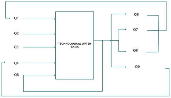
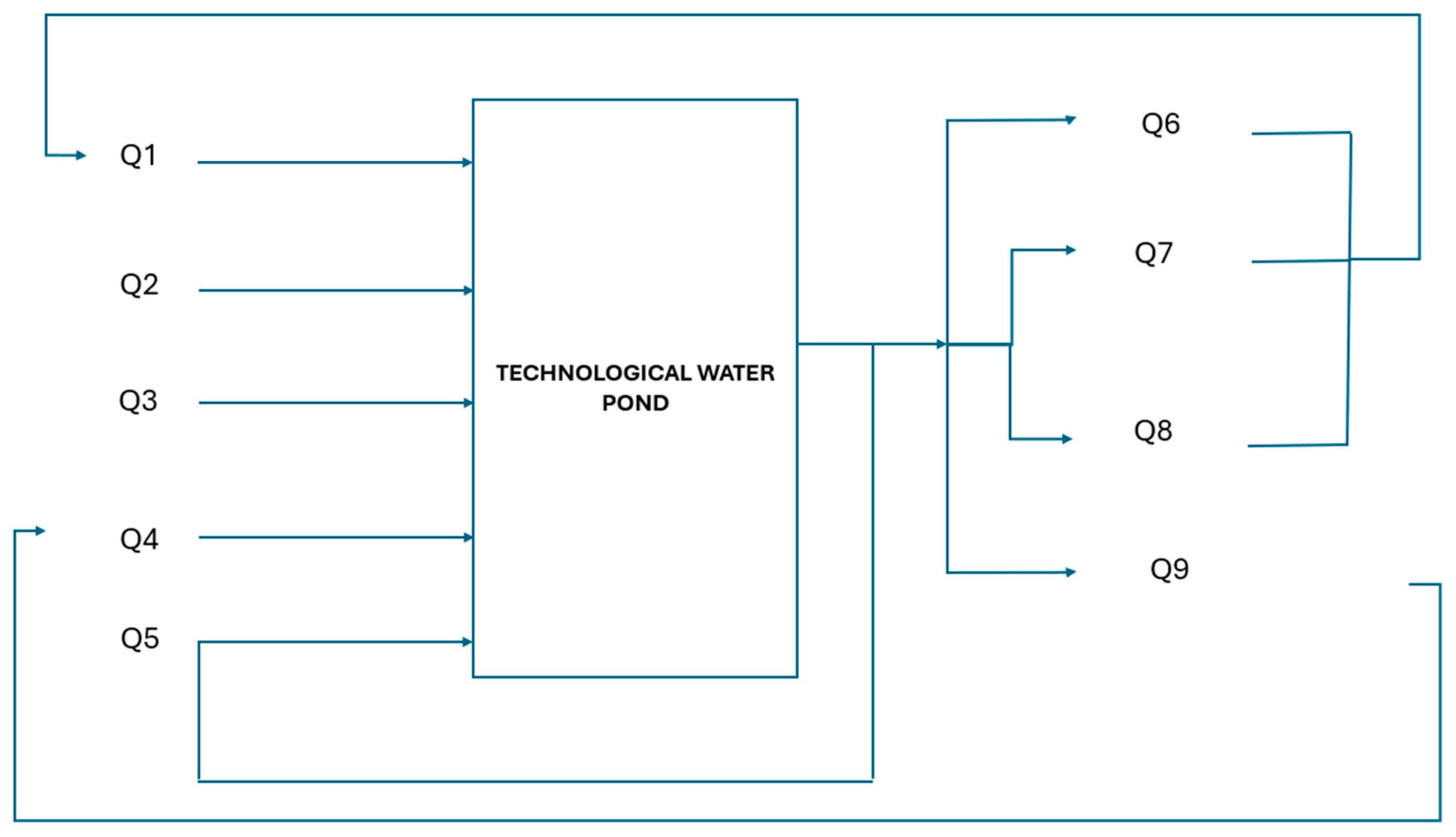
The process flowsheet includes five input flows (Q₁–Q₅) and four output flows (Q₆–Q₉).

The recirculation flow Q₅ is the part of the process–water pump discharge that is returned directly to the pond through the recirculation pipeline when plant demand falls below the minimum pump flow [15]. Because Q₅ is withdrawn from and returned to the same pond, its withdrawal and return cancel in both the volume and the quality balances: with the control volume drawn around the pond (Figure 1), Q₅ makes no net contribution to V, TDSs, CODs, or TSSs. It is therefore excluded from the balance equations and is not a manipulated variable. The outlet flows Q₆–Q₉ are the net deliveries to the process units; Q₁ is the return from the tailings thickener, and Q₄ is the return from the tailings storage facility (Figure 1).

Figure 1. Closed-loop process water circuit of Aktogai GOK with input flows Q1–Q5 and output flows Q6–Q9. Q₅ is the internal recirculation of pump discharge back to the pond and makes no net contribution to the pond balances.

The flow structure and nominal flow rates (Table 1) were adopted from the internal technical documentation of the Bozshakol concentrator [15]. The Aktogai and Bozshakol sulfide concentrators were developed by KAZ Minerals with similar design and engineering solutions and comparable processing equipment [26]; the Bozshakol data are therefore used as representative design values, because a corresponding document for Aktogai was not available to the authors. The model covers only the process water circuit of the sulfide concentrator; the oxide heap-leach and solvent extraction–electrowinning (SX-EW) circuit at Aktogai is not included.

Table 1. Process flows of the model.

Flow	Purpose	Flow Rate, m3/h	Mode
Q1	Tailings thickener overflow	3900	Constant
Q2	Treated industrial effluents	80–300 (nominal 120)	Manipulated variable
Q3	Raw water tank overflow	40	Constant
Q4	Supply from tailings storage facility	500/0	On when V < Vmin; off when V > Vmin + 150 m3
Q5	Internal recirculation of pump discharge	150/350	No net effect on the pond (not modelled)
Q6	Supply to grinding	1650	Constant
Q7	Supply to flotation	1900/2150	Before/after 24 h
Q8	Supply to tailings storage facility	450	Constant
Q9	Supply to thickening	300	Constant

The quality of input flows (TDS_i, COD_i, TSS_i, mg/L) was adopted from data reported for analogous porphyry copper processing plants [10,15] (unpublished); they are listed in Table 2.

Table 2. Quality of input flows.

Flow	TDSs, mg/L	CODs, mg/L	TSSs, mg/L
Q1–thickener overflow	2200	120	90
Q2–industrial effluents	700	30	20
Q3–tank overflow	500	10	10
Q4–tailings storage	1800	80	100
Q5–recirculation	=TDS (t)	=COD (t)	=TSS (t)

2.2.2. Water Balance Equation

$${\displaystyle \frac{\mathit{dV}}{\mathit{dt}}}=\left(Q_1+Q_2+Q_3+Q_4\right)-\left(Q_6+Q_7+Q_8+Q_9\right)$$

Constraints: V_min = 4700 m³, V_max = 6500 m³; initial volume V₀ = 5000 m³. The inflow from the tailings storage facility, Q₄ = 500 m³/h, is a level safeguard independent of the controller: it is switched on when V < V_min and off when V > V_min + 150 m³ (hysteresis). With the flows of Table 1, the inflow without Q₄ (at most 4240 m³/h) is lower than the outflow (4300 m³/h for t < 24 h and 4550 m³/h afterwards). The pond level is therefore sustained structurally by Q₄, and none of the manipulated variables can hold V above V_min indefinitely.

2.2.3. TDS Dynamics

$${\displaystyle \frac{d\left(\mathit{TDS}\right)}{\mathit{dt}}}={\displaystyle \frac{{\displaystyle {\sum }_{i=1}^n}{Q}_i\left({\mathit{TDS}}_i-\mathit{TDS}\right)+G_{\mathit{TDS}}}{V}}$$

With flows Q in m³/h, concentrations in mg/L, and volume V in m³, each flow term Q_i(C_i − C)/V is in mg/(L·h), and the source terms G carry units of m³·mg/(L·h) = g/h; the sum runs over the inflows Q₁–Q₄. The nominal TDS source G_TDS = 2.0 × 10⁵ g/h (200 kg/h) represents the leaching of soluble salts from ore and process products [27,28]; at the design throughput of 25 Mt of ore per year (≈2900 t/h) [25], this corresponds to about 0.07 kg of dissolved salts per tonne of ore. At the nominal operating point (V = 5000 m³, TDS = 1500 mg/L), the inflow Q₁ (TDS₁ = 2200 mg/L) contributes Q₁(TDS₁ − TDS)/V = 3900 × 700/5000 ≈ 546 mg/(L·h), and the source contributes G_TDS/V = 40 mg/(L·h). The hydraulic residence time V/ΣQ_out ≈ 1.2 h is short, so pond TDSs approach the flow-weighted inlet concentration within 1–2 h (see Section 3.1). In the steady state without Q₄, TDS = (ΣQ_iTDS_i + G_TDS)/ΣQ_i ≈ 2188 mg/L for Q₂ = 120 m³/h and ≈ 2125 mg/L for Q₂ = 300 m³/h, i.e., TDSs can be influenced only by the dilution and only within a narrow range. During disturbance scenario S₂ (t ∈ [20, 45] h), the source intensity increases by a factor of 1.35, consistent with TDS increases under ore composition changes [9].

2.2.4. COD Dynamics

The kinetic term k_COD·COD (k_COD = 0.012 h⁻¹) reflects the biological and chemical decomposition of organic compounds in process water. The internal source G_COD = 1.0 × 10⁴ g/h is formed by residual flotation reagents. Under disturbance scenario S₃ (t ≥ 35 h), the source intensity increases by a factor of 2.0, simulating increased reagent loading. The model incorporates chemical oxidation by H₂O₂ (manipulated variable u_ox, mg/L):

$${\displaystyle \frac{\mathit{dCOD}}{\mathit{dt}}}={\displaystyle \frac{\sum _i{Q}_i\left(\mathit{CO}{D}_i-\mathit{COD}\right)+G_{\mathit{COD}}}{V}}-k_{\mathit{COD}}\cdot \mathit{COD}-k_{\mathit{ox}}\cdot u_{\mathit{ox}}\cdot \mathit{COD}$$

where k_ox = 0.003 L/(mg·h) is an assumed pseudo-first-order oxidation coefficient, of the order reported for the H₂O₂-based (Fenton) oxidation of the organic load in wastewater [29]. It has not been identified for Aktogai process water and is therefore included in the plant–model mismatch analysis (Section 3.6). The manipulated variable u_ox is bounded:

0 ≤ u_ox ≤ 20 mg/L.

2.2.5. TSS Dynamics

$${\displaystyle \frac{\mathit{d}\left(\mathit{TSS}\right)}{\mathit{dt}}}={\displaystyle \frac{\sum _{\mathit{i}}{\mathit{Q}}_{\mathit{i}}\cdot (\mathit{TS}{\mathit{S}}_{\mathit{i}}-\mathit{TSS})+{\mathit{G}}_{\mathit{TSS}}}{\mathit{V}}}-{\mathit{k}}_{\mathit{s}}\cdot \mathit{TSS}$$

The settling coefficient k_s = 0.035 h⁻¹ was adopted for flotation tailings particles with d₈₀ < 25 μm (half-settling time τ_1/2 ≈ 19.8 h). Under disturbance scenario S₂ (t ∈ [20, 45] h), the source G_TSS increases by a factor of 1.5 due to degraded clarified water quality under a changed ore composition [9]. The extended model incorporates the coagulation by polyaluminum chloride (PAC)/FeCl₃ (control variable u_coag, mg/L):

$${\displaystyle \frac{\mathit{dTSS}}{\mathit{dt}}}={\displaystyle \frac{\sum _i{Q}_i\left(\mathit{TS}{S}_i-\mathit{TSS}\right)+G_{\mathit{TSS}}}{V}}-k_s\cdot \mathit{TSS}-k_{\mathit{coag}}\cdot u_{\mathit{coag}}\cdot \mathit{TSS}$$

where k_coag = 0.005 L/(mg·h) is an assumed pseudo-first-order coagulation coefficient, of the order consistent with reported coagulation kinetics of hydrolyzing metal salts [30]; like k_ox, it is included in the mismatch analysis (Section 3.6). The manipulated variable u_coag is bounded:

0 ≤ u_coag ≤ 15 mg/L

2.2.6. Numerical Implementation

The four ordinary differential equations are integrated with a fixed-step fourth-order Runge–Kutta method, with a sub-step of 0.1 h for the simulated plant and 0.25 h inside the NMPC prediction; the control interval is Δt = 1 h. All simulations were implemented in MATLAB (version R2020a; The MathWorks, Inc., Natick, MA, USA) with the Optimization Toolbox. No physical reagents, instruments, or samples were used in this study; the oxidant, the coagulants, and the flotation reagents are represented only as model inputs.

2.3. NMPC Problem Formulation

2.3.1. Cost Function

At each control step, the controller minimizes over the prediction horizon N_p = 8 h, a cost that penalizes only violations of water-quality alarm levels and limits (one-sided penalties); the reagent consumption and the input moves. Concentration set-points are not tracked, so cleaner water is never penalized. A similar soft-constraint structure has been used in water quality control problems [31,32]. With the manipulated variable vector u = [Q₂, u_coag, u_ox]^T and c ∈ {TDS, COD, TSS},

$$J={\displaystyle \sum _{i=1}^{N_p}}{\mathcal{l}}_i$$

$${\mathcal{l}}_i=w_{\mathrm{soft}}\sum _c{\left[\mathit{max}\left(0, {\displaystyle \frac{c_i-c_{\mathrm{soft}}}{c_{\max }}}\right)\right]}^2+w_{\mathrm{hard}}\sum _c{\left[\mathit{max}\left(0,{\displaystyle \frac{c_i-c_{\max }}{c_{\max }}}\right)\right]}^2$$

$$+w_V\left({\left[\mathit{max}\left(0, {\displaystyle \frac{V_{\min }-V_i}{1000}}\right)\right]}^2+{\left[\mathit{max}\left(0, {\displaystyle \frac{V_i-V_{\max }}{1000}}\right)\right]}^2\right)$$

$$+w_{\mathrm{coag}}{\displaystyle \frac{u_{\mathrm{coag},\mathrm{i}}}{15}}+w_{\mathrm{ox}}{\displaystyle \frac{u_{\mathrm{ox},\mathrm{i}}}{20}}+w_{\Delta u}{\displaystyle \sum _{j=1}^3}{\left({\displaystyle \frac{u_{j,i}-u_{j,i-1}}{u_{j,\mathit{max}}-u_{j,\mathit{min}}}}\right)}^2-w_{\mathrm{Q}2}{\displaystyle \frac{Q_{2,i}-Q_{2,\min }}{Q_{2,\max }-Q_{2,\min }}}$$

where c_soft = (2150, 112, 92) mg/L are the alarm levels and c_max = (2200, 120, 100) mg/L are the process limits for TDSs, CODs, and TSSs; V_min and V_max are the volume limits; u_j,max − u_j,min are the actuator ranges (Table 1 and Section 2.2.4 and Section 2.2.5); and w_soft = 10³, w_hard = 10⁵, w_V = 10³, w_coag = w_ox = 0.02, w_Δu = 0.05, and w_Q2 = 0.02 are dimensionless weights.

All terms are normalized by the corresponding limits or actuator ranges, so the weights do not depend on the physical units. The hard-limit and volume terms act as soft constraints, the alarm-level term creates a safety margin below the limits, the linear reagent terms penalize the chemical consumption, and the last term gives a small incentive to reuse treated effluent instead of discharging it. No volume set-point is tracked: because Q₅ is an internal recirculation, the pond level is governed by the Q₄ safeguard (Section 2.2.2), and the controller only keeps V within [V_min, V_max]. The sensitivity of the results to the weights is examined in Section 3.7.

The input sequence is parameterized by two move blocks: the first block covers the first hour, and the second holds the inputs constant over hours 2–8, giving six decision variables per step.

2.3.2. Optimization Solver and Constraint Handling

The optimization problem is solved at each step through sequential quadratic programming (SQP; MATLAB fmincon, SQP algorithm, at most 200 iterations, optimality tolerance 10⁻⁸). The actuator bounds (Table 1 and Section 2.2.4 and Section 2.2.5) are imposed directly as box constraints on the decision variables. The solver is warm-started from the shifted solution of the previous step; if it terminates without convergence (exit flag ≤ 0), it is restarted once from the mid-range point and the better of the two solutions is used. The first move of the returned sequence is always applied, and no fallback sequence is used. No guarantee of recursive feasibility or of soft-constraint satisfaction is claimed; solver statistics are reported in Section 3.7.

State constraints (TDS ≤ 2200 mg/L, COD ≤ 120 mg/L, TSS ≤ 100 mg/L, V_min ≤ V ≤ V_max) are enforced as soft constraints through the penalty terms of ℓ_i (Section 2.3.1).

The inflow Q₄ from the tailings storage facility is a level safeguard independent of the NMPC, consistent with the plant operating procedure [15]. Within the prediction, Q₄ may switch off when the predicted volume exceeds V_min + 150 m³ but is never predicted to switch on. This asymmetric treatment is a deliberate simplifying assumption of the prediction model. If the switch-on logic were included, the optimizer could lower Q₂ so that the predicted level falls below V_min and the safeguard water (TDS₄ = 1800 mg/L) dilutes the pond; the controller would then intentionally exploit Q₄, which lies outside its authority, as a dilution mechanism, and in preliminary simulations, this produced erratic control actions. Excluding the switch-on prevents this, at the price of a conservative prediction: when the safeguard is actually activated, the pond is diluted more than predicted. Because the inflow without Q₄ is structurally lower than the outflow (Section 2.2.2), Q₄ activation is an expected feature of operation and not a consequence of unmodeled disturbances.

2.3.3. Receding Horizon Algorithm

At each step, the controller (i) obtains the current measurements and the state estimate (Section 2.3.4); (ii) predicts the dynamics over N_p with the model of Section 2.2, holding all disturbances (internal sources, inlet concentrations, Q₇, and the Q₄ state) at their current values, i.e., without a preview of future disturbances; (iii) solves the optimization problem; and (iv) applies the first move [33]. This receding-horizon architecture corresponds to approaches used in water quality control for canals and polder networks [34,35].

2.3.4. Measurement Model and State Estimation

The pond volume, TDSs, and TSSs are assumed to be measured online every hour (level transmitter, conductivity, and turbidity sensors). CODs are available only from laboratory analysis: a sample is taken every T_S hours, and its result becomes available 2 h later; T_S = 2, 4, 6, and 8 h and the ideal case of hourly online COD measurements are considered. Between analyses, the NMPC estimates the current CODs by propagating the last available laboratory value with the nominal model and the inputs actually applied since the sampling instant (open-loop model-based estimator); volume, TDSs, and TSSs in the estimate are replaced by their online measurements. The plant is simulated with the same model structure; in the mismatch analysis (Section 3.6), the simulated plant uses perturbed parameters, while the controller keeps the nominal ones.

2.3.5. Benchmark Strategies

Four benchmarks with the same manipulated variables and actuator bounds are used: (i) no control (Q₂ = 120 m³/h, no reagents); (ii) fixed dosing (Q₂ = 120 m³/h, u_coag = 7.5 mg/L, u_ox = 10 mg/L); (iii) maximum dilution with fixed dosing (Q₂ = 300 m³/h, same doses), which isolates the hydraulic effect of Q₂; and (iv) maximum dilution with PI feedback dosing (Q₂ max + PI). In (iv), two independent PI loops set u_coag from the online TSS measurement and u_ox from the last available COD value (sample-and-hold), with set-points equal to the NMPC alarm levels (92 and 112 mg/L), proportional gain K_p = 2 (mg/L of reagent per mg/L of error), integral time T_i = 5 h, and conditional-integration anti-windup. K_p was selected by a trial from {0.5, 1, 2, 4} with online measurements in the stress scenario S4 and kept unchanged in all other cases.

2.4. Initial Conditions and Model Parameters

The initial conditions and the model parameters used in all simulations are summarized in Table 3. The kinetic coefficients and internal sources are discussed in Section 2.2.3, Section 2.2.4 and Section 2.2.5.

Table 3. Summary of model parameters.

Parameter	Symbol	Value	Unit
Initial water volume	V0	5000	m3
Min. volume	Vmin	4700	m3
Max. volume	Vmax	6500	m3
Initial TDSs	TDS0	1500	mg/L
Admissible TDSs	TDSmax	2200	mg/L
Initial CODs	COD0	80	mg/L
Admissible CODs	CODmax	120	mg/L
Initial TSSs	TSS0	120	mg/L
Admissible TSs	TSSmax	100	mg/L
COD degradation	kCOD	0.012	1/h
TSS settling	ks	0.035	1/h
TDS source	GTDS	2.0 × 105	g/h
COD source	GCOD	1.0 × 104	g/h
TSS source	GTSS	5.0 × 103	g/h
Simulation horizon	T	72	h

2.5. Disturbance Scenarios

Scenarios S2 and S3 represent disturbance types reported for the plant, whereas S4 is a simulation stress test: its disturbance amplitudes were chosen so that the process limits are actively threatened and are not derived from Aktogai operational data. Because all strategies satisfy the limits under the nominal scenario, the differences between the control strategies reported in Section 3 arise mainly under S4 and should be interpreted as a comparison under deliberately severe conditions. The disturbance scenarios and their model implementation are summarized in Table 4.

Table 4. Disturbance scenarios.

Scenario	Description	Model Implementation	Justification
S1–baseline	Normal operation, no additional disturbances	GTDS, GCOD, GTSS–baseline values	Typical Aktogai operating mode [6]
S2–rich ore	Increased impurity input (20–45 h): GTDS × 1.35; GTSS × 1.5	If 20 ≤ t ≤ 45 h	Ore composition change
S3–reagent loading (COD disturbance)	Increased reagent dosing (after 35 h): GCOD × 2.0	If t ≥ 35 h	Increased SIBX and depressant consumption [15]
S2 + S3–nominal	Simultaneous S2 and S3 disturbances	Both conditions active	Nominal scenario for controller comparison
S4–stress	S2 + S3 with degraded thickener overflow: TDS1 = 2250 mg/L, TSS1 = 110 mg/L, GTSS × 3.0 (20–45 h); COD1 = 132 mg/L (t ≥ 35 h)	Inlet concentrations of Q1 changed	Simulation stress test (amplitudes not derived from Aktogai data); limits actively threatened

Table 5 lists the manipulated variables with their bounds and the baseline values used in the benchmark strategies.

Table 5. Manipulated variables, bounds, and baseline values.

Variable	Lower Bound	Upper Bound	Baseline	Basis
Q2, m3/h	80	300	120	Treated-effluent flow; upper bound = assumed available effluent
ucoag, mg/L	0	15	0/7.5 (fixed dosing)	PAC/FeCl3 dosing range [30]
uox, mg/L	0	20	0/10 (fixed dosing)	H2O2 dosing range [29]
Q5, m3/h	—	—	150–350	Internal recirculation; not manipulated, no net effect

3. Results

3.1. Open-Loop System Dynamics (Baseline Model)

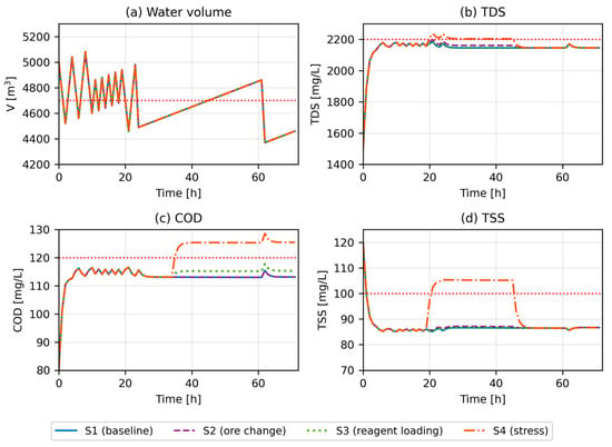
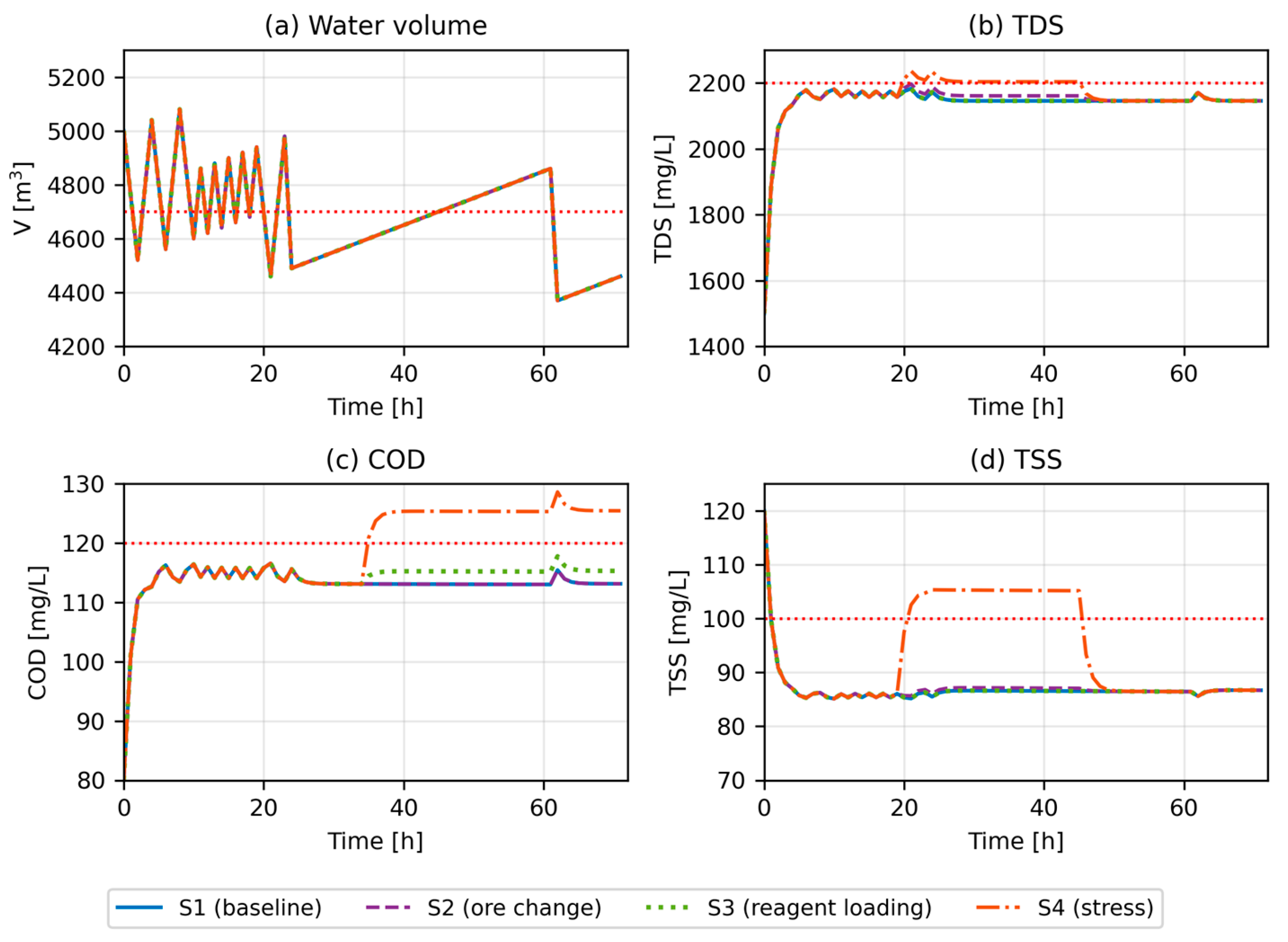
Figure 2 shows the open-loop response (Q₂ = 120 m³/h, no reagents) under the baseline S1, the individual disturbances S2 and S3, and the stress scenario S4.

Figure 2. Open-loop response (Q₂ = 120 m³/h, no reagents) under scenarios S1 (baseline), S2 (ore change), S3 (reagent loading), and S4 (stress); fourth-order Runge–Kutta (RK4) integration, 72 h. Red dotted lines—V_min and admissible limits. (a) Water volume; (b) TDSs; (c) CODs; (d) TSSs.

Because the hydraulic residence time is about 1.2 h, all quality indicators approach quasi-steady levels within a few hours, determined by the flow-weighted inlet concentrations, the internal sources, and the first-order removal terms; there is no slow monotonic accumulation over the 72 h horizon. Pond TDSs settle at about 2140–2190 mg/L, close to the limit, because the dominant inflow Q₁ carries 2200 mg/L. Scenario S2 raises TDSs by about 15 mg/L and S3 raises CODs by about 2 mg/L, without violating the limits. Under S4, TDSs, CODs, and TSSs exceed their limits (maxima of 2236, 128.6, and 105.3 mg/L). The sawtooth in the volume reflects the on/off operation of the Q₄ safeguard, and the change at t = 24 h is the increase in the flotation demand Q₇.

3.2. NMPC Performance

Table 6 compares the five strategies with hourly online measurements of all indicators. Under the nominal scenario (S2 + S3), no strategy violates any limit; the strategies differ in their safety margins and reagent use. Raising Q₂ to its maximum increases the minimum TDS margin from 3 to 60 mg/L, irrespective of reagent dosing. The PI controller and NMPC achieve similar COD and TSS margins (6–8 mg/L), the PI controller with less oxidant (2.8 vs. 8.1 mg/L).

Table 6. Performance with hourly online measurements of all indicators (72 h).

Metric	No Control	Fixed Dosing	Q2 Max + Fixed	Q2 Max + PI	NMPC
Nominal (S2 + S3)
Violations TDSs/CODs/TSSs, h	0/0/0	0/0/0	0/0/0	0/0/0	0/0/0
Max TDSs/CODs/TSSs, mg/L	2197/117.8/99.6	2197/114.1/97.0	2140/111.7/95.1	2140/113.7/92.6	2140/112.0/92.6
Min. margin TDSs/CODs/TSSs, mg/L	3.2/2.2/0.4	3.2/5.9/3.0	59.7/8.3/4.9	59.7/6.3/7.4	59.7/8.0/7.4
Mean Q2, m3/h	120	120	300	300	295
Mean ucoag/uox, mg/L	0/0	7.5/10.0	7.5/10.0	0.23/2.79	0.66/8.05
Stress (S4)
Violations TDSs/CODs/TSSs, h	26/37/25	26/36/24	0/13/0	0/1/0	0/0/0
Exceedance TDSs/CODs/TSSs, mg·h/L	202.5/197.5/127.0	202.5/63.9/34.8	0/15.9/0	0/0.3/0	0/0/0
Max TDSs/CODs/TSSs, mg/L	2236/128.6/105.3	2236/124.6/101.6	2183/122.1/98.7	2183/120.3/97.6	2183/118.5/95.3
Min. margin TDSs/CODs/TSSs, mg/L	−36.3/−8.6/−5.3	−36.3/−4.6/−1.6	16.9/−2.1/1.3	16.9/−0.3/2.4	16.9/1.5/4.7
Mean Q2, m3/h	120	120	300	300	300
Mean ucoag/uox, mg/L	0/0	7.5/10.0	7.5/10.0	5.38/10.93	5.83/11.90
Hours with V < Vmin (both scenarios)	39	39	22	22	22

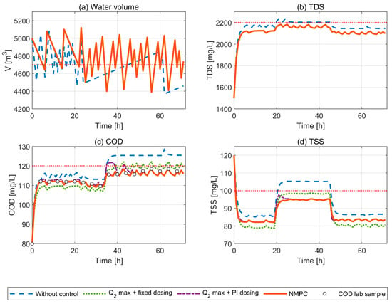
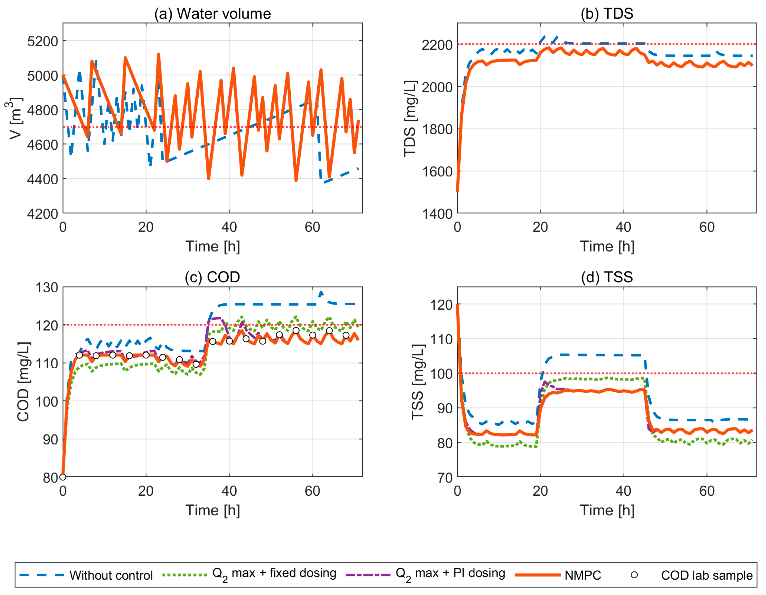
Under the simulated stress-test scenario S4, no control and fixed dosing violate all three limits for 24–37 h. Maximum dilution with fixed dosing removes the TDS and TSS violations but leaves 13 h of COD violations. With online measurements, both feedback strategies keep TDSs and TSSs within the limits; the PI controller incurs 1 h of COD violation (exceedance 0.3 mg·h/L) and NMPC none, with similar reagent consumption. When all indicators are measured online, a well-tuned PI controller therefore performs almost as well as NMPC for this process. Figure 3 shows the pond volume and water quality trajectories under scenario S4 with laboratory COD analyses every 4 h.

Figure 3. Pond volume (a) and water quality (b–d) under scenario S4 with COD laboratory analyses every 4 h (result delay 2 h); circles mark the COD samples. Red dotted lines—V_min and admissible limits. The curves for Q₂ max + fixed dosing, Q₂ max + PI dosing, and NMPC coincide in (a,b), since all three keep Q₂ at its maximum and reagents do not affect the volume or TDSs.

3.3. Control Actions

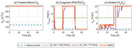
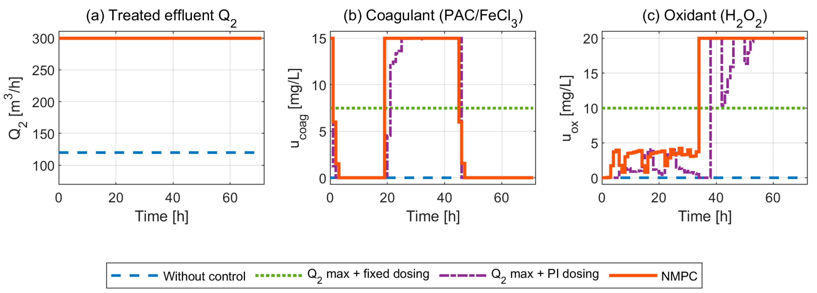
Figure 4 shows the control actions in scenario S4 with laboratory COD analyses every 4 h. NMPC keeps Q₂ at its upper bound throughout; TDSs are therefore governed by dilution alone and are identical for all strategies with a maximum Q₂. The coagulant dose is raised to its maximum at t = 20 h, when the ore change starts, and reduced after t = 45 h; the oxidant dose rises to 20 mg/L at t = 35 h, when CODs in the thickener overflow increase. Because the prediction holds disturbances at their current values, NMPC reacts only after a disturbance has begun; the reaction is immediate because the model-based estimate tracks CODs between analyses. The PI controller reacts to the COD increase only when a laboratory result reveals it and then needs several hours to reach the required dose (Figure 4c), which causes the COD violations in Figure 3c.

Figure 4. Control actions under scenario S4 with COD laboratory analyses every 4 h: treated-effluent flow Q₂ (a), coagulant dose (b), and oxidant dose (c).

3.4. Quantitative Comparison

Table 6 summarizes the performance metrics. Because the controller does not track concentration set-points, root-mean-square error (RMSE), with respect to set-points, is not reported. Instead, the number of hours with C > C_max (violations), the time-integrated exceedance above the limit, the minimum margin to the limit, and the mean reagent doses are used. Violations are counted for t > 0, i.e., excluding the initial state.

3.5. Laboratory-Based COD Measurement

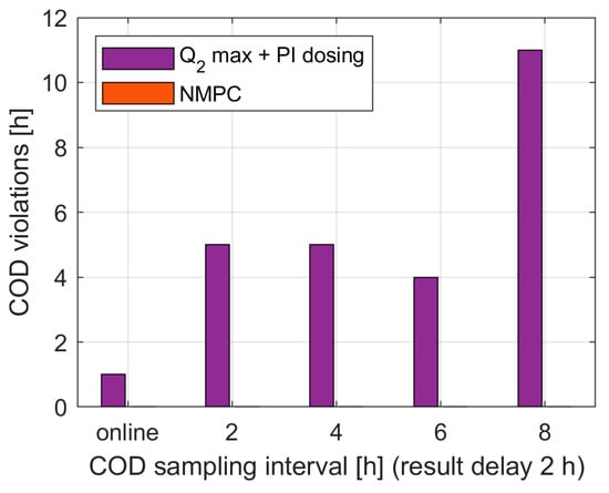
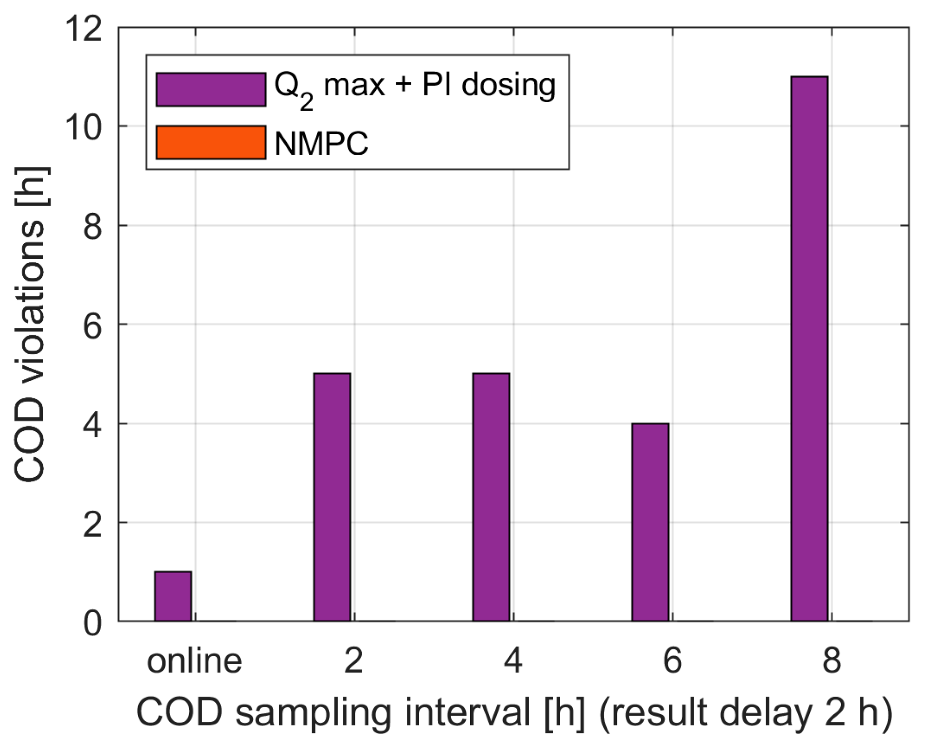
Table 7 and Figure 5 compare the PI controller and NMPC in scenario S4 when CODs are available only from laboratory analyses. The PI controller acts on outdated COD values and incurs 4–11 h of COD violations, the largest number at an 8 h sampling interval. NMPC, which estimates the current CODs with the model between analyses, incurs no COD violations at any sampling interval considered. The price is a higher oxidant consumption: 11.9 mg/L for NMPC against 8.1–10.9 mg/L for the PI controller (9–47% more), because NMPC acts on the predicted rather than on the last measured CODs. Coagulant consumption is similar (5.8 vs. 5.4 mg/L), since TSSs are measured online. Because the PI controller uses the last laboratory value (sample-and-hold), whereas NMPC uses a model-based COD estimate between analyses, this comparison reflects the combined benefit of the model-based state estimation and predictive optimization. The two contributions were not separated; this would require, for example, a PI controller acting on the same model-based estimate.

Table 7. COD violations and reagent use versus COD sampling interval (scenario S4, result delay 2 h).

COD Sampling	Q2 Max + PI: Violations TDSs/CODs/TSSs, h	Q2 Max + PI: ucoag/uox, mg/L	NMPC: Violations TDSs/CODs/TSSs, h	NMPC: ucoag/uox, mg/L
Online (hourly)	0/1/0	5.38/10.93	0/0/0	5.83/11.90
Every 2 h	0/5/0	5.38/9.96	0/0/0	5.83/11.90
Every 4 h	0/5/0	5.38/9.63	0/0/0	5.83/11.91
Every 6 h	0/4/0	5.38/10.04	0/0/0	5.83/11.91
Every 8 h	0/11/0	5.38/8.07	0/0/0	5.83/11.90

Figure 5. Hours of COD violation under scenario S4 versus the COD laboratory sampling interval (result delay 2 h) for the PI benchmark and NMPC; ‘online’ denotes hourly measurements without delay.

3.6. Plant–Model Mismatch

To test robustness, the simulated plant was given adversely perturbed parameters (kinetic coefficients reduced, internal sources increased), while the controller (prediction model and estimator) kept the nominal values (Table 8; scenario S4, COD analyses every 4 h). NMPC incurred no COD violations when k_coag, k_COD, or k_s were reduced by 30% and 3 h when the oxidation coefficient k_ox was 30% lower than assumed, against 5–8 h for the PI controller. With a combined adverse perturbation (all kinetic coefficients −20%, sources +20%), both controllers violated the COD limit, NMPC for 5 h and the PI controller for 10 h. A 30% increase in the internal sources caused 4 h of TDS violations for both, because TDSs can be reduced only by dilution and Q₂ was already at its maximum. The advantage of NMPC therefore persists under adverse parametric errors of up to 30% but is limited by the effectiveness of the oxidant, the least certain parameter of the model. Favorable perturbations (kinetic coefficients increased or sources reduced) were not tested.

Table 8. Plant–model mismatch (scenario S4, COD analyses every 4 h; controller model nominal).

Simulated Plant	Q2 Max + PI: Violations TDSs/CODs/TSSs, h	Q2 Max + PI: ucoag/uox, mg/L	NMPC: Violations TDSs/CODs/TSSs, h	NMPC: ucoag/uox, mg/L
Nominal	0/5/0	5.38/9.63	0/0/0	5.83/11.91
kox × 0.7	0/8/0	5.38/10.19	0/3/0	5.83/11.91
kcoag × 0.7	0/5/0	5.51/9.63	0/0/0	5.83/11.91
kCOD × 0.7	0/6/0	5.38/10.26	0/0/0	5.83/11.91
ks × 0.7	0/5/0	5.51/9.63	0/0/0	5.83/11.91
GTDS, GCOD, GTSS × 1.3	4/6/0	5.48/10.64	4/0/0	5.83/11.91
All k ×0.8, all G × 1.2	0/10/0	5.56/11.05	0/5/0	5.83/11.92

3.7. Weight Sensitivity and Solver Statistics

Table 9 shows that tenfold variations in the selected NMPC tuning weights (alarm-level, reagent-cost, move, and treated-effluent weights; Table 9) did not produce any violation in scenario S4 with laboratory COD analyses every 4 h. The minimum margins were unchanged (16.9, 1.5, and 4.7 mg/L for TDSs, CODs, and TSSs); only the reagent consumption changed (coagulant 5.6–6.8 mg/L, oxidant 11.2–12.9 mg/L). The conclusions are therefore not an artefact of these tuning weights; the hard-limit and volume penalty weights, which act as soft constraints, were not varied. In the same case, the SQP solver converged (exit flag > 0) at all 71 steps at the first attempt, without restarts, with on average 96 function evaluations per step (maximum 432) and an average computation time of 0.034 s per step (maximum 0.117 s) on a desktop computer. The computation time is reported as implementation information; real-time deployment was not assessed.

Table 9. NMPC weight sensitivity (scenario S4, COD analyses every 4 h).

Weights	Violations TDSs/CODs/TSSs, h	ucoag/uox, mg/L	Min. Margin TDSs/CODs/TSSs, mg/L
Nominal	0/0/0	5.83/11.91	16.9/1.5/4.7
wsoft × 0.1	0/0/0	5.70/11.40	16.9/1.5/4.7
wsoft × 10	0/0/0	5.83/12.08	16.9/1.5/4.7
wcoag, wox × 0.1	0/0/0	6.76/12.92	16.9/1.5/4.7
wcoag, wox × 10	0/0/0	5.63/11.23	16.9/1.5/4.7
wΔu × 0.1	0/0/0	5.63/11.39	16.9/1.5/4.7
wΔu × 10	0/0/0	6.61/12.70	16.9/1.5/4.7
wQ2 × 0.1	0/0/0	5.83/11.91	16.9/1.5/4.7
wQ2 × 10	0/0/0	5.83/11.91	16.9/1.5/4.7

4. Discussion

4.1. Interpretation of Results

The hypothesis that including TDSs, CODs, and TSSs in the NMPC state vector reduces violations of the process limits was confirmed relative to no control and fixed dosing, but the comparison with a PI feedback benchmark qualifies it. With the hourly online measurement of all indicators, a well-tuned PI controller with maximum dilution performed almost as well as NMPC (1 h vs. 0 h of COD violations in the simulated stress-test scenario S4). This follows from the process structure: the pond is hydraulically fast (residence time ≈ 1.2 h), and each reagent acts essentially on one indicator, so decoupled feedback loops are sufficient when measurements are timely.

The benefit of NMPC appears when CODs are measured only in the laboratory, which is the usual situation in concentrators [16]. The model-based estimate between analyses allowed NMPC to avoid COD violations at sampling intervals of up to 8 h, whereas the PI controller incurred 4–11 h of violations. This benefit is the combined effect of model-based COD estimations and predictive optimization: the PI benchmark acted on sample-and-hold laboratory values, and a PI controller supplied with the same model-based estimate was not tested, so the share attributable to prediction alone cannot be quantified. The benefit was retained under up to 30% adverse parametric mismatch and was insensitive to tenfold variations in the selected tuning weights, but it was obtained at the cost of 9–47% more oxidant; NMPC did not reduce reagent consumption relative to the PI benchmark.

TDSs are governed solely by hydraulic dilution: the reagents do not enter the TDS balance, and every strategy with Q₂ at its maximum produced the same TDS trajectory. The TDS improvement relative to no control is therefore a hydraulic effect, not a result of predictive optimization. Because the dominant inflow Q₁ carries TDSs close to the limit, dilution can keep TDSs below 2200 mg/L only while TDSs in the thickener overflow remain below about 2260 mg/L (for Q₂ = 300 m³/h and G_TDS ×1.35). Larger increases can be counteracted only by treatment that removes dissolved salts, for example lime–soda softening of the thickener overflow, which is outside the scope of the present model.

COD control is limited by the oxidant capacity: in scenario S4, NMPC kept the oxidant at its upper bound of 20 mg/L from t = 35 h, and the minimum COD margin was only 1.5 mg/L, so a stronger organic load would cause violations for any strategy. This confirms the dominant role of the reagent regime as an organic load source and argues for the joint optimization of reagent and water regimes [7,10].

4.2. Comparison with Existing Approaches

Unlike Noome (2023) [18] and Quintanilla et al. (2023–2024) [19], who address flotation cell control, to the best of the authors’ knowledge, this study is among the first to formulate NMPC at the closed-loop water circuit level with TDSs, CODs, and TSSs explicitly in the state vector. The closest analogues are Bernardelli et al. (2020) [31] and Aydin et al. (2019, 2022) [34,35]. Related MPC formulations have also been applied to reservoir flood control [36] and to anaerobic digestion [37].

4.3. Study Limitations

The study is simulation-based. The kinetic parameters k_COD, k_s, k_ox, and k_coag, the internal sources G_i, and the inlet concentrations were adopted from literature and design data without identification based on Aktogai operating data; k_ox and k_coag are of the order reported for related systems [29,30] and are the least certain parameters. The pseudo-first-order kinetics neglect the effects of the pH, temperature, and particle size distribution. The mismatch analysis covers adverse parametric errors of up to 30% but not favorable deviations or structural model errors, and the disturbance amplitudes of the stress scenario S4 were chosen for testing rather than derived from Aktogai operational data. The COD estimator is an open-loop model propagation between laboratory analyses; online TDS and TSS measurements are assumed to be available without delay or noise, and the design of a state observer with measurement noise and delays for all indicators remains future work. The flow rates were taken from the design documentation of a sister KAZ Minerals concentrator [15] and require verification against Aktogai SCADA data. The Q₄ safeguard is modeled as a simple hysteresis switch; its asymmetric treatment in the prediction (switch-off but no switch-on; Section 2.3.2) is a simplifying assumption that makes the prediction conservative whenever the safeguard is active, and the flows are constant apart from the scheduled change in Q₇. A promising direction is replacing the deterministic model with a data-driven approach based on Gaussian processes, as demonstrated for flotation control under partial observability [38].

4.4. Practical Significance

The study provides a simulation-based proof of concept. Its practical message for the Aktogai process water pond is that (i) TDSs can be managed only through hydraulic dilution, so the available treated effluent should be used at its maximum; (ii) when CODs and TSSs are measured online, simple PI dosing loops can be sufficient; and (iii) when CODs are available only from laboratory analyses, the combination of a model-based COD estimate and predictive control maintained the COD limit in the simulated stress test, where PI feedback based on delayed analyses did not. The economic benefit, which depends on reagent prices and on the effect of water quality on copper recovery, requires a separate techno-economic assessment. The TDS improvement relative to current operation results from the maximum use of treated effluent rather than from NMPC and part of the COD benefit may be obtainable by adding a model-based estimator to conventional feedback loops.

5. Conclusions

This work developed a nonlinear dynamic model of the closed-loop process water circuit of the Aktogai GOK flotation plant with nine process flows and the state vector:

$$x={\left[\begin{array}{cccc}V& \mathit{TDS}& \mathit{COD}& \mathit{TSS}\end{array}\right]}^T.$$

The model includes pseudo-first-order kinetics for COD oxidation (H₂O₂, k_ox = 0.003 L/(mg·h)) and TSS coagulation (PAC/FeCl₃, k_coag = 0.005 L/(mg·h)). An NMPC problem was formulated with three manipulated variables, u = [Q₂, u_coag, u_ox], an 8 h prediction horizon with two move blocks, normalized one-sided soft constraints, and a reagent cost, and was solved by SQP. The internal recirculation Q₅ was shown to have no net effect on the pond and was excluded from the balances.

Simulations over 72 h showed the following: (1) under nominal disturbances, all strategies met the limits, and maximum dilution increased the TDS margin from 3 to 60 mg/L; (2) under the simulated stress-test scenario, NMPC and a well-tuned PI controller with maximum dilution both met the TDS and TSS limits, and with online measurements, they performed almost equally (0 vs. 1 h of COD violation); (3) with laboratory COD analyses every 2–8 h, NMPC avoided COD violations completely, whereas the PI controller incurred 4–11 h, at the cost of 9–47% more oxidant, a benefit that reflects the model-based COD estimation combined with predictive optimization; (4) the advantage of NMPC persisted under up to 30% adverse parametric mismatch and was insensitive to tenfold variations in the selected tuning weights; and (5) TDS can be kept below the limit only through dilution, independently of the control strategy, and only while the thickener-overflow TDSs remain below about 2260 mg/L.

Future research should focus on the following: (1) identification of k_COD, k_s, k_ox, k_coag, and G_i from Aktogai laboratory information management system (LIMS) and SCADA data; (2) separating the contributions of model-based estimation and predictive optimization, e.g., with a PI controller acting on the same COD estimate, and the design of a state observer accounting for measurement noise and delays; (3) inclusion of salt-removing treatment, such as lime–soda softening, as an additional manipulated variable for TDSs and hardness; and (4) a techno-economic assessment of the reagent consumption and copper recovery.

References

- Karkou, E.; Teo, C.J.; Savvakis, N.; Poinapen, J.; Arampatzis, G. Industrial circular water use practices through the application of a conceptual water efficiency framework in the process industry. J. Environ. Manag. 2024, 370, 122596. [Google Scholar] [CrossRef] [Scilit] [PubMed]
- OECD. The Economics of Water Scarcity; OECD Publishing: Paris, France, 2024. [Google Scholar] [CrossRef] [Scilit]
- Atakhanova, Z.; Meirambayeva, M.; Baigaliyeva, M. Mine Water Use in Kazakhstan: Data Issues, Risks, and Regulations. Sustainability 2024, 16, 2456. [Google Scholar] [CrossRef] [Scilit]
- Meissner, S. The Impact of Metal Mining on Global Water Stress and Regional Carrying Capacities. Resources 2021, 10, 120. [Google Scholar] [CrossRef] [Scilit]
- Irandoost, E.; Ghorbanpour, A.; Balouei Jamkhaneh, H.; Ghasemi, P.; Babaee Tirkolaee, E. Sustainable-circular water resources management in the mining industry using system dynamics modeling. Water Resour. Ind. 2025, 34, 100313. [Google Scholar] [CrossRef] [Scilit]
- KAZ Minerals. Sustainability Report 2021; KAZ Minerals Limited: London, UK, 2022; Available online: www.kazminerals.com (accessed on 15 October 2026).
- Evdokimov, S.I. Flotation Beneficiation Methods: Teaching Manual; SKGMI (GTU): Vladikavkaz, Russia, 2021. (In Russian) [Google Scholar]
- Atakhanova, Z.; Azhibay, S. Assessing Economic Sustainability of Mining in Kazakhstan. Miner. Econ. 2023, 36, 719–731. [Google Scholar] [CrossRef] [Scilit]
- Li, C.; Shen, P.; Pan, H.; Cao, C.; Seitmuratova, E. Geology and ore-forming fluid evolution of the Aktogai giant porphyry Cu deposit, Kazakhstan. J. Asian Earth Sci. 2018, 165, 192–209. [Google Scholar] [CrossRef] [Scilit]
- Soufiabadi, A.M.; Nejadaria, M.; Dehghan, R.; Safari, M.; Hassanzadeh, A.; Khoshdast, H. Effect of different process water sources on rougher flotation efficiency of a copper ore: A case study at Sarcheshmeh Copper Complex. Physicochem. Probl. Miner. Process. 2023, 59, 184087. [Google Scholar] [CrossRef] [Scilit]
- Manono, M.S.; Corin, K.C.; Wiese, J.G. The effect of ionic strength of plant water on frother behaviour. Miner. Eng. 2020, 158, 106593. [Google Scholar]
- Bicak, O.; Ekmekci, Z.; Ozturk, Y. The effect of water chemistry on froth stability and surface chemistry of flotation of a Cu–Zn sulfide ore. Int. J. Miner. Process. 2012, 102–103, 32–37. [Google Scholar] [CrossRef] [Scilit]
- Wills, B.A.; Finch, J. Wills’ Mineral Processing Technology, 9th ed.; Elsevier: Amsterdam, The Netherlands, 2023. [Google Scholar]
- Corin, K.C.; Reddy, A.; Miyen, L.; Wiese, J.G.; Harris, P.J. The effect of ionic strength of plant water on valuable mineral and gangue recovery in a platinum bearing ore from the Merensky reef. Miner. Eng. 2011, 24, 131–137. [Google Scholar] [CrossRef] [Scilit]
- KAZ Minerals Bozshakol LLP. Description of the Process and Potable Water Supply Process; Internal Technical Document; KAZ Minerals Bozshakol LLP: Ekibastuz, Kazakhstan, 2015. (In Russian) [Google Scholar]
- Le, T.M.K.; Miettinen, H.; Bomberg, M.; Schreithofer, N.; Dahl, O. Challenges in the assessment of mining process water quality. Minerals 2020, 10, 940. [Google Scholar] [CrossRef] [Scilit]
- Levay, G.; Schumann, R. A systematic approach to water quality management in the minerals processing industry. In Proceedings of the Water in Mining Conference, Brisbane, Australia, 14–16 November 2006; pp. 1–10. [Google Scholar]
- Noome, Z.M. Nonlinear model predictive control for mineral processing systems under process disturbances. J. Process Control 2023, 129, 103067. [Google Scholar]
- Quintanilla, P.; Valencia, F.; Cipriano, A. Experimental implementation of economic nonlinear model predictive control for flotation processes. IFAC-PapersOnLine 2024, 58, 245–250. [Google Scholar]
- Quintanilla, P.; Navia, D.; Neethling, S.J.; Brito-Parada, P.R. Centralised economic model predictive control of froth flotation banks. Chem. Eng. Res. Des. 2025, 224, 467–481. [Google Scholar] [CrossRef] [Scilit]
- Shean, B.J.; Cilliers, J.J. A review of froth flotation control. Int. J. Miner. Process. 2011, 100, 57–71. [Google Scholar] [CrossRef] [Scilit]
- Hodouin, D. Methods for automatic control, observation, and optimization in mineral processing plants. J. Process Control 2011, 21, 211–225. [Google Scholar] [CrossRef] [Scilit]
- Markabayeva, Z.; Koshimbayev, K.; Abzhanova, L.; Orakbaev, Y.; Sagyndykova, S. Analysis of modern methods for control and management of the flotation process. News Natl. Acad. Sci. Repub. Kazakhstan Ser. Geol. Technol. Sci. 2025, 3, 109–119. [Google Scholar] [CrossRef] [Scilit]
- Department of Ecology of Abai Region. Conclusion on the Scope of EIA for KAZ Minerals Aktogay LLP, Kyzylkiya Site; No. KZ51VWF00095949; Department of Ecology of Abai Region: Semey, Kazakhstan, 2023. (In Russian) [Google Scholar]
- KAZ Minerals. Aktogai Sulphide Concentrator Expansion Project; Environmental Impact Assessment; KAZ Minerals: Almaty, Kazakhstan, 2018. [Google Scholar]
- KAZ Minerals PLC. Aktogay Expansion Project Approved; Announcement; KAZ Minerals PLC: London, UK, 21 December 2017; Available online: https://www1.hkexnews.hk/listedco/listconews/sehk/2017/1221/ltn20171221763.pdf (accessed on 15 October 2026).
- Rao, S.R.; Finch, J.A. A review of water re-use in flotation. Miner. Eng. 1989, 2, 65–86. [Google Scholar] [CrossRef] [Scilit]
- Levay, G.; Smart, R.S.C.; Skinner, W.M. The impact of water quality on flotation performance. J. S. Afr. Inst. Min. Metall. 2001, 101, 69–75. [Google Scholar]
- Deng, Y.; Englehardt, J.D. Treatment of landfill leachate by the Fenton process. Water Res. 2006, 40, 3683–3694. [Google Scholar] [CrossRef] [Scilit] [PubMed]
- Duan, J.; Gregory, J. Coagulation by hydrolysing metal salts. Adv. Colloid. Interface Sci. 2003, 100–102, 475–502. [Google Scholar] [CrossRef] [Scilit]
- Bernardelli, A.; Marsili-Libelli, S.; Manzini, A.; Stancari, S.; Tardini, G.; Montanari, D.; Anceschi, G.; Gelli, P.; Venier, S. Real-time model predictive control of a wastewater treatment plant based on machine learning. Water Sci. Technol. 2020, 81, 2391–2400. [Google Scholar] [CrossRef] [Scilit] [PubMed]
- Flores-Alsina, X.; Corominas, L.; Snip, L.; Vanrolleghem, P.A. Including greenhouse gas emissions during benchmarking of wastewater treatment plant control strategies. Water Res. 2011, 45, 4700–4710. [Google Scholar] [CrossRef] [Scilit] [PubMed]
- Rawlings, J.B.; Mayne, D.Q.; Diehl, M. Model Predictive Control: Theory and Design; Nob Hill Publishing: Santa Barbara, CA, USA, 2017. [Google Scholar]
- Aydin, B.E.; Delsman, J.; van de Giesen, N.; Abraham, E. Nonlinear model predictive control of salinity and water level in polder networks: Case study of Lissertocht catchment. Agric. Water Manag. 2022, 264, 107502. [Google Scholar] [CrossRef] [Scilit]
- Aydin, B.; Tian, X.; Delsman, J.; Oude Essink, G.H.P.; Rutten, M.; Abraham, E. Optimal salinity and water level control of water courses using Model Predictive Control. Environ. Model. Softw. 2019, 112, 36–45. [Google Scholar] [CrossRef] [Scilit]
- Koo, J.-H.; Abraham, E.; Jonoski, A.; Solomatine, D.P. Balancing operator’s risk averseness in model predictive control for real-time reservoir flood control. J. Hydroinformatics 2025, 27, 601–624. [Google Scholar] [CrossRef] [Scilit]
- Moradvandi, A.; De Schutter, B.; Abraham, E.; Lindeboom, R.E. Model predictive control of feed rate for stabilizing and enhancing biogas production in anaerobic digestion under meteorological fluctuations. J. Process Control 2025, 147, 103375. [Google Scholar] [CrossRef] [Scilit]
- Wang, Y.; del Río Chanona, E.A.; Quintanilla, P. Gaussian process nonlinear model predictive control for online partially observable systems: An application to froth flotation. Ind. Eng. Chem. Res. 2025, 64, 13307–13322. [Google Scholar] [CrossRef] [Scilit]
Disclaimer/Publisher’s Note: The statements, opinions and data contained in all publications are solely those of the individual author(s) and contributor(s) and not of MDPI and/or the editor(s). MDPI and/or the editor(s) disclaim responsibility for any injury to people or property resulting from any ideas, methods, instructions or products referred to in the content. |
© 2026 by the authors. Licensee MDPI, Basel, Switzerland. This article is an open access article distributed under the terms and conditions of the Creative Commons Attribution (CC BY) license.