CFD Analysis of Coronary Artery Blood Flow Using an Ad Hoc OpenFOAM CFD Solver

Abstract

Coronary blood flow is governed by the interaction between pulsatile aortic haemodynamics, the downstream vascular response, and the time-dependent compression exerted by the myocardium. This study presents a custom OpenFOAM solver for simulation of aortic–coronary haemodynamics. The numerical framework combines a power-law inlet velocity profile selected according to the estimated Womersley regime, a three-element Windkessel condition at the aortic outlet, and dedicated lumped-parameter boundary conditions at the coronary outlets, including the effect of intramyocardial pressure. The methodology was applied to two patient-specific aortic–coronary geometries reconstructed from computed tomography data. Numerical discretisation uncertainty was assessed using three mesh resolutions, while the spatial resolution of the detached-eddy simulation was examined by comparing modelled and resolved kinetic-energy contributions. The methodology developed reproduced pulsatile velocity and pressure fields, geometry-dependent recirculation patterns, and distinct pressure responses along the aortic and coronary pathways. Computed velocity and pressure magnitudes were of the same physiological scale as available in vivo coronary measurements. The proposed framework provides a computational methodology for investigating local haemodynamics in patient-specific aortic–coronary anatomies while accounting for the downstream coronary circulation and intramyocardial effects.

1. Introduction

The right and left coronary arteries supply blood to the myocardium and constitute the coronary circulation, which receives approximately 5% of the cardiac output. They originate from the ascending aorta at the level of the aortic sinuses. The left coronary artery bifurcates into the circumflex artery, which gives rise to the marginal branches, and the left anterior descending artery, which gives rise to diagonal and septal branches. The right coronary artery runs between the right atrium and ventricle and extends towards the inferior portion of the interventricular septum [1,2].

Coronary artery disease remains one of the leading causes of morbidity and mortality worldwide, highlighting the importance of prevention, diagnosis, and haemodynamic assessment. Atherosclerosis, namely the development of plaques within the arterial wall, is commonly associated with lipid deposition and inflammatory processes [3]. Regions of bifurcation, curvature, and stenosis are particularly relevant because they are often characterised by disturbed or non-uniform blood flow, which may affect endothelial function and plaque development [4]. Therefore, the quantitative description of local haemodynamics is essential for understanding the relationship between vascular morphology, flow patterns, and coronary pathology [5].

Diagnostic assessment of cardiovascular disease relies on several imaging techniques, including cardiac magnetic resonance imaging, stress echocardiography, single-photon emission computed tomography, positron emission tomography, computed tomography angiography, and invasive coronary angiography [6]. Cardiac magnetic resonance imaging can provide information on vascular stiffness and aortic pulse-wave velocity, which are associated with left ventricular dysfunction, aneurysm formation, atherosclerosis, myocardial infarction, and stroke [7]. Advanced four-dimensional flow imaging can also estimate velocity fields and pressure distributions in large vessels [8]. However, the direct assessment of detailed coronary flow remains challenging because of the small vessel calibre, complex curvature, cardiac motion, and limited spatial and temporal resolution of clinical imaging techniques [9]. As a result, quantities such as wall shear stress, pressure drop, flow separation, and branch flow partition are difficult to measure directly with sufficient detail.

Computational fluid dynamics (CFD) has emerged as a complementary methodology for studying cardiovascular flows, since it enables the reconstruction of local haemodynamic fields that cannot be directly measured with standard diagnostic techniques [10]. By combining patient-specific vascular geometries, physiological boundary conditions, and numerical solution of the governing equations, CFD allows the estimation of velocity, pressure, wall shear stress, and other derived indicators relevant to vascular disease [11]. Its role has been demonstrated in several vascular districts. For example, patient-specific CFD models of cerebral aneurysms can reconstruct local flow patterns and haemodynamic quantities potentially related to aneurysm evolution and rupture risk [12]. Similarly, CFD studies of the vertebrobasilar junction can provide information on shear stress, particle trajectories, coherent flow structures, and mixing phenomena between the vertebral arteries [13]. Advanced imaging techniques, such as 7D-MRV and phase-contrast magnetic resonance imaging, can directly measure velocity fields in selected vascular regions, but their accuracy may be affected by resolution limits and artefacts in complex-flow regions; CFD can therefore complement these measurements by providing more detailed velocity and shear-related fields [14].

In coronary arteries, CFD modelling presents additional challenges. Coronary flow is intrinsically pulsatile and strongly influenced by the interaction between the heart and the vascular system [3]. During ventricular contraction, intramyocardial pressure rises and can reduce coronary perfusion, whereas ventricular relaxation decreases the compressive action and promotes diastolic flow. Consequently, coronary blood flow cannot be realistically described by generic outlet boundary conditions alone, because the distal vascular bed and the myocardium introduce a time-dependent impedance that affects both pressure and flow waveforms.

The inlet boundary condition also plays an important role in reproducing physiological coronary haemodynamics. In many cardiovascular CFD studies, simplified plug or parabolic profiles are imposed at the inlet. However, pulsatile arterial flow depends on the balance between unsteady inertial and viscous effects, commonly described through the Womersley number. At low Womersley numbers, viscous effects dominate and the velocity profile tends to remain parabolic, whereas at higher Womersley numbers the profile becomes flatter in the vessel core. In the present work, the inlet condition is therefore based on a power-law velocity profile scaled according to the Womersley number.

The prescription of outlet boundary conditions is equally critical. In a previous work by the authors, an OpenFOAM-based methodology was developed for patient-specific aortic blood-flow simulations, including a Windkessel pressure boundary condition for arterial outflows [11]. Although this model provides a physiological pressure–flow coupling for non-coronary outlets, coronary branches require a dedicated formulation because the downstream coronary circulation is affected by myocardial compression. A specific lumped-parameter model is therefore needed to account for the interaction between coronary vessels, microcirculation, and intramyocardial pressure [3].

OpenFOAM is particularly suitable for this development because of its open-source structure, finite-volume formulation, and high degree of customisability. Its C++ architecture allows the implementation of dedicated solvers and boundary conditions for cardiovascular applications, while retaining robust numerical algorithms, support for unstructured meshes, and standard post-processing tools [11].

The aim of the present work is to assess a custom OpenFOAM solver for coronary blood-flow simulation. The solver extends the authors’ previous cardiovascular CFD framework by incorporating: (i) a dedicated coronary outlet boundary condition based on a lumped-parameter model including intramyocardial effects; (ii) an inlet velocity boundary condition based on a Womersley-power-law profile; and (iii) the Windkessel pressure boundary condition previously developed for arterial outflows [11]. The methodology is applied to patient-specific coronary geometries to evaluate the ability of the solver to reproduce physiologically consistent pressure and velocity fields and to provide haemodynamic quantities relevant to coronary-flow analysis.

In perspective, the proposed framework may support the analysis of healthy and pathological coronary configurations, enabling the evaluation of local haemodynamic indicators such as pressure distribution, velocity patterns, wall shear stress, and branch flow partition. Once validated against experimental or clinical reference data, the solver may also provide a basis for reduced-order modelling and data-driven acceleration strategies, including Physics-Informed Neural Networks, aimed at reducing the computational cost of patient-specific cardiovascular simulations [15].

2. Mathematical and Numerical Method

2.1. Governing Equations

The blood flow in the coronary arteries was modelled as an incompressible, unsteady flow governed by the conservation of mass and momentum. The incompressibility assumption is justified by the nearly constant density of blood under physiological conditions and by the relatively low flow velocities involved in cardiovascular applications [16,17]. The governing equations are therefore the incompressible continuity equation and the Navier–Stokes momentum equation:

$$\nabla ·\mathbf{u}=0,$$

(1)

$${\displaystyle \frac{\partial \mathbf{u}}{\partial t}}+\mathbf{u}·\nabla \mathbf{u}=-{\displaystyle \frac{\nabla p}{\rho }}+\mathbf{f}+\nu {\nabla }^2\mathbf{u},$$

(2)

where $\mathbf{u}$ is the velocity vector, p is the pressure, $\rho$ is the blood density, $\nu$ is the kinematic viscosity, and $\mathbf{f}$ represents possible body-force contributions.

The resulting system consists of four coupled partial differential equations: one equation for mass conservation and three equations for momentum conservation. An implicit pressure–velocity coupling procedure with a projection-like predictor–corrector structure was adopted for the numerical solution. The momentum predictor was followed by a pressure-correction equation enforcing mass conservation and correcting the velocity field. In OpenFOAM, this coupling was handled through the PIMPLE algorithm [11,18,19,20].

Although blood is a non-Newtonian fluid because of its cellular composition and the interactions among its suspended components, it is commonly approximated as a Newtonian fluid in cardiovascular CFD simulations when the characteristic shear rates are sufficiently high [21,22,23]. This approximation was adopted throughout the computational domain, consistently with previous numerical studies of coronary blood flow [24,25]. Blood was therefore characterised by a constant density $\rho =1060\mathrm{kg}{\mathrm{m}}^{-3}$ and a constant kinematic viscosity $\nu =4.0\times {10}^{-6}{\mathrm{m}}^2{\mathrm{s}}^{-1}$, corresponding to a dynamic viscosity $\mu =\rho \nu =4.2\times {10}^{-3}\mathrm{Pa}\mathrm{s}$. The adopted values are consistent with those commonly used in cardiovascular CFD simulations [26,27,28].

Because coronary flow is highly sensitive to the imposed haemodynamic forcing, the prescription of physiologically consistent boundary conditions is essential for obtaining meaningful numerical results. For this reason, the following subsections are devoted to the boundary-condition framework implemented in the solver. The aortic inlet condition is first presented, in which the measured flow-rate waveform is imposed through a Womersley-based power-law velocity profile [29]. The outlet conditions are then described, with particular attention to the reduced-order pressure models adopted to represent the downstream vascular response: the Windkessel model for the aortic outlet and the coronary lumped-parameter model for the coronary branches.

2.2. Aortic Inlet

At the aortic inlet, a time-dependent velocity boundary condition was prescribed starting from a measured volumetric flow-rate waveform. The waveform was provided as a discrete table of pairs $\left(t,Q\left(t\right)\right)$ and stored in the file constant/inletFlowRate.foam. During the simulation, the instantaneous value of the inlet flow rate was obtained by linear interpolation of the tabulated data.

The inlet velocity distribution was not imposed as a spatially uniform profile. Instead, a power-law profile was adopted in order to account for the blunted shape typically associated with pulsatile flow in large arteries. The normal velocity over the inlet section was prescribed as

$$u_n(r,t)=U_{\max }\left(t\right)\left[1-{\left({\displaystyle \frac{r}{R_{\mathrm{eff}}}}\right)}^n\right],$$

(3)

where r is the radial distance from the inlet-section centroid, $R_{\mathrm{eff}}$ is the effective inlet radius, n is the power-law exponent, and $U_{\max }\left(t\right)$ is the maximum velocity at the centre of the inlet section. The velocity vector was then imposed along the inward normal direction to the inlet patch:

$$\mathbf{u}(\mathbf{x},t)=u_n(r,t){\mathbf{n}}_{\mathrm{in}},$$

(4)

where ${\mathbf{n}}_{\mathrm{in}}$ denotes the inward-pointing unit normal vector.

The effective inlet radius was computed from the inlet-patch area as

$$R_{\mathrm{eff}}=\sqrt{{\displaystyle \frac{A_{\mathrm{in}}}{\pi }}},$$

(5)

with

$$A_{\mathrm{in}}={\int }_{{\mathsf{\Gamma }}_{\mathrm{in}}}d\mathsf{\Gamma }.$$

(6)

The centroid of the inlet section was evaluated using an area-weighted average of the face centres. This allowed the local radial coordinate r to be computed directly on the actual inlet patch.

The value of $U_{\max }\left(t\right)$ was determined by enforcing consistency between the imposed velocity profile and the prescribed volumetric flow rate. Hence, the following constraint was imposed:

$$Q\left(t\right)={\int }_{{\mathsf{\Gamma }}_{\mathrm{in}}}\mathbf{u}(\mathbf{x},t)·{\mathbf{n}}_{\mathrm{in}}d\mathsf{\Gamma }.$$

(7)

Assuming the power-law profile of Equation (3) over an equivalent circular section, the integral gives

$$Q\left(t\right)=U_{\max }\left(t\right)A_{\mathrm{in}}{\displaystyle \frac{n}{n+2}}.$$

(8)

Therefore, the maximum velocity was computed as

$$U_{\max }\left(t\right)={\displaystyle \frac{n+2}{n}}{\displaystyle \frac{Q\left(t\right)}{A_{\mathrm{in}}}}.$$

(9)

This normalisation ensures that the surface integral of the imposed velocity field is consistent with the prescribed instantaneous flow rate.

The profile exponent n controls the shape of the inlet velocity distribution. For $n=2$, Equation (3) corresponds to a parabolic Poiseuille-like profile, for which $U_{\max }=2Q/A_{\mathrm{in}}$. Larger values of n produce progressively flatter profiles. The value of n can be selected according to the Womersley number associated with the aortic inlet, so that the imposed velocity profile could reproduce the expected transition from a quasi-parabolic profile at low Womersley numbers to a blunter distribution when unsteady inertial effects become dominant.

2.3. Aortic Outlet Windkessel Boundary Condition

The outlet boundary conditions were defined separately for the aortic and coronary districts. A three-element Windkessel model was applied at the aortic outlet, whereas a dedicated multi-parameter lumped model was adopted for the coronary outlets. Since the Windkessel pressure boundary condition was already developed and discussed in detail in a previous work by the authors [11], only its main formulation is briefly recalled here.

The three-element Windkessel model represents the downstream arterial system through an electrical analogue composed of a proximal resistance $R_p$, a distal resistance $R_d$, and a compliance C. The resistances account for the pressure losses associated with the downstream circulation, while the compliance represents the elastic storage capacity of the arterial system during the cardiac cycle. The corresponding pressure–flow relation is

$$\left(1+{\displaystyle \frac{R_d}{R_p}}\right)Q\left(t\right)+C{R}_d{\displaystyle \frac{dQ\left(t\right)}{dt}}={\displaystyle \frac{P\left(t\right)}{R_p}}+C{\displaystyle \frac{dP\left(t\right)}{dt}},$$

(10)

where $Q\left(t\right)$ is the outlet flow rate and $P\left(t\right)$ is the outlet pressure.

The model parameters were estimated from physiological quantities. The total systemic resistance was first computed as

$$R_{\mathrm{tot}}={\displaystyle \frac{P_{\mathrm{mean}}}{CO}},$$

(11)

where $P_{\mathrm{mean}}$ is the mean arterial pressure and $CO$ is the cardiac output. The proximal and distal resistances were then assigned as

$$\begin{array}{cc}\hfill R_d& =0.91R_{\mathrm{tot}},\hfill \\ \hfill R_p& =0.09R_{\mathrm{tot}}.\hfill \end{array}$$

(12)

following the usual separation between proximal and peripheral resistance contributions [30,31,32,33,34].

Finally, the compliance was estimated from the diastolic pressure decay through the Windkessel time constant,

$$\tau =R_{d}C=-{\displaystyle \frac{t_{\mathrm{dias}}}{\ln \left(P_{\mathrm{dias}}/P_0\right)}},$$

(13)

where $t_{\mathrm{dias}}$ is the diastolic time interval, $P_0$ is the pressure at the beginning of diastole, and $P_{\mathrm{dias}}$ is the diastolic pressure [35].

2.4. Coronary Outlet Boundary Condition

The coronary outlet sections were treated by means of a dedicated lumped-parameter model, aimed at reproducing the main features of coronary pressure and flow waveforms. Unlike the aortic outlet, where a three-element Windkessel model was adopted, the coronary outlets require a specific formulation because the distal coronary vascular bed is affected by the time-dependent compressive action exerted by the myocardium.

The model represents the coronary vascular bed through resistive and capacitive elements, together with the intramyocardial pressure. For each coronary outlet, the following quantities are introduced: the coronary arterial resistance $R_a$, the coronary arterial microcirculatory resistance $R_{a\text{-}micro}$, the coronary venous resistance $R_v$, the coronary venous microcirculatory resistance $R_{v\text{-}micro}$, the arterial compliance $C_a$, the intramyocardial compliance $C_{im}$, and the intramyocardial pressure $P_{im}\left(t\right)$.

Based on these quantities, the following coefficients are defined:

$$\begin{array}{cc}\hfill p_0& =1,\hfill \\ \hfill p_1& =R_{a\text{-}micro}{C}_a+\left(R_v+R_{v\text{-}micro}\right)\left(C_a+C_{im}\right),\hfill \\ \hfill p_2& =R_{a\text{-}micro}{C}_a{C}_{im}\left(R_v+R_{v\text{-}micro}\right),\hfill \\ \hfill q_0& =R_{a\text{-}micro}+R_a+R_v+R_{v\text{-}micro},\hfill \\ \hfill q_1& =R_a{C}_a\left(R_v+R_{v\text{-}micro}+R_{a\text{-}micro}\right)+C_{im}\left(R_a+R_{a\text{-}micro}\right)\left(R_v+R_{v\text{-}micro}\right),\hfill \\ \hfill q_2& =C_a{C}_{im}{R}_a{R}_{a\text{-}micro}\left(R_v+R_{v\text{-}micro}\right),\hfill \\ \hfill b_0& =0,\hfill \\ \hfill b_1& =C_{im}\left(R_v+R_{v\text{-}micro}\right).\hfill \end{array}$$

(14)

These coefficients combine the resistive and capacitive contributions of the coronary and myocardial compartments and are used to express the pressure response of the reduced-order model.

The auxiliary coefficients required for the analytical solution of the lumped model are

$$\begin{array}{cc}\hfill {\lambda }_{1,2}& ={\displaystyle \frac{-p_1\pm \sqrt{p_1^2-4p_0{p}_2}}{2p_2}},\hfill \\ \hfill R& ={\displaystyle \frac{q_2}{p_2}},\hfill \\ \hfill Z_{1,2}& ={\displaystyle \frac{q_2{\lambda }_{1,2}^2+q_1{\lambda }_{1,2}+q_0}{\sqrt{p_1^2-4p_0{p}_2}}},\hfill \\ \hfill Y_{1,2}& ={\displaystyle \frac{b_1{\lambda }_{1,2}+b_0}{\sqrt{p_1^2-4p_0{p}_2}}},\hfill \\ \hfill A& ={\displaystyle \frac{-1}{\sqrt{p_1^2-4p_0{p}_2}}}\left[(q_2{\lambda }_1+q_1)Q\left(0\right)+q_2{\displaystyle \frac{dQ}{dt}}\left(0\right)+b_1{P}_{im}\left(0\right)+p_2\left({\lambda }_{2}P\left(0\right)-{\displaystyle \frac{dP}{dt}}\left(0\right)\right)\right],\hfill \\ \hfill B& ={\displaystyle \frac{-1}{\sqrt{p_1^2-4p_0{p}_2}}}\left[(q_2{\lambda }_2+q_1)Q\left(0\right)+q_2{\displaystyle \frac{dQ}{dt}}\left(0\right)+b_1{P}_{im}\left(0\right)+p_2\left({\lambda }_{1}P\left(0\right)-{\displaystyle \frac{dP}{dt}}\left(0\right)\right)\right].\hfill \end{array}$$

(15)

where $Q\left(t\right)$ and $P\left(t\right)$ denote, respectively, the flow rate and pressure at the coronary outlet.

Following the formulation proposed by Mantero et al. [36], for each coronary outlet, the lumped-parameter model provides a scalar pressure response as a function of the instantaneous outlet flow rate, of the flow-rate history, and of the prescribed intramyocardial pressure. Defining the history integrals

$$\begin{array}{cccc}\hfill I_{Q,1}\left(t\right)& ={\int }_0^t{e}^{{\lambda }_1(t-s)}Q\left(s\right)ds,\hfill & \hfill I_{Q,2}\left(t\right)& ={\int }_0^t{e}^{{\lambda }_2(t-s)}Q\left(s\right)ds,\hfill \\ \hfill I_{P_{im},1}\left(t\right)& ={\int }_0^t{e}^{{\lambda }_1(t-s)}{P}_{im}\left(s\right)ds,\hfill & \hfill I_{P_{im},2}\left(t\right)& ={\int }_0^t{e}^{{\lambda }_2(t-s)}{P}_{im}\left(s\right)ds,\hfill \end{array}$$

(16)

the pressure returned by the coronary outlet model can be written as

$$\begin{array}{cc}\hfill P_{\mathrm{cor}}\left(t\right)& =RQ\left(t\right)+Z_1{I}_{Q,1}\left(t\right)-Z_2{I}_{Q,2}\left(t\right)+A{e}^{{\lambda }_{1}t}-B{e}^{{\lambda }_{2}t}\hfill \\ \hfill & +Y_1{I}_{P_{im},1}\left(t\right)-Y_2{I}_{P_{im},2}\left(t\right).\hfill \end{array}$$

(17)

In the OpenFOAM implementation, Equation (17) is evaluated independently for each coronary outlet. The instantaneous flow rate $Q\left(t\right)$ is obtained by integrating the surface flux over the corresponding outlet patch, while $P_{im}\left(t\right)$ is prescribed as a time-dependent waveform and interpolated at the current simulation time. The resulting scalar pressure is stored for the corresponding outlet and subsequently imposed uniformly on the pressure patch through the dedicated CBC boundary condition.

The history integrals in Equation (16) are advanced recursively. For a generic forcing term $X\left(t\right)$ associated with the exponential mode ${\lambda }_k$, the corresponding history contribution is updated as

$$I_k^n=I_k^{n-1}\exp \left({\lambda }_k\mathsf{\Delta }t\right)+X^n\mathsf{\Delta }t,$$

(18)

where $\mathsf{\Delta }t$ is the CFD time step. In the implementation, four history terms are stored for each coronary outlet: two associated with the outlet flow rate and two associated with the intramyocardial pressure. Equation (18) corresponds to a first-order (rectangle-rule) quadrature of the convolution integrals, consistent with the first-order temporal discretisation of the flow solver. Its relative error scales as $|{\lambda }_k|\mathsf{\Delta }t/2$; for the present parameters, $|{\lambda }_k|$ ranges from approximately $1.9$ to $11{\mathrm{s}}^{-1}$ (time constants between $0.09$ and $0.53\mathrm{s}$), so that, with the time steps used in the simulations ($\mathsf{\Delta }t\le 3.6\times {10}^{-5}$ s), the error introduced in the history integrals, and therefore in the outlet pressure, is below $0.03\%$. Similarly, the homogeneous terms $A{e}^{{\lambda }_{1}t}$ and $B{e}^{{\lambda }_{2}t}$ decay with the same time constants and are negligible after the ten simulated cardiac cycles. For each coronary outlet, the reduced-order model returns a scalar physical pressure value.

The outlet-specific coronary parameters are defined through the arterial resistance $R_a$, the venous resistance $R_v$, the arterial and venous microcirculatory resistances $R_{a\text{-}micro}$ and $R_{v\text{-}micro}$, the arterial compliance $C_a$, and the intramyocardial compliance $C_{im}$. Since the total coronary resistance is higher than the systemic vascular resistance, it was estimated as

$$R_{\mathrm{coronary}}=24R_{\mathrm{systemic}}.$$

(19)

According to Murray’s law, this total coronary resistance was distributed among the coronary outlets as [37]

$$R_{\mathrm{coronary},i}={\displaystyle \frac{{\sum }_j{A}_j^{1.3}}{A_i^{1.3}}}{R}_{\mathrm{coronary},\mathrm{tot}}$$

(20)

where $A_i$ is the area of the i-th outlet.

Starting from $R_{\mathrm{cor},i}$, the resistance was divided into arterial, arterial microcirculatory, and venous contributions according to the fractions proposed by Sankaran et al. [38]:

$$\begin{array}{cc}\hfill R_{a,i}& =0.32R_{\mathrm{cor},i},\hfill \\ \hfill R_{a\text{-}micro,i}& =0.52R_{\mathrm{cor},i},\hfill \\ \hfill R_{v,i}+R_{v,i\text{-}micro}& =0.16R_{\mathrm{cor},i}.\hfill \end{array}$$

(21)

The coronary compliance assigned to the i-th branch was distributed proportionally to the outlet area:

$$C_{\mathrm{cor},i}=C_{\mathrm{cor},\mathrm{tot}}{\displaystyle \frac{A_i}{{\sum }_j{A}_j}}.$$

(22)

Finally, $C_{\mathrm{cor},i}$ was divided between the arterial and intramyocardial compartments as

$$\begin{array}{cc}\hfill C_{a,i}& =0.11C_{\mathrm{cor},i},\hfill \\ \hfill C_{im,i}& =0.89C_{\mathrm{cor},i}.\hfill \end{array}$$

(23)

Since the aim of the present study is to present the developed solver and to assess its capabilities, these literature-based parameters [37,38], complemented by physical considerations, were adopted as a reasonable first choice; as shown in Section 3.2, they provide coronary pressures, velocities and flow fractions consistent with the reference ranges of diagnostic measurements. The calibration of the lumped outlet parameters, including a sensitivity analysis, is a broad topic in its own right and will be addressed in future work. A preliminary frequency-domain evaluation of the outlet model indicated that halving or doubling $C_{im}$ changes the pressure-to-flow admittance by less than $2\%$.

The new solver including aortic inlet, Wind Kessel and coronary pressure boundary conditions was named pimpleCoronaryWKFoam.

2.5. Geometries of Coronary Arteries and Simulation Setup

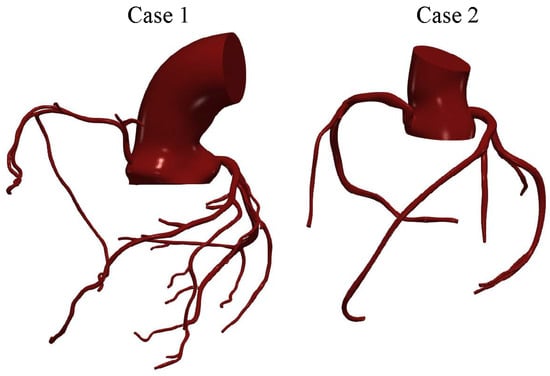
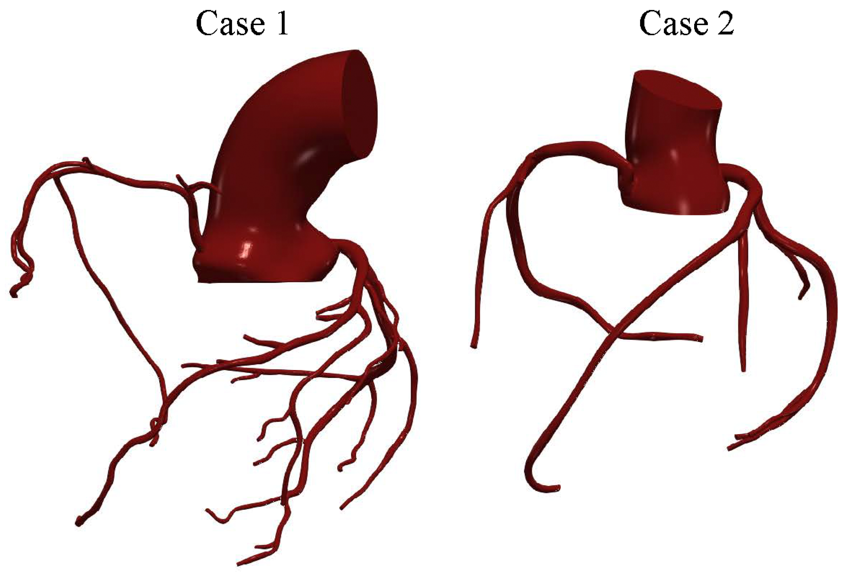
The two patient-specific aortic–coronary geometries and the associated haemodynamic data were obtained from previously published datasets [29]. The first case corresponds to the coronary arterial anatomy of a 63-year-old female subject (case 1), while the second case was obtained from a 28-year-old female subject (case 2). In both cases, the computational domains include the main coronary branches responsible for myocardial perfusion, namely the left main coronary artery (LMCA), the left anterior descending artery (LAD), the left circumflex artery (LCX), and the right coronary artery (RCA). The three-dimensional anatomical models were reconstructed from computed tomography (CT) data, allowing the major morphological characteristics of the coronary tree to be represented, including vessel curvature, bifurcations, and local variations in vessel diameter. A representation of the geometries investigated is reported in Figure 1.

Figure 1. Patient-specific coronary arterial geometries used in the simulations.

The resulting coronary geometries were discretised using the OpenFOAM utility snappyHexMesh. The meshes were refined in the near-wall region through the introduction of boundary-layer cells to improve the resolution of wall-adjacent gradients and the haemodynamic quantities of interest. For the fine grid, the background mesh had an average cell size of approximately $1\mathrm{mm}$, with a minimum local cell size of approximately $0.07\mathrm{mm}$ in the most refined regions. Boundary-layer cells had an initial height of $0.025\mathrm{mm}$.

A grid-sensitivity analysis was performed using three mesh configurations with different spatial resolutions. The finest grids consisted of approximately 5 million (Case 1) and 4.3 million (Case 2) elements, whereas two coarser grids were derived from the fine mesh by systematically removing every other node, resulting in approximately $6.0\times {10}^5$ and $7.5\times {10}^4$ elements for the medium and coarse grids of Case 1, and $5.3\times {10}^5$ and $6.7\times {10}^4$ elements for Case 2. The same meshing strategy was adopted for both patient-specific geometries to ensure a consistent comparison of the resulting haemodynamic fields.

For the numerical solution, spatial discretisation of the convective terms was performed using a blended linearUpwind scheme, while temporal integration was carried out using the Euler method. A variable time-step strategy was adopted to keep the Courant number below the prescribed value of $0.8$ throughout the simulation; on the fine grids, the resulting time step ranged between approximately $1.2\times {10}^{-5}$ and $3.6\times {10}^{-5}$ s over the cardiac cycle. The arterial walls were modelled as rigid and impermeable, and a no-slip condition was imposed at the wall boundaries. This common assumption was adopted because a fluid–structure interaction analysis of the present domains, combining small tortuous coronary vessels, large mesh deformations driven by cardiac motion, and ten simulated cardiac cycles, would be computationally prohibitive with currently available CFD tools. In a recent comparison between rigid-wall CFD and fluid–structure interaction for a patient-specific thoracic aorta [39], the pressure field differed by less than $1\%$, while the fluid–structure interaction simulation required about five times the computational cost even for that simpler geometry.

The Spalart–Allmaras detached eddy simulation (DES) [40,41] was adopted to account for possible turbulent and locally separated flow structures. This hybrid model switches between a pure LES approach in the core turbulent region, where large unsteady turbulence scales can be resolved by grid size, and a RANS Spalart–Allmaras model near solid walls, where the typical length scale of the turbulent eddies is significantly smaller than the grid dimensions. Based on the effective inlet diameter (≈35 and $30\mathrm{mm}$ for Case 1 and Case 2, respectively) and the cross-sectionally averaged velocity, the bulk inlet Reynolds number reaches approximately 2800 (Case 1) and 3500 (Case 2) at peak systole, with cycle-averaged values of approximately 760 and 870. However, the complex geometry of the aortic root and the coronary ostia generates local jets, separation and vortical structures, with local velocities of the order of $1\mathrm{m}{\mathrm{s}}^{-1}$; the corresponding local Reynolds number, based on the aortic diameter, approaches values of the order of ${10}^4$. Under these conditions, locally turbulent structures may develop during systolic deceleration, and the DES approach was therefore adopted. Where the flow is laminar, as in most of the coronary branches, or where the large scales are resolved, the modelled contribution remains small, as verified a posteriori in Section 3.1.

The inlet velocity profile was defined according to the power-law formulation described in the previous subsection. In the present case, the Womersley number associated with the aortic inlet was evaluated as

$$Wo=R_{\mathrm{eff}}\sqrt{{\displaystyle \frac{2\pi }{\nu T}}},$$

(24)

Using $\nu =4.0\times {10}^{-6}{\mathrm{m}}^2{\mathrm{s}}^{-1}$ and the case-specific inlet radius and cardiac-cycle period, the resulting Womersley numbers were approximately $Wo\simeq 22$ for Case 1 and $Wo\simeq 20.6$ for Case 2. This relatively high value indicates that unsteady inertial effects are relevant at the inlet and that the velocity profile is expected to be blunter than a quasi-steady parabolic profile. Accordingly, the power-law exponent was set to $n=9$, yielding

$$U_{\max }\left(t\right)={\displaystyle \frac{n+2}{n}}{\displaystyle \frac{Q\left(t\right)}{A_{\mathrm{in}}}}\simeq 1.22{\displaystyle \frac{Q\left(t\right)}{A_{\mathrm{in}}}},$$

(25)

which corresponds to a flattened inlet velocity distribution consistent with the estimated Womersley regime. For $Wo\simeq 20.6$–22, the thickness of the oscillatory (Stokes) boundary layer, $\delta =\sqrt{2\nu /\omega }=\sqrt{2}{R}_{\mathrm{eff}}/Wo$, is approximately $0.07R_{\mathrm{eff}}$, so that the Womersley solution exhibits a nearly flat core over most of the section. A pure plug profile, however, would introduce a velocity discontinuity at the wall and neglect the non-fully-developed character of the flow entering the aortic root. The value $n=9$ was therefore adopted as a compromise, yielding a blunt profile ($U_{\max }/\overline{U}\simeq 1.22$, compared with 2 for a parabolic profile and 1 for a plug profile) while retaining a smooth near-wall distribution. It is worth noting that the flow distribution among the coronary branches is mainly governed by the downstream impedance: the total coronary resistance (≈$3.8\times {10}^9\mathrm{Pa}\mathrm{s}{\mathrm{m}}^{-3}$) is about 24 times the systemic resistance, and the pressure drop across the three-dimensional coronary domain is a small fraction of the driving pressure. Variations of n within a plausible range (e.g., 7–11, corresponding to $U_{\max }/\overline{U}$ between $1.29$ and $1.18$) are therefore expected to affect mainly the local velocity distribution in the aortic root rather than the coronary flow partition.

The parameters adopted for the aortic Windkessel boundary condition are summarised in Table 1, while the outlet-specific parameters of the coronary lumped-parameter models are reported in Table 2 and Table 3.

Table 1. Parameters adopted for the aortic three-element Windkessel boundary condition.

Parameter	Symbol	Case 1	Case 2
Proximal resistance	$R_p$	$1.41\times {10}^7\mathrm{Pa}\mathrm{s}{\mathrm{m}}^{-3}$	$1.40\times {10}^7\mathrm{Pa}\mathrm{s}{\mathrm{m}}^{-3}$
Distal resistance	$R_d$	$1.43\times {10}^8\mathrm{Pa}\mathrm{s}{\mathrm{m}}^{-3}$	$1.42\times {10}^8\mathrm{Pa}\mathrm{s}{\mathrm{m}}^{-3}$
Compliance	C	$1.04\times {10}^{-8}{\mathrm{m}}^3{\mathrm{Pa}}^{-1}$	$9.78\times {10}^{-9}{\mathrm{m}}^3{\mathrm{Pa}}^{-1}$

Table 2. Case 1. Outlet-specific parameters adopted for the coronary lumped-parameter boundary conditions. Resistances are expressed in $\mathrm{Pa}\mathrm{s}{\mathrm{m}}^{-3}$ and compliances in ${\mathrm{m}}^3{\mathrm{Pa}}^{-1}$.

Outlet	${\mathit{R}}_{\mathit{a}}$	${\mathit{R}}_{\mathit{\text{a-micro}}}$	${\mathit{R}}_{\mathit{v}}+{\mathit{R}}_{\mathit{\text{v-micro}}}$	${\mathit{C}}_{\mathit{a}}$	${\mathit{C}}_{\mathit{im}}$
1	$5.63\times {10}^{10}$	$9.15\times {10}^{10}$	$2.82\times {10}^{10}$	$1.71\times {10}^{-12}$	$1.38\times {10}^{-11}$
2	$2.53\times {10}^{10}$	$4.11\times {10}^{10}$	$1.27\times {10}^{10}$	$3.16\times {10}^{-12}$	$2.56\times {10}^{-11}$
3	$3.69\times {10}^{10}$	$6.00\times {10}^{10}$	$1.84\times {10}^{10}$	$2.36\times {10}^{-12}$	$1.91\times {10}^{-11}$
4	$1.93\times {10}^{10}$	$3.14\times {10}^{10}$	$9.66\times {10}^9$	$3.89\times {10}^{-12}$	$3.15\times {10}^{-11}$
5	$1.15\times {10}^{10}$	$1.87\times {10}^{10}$	$5.76\times {10}^9$	$5.79\times {10}^{-12}$	$4.68\times {10}^{-11}$
6	$2.02\times {10}^{10}$	$3.29\times {10}^{10}$	$1.01\times {10}^{10}$	$3.75\times {10}^{-12}$	$3.04\times {10}^{-11}$
7	$2.80\times {10}^{10}$	$4.55\times {10}^{10}$	$1.40\times {10}^{10}$	$2.92\times {10}^{-12}$	$2.36\times {10}^{-11}$
8	$4.72\times {10}^{10}$	$7.67\times {10}^{10}$	$2.36\times {10}^{10}$	$1.96\times {10}^{-12}$	$1.58\times {10}^{-11}$
9	$3.10\times {10}^{10}$	$5.04\times {10}^{10}$	$1.55\times {10}^{10}$	$2.70\times {10}^{-12}$	$2.19\times {10}^{-11}$
10	$3.25\times {10}^{10}$	$5.28\times {10}^{10}$	$1.62\times {10}^{10}$	$2.61\times {10}^{-12}$	$2.11\times {10}^{-11}$
11	$5.07\times {10}^{10}$	$8.24\times {10}^{10}$	$2.54\times {10}^{10}$	$1.85\times {10}^{-12}$	$1.50\times {10}^{-11}$
12	$2.77\times {10}^{10}$	$4.50\times {10}^{10}$	$1.38\times {10}^{10}$	$2.95\times {10}^{-12}$	$2.39\times {10}^{-11}$
13	$3.31\times {10}^{10}$	$5.38\times {10}^{10}$	$1.66\times {10}^{10}$	$2.57\times {10}^{-12}$	$2.08\times {10}^{-11}$
14	$1.69\times {10}^{10}$	$2.74\times {10}^{10}$	$8.44\times {10}^9$	$4.31\times {10}^{-12}$	$3.49\times {10}^{-11}$
15	$3.91\times {10}^{10}$	$6.35\times {10}^{10}$	$1.95\times {10}^{10}$	$2.26\times {10}^{-12}$	$1.83\times {10}^{-11}$
16	$5.14\times {10}^{10}$	$8.35\times {10}^{10}$	$2.57\times {10}^{10}$	$1.83\times {10}^{-12}$	$1.48\times {10}^{-11}$
17	$2.20\times {10}^{10}$	$3.58\times {10}^{10}$	$1.10\times {10}^{10}$	$3.51\times {10}^{-12}$	$2.84\times {10}^{-11}$
18	$1.95\times {10}^{10}$	$3.17\times {10}^{10}$	$9.75\times {10}^9$	$3.86\times {10}^{-12}$	$3.12\times {10}^{-11}$
19	$2.03\times {10}^{10}$	$3.29\times {10}^{10}$	$1.01\times {10}^{10}$	$3.75\times {10}^{-12}$	$3.03\times {10}^{-11}$
20	$4.02\times {10}^{10}$	$6.54\times {10}^{10}$	$2.01\times {10}^{10}$	$2.21\times {10}^{-12}$	$1.79\times {10}^{-11}$
21	$4.10\times {10}^{10}$	$6.67\times {10}^{10}$	$2.05\times {10}^{10}$	$2.18\times {10}^{-12}$	$1.76\times {10}^{-11}$
22	$1.02\times {10}^{11}$	$1.65\times {10}^{11}$	$5.09\times {10}^{10}$	$1.08\times {10}^{-12}$	$8.77\times {10}^{-12}$
23	$3.37\times {10}^{10}$	$5.47\times {10}^{10}$	$1.68\times {10}^{10}$	$2.54\times {10}^{-12}$	$2.05\times {10}^{-11}$
24	$7.70\times {10}^{10}$	$1.25\times {10}^{11}$	$3.85\times {10}^{10}$	$1.34\times {10}^{-12}$	$1.09\times {10}^{-11}$

Table 3. Case 2. Outlet-specific parameters adopted for the coronary lumped-parameter boundary conditions. Resistances are expressed in $\mathrm{Pa}\mathrm{s}{\mathrm{m}}^{-3}$ and compliances in ${\mathrm{m}}^3{\mathrm{Pa}}^{-1}$.

Outlet	${\mathit{R}}_{\mathit{a}}$	${\mathit{R}}_{\mathit{\text{a-micro}}}$	${\mathit{R}}_{\mathit{v}}+{\mathit{R}}_{\mathit{\text{v-micro}}}$	${\mathit{C}}_{\mathit{a}}$	${\mathit{C}}_{\mathit{im}}$
1	$7.00\times {10}^9$	$1.14\times {10}^{10}$	$3.50\times {10}^9$	$1.06\times {10}^{-11}$	$8.55\times {10}^{-11}$
2	$2.25\times {10}^{10}$	$3.65\times {10}^{10}$	$1.12\times {10}^{10}$	$4.31\times {10}^{-12}$	$3.49\times {10}^{-11}$
3	$1.01\times {10}^{10}$	$1.64\times {10}^{10}$	$5.05\times {10}^9$	$7.98\times {10}^{-12}$	$6.45\times {10}^{-11}$
4	$2.10\times {10}^{10}$	$3.42\times {10}^{10}$	$1.05\times {10}^{10}$	$4.54\times {10}^{-12}$	$3.67\times {10}^{-11}$
5	$1.31\times {10}^{10}$	$2.13\times {10}^{10}$	$6.55\times {10}^9$	$6.53\times {10}^{-12}$	$5.28\times {10}^{-11}$
6	$2.55\times {10}^{10}$	$4.14\times {10}^{10}$	$1.27\times {10}^{10}$	$3.91\times {10}^{-12}$	$3.17\times {10}^{-11}$
7	$6.05\times {10}^9$	$9.83\times {10}^9$	$3.03\times {10}^9$	$1.18\times {10}^{-11}$	$9.57\times {10}^{-11}$
8	$8.32\times {10}^9$	$1.35\times {10}^{10}$	$4.16\times {10}^9$	$9.26\times {10}^{-12}$	$7.49\times {10}^{-11}$
9	$9.81\times {10}^9$	$1.59\times {10}^{10}$	$4.90\times {10}^9$	$8.16\times {10}^{-12}$	$6.60\times {10}^{-11}$

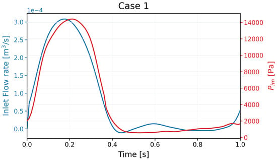
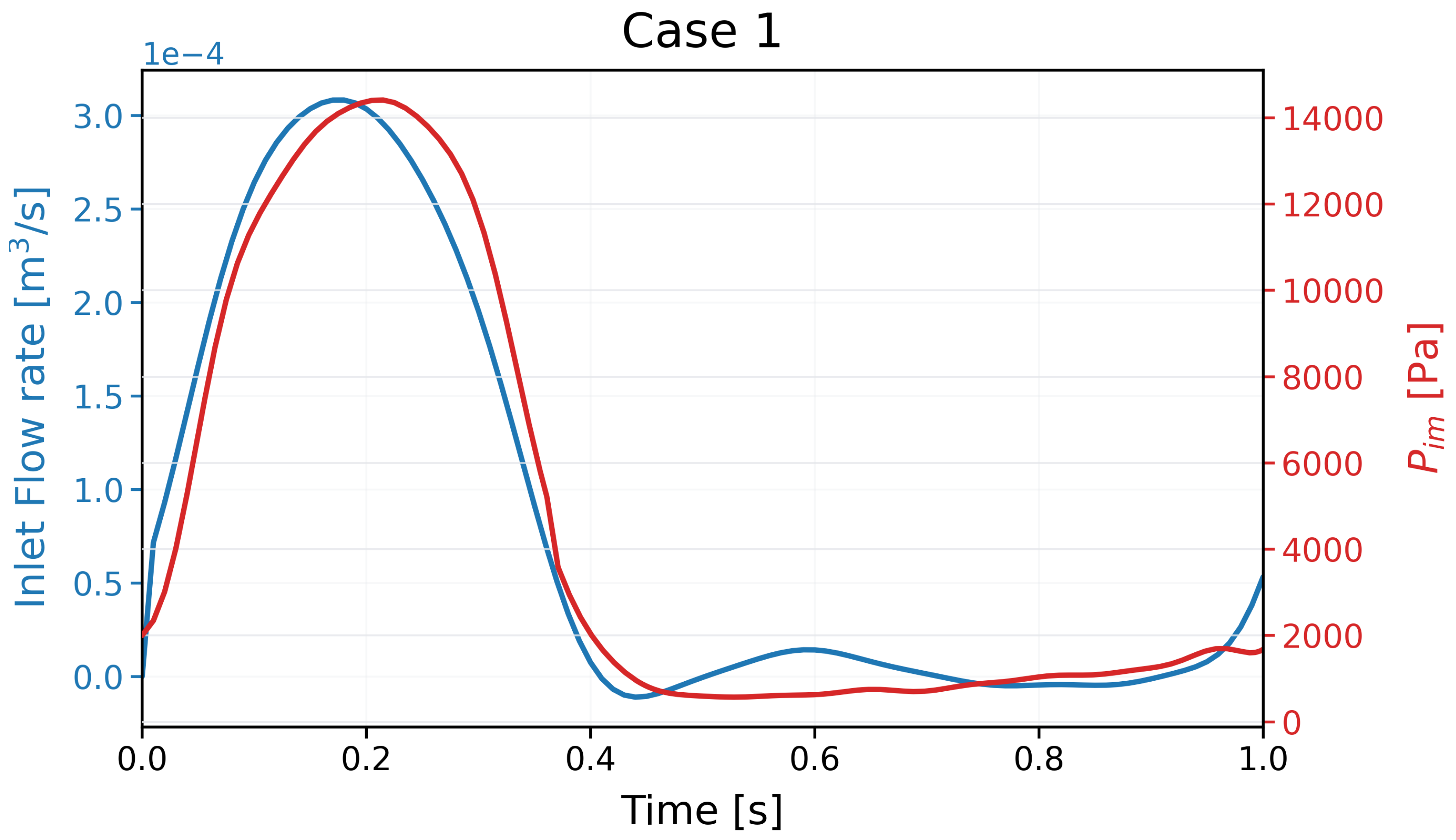
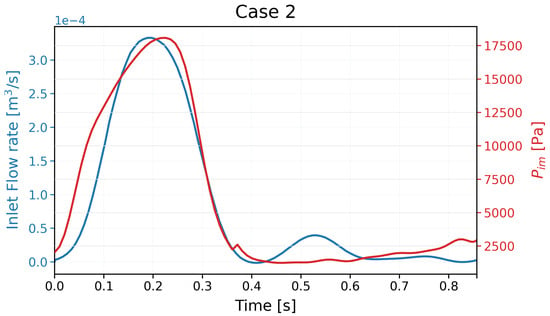
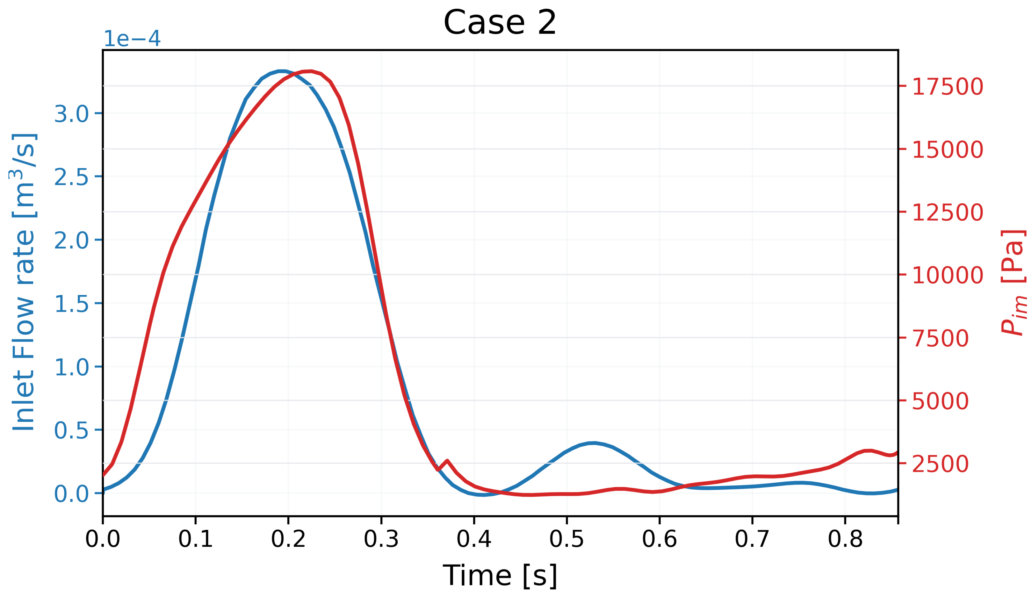
The following Figure 2 and Figure 3 show the time-dependent inlet flow rate and intramyocardial pressure adopted for the two investigated cases.

Figure 2. Inlet flow rate and intramyocardial pressure $P_{im}$ prescribed for Case 1 over a cardiac cycle.

Figure 3. Inlet flow rate and intramyocardial pressure $P_{im}$ prescribed for Case 2 over a cardiac cycle.

Ten cardiac cycles were simulated to allow the coupled three-dimensional and lumped-parameter models to reach a periodic state. The results presented in the following sections refer to the subsequent cardiac cycle.

3. Results

3.1. Grid-Sensitivity and Discretisation-Uncertainty Study

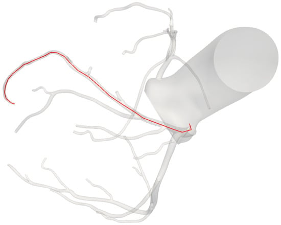
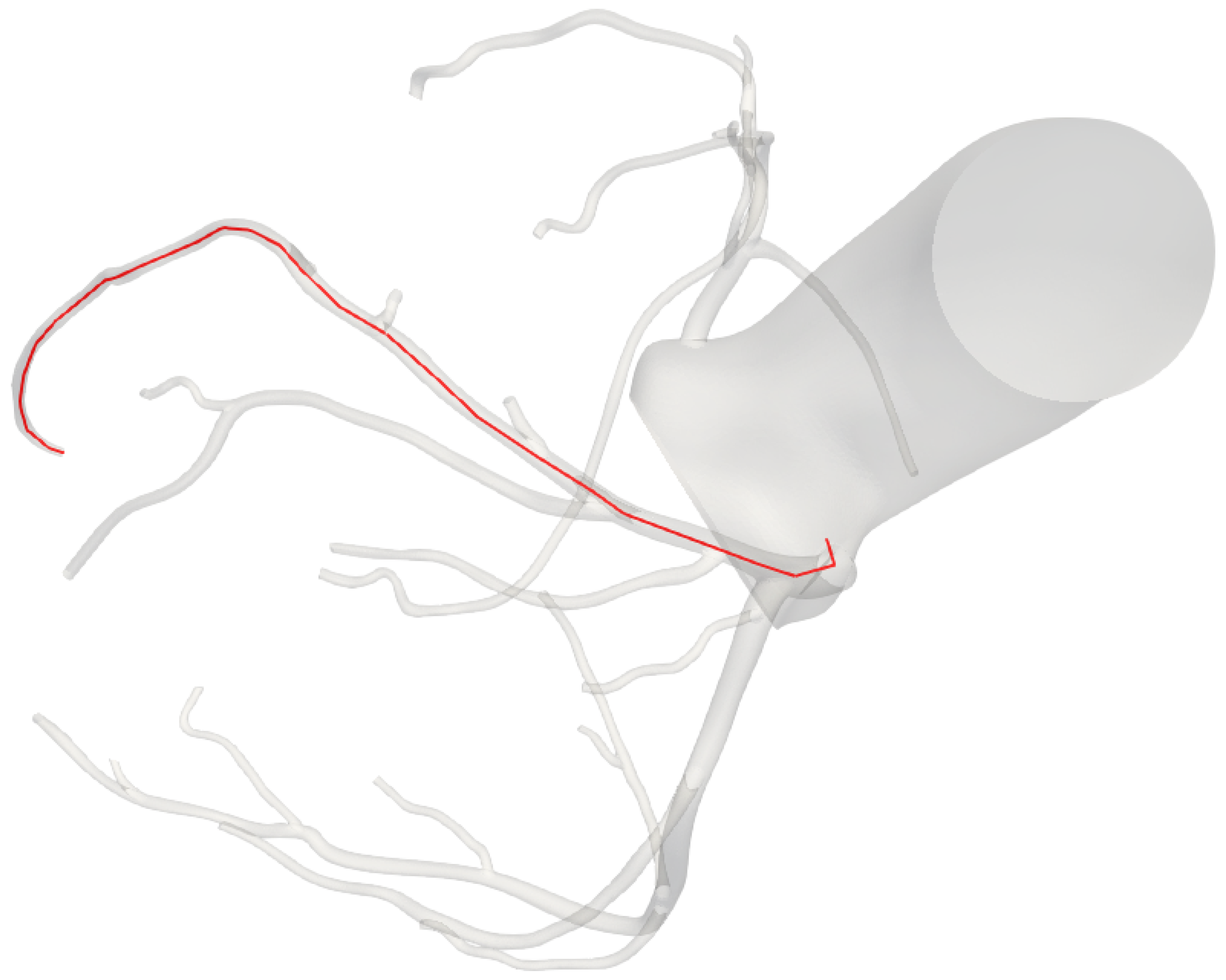
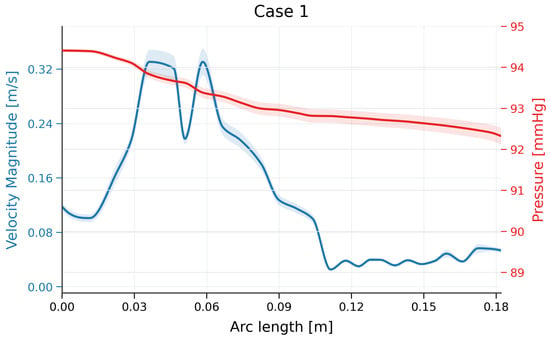
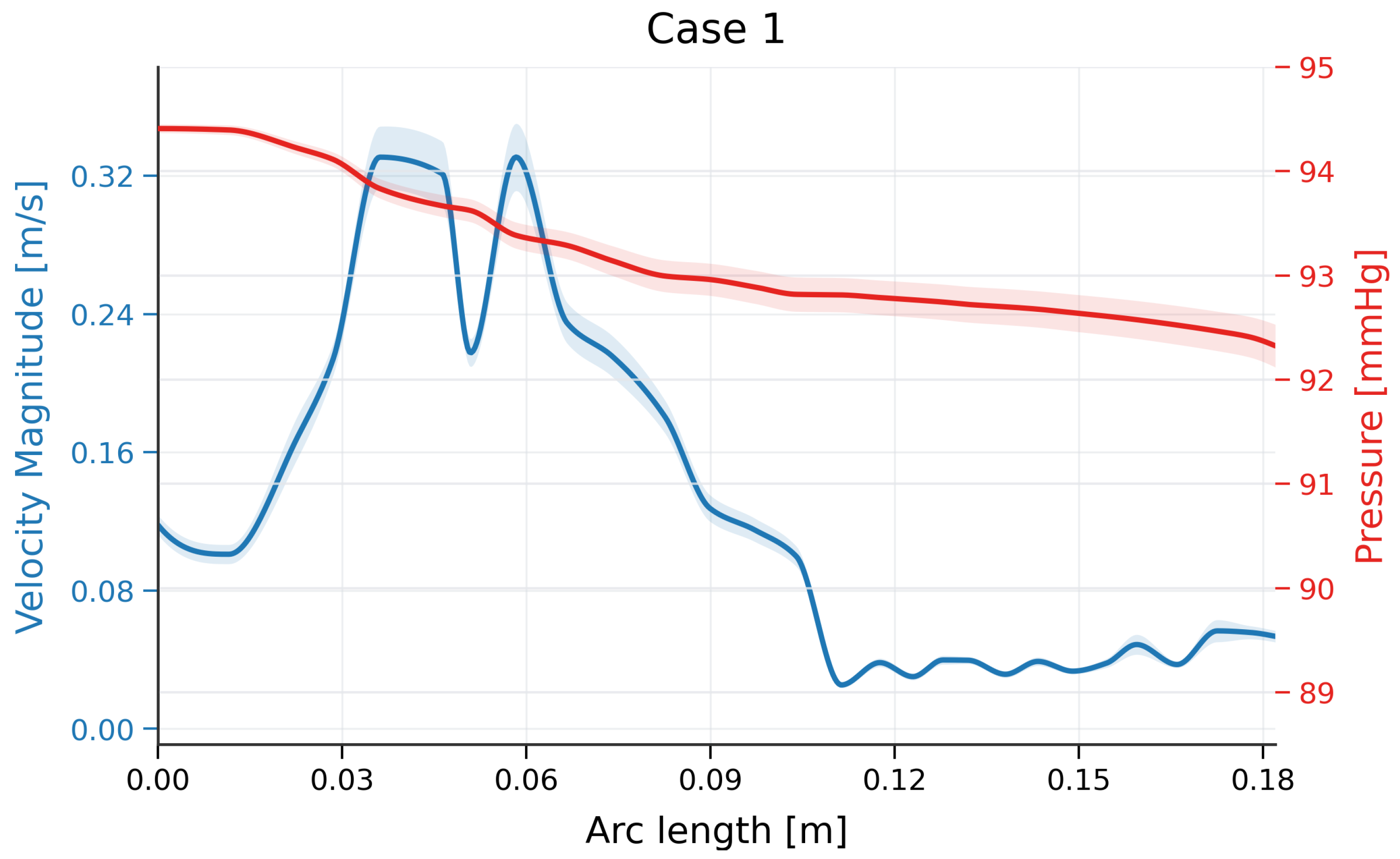
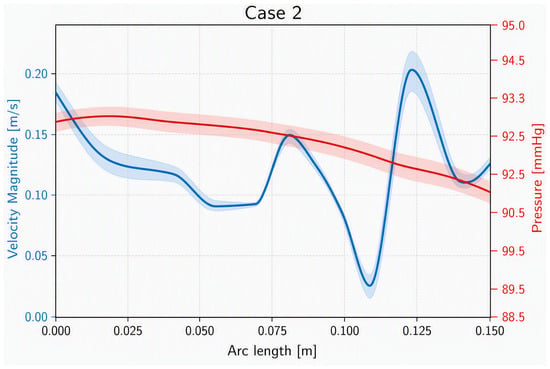
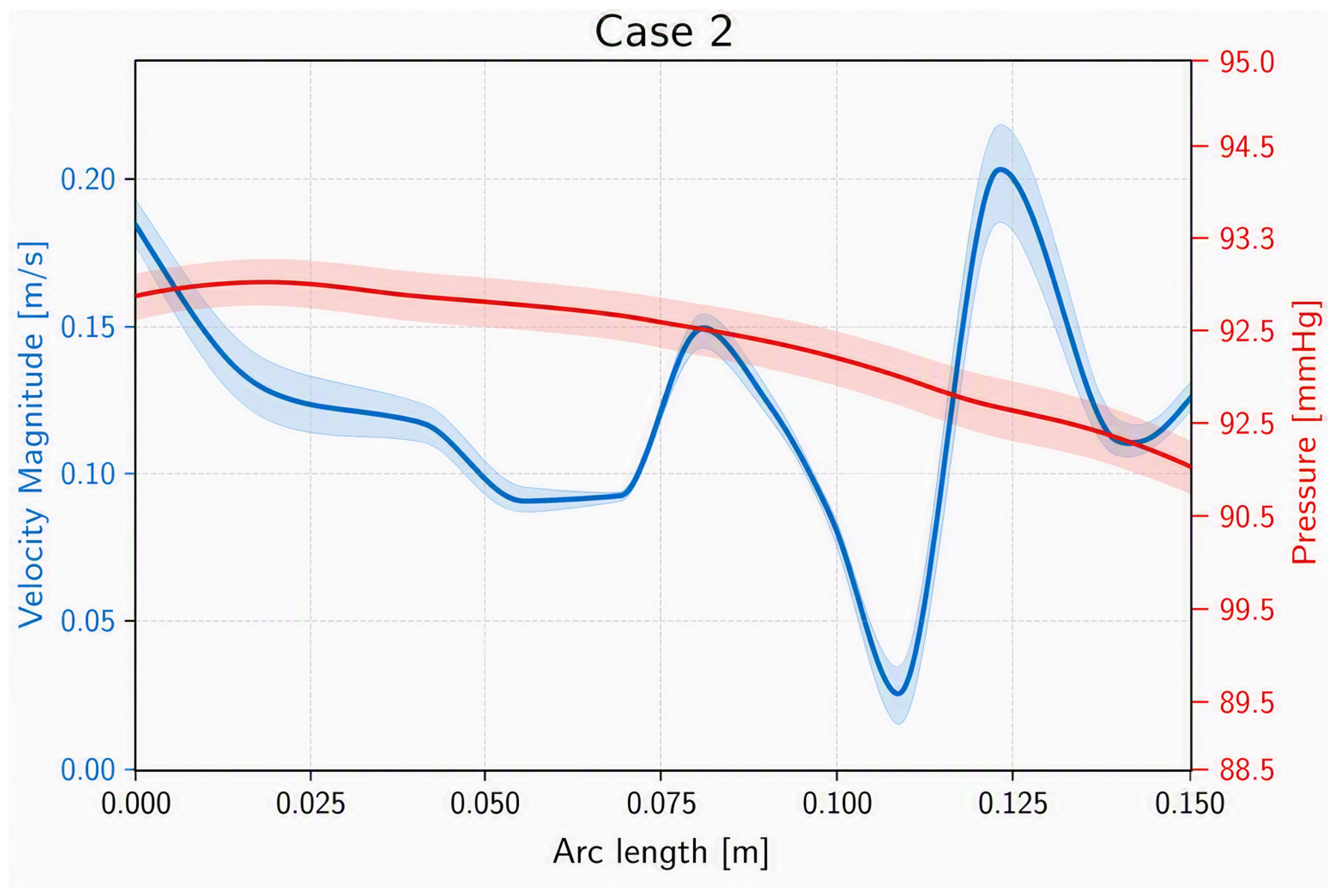
The numerical uncertainty associated with the simulations performed was estimated using the framework proposed by Roache [42,43]. The analysis was performed for the two investigated cases using the mean pressure and the mean velocity magnitude during a heartbeat sampled along a representative coronary centreline. Figure 4 shows the centreline for case 1; the centreline for case 2 is similar and is omitted for brevity.

Figure 4. Representative coronary centreline for Case 1.

Figure 5 and Figure 6 show the fine-grid profiles and the corresponding local uncertainty bands.

Figure 5. Mean velocity magnitude and mean pressure along the selected coronary path for Case 1. The shaded regions represent the local numerical uncertainty.

Figure 6. Mean velocity magnitude and mean pressure along the selected coronary path for Case 2. The shaded regions represent the local numerical uncertainty.

To provide a compact quantitative comparison, the local relative GCI values were averaged over the sampled path. The maximum local value is also reported to identify regions exhibiting greater sensitivity to mesh refinement. The results are summarised in Table 4.

Table 4. Path-averaged and maximum local relative GCI for the mean velocity magnitude and mean pressure. The values were calculated using a safety factor of 3 and a refinement ratio of 2.

Case	Haemodynamic Quantity	Mean GCI [%]	Maximum GCI [%]
Case 1	Mean velocity magnitude, $\overline{\left|\mathbf{U}\right|}$	1.19	3.83
Case 1	Mean pressure, $\overline{p}$	0.16	0.22
Case 2	Mean velocity magnitude, $\overline{\left|\mathbf{U}\right|}$	0.91	2.55
Case 2	Mean pressure, $\overline{p}$	1.12	2.21

The low uncertainty indicates that the fine mesh is sufficient to accurately reproduce the behaviour of the main haemodynamic parameters; therefore, the results obtained with this grid were adopted as the reference solution. Near-wall quantities such as wall shear stress were not included in this assessment.

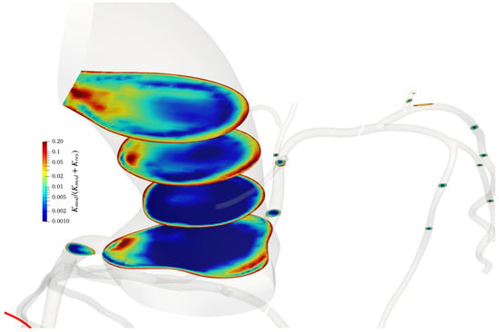
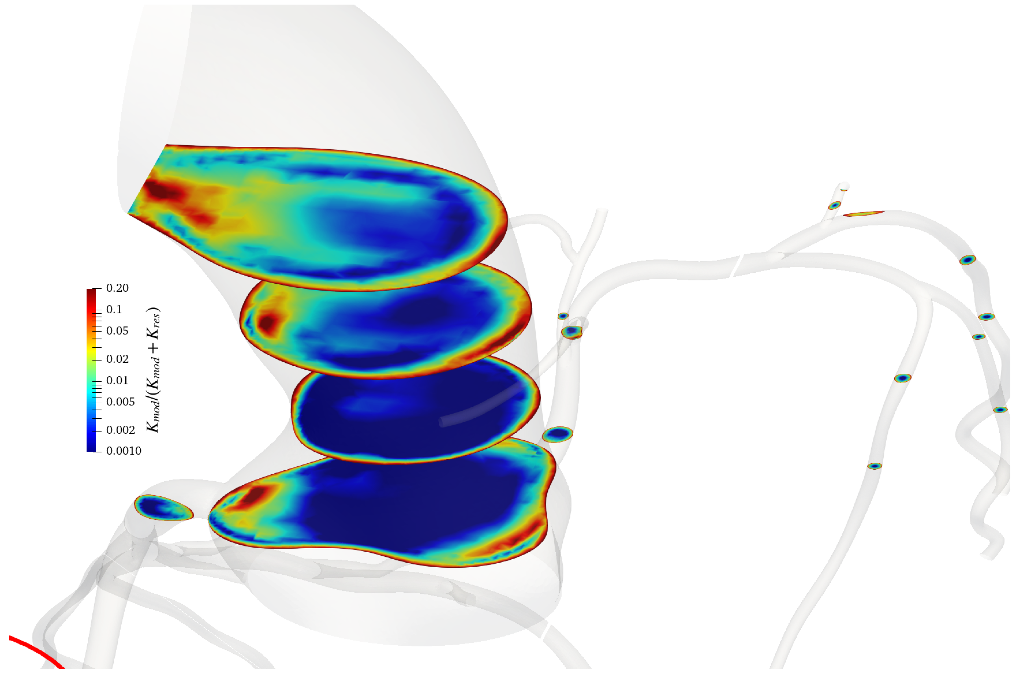
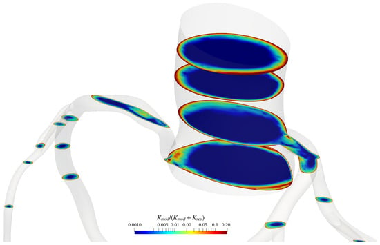
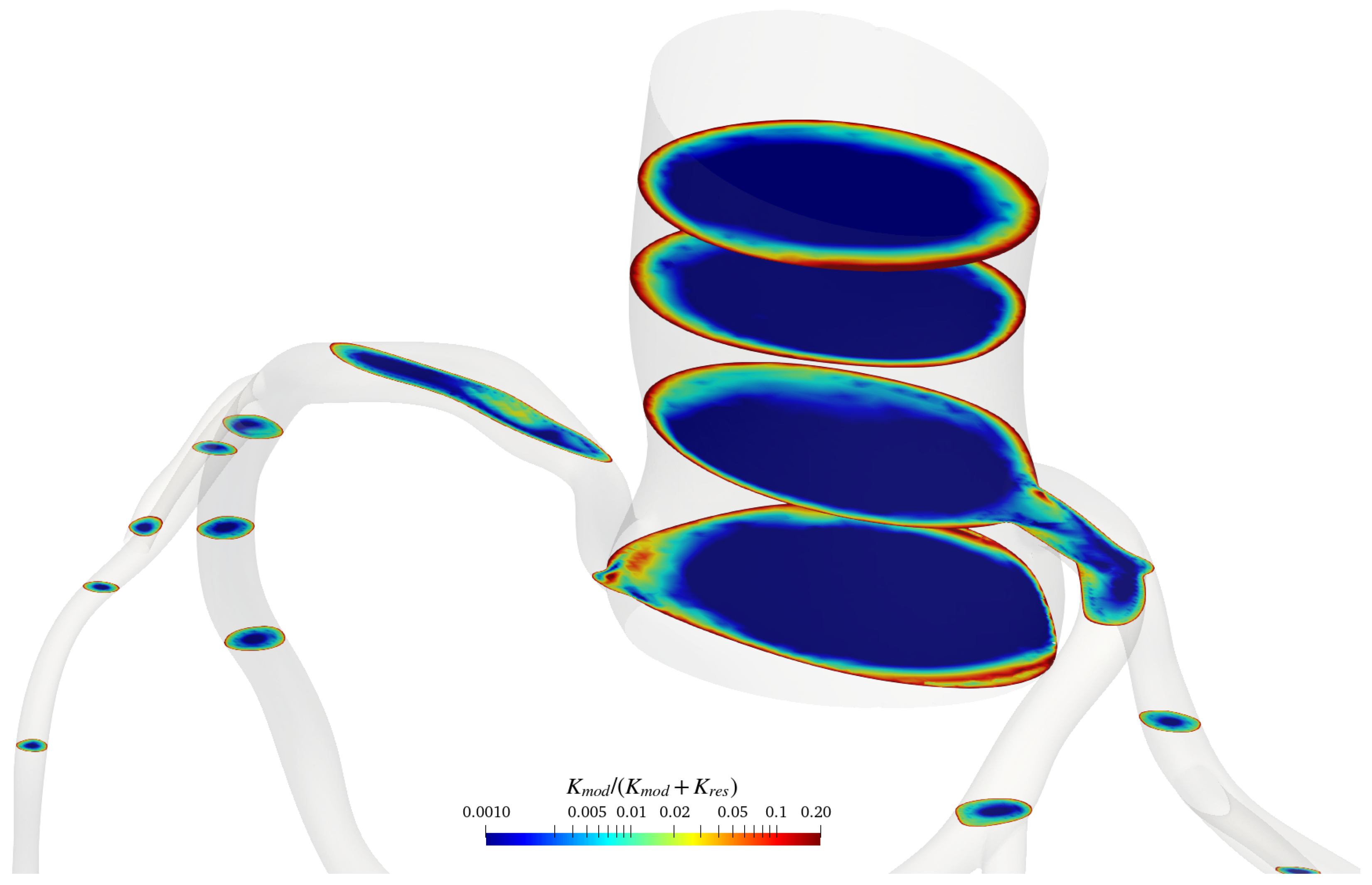
To assess the adequacy of the spatial resolution in regions where the turbulence model operates in large-eddy simulation mode, the modelled kinetic energy was compared with the total kinetic energy following the approach of Di Mascio et al. [44]. The resolved and modelled contributions were evaluated using the ratio

$${\chi }_K={\displaystyle \frac{K_{\mathrm{mod}}}{K_{\mathrm{mod}}+K_{\mathrm{res}}}},$$

(26)

where $K_{\mathrm{mod}}$ and $K_{\mathrm{res}}$ denote the modelled and resolved kinetic-energy contributions, respectively. Figure 7 and Figure 8 show the distribution of ${\chi }_K$ on representative cross-sections of the coronary arterial domains using cycle-averaged values.

Figure 7. Ratio of the modelled kinetic energy to the total kinetic energy, $K_{\mathrm{mod}}/(K_{\mathrm{mod}}+K_{\mathrm{res}})$, on representative cross-sections of the coronary arterial domain for case 1. The ratio is computed with cycle averaged values.

Figure 8. Ratio of the modelled kinetic energy to the total kinetic energy, $K_{\mathrm{mod}}/(K_{\mathrm{mod}}+K_{\mathrm{res}})$, on representative cross-sections of the coronary arterial domain for case 2. The ratio is computed with cycle averaged values.

The modelled kinetic-energy contribution remained smaller than the resolved contribution throughout most of the bulk-flow region. In particular, the ratio $K_{\mathrm{mod}}/(K_{\mathrm{mod}}+K_{\mathrm{res}})$ was below $0.2$ over most of the analysed sections, indicating that a sufficiently large fraction of the turbulent kinetic energy was directly resolved by the computational grid according to the criterion proposed by Pope [45]. Values exceeding $0.2$ were primarily confined to the near-wall region, where the turbulence formulation operates in its Reynolds-averaged mode. Overall, these results indicate that the adopted grid provides an adequate spatial resolution for the present coronary artery simulations.

3.2. Discussion of the Results

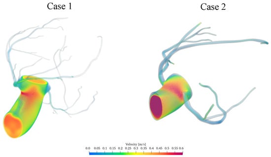
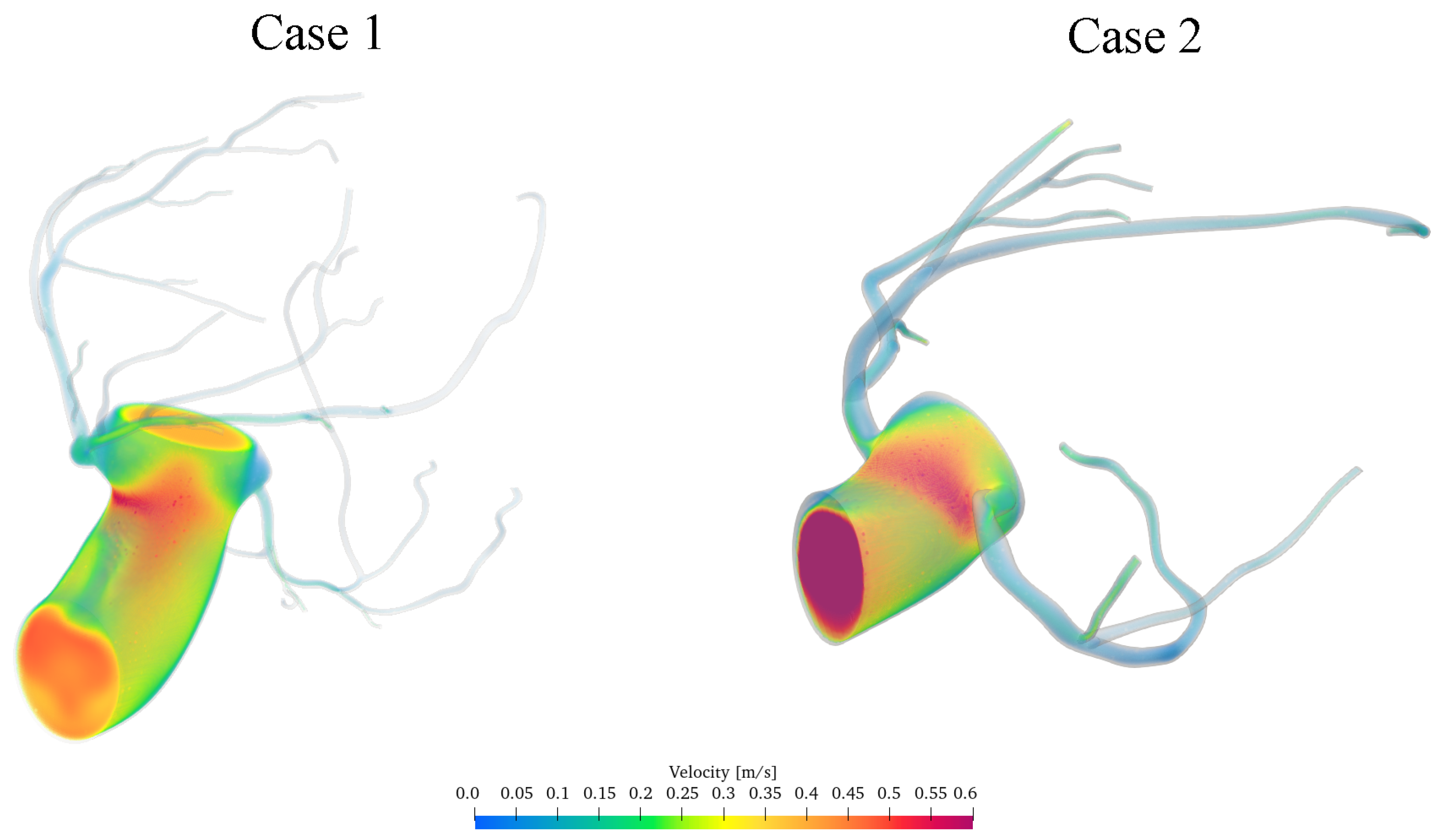
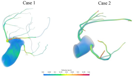
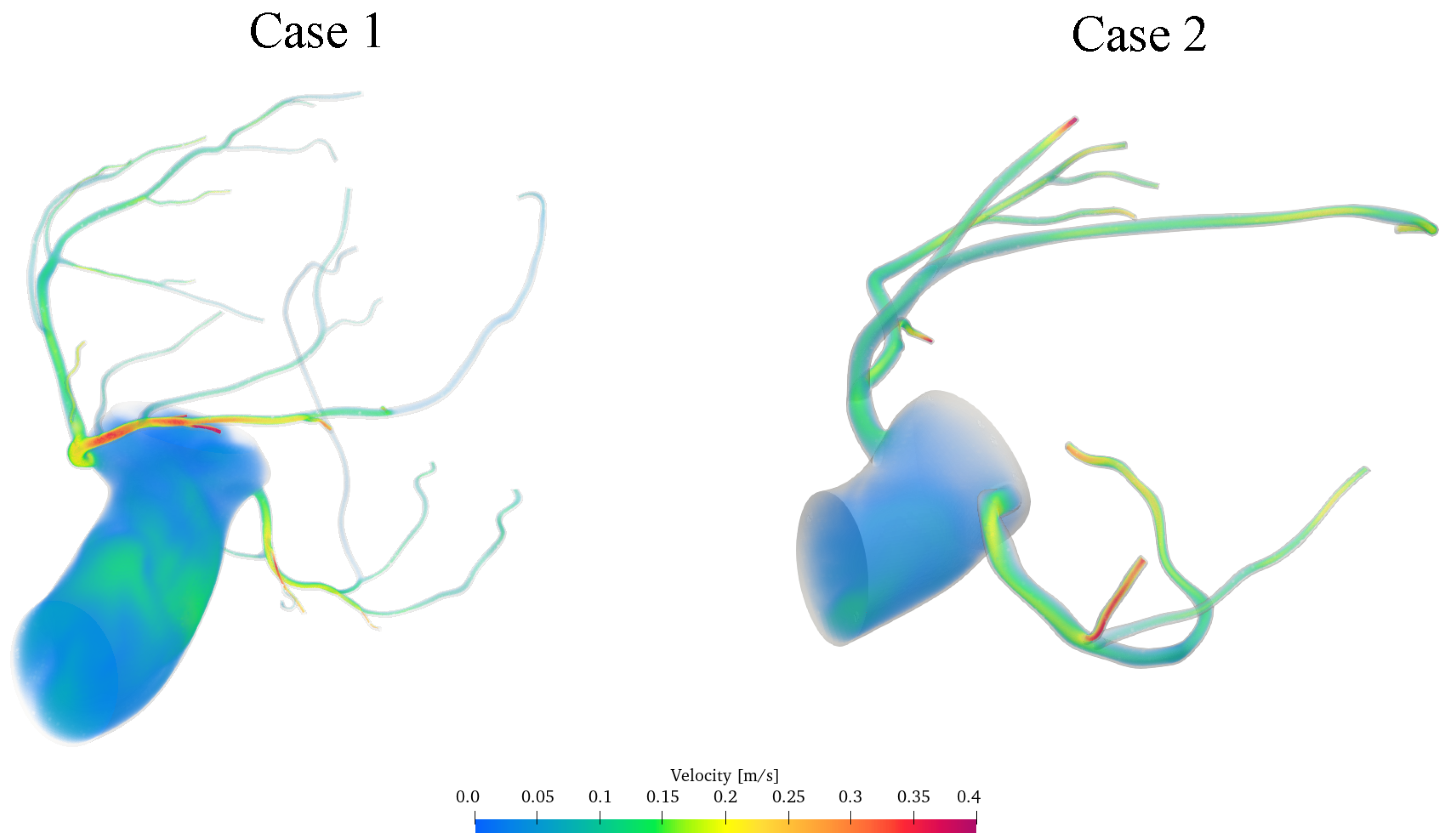
Figure 9 and Figure 10 present three-dimensional representations of the instantaneous velocity field within the two patient-specific coronary arterial geometries at the phases of systole, and diastole, respectively.

Figure 9. Computed instantaneous velocity-magnitude fields in the aortic–coronary domains investigated during systole.

Figure 10. Computed instantaneous velocity-magnitude fields in the aortic–coronary domains investigated during diastole.

Since patient-specific in vivo measurements (e.g., pressure-wire, fractional flow reserve or intracoronary Doppler data) were not available for the two anatomies, the following comparison assesses physiological plausibility rather than patient-specific accuracy. The predicted velocity magnitudes and their temporal variations are physiologically plausible and of the same order as those reported by previous in vivo Doppler measurements of coronary flow [46,47,48], as quantified in Table 5. The corresponding instantaneous velocity field during diastole is shown in Figure 10.

During diastole, locally increased velocity magnitudes are observed in several distal coronary branches. This behaviour is physiologically consistent with the enhanced coronary perfusion associated with ventricular relaxation and reflects the phase-dependent response introduced by the coronary outlet model.

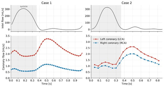
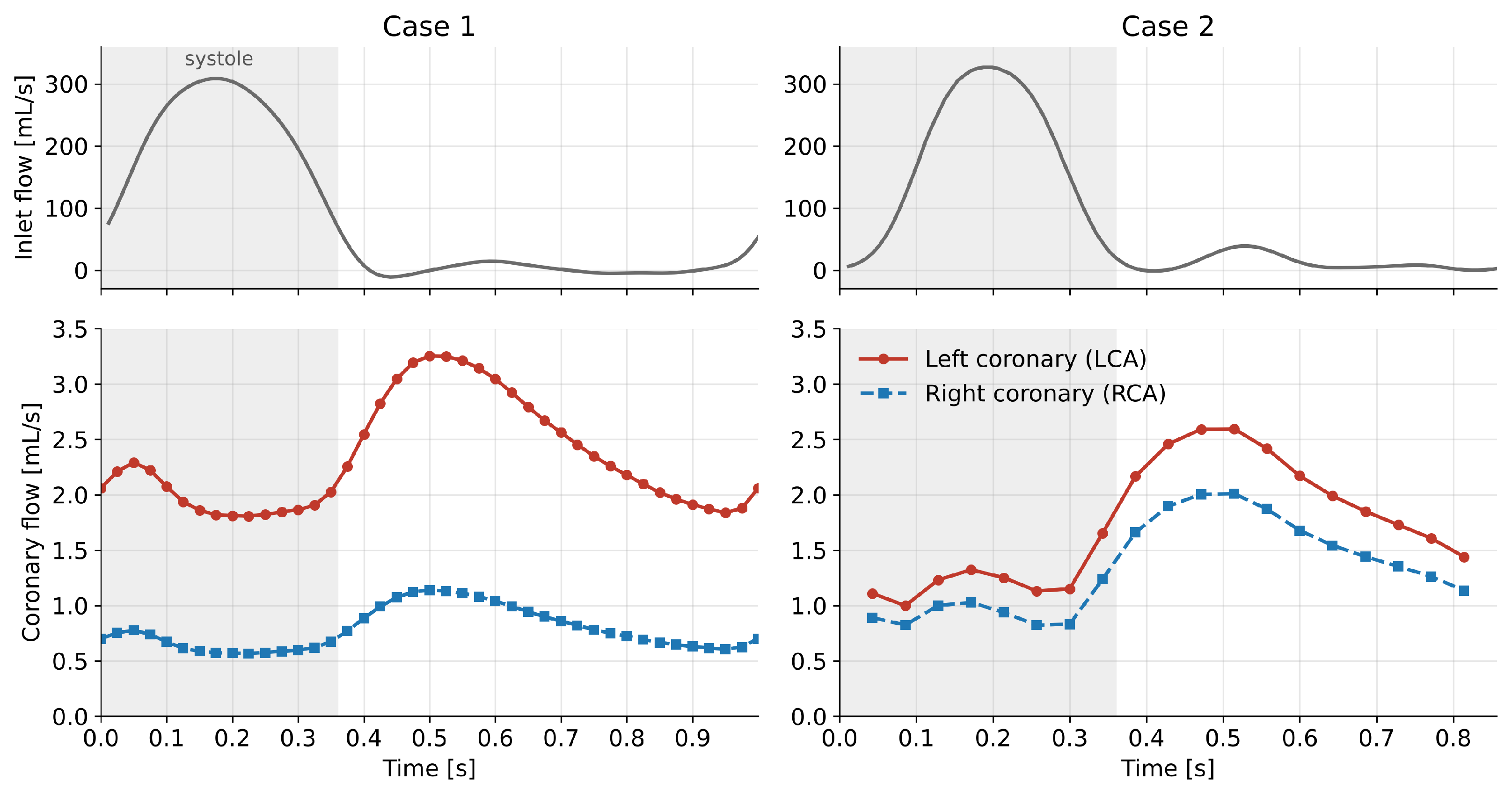
A quantitative summary of the computed haemodynamic quantities and of the corresponding reference values reported in the literature is given in Table 5. Cycle-averaged aortic and distal coronary pressures fall within the ranges measured invasively at rest. The computed coronary flow amounts to approximately $4.7\%$ of the inlet flow in both cases, close to the 4–$5\%$ of cardiac output typically received by the coronary circulation and consistent with the total coronary resistance prescribed in Equation (19). The left/right flow partition (approximately $75/25$ in Case 1 and $56/44$ in Case 2) lies within the range reported in vivo, which depends on coronary dominance [49]. The cycle-averaged velocity in the proximal left coronary artery ($0.16$–$0.17\mathrm{m}{\mathrm{s}}^{-1}$) is of the same order as, though lower than, the resting average peak velocity measured with intracoronary Doppler [50], which refers to the peak of the velocity spectrum; peak coronary velocities of $0.49$ (Case 1) and $0.29\mathrm{m}{\mathrm{s}}^{-1}$ (Case 2) are reached in early diastole. The time evolution of the coronary flow rate is shown in Figure 11: in both cases coronary flow peaks in early diastole, at approximately twice its systolic value, as expected from the phase-dependent action of the intramyocardial pressure.

Figure 11. Inlet flow rate (top) and left and right coronary flow rates (bottom) over the cardiac cycle for Case 1 (left) and Case 2 (right). The shaded region indicates systole.

Table 5. Computed haemodynamic quantities compared with reference ranges reported in the literature.

Quantity	Case 1	Case 2	Reference
Cycle-averaged aortic pressure [mmHg]	94.3	91.9	79–121 [48]
Cycle-averaged distal coronary pressure [mmHg]	92.3	90.2	73–114 [48]
Cycle-averaged proximal LCA velocity [m ${\mathrm{s}}^{-1}$]	0.17	0.16	0.22 ± ${0.08 }^a$ [50]
Coronary flow/inlet flow [%]	4.7	4.7	≈4–5 [1]
Left/right coronary flow [%]	75/25	56/44	58/42–78/${22 }^b$ [49]

^a Resting average peak velocity (intracoronary Doppler). ^b Right-dominant and left-dominant/balanced circulation, respectively.

Table 5. Computed haemodynamic quantities compared with reference ranges reported in the literature.

Quantity	Case 1	Case 2	Reference
Cycle-averaged aortic pressure [mmHg]	94.3	91.9	79–121 [48]
Cycle-averaged distal coronary pressure [mmHg]	92.3	90.2	73–114 [48]
Cycle-averaged proximal LCA velocity [m ${\mathrm{s}}^{-1}$]	0.17	0.16	0.22 ± ${0.08 }^a$ [50]
Coronary flow/inlet flow [%]	4.7	4.7	≈4–5 [1]
Left/right coronary flow [%]	75/25	56/44	58/42–78/${22 }^b$ [49]

^a Resting average peak velocity (intracoronary Doppler). ^b Right-dominant and left-dominant/balanced circulation, respectively.

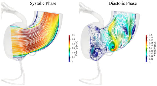
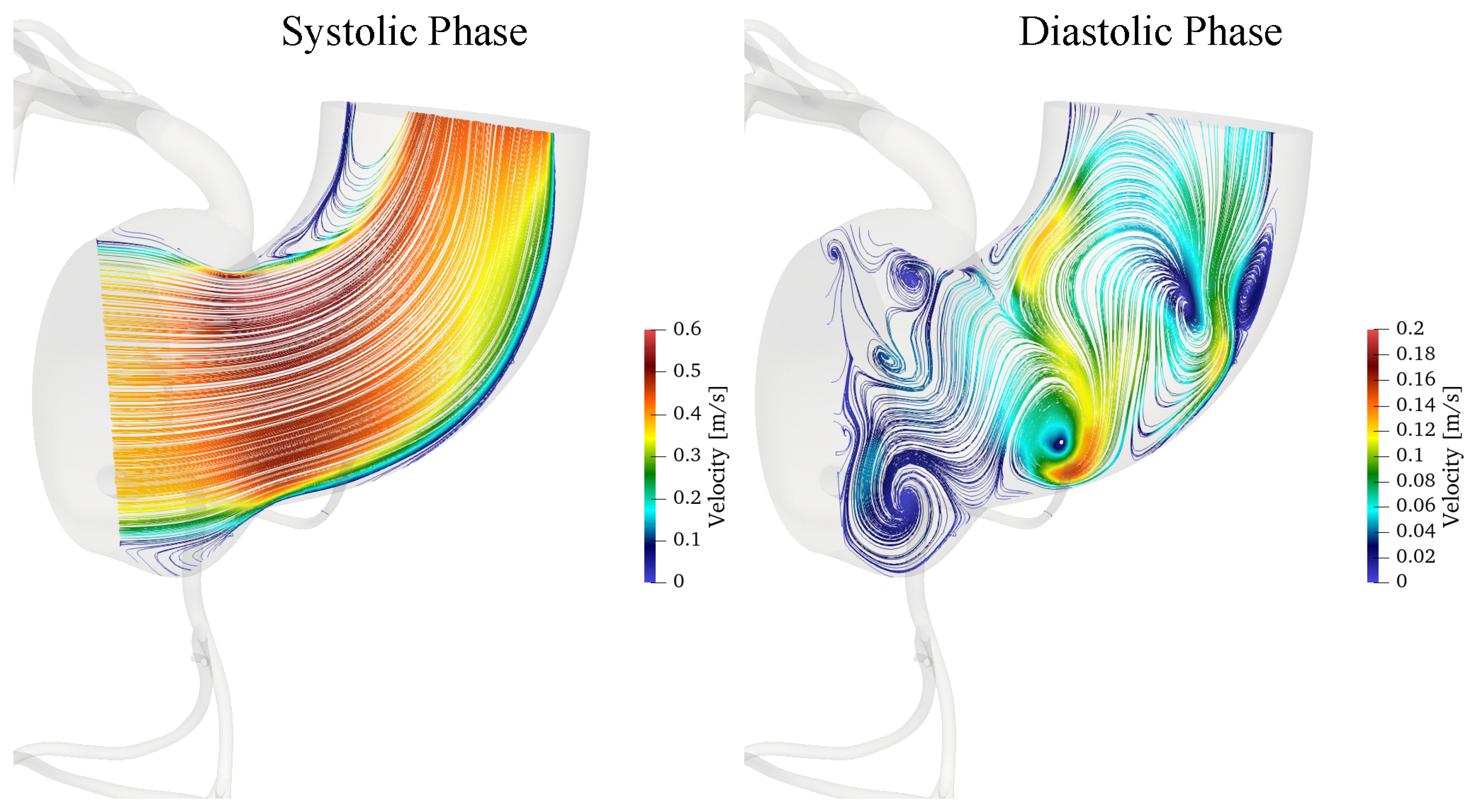
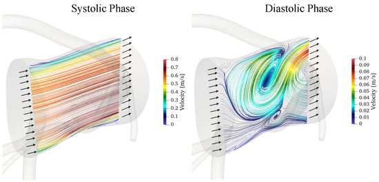
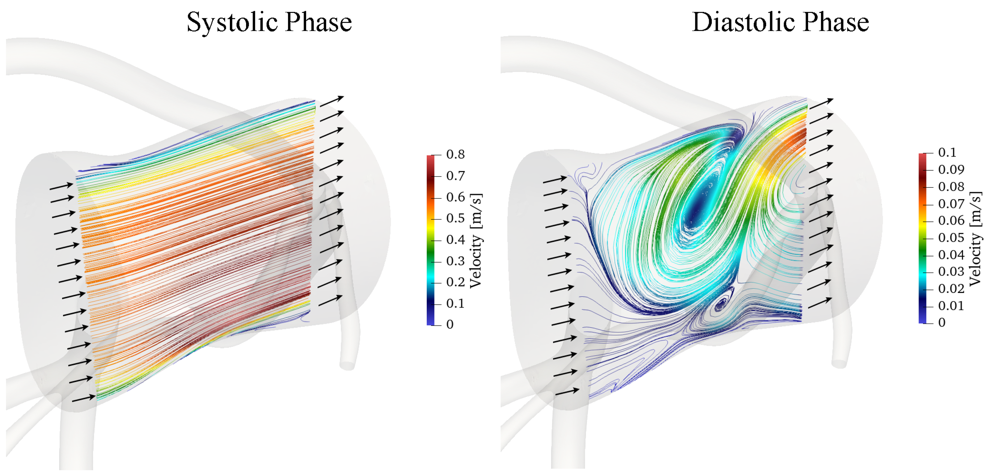
Figure 12 depicts velocity’s streamlines during systole and diastole phases for case 1.

Figure 12. Instantaneous velocity streamlines during systole and diastole for Case 1, coloured by the local velocity magnitude.

The results reveal marked differences in the coronary flow field between the two phases of the cardiac cycle. During systole, the higher velocity magnitude, reaching approximately $0.6\mathrm{m}{\mathrm{s}}^{-1}$, is associated with a coherent streamline pattern and a single localised recirculation vortex near the inner curvature. This vortex is associated with local flow deceleration and separation, promoted by the vessel curvature and the adverse pressure gradient in this region, as also indicated by the pressure fields presented below. The vortex forms near peak systole (at approximately $0.175$ s), grows during systolic deceleration and reaches its maximum extent at the end of ejection (at approximately $0.375$ s), when the reversed flow occupies about $60\%$ of the inner half of the section, with axial velocities down to $-0.35\mathrm{m}{\mathrm{s}}^{-1}$. It then breaks down into the multiple smaller structures described below by approximately $0.40$ s; it is therefore a transient systolic feature, lasting about $0.2$ s, rather than a persistent structure over the cardiac cycle.

During diastole, the lower velocities, up to approximately $0.2\mathrm{m}{\mathrm{s}}^{-1}$, are accompanied by multiple recirculation regions and more complex vortical structures. These differences reflect the combined effects of flow pulsatility and vessel curvature on the balance between inertial and pressure forces. Such disturbed-flow regions may produce spatial and temporal variations in wall shear stress, which are relevant to endothelial function and the local development of atherosclerotic disease. A detailed analysis of wall shear stress-based indicators, such as the time-averaged wall shear stress and the oscillatory shear index, is beyond the scope of the present work, focused on the solver and its boundary conditions, and will be addressed in future studies.

Figure 13 presents the instantaneous velocity streamlines obtained for Case 2 during systole and diastole.

Figure 13. Instantaneous velocity streamlines during systole and diastole for Case 2, coloured by the local velocity magnitude.

The flow behaviour observed for Case 2 is generally consistent with that described for Case 1. However, the different geometry of this coronary artery, and particularly the absence of a pronounced curvature, limits curvature-induced flow separation and consequently inhibits the formation of the localised inner-curvature vortex observed in Case 1. As a result, the flow field in Case 2 exhibits a more organised streamline distribution, with less pronounced recirculation in the corresponding region.

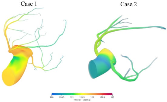
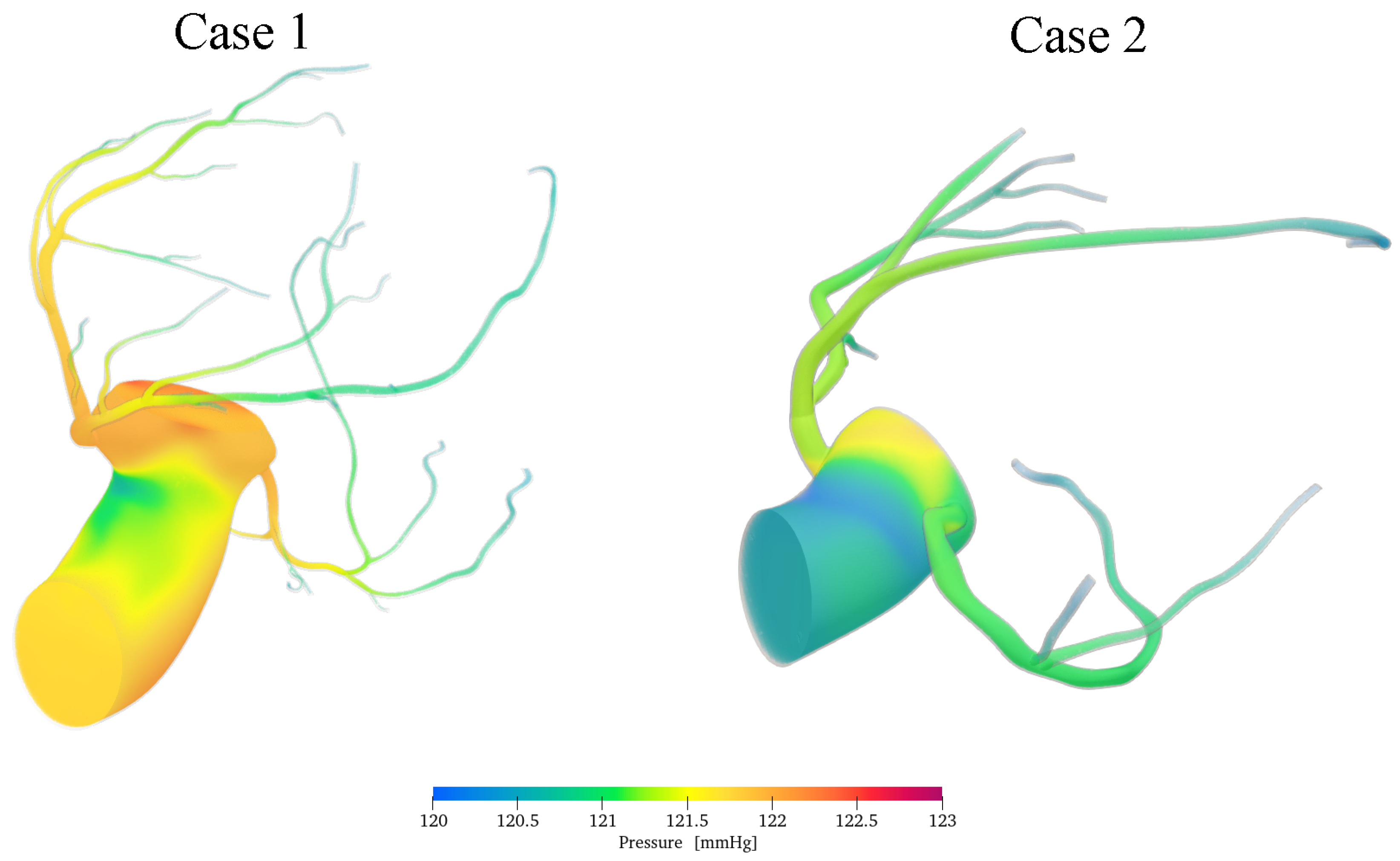
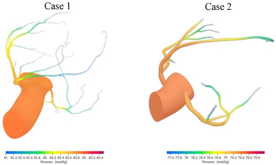
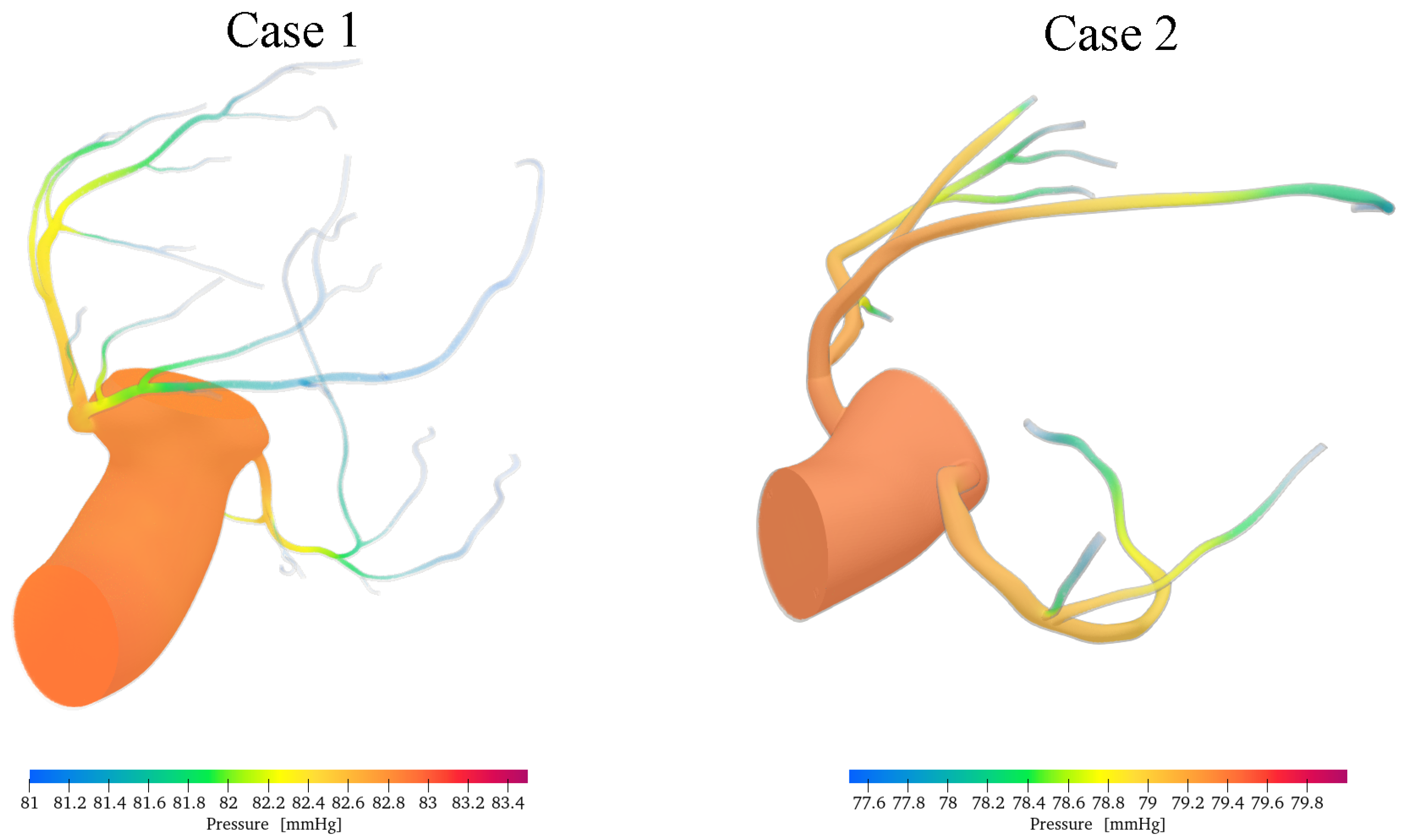
The instantaneous pressure fields provide further insight into the distinct haemodynamic behaviour of the aortic and coronary flow pathways. Figure 14 and Figure 15 show the pressure distribution within the computational domain during systole and diastole, respectively. The colour scale reports the local pressure in mmHg.

Figure 14. Computed pressure fields in the aortic and coronary domains during systole.

Figure 15. Computed pressure fields in the aortic and coronary domains during diastole.

The computed pressure magnitudes are consistent with the overall pressure scale reported by invasive measurements, which yielded cycle-averaged resting aortic and distal coronary pressures of 79–$121\mathrm{mmHg}$ and 73–$114\mathrm{mmHg}$, respectively, under different haemodynamic conditions [48]. The corresponding pressure field during diastole is shown in Figure 15.

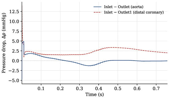
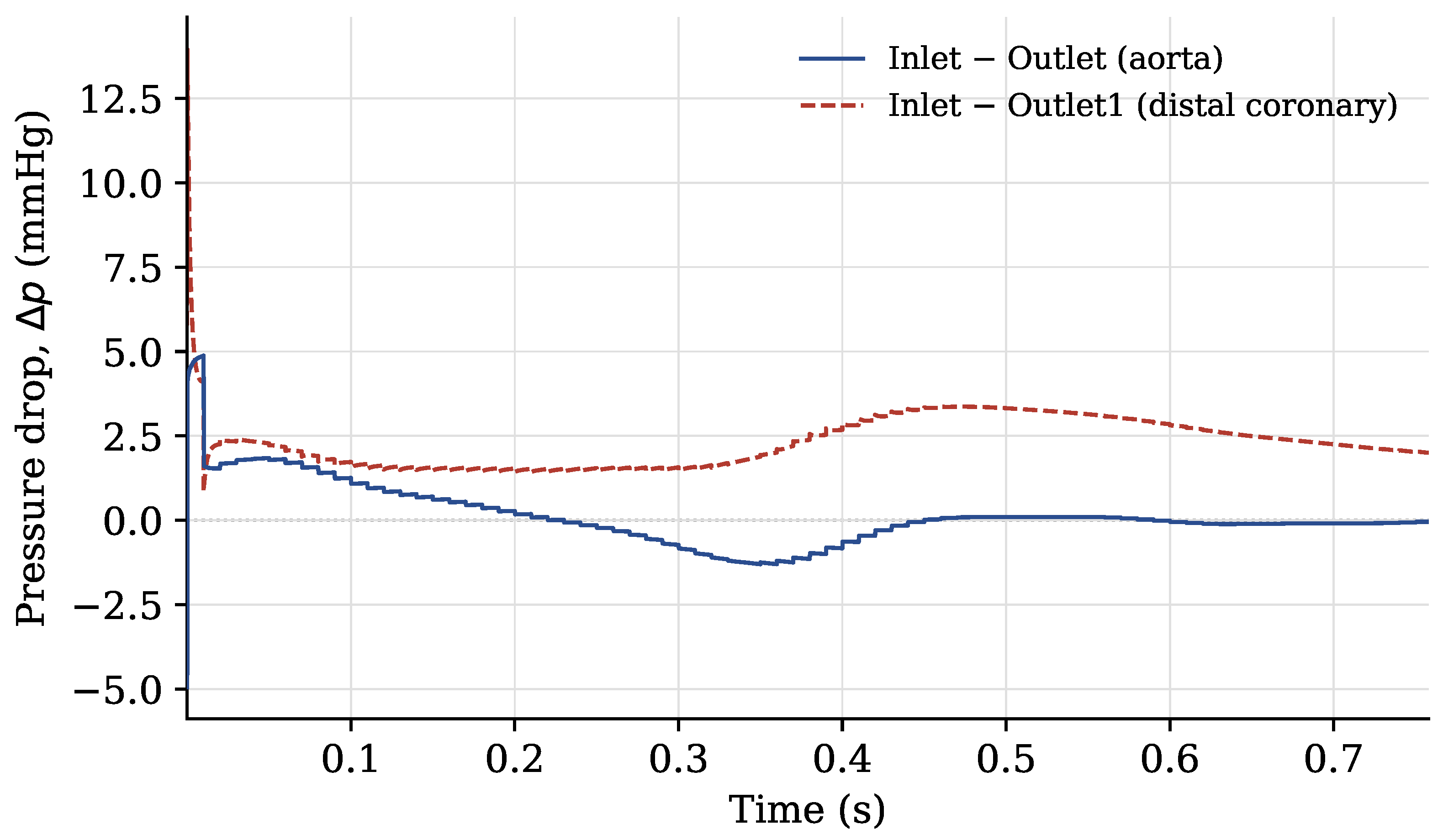
Along the aortic lumen, pressure variations are relatively small and change throughout the cardiac cycle as the flow accelerates and decelerates. By contrast, the coronary pathway exhibits a more persistent pressure reduction from the inlet towards the distal outlet. This difference reflects the distinct geometrical and haemodynamic characteristics of the two pathways: the aortic segment is short and has a relatively large calibre, whereas the coronary artery is longer, narrower, and more tortuous. To quantify these observations, Figure 16 reports the pressure differences between the inlet and the aortic and distal coronary outlets over the simulated cardiac cycle. The pressure drop was calculated as

$$\mathsf{\Delta }{p}_i\left(t\right)=p_{\mathrm{inlet}}\left(t\right)-p_{\mathrm{outlet},i}\left(t\right),$$

(27)

where the pressures are spatially averaged over the corresponding boundary patches.

Figure 16. Pressure differences between the inlet and the aortic and distal coronary outlets over the simulated cardiac cycle for case 1. The values are expressed in mmHg.

With the exception of the initial numerical transient, the pressure difference between the inlet and the aortic outlet remains close to zero throughout the cardiac cycle, with a mean value of approximately $0.07\mathrm{mmHg}$ and values ranging from $-1.3$ to $+4.4\mathrm{mmHg}$. Its sign reverses at several instants, indicating that the instantaneous pressure gradient along the aortic lumen changes direction during the pulsatile cycle. This behaviour is consistent with the response of a short, large-calibre, low-resistance vessel, in which viscous losses are limited and the local pressure gradient is strongly influenced by unsteady inertial effects. During flow acceleration and deceleration, the inertial contribution to the momentum balance may therefore produce a transient inversion of the pressure gradient. Such an inversion does not necessarily imply net retrograde flow through the aortic outlet. The amplitude of the aortic pressure oscillations, of the order of 1–$4\mathrm{mmHg}$, is also comparable to the dynamic-pressure scale

$$p_{\mathrm{dyn}}={\displaystyle \frac{1}{2}}\rho V^2.$$

(28)

For a characteristic peak velocity of $\mathcal{O}\left(1\mathrm{m}{\mathrm{s}}^{-1}\right)$ in the aortic segment and a blood density of $1060\mathrm{kg}{\mathrm{m}}^{-3}$, this expression gives a dynamic pressure of approximately $530\mathrm{Pa}$, corresponding to approximately $4.0\mathrm{mmHg}$. This comparison further indicates that the pressure variations along the aortic pathway are predominantly associated with pulsatile inertial effects rather than with irreversible viscous losses. In contrast, the pressure difference between the inlet and the distal coronary outlet remains positive throughout the cardiac cycle. Its mean value is approximately $2.4\mathrm{mmHg}$, with values ranging from $0.8$ to $3.6\mathrm{mmHg}$. The absence of a sign reversal indicates that a sustained pressure gradient is maintained from the inlet towards the distal coronary vasculature. This behaviour is consistent with the greater hydraulic resistance of the coronary pathway, arising from its smaller diameter, greater length, vessel curvature, and branching structure. Consequently, viscous effects play a more prominent role in the coronary arteries than in the large-calibre aortic segment.

4. Conclusions

A custom OpenFOAM solver was developed for the numerical simulation of patient-specific aortic–coronary haemodynamics. The framework combines a power-law inlet velocity profile selected according to the estimated Womersley regime, a three-element Windkessel condition at the aortic outlet, and dedicated lumped-parameter boundary conditions accounting for the downstream coronary circulation and intramyocardial pressure. The main outcomes of the study can be summarised as follows:

• The proposed framework provided stable coupling between the three-dimensional flow solver and the reduced-order outlet models in two patient-specific aortic-coronary geometries;
• The selected haemodynamic quantities showed limited sensitivity to further mesh refinement, with maximum local grid-convergence indices of $3.83\%$ for velocity magnitude and $2.21\%$ for pressure;
• The simulations reproduced pulsatile velocity and pressure fields, geometry-dependent recirculation patterns, and distinct pressure responses along the aortic and coronary pathways;
• The computed velocity and pressure magnitudes were comparable in scale with available in vivo measurements.

The proposed framework provides a basis for investigating local haemodynamics in patient-specific aortic–coronary anatomies while retaining the effects of the downstream vascular response. Future developments will focus on removing the rigid wall assumption, introducing FSI (fluid structure interaction), analysing wall shear stress-based indicators, performing a sensitivity analysis of the coronary outlet parameters, and the usage of further haemodynamic measurements.

References

- Herring, W. Capire la Radiologia: Le Basi Della Diagnostica per Immagini; Piccin: Padova, Italy, 2020; p. 408. [Google Scholar]
- Anastasi, G. Trattato di Anatomia Umana, 4th ed.; Edi-Ermes: Milano, Italy, 2006. [Google Scholar]
- Kim, H.J.; Vignon-Clementel, I.E.; Coogan, J.S.; Figueroa, C.A.; Jansen, K.E.; Taylor, C.A. Patient-Specific Modeling of Blood Flow and Pressure in Human Coronary Arteries. Ann. Biomed. Eng. 2010, 38, 3195–3209. [Google Scholar] [CrossRef] [Scilit] [PubMed]
- Sun, Z.; Xu, L. Computational fluid dynamics in coronary artery disease. Comput. Med. Imaging Graph. 2014, 38, 651–663. [Google Scholar] [CrossRef] [Scilit] [PubMed]
- Bottardi, A.; Prado, G.F.A.; Lunardi, M.; Fezzi, S.; Pesarini, G.; Tavella, D.; Scarsini, R.; Ribichini, F. Clinical Updates in Coronary Artery Disease: A Comprehensive Review. J. Clin. Med. 2024, 13, 4600. [Google Scholar] [CrossRef] [Scilit] [PubMed]
- Voges, I.; Jerosch-Herold, M.; Hedderich, J.; Pardun, E.; Hart, C.; Gabbert, D.D.; Kramer, H.; Rickers, C. Normal values of aortic dimensions, distensibility, and pulse wave velocity in children and young adults: A cross-sectional study. J. Cardiovasc. Magn. Reson. 2012, 14, 77. [Google Scholar] [CrossRef] [Scilit] [PubMed]
- Lamata, P.; Pitcher, A.; Krittian, S.; Nordsletten, D.; Bissell, M.M.; Cassar, T.; Barker, A.J.; Markl, M.; Neubauer, S.; Smith, N.P. Aortic relative pressure components derived from four-dimensional flow cardiovascular magnetic resonance. Magn. Reson. Med. 2014, 72, 1162–1169. [Google Scholar] [CrossRef] [Scilit] [PubMed]
- Yamaguchi, T.; Ishikawa, T.; Ichi Tsubota, K.; Imai, Y.; Nakamura, M.; Fukui, T. Computational Blood Flow Analysis—New Trends and Methods. J. Biomech. Sci. Eng. 2006, 1, 29–50. [Google Scholar] [CrossRef] [Scilit]
- Gijsen, F.J.H.; Wentzel, J.J.; Thury, A.; Mastik, F.; Schaar, J.A.; Schuurbiers, J.C.H.; Slager, C.J.; van der Giessen, W.J.; de Feyter, P.J.; van der Steen, A.F.W.; et al. Strain distribution over plaques in human coronary arteries relates to shear stress. Am. J. Physiol. Heart Circ. Physiol. 2008, 295, H1608–H1614. [Google Scholar] [CrossRef] [Scilit] [PubMed]
- Pandey, R.; Kumar, M.; Majdoubi, J.; Rahimi-Gorji, M.; Srivastav, V.K. A review study on blood in human coronary artery: Numerical approach. Comput. Methods Programs Biomed. 2019, 187, 105243. [Google Scholar] [CrossRef] [Scilit] [PubMed]
- Duronio, F.; Mascio, A.D. Blood Flow Simulation of Aneurysmatic and Sane Thoracic Aorta Using OpenFOAM CFD Software. Fluids 2023, 8, 272. [Google Scholar] [CrossRef] [Scilit]
- Cebral, J.R.; Castro, M.A.; Burgess, J.E.; Pergolizzi, R.S.; Sheridan, M.J.; Putman, C.M. Characterization of cerebral aneurysms for assessing risk of rupture by using patient-specific computational hemodynamics models. Am. J. Neuroradiol. 2005, 26, 2550–2559. [Google Scholar] [PubMed]
- Bockman, M.D.; Kansagra, A.P.; Shadden, S.C.; Wong, E.C.; Marsden, A.L. Fluid Mechanics of Mixing in the Vertebrobasilar System: Comparison of Simulation and MRI. Cardiovasc. Eng. Technol. 2012, 3, 450–461. [Google Scholar] [CrossRef] [Scilit]
- Boussel, L.; Rayz, V.; Martin, A.; Acevedo-Bolton, G.; Lawton, M.T.; Higashida, R.; Smith, W.S.; Young, W.L.; Saloner, D. Phase-Contrast MRI measurements in intra-cranial aneurysms in vivo of flow patterns, velocity fields, and wall shear stress: Comparison with CFD. Magn. Reson. Med. 2009, 61, 409–417. [Google Scholar] [CrossRef] [Scilit] [PubMed]
- Cai, S.; Mao, Z.; Wang, Z.; Yin, M.; Karniadakis, G.E. Physics-informed neural networks (PINNs) for fluid mechanics: A review. Acta Mech. Sin. 2021, 37, 1727–1738. [Google Scholar] [CrossRef] [Scilit]
- Caballero, A.D.; Laín, S. A Review on Computational Fluid Dynamics Modelling in Human Thoracic Aorta. Cardiovasc. Eng. Technol. 2013, 4, 103–130. [Google Scholar] [CrossRef] [Scilit]
- Etli, M.; Canbolat, G.; Karahan, O.; Koru, M. Numerical investigation of patient-specific thoracic aortic aneurysms and comparison with normal subject via computational fluid dynamics (CFD). Med. Biol. Eng. Comput. 2021, 59, 71–84. [Google Scholar] [CrossRef] [Scilit] [PubMed]
- DeVita, M.; Duronio, F.; Vita, A.D.; Berardinis, P.D. Adaptive Retrofit for Adaptive Reuse: Converting an Industrial Chimney into a Ventilation Duct to Improve Internal Comfort in a Historic Environment. Sustainability 2022, 14, 3360. [Google Scholar] [CrossRef] [Scilit]
- Dutta, H. Mathematical Methods in Engineering and Applied Sciences; Mathematics and Its Applications; CRC Press: Boca Raton, FL, USA, 2020. [Google Scholar]
- Duronio, F.; Mascio, A.D.; Villante, C.; Anatone, M.; Vita, A.D. ECN Spray G: Coupled Eulerian internal nozzle flow and Lagrangian spray simulation in flash boiling conditions. Int. J. Engine Res. 2023, 24, 1530–1544. [Google Scholar] [CrossRef] [Scilit]
- Berger, S.A.; Jou, L.D. Flows in Stenotic Vessels. Annu. Rev. Fluid Mech. 2000, 32, 347–382. [Google Scholar] [CrossRef] [Scilit]
- Pedley, T.J. The Fluid Mechanics of Large Blood Vessels; Cambridge University Press: Cambridge, UK, 1980. [Google Scholar] [CrossRef] [Scilit]
- Morris, L.; Delassus, P.; Callanan, A.; Walsh, M.; Wallis, F.; Grace, P.; McGloughlin, T. 3-D Numerical Simulation of Blood Flow through Models of the Human Aorta. J. Biomech. Eng. 2005, 127, 767–775. [Google Scholar] [CrossRef] [Scilit] [PubMed]
- Youssefi, P.; Gomez, A.; Arthurs, C.; Sharma, R.; Jahangiri, M.; Figueroa, C.A. Impact of Patient-Specific Inflow Velocity Profile on Hemodynamics of the Thoracic Aorta. J. Biomech. Eng. 2017, 140, 011002. [Google Scholar] [CrossRef] [Scilit]
- Qian, Y.; Liu, J.L.; Itatani, K.; Miyaji, K.; Umezu, M. Computational Hemodynamic Analysis in Congenital Heart Disease: Simulation of the Norwood Procedure. Ann. Biomed. Eng. 2010, 38, 2302–2313. [Google Scholar] [CrossRef] [Scilit] [PubMed]
- Zakaria, M.S.; Ismail, F.; Tamagawa, M.; Azi, A.F.A.; Wiriadidjaya, S.; Basri, A.A.; Ahmad, K.A. Computational Fluid Dynamics Study of Blood Flow in Aorta using OpenFOAM. J. Adv. Res. Fluid Mech. Therm. Sci. 2020, 43, 81–89. [Google Scholar]
- Boyd, J.; Buick, J.M. Comparison of Newtonian and Non-Newtonian Flows in a Two-Dimensional Carotid Artery Model Using the Lattice Boltzmann Method. Phys. Med. Biol. 2007, 52, 6215–6228. [Google Scholar] [CrossRef] [Scilit] [PubMed]
- Otani, T.; Nakamura, M.; Fujinaka, T.; Hirata, M.; Kuroda, J.; Shibano, K.; Wada, S. Computational Fluid Dynamics of Blood Flow in Coil-Embolized Aneurysms: Effect of Packing Density on Flow Stagnation in an Idealized Geometry. Med. Biol. Eng. Comput. 2013, 51, 901–910. [Google Scholar] [CrossRef] [Scilit] [PubMed]
- Wilson, N.M.; Ortiz, A.K.; Johnson, A.B. The Vascular Model Repository: A Public Resource of Medical Imaging Data and Blood Flow Simulation Results. J. Med. Devices 2013, 7, 0409231. [Google Scholar] [CrossRef] [Scilit]
- Safar, M.E.; Lévy, B.I. Resistance Vessels in Hypertension. In Comprehensive Hypertension; Lip, G.Y., Hall, J.E., Eds.; Mosby: Philadelphia, PA, USA, 2007; pp. 145–150. [Google Scholar] [CrossRef] [Scilit]
- Pochet, T.; Gerard, P.; Marnette, J.M.; D’Orio, V.; Marcelle, R.; Fatemi, M.; Fossion, A.; Juchmes, J. Identification of Three-Element Windkessel Model: Comparison of Time and Frequency Domain Techniques. Arch. Int. Physiol. Biochim. Biophys. 1992, 100, 295–301. [Google Scholar] [CrossRef] [Scilit] [PubMed]
- Tricarico, R.; Berceli, S.A.; Tran-Son-Tay, R.; He, Y. Non-Invasive Estimation of the Parameters of a Three-Element Windkessel Model of Aortic Arch Arteries in Patients Undergoing Thoracic Endovascular Aortic Repair. Front. Bioeng. Biotechnol. 2023, 11, 1127855. [Google Scholar] [CrossRef] [Scilit] [PubMed]
- Lungu, A.; Wild, J.; Capener, D.; Kiely, D.; Swift, A.; Hose, D. MRI Model-Based Non-Invasive Differential Diagnosis in Pulmonary Hypertension. J. Biomech. 2014, 47, 2941–2947. [Google Scholar] [CrossRef] [Scilit] [PubMed]
- Westerhof, N.; Lankhaar, J.W.; Westerhof, B.E. The Arterial Windkessel. Med. Biol. Eng. Comput. 2009, 47, 131–141. [Google Scholar] [CrossRef] [Scilit] [PubMed]
- Catanho, M.; Sinha, M.; Vijayan, V. Model of Aortic Blood Flow Using the Windkessel Effect; Technical Report; University of California: San Diego, CA, USA, 2012. [Google Scholar]
- Mantero, S.; Pietrabissa, R.; Fumero, R. The coronary bed and its role in the cardiovascular system: A review and an introductory single-branch model. J. Biomed. Eng. 1992, 14, 109–115. [Google Scholar] [CrossRef] [Scilit] [PubMed]
- Zhou, Y.; Kassab, G.S.; Molloi, S. On the design of the coronary arterial tree: A generalization of Murray’s law. Phys. Med. Biol. 1999, 44, 2929. [Google Scholar] [CrossRef] [Scilit] [PubMed]
- Sankaran, S.; Esmaily Moghadam, M.; Kahn, A.M.; Guccione, J.; Tseng, E.; Marsden, A.L. Patient-specific multiscale modeling of blood flow for coronary artery bypass graft surgery. Ann. Biomed. Eng. 2012, 40, 2228–2242. [Google Scholar] [CrossRef] [Scilit] [PubMed]
- Bittoni, F.; Dell’Agnello, F.; Duronio, F.; Degroote, J.; Di Mascio, A.; Battistoni, M. Comparison of Rigid-Wall Computational Fluid Dynamics and Flexible-Wall Fluid-Structure Interaction in Descending Thoracic Aorta Aneurysm. Fluids 2026, 11, 171. [Google Scholar] [CrossRef] [Scilit]
- Spalart, P.R.; Deck, S.; Shur, M.L.; Squires, K.D.; Strelets, M.K.; Travin, A. A New Version of Detached-Eddy Simulation, Resistant to Ambiguous Grid Densities. Theor. Comput. Fluid Dyn. 2006, 20, 181–195. [Google Scholar] [CrossRef] [Scilit]
- Angelo, L.D.; Duronio, F.; Vita, A.D.; Mascio, A.D. Cartesian Mesh Generation with Local Refinement for Immersed Boundary Approaches. J. Mar. Sci. Eng. 2021, 9, 572. [Google Scholar] [CrossRef] [Scilit]
- Roache, P.J. Quantification of uncertainty in computational fluid dynamics. Annu. Rev. Fluid Mech. 1997, 29, 123–160. [Google Scholar] [CrossRef] [Scilit]
- Duronio, F.; Di Mascio, A.; De Vita, A.; Innocenzi, V.; Prisciandaro, M. Eulerian–Lagrangian modeling of phase transition for application to cavitation-driven chemical processes. Phys. Fluids 2023, 35, 053305. [Google Scholar] [CrossRef] [Scilit]
- Di Mascio, A.; Dubbioso, G.; Muscari, R. Vortex structures in the wake of a marine propeller operating close to a free surface. J. Fluid Mech. 2022, 949, A33. [Google Scholar] [CrossRef] [Scilit]
- Pope, S.B.; Pope, S.B. Turbulent Flows; Cambridge University Press: Cambridge, UK, 2000. [Google Scholar]
- Ofili, E.O.; Kern, M.J.; St. Vrain, J.A.; Donohue, T.J.; Bach, R.G.; Al-Joundi, B.; Aguirre, F.V.; Castello, R.; Labovitz, A.J. Differential characterization of blood flow, velocity, and vascular resistance between proximal and distal normal epicardial human coronary arteries: Analysis by intracoronary Doppler spectral flow velocity. Am. Heart J. 1995, 130, 37–46. [Google Scholar] [CrossRef] [Scilit] [PubMed]
- Rigo, F.; Spadotto, V.; Fattore, R.S.; Renda, P.; Cugini, C.; Agnoletto, M. Normal physiologic coronary flow velocity gradient across the left anterior descending artery in healthy asymptomatic subjects. Explor. Cardiol. 2023, 1, 42–48. [Google Scholar] [CrossRef] [Scilit]
- Casadonte, L.; Verhoeff, B.J.; Piek, J.J.; VanBavel, E.; Spaan, J.A.E.; Siebes, M. Influence of increased heart rate and aortic pressure on resting indices of functional coronary stenosis severity. Basic Res. Cardiol. 2017, 112, 61. [Google Scholar] [CrossRef] [Scilit] [PubMed]
- Sakamoto, M.S.; Takahashi, M.S.; Coskun, P.A.; Papafaklis, M.M.; Takahashi, M.A.; Saito, M.S.; Stone, M.P.; Feldman, S.C. Relation of Distribution of Coronary Blood Flow Volume to Coronary Artery Dominance. Am. J. Cardiol. 2013, 111, 1420–1424. [Google Scholar] [CrossRef] [Scilit] [PubMed]
- Gallinoro, E.; Candreva, A.; Colaiori, I.; Kodeboina, M.; Fournier, S.; Nelis, O.; Di Gioia, G.; Sonck, J.; van ’t Veer, M.; Pijls, N.H.J.; et al. Thermodilution-derived volumetric resting coronary blood flow measurement in humans. EuroIntervention 2021, 17, e672. [Google Scholar] [CrossRef] [Scilit] [PubMed]
Disclaimer/Publisher’s Note: The statements, opinions and data contained in all publications are solely those of the individual author(s) and contributor(s) and not of MDPI and/or the editor(s). MDPI and/or the editor(s) disclaim responsibility for any injury to people or property resulting from any ideas, methods, instructions or products referred to in the content. |
© 2026 by the authors. Licensee MDPI, Basel, Switzerland. This article is an open access article distributed under the terms and conditions of the Creative Commons Attribution (CC BY) license.