Multi-Entity Balancing Responsibility Partitioning and Allocation for Micro-Dispatch Balancing Areas

Abstract

Micro-dispatch balancing areas need responsibility rules that distinguish deviation attribution from physically feasible corrective action. This study links a bus-level distance-based partitioning formulation with a constrained two-stage allocation model and quadratic Shapley attribution. Because the supplied network export and operating records are incomplete, the rebuilt case treats the six-area IEEE 118-bus partition as a fixed scenario and uses one 96-period proxy day containing 27 source profiles (four thermal and 23 renewable; 6916 MW). Under dimensionless objective scaling, the strict allocation is feasible within the modeled entity-level limits, requires neither external balancing nor cumulative slack, and assigns 9.71% of responsibility to thermal entities; exact quadratic Shapley attribution assigns 9.13%. For the co-directional set used here, normalized quadratic Shapley attribution is analytically identical to deviation-proportional allocation, so Monte Carlo differences measure sampling error rather than a distinct redistribution effect. Sensitivity tests show that the remaining constrained-versus-attribution gap depends on objective weights and obligation settings. Network-limit, partition-robustness, and seasonal-generalization claims are not made because the required inputs are unavailable.

1. Introduction

China’s generation mix is changing faster than the operating rules used to balance it. By the end of 2025, installed generation capacity had reached 3.89 billion kW, including approximately 1.20 billion kW of solar and 0.64 billion kW of wind capacity [1]. The operational consequence is straightforward: weather-driven output can move away from schedules within the trading day, while thermal units still carry much of the controllable balancing capability. A useful responsibility mechanism must therefore identify measurable deviations without assuming that every resource can respond in the same way.

The institutional setting already combines market and dispatch instruments. Day-ahead, intraday, and real-time transactions provide adjustment opportunities, while frequency regulation, reserves, and peak-shaving services provide additional flexibility [2,3]. Dispatch remains coordinated through unit commitment, automatic generation control, reserve management, interregional support, and emergency control under unified dispatch and hierarchical management [4]. The unresolved issue is not whether balancing exists, but how responsibility should be assigned within a smaller operating area when heterogeneous entities contribute differently to the observed deviation.

This question also appears in market settlement. Renewable energy communities must reconcile local transactions with wholesale balancing positions and flexibility commitments [5], while imbalance-fund allocation in China’s dual-track market links physical imbalance to participant revenues [6]. Across these settings, three requirements recur: the deviation must be measurable, the assigned responsibility must be traceable, and the allocation rule must remain compatible with operating and settlement constraints.

For a micro-dispatch area, a purely static rule is not enough. The allocation must close the regional imbalance, respect unit limits, distinguish the sign of the deviation, and account for regulation capability. Installed capacity or energy volume alone does not provide that information [7].

Existing allocation studies approach the problem from different directions. Weighting and mechanism-design methods derive obligations from policy targets or settlement behavior [6,7]; cooperative-game models distribute coordinated-dispatch gains or costs under uncertainty [8,9]; and virtual-power-plant studies combine market participation with Shapley-based allocation [10,11]. These strands are useful, but they solve different parts of the problem.

Hierarchical optimization addresses another part of the problem. Two-stage robust dispatch separates day-ahead and intraday decisions [9], while bilevel and iterative formulations model interactions among aggregators, internal resources, and market clearing [10,11]. Shapley variants have also been used to reflect forecast accuracy, environmental contribution, or member-specific value [10,11,12]. Most of these studies, however, start from a fixed aggregation boundary. They do not simultaneously define a responsibility area, enforce entity-level operating limits, and interpret the sources of the resulting imbalance.

The present study separates those functions instead of forcing them into one metric. Constrained optimization is used for operational allocation; quadratic Shapley analysis is used for attribution. For the coalition value adopted here, exact normalization over the co-directional participant set reduces to the deviation-proportional rule. We state that limiting result explicitly and use Monte Carlo sampling only to quantify approximation error, not as evidence of an additional optimization benefit.

Spatial partitioning supplies the missing boundary layer. Recent work combines grid structure with dynamic nodal characteristics rather than relying on administrative boundaries or operating convention [13]. Related studies have used graph-convolutional spectral clustering for electricity-market data [14], electrical-sensitivity information for virtual-power-plant control [15], and hierarchical coordination for wind-storage and multi-microgrid systems [16,17]. What remains less developed is a single workflow that links an electrically and temporally defined area to an allocation that respects operating limits and then to an attribution step that identifies each entity’s contribution. This paper examines that workflow from scheduled-versus-reference deviations.

This paper makes three contributions.

(1)

It formulates bus-level partitioning from normalized electrical and temporal-correlation distances, with K-means and graph spectral clustering as candidate boundary methods. The method requires complete network data and one aligned 96-period imbalance profile for every bus. Because those inputs are not available for the reconstructed case, the supplied six-area export is treated only as a fixed boundary; six areas and the original tuning parameters are not presented as empirically optimal or robust.

(2)

It uses one imbalance sign convention throughout and formulates a two-stage responsibility allocation that combines relative cost, baseline deviation, regulation capability, output bounds, ramp limits, and renewable regulation direction. The model separates strict feasibility from slack-assisted or relaxed variants rather than hiding infeasibility inside a penalty term.

(3)

It establishes the analytical relationship between quadratic Shapley attribution and co-directional deviation-proportional allocation. Exact attribution, Monte Carlo error, and constrained allocation are reported as different objects, all using the same participant registry and time grid.

The framework links the partitioning and allocation workflows. Section 3, Section 4 and Section 5 then distinguish the full proposed framework from the narrower numerical evidence that can be supported by the supplied data.

2. Mechanism of Entity Balancing Responsibility in Micro-Dispatch Balancing Areas

2.1. Definition and Design of the Micro-Dispatch Balancing Area

A micro-dispatch balancing area is treated here as an operating and accounting layer between local distribution resources and higher-level dispatch. Its boundary should follow metered tie points, network connectivity, resource distribution, and dispatch relationships rather than administrative geography alone. Once the boundary is fixed, the same area can be used to measure deviations, assign responsibility, and coordinate corrective action.

2.2. Imbalance Mechanism of the Micro-Dispatch Balancing Area

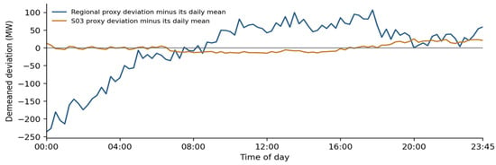
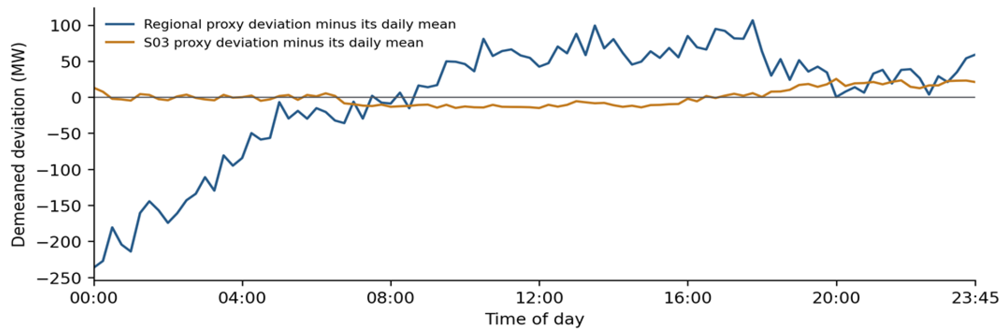
To isolate intraday shape from daily level, the fluctuation representation subtracts the daily mean from each regional or entity-level sequence. Figure 1 applies this centering to proxy deviations derived from the supplied available-power and clearing profiles. The notation below describes the general actual-output case; Section 5 states explicitly where the reconstructed dataset has a different interpretation.

$$q_{t,h,i,n}=P_{t,h,i,n}-P_{t,i,n}^{\mathit{mean}}$$

(1)

Figure 1. Demeaned regional and S03 proxy-deviation profiles in the rebuilt 27-entity case.

Here P denotes entity power, the superscript mean denotes the daily average, and q is the centered fluctuation. The subscripts identify day t, period h, entity i, and resource type n. The system-level expression is analogous:

$$q_{t,h}^{\mathit{sys}}=P_{t,h}^{\mathit{sys}}-P_t^{\mathit{sys},\mathit{mean}}$$

(2)

The superscript sys denotes the regional net-load sequence. Thus q measures departure from the daily mean; it is not a scheduled-versus-actual deviation.

This distinction matters for Figure 1. Parts of the centered curves fall below zero because the daily mean has been removed, even though every original proxy deviation in the rebuilt day is nonnegative. The figure therefore illustrates temporal shape, not cancellation between positive and negative generation deviations.

For this reason, an area boundary should reflect both network coupling and temporal behavior. Administrative location or resource type alone cannot capture either dimension.

2.3. Responsible Entities in a Micro-Dispatch Balancing Area

2.3.1. Thermal Power Entities

Institutional and Policy Basis

Thermal units enter the responsibility model because market and dispatch rules already impose generator obligations for transactions, dispatch instructions, effective capacity, and regulation services [2,3]. National regulation-capability programs also emphasize coal-unit flexibility and deep peak shaving [18]. Their balancing role is therefore operationally relevant, but it remains bounded by cost and unit constraints.

Physical Characteristics and Operating Mechanism

Thermal flexibility is not a single capability. Synchronous inertia and primary frequency response affect frequency security and reserve needs [19,20,21]; plant-side modifications such as bypass steam accumulators or sliding steam-temperature operation can change ramping performance [22,23]; and synchronous-condenser conversion can support voltage [24]. Measurement-based model validation and parameter identification provide additional evidence for performance assessment [25,26,27]. In the allocation model, these physical differences are condensed into minimum-output, ramping, availability, and relative-cost parameters. They are not treated as unlimited flexibility.

2.3.2. Renewable Energy Entities

Institutional and Policy Basis

Renewable resources are also moving toward explicit market responsibility. Current policy requires renewable electricity, in principle, to participate in market trading, either by submitting quantity and price bids or by accepting clearing prices [28]. This shift makes deviations relevant not only to system balancing but also to participant accounting.

Provincial rules add operational requirements: renewable plants or aggregations are expected to support forecasting, metering, and dispatch-instruction execution and to bear imbalance costs under the applicable market rules [29]. These requirements justify including renewable deviations in the same measurable responsibility framework used for conventional generation.

Physical Characteristics and Operating Mechanism

The difficulty is that renewable output is weather-dependent, intermittent, and non-stationary, so forecast error can cluster in particular periods [30,31,32]. Wind and solar capacity also continue to expand [33,34]. A responsibility rule should therefore reward better forecasting and controllability without assuming regulation capability that the plant does not have [35].

Accordingly, renewable responsibility is tied to measured deviation but bounded by available power, curtailment status, and regulation direction. An installed-capacity share is useful as a benchmark, not as a sufficient operational rule.

3. Partitioning of Micro-Dispatch Balancing Areas

3.1. Partitioning Framework

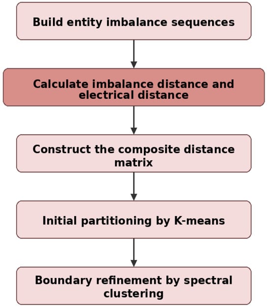
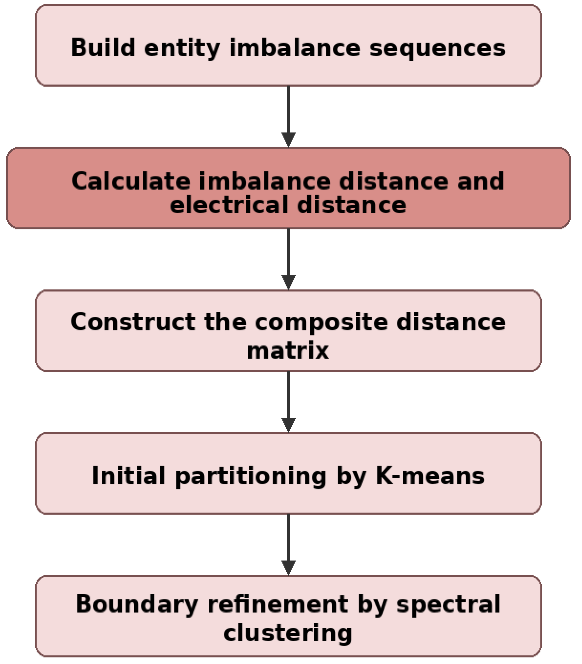
The partitioning formulation combines two signals: electrical coupling and similarity in temporal imbalance, as shown in Figure 2. Both distance matrices are normalized before weighting. K-means operates on the resulting distance features, while spectral clustering evaluates the same information as a sparse graph. The procedure can be tested only when complete network data and one aligned imbalance profile per bus are available. In Section 5, those inputs are incomplete, so the supplied partition is used as a fixed case-study boundary rather than re-created from missing data.

Figure 2. Framework for micro-dispatch balancing-area partitioning.

The resulting area is an operational accounting boundary, not a geographic district. Its purpose is to define which deviations are measured together and which entities participate in the same local balancing calculation.

3.2. Construction of Imbalance Features

Let scheduled (cleared) power and reference/actual power for entity i of type n in period h on day t be denoted as in Equation (3). Their difference defines the entity imbalance:

$$e_{t,h,i,n}=P_{t,h,i,n}^{\mathrm{act}}-P_{t,h,i,n}^{\mathrm{sch}}$$

(3)

A positive deviation means output above schedule; a negative value means a shortfall. In the surplus-only case used later, a positive responsibility is a downward correction, so the physical setpoint change has the opposite sign from the responsibility variable.

The total system imbalance is

$$E_{t,h}={\displaystyle {\displaystyle \sum }_{n=1}^3}{\displaystyle {\displaystyle \sum }_{i=1}^{I_n}}{e}_{t,h,i,n}$$

(4)

Here In is the number of entities of type n and Et,h is the net imbalance of the micro-dispatch area in period h.

At 15 min resolution, one day contains H = 96 periods. The entity sequence used for temporal comparison is

e_t,i,n = [e_t,1,i,n,e_t,2,i,n,…,e_t,H,i,n]

(5)

Because entities have different scales, each imbalance sequence is standardized before correlation is calculated:

$${\widehat{e}}_{i,h}={\displaystyle \frac{e_{i,h}-{\stackrel{-}{e}}_i}{{\sigma }_i+\epsilon }}$$

(6)

The mean and standard deviation are computed from the H observations for the same entity; ε only prevents division by zero.

The standardized sequence is then written as

$${\hat{e}}_{t,i,n}=\left[{\hat{e}}_{t,1,i,n},{\hat{e}}_{t,2,i,n},\dots ,{\hat{e}}_{t,H,i,n}\right]$$

(7)

3.3. Imbalance-Distance Calculation

Temporal similarity is measured by the correlation between the standardized entity sequences:

$$r_{\left(i,n\right),\left(j,m\right)}^{\mathrm{imb}}=\mathrm{corr}\left({\widehat{e}}_{t,i,n},{\widehat{e}}_{t,j,m}\right)$$

(8)

The correlation coefficient measures whether two standardized imbalance sequences move together. We convert it to a distance so that similar temporal patterns have small values:

$$d_{\left(i,n\right),\left(j,m\right)}^{\mathrm{imb}}=1-r_{\left(i,n\right),\left(j,m\right)}^{\mathrm{imb}}$$

(9)

This quantity is used only as the temporal component of the composite distance; it does not encode electrical proximity.

3.4. Electrical-Distance Calculation

Electrical distance is computed from the susceptance matrix rather than from geographic separation. Let B be the IEEE 118-bus susceptance matrix and B⁺ its Moore–Penrose pseudoinverse, with X = B⁺. The distance between buses a and b is

$$d_{a,b}^{\mathrm{ele}}=X_{\mathit{aa}}+X_{\mathit{bb}}-2X_{\mathit{ab}}$$

(10)

The bus indices in this expression must come from an explicit entity-to-bus registry. An entity number is not a bus number, and the two are never substituted for one another in the revised implementation.

Electrical and temporal distances are placed on a common numerical scale using min–max normalization:

$${\widehat{d}}_{a,b}={\displaystyle \frac{d_{a,b}-d_{\min }}{d_{\max }-d_{\min }+\epsilon }}$$

(11)

The extrema are taken from the corresponding distance matrix, with ε used only to avoid a zero denominator.

The normalized components are combined as

$$D_{a,b}={\lambda }_1{\widehat{d}}_{a,b}^{\mathrm{ele}}+{\lambda }_2{\widehat{d}}_{a,b}^{\mathrm{imb}}$$

(12)

λ₁ + λ₂ = 1

(13)

D_ij is the composite distance between indexed buses i and j. The weights λ₁ and λ₂ control the electrical and temporal contributions and satisfy λ₁ + λ₂ = 1.

3.5. K-Means and Spectral-Clustering Partitioning

Partitioning is performed at the bus level. Entity measurements must first be mapped or aggregated to buses through an explicit registry. Each row of D can then serve as a distance-feature vector for K-means. The 27 entity profiles in Section 5 are not copied across the 118 buses, and visualization coordinates are not used as substitutes for either distance matrix.

The distance-feature vector of bus i is defined as

$$z_i=\left[D_{i,1},D_{i,2},\dots ,D_{i,N_s}\right]$$

(14)

The vector z_i records the composite distance from bus i to every other indexed bus. It therefore preserves each bus’s position relative to the full network rather than compressing the comparison to one scalar feature.

For a candidate area count K, K-means partitions the indexed buses into disjoint sets C₁,…,C_k by minimizing within-cluster distance in this feature space:

$$\underset{C_k,{\mu }_k}{\min }{J}_{\mathrm{KM}}={\displaystyle {\displaystyle \sum }_{k=1}^K}{\displaystyle \sum }_{i\in C_k}{z}_i-{{\mu }_k}_2^2$$

(15)

$${\mu }_k={\displaystyle \frac{1}{\left|C_k\right|}}{\displaystyle \sum }_{i\in C_k}{z}_i,k=1,2,\dots ,K$$

(16)

Each iteration assigns bus i to the nearest cluster center:

$$c_i=\arg \underset{1\le k\le K}{\min }{z}_i-{{\mu }_k}_2^2$$

(17)

Here Ns is the number of indexed buses, Ck is area k, zi is the feature vector of bus i, and μk is its cluster center.

K is treated as a parameter, not fixed in advance by the algorithm. K-means provides one candidate partition, and spectral clustering provides a graph-based alternative whose quality must be judged from explicit metrics rather than assumed from the method name.

Boundary Refinement Based on Spectral Clustering

Spectral clustering first converts the composite distance into a sparse similarity graph, then embeds the buses using the normalized graph Laplacian. This representation can capture boundary structure that is not well described by Euclidean cluster centers, but any improvement must be demonstrated by the resulting metrics.

For a candidate neighborhood size k, an undirected edge is retained when either bus belongs to the other’s k-nearest-neighbor set. The corresponding similarity is

w_ij = exp[−D_ij²/(2σ²)] if j ∈ N_k(i) or i ∈ N_k(j); otherwise w_ij = 0, σ = s · median{D_ij | i < j}.

(18)

Nk(i) denotes the k-nearest-neighbor set of bus i. The dimensionless multiplier s scales the median positive composite distance, so k controls sparsity and s controls Gaussian-kernel width. Taking the union of the directed neighborhoods makes W symmetric.

The previously reported setting—(λ₁,λ₂) = (0.75, 0.25), k = 4, s = 0.45, and K = 6—is therefore treated as a candidate configuration, not a validated optimum. The reproducibility code prespecifies the requested grid over λ₁, k, s, and K, repeats each valid configuration over five random seeds, and reports silhouette, weighted modularity, normalized cut, graph-component count, label-aligned K-means-to-spectral changes, and adjusted Rand indices. The network part can be rebuilt from a declared MATPOWER case118 topology, but the 118 aligned temporal profiles and original preprocessing record are not available. We therefore provide the executable protocol without presenting unrun sensitivity results as evidence.

The degree matrix G is defined as

$$G_{\mathit{aa}}={\displaystyle {\displaystyle \sum }_{b=1}^{N_s}}{w}_{a,b}$$

(19)

The diagonal entries of G are the weighted degrees obtained by summing each row of W.

The normalized graph Laplacian is given by

L_sym = I − G^−1/2WG^−1/2

(20)

This normalized Laplacian is the matrix used for the spectral embedding.

The K eigenvectors corresponding to the smallest eigenvalues are selected:

L_symu_j = η_ju_j, j = 1, 2,…, K

(21)

These eigenvectors are arranged into matrix U. Each row is then normalized to obtain the corresponding bus representation in the spectral-embedding space:

$$Y_{\mathit{ij}}={\displaystyle \frac{U_{\mathit{ij}}}{\sqrt{{{\displaystyle \sum }}_{k=1}^K{U}_{\mathit{ik}}^2}}}$$

(22)

The selected eigenvectors form U; row normalization gives the embedding Y used for clustering.

K-means is subsequently applied in the spectral embedding space:

$$s_i=\arg \underset{1\le k\le K}{\min }{y}_i-{v_k}_2^2$$

(23)

Here yi is the embedded representation of bus i, vk is the kth center, and Ck is the assigned cluster. The resulting bus sets are

Ω_k = {i | s_i = k}, ⋃_k=1^K Ω_k = V, Ω_k ∩ Ω_l = ∅ (k ≠ l).

(24)

Ω_k is the set of buses assigned to micro-dispatch area k.

4. Reconstructed Allocation Model for the Surplus Case

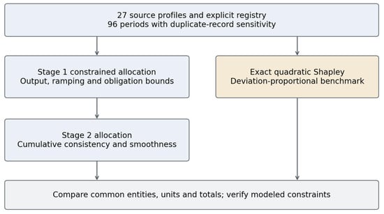
The allocation model is rebuilt directly from the 27 source columns, as shown in Figure 3 Renewable subtypes are pooled because the source fields do not distinguish wind from photovoltaic units. Operating limits and relative costs are stated scenario assumptions, and the imported partition is used only to define the participant boundary.

Figure 3. Computational workflow of the rebuilt 27-entity allocation example.

In an operational implementation, schedules would enter from the market-clearing system, while metered output, available-power estimates, and unit limits would come from dispatch telemetry such as SCADA/EMS. Corrective setpoints could then be issued through thermal AGC/governor interfaces and renewable plant controllers. The supplied files contain none of the device models, communication delays, protection settings, or closed-loop tests needed to validate that deployment path, so it is described only as an interface concept.

4.1. Proxy Deviation and Physical Adjustment

For the reconstructed case, Ahi is the supplied maximum-available-power reference, Chi the supplied clearing value, and Qi installed capacity. The source does not establish Ahi as metered actual generation or Chi as an observed market schedule. Every proxy deviation is nonnegative. Responsibility rhi is therefore modeled as a downward withdrawal of surplus, giving the adjusted output phi = Ahi − rhi. No deficit case is inferred from these data.

e_hi = A_hi − C_hi, E_h = Σ_i e_hi, p_hi = A_hi − r_hi

(25)

4.2. Baseline and First Stage

The first-stage baseline combines each entity’s deviation, share of available power, and share of installed capacity:

$$l_{\mathit{hi}}=0.50e_{\mathit{hi}}+0.20E_h{\displaystyle \frac{A_{\mathit{hi}}}{{\Sigma }_j A_{\mathit{hj}}}}+0.30E_h{\displaystyle \frac{Q_i}{{\Sigma }_j Q_j}}$$

(26)

The first-stage reference mixes three quantities: entity deviation, operating level, and capacity. For allocation r, define C = Σ_hic_ir_hi, D = Σ_hi|r_hi − l_hi|, and O = Σ_hi|r_hi − μ_ie_hi|/τ_i. We normalize these terms before weighting them:

$$F_1=\delta {\displaystyle \frac{C}{S_C}}+\theta {\displaystyle \frac{D}{S_D}}+\rho {\displaystyle \frac{O}{S_O}}$$

(27)

The scales are fixed from the same case: S_C = B max_ic_i, S_D = 2B, and S_O = B/min_iτ_i + Σ_hiμ_ie_hi/τ_i, where B = Σ_hE_h. These bounds place the objective terms on comparable dimensionless scales. The relative regulation coefficient c_i, obligation coefficient μ_i, and capability coefficient τ_i are also dimensionless in the rebuilt model. The weights δ, θ, and ρ sum to one.

4.3. Hard Operating Constraints

The balance, output, ramping, and obligation limits are:

$${\Sigma }_i r_{\mathit{hi}}+x_h=E_h,x_h\ge 0, 0\le r_{\mathit{hi}}\le A_{\mathit{hi}}-P_i^{\mathit{min}}$$

(28)

|p_hi − p_h−1,i|≤ R_i,r_hi ≥ μ_ie_hi

(29)

The variable x_h represents balancing supplied outside the selected entity set. It is minimized first; when the optimum is zero, x_h is fixed at zero before the remaining objective is optimized. Availability, minimum output, ramping, and responsibility-obligation constraints remain hard. Two thermal profiles are identically zero and are retained as entities but treated as unavailable, so both output and responsibility remain zero. Ramping is checked across the 95 within-day transitions because no preceding-day state or cyclic terminal condition is provided. Network flow is outside this entity-level formulation.

4.4. Second Stage and Cumulative Consistency

The second-stage objective adds a penalty for variation between adjacent periods:

$$F_2=\sigma {\displaystyle \frac{C}{S_C}}+\omega {\displaystyle \frac{D}{S_D}}+\phi {\displaystyle \frac{O}{S_O}}+\kappa {\displaystyle \frac{S}{S_S}}$$

(30)

In the second stage, D measures departure from the first-stage responsibility and S measures adjacent-period variation; C and O retain their first-stage definitions. S_S = 2B is used for the smoothness scale, leaving all four weighted terms dimensionless. For the cross-method comparison in Section 5.4, baseline deviation is evaluated against the same l for both the constrained and Shapley allocations. The weights σ, Ω, and φ sum to one, and κ controls smoothing. Each entity must also retain its first-stage daily total:

$${\Sigma }_h r_{\mathit{hi}}^2={\Sigma }_h r_{\mathit{hi}}^1 \left(i=1,\dots ,27\right)$$

(31)

The main specification enforces cumulative consistency exactly. A soft variant introduces positive and negative cumulative-gap variables and minimizes their sum after external balancing but before the second-stage objective. A third variant removes cumulative consistency altogether. No hidden obligation slack is added. Because the observed proxy day contains only surplus deviations, both stages already represent downward action; the second-stage tests therefore isolate cumulative consistency and temporal smoothing. Absolute-value terms are linearized and solved with SciPy 1.17.0 using HiGHS.

4.5. Exact Shapley Attribution and Baselines

For each period, the coalition value is the square of its members’ total deviation:

$$v\left(S\right)={({\Sigma }_{i\in S}{e}_{\mathit{hi}})}^2,{\phi }_{\mathit{hi}}=e_{\mathit{hi}}{E}_h$$

(32)

For the quadratic coalition game, entity i’s expected marginal contribution is e_hi² + e_hiΣ_j ≠ _ie_hj. In a mixed-sign game, raw Shapley values can be negative and carry units of MW². Over the co-directional set, however, a_i = |e_hi| and A⁺ = Σa_i imply φ_i = a_iA⁺. Normalization therefore yields

$$r_{\mathit{hi}}^{\mathit{Sh}}=\left|E_h\right|{\displaystyle \frac{a_i}{A^{+}}}=r_{\mathit{hi}}^{\mathit{dev}}$$

(33)

The normalized quadratic rule is thus exactly the same as the co-directional deviation-proportional baseline. In this all-positive case, both reduce to e_hi. We also evaluate a capacity-proportional rule and a deviation-proportional rule. The raw capacity rule is additionally repaired by a minimum-L1 adjustment under the same availability, minimum-output, and ramping constraints; that repair does not impose the optimizer-specific μ obligation, which is reported separately. Monte Carlo error is measured against the exact Shapley solution using 20 independent seeds.

5. Rebuilt 27-Entity Case Study

5.1. Fixed Partition and Entity Boundary

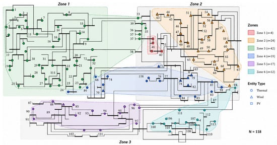
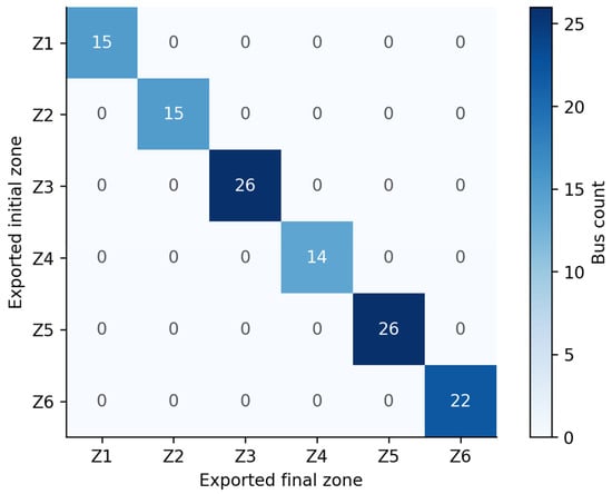
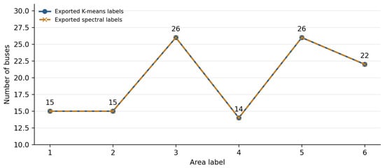
The supplied IEEE 118-bus topology partition is retained in Figure 4 because it provides the spatial context for the reconstructed case. We treat this topology as an audited fixed boundary, not as a reproduced clustering result. The K-means and final-label columns both contain zone sizes of 15, 15, 26, 14, 26, and 22 buses, and row-wise comparison gives zero bus-label changes. Figure 5 and Figure 6 audit the exported label transition and zone counts; neither establishes that spectral clustering improved the partition.

Figure 4. Supplied IEEE 118-bus micro-dispatch balancing-area partition retained as the spatial reference for the reconstructed case. (The topology figure is preserved from the original manuscript; clustering was not rerun, and the numbers represent node identifiers).

Figure 5. Transition matrix between the exported initial and final partitions. All 118 bus labels are unchanged.

Figure 6. Exported bus counts by area before and after the reported refinement. (The overlapping lines reflect identical supplied labels; the plot does not represent an independently rerun sensitivity study.).

The export contains four useful fields—Bus, KmeansZone, SpectralZone, and two plotting coordinates—but none of the matrices or time series needed to reconstruct the reported clustering. In particular, it lacks the electrical-distance matrix, temporal-distance matrix, sparse similarity graph, and one 96-period imbalance profile for each bus. The uploaded partition script can rebuild an electrical distance from MATPOWER case118, but it cyclically maps spreadsheet rows to buses and uses MDS plus K-means rather than the reported sparse-graph spectral procedure. A corrected implementation now requires explicit bus identifiers and can reconstruct the network distance, yet it still cannot manufacture the missing temporal profiles. We therefore remove the former 15- and 26-label-change claims, do not report silhouette/modularity/normalized-cut values that were never computed, and treat the six-area partition as an imported scenario rather than evidence of robust parameter tuning.

Zone 5 contains 26 buses: 68, 76–98, 116, and 118. The 27 source entities are assigned to these buses through a declared experimental mapping: S01–S26 follow the ordered bus list and S27 shares bus 118 with S26. This mapping is not an observed Jiangsu connection record. It is used only to keep bus membership and entity counting explicit; because no network-flow constraints are included, it cannot establish an electrical advantage for this partition.

5.2. Dataset and Parameter Definition

The participant registry in Table 1 contains four thermal entities (S01–S04) and 23 renewable entities (S05–S27), with installed capacities of 1360 MW and 5556 MW, respectively; total capacity is 6916 MW. The source fields do not support a defensible wind/PV split, so the renewable group is left unclassified. S02 and S04 remain in the registry even though their reference profiles are zero throughout the day.

Table 1. Complete registry for the reconstructed Zone 5 example. All bus connections are constructed.

Entity	Bus	Type	Capacity (MW)
S01	68	Thermal	330.00
S02	76	Thermal	330.00
S03	77	Thermal	350.00
S04	78	Thermal	350.00
S05	79	Renewable	149.10
S06	80	Renewable	153.60
S07	81	Renewable	157.30
S08	82	Renewable	315.00
S09	83	Renewable	152.00
S10	84	Renewable	200.00
S11	85	Renewable	302.00
S12	86	Renewable	400.00
S13	87	Renewable	400.00
S14	88	Renewable	350.00
S15	89	Renewable	150.00
S16	90	Renewable	400.00
S17	91	Renewable	300.00
S18	92	Renewable	150.00
S19	93	Renewable	200.00
S20	94	Renewable	300.00
S21	95	Renewable	50.00
S22	96	Renewable	48.00
S23	97	Renewable	100.00
S24	98	Renewable	279.00
S25	116	Renewable	300.00
S26	118	Renewable	400.00
S27	118	Renewable	300.00

Rows containing capacity and maximum-output metadata are removed from the time series. Both source tables contain a duplicated 23:45 record. The main case keeps the first occurrence and the sensitivity case keeps the second; neither is asserted to be the verified observation. The source date and provenance of the clearing values are also unavailable. The reproducibility files therefore retain original row numbers, source columns, capacities, and the declared bus mapping.

The operating limits and relative costs in Table 2 are scenario assumptions, not recovered plant parameters. The reported cost index, 0.25Σc_ir_hi, is measured in relative-cost-weighted MWh and should not be read as currency. We also remove the former photovoltaic coefficient μ_PV = 0.25/RMSE from the rebuilt case. If RMSE is expressed in MW, that expression makes μ dimensioned in MW⁻¹ and μe dimensionless; if normalized RMSE was intended, the normalization basis, time window, and PV entity labels are missing. The pooled renewable group therefore uses an explicit dimensionless coefficient, with μ_R tested from 0.25 to 0.75 in the sensitivity analysis.

Table 2. Declared parameters of the reconstructed example.

Parameter	Thermal	Renewable
Obligation coefficient μ	1.00	0.50
Capability coefficient τ	0.25	0.05
Relative cost c	1.00	0.20
Online minimum output	0.20 Q	0
Ramp limit per 15 min	0.25 Q	1.00 Q
Baseline weights	0.50, 0.20, 0.30	same
Stage 1 and 2 weights	0.33, 0.34, 0.33	same
Smoothness κ	0.10	same

5.3. Recomputed Constrained Allocation

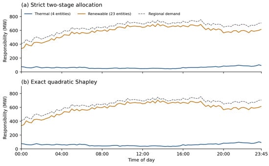
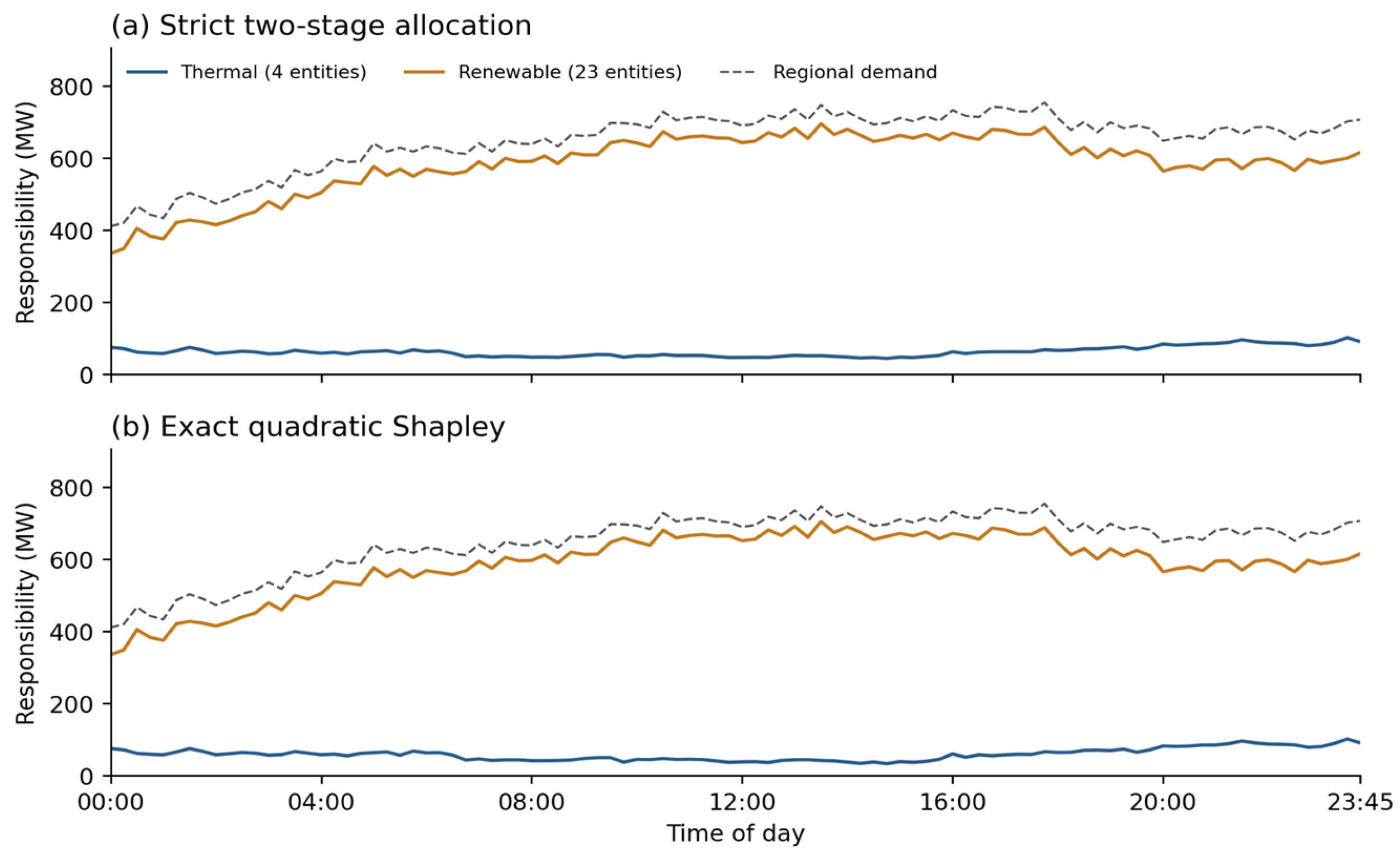
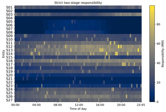
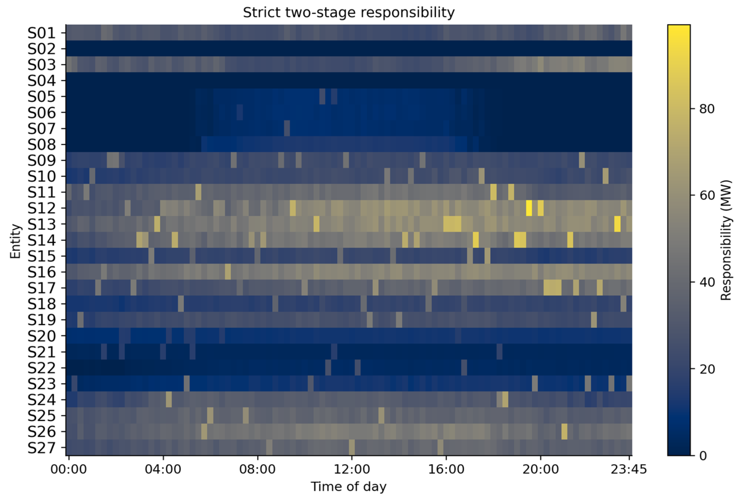
The 96-period proxy day has a mean balancing demand of 647.45 MW and a peak of 754.07 MW. Cumulative demand is 62,155.42 MW-periods, equivalent to 15,538.86 MWh at 15 min resolution. Under the strict two-stage model, thermal entities receive 9.71% of responsibility and renewables 90.29%; exact quadratic Shapley attribution gives thermal entities 9.13%. Figure 7 shows the type totals and Figure 8 the final entity-by-period allocation.

Figure 7. Thermal and renewable responsibility profiles under the strict two-stage and exact Shapley rules.

Figure 8. Recomputed responsibility heatmap for all 27 entities under the strict two-stage model.

The strict solution closes the modeled balance without external resources. Its maximum balance residual is 2.27 × 10⁻¹³ MW; output and ramping violations remain below the 10⁻⁷ MW reporting tolerance. No entity exceeds a cumulative gap of 10⁻⁶ MW-periods, and the largest numerical cumulative residual is 2.73 × 10⁻¹² MW-periods. Strict, minimum-slack, and no-cumulative-consistency variants therefore collapse to the same allocation at numerical precision (Table 3).

Table 3. Recomputed cumulative-consistency comparisons under the default parameters.

Second-Stage Setting	External (MWh)	Total |Gap| (MW-Periods)	Gap/Demand (%)	Active Entities
Strict	0.000	1.60 × 10−11	2.58 × 10−14	0
Minimum slack	0.000	1.60 × 10−11	2.58 × 10−14	0
No cumulative constraint	0.000	1.71 × 10−13	2.74 × 10−16	0

We define the slack ratio as 100Σ_i|Σ_hr²_hi − Σ_hr¹_hi|/Σ_hE_h. In both the strict and minimum-slack runs, the ratio is 2.58 × 10⁻¹⁴%, which is solver roundoff; under the 10⁻⁶ MW-period reporting threshold, activated slack is zero. Removing cumulative consistency also leaves the default allocation unchanged. The previously reported 17,850.94 MW-periods cannot be traced to a reproducible optimizer and participant set, so it is withdrawn rather than reinterpreted. At κ = 0.10, the largest first-to-second-stage change is 1.90 × 10⁻¹² MW. Thus the default case demonstrates feasibility, not additional smoothing. This statement applies only to the modeled entity limits; network-flow feasibility has not been established.

5.4. Allocation Rules and Shapley Analysis

5.4.1. Constrained Allocation Versus Attribution

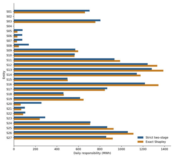
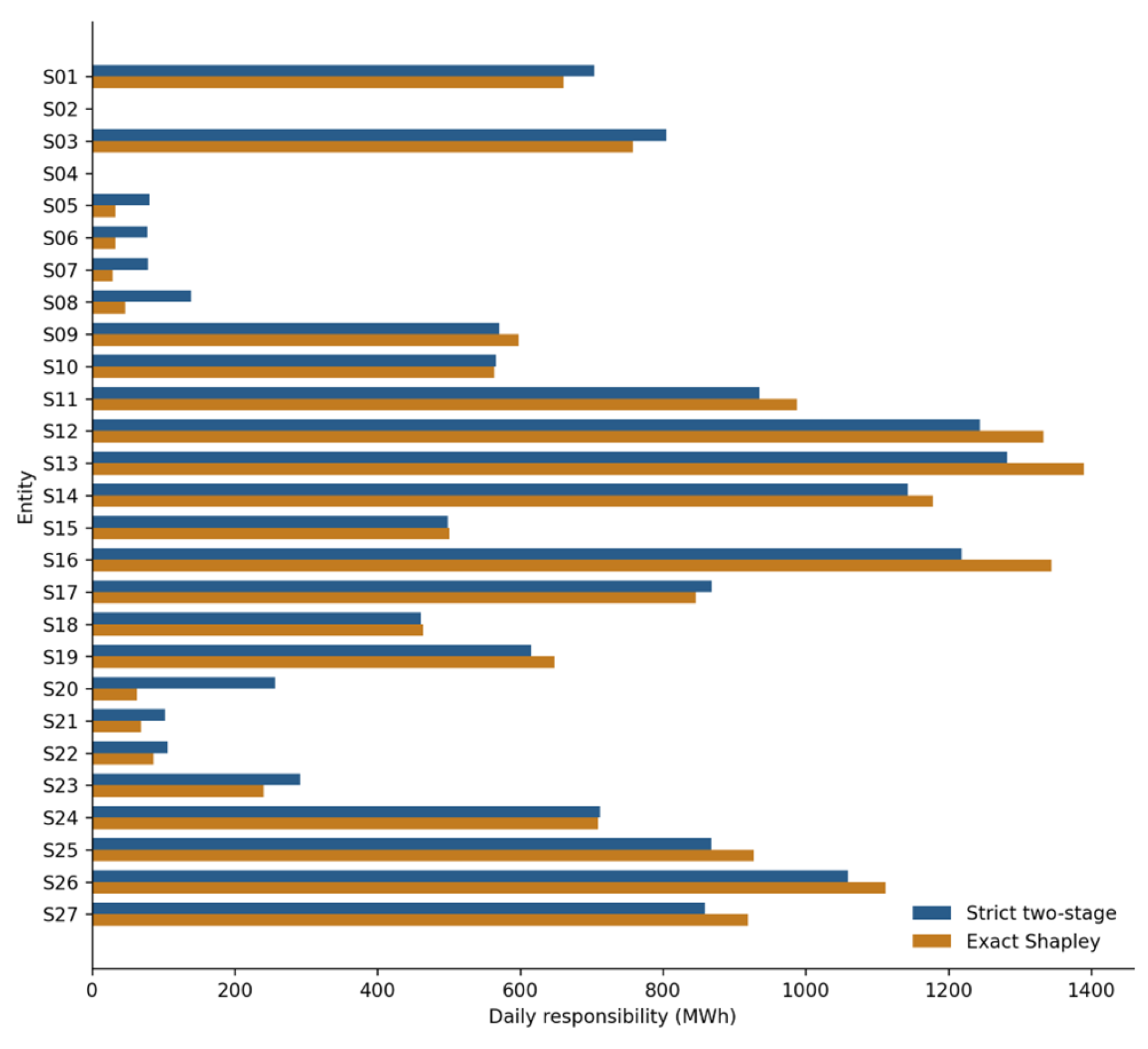
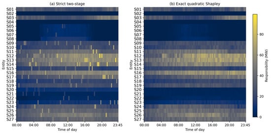
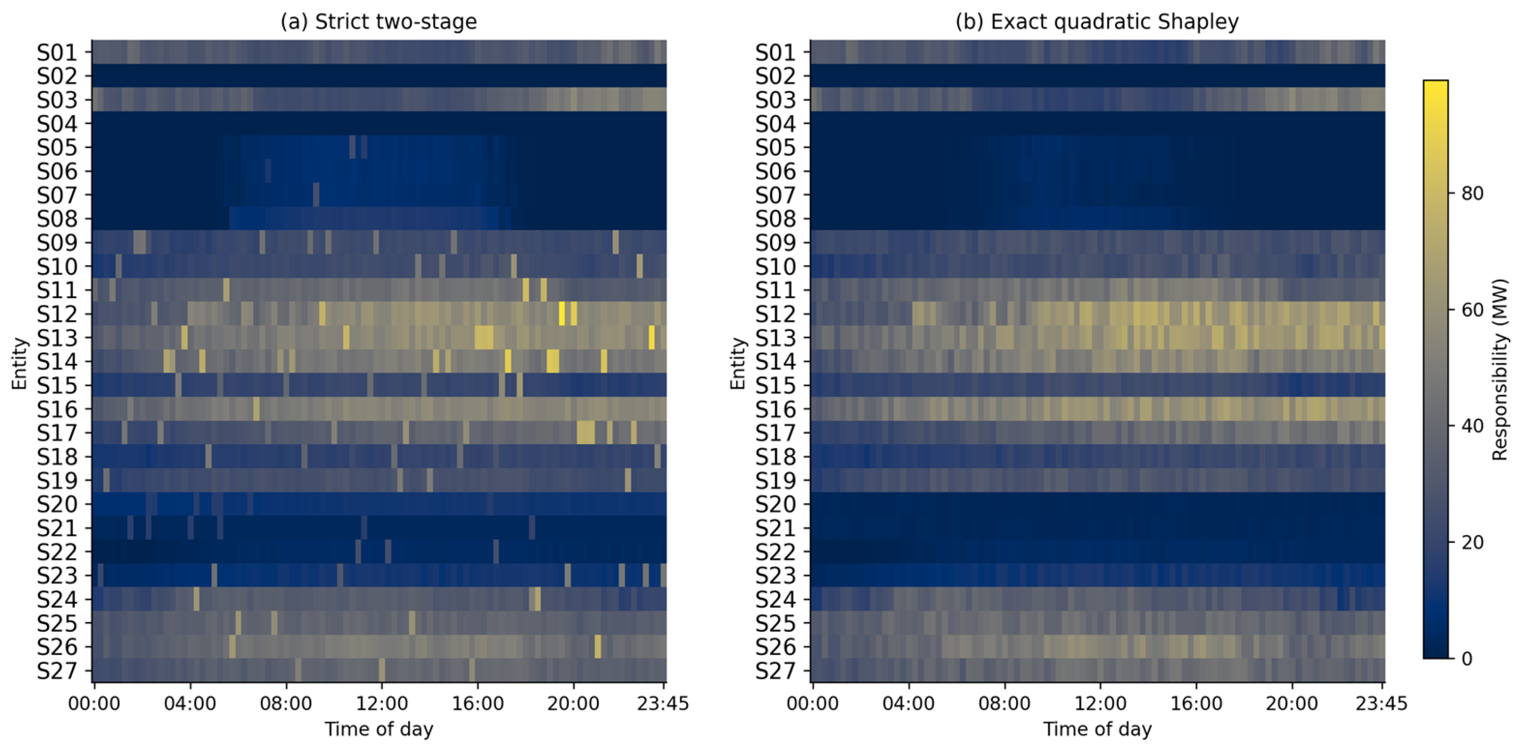
Figure 9 and Figure 10 compare the constrained allocation and exact Shapley attribution using the same 27 entities and time grid. The mean absolute pointwise difference is 3.49 MW and the maximum is 43.25 MW. The thermal shares are 9.71% and 9.13%, respectively—a difference of 0.58 percentage points. Under the stated parameters, the constrained model therefore assigns slightly more responsibility to thermal entities than the attribution rule.

Figure 9. Daily responsibility of all 27 entities under constrained allocation and exact Shapley attribution.

Figure 10. Recomputed responsibility heatmaps on a common scale for constrained allocation and exact Shapley attribution. (Panels (a,b) show the strict two-stage allocation and exact quadratic Shapley attribution, respectively; rows identify S01–S27, columns are 15 min periods, and the shared color scale is in MW).

That gap is far smaller than the earlier unscaled comparison. What remains reflects the combined effect of the baseline, relative-cost coefficients, obligation settings, and hard operating constraints. It should not be interpreted as evidence that thermal entities caused more of the underlying source deviation. Table 4 compares cost, fairness, and entity-level feasibility.

Table 4. Cost, fairness and feasibility comparison for the same 27 entities and 96 periods.

Method	Thermal (%)	Cost Index	Cost Δ (%)	Jain Cap.	Capacity Align.	Deviation Align.	Violating Cells
Constrained two-stage	9.71	4314.32	+0.00	0.790	0.768	0.927	0
Capacity pro rata raw	19.66	5552.29	+28.69	1.000	1.000	0.733	602
Capacity pro rata repaired	10.48	4410.53	+2.23	0.833	0.813	0.753	0
Deviation pro rata	9.13	4242.82	−1.66	0.730	0.733	1.000	0
Exact quadratic Shapley	9.13	4242.82	−1.66	0.730	0.733	1.000	0

No single fairness metric is treated as definitive. We report three transparent diagnostics: a capacity-normalized Jain index based on daily responsibility per MW of installed capacity, alignment with the capacity-proportional reference, and alignment with the deviation-proportional reference. The two alignment scores are one minus total-variation distance, so a value of one means exact agreement with the stated rule. The cost index is the relative-cost-weighted energy 0.25Σ_hic_ir_hi; because c_i is an assumed relative coefficient, this is not a monetary operating cost.

The raw capacity rule is perfectly capacity proportional, but under the assumed coefficients its cost index is 28.69% above the constrained solution and it violates unit-level limits in 602 entity-period cells; the largest lower-bound violation is 38.16 MW. A minimum-L1 repair removes those physical violations but leaves a 660.59 MW-period obligation deficit. The deviation rule is exactly deviation proportional and has a cost index 1.66% below the constrained solution in this scenario. It also satisfies the tested entity-level bounds but does not preserve the optimizer’s first-stage entity totals. These comparisons expose competing reference principles; they do not establish a universal ranking of fairness.

Using the same dimensionless diagnostic, as shown in Table 5, the constrained allocation scores 0.21476 and exact Shapley scores 0.22466. The −0.00990 difference decomposes exactly into cost (+0.00152), baseline deviation (−0.01183), obligation (−0.00103), and smoothness (+0.00144). This accounting explains the diagnostic-score gap only; it is not an additive causal decomposition of the thermal-share difference. Table 6 reports the effect of removing each objective term.

Table 5. Dimensionless objective-component comparison under the reported weights.

Method	Cost	Baseline Deviation	Obligation	Smoothness	Total
Constrained	0.09162	0.01575	0.10078	0.00661	0.21476
Exact Shapley	0.09011	0.02758	0.10182	0.00516	0.22466
Difference	0.00152	−0.01183	−0.00103	0.00144	−0.00990

Table 6. Objective-term ablation under the first-record dataset.

Model	Thermal (%)	Gap from Shapley (pp)	Variation (MW)
Full model	9.7059	+0.5752	8211.63
Remove cost term	13.9663	+4.8355	5782.81
Remove baseline-deviation term	9.1307	+0.0000	3601.95
Remove obligation term	9.7059	+0.5752	8210.38
Remove smoothness term	9.7059	+0.5752	8211.63

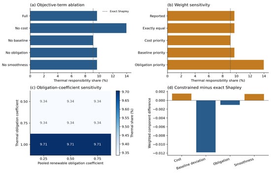
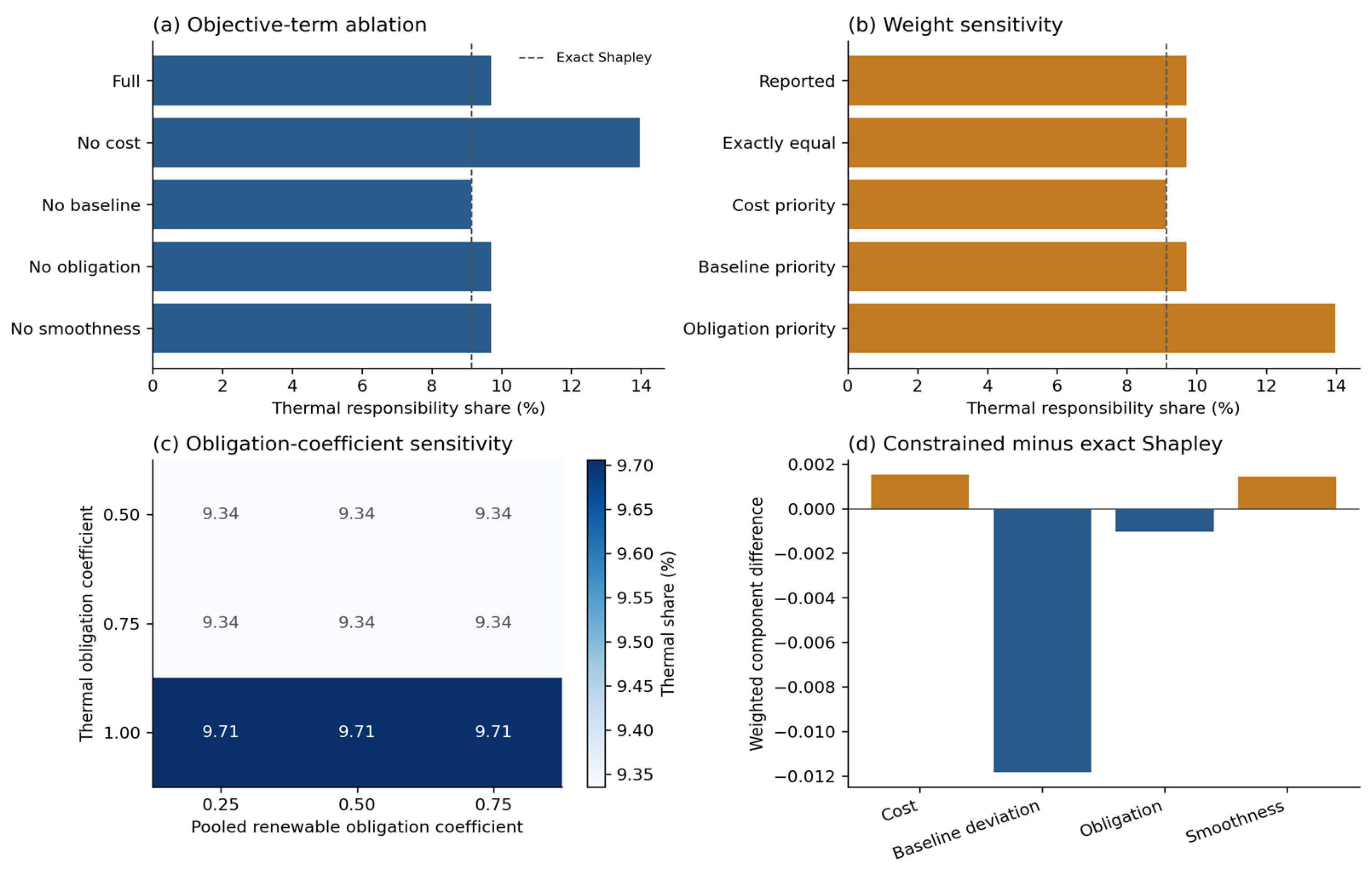
The tests in which individual terms are removed support this distinction. Removing baseline deviation moves the thermal share to 9.1307%, matching exact Shapley in this case, whereas removing the cost term raises it to 13.9663%. Dropping the obligation term from the objective does not change the share because the obligation inequality remains a hard constraint. Removing smoothness also leaves daily shares unchanged because the second stage preserves cumulative entity totals. Since these effects interact through the constraints, they are reported separately rather than summed as independent causes. Figure 11 summarizes these tests, parameter sensitivity, and the weighted component differences.

Figure 11. Objective-term ablation, objective-weight sensitivity, obligation-coefficient sensitivity and weighted component differences.

5.4.2. Analytical Equivalence and Monte Carlo Error

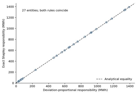
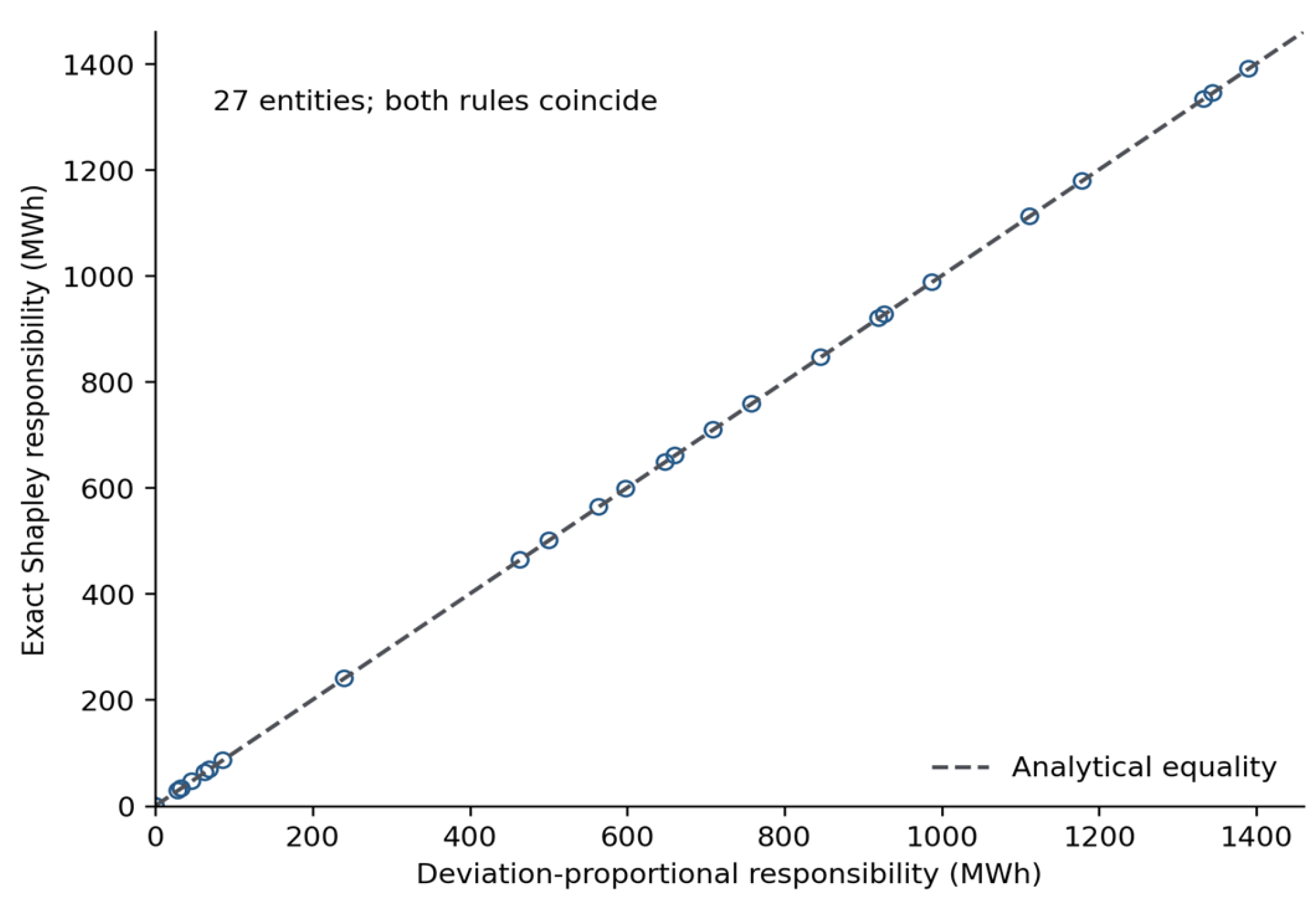
Equation (33) shows that, after normalization, the quadratic Shapley second layer is identical to the co-directional deviation-proportional first layer. Figure 12 verifies this result for all 27 daily totals; the largest pointwise difference is 2.84 × 10⁻¹⁴ MW. The exact two-layer construction therefore introduces no substantive redistribution. Any discrepancy produced by finite random permutations is sampling error.

Figure 12. Exact equality of deviation-proportional and normalized quadratic Shapley daily responsibilities.

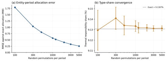
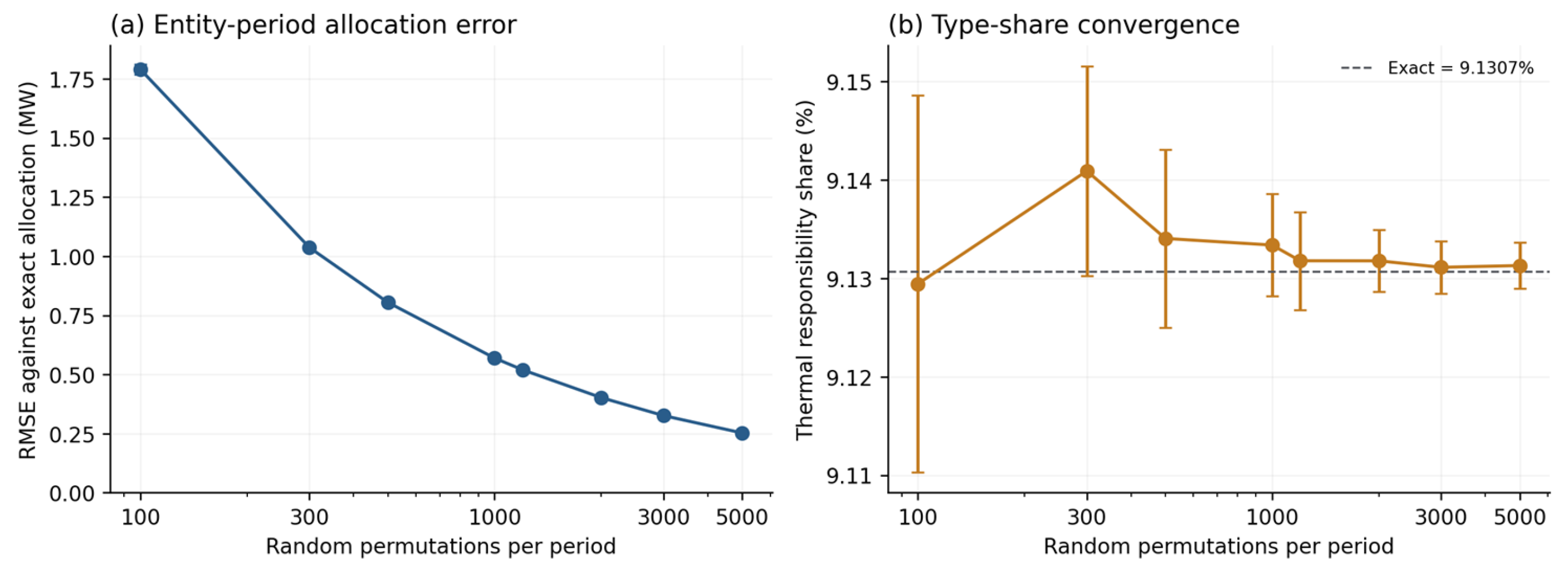
We quantify that error over 20 independent seeds at M = 100, 300, 500, 1000, 1200, 2000, 3000, and 5000 permutations per period. Figure 13 shows 95% confidence intervals, calculated with Student’s t distribution, for the mean across the 20 seeds. Mean RMSE is 0.5693 MW at M = 1000 (95% CI 0.5630–0.5757), 0.5196 MW at M = 1200 (0.5143–0.5249), and 0.2527 MW at M = 5000 (0.2498–0.2556). The exact thermal share is 9.1307%; at M = 1200 the mean estimate is 9.1318% with a 95% CI of 9.1268–9.1368%. These intervals describe Monte Carlo variability only, not uncertainty across operating days.

Figure 13. Monte Carlo convergence against the exact quadratic allocation. (Error bars show 95% confidence intervals for the means across the seeds from 20 independent seeds).

5.5. Duplicate Record and Parameter Sensitivity

Using the second 23:45 record instead of the first lowers cumulative demand to 62,130.26 MW-periods (15,532.56 MWh). The constrained thermal share becomes 9.6963% and the exact Shapley share 9.1180%. Both variants remain feasible under the stated entity constraints. This check quantifies sensitivity to the duplicate record; it does not identify which record is historically correct. Table 7 and Table 8 report sensitivity to objective weights and obligation coefficients, respectively.

Table 7. Sensitivity to cost, baseline-deviation and obligation weights.

Weights (Cost, Baseline, Obligation)	Thermal (%)	Gap from Shapley (pp)	Variation (MW)
(0.33, 0.34, 0.33)	9.7059	+0.5752	8211.63
(1/3, 1/3, 1/3)	9.7059	+0.5752	8211.63
(0.60, 0.20, 0.20)	9.1307	+0.0000	7230.20
(0.20, 0.60, 0.20)	9.7059	+0.5752	8211.63
(0.20, 0.20, 0.60)	13.9663	+4.8355	3900.85

Table 8. Thermal responsibility share under dimensionless obligation coefficients.

Thermal μ	Renewable μ = 0.25	Renewable μ = 0.50	Renewable μ = 0.75
0.50	9.3353%	9.3353%	9.3353%
0.75	9.3353%	9.3353%	9.3353%
1.00	9.7059%	9.7059%	9.7059%

The reported weight triple (0.33,0.34,0.33) and the exactly equal triple produce the same thermal share, 9.7059%. Across the tested emphasis cases, the share spans 9.1307–13.9663%; across the obligation grid it spans 9.3353–9.7059%. Varying the pooled renewable coefficient changes the temporal allocation but not the daily thermal total within this grid, while increasing the thermal coefficient from 0.75 to 1.00 raises that total. Increasing κ to 0.50 reduces responsibility variation to 1985.95 MW, 75.82% below the default, while cumulative entity totals remain fixed. The earlier large model-versus-Shapley contrast is therefore not a stable structural property; it was sensitive to scaling and parameter choice.

5.6. Network and Cross-Scenario Evidence Audit

We added an ex-post DC line-flow verifier, but the supplied evidence does not satisfy its input gate. In the declared MATPOWER case, all 186 in-service branches have zero or missing RATE_A limits. The entity-to-bus mapping is constructed rather than verified, and a complete 118-bus post-allocation injection table is unavailable. Any line-loading percentage would therefore depend on invented limits or injections. The verifier returns BLOCKED and will run the 96-period check only when positive limits, verified connections, and balanced full-network injections are supplied.

The same constraint applies to geographical and seasonal generalization. Only one zone has usable entity data, and the date and season of the proxy day are unspecified. Relabeling or scaling that day would create synthetic stress tests, not independent evidence for other areas or seasons. The reproducibility package therefore includes a machine-readable manifest and templates for the missing cases rather than fabricated multi-zone results. Table 9 summarizes the missing evidence and the inputs required for each check.

Table 9. Status of the requested network and generalization evidence.

Requested Evidence	Available Evidence	Status	Required to Complete
Ex post line-limit verification	186 branches; 0 positive limits	BLOCKED	Positive limits, verified mapping and 118-bus injections
Additional zones	1 zone (Z5)	BLOCKED	At least two additional verified zones
Seasonal days	Season/date unspecified	BLOCKED	Spring, summer, autumn and winter 96-period days

5.7. Scope of the Recomputed Evidence

Every numerical comparison in the rebuilt study uses the same 27-entity registry. The evidence is limited to one surplus-only proxy day, a pooled renewable category, and a constructed bus placement. Complete 118-bus time series are absent for the partition sweep, and verified line ratings, connections, and full-network injections are absent for power-flow validation. The revised manuscript therefore makes no claim of an optimal six-area partition, network security, seasonal robustness, or monetary cost savings. Fifteen targeted tests cover the source population, a known LP optimum, infeasibility reporting, setpoint feasibility, exact Shapley enumeration, objective scaling and component identities, reference-rule metrics, baseline violations, duplicate handling, partition/mapping identity, deterministic sweep calculations, invalid-profile rejection, the MATLAB(R2025b) sweep interface, and the network-evidence gate.

6. Conclusions

The reconstructed study resolves the participant-definition problem by using one 27-entity registry—four thermal and 23 renewable entities totaling 6916 MW—across every allocation and attribution calculation. All rules use the same 96-period time grid. The supplied six-area IEEE 118-bus file is retained only as a fixed boundary; its two exported label columns are identical, so the available evidence does not demonstrate spectral-clustering improvement or robustness to distance weights, neighborhood size, kernel scale, or area count. The declared bus mapping is experimental and is not presented as a recovered connection record.

Within that explicitly limited surplus case, the strict constrained allocation is feasible under the modeled entity-level bounds, uses no external balancing, and activates no cumulative slack above the reporting tolerance. After dimensionless objective scaling, thermal entities receive 9.71% of responsibility, compared with 9.13% under deviation-based attribution. The 0.58-percentage-point gap changes under objective ablation and weight sensitivity. The default second stage does not alter the first-stage solution, although stronger smoothing can reduce temporal variation while preserving cumulative entity totals. The constrained allocation also does not dominate the deviation-proportional baseline on every reported metric.

The Shapley analysis has a narrower interpretation than originally claimed. Exact quadratic normalization over a co-directional set reproduces deviation-proportional allocation, so the two-layer construction is an analytical consistency check rather than an independent improvement mechanism. Monte Carlo error decreases with sample size and should be reported as estimator uncertainty, not redistribution benefit. Stronger empirical claims require dated schedules, verified resource subtypes and connections, complete network inputs, positive line ratings, and operating scenarios that include both surplus and deficit deviations.

References

- National Energy Administration. 2025 National Power Statistics Released by the National Energy Administration. Available online: https://www.nea.gov.cn/20260129/6874f211acd0417eab7ac10c3061a7c2/c.html (accessed on 29 January 2026).
- National Development and Reform Commission; National Energy Administration. Basic Rules for the Electricity Spot Market (Trial); NDRC Energy Regulation No. 1217. 2023. Available online: https://www.gov.cn/zhengce/zhengceku/202309/content_6904881.htm (accessed on 1 August 2026).
- National Development and Reform Commission; National Energy Administration. Basic Rules for the Electricity Ancillary Service Market; NDRC Energy Regulation No. 411. 2025. Available online: https://www.gov.cn/zhengce/zhengceku/202505/content_7022228.htm (accessed on 1 August 2026).
- National Development and Reform Commission; National Energy Administration. Measures for Interprovincial and Interregional Emergency Power Dispatch Management; NDRC Operation Regulation No. 1193. 2025. Available online: https://www.ndrc.gov.cn/xxgk/zcfb/ghxwj/202510/t20251013_1400912.html (accessed on 1 August 2026).
- Mello, J.; Villar, J. Integrating flexibility and energy local markets with wholesale balancing responsibilities in the context of renewable energy communities. Energy 2023, 282, 128853. [Google Scholar] [CrossRef] [Scilit]
- Long, S.; Wu, Z.; Li, H.; Xu, J.; Yue, Z.; Cheng, X. Imbalance funds allocation mechanism design in China’s dual track electricity market environment: An agent-based modeling approach. Energy Strategy Rev. 2024, 52, 101344. [Google Scholar] [CrossRef] [Scilit]
- Tang, Y.; Liu, Y.; Huo, W.; Chen, M.; Ye, S.; Cheng, L. Optimal allocation scheme of renewable energy consumption responsibility weight under renewable portfolio standards. Energies 2023, 16, 3085. [Google Scholar] [CrossRef] [Scilit]
- Song, D.; Xue, T.; Li, Y.; Tu, J.; Bi, Y.; Wang, M. Cooperative game scheduling and revenue sharing strategy for virtual power plants considering scenery uncertainty. Electr. Power Eng. Technol. 2025, 44, 193–206. [Google Scholar] [CrossRef]
- Ju, L.; Lv, S.; Zhang, Z.; Li, G.; Gan, W.; Fang, J. Data-driven two-stage robust optimization dispatching model and benefit allocation strategy for a novel virtual power plant considering carbon-green certificate equivalence conversion mechanism. Appl. Energy 2024, 362, 122974. [Google Scholar] [CrossRef] [Scilit]
- Liu, R.; Chen, K.; Sun, G.; Lin, S.; Jiang, C. Bidding strategy for the virtual power plant based on cooperative game participating in the electricity-carbon joint market. Int. J. Electr. Power Energy Syst. 2024, 163, 110325. [Google Scholar] [CrossRef] [Scilit]
- Shang, Y.; Li, X.; Xu, T.; Cui, L. Uncertainty-output virtual power plant participates in multi-electricity market considering the improved Shapley value distribution method. Int. J. Electr. Power Energy Syst. 2025, 165, 110462. [Google Scholar] [CrossRef] [Scilit]
- Zhang, S.; Pang, L.; Li, Y.; Chen, Y.; Li, K.; Zheng, M. Green-fitting scheduling equilibrium model of virtual power plant based on cooperative game with improved Shapley value under new-type power system. Int. J. Electr. Power Energy Syst. 2025, 168, 110704. [Google Scholar] [CrossRef] [Scilit]
- Yang, A.; Yang, M.; Xie, L.; Shao, J. Two-stage voltage control partitioning method for distribution network containing distributed generation. Electr. Power Eng. Technol. 2025, 44, 219–227. [Google Scholar]
- Huang, L.; Shan, M.; Weng, L.; Meng, L. Graph convolutional spectral clustering for electricity market data clustering. Appl. Sci. 2024, 14, 5263. [Google Scholar] [CrossRef] [Scilit]
- Hyun, S.; Kim, G.; Park, J.; Choi, Y. Optimal virtual power plant control algorithm considering the electrical characteristics of distributed energy resources. Appl. Sci. 2025, 15, 127. [Google Scholar] [CrossRef] [Scilit]
- Nan, J.; Feng, J.; Guan, L.; Sun, K.; Deng, X.; Zhou, H. A two-stage Stackelberg game wind-storage planning model considering a bus carbon intensity incentive mechanism. Appl. Sci. 2023, 13, 3710. [Google Scholar] [CrossRef] [Scilit]
- Zhang, J.; Xuan, W.; Yang, D.; Lyu, G.; Guan, Y. Co-scheduling strategies for intra-microgrid dual demand response and inter-microgrid P2P cooperation. Electr. Power Eng. Technol. 2025, 44, 103–113. [Google Scholar]
- National Development and Reform Commission; National Energy Administration. Implementation Plan for the Special Action on Optimizing Power System Regulation Capability (2025–2027); NDRC Energy No. 1803. 2024. Available online: https://www.gov.cn/zhengce/zhengceku/202501/content_6996643.htm (accessed on 1 August 2026).
- Zhou, J.; Guo, Y.; Yang, L.; Shi, J.; Zhang, Y.; Li, Y.; Guo, Q.; Sun, H. A review on frequency management for low-inertia power systems: From inertia and fast frequency response perspectives. Electr. Power Syst. Res. 2024, 228, 110095. [Google Scholar] [CrossRef] [Scilit]
- Ullmark, J.; Göransson, L.; Johnsson, F. Frequency reserves and inertia in the transition to future electricity systems. Energy Syst. 2024, 15, 1527–1560. [Google Scholar] [CrossRef] [Scilit]
- Zhou, L.; Wang, H.; Wang, Y.; Zhang, H.; Li, W.; Li, R. Evaluation of the impact of inertia on system operation cost. Front. Energy Res. 2023, 11, 1118349. [Google Scholar] [CrossRef] [Scilit]
- Ding, H.; Ding, S.; Tan, Q.; Zhang, C. Improving power ramp rate of a coal-fired power plant by a bypass steam accumulator. Heliyon 2024, 10, e32412. [Google Scholar] [CrossRef] [Scilit]
- Wang, P.; Wang, C.; Xiao, Q.; Huang, C.; Liu, M.; Chen, W.; Yan, J. Enhancing the ramp-up flexibility of the coal-fired power plant under deep peak shaving work conditions by adopting a sliding steam temperature scheme. Energy 2025, 335, 137864. [Google Scholar] [CrossRef] [Scilit]
- Liu, M.; Tian, C.; Yuan, X.; Li, C.; Gao, Z.; Zhang, D. The influence of stability in new power systems with the addition of phase modulation functions in thermal power units. Processes 2024, 12, 2897. [Google Scholar] [CrossRef] [Scilit]
- Hong, F.; Ji, W.; Pang, Y.; Hao, J.; Du, M.; Fang, F.; Liu, J. A new energy state-based modeling and performance assessment method for primary frequency control of thermal power plants. Energy 2023, 276, 127594. [Google Scholar] [CrossRef] [Scilit]
- Gholamnejad, S.; Delkhosh, H.; Seifi, H. Performance evaluation of power plants in primary frequency control integrating heuristic parameter extraction optimization and share attribution mechanism. Int. J. Electr. Power Energy Syst. 2025, 172, 111183. [Google Scholar] [CrossRef] [Scilit]
- Chen, X.; Jiang, Y.; Terzija, V.; Lu, C. Review on measurement-based frequency dynamics monitoring and analyzing in renewable energy dominated power systems. Int. J. Electr. Power Energy Syst. 2024, 155, 109520. [Google Scholar] [CrossRef] [Scilit]
- National Development and Reform Commission; National Energy Administration. Notice on Deepening Market-Oriented Reform of Renewable On-Grid Electricity Prices and Promoting High-Quality Renewable Development; NDRC Price No. 136. 2025. Available online: https://www.ndrc.gov.cn/xwdt/tzgg/202502/t20250209_1396067.html (accessed on 1 August 2026).
- Shandong Office of the National Energy Administration; Shandong Development and Reform Commission; Shandong Energy Administration. Shandong Electricity Market Rules (Trial). 2025. Available online: https://sdb.nea.gov.cn/dtyw/tzgg/202512/t20251217_292527.html (accessed on 1 August 2026).
- Zhang, L.; He, F.; Chen, M.; He, C.; Huang, Z.; Wang, C.; Yan, L. An adaptive early warning method for wind power prediction error. Processes 2025, 13, 3941. [Google Scholar] [CrossRef] [Scilit]
- Duan, W.; Zhang, Z.; Zhong, A.; Tang, Z. A robust wind power forecasting framework for non-stationary signals via decomposition and metaheuristic optimization. Energies 2025, 18, 6515. [Google Scholar] [CrossRef] [Scilit]
- Wu, G.; Hu, D.; Zhang, Y.; Bao, G.; He, T. A convolutional neural network-long short-term memory-attention solar photovoltaic power prediction-correction model based on the division of twenty-four solar terms. Energies 2024, 17, 5549. [Google Scholar] [CrossRef] [Scilit]
- National Energy Administration. 2024 National Power Industry Statistics Released by the National Energy Administration. Available online: https://www.nea.gov.cn/20250121/097bfd7c1cd3498897639857d86d5dac/c.html (accessed on 21 January 2025).
- National Energy Administration. Grid-Connected Operation of Renewable Energy in 2024. Available online: https://www.nea.gov.cn/20250221/e10f363cabe3458aaf78ba4558970054/c.html (accessed on 21 February 2025).
- Yu, H.; Lee, J.; Wi, Y.-M. Day-ahead PV generation scheduling in incentive program for accurate renewable forecasting. Appl. Sci. 2024, 14, 228. [Google Scholar] [CrossRef] [Scilit]
Disclaimer/Publisher’s Note: The statements, opinions and data contained in all publications are solely those of the individual author(s) and contributor(s) and not of MDPI and/or the editor(s). MDPI and/or the editor(s) disclaim responsibility for any injury to people or property resulting from any ideas, methods, instructions or products referred to in the content. |
© 2026 by the authors. Licensee MDPI, Basel, Switzerland. This article is an open access article distributed under the terms and conditions of the Creative Commons Attribution (CC BY) license.