


Featured Application
A weibit-based combined distribution and assignment model and a fast partial linearization solution algorithm that can be applied in network-level travel-demand forecasting for transportation planning.
Abstract
The combined distribution and assignment (CDA) problem is considered in which both the destination choice and the route choice follow the multinomial weibit model rather than the conventional multinomial logit model. Existing CDA models typically adopt a hierarchical logit structure with independently and identically distributed Gumbel errors, whose fixed perception variance is unrealistic when trips of very different lengths are handled simultaneously. To circumvent this drawback, a hierarchical weibit choice structure is developed in which the perceived travel costs follow the Weibull distribution, making the perception variance route-specific and increasing with the trip length, and a weibit composite cost plays the role of the logsum in the logit-based CDA model. An equivalent mathematical programming formulation is constructed by combining a multiplicative Beckmann transformation with route-level and destination-level entropy terms, an exogenous destination utility term, and a path-size term, and its equivalence and uniqueness are proved. An equivalent variational inequality formulation accommodates further model extensions. A path-based partial linearization algorithm is developed whose search direction is obtained in closed form by the hierarchical weibit loading and whose step size follows Barzilai–Borwein strategies, including an adaptive scheme. Numerical experiments on the Winnipeg network demonstrate the computational performance of the algorithm and the behavioral differences from the logit-based model. A validation against the observed Winnipeg demand further shows that, once both models are calibrated to the observed mean trip length, the weibit-based model reproduces the observed demand pattern substantially more closely than its logit counterpart.
1. Introduction
Travel-demand forecasting has traditionally been carried out by the sequential four-step procedure: trip generation, trip distribution, modal split, and traffic assignment. A well-known deficiency of the sequential procedure is the internal inconsistency of the level of service (or travel cost) variables among the steps [1]. Combined travel-demand models were developed to resolve this inconsistency by determining the travel choices of interest simultaneously within a single mathematical structure, such that a mutually consistent set of flows and costs is obtained at equilibrium [2,3,4,5,6].
Among the various combined models, the combined distribution and assignment (CDA) model, which integrates the destination choice and the route choice, has received considerable attention because of its wide applicability in transportation systems analysis. Among others, CDA models have been used (1) as the lower-level subprogram of network design problems in which the land-use distribution and network layout jointly determine the travel-demand pattern [7,8]; (2) in the analysis of network capacity, capacity reliability, and capacity flexibility, where the destination choice serves as a demand-adjustment mechanism under capacity limitations [9,10,11]; and (3) in taxi operation modeling, where the simultaneous movements of vacant and occupied taxis are described by a CDA structure [12,13]. More recent applications of combined destination and route type equilibrium structures include the capacity analysis of multimodal networks with emerging travel modes [14], park-and-ride facility location [15], and shared parking services [16].
In terms of behavioral foundation, the state-of-the-practice CDA model is the hierarchical logit choice model based on random utility theory [5]. Each traveler at origin first chooses a destination s according to a multinomial logit (MNL) model defined on the expected received disutility of all routes between origin and destination (O-D), and then chooses a route according to an MNL model defined on the route travel costs. This hierarchical logit structure admits an elegant equivalent mathematical programming (MP) formulation of the entropy type, in which the Beckmann transformation is combined with two entropy terms associated with route choice and destination choice [3,5,17]. The entropy-type structure is also the key to the development of efficient solution algorithms, notably the classical partial linearization algorithm and, more recently, dual approaches for side-constrained versions [17,18].
However, the logit-based CDA model inherits the well-known drawbacks of the MNL model rooted in the independently and identically distributed (IID) Gumbel assumption on the random error terms [19]: (1) the independence assumption implies an inability to account for the overlapping (or correlation) among routes; and (2) the identically distributed assumption implies an identical, fixed perception variance with respect to trips of different lengths over all routes and all O-D pairs. The second drawback is particularly troublesome in the CDA context. In a combined model, trips of very different lengths are handled simultaneously not only across O-D pairs but also across destinations within the same origin since the destination choice explicitly compares near and far destinations. A choice model whose perception variance is insensitive to the overall trip length distorts both levels of the hierarchy. It produces route-choice probabilities based solely on absolute cost differences regardless of the overall trip length, and it propagates this distortion upward into the destination choice through the logsum. Although the scaling technique of Chen et al. [20], which replaces the single dispersion parameter with individual O-D-specific dispersion parameters, can partially relax the identically distributed assumption at the O-D level, it cannot distinguish the perception variances of individual routes within the same O-D pair.
Castillo et al. [21] proposed the multinomial weibit (MNW) model as a route-choice model without the identically distributed assumption. By assuming that the perceived route travel costs follow the Weibull distribution rather than the conventional Gumbel distribution, the MNW model has a simple analytical probability expression with route-specific perception variances that increase with the route travel cost. Kitthamkesorn and Chen [22] subsequently provided an equivalent MP formulation for the MNW stochastic user equilibrium (SUE) problem by developing a multiplicative Beckmann’s transformation combined with an entropy term, and introduced a path-size factor to obtain the path-size weibit (PSW) model that simultaneously handles the route overlapping and route-specific perception variance problems. Follow-up studies have extended the weibit modeling framework in several directions, including the unconstrained formulation [23], the unified logit-weibit representation [24], comparative analyses of logit and weibit route choices [25], hybrid absolute relative cost models [26], semiparametric generalizations [27,28], positive location parameters [29], systematic property analyses [30], the paired combinatorial weibit model [31], and multiplicative regret-based equilibria [32]. The weibit framework has also begun to extend into combined travel choice modeling. Kitthamkesorn et al. [33] applied the path-size weibit SUE model with elastic demand to the combined modal split and traffic assignment problem. Kitthamkesorn et al. [34] and Kitthamkesorn and Chen [35] developed weibit-based combined mode and route-choice models for assessing green transport systems and, most recently, Gu et al. [16] proposed a weibit-based combined destination and parking choice equilibrium model for shared parking services. Nevertheless, the classical combined distribution and assignment problem has not yet been addressed within the weibit framework, with the combined destination and parking choice model of Gu et al. [16] being the closest development to date. Existing CDA models with a random utility foundation, from the hierarchical logit CDA [5,17] to its extended logit variants [36], remain logit-based.
Motivated by the above observations, the objective of this paper is to develop a weibit-based CDA (WCDA) model in which both the destination choice and the route choice are governed by the weibit model in a hierarchical structure. The contributions of this paper are fourfold:
- Modeling: We develop a hierarchical weibit choice structure for the CDA problem. A weibit composite cost, defined as the scale parameter of the minimum perceived route travel cost distribution between an O-D pair and available in closed form because of the closure of the Weibull distribution under minimization, is identified as the natural weibit counterpart of the logsum and serves as the level-of-service feedback variable from the route-choice level to the destination-choice level.
- Formulation: We provide an equivalent MP formulation for the WCDA model by combining the multiplicative Beckmann’s transformation with two entropy terms (route-level and destination-level) and a rescaled shape parameter, in direct analogy to the logit-based CDA formulation. The equivalence and uniqueness properties are rigorously proved. We also provide an equivalent VI formulation for model extensions in which the route travel cost is not decomposable at the link level.
- Solution algorithm: We develop a path-based partial linearization algorithm in the spirit of Evans [3] for solving the WCDA model. Because the entropy terms are retained in the subproblem, the search direction is obtained analytically by applying the hierarchical weibit probabilities (destination choice and route choice) to the current cost pattern. The step size is determined by Barzilai–Borwein (BB) step-size strategies (BB1 and BB2) recently shown to outperform monotone averaging schemes in path-based SUE computation [37], and a column generation scheme resolves the route enumeration issue.
- Behavioral insight: We show analytically how the relative cost difference mechanism of the weibit model propagates through the hierarchy: the destination choice becomes sensitive to the overall trip lengths of the competing destinations, a feature that the logit-based CDA model cannot deliver without ad hoc scaling.
The remainder of this paper is organized as follows: Section 2 reviews the related literature on combined travel-demand models, closed-form route-choice models for the SUE problem, and solution algorithms. Section 3 develops the hierarchical weibit choice structure and presents the equivalent MP and VI formulations of the weibit CDA (WCDA) model along with qualitative properties. Section 4 presents the partial linearization solution algorithm. Section 5 is reserved for numerical experiments. Section 6 concludes the paper.
2. Literature Review
2.1. Combined Travel-Demand Models and the CDA Problem
Evans [3] developed the first rigorous combined distribution and assignment model, in which a doubly constrained gravity model for trip distribution is combined with the deterministic route choice of Wardrop [38], and proposed the partial linearization algorithm. Subsequent studies refined and extended this structure, including early formulations and validations [4,39], multiple user classes [40], improved Evans-type algorithms [41], variable destination costs [42], and the supernetwork representation of combined choices [19].
On the behavioral side, Oppenheim [5] systematized the random utility interpretation of the combined model. By attaching entropy terms with suitably rescaled dispersion parameters to the Beckmann transformation, the optimality conditions reproduce a hierarchical logit structure in which the destination choice is made on the expected received disutility of the route-choice level. Lundgren and Patriksson [43] replaced the deterministic route choice with the logit SUE to obtain a behaviorally consistent combined distribution and stochastic assignment model. Ryu et al. [17] extended the hierarchical logit CDA to link capacity constraints and solved it with a dual approach, Yao et al. [44] provided a general unconstrained optimization formulation, and Xu et al. [45] developed an improved origin-based algorithm for the CDA problem. Karoonsoontawong and Lin [36] took a first step beyond the multinomial logit at the route level by combining a gravity model with the paired combinatorial logit SUE assignment, although the Gumbel-based identically distributed assumption is retained. The destination-choice literature has likewise moved beyond the simple MNL, with Generalized Extreme Value (GEV)-based destination-choice models [46], spatially correlated nested logit models [47], and a spatially correlated weibit model [16]. Applications of the CDA structure continue to expand, including land-use network design [7,8], network capacity, reliability, and flexibility analysis [9,10,11], vulnerability analysis [48], and taxi service modeling [12,13]. Broader reviews of combined models are given by Boyce and Bar-Gera [6] and Boyce [1], and a recent review of traffic assignment, including emerging challenges for the classical solution methods, is given by Elimadi et al. [49].
In all of the studies reviewed above, every stochastic choice model employed at either level of the CDA hierarchy belongs to the logit family. The limitations of the Gumbel-based logit family in network equilibrium, and the weibit alternative that has matured over the last decade, are reviewed next.
2.2. From Logit to Weibit in the SUE Problem
The SUE model [50] incorporates a random error term in the route travel cost to simulate imperfect perception. The MNL model [51] has a closed form and an equivalent entropy-type MP formulation [52], but its IID Gumbel assumption implies two well-known drawbacks [19]: an inability to capture the overlapping (or correlation) among routes and an inability to distinguish the perception variances of trips with different lengths. The multinomial probit (MNP) model avoids both drawbacks but lacks a closed form and is computationally burdensome [53,54,55]. The extended logit models resolve the overlapping problem while keeping a closed form, either by modifying the deterministic term, as in the C-logit [56], implicit availability perception (IAP) [57], and path-size logit [58,59,60] models, or by modifying the random error term through the GEV theory [61], as in the paired combinatorial logit (PCL) [62], cross-nested logit (CNL) [63], and generalized nested logit (GNL) [64] models, with equivalent MP formulations given by Bekhor and Prashker [65,66], Zhou et al. [67], and Chen et al. [20]. Comprehensive reviews are provided by Prashker and Bekhor [68] and Prato [69]. All extended logit models, however, still inherit the identically distributed assumption, and the scaling technique of Chen et al. [20] can relax it only at the O-D level.
Castillo et al. [21] derived the multinomial weibit (MNW) model by assuming independently distributed Weibull perceived travel costs. The MNW model belongs to the multiplicative random utility maximization (RUM) framework [70], and consequently its probability depends on relative cost differences, and its perception variance is route-specific and grows with the trip length. Kitthamkesorn and Chen [22] provided the equivalent MP formulation of the MNW-SUE model through the multiplicative Beckmann’s transformation and introduced the path-size weibit (PSW) model that handles overlapping and heterogeneous perception variance simultaneously. Since the Gumbel distribution is the log Weibull distribution [71], the weibit model can be viewed as the logit model applied to log travel costs, and Nakayama and Chikaraishi [24] developed a unified closed-form expression containing both as special cases. The weibit family has developed rapidly since then. Notable extensions include the unconstrained weibit SUE model [23], the logit-weibit hybrid model [26], semiparametric generalizations [27,28], positive location parameters with a VI formulation [29], systematic property analyses [30], the paired combinatorial weibit model under fixed and elastic demand [31] with facility location applications [15,72], bounded perceived travel times [73], and a multiplicative regret-based SUE model [32].
Notably, the weibit framework has recently begun to be adopted in combined travel choice modeling. Kitthamkesorn et al. [33] applied the PSW-SUE model with elastic demand to the combined modal split and traffic assignment problem, Kitthamkesorn et al. [34] and Kitthamkesorn and Chen [35] developed weibit-based combined mode and route-choice models for green transport systems, and Gu et al. [16] proposed a weibit-based combined destination and parking choice equilibrium model with an equivalent MP formulation and a partial linearization algorithm. These studies, however, do not address the classical CDA problem, that is, a production-constrained destination choice combined with congested route choice on a general network. Closing this remaining gap is the purpose of this paper. The extension is behaviorally attractive because the destination choice is precisely the dimension in which alternatives differ most strongly in overall trip length. The identical perception variance assumption of the hierarchical logit CDA model is accordingly most damaging at this level, and the weibit structure is a natural remedy. Table 1 summarizes the main differences between Gu et al. [16], the study closest to the present work, and this paper.
Table 1.
Comparison between Gu et al. [16] and this study.
Because Gu et al. [16] is the closest related work, the relationship warrants a more detailed discussion than Table 1 alone provides. The two studies address different choice dimensions. Gu et al. [16] allocate a given travel demand over destinations and parking locations, whereas the present model distributes zonal trip productions over destinations and congestion-dependent routes, that is, the classical production-constrained CDA problem. Similarity is also treated at different levels, through a spatially correlated weibit structure at the destination level in Gu et al. [16] and through the path-size weibit at the route level here, where route overlap on a congested network is the dominant source of correlation. Both formulations transmit a weibit composite cost upward in the hierarchy. The present formulation additionally embeds the multiplicative Beckmann transformation with O-D-pair-specific rescaled shape parameters, which is what accommodates congested route choice at the lower level. Finally, the solution strategies differ. Gu et al. [16] embed an iterative balancing scheme into the direction-finding step, whereas the closed-form hierarchical weibit loading of Section 4 avoids inner iterations altogether and is paired with Barzilai–Borwein step sizes.
2.3. Solution Algorithms
The classical solution method for entropy-type combined models is the partial linearization algorithm [3,74], in which only the congestion term is linearized while the entropy terms are retained. As a result, the subproblem admits a closed-form logit loading. Modified Evans-type algorithms [41], the combined distribution and stochastic assignment adaptation [43], origin-based algorithms [45,75], and path-based algorithms for extended logit SUE models [67,76,77,78,79] belong to this lineage. Karoonsoontawong and Lin [36] compared six line search schemes within a partial linearization algorithm for the CDA-PCL-SUE model and found the self-regulated averaging (SRA) scheme of Liu et al. [80] most efficient, while Kitthamkesorn and Chen [22] and Li et al. [31] solved the weibit SUE models by partial linearization with Armijo and SRA line searches, respectively, and Gu et al. [16] embedded an iterative balancing scheme into the direction-finding step for the weibit combined destination and parking model.
A notable recent development on the stepsize side is the Barzilai–Borwein (BB) step size [81], which is computed from a two-point approximation of the secant equation of quasi-Newton methods and in this way exploits curvature information without a line search. Zhou et al. [82] proposed the adaptive BB (ABB) scheme that switches between the larger BB1 and the smaller BB2 step sizes. In traffic equilibrium computation, Du et al. [37] incorporated the BB scheme into the partial linearization method for SUE problems and demonstrated substantial speedups over SRA, Tan et al. [83] accelerated the gradient projection algorithm with BB step sizes, and Du et al. [14] employed the BB scheme in combined multimodal network equilibrium. Consistent with this evidence, the present paper couples the Evans-type partial linearization, whose direction is the closed-form hierarchical weibit loading, with BB step-size strategies in place of a conventional line search. When the MP formulation is unavailable, the VI formulation can instead be solved with projection-type methods such as the self-adaptive gradient projection algorithm [29,84].
3. Weibit-Based Combined Distribution and Assignment Model
This section develops the weibit-based CDA (WCDA) model. We first introduce the notation and assumptions, then construct the hierarchical weibit destination-route choice structure, and finally present the equivalent MP formulation with qualitative properties. A VI formulation is provided for model extensions.
3.1. Notation
Consider a transportation network G = (N, A), where N is the set of nodes and A is the set of links.
| Sets | |
| R: | set of origins, R ⊆ N |
| S: | set of destinations, S ⊆ N |
| RS: | set of O-D pairs |
| Krs: | set of routes connecting O-D pair rs |
| A: | set of links |
| Parameters and inputs | |
| βr: | shape parameter for route choice (βr > 0), related to the route perception variance |
| βd: | shape parameter for destination choice (0 < βd ≤ βr) |
| βt: | rescaled shape parameter, where |
| βrs: | O-D pair-specific route-choice shape parameter |
| γr: | origin-specific destination-choice shape parameter |
| Ψrs: | exogenous deterministic utility (e.g., attractiveness) of destination s perceived from origin r |
| Pr: | trip production of origin r |
| : | length of link a and of route k (flow-independent, used in the path-size factor) |
| Variables | |
| xa: | flow on link a |
| τa(·): | travel cost on link a, a function of xa |
| : | route–link indicator, which equals 1 if link a is on route k of O-D pair rs and 0 otherwise |
| : | flow on route k connecting O-D pair rs |
| : | (generalized) travel cost on route k connecting O-D pair rs |
| qrs: | O-D flow between origin r and destination s |
| Wrs: | weibit composite cost of O-D pair rs (defined in Equation (7)) |
3.2. Assumptions
Following Kitthamkesorn and Chen [22], we make the following assumptions to enable the entropy-type MP formulation.
Assumption 1.
The link travel cost τa, which could be a function of travel time, is a strictly increasing and positive function of its own flow.
Assumption 2.
The location parameters of the Weibull perceived travel cost distributions are zero, i.e., ζrs = 0, ∀rs ∈ RS. (This implies that all routes of an O-D pair share the same coefficient of variation; see Kitthamkesorn and Chen [22]. Relaxation of this assumption is discussed in Section 3.6.)
Assumption 3.
The route travel cost is a multiplicative function of the link travel costs, that is,
This assumption maintains the weibit relative-cost criterion [70] and corresponds to a Markov-process interpretation of node-to-node weibit choices [22,85].
Assumption 4.
The lengths la and used in the path-size factor in Equation (3) are flow independent.
Assumption 5.
βrs ≥ γr > 0, i.e., the perception variance at the destination-choice level is no smaller than that at the route-choice level, in direct analogy to the dispersion-parameter condition θr ≥ θd of the hierarchical logit CDA model [5]. Since βt must be positive for the random utility structure to be meaningful, this implies .
3.3. Hierarchical Weibit Destination-Route Choice Structure
Following Oppenheim [5], each traveler’s destination-route decision process is assumed to follow a top-down hierarchical structure. Given a traveler at origin r, he or she first selects a destination s (ps|r) and then, given the destination, chooses a route k (pk|rs). Both choices are perceived with error; in contrast to the logit CDA model, the perception errors here follow the Weibull distribution within the multiplicative RUM framework. Figure 1 illustrates this hierarchical structure. Throughout this section, the route-level shape parameter βrs is O-D pair-specific, and the destination-level shape parameter γr is origin-specific, in line with the general formulation of Section 3.4. The common-parameter case (βrs = βr, γr = βd) is discussed as a special case in Section 3.5.
Figure 1.
Hierarchical structure of the WCDA model.
3.3.1. Route-Choice Level
The perceived route travel disutility is
where is an independently Weibull-distributed random error term with CDF F(t) = 1 − exp(−t), and is the path-size factor [58] that accounts for the route overlap,
Minimizing the perceived disutility yields the path-size weibit (PSW) route-choice probability [22],
When there is no route overlap ( for all routes), Equation (4) reduces to the multinomial weibit (MNW) route-choice probability of Castillo et al. [21].
The associated route-specific perception variance is [22]
This implies that a longer (more costly) route has a larger perception variance, and the identically distributed assumption of the MNL model is relaxed at the route level.
3.3.2. Composite Cost
The key device linking the two levels of the hierarchy is the distribution of the minimum perceived route cost. Let denote the perceived route travel cost, which is Weibull-distributed with shape βrs and scale . Under Assumption 2, the perceived route costs are independent Weibull variates with a common shape βrs within each O-D pair and zero location; the Weibull family is closed under minimization in this case, and
where βrs is the shape parameter, and the scale parameter
is defined as the weibit composite cost of O-D pair rs. Wrs is the exact weibit counterpart of the logit expected received disutility (logsum)
where θr > 0 is the route-level dispersion parameter of the logit model, which is inversely related to the standard deviation of its Gumbel perception error and yields a perception variance that is identical over all routes and O-D pairs. Indeed, the log transformation that converts the weibit model into the logit model [70,71] carries lnWrs to . Three properties of Wrs are worth noting: (i) In the MNW case (i.e., with unit path-size factors), . The gap between the two quantities reflects the benefit that travelers expect to gain from choosing among stochastic alternatives. (ii) Wrs is monotonically increasing in each . (iii) Holding the path-size factors fixed, adding a route weakly decreases Wrs, and destination accessibility therefore improves as routes are added.
3.3.3. Destination-Choice Level
Given a traveler at origin r, the perceived disutility of destination s is modeled by a multiplicative RUM on the composite cost,
with independently Weibull-distributed εs|r, giving the weibit destination-choice probability
Therefore, the flow on route k connecting O-D pair rs can be obtained as
3.3.4. Behavioral Remark (Trip-Length Sensitivity at Both Levels)
In the logit CDA model, both choice levels depend only on absolute cost differences, and the choice probabilities are therefore invariant under a uniform additive shift of all costs. In the WCDA model, both levels operate on relative cost differences, and the probabilities are instead invariant under a uniform proportional scaling of all costs. Neither invariance is inherently preferable. The substantive distinction is that the weibit perception standard deviation is proportional to the cost itself, as shown in Equation (5), which means that alternatives are compared with trip length-dependent perception variances. A small example illustrates the mechanism. Consider two routes with travel costs of 10 and 15 min, an illustrative logit dispersion parameter of 0.2, and a weibit shape parameter of 2. The logit probability of the shorter route is 0.731, and the weibit probability is 0.692. Adding 30 min to both costs leaves the logit probability unchanged, while the weibit probability falls to 0.559, because the same 5 min difference matters less on a longer trip under a cost-proportional perception variance. Conversely, scaling both costs by three leaves the weibit probability unchanged, while the logit probability rises to 0.953. At the destination level, Equation (10) inherits the same mechanism through the composite costs, and near destinations are consequently discriminated sharply while far destinations are perceived more diffusely, which is consistent with the empirical motivation of the weibit model [21,22]. The hybrid specification of Xu et al. [26] combines the absolute and relative cost mechanisms and bridges the two polar cases.
3.4. Equivalent MP Formulation of the WCDA Model
Consider the following MP formulation:
subject to
The formulation has the same architecture as the logit-based CDA formulation of Oppenheim [5] and Ryu et al. [17], with four structural differences that encode the weibit behavior. First, the Beckmann transformation is replaced by the multiplicative Beckmann’s transformation Z1, i.e., the integral of the logarithm of the link cost, which supplies the logarithmic (relative-difference) route cost structure in the equivalency conditions [22]. Second, following Kitthamkesorn and Chen [22] and Gu et al. [16], the shape parameters are placed inside the summations. Here, βrs is the O-D pair-specific route-choice shape parameter, γr is the origin-specific destination-choice shape parameter, and the nonnegativity of the rescaled coefficient 1/γr − 1/βrs ≥ 0 in Z4 requires the hierarchical consistency condition βrs ≥ γr > 0, ∀s ∈ S, which generalizes Assumption 5. We note that the MP structure requires the destination-level shape parameter to be origin-specific, exactly as the nested logit model requires a common nest-level scale, and perception differences across the destinations of the same origin therefore cannot be represented at this level (see Section 6). Third, the term Z3 incorporates an exogenous deterministic utility Ψrs of destination s perceived from origin r, such as a destination attractiveness measure, directly at the destination-choice level. Fourth, the term Z5 incorporates the path-size correction of the route disutility in Equation (2). Since the path-size factors are flow independent (Assumption 4), Z5 is linear in the route flows, exactly as in the PSW-SUE model [22]. Section 3.3 introduced the hierarchical structure directly in this general parameterization, and the common-parameter case is discussed in Section 3.5. The “−1” inside the logarithmic terms is introduced, as in Ryu et al. [17], to obtain simpler closed-form expressions of route flows and O-D flows.
Proposition 1 (Equivalence).
The MP formulation in Equations (12)–(16) has the hierarchical weibit solution given by Equations (4) and (7) at the route level and by Equation (24) at the destination level, which reduces to the solution in Equations (9) and (10) when the deterministic utility vanishes.
Proof.
The logarithmic terms in Equation (12) implicitly require τa, , and qrs to be positive, rendering the non-negativity constraints inactive at the optimum. Construct the Lagrangian
where or and urs are the dual variables of constraints (13) and (14). Setting the partial derivatives to zero gives
From Assumption 3, the summation of the logarithmic link costs along a route equals the logarithmic route cost, and Equation (18) thus yields the route flow expression
Summing Equation (20) over k ∈ Krs and using Equations (14) and (7),
Dividing Equation (20) by Equation (21) recovers the PSW route-choice probability in Equation (4). Solving Equation (21) for the dual variable,
which shows that the multiplier of the O-D conservation constraint is (the negative of) the logarithmic composite O-D cost adjusted by a demand-entropy term, i.e., the weibit analog of Equation (18) in Ryu et al. [17]. Substituting Equation (22) into Equation (19) and collecting the coefficients of the logarithmic O-D flow,
Summing Equation (23) over s ∈ S and using Equation (13) to eliminate the origin dual variable gives the weibit destination-choice probability with exogenous deterministic utility,
which reduces to the destination-choice probability in Equation (10) when the deterministic utility vanishes. Combining Equations (4) and (24) yields the route flow expression. Thus, the MP formulation corresponds to the CDA model for which the O-D flow and route flow solutions are obtained according to the hierarchical weibit model. This completes the proof. □
Remark 1 (Role of the Beckmann’s transformation in the hierarchy).
As in the MNW-SUE model, the Beckmann’s transformation supplies the logarithmic route cost in the equivalency conditions, which converts the multiplicative (relative difference) weibit mechanism into an additive structure amenable to entropy-type analysis. Proposition 1 shows that this mechanism propagates consistently through the hierarchy. The dual variable urs transmits lnWrs, the logarithm of the closed-form minimum cost scale, to the destination level, where the second entropy term converts it into the weibit destination probability. In the logit CDA, the corresponding transmitted quantity is the logsum , and the two are related by the same log transformation that relates the Gumbel and Weibull distributions [71]. Consequently, the WCDA model may be interpreted as the logit CDA model applied to log-transformed travel costs, which is precisely why the identically distributed (trip-length insensitivity) problem is resolved at both choice levels.
Proposition 2 (Uniqueness).
The solution of the WCDA model is unique with respect to route flows and O-D flows.
Proof.
The feasible region defined by Equations (13)–(16) is a nonempty, bounded polyhedron, hence convex and compact. It suffices to show that Z is strictly convex in (f,q). By Assumption 1 and the strict monotonicity of the logarithm, lnτa(·) is strictly increasing, and the Hessian of Z1 is positive semi-definite with respect to the route flows (as in the standard Beckmann case). The Hessians of the entropy terms are diagonal and positive definite on the positive orthant,
The route-level entropy term Z2, whose coefficients 1/βrs are strictly positive, is strictly convex in the route flows. Z1 is convex by Assumption 1, Z3 is linear in the O-D flows, and Z5 is linear in the route flows by Assumption 4. The destination-level entropy term Z4 has the nonnegative coefficients (1/γr − 1/βrs) under the hierarchical condition and is therefore convex, including the boundary case βrs = γr, in which the corresponding terms simply vanish, and the hierarchy collapses into a joint weibit choice over the destination route pairs of the origin. Hence the objective Z is strictly convex in the route flows, the route flows are unique, and the O-D flows and the link flows are unique because they are linear images of the route flows through Equations (14) and (15). This completes the proof. □
Remark 2 (Equilibrium conditions).
At the optimum, Equations (18) and (19) admit an intuitive two-level equilibrium interpretation in generalized logarithmic costs. At the route level, is equal (to −βrsurs) over all used routes of O-D pair rs, and hence no traveler can reduce his or her perceived log-scaled disutility by unilaterally switching routes. At the destination level, γrlnWrs + lnqrs is equal (to −γror) over all destinations of origin r, and hence no traveler can reduce his or her perceived composite disutility by unilaterally switching destinations.
These are the weibit counterparts of the hierarchical logit equilibrium conditions and reduce to them under the log transformation of costs.
Remark 3 (Limiting behavior).
(i) As βrs → ∞ with γr fixed, the route level collapses to deterministic shortest-cost routing () and the model reduces to a weibit-distribution/DUE-assignment combined model. (ii) As both βrs, γr → ∞, the model approaches the deterministic CDA. (iii) As βrs → 0, route flows approach a uniform loading over Krs. These parallel the limiting cases of the MNW-SUE model [22].
3.5. Special Cases
The WCDA model in Equations (12)–(16) contains several existing models as special cases. (i) When there is no route overlap, for all routes, the path-size term Z5 vanishes, and the model collapses to the MNW-CDA model in which the route-choice level follows the MNW probability of Castillo et al. [21]. (ii) Setting common shape parameters (βrs = βr, γr = βd) and a zero deterministic utility (Ψrs = 0) yields the common parameter WCDA model, the direct hierarchical analog of the logit CDA model with fixed dispersion parameters. (iii) When each origin is connected to a single destination, the destination choice degenerates, the terms Z3 and Z4 vanish, and the model reduces to the PSW-SUE model of Kitthamkesorn and Chen [22]. (iv) Applying the log transformation that maps the Weibull distribution to the Gumbel distribution [71] maps the formulation to the logit-based CDA formulation of Oppenheim [5] and Ryu et al. [17] with a path-size correction.
3.6. VI Formulation for Model Extensions
The MP formulation above relies on Assumptions 2–4 to keep the route cost decomposable at the (log) link level. Several behaviorally desirable extensions violate this decomposability, including (i) a positive location parameter ζrs > 0 capturing the least perceived travel cost [29], which also resolves the scale insensitivity of the zero-location weibit model; (ii) flow-dependent path-size factors [67]; and (iii) general additive route cost functions used with the weibit probability [21,70]. For such cases, the WCDA model can be stated as a fixed-point/VI problem in the route flow space. Let and define the hierarchical weibit loading map
with ps|r and pk|rs given by Equations (10) and (4), possibly with replaced by . Then f* is a WCDA equilibrium if and only if it solves the VI
Equivalence follows from the complementarity interpretation of Equation (27) exactly as in Wang et al. [29], and existence follows from the continuity of Λ(·) (Assumption 1 and continuity of the weibit probabilities on the compact convex set Ω) by standard VI theory [86]. Uniqueness at the route level is not guaranteed in general because the mapping f − Λ(f) need not be strictly monotone; when the MP formulation of Section 3.4 applies, however, uniqueness is recovered by Proposition 2. Projection-type methods such as the self-adaptive gradient projection algorithm [84] are applicable to Equation (27); in this paper we focus on the partial linearization algorithm for the MP formulation, which exploits the entropy structure and the closed-form hierarchical weibit loading.
4. Solution Algorithm Based on Partial Linearization with BB Step Sizes
The WCDA formulation in Equations (12)–(16) is a convex program whose objective consists of a congestion term (Z1, the Beckmann’s transformation) and two entropy terms (Z2 and Z4). This is precisely the structure for which the partial linearization strategy [3,74] is designed. At each iteration, only the congestion term is linearized while the entropy terms are retained, and the resulting subproblem is accordingly a linearly costed entropy program whose solution is available in closed form as the hierarchical weibit distribution and assignment of the productions Pr under the current cost pattern. In other words, the search direction is obtained by directly applying the weibit probabilities, which makes the method the weibit counterpart of Evans’ algorithm for the logit CDA, and the stepsize along this direction is determined by Barzilai–Borwein (BB) strategies rather than a conventional line search.
4.1. Direction-Finding Subproblem
At iteration n, given the current route flows f(n) (and induced q(n), x(n)), linearize Z1 at x(n) to obtain
subject to , , y, v ≥ 0, where is the current logarithmic route cost. By the same derivation as Proposition 1, the unique solution of the subproblem is the closed-form hierarchical weibit loading
with Wrs(n) computed by Equation (7). Because is a first-order approximation of the strictly convex Z that retains its strictly convex part, the direction d(n) = y(n) − f(n) is a feasible descent direction of Z at f(n) when f(n) is not optimal [74].
4.2. Handling the Multiplicative Route Cost
Since the link cost enters multiplicatively (Assumption 3), we use the logarithm operator to transform it into an additive form,
under which and the route cost can be recovered as . This facilitates the use of an ordinary shortest path algorithm in the column generation step. It should be noted that could be negative if τa < 1; in such cases, a label-correcting shortest path algorithm that can handle negative arc costs is necessary, e.g., Pape’s [87] algorithm, and negative cost cycles can be eliminated by the labeling and scanning method of Tarjan [88], as discussed in Kitthamkesorn and Chen [22].
4.3. Barzilai–Borwein Step-Size Strategies
Given the direction d(n) = y(n) − f(n), the flows are updated by
with the O-D flows updated consistently, q(n + 1) = q(n) + α(n)[v(n) − q(n)], by the linearity of constraint (14). Rather than determining α(n) by a conventional line search (e.g., the generalized Armijo rule or the self-regulated averaging scheme), we adopt the Barzilai–Borwein (BB) step size [81], following its recent successful applications to path-based traffic equilibrium computation [37,83]. The BB scheme determines the step size from a two-point approximation of the secant equation of quasi-Newton methods, thereby exploiting curvature information at negligible cost, since no objective evaluations, no gradient recomputations, and no inner line search loop are required.
f(n + 1) = f(n) + α(n)[y(n) − f(n)], α(n) ∈ (0, 1],
Let T(f) = f − Λ(f) denote the fixed-point residual mapping, where Λ(f) is the hierarchical weibit loading map defined in Equation (26); note that the auxiliary pattern of the direction-finding subproblem satisfies y(n) = Λ(f(n)), and the recursive update (31) can accordingly be written as f(n + 1) = f(n) − α(n) T(f(n)). Define the two-point difference vectors
s(n − 1) = f(n) − f(n − 1), w(n − 1) = T(f(n)) − T(f(n − 1)).
Following Zhou et al. [82] and Du et al. [37], the three BB step-size strategies are
where ρ ∈ (0, 1) is an exogenously defined constant.
By the Cauchy–Schwarz inequality, αBB2(n) ≤ αBB1(n) as long as both are defined, hence BB1 is the large and BB2 the small step size; the ratio αBB2/αBB1 equals the squared cosine of the angle between s and w and thus serves as a local sensitivity indicator. Intuitively, when successive flow changes translate into strongly rotated residual changes (small ratio, high curvature/sensitivity), the ABB scheme takes the conservative BB2 step; when the mapping behaves nearly linearly (ratio close to one), it takes the aggressive BB1 step [82]. This adaptivity is especially valuable in the CDA setting, where the destination-level flows react to the route-level congestion feedback, and the two levels can exhibit different local sensitivities.
Two implementation details complete the scheme. First, because feasibility of the convex-combination update (31) requires αn ∈ (0, 1], the raw BB values are truncated by αn = min{1, max{αmin, αBBn}} with a small safeguard αmin > 0, and the same truncation is applied when the curvature product in the denominators is nonpositive. Second, since the BB formulas require information from two consecutive iterations, the initial step size is set exogenously (e.g., α1 = 0.2). The column generation step is executed first in each iteration. When new routes enter the working set, all stored vectors of the previous iteration (route flows, auxiliary flows, and residuals) are extended with zeros for the new routes. The difference vectors in Equation (32) are then computed on the common augmented route set, and the newly generated routes receive flow through the convex combination in Equation (31) applied to the auxiliary loading of the current iteration.
4.4. Column Generation and Route Set Management
A column generation procedure [89] is adopted to resolve the route enumeration issue. At each outer iteration, the lowest-logarithmic-cost route for each O-D pair is computed on the transformed costs and added to the working route set if not already present. Alternatively, a pre-generated behavioral route set produced by a route-choice set generation method [68,69,76] could be used instead of column generation. When the path-size factors are used, is recomputed each time the route set changes (with flow-independent lengths per Assumption 4).
4.5. Convergence Criterion
At equilibrium, the two-level generalized logarithmic costs are equalized (Remark 2). Accordingly, we adopt a two-level residual error as the stopping criterion.
where is the generalized (log) route cost, which should be identical over k ∈ Krs at equilibrium, and GCrs = γrlnWrs + lnqrs − γrΨrs is the generalized (log) destination cost, which should be identical over s ∈ S for each origin r at equilibrium. The algorithm terminates when ε(n) ≤ ϵ for a prescribed tolerance (e.g., 10−8).
4.6. Summary of the Algorithm
The summary of the solution algorithm is expressed as follows:
Step 0 (Initialization). Set n = 0. Compute free-flow link costs τa(0) and . Generate an initial route for each O-D pair by a shortest path search on ; compute , Wrs, and perform an initial hierarchical weibit loading via Equation (29) to obtain f(0), q(0), x(0).
Step 1 (Update costs). Compute τa(xa(n)) and for all a ∈ A.
Step 2 (Column generation). For each O-D pair, find the lowest-cost route with respect to (using a label-correcting algorithm robust to negative arc costs) and update the working route set ; update if the route set changed.
Step 3 (Direction finding by hierarchical weibit loading). Compute and Wrs(n) by Equation (7); obtain the auxiliary O-D flows v(n) and auxiliary route flows y(n) by Equation (29).
Step 4 (BB step size). If n = 0 (no previous iterate), set α(0) = α0 (e.g., 0.2). Otherwise compute s(n − 1) and w(n − 1) by Equation (32) (zero-padding routes not present at iteration n − 1), evaluate αBB1, αBB2, or αABB by Equations (33)–(35), and truncate to α(n) = min{1, max{αmin, αBB(n)}}.
Step 5 (Update). f(n + 1) = f(n) + α(n)[y(n) − f(n)]; update q(n + 1) and x(n + 1) accordingly.
Step 6 (Convergence test). Compute ε(n + 1) by Equation (36). If ε(n + 1) ≤ ϵ, stop; otherwise set n ← n + 1 and go to Step 1.
5. Numerical Experiments
This section examines the computational and behavioral performance of the WCDA model and the proposed partial linearization algorithm on the Winnipeg network. Section 5.1 describes the network and the experimental setup. Section 5.2 (Experiment 1) compares the convergence characteristics of the three BB step-size schemes (BB1, BB2, and ABB) and analyzes the growth of the working route set under column generation. Section 5.3 (Experiment 2) compares the WCDA model with the logit-based CDA model in terms of the generated routes, the estimated O-D demands, and the assigned link flows. Section 5.4 (Experiment 3) examines the effect of the path-size factor by comparing the PSW-based model with its weibit counterpart without the path-size correction.
5.1. Winnipeg Network and Experimental Setup
The Winnipeg network (Winnipeg, MB, Canada) shown in Figure 2 is a well-known network that has been widely used to test route-choice models and traffic assignment algorithms. It consists of 2535 links and 4345 O-D pairs. The network and demand data are obtained from the OpenPaths software-EMME 2026 [90]. Link travel times follow the BPR function in Equation (37) with link-specific parameters obtained from the Winnipeg network. In the CDA setting, the trip productions Pr of 135 origins (54,459 trips in total) are given, and the distribution of these productions over destinations is determined endogenously by the destination-choice level of the model.
where is the free-flow travel time on link a; Ca is the capacity of link a; and φa and ψa are the parameters of link a obtained from the Winnipeg network.
Figure 2.
Winnipeg network.
For the weibit model, the link travel time τa is measured in seconds, which ensures that τa > 1 for all links and thereby keeps the multiplicative route cost of Assumption 3 well defined and the logarithmic link costs positive (the smallest free-flow link time in the data is 0.078 min). This unit convention reflects the documented unit dependence of the weibit model with zero location parameters [22]. The shape parameters exploit the O-D-specific and origin-specific generality of the model. At the route level, βrs = θr·, where is the free-flow shortest O-D travel time (in minutes), and θr = 0.02 is the route-level dispersion parameter of the logit benchmark. This relation follows from a first-order comparability argument. The weibit disutility operates on the logarithmic cost, and its marginal sensitivity to the route cost g is βrs/g, whereas the logit sensitivity is the constant θr, and equating the two at the free-flow reference cost gives βrs = θr· [20,22]. At the destination level, γr is set to θd multiplied by the average of over the destinations of origin r, with θd = 0.01, and is restricted from above by the smallest βrs of the origin. When the unrestricted value exceeds this bound, γr is reduced to the bound together with a 0.1% margin that keeps the inequality strict. Under this scaling, the upper bound is active for 107 of the 135 origins (79.3%), and for these origins, the restricted γr amounts on median to 66% (minimum 29%) of its unrestricted value. Tying the destination-level dispersion of an origin to its single nearest destination is a heuristic consequence of enforcing the hierarchical condition rather than a behavioral statement, and the sensitivity of the results to the level of this upper bound is reported at the end of Section 5. These local comparability (scaling) relations equate the perception sensitivities of the two models around the free-flow costs [20,22] and automatically satisfy the hierarchical condition of Assumption 5. The logit-based CDA benchmark uses the fixed dispersion parameters θr = 0.02 and θd = 0.01. Here, θr and θd denote the route-level and destination-level dispersion parameters of the hierarchical logit CDA model [5]. They scale the fixed Gumbel perception variances at the two choice levels and play the roles of βrs and γr in the weibit model. Both models include the same path-size correction factors computed from free-flow travel times (Assumption 4). Consistent with Assumption 2, all location parameters are set to zero. The exogenous deterministic utility Ψrs of the destination-choice level in Equation (24) is also set to zero for all O-D pairs because no destination attractiveness data accompany the Winnipeg demand set; hence, the destinations are differentiated solely through their composite travel costs.
The algorithm settings follow Section 4, with an initial step size α0 = 0.2, the BB step sizes truncated to the interval from 1 × 10⁻⁸ to 1 as described in Section 4.3, an ABB switching parameter ρ = 0.1, and the two-level convergence error of Equation (36) with a stringent tolerance of 1 × 10⁻¹⁰. All experiments were coded in Python 3.12 and run on a single CPU core.
5.2. Experiment 1 (Convergence Characteristics of the Step-Size Schemes)
Experiment 1 applies the algorithm exactly as summarized in Section 4.6. The working route set is initialized with one shortest route per O-D pair (Step 0, 4345 routes), the column generation step is executed in every iteration, and the path-size factors Υk are recomputed each time the route set changes. Because the link travel times are measured in seconds (Section 5.1), all logarithmic link costs are positive, and an ordinary Dijkstra search suffices in Step 2. Two congestion levels are considered, namely the base demand and a threefold demand scenario that triples all trip productions to intensify the congestion interaction. Figure 3 plots the convergence error of Equation (36) against CPU time for the three BB step-size schemes, and Table 2 summarizes the iterations, CPU times, and numbers of generated routes.
Figure 3.
Convergence of the BB step-size schemes: (a) Base demand. (b) Threefold demand.
Table 2.
Convergence and route generation of the BB step-size schemes.
Regarding convergence speed, all three schemes reach the stringent tolerance of 1 × 10⁻¹⁰ in 9 iterations and about 1.1 s under the base demand, with ABB marginally fastest. Under the threefold demand, the schemes separate, with ABB and BB1 converging in 16 iterations (2.38 s and 2.42 s) and BB2 requiring 18 iterations (2.83 s). The adaptive switching of ABB, which selects the shorter BB2 step only when the two BB values disagree strongly, combines the fast progress of BB1 with a stable tail and avoids the non-monotone segment that BB1 exhibits around 1 × 10⁻⁸ in Figure 3b. The differences remain moderate overall because the closed-form hierarchical weibit loading of Equation (29) already provides a high-quality search direction. The truncation of the BB values at the upper bound of unity never activates in any of the reported runs (0 of 8 BB iterations under the base demand and 0 of 15 to 17 under the threefold demand, for all three variants), and the reported speed is therefore attributable to the BB mechanism itself rather than to hidden full Evans steps. Even the heavily congested scenario converges to 1 × 10⁻¹⁰ within three seconds.
Regarding the route set, Table 2 shows that the column generation activity is governed by congestion rather than by the step-size scheme. Under the base demand, all three schemes generate exactly the same 4710 routes, i.e., 1.08 routes per O-D pair. Starting from the 4345 shortest routes, 332, 16, and 17 columns are added in the first three iterations and none thereafter. The reason is that the route ranking of the multiplicative cost is very stable under mild congestion. The logarithmic cost of a link averages 3.8, whereas the congestion increment ln(τa(x)/τa(0)) averages only 0.009 at a mean volume/capacity ratio of 0.16 on the road links; hence, the congestion that builds up during the iterations changes the minimum cost route for only about 8% of the O-D pairs. Under the threefold demand, the working set grows to 7135 to 7161 routes (1.65 per pair, at most 7), almost entirely during the first five iterations while the congestion pattern is settling, and the sets generated by the three schemes differ by at most 26 routes (BB2 vs. BB1 and ABB) owing to their slightly different trajectories. The choice of the BB variant thus affects the speed of convergence but has little influence on the composition of the working route set, and the WCDA model proves economical in columns since its equilibrium is representable with little more than one generated route per O-D pair at moderate congestion.
To situate the BB schemes against the state of practice, Table 2 also reports three baselines under identical settings, namely the self-regulated averaging (SRA) scheme of Liu et al. [80], an Armijo backtracking line search on the objective of Equation (12), and the full step α = 1, which corresponds to the classical Evans iterate. The scheme-specific parameters are summarized in the Parameters column of Table 2. The BB variants use the initial step size α1 = 0.2 with truncation to the interval [1 × 10⁻⁸, 1], and the ABB switching parameter is ρ = 0.1, as stated in Section 5.1. The Armijo search starts from a unit step with step halving and a sufficient decrease constant of 1× 10⁻⁴, and the SRA parameters Γ = 1.9 and γ = 0.1 follow the recommendation of Liu et al. [80]. The common settings of Section 5.1, namely the convergence tolerance of 1× 10⁻¹⁰ and the execution of column generation in every iteration, apply to all schemes. The BB schemes remain the fastest in both regimes. The full step converges in 12 iterations under the base demand, which confirms that the closed-form direction alone nearly suffices in the mild regime, but it fails to converge under the threefold demand, and the step-size mechanism thus becomes essential precisely when congestion matters. The Armijo line search converges reliably but requires repeated objective evaluations, and SRA requires two to three times as many iterations as the BB schemes.
The computed equilibria were further verified by four independent checks. First, re-solving the threefold scenario with BB1, BB2, and SRA on the common final route set reproduces the ABB solution with maximum differences below 2 × 10⁻⁶ veh/h in the O-D flows and 4 × 10⁻⁶ veh/h in the link flows. Algorithms with entirely different step-size trajectories thus reach the same equilibrium, in agreement with Proposition 2. Second, at the computed solutions, the directional derivative of the objective Z of Equation (12) along the search direction satisfies |∇Z·d|/|Z| ≤ 3 × 10⁻¹⁶, which shows that the objective is stationary to machine precision. Third, applying the hierarchical weibit loading of Equation (29) to the equilibrium costs reproduces the equilibrium flows with a maximum relative deviation of about 1.4 × 10⁻⁹, which is the fixed-point characterization of the VI formulation of Section 3.6. Fourth, pricing new columns for every O-D pair over the unrestricted route space at the equilibrium costs generates no route that would carry positive flow, and the residual of Equation (36) is therefore small because the solution is an equilibrium of the unrestricted problem and not because the working route set is small.
5.3. Experiment 2 (Comparison with the Logit-Based CDA Model)
Experiment 2 contrasts the WCDA model with the logit-based CDA model under the nominally comparable parameter settings of Section 5.1. Each model is solved by the algorithm of Section 4 with the ABB scheme to a convergence error of 1 × 10⁻¹⁰, and each model thus generates its own working route set by column generation. The weibit model prices new columns by the minimum multiplicative (logarithmic) route cost, whereas the logit model prices them by the minimum additive route travel time. The comparison therefore covers the generated routes as well as the estimated demands and the assigned flows. The purpose of this experiment is a controlled structural comparison of the two cost perception mechanisms under nominally comparable parameters. The validation of the estimated demands against the observed O-D matrix is reported at the end of this subsection.
Table 3 compares the route generation and shows that the two models differ sharply in this respect. The weibit model terminates after nine iterations, having generated 4710 routes, i.e., 1.08 routes per O-D pair with only 7.6% of the pairs receiving more than one route, whereas the logit model requires 27 iterations and generates 14,970 routes, i.e., 3.45 per pair with a maximum of 11, and 80.5% of the pairs receive multiple routes. Because the ranking of the multiplicative route cost is stable under mild congestion (Section 5.2), few new columns are priced in as congestion develops, and its effective number of used routes per O-D pair, defined as the inverse Simpson index of the route-choice proportions, equals 1.08, i.e., the few generated routes are used almost equally. The logit model, responding to small absolute time differences with a fixed perception variance, continues to price additional columns and uses 3.25 effective routes per pair.
Table 3.
Route generation and route usage of the two models.
Figure 4 compares the estimated O–D demands and reveals a fundamental behavioral difference at the destination-choice level. The scatter plot in Figure 4a shows essentially no correlation between the two demand patterns, and Figure 4b distributes the total demand over quintile bands of the free-flow O-D travel time. With an identically distributed Gumbel perception error, the logit model responds only to absolute cost differences. Since the composite cost differences among destinations (up to about 34 min) are small relative to the fixed perception variance implied by θd = 0.01, the logit model spreads the demand almost uniformly over the trip length bands (18.2% to 22.2% per band), with a mean trip length of 13.8 min. The WCDA model, in contrast, responds to relative costs, since a destination twice as far is perceived as proportionally more costly regardless of the absolute scale. This produces a pronounced decline in demand with increasing distance, with 74.1% of the demand in the nearest band decreasing monotonically to 0.9% in the farthest band and a mean trip length of 7.1 min, and constitutes the demand side manifestation of the relative cost mechanism discussed in Section 3.3, whereby nearby destinations are discriminated sharply while remote destinations are perceived with a larger variance and receive correspondingly little demand.
Figure 4.
Estimated O-D demands of the logit-based CDA and WCDA models: (a) Scatter of O-D demands and (b) demand shares by free-flow O-D travel time band.
Figure 5 examines the network loads and the generated route sets. The link flows of the two models correlate only weakly (R2 = 0.267), with the logit model loading the long-distance corridors much more heavily; hence, the demand level differences propagate fully to the assigned link flows. Figure 5b plots the distribution of the number of generated routes per O-D pair and visualizes the generation difference documented in Table 3. The weibit distribution collapses onto one route for 92.4% of the pairs, whereas the logit distribution extends to eleven routes.
Figure 5.
Assigned link flows and route generation of the two models: (a) Link flows on road links; (b) distribution of the number of generated routes per O-D pair.
The preceding comparison concerns the base demand, under which congestion exercises the weibit route-choice level to a limited extent. To examine its responsiveness under heavier congestion, both models were resolved under the threefold demand scenario of Experiment 1. For the weibit model, the share of O-D pairs served by two or more used routes rises from 7.6% to 47.8%, the effective number of used routes per O-D pair rises from 1.08 to 1.58 (1.64 generated routes per pair, at most 7), and the mean trip length moves only from 7.11 to 6.96 min, with a correlation of 0.985 between the two demand patterns. The route-choice level therefore responds strongly to congestion, while the trip distribution remains stable. The concentration observed at the base demand is thus a property of the multiplicative route cost under low congestion rather than a degenerate feature of the model. The logit model under the same scenario requires 106 iterations and generates 68,756 routes (15.8 per pair, at most 38, with 99.4% of the pairs receiving multiple routes and 13.7 effective routes), with a mean trip length of 12.50 min. The column economy of the weibit specification therefore widens under congestion (7135 versus 68,756 generated routes).
A further question is whether the logit model could replicate the weibit demand pattern by retuning its destination-level dispersion parameter. To address this question, the logit CDA model was re-solved with θd varied over a three-hundred-twentyfold range, from 0.01 to 3.2, with all other settings unchanged, and Table 4 reports the results. Across the entire range, the logit mean trip length remains between 12.4 and 13.9 min and never approaches the weibit value of 7.1 min, and the O-D-level correlation with the weibit demand stays below 0.09 in absolute value. The reason is the congestion feedback at equilibrium. As θd increases, demand initially shifts toward the cheapest destinations, which raises their composite costs until the absolute cost differences shrink and the exponential destination choice saturates. The weibit power form, in contrast, weights destinations by relative costs and concentrates demand on nearby destinations already at low congestion. The three largest values confirm this saturation. Although the dispersion parameter grows by a factor of 320 relative to the base value, the mean trip length settles in a narrow band around 13 min (13.41, 13.13, and 13.34 min) and the correlation with the weibit demand declines toward zero (0.023, 0.008, and −0.003). The demand pattern difference is therefore attributable to the structural specification rather than to the magnitudes of the dispersion parameters, a conclusion that now rests on computed equilibria spanning the entire tested parameter range rather than on the base setting alone.
Table 4.
Sensitivity of the logit CDA model to the destination-level dispersion parameter (base demand).
Finally, the estimated demand patterns are validated against the observed O-D matrix of the Winnipeg data set (54,459 trips over the 4345 O-D pairs). Because the exogenous destination utilities are zero, the estimated distributions reflect travel costs only, whereas the observed matrix also embodies destination attractiveness and land use. The absolute goodness of fit of both models is therefore bounded, and the meaningful question is which cost perception mechanism approximates the observed pattern more closely under identical information. To address this question, each model is calibrated in the standard gravity-model manner by adjusting a single destination-level dispersion scale until the equilibrium mean trip length reproduces the observed value of 12.97 min, namely a common scale on the origin-specific γr for the WCDA model and θd for the logit model. Table 5 summarizes the results. The calibrated WCDA model reproduces the observed demand pattern substantially better on every measure. Its correlation with the observed O-D demand is 0.376 against 0.047 for the calibrated logit model, its RMSE is 13.1 against 65.5 veh/h, and its within-origin correlation with the observed demand is higher for 70 of the 119 origins with three or more destinations. A more fundamental finding is a structural trade-off of the logit specification. Its best attainable pattern fit occurs at a small dispersion parameter (correlation 0.344 at θd = 0.005), where it overshoots the observed mean trip length by 0.9 min, and it reaches the observed mean trip length only at θd = 0.35, where the exponential absolute-cost form concentrates demand on the cheapest destinations and the fit collapses. A single logit dispersion parameter therefore cannot reconcile the observed trip length and the observed pattern. The weibit power form adjusts the trip length profile smoothly, and its mean-trip-length calibration and best pattern fit therefore coincide (the correlation stays between 0.368 and 0.378 for a threefold range of the scale around the calibrated value), and even against the best-fitting logit configuration, the calibrated WCDA model fits better on every metric while reproducing the observed mean trip length exactly.
Table 5.
Validation of the calibrated models against the observed O-D demand.
In summary, the two models produce structurally different route generation patterns, demand patterns, and flow patterns even under nominally comparable dispersion parameters. The differences do not originate from the magnitudes of the dispersion parameters but from the absolute versus relative cost-perception mechanisms, underscoring that the choice between the logit and weibit specifications is a substantive modeling decision for combined travel-demand models.
5.4. Experiment 3 (Comparison Between the Path-Size Weibit and Weibit Models)
Experiment 3 examines the contribution of the path-size factor by comparing the PSW-based WCDA model with its multinomial weibit (MNW) counterpart, which is obtained by fixing Υk = 1 in the route-choice model. Both variants are solved by the algorithm of Section 4 under the threefold demand scenario of Experiment 1, which provides a sufficient number of multi-route O-D pairs (2075 of 4345) for the overlap analysis. Because Step 2 prices new columns by the route cost alone, the two variants generate almost identical working sets (7135 versus 7153 routes). The path-size factors of the MNW routes are not used in its assignment, but they can nevertheless be computed from its final route set in exactly the same way, which allows both variants to be classified by their PS values. Figure 6 classifies the routes of the O-D pairs served by two or more routes according to their PS values at intervals of 0.1 and compares the two variants in terms of the percentage of the total route flow and the average route-choice probability within every PS value interval.
Figure 6.
Effect of the path-size factor under the threefold demand: (a) Percentage of the route flow of the O-D pairs served by multiple routes by PS value; (b) average route-choice probability by PS value for the MNW and PSW models.
Figure 6a shows that the PSW model shifts flow away from overlapping routes toward more distinct routes. For example, the flow share in the moderately overlapping interval 0.5 ≤ PS < 0.6 decreases from 10.5% to 9.3%, whereas the share in the most distinct interval, 0.9 ≤ PS ≤ 1.0, increases from 16.6% to 19.0%. Figure 6b illustrates the underlying choice mechanism. The average choice probability in the most overlapping occupied interval (0.2 ≤ PS < 0.3) falls from 25.3% under MNW to 16.7% under PSW, a reduction of about one-third. The reductions are smaller in the middle intervals (from 30.3% to 27.5% and from 32.2% to 30.8%), while probabilities for distinct routes increase by up to 1.2 percentage points. The correction is strongest for heavily overlapping routes, precisely where the MNW model’s independence assumption is most problematic. This role is analogous to the path-size correction in the logit-family path-size logit (PSL) model.
At the aggregate level, the two variants remain similar, with a mean trip length of 6.96 min under PSW and 6.97 min under MNW. Thus, the path-size factor leaves the overall trip-distribution pattern largely unchanged, while reshaping route-level flows. Together with Experiment 2, these findings clarify the roles of the modeling choices under column generation. The weibit specification governs trip distribution, route generation, and the broad flow pattern through its relative- and multiplicative-cost mechanisms. The path-size factor, in contrast, adjusts route-level flows by shifting them from overlapping routes toward distinct alternatives. Its influence increases with congestion and with the density of the working route set.
These results should be interpreted in light of three limitations. First, all experiments use a single network and demand dataset, and the validation in Section 5.3 calibrates only one dispersion scale per model. A more complete evaluation should jointly estimate the shape parameters and a parsimonious destination-utility specification, followed by holdout validation. Second, exogenous destination utilities are set to zero because the network dataset does not include destination-attractiveness data. The reported demand patterns therefore reflect travel costs alone, limiting the absolute fit of both models to the observed matrix. Third, the reported demand patterns are quantitatively sensitive to the upper bound on γr introduced in Section 5.1. Setting the bound to 75% and 50% of the smallest βrs for each origin changes the weibit model’s mean trip length from 7.11 min to 7.95 and 9.26 min, respectively, and the corresponding correlations with the baseline demand are 0.989 and 0.935. Nevertheless, the strong concentration of demand at nearby destinations and the contrast with the logit benchmark persist across the tested bound levels.
6. Conclusions
This paper developed a weibit-based combined distribution and assignment (WCDA) model in which destination choice and route choice follow a hierarchical weibit structure. The weibit composite cost is available in closed form because the Weibull distribution is closed under minimization. It transmits relative-cost-perception effects from the route level to the destination level, while the path-size factor accounts for route overlap. We derived an equivalent mathematical programming formulation by combining the multiplicative Beckmann transformation with route-level and destination-level entropy terms and a rescaled shape parameter. We established the formulation’s equivalence to the hierarchical weibit model and proved uniqueness of the solution. We also presented a variational inequality formulation for model extensions. The O-D-specific and origin-specific shape parameters represent heterogeneous perception variances across the network while satisfying the model’s hierarchical condition.
We also developed a path-based partial linearization algorithm to solve the model. Its search direction is obtained analytically through hierarchical weibit loading. Column generation constructs the working route set, with path-size factors recomputed each time that set changes, and step sizes are selected using the BB1, BB2, and ABB strategies. The Winnipeg experiments support four main findings. First, the algorithm attains a stringent convergence error of 1 × 10⁻¹⁰ within a few seconds, the ABB scheme is the fastest and the most stable of the three step-size strategies, and the composition of the generated route set is governed by the congestion level rather than by the step-size scheme. Second, even with nominally comparable dispersion parameters, the weibit and logit-based CDA models produce different route generation, demand, and flow patterns. These differences arise from relative versus absolute cost perception and from the multiplicative route cost used to generate new routes. Third, the path-size factor shifts flow from overlapping to distinct routes while leaving the overall trip-distribution pattern largely intact, and its effect grows with congestion and working route set density. Fourth, after both models are calibrated to the observed mean trip length in the Winnipeg data, the WCDA model reproduces the observed O-D demand pattern substantially more closely than the logit-based model. A single logit dispersion parameter cannot simultaneously match the observed trip length and demand pattern.
Several avenues remain for future research. The VI formulation in Section 3.6 provides a basis for side-constrained, multiclass, and multimodal extensions, in which adaptive step-size strategies may be particularly useful. A key next step is to jointly estimate the O-D-specific and origin-specific shape parameters and a parsimonious destination-utility specification using the full observed O-D matrix, followed by holdout evaluation. The MP formulation also requires the destination-level shape parameter to be origin-specific, and it therefore cannot represent destination-specific perception differences within an origin. Spatially correlated or cross-nested weibit structures at the destination level are promising extensions [16]. Finally, extending the hierarchical weibit structure to trip generation, mode choice, and departure-time choice, and testing it on large metropolitan networks with observed demand data, would move the field toward a fully weibit-based travel-demand model.
Author Contributions
Conceptualization, S.R. and S.K.; methodology, S.R. and S.K.; software, S.R.; validation, S.R. and S.K.; formal analysis, S.R.; investigation, S.R.; data curation, S.R.; writing—original draft preparation, S.R.; writing—review and editing, S.K.; visualization, S.R. All authors have read and agreed to the published version of the manuscript.
Funding
This work was supported by a grant from Inje University, 2026.
Institutional Review Board Statement
Not applicable.
Informed Consent Statement
Not applicable.
Data Availability Statement
The Winnipeg network and demand data are available from the OpenPaths software distribution [90].
Acknowledgments
In this paper, large language models (ChatGPT-6 and Claude-5.1) were used to improve the language of the manuscript. After using the tools, the authors reviewed and edited the content as needed and take full responsibility for the content of the published article.
Conflicts of Interest
The authors declare no conflicts of interest.
Abbreviations
The following abbreviations are used in this manuscript:
| ABB | Adaptive Barzilai–Borwein |
| BB | Barzilai–Borwein |
| CDA | Combined distribution and assignment |
| CNL | Cross-nested logit |
| GEV | Generalized extreme value |
| GNL | Generalized nested logit |
| IID | Independently and identically distributed |
| MNL | Multinomial logit |
| MNP | Multinomial probit |
| MNW | Multinomial weibit |
| MP | Mathematical programming |
| MSWA | Method of successive weighted averages |
| O-D | Origin-destination |
| PCL | Paired combinatorial logit |
| PS | Path-size |
| PSL | Path-size logit |
| PSW | Path-size weibit |
| RUM | Random utility maximization |
| SRA | Self-regulated averaging |
| SUE | Stochastic user equilibrium |
| VI | Variational inequality |
| WCDA | Weibit-based combined distribution and assignment |
References
- Boyce, D. Forecasting travel on congested urban transportation networks: Review and prospects for network equilibrium models. Netw. Spat. Econ. 2007, 7, 99–128. [Google Scholar] [CrossRef] [Scilit]
- Beckmann, M.J.; McGuire, C.B.; Winsten, C.B. Studies in the Economics of Transportation; Yale University Press: New Haven, CT, USA, 1956. [Google Scholar]
- Evans, S.P. Derivation and analysis of some models for combining trip distribution and assignment. Transp. Res. 1976, 10, 37–57. [Google Scholar] [CrossRef] [Scilit]
- Florian, M.; Nguyen, S. A combined trip distribution modal split and trip assignment model. Transp. Res. 1978, 12, 241–246. [Google Scholar] [CrossRef] [Scilit]
- Oppenheim, N. Urban Travel Demand Modeling; Wiley: New York, NY, USA, 1995. [Google Scholar]
- Boyce, D.; Bar-Gera, H. Multiclass combined models for urban travel forecasting. Netw. Spat. Econ. 2004, 4, 115–124. [Google Scholar] [CrossRef] [Scilit]
- Lin, J.J.; Feng, C.M. A bi-level programming model for the land use-network design problem. Ann. Reg. Sci. 2003, 37, 93–105. [Google Scholar] [CrossRef] [Scilit]
- Yim, K.K.W.; Wong, S.C.; Chen, A.; Wong, C.K.; Lam, W.H.K. A reliability-based land use and transportation optimization model. Transp. Res. Part C 2011, 19, 351–362. [Google Scholar] [CrossRef] [Scilit]
- Yang, H.; Bell, M.G.H.; Meng, Q. Modeling the capacity and level of service of urban transportation networks. Transp. Res. Part B 2000, 34, 255–275. [Google Scholar] [CrossRef] [Scilit]
- Chen, A.; Kasikitwiwat, P. Modeling network capacity flexibility of transportation networks. Transp. Res. Part A 2011, 45, 105–117. [Google Scholar] [CrossRef] [Scilit]
- Chen, A.; Kasikitwiwat, P.; Yang, C. Alternate capacity reliability measures for transportation networks. J. Adv. Transp. 2013, 47, 79–104. [Google Scholar] [CrossRef] [Scilit]
- Wong, K.I.; Wong, S.C.; Yang, H. Modeling urban taxi services in congested road networks with elastic demand. Transp. Res. Part B 2001, 35, 819–842. [Google Scholar] [CrossRef] [Scilit]
- Wong, K.I.; Wong, S.C.; Yang, H.; Wu, J.H. Modeling urban taxi services with multiple user classes and vehicle modes. Transp. Res. Part B 2008, 42, 985–1007. [Google Scholar] [CrossRef] [Scilit]
- Du, M.; Zhou, J.; Chen, A.; Tan, H. Modeling the capacity of multimodal and intermodal urban transportation networks that incorporate emerging travel modes. Transp. Res. Part E 2022, 168, 102937. [Google Scholar] [CrossRef] [Scilit]
- Kitthamkesorn, S.; Chen, A.; Ryu, S.; Opasanon, S. Maximum capture problem based on paired combinatorial weibit model to determine park-and-ride facility locations. Transp. Res. Part B 2024, 179, 102855. [Google Scholar] [CrossRef] [Scilit]
- Gu, Y.; Chen, A.; Kitthamkesorn, S. Modeling shared parking services at spatially correlated locations through a weibit-based combined destination and parking choice equilibrium model. Transp. Res. Part B 2024, 186, 103007. [Google Scholar] [CrossRef] [Scilit]
- Ryu, S.; Chen, A.; Xu, X.; Choi, K. A dual approach for solving the combined distribution and assignment problem with link capacity constraints. Netw. Spat. Econ. 2014, 14, 245–270. [Google Scholar] [CrossRef] [Scilit]
- Bell, M.G.H. Stochastic user equilibrium assignment in networks with queues. Transp. Res. Part B 1995, 29, 125–137. [Google Scholar] [CrossRef] [Scilit]
- Sheffi, Y. Urban Transportation Networks: Equilibrium Analysis with Mathematical Programming Methods; Prentice-Hall: Englewood Cliffs, NJ, USA, 1985. [Google Scholar]
- Chen, A.; Pravinvongvuth, S.; Xu, X.; Ryu, S.; Chootinan, P. Examining the scaling effect and overlapping problem in logit-based stochastic user equilibrium models. Transp. Res. Part A 2012, 46, 1343–1358. [Google Scholar] [CrossRef] [Scilit]
- Castillo, E.; Menéndez, J.M.; Jiménez, P.; Rivas, A. Closed form expressions for choice probabilities in the Weibull case. Transp. Res. Part B 2008, 42, 373–380. [Google Scholar] [CrossRef] [Scilit]
- Kitthamkesorn, S.; Chen, A. A path-size weibit stochastic user equilibrium model. Transp. Res. Part B 2013, 57, 378–397. [Google Scholar] [CrossRef] [Scilit]
- Kitthamkesorn, S.; Chen, A. An unconstrained weibit stochastic user equilibrium model with extensions. Transp. Res. Part B 2014, 59, 1–21. [Google Scholar] [CrossRef] [Scilit]
- Nakayama, S.; Chikaraishi, M. Unified closed-form expression of logit and weibit and its extension to a transportation network equilibrium assignment. Transp. Res. Part B 2015, 81, 672–685. [Google Scholar] [CrossRef] [Scilit]
- Yao, J.; Chen, A. An analysis of logit and weibit route choices in stochastic assignment paradox. Transp. Res. Part B 2014, 69, 31–49. [Google Scholar] [CrossRef] [Scilit]
- Xu, X.; Chen, A.; Kitthamkesorn, S.; Yang, H.; Lo, H.K. Modeling absolute and relative cost differences in stochastic user equilibrium problem. Transp. Res. Part B 2015, 81, 686–703. [Google Scholar] [CrossRef] [Scilit]
- Ahipaşaoğlu, S.D.; Meskarian, R.; Magnanti, T.L.; Natarajan, K. Beyond normality: A cross moment-stochastic user equilibrium model. Transp. Res. Part B 2015, 81, 333–354. [Google Scholar] [CrossRef] [Scilit]
- Ahipaşaoğlu, S.D.; Arıkan, U.; Natarajan, K. On the flexibility of using marginal distribution choice models in traffic equilibrium. Transp. Res. Part B 2016, 91, 130–158. [Google Scholar] [CrossRef] [Scilit]
- Wang, G.; Tong, K.; Chen, A.; Qi, H.; Xu, X.; Ma, S. Impacts of the least perceived travel cost on the weibit network equilibrium. Transp. A Transp. Sci. 2021, 9, 1980131. [Google Scholar] [CrossRef] [Scilit]
- Gu, Y.; Chen, A.; Kitthamkesorn, S. Weibit choice models: Properties, mode choice application and graphical illustrations. J. Choice Model. 2022, 44, 100373. [Google Scholar] [CrossRef] [Scilit]
- Li, G.; Chen, A.; Ryu, S.; Kitthamkesorn, S.; Xu, X. Modeling elasticity, similarity, stochasticity, and congestion in a network equilibrium framework using a paired combinatorial weibit choice model. Transp. Res. Part B 2024, 179, 102854. [Google Scholar] [CrossRef] [Scilit]
- Gu, Y.; Tan, H.; Chen, A.; Jang, S. A multiplicative regret-based stochastic user equilibrium model. Transp. Res. Part B 2026, 204, 103362. [Google Scholar] [CrossRef] [Scilit]
- Kitthamkesorn, S.; Chen, A.; Xu, X. Elastic demand with weibit stochastic user equilibrium flows and application in a motorised and non-motorised network. Transp. A Transp. Sci. 2015, 11, 158–185. [Google Scholar] [CrossRef] [Scilit]
- Kitthamkesorn, S.; Chen, A.; Xu, X.; Ryu, S. Modeling mode and route similarities in network equilibrium problem with go-green modes. Netw. Spat. Econ. 2016, 16, 33–60. [Google Scholar] [CrossRef] [Scilit]
- Kitthamkesorn, S.; Chen, A. Alternate weibit-based model for assessing green transport systems with combined mode and route travel choices. Transp. Res. Part B 2017, 103, 291–310. [Google Scholar] [CrossRef] [Scilit]
- Karoonsoontawong, A.; Lin, D.-Y. Combined gravity model trip distribution and paired combinatorial logit stochastic user equilibrium problem. Netw. Spat. Econ. 2015, 15, 1011–1048. [Google Scholar] [CrossRef] [Scilit]
- Du, M.; Tan, H.; Chen, A. A faster path-based algorithm with Barzilai-Borwein step size for solving stochastic traffic equilibrium models. Eur. J. Oper. Res. 2021, 290, 982–999. [Google Scholar] [CrossRef] [Scilit]
- Wardrop, J.G. Some theoretical aspects of road traffic research. Proc. Inst. Civ. Eng. Part II 1952, 1, 325–378. [Google Scholar] [CrossRef] [Scilit]
- Florian, M.; Nguyen, S.; Ferland, J. On the combined distribution-assignment of traffic. Transp. Sci. 1975, 9, 43–53. [Google Scholar] [CrossRef] [Scilit]
- Lam, W.H.K.; Huang, H.J. A combined trip distribution and assignment model for multiple user classes. Transp. Res. Part B 1992, 26, 275–287. [Google Scholar] [CrossRef] [Scilit]
- Huang, H.J.; Lam, W.H.K. Modified Evans’ algorithms for solving the combined trip distribution and assignment problem. Transp. Res. Part B 1992, 26, 325–337. [Google Scholar] [CrossRef] [Scilit]
- Oppenheim, N. Equilibrium trip distribution/assignment with variable destination costs. Transp. Res. Part B 1993, 27, 207–217. [Google Scholar] [CrossRef] [Scilit]
- Lundgren, J.T.; Patriksson, M. The combined distribution and stochastic assignment problem. Ann. Oper. Res. 1998, 82, 309–329. [Google Scholar] [CrossRef] [Scilit]
- Yao, J.; Chen, A.; Ryu, S.; Shi, F. A general unconstrained optimization formulation for the combined distribution and assignment problem. Transp. Res. Part B 2014, 59, 137–160. [Google Scholar] [CrossRef] [Scilit]
- Xu, M.; Chen, A.; Gao, Z. An improved origin-based algorithm for solving the combined distribution and assignment problem. Eur. J. Oper. Res. 2008, 188, 354–369. [Google Scholar] [CrossRef] [Scilit]
- Bekhor, S.; Prashker, J.N. GEV-based destination choice models that account for unobserved similarities among alternatives. Transp. Res. Part B 2008, 42, 243–262. [Google Scholar] [CrossRef] [Scilit]
- Perez-Lopez, J.-B.; Novales, M.; Orro, A. Spatially correlated nested logit model for spatial location choice. Transp. Res. Part B 2022, 161, 1–12. [Google Scholar] [CrossRef] [Scilit]
- Chen, A.; Yang, C.; Kongsomsaksakul, S.; Lee, M. Network-based accessibility measures for vulnerability analysis of degradable transportation networks. Netw. Spat. Econ. 2007, 7, 241–256. [Google Scholar] [CrossRef] [Scilit]
- Elimadi, M.; Abbas-Turki, A.; Koukam, A.; Dridi, M.; Mualla, Y. Review of traffic assignment and future challenges. Appl. Sci. 2024, 14, 683. [Google Scholar] [CrossRef] [Scilit]
- Daganzo, C.F.; Sheffi, Y. On stochastic models of traffic assignment. Transp. Sci. 1977, 11, 253–274. [Google Scholar] [CrossRef] [Scilit]
- Dial, R.B. A probabilistic multipath traffic assignment model which obviates path enumeration. Transp. Res. 1971, 5, 83–111. [Google Scholar] [CrossRef] [Scilit]
- Fisk, C. Some developments in equilibrium traffic assignment. Transp. Res. Part B 1980, 14, 243–255. [Google Scholar] [CrossRef] [Scilit]
- Sheffi, Y.; Powell, W.B. An algorithm for the equilibrium assignment problem with random link times. Networks 1982, 12, 191–207. [Google Scholar] [CrossRef] [Scilit]
- Maher, M. SAM—A stochastic assignment model. In Mathematics in Transport Planning and Control; Griffiths, J.D., Ed.; Oxford University Press: Oxford, UK, 1992. [Google Scholar]
- Rosa, A.; Maher, M.J. Algorithms for solving the probit path-based stochastic user equilibrium traffic assignment problem with one or more user classes. In Transportation and Traffic Theory in the 21st Century; Taylor, M.A.P., Ed.; Pergamon: Oxford, UK, 2002; pp. 371–392. [Google Scholar]
- Cascetta, E.; Nuzzolo, A.; Russo, F.; Vitetta, A. A modified logit route choice model overcoming path overlapping problems: Specification and some calibration results for interurban networks. In Proceedings of the 13th International Symposium on Transportation and Traffic Theory, Lyon, France, 24–26 July 1996; Pergamon: Oxford, UK, 1996; pp. 697–711. [Google Scholar]
- Cascetta, E.; Russo, F.; Viola, F.A.; Vitetta, A. A model of route perception in urban road networks. Transp. Res. Part B 2002, 36, 577–592. [Google Scholar] [CrossRef] [Scilit]
- Ben-Akiva, M.; Bierlaire, M. Discrete choice methods and their applications to short term travel decisions. In Handbook of Transportation Science; Hall, R.W., Ed.; Kluwer: Boston, MA, USA, 1999; pp. 5–33. [Google Scholar]
- Duncan, L.C.; Watling, D.P.; Connors, R.D.; Rasmussen, T.K.; Nielsen, O.A. Path size logit route choice models: Issues with current models, a new internally consistent approach, and parameter estimation on a large-scale network with GPS data. Transp. Res. Part B 2020, 135, 1–40. [Google Scholar] [CrossRef] [Scilit]
- Wu, T.; Li, X.; Tian, H.; Liu, M. A study on the heterogeneity of travel purposes in pedestrian route choice: Based on a hierarchical Bayesian path size logit model. Appl. Sci. 2026, 16, 7914. [Google Scholar] [CrossRef] [Scilit]
- McFadden, D. Modeling the choice of residential location. In Spatial Interaction Theory and Planning Models; Karlqvist, A., Lundqvist, L., Snickars, F., Weibull, J.W., Eds.; North-Holland: Amsterdam, The Netherlands, 1978; pp. 75–96. [Google Scholar]
- Chu, C. A paired combinatorial logit model for travel demand analysis. In Proceedings of the Fifth World Conference on Transportation Research; Western Periodicals: Ventura, CA, USA, 1989; Volume 4, pp. 295–309. [Google Scholar]
- Vovsha, P. Application of cross-nested logit model to mode choice in Tel Aviv, Israel, metropolitan area. Transp. Res. Rec. 1997, 1607, 6–15. [Google Scholar] [CrossRef] [Scilit]
- Wen, C.-H.; Koppelman, F.S. The generalized nested logit model. In Proceedings of the 79th Annual Meeting of the Transportation Research Board, Washington, DC, USA, 9–13 January 2000. [Google Scholar]
- Bekhor, S.; Prashker, J.N. Formulations of extended logit stochastic user equilibrium assignments. In Proceedings of the 14th International Symposium on Transportation and Traffic Theory, Jerusalem, Israel, 20–23 July 1999; pp. 351–372. [Google Scholar]
- Bekhor, S.; Prashker, J.N. A stochastic user equilibrium formulation for the generalized nested logit model. Transp. Res. Rec. 2001, 1752, 84–90. [Google Scholar] [CrossRef] [Scilit]
- Zhou, Z.; Chen, A.; Bekhor, S. C-logit stochastic user equilibrium model: Formulations and solution algorithm. Transportmetrica 2012, 8, 17–41. [Google Scholar] [CrossRef] [Scilit]
- Prashker, J.N.; Bekhor, S. Route choice models used in the stochastic user equilibrium problem: A review. Transp. Rev. 2004, 24, 437–463. [Google Scholar] [CrossRef] [Scilit]
- Prato, C.G. Route choice modeling: Past, present and future research directions. J. Choice Model. 2009, 2, 65–100. [Google Scholar] [CrossRef] [Scilit]
- Fosgerau, M.; Bierlaire, M. Discrete choice models with multiplicative error terms. Transp. Res. Part B 2009, 43, 494–505. [Google Scholar] [CrossRef] [Scilit]
- White, J.S. The moments of log-Weibull order statistics. Technometrics 1969, 11, 373–386. [Google Scholar] [CrossRef]
- Kitthamkesorn, S.; Chen, A.; Opasanon, S.; Jaita, S. A P-hub location problem for determining park-and-ride facility locations with the weibit-based choice model. Sustainability 2021, 13, 7928. [Google Scholar] [CrossRef] [Scilit]
- Kitthamkesorn, S.; Chen, A. Stochastic user equilibrium model with a bounded perceived travel time. arXiv 2024, arXiv:2402.18435. [Google Scholar]
- Patriksson, M. The Traffic Assignment Problem: Models and Methods; VSP: Utrecht, The Netherlands, 1994. [Google Scholar]
- Bar-Gera, H.; Boyce, D. Origin-based algorithms for combined travel forecasting models. Transp. Res. Part B 2003, 37, 405–422. [Google Scholar] [CrossRef] [Scilit]
- Bekhor, S.; Toledo, T.; Prashker, J.N. Effects of choice set size and route choice models on path-based traffic assignment. Transportmetrica 2008, 4, 117–133. [Google Scholar] [CrossRef] [Scilit]
- Bekhor, S.; Toledo, T.; Reznikova, L. A path-based algorithm for the cross-nested logit stochastic user equilibrium. Comput.-Aided Civ. Infrastruct. Eng. 2008, 24, 15–25. [Google Scholar] [CrossRef] [Scilit]
- Xu, X.; Chen, A.; Zhou, Z.; Bekhor, S. Path-based algorithms for solving C-logit stochastic user equilibrium assignment problem. Transp. Res. Rec. 2012, 2279, 21–30. [Google Scholar] [CrossRef] [Scilit]
- Chen, A.; Ryu, S.; Xu, X.; Choi, K. Computation and application of the paired combinatorial logit stochastic traffic equilibrium problem. Comput. Oper. Res. 2014, 43, 68–77. [Google Scholar] [CrossRef] [Scilit]
- Liu, H.X.; He, X.; He, B. Method of successive weighted averages (MSWA) and self-regulated averaging schemes for solving stochastic user equilibrium problem. Netw. Spat. Econ. 2009, 9, 485–503. [Google Scholar] [CrossRef] [Scilit]
- Barzilai, J.; Borwein, J.M. Two-point step size gradient methods. IMA J. Numer. Anal. 1988, 8, 141–148. [Google Scholar] [CrossRef] [Scilit]
- Zhou, B.; Gao, L.; Dai, Y.-H. Gradient methods with adaptive step-sizes. Comput. Optim. Appl. 2006, 35, 69–86. [Google Scholar] [CrossRef] [Scilit]
- Tan, H.; Du, M.; Chen, A. Accelerating the gradient projection algorithm for solving the non-additive traffic equilibrium problem with the Barzilai-Borwein step size. Comput. Oper. Res. 2022, 141, 105723. [Google Scholar] [CrossRef] [Scilit]
- Chen, A.; Zhou, Z.; Xu, X. A self-adaptive gradient projection algorithm for the nonadditive traffic equilibrium problem. Comput. Oper. Res. 2012, 39, 127–138. [Google Scholar] [CrossRef] [Scilit]
- Akamatsu, T. Cyclic flows, Markov process and stochastic traffic assignment. Transp. Res. Part B 1996, 30, 369–386. [Google Scholar] [CrossRef] [Scilit]
- Nagurney, A. Network Economics: A Variational Inequality Approach; Kluwer Academic: Dordrecht, The Netherlands, 1999. [Google Scholar]
- Pape, U. Implementation and efficiency of Moore-algorithms for the shortest route problem. Math. Program. 1974, 7, 212–222. [Google Scholar] [CrossRef] [Scilit]
- Tarjan, R.E. Data Structures and Network Algorithms; SIAM: Philadelphia, PA, USA, 1983. [Google Scholar]
- Dantzig, G.B. Linear Programming and Extensions; Princeton University Press: Princeton, NJ, USA, 1963. [Google Scholar]
- Bentley Systems. OpenPaths Software; Bentley Systems, Incorporated: Exton, PA, USA, 2024. [Google Scholar]
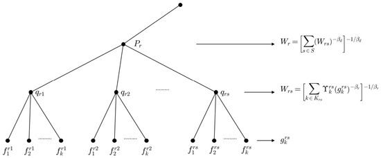
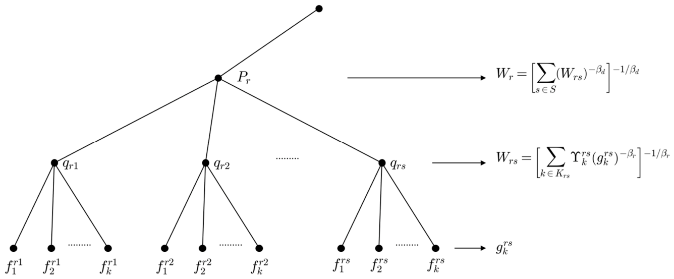
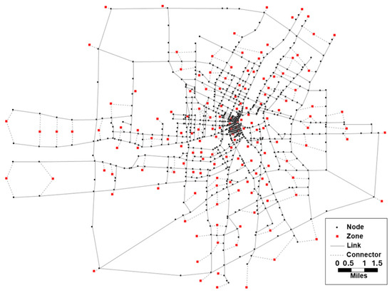
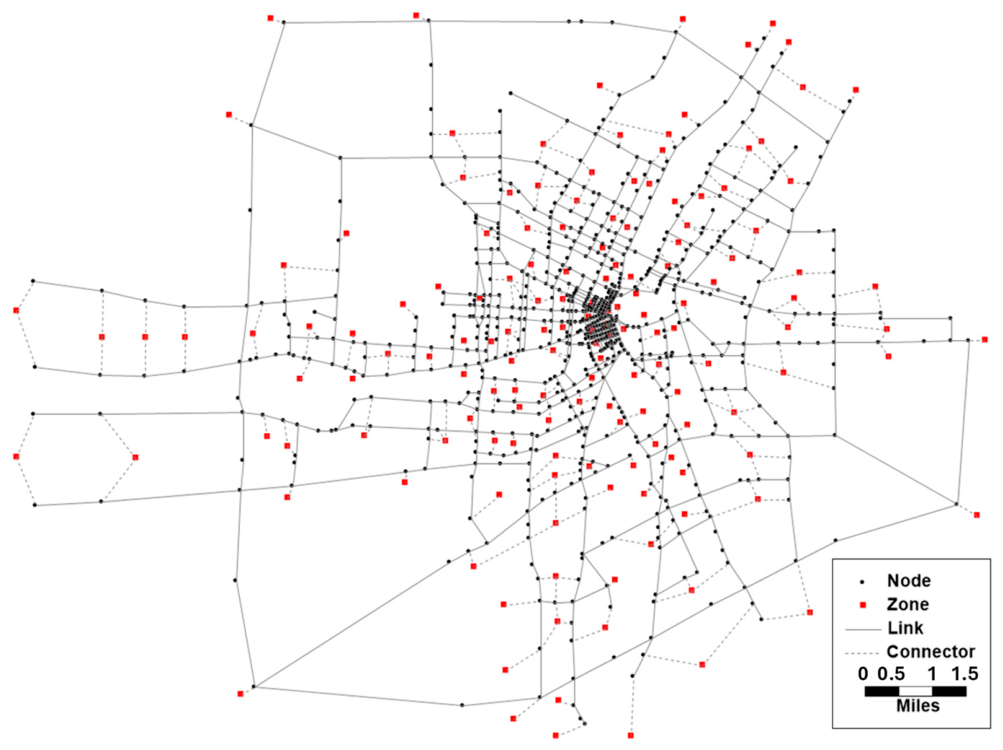
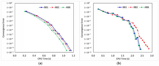
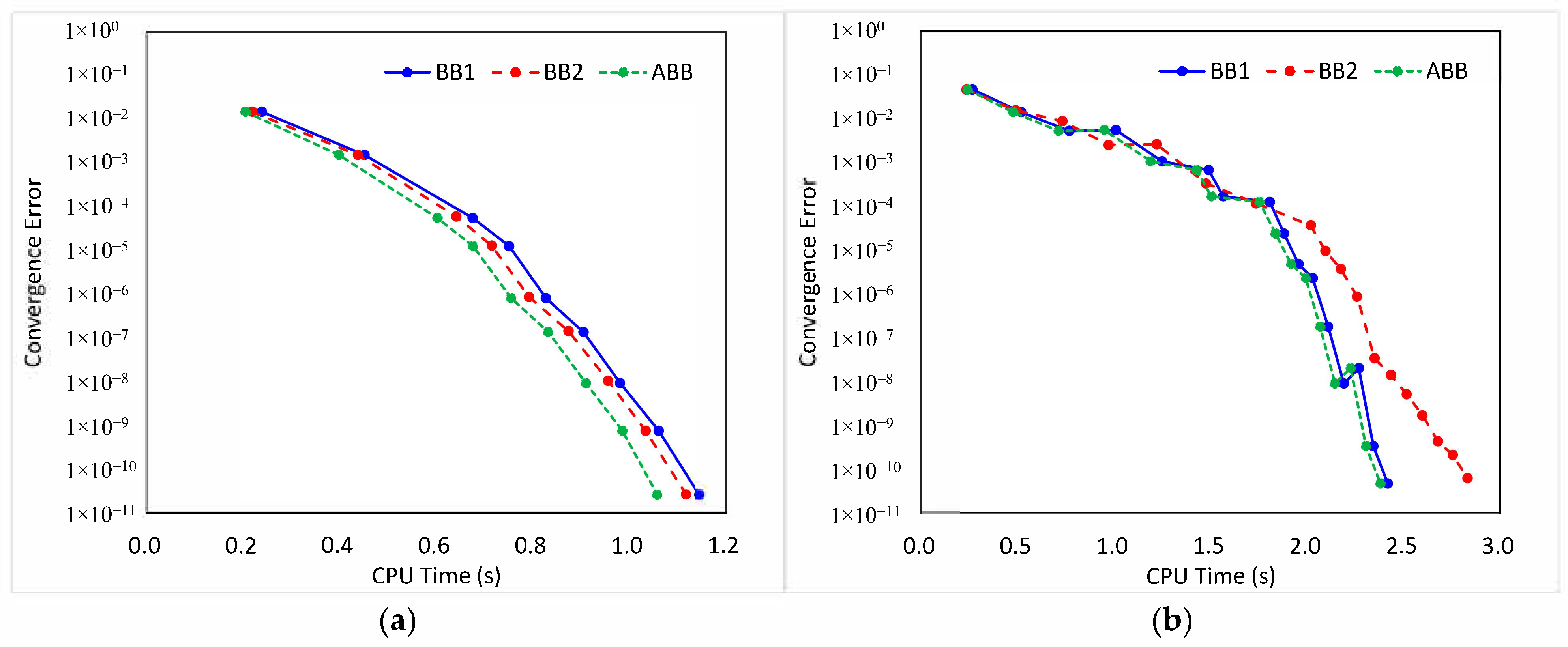
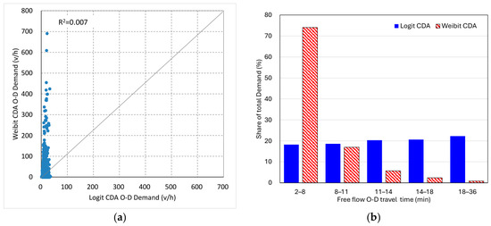
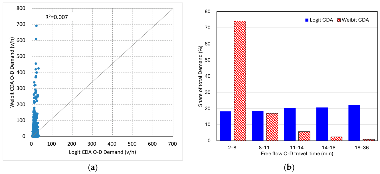
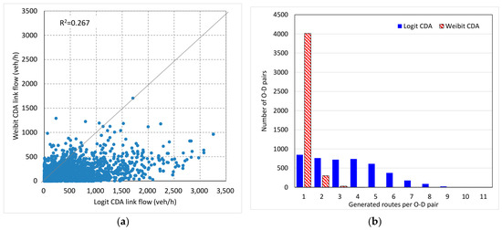
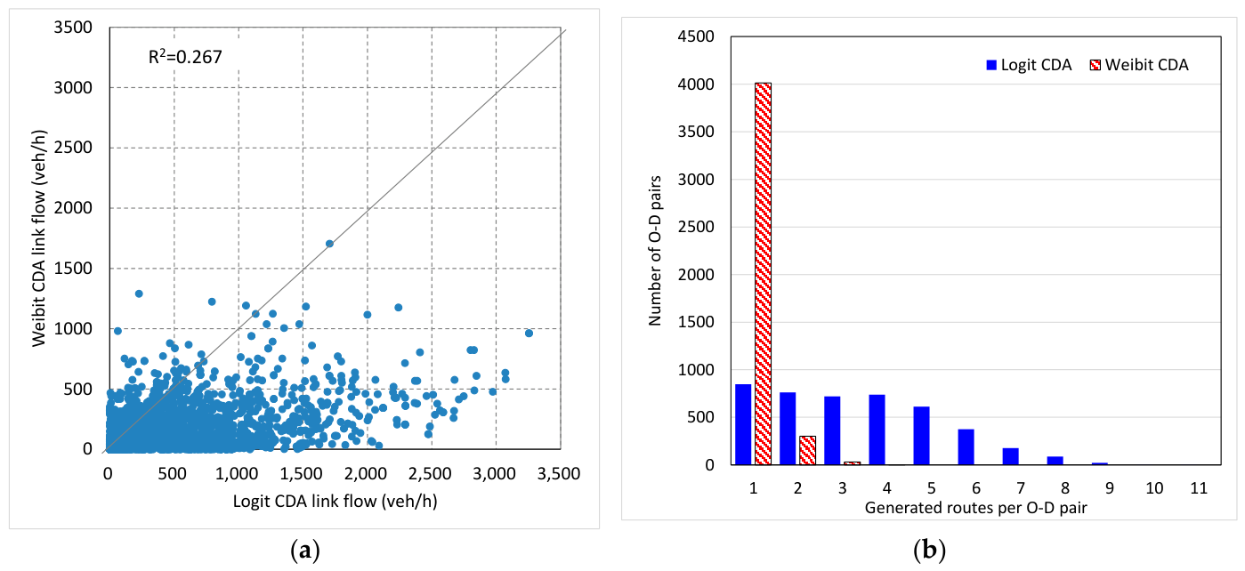
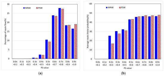
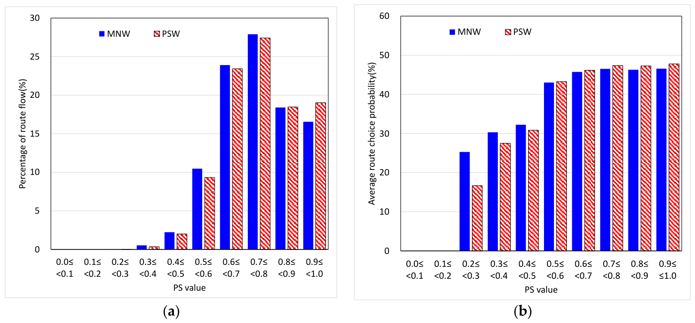

Disclaimer/Publisher’s Note: The statements, opinions and data contained in all publications are solely those of the individual author(s) and contributor(s) and not of MDPI and/or the editor(s). MDPI and/or the editor(s) disclaim responsibility for any injury to people or property resulting from any ideas, methods, instructions or products referred to in the content. |
© 2026 by the authors. Licensee MDPI, Basel, Switzerland. This article is an open access article distributed under the terms and conditions of the Creative Commons Attribution (CC BY) license.