


Abstract
Binocular camera calibration is the core foundation of 3D vision technology, and its performance directly determines the accuracy of subsequent tasks. Zhang’s checkerboard method relies on calibration targets and suffers from poor scene adaptability, whereas conventional Kruppa self-calibration is prone to parameter divergence, low accuracy, and slow convergence. To address these issues, this paper proposes a boardless stepwise self-calibration method for binocular cameras based on an improved Kruppa equation. The method introduces (1) a stepwise decoupled optimization strategy that alternates between intrinsic and distortion parameters, combined with a SIFT + bidirectional FLANN + RANSAC + Census feature pipeline; (2) a multi-constraint regularization framework that enforces focal-length consistency, principal-point bounds, and a distortion penalty; and (3) an entropy-based feature-coverage criterion with inheritance-based batch tuning for streaming production-line images. Experiments on 800 binocular pairs from a laboratory-simulated pin-shaft production line show that the proposed method achieves an average reprojection error of 0.52 px, an 83.6% reduction over the traditional Kruppa method, approaching Zhang’s calibration. The stepwise solver converges within 7.4 inner iterations per batch, versus 23.31 iterations for the Kruppa baseline. In an end-to-end pin-shaft length measurement task, the mean absolute error is 3.01 mm, on par with Zhang’s calibration and well within the ±5 mm industrial tolerance; even under strong vibration-blur interference, the error remains 3.32 mm.
1. Introduction
The main function of camera calibration is to achieve the mapping relationship from 2D images to 3D scenes, and recover the 3D information of the scene from the 2D images captured by the camera. The specific content of camera calibration includes solving the camera’s intrinsic parameter matrix, pose parameters, distortion parameters and other related information.
Camera calibration methods are mainly divided into two categories: traditional calibration methods and self-calibration methods. Traditional calibration methods require manually fabricated calibration objects with strictly restricted shape and size. Then, the camera parameters are solved by establishing the constraint relationships between the point coordinates of the calibration object and their corresponding image points. This type of method has the advantages of high calibration accuracy and strong reliability. However, due to the need for a calibration object, its application environment is limited, making it unsuitable for camera calibration without a calibration board. Faugeras first proposed the concept of camera self-calibration in the early 1990s, which made it possible for camera calibration to be independent of the scene position and camera motion [1]. The theory of camera self-calibration is based on the inherent constraint relationships of the camera’s intrinsic parameters. These constraint relationships are only related to the camera’s intrinsic parameters and are independent of the camera’s motion posture and the structure of the scene where it is located.
In the automated production lines of pin shaft parts, binocular vision systems are widely deployed in critical applications such as inspection, assembly guidance, and quality evaluation, owing to their low cost and capability to accurately acquire 3D information [2]. However, the complex production-line environment—including vibration, oil contamination, and dynamic workpiece interference—renders calibration-board-based traditional methods difficult to apply. Moreover, the placement of calibration boards may disrupt the production flow, and frequent mechanical vibrations can cause drift in the camera’s intrinsic and extrinsic parameters, necessitating periodic recalibration [3]. More importantly, binocular images captured in real scenarios often suffer from severe lens distortion, uneven illumination, and sparse feature points, further compounding the calibration difficulty [4]. Traditional camera calibration methods recover parameters by establishing the geometric mapping between 3D world coordinates and 2D image coordinates; a representative example is Zhang’s planar calibration method [5,6], which uses checkerboard images captured at multiple poses and solves for intrinsic and extrinsic parameters via homography matrix decomposition. However, it relies on high-precision calibration boards and static imaging conditions, making it ill-suited for dynamic pin-shaft production lines.
To eliminate the dependence on calibration targets, Hartley proposed a Kruppa-equation-based self-calibration method [7] that recovers intrinsic parameters from the singular-value constraints of the fundamental matrix without requiring known 3D structures. Nevertheless, the traditional Kruppa approach is extremely sensitive to image noise and feature matching errors, and the severe coupling among intrinsic, distortion, and extrinsic parameters frequently leads to optimization divergence or low accuracy in strongly distorted industrial images. Recent advances have partially addressed these limitations through rectification homography optimization [8] and hybrid cost-function fusion [9], while event-based calibration methods [10] have demonstrated fast parameter estimation under high-speed motion; however, these approaches remain less mature for conventional industrial frame cameras.
With the development of deep learning, researchers have started regressing camera parameters directly with neural networks. Bogdan et al. pioneered an end-to-end camera calibration network that predicts intrinsic parameters from a single image via a convolutional architecture [11]. However, it relies on extensive annotated data and exhibits limited generalization ability. Subsequent efforts have attempted to alleviate this data dependency through synthetic training data and domain adaptation [12], recent learning-based frameworks such as StereoGeo [13] pursue pattern-free stereo calibration via joint intrinsic–extrinsic estimation. Nevertheless, these data-driven methods still rely on large annotated training datasets and suffer from severe domain shift when migrated to low-texture industrial scenes with strong lens distortion.
Self-supervised learning constructs supervision signals through the geometric or statistical characteristics of data itself, avoiding manual annotation [14]. DSO proposed by Engel achieves uncalibrated visual odometry using photometric consistency constraints, providing ideas for self-supervised calibration [15]. In binocular systems, epipolar geometry constraints are widely used to replace supervision signals [16]. For example, Ummenhofer trained a stereo matching network using epipolar line constraints without depth annotation; this paper further applies this constraint to camera parameter estimation, constructing a self-supervised loss through reprojection error to adapt to the characteristics of real industrial images [17]. However, most self-supervised methods focus on visual odometry or depth estimation rather than precise camera calibration, and their parameter estimation accuracy is insufficient for industrial dimensional measurement tasks.
The particularities of industrial images place higher demands on calibration methods: complex distortion induced by close-range shooting of pin shafts leads to obvious radial and tangential lens distortion, which cannot be fully modeled by conventional polynomial distortion models [18]; complex surface characteristics, including workpiece reflection and oil contamination, bring severe matching noise and outliers, raising requirements for robust feature constraint strategies [19].
Targeting the above research gaps and the particularity of on-site industrial scenes, we propose a stepwise self-calibration method for binocular cameras based on improved Kruppa equations. Relying solely on natural production-line images without calibration boards, the method introduces multi-constraint regularization and stepwise decoupled optimization to suppress noise and mitigate distortion effects. The main contributions are summarized as follows:
(1) We employ a gradual decoupling approachWe employ a gradual decoupling approach within the Kruppa framework. In the joint formulation, the residual couples the intrinsic and distortion parameters through the undistortion mapping, and the sensitivities of both parameter groups scale with the radial distance from the principal point. Their effects on the epipolar residuals are therefore similar in direction, so the two groups compete in the optimization and the Gauss–Newton updates become sensitive to noise in the feature matches rather than being dominated by geometric structure. This is evidenced in Section 3, where the baseline Kruppa result drifts by approximately 15% in despite converging to a small residual. By solving for first with distortion fixed at zero, and then for with intrinsics frozen, this interference between the two groups is avoided.
(2) We embed hardware-physical constraints directly into the Kruppa residual, rather than treating them as post-hoc regularization. The standard Kruppa equation alone provides only two scalar constraints per stereo pair, leaving the solution space under-determined. We add three constraint terms—inter-camera focal-length consistency, principal-point proximity to image center, and an L2 distortion penalty—to the residual vector, which bounds the solution to the hardware-feasible region and eliminates the unconstrained drift observed in the baseline.
(3) We introduce a Census texture-consistency check into the Kruppa matching-pipe stage as a photometric gate: it rejects correspondences that survive geometric RANSAC but exhibit inconsistent local intensity patterns between the left and right views. Unlike Census in conventional stereo matching, here it is used as a Kruppa-inlier gating criterion rather than a disparity cost.
(4) We pair entropy-based feature-coverage evaluation with an inheritance-based batch refinement, enabling continuous recalibration from streaming production-line imagery without manual board deployment.
2. Materials and Methods
2.1. Experimental Setup
To verify the effectiveness of the proposed stepwise self-calibration method for binocular cameras without a calibration board, we evaluate its performance in terms of calibration accuracy and convergence efficiency using a laboratory setup that simulates a real pin-shaft production line. We use the first-generation ZED binocular industrial camera (Stereolabs Inc., San Francisco, CA, USA), with a monocular resolution of 2208 × 1242 at 15 fps, a focal length of approximately 2.8 mm, and a baseline of 120 mm. The computing platform comprises an Intel Core i5-8700K CPU (Intel Corporation, Santa Clara, CA, USA), an NVIDIA P100 GPU (NVIDIA Corporation, Santa Clara, CA, USA), 16 GB RAM, and Windows 10 (Microsoft Corporation, Redmond, WA, USA); the software environment is Python 3.8 with OpenCV 4.9.0. The binocular camera is rigidly mounted on an aluminum alloy bracket in a top-down configuration directly above the workpiece, matching the camera mounting geometry of real pin-shaft production lines where cameras are installed above processing stations for workpiece type recognition and robotic arm grasping guidance. The working distance from the camera optical center to the measured pin-shaft surface is 435 mm, at which the field of view is approximately 690 mm × 390 mm.
Image acquisition is performed under natural indoor lighting simulating a factory workshop, without supplementary illumination. Auto-exposure and auto white balance are disabled to ensure consistent imaging across all captured frames, and the left and right cameras are synchronized via the ZED’s built-in hardware trigger.
Our laboratory setup replicates the core operational characteristics of a real pin-shaft production line: as in actual machining, natural ambient lighting is used without supplemental illumination, the camera is mounted in a top-down configuration, and the workpieces have metallic finish-machined surfaces. The main difference is that in a real production line the binocular camera is integrated into the machining equipment above the workstation, whereas our laboratory setup mounts the camera on an independent stand with a reduced working distance for experimental convenience. The dataset focuses on static scenarios simulating practical pin-shaft applications, as shown in Figure 1b, with the corresponding real production-line scenario presented in Figure 1a. The scene objects mainly include low-texture smooth cylindrical surfaces, unmarked solid-color-coated surfaces, and finish-machined end faces.
Figure 1.
Laboratory-simulated real data collection scenario of the pin shaft production line: (a) real scenario of the pin shaft production line; (b) laboratory simulation scenario.
2.2. Experimental Dataset
To ensure the comprehensiveness of verification, two types of datasets are adopted in the experiment. The real-scene dataset initially consists of 800 pairs of binocular images captured by synchronous triggering of the left and right cameras, with natural light as the illumination condition and a solid-color background configured. The image resolution is uniformly scaled to 2208 × 1242. All images are captured as non-consecutive stereo pairs. To ensure uniform spatial distribution of feature points across the entire image plane, the same pin shaft workpiece is manually repositioned to different locations within the field of view between each capture, while the binocular camera remains rigidly fixed throughout the data collection process.
A multi-step filtering procedure is applied to remove low-quality image pairs: (1) images with noticeable motion blur or out-of-focus blur are discarded by visual inspection; (2) image pairs with fewer than 14 valid SIFT feature matches are filtered out. After filtering, approximately 700 high-quality stereo pairs remain and are used in this study. To avoid biased performance evaluation, these valid image pairs are randomly split into two subsets: a calibration subset of 560 pairs used exclusively for optimizing camera intrinsic and distortion parameters, and an independent test subset of 140 pairs reserved solely for evaluating calibration accuracy via reprojection error. No images from the test subset are involved in the parameter optimization process. Without relying on a calibration board, calibration is achieved solely through feature point matching in natural scenes, and part of the dataset is shown in Figure 2.
Figure 2.
Partial experimental datasets: (a) left-view image of the pin shaft scene; (b) right-view image of the same scene; (c) zoomed view of a pin shaft surface; (d) zoomed view of pin shaft surfaces.
The standard calibration board dataset is used for comparing calibration accuracy, for which 20 sets of checkerboard calibration board images with checkerboard specification 7 × 5 and square size 40 mm are synchronously collected. These images are applied to solve parameters via Zhang’s calibration method, serving as a reference for true values, and part of the dataset is shown in Figure 3.
Figure 3.
Partial calibration board-based datasets: (a) left-view image of the checkerboard calibration target; (b) right-view image of the same target.
2.3. Theoretical Foundation
In the binocular camera calibration system, the camera model serves as the core theoretical foundation running through parameter solution and accuracy optimization. To clarify the theoretical basis of the proposed stepwise self-calibration algorithm, this section elaborates on the basic principles of the camera imaging model, Kruppa equation and epipolar geometric constraint.
2.3.1. Camera Model
The intrinsic parameter matrix describes the conversion between the camera coordinate system and the pixel coordinate system and is the target of Kruppa-based calibration. The standard 3 × 3 intrinsic matrix is adopted as (1):
where , are the focal lengths of the camera in the x-axis and y-axis directions, respectively, and , are the principal point coordinates of the camera. The projection model between the world coordinate system and pixel coordinate system is defined as (2):
where R is a 3 × 3 rotation matrix, t is a 3 × 1 translation matrix.
In this paper, the Brown–Conrady distortion model is adopted [20], which is the most widely used standard distortion model in industrial binocular vision. This model includes radial distortion coefficients , and tangential distortion coefficients , , and is consistent with calibration framework of OpenCV industrial cameras [21]. Recent comparative studies of geometric camera calibration [22] confirm that the Brown–Conrady model remains the most practical choice for industrial close-range imaging.
2.3.2. Kruppa Camera Calibration Method
The core of the Kruppa method lies in constructing constraint equations by leveraging the singular value properties of the essential matrix E. In the case where camera distortion is not considered, the constraint equation of the essential matrix can be derived based on the fact that the projection of epipolar lines onto the image of the absolute conic should remain consistent, as shown in (3).
The essential matrix encodes the relative pose between two cameras and can be decomposed as (4).
where R is the 3 × 3 rotation matrix, is the translation vector, and stands for the skew-symmetric matrix constructed from t. Define the image of absolute conic as . Based on this geometric invariant, the standard Kruppa constraint equation is established as (5).
Only two linearly independent scalar constraints can be extracted from a single stereo image pair, which imposes two constraints for solving . Since the symmetric matrix contains five independent unknown entries, at least three groups of matched stereo image pairs are required to generate six independent equations for complete solution of .
2.3.3. Epipolar Constraint
Traditional Kruppa equation methods are mostly used to solve the camera’s intrinsic parameter matrix and do not account for camera distortion. To solve camera distortion while estimating intrinsic parameters, the epipolar constraint is introduced.
For binocular matching points, the original points need to undergo undistortion processing to obtain ideal points, as shown in (6) and (7).
Among them, denotes the ideal point of the camera, denotes the original point of the camera, denotes the distortion parameters of the camera, and then the epipolar constraint can be expressed as (8):
Therefore, each matching point can provide one constraint condition. According to the camera model, the total number of unknowns for the camera’s intrinsic parameters and distortion parameters is 16, and the Kruppa equations can provide 2 constraint conditions. Thus, the number of matching points must be at least 14.
2.4. Proposed Algorithm
Unlike existing algorithms, the proposed method adopts a stepwise decoupled optimization strategy. Firstly, physically reasonable initial intrinsic parameters are obtained through multi-constraint optimization; the intrinsic parameters are then fixed to optimize the distortion coefficients. Furthermore, an inheritance-based batch refinement mechanism supports the continuous input of small-batch data for iterative parameter correction. Compared with the traditional Kruppa method, Census verification is added to feature point matching to improve the accuracy of corresponding points, and physically motivated constraints are incorporated into the residual function design. Together, these designs address the poor convergence, low robustness, and limited applicability of the traditional Kruppa method.
The necessity of stepwise decoupling in the Kruppa framework can be understood from the Jacobian structure. In the joint formulation, the residual couples intrinsic and distortion parameters through the undistortion mapping. The sensitivities both scale with the radial distance from the principal point, so the corresponding Jacobian columns are nearly collinear. Numerically, this causes Gauss–Newton direction updates to be dominated by noise in the feature matches rather than by geometric structure, as demonstrated in Section 3; the baseline Kruppa result drifts by approximately 15% in despite converging to a small residual. By solving for first with distortion fixed at zero, and then for , with intrinsics frozen, this collinearity is removed.
2.4.1. Obtain Intrinsic Parameters via Multi-Constraint Optimization
There is a strong coupling relationship between the focal length, principal point, and distortion coefficients in the camera’s intrinsic parameters. That is, distortion correction depends on intrinsic parameters, while intrinsic parameter estimation is affected by distortion. If both are optimized simultaneously, the optimization is prone to falling into a local optimum due to mutual interference between variables. Therefore, before optimizing the camera’s intrinsic parameters, distortion is temporarily ignored, focusing on optimizing the focal length and principal point. Physical prior constraints are used to limit the intrinsic parameters within a reasonable range—for example, the principal point is close to the image center, and the focal lengths of the left and right cameras are approximately equal—providing reliable benchmark intrinsic parameters for subsequent distortion optimization.
Extract Image Matching Point Pairs
Compared with traditional algorithms, this paper adds Census verification to feature extraction and matching to improve the matching accuracy of corresponding points. The extraction method for initial matching points still adopts the SIFT+FLANN+RANSAC approach. After optimization via the RANSAC method, Census verification is further added to screen the matching points.
The Census transform has been widely adopted in stereo matching for its robustness to monotonic illumination changes [23], and improved Census-based cost aggregation methods have been shown to improve matching reliability under challenging illumination conditions [24]. The Census transformation compares the target pixel in a grayscale image with other pixels in the transformed region. The comparison results are represented by 0 and 1, thereby generating a Census transformation sequence composed of 0 and 1. The specific generation formula can be expressed as (9).
where denotes the Census transformation sequence generated by the pixel P, ⊗ denotes the concatenation operation, represents the Census region corresponding to the pixel P, and is calculated as (10).
where denotes the intensity of pixel P. Generally speaking, P is not included in , because . The sequence formed after the Census transformation is the Census sequence. The difference between different pixels can be determined by calculating the Hamming distance between the Census sequences formed by different pixels. A smaller Hamming distance indicates a smaller difference between the two pixels, while a larger distance indicates a greater difference. Hamming distance is calculated by (11).
After Census verification, outliers among the feature matching points can be effectively eliminated, as shown in Figure 4.
Figure 4.
Comparison of matching points between the traditional and improved pipelines: (a) matching points of traditional pipelines; (b) matching points of improved pipelines(the rectangle highlights a representative mismatched pair that disappears after Census verification).
Improved Residual Function in the Intrinsic Parameter Solving Stage
Simultaneously optimizing a nonlinear equation with 8 parameters is highly prone to falling into a local optimal solution. To address this, this paper optimizes the traditional residual function by adding practice-based physical constraints, including the principal point constraint residual and the focal length ratio constraint residual. Meanwhile, the traditional Kruppa equation residual and epipolar residual are also incorporated into the residual function.
The Kruppa residual function adopted in paper is the same as the traditional one, as shown in (12). Here, denotes flattening the matrix into a vector, and F represents the Frobenius norm of the matrix.
The two cameras of a binocular camera system are generally from the same production line batch. Therefore, the focal lengths of the two cameras do not differ significantly. Additionally, the focal lengths on the x-axis and y-axis should be as close as possible. To this end, we designed the focal length ratio constraint residual, as shown in (13). The specific meaning is that the closer the ratio of the relevant parameters of the two cameras is to 1, the smaller the residual, and the better it satisfies the hardware consistency of focal lengths.
Similar to the focal length constraint, the principal point of a general camera is near the center of the camera image. Therefore, in addition to the physical constraint on focal length, this paper also adds the principal point constraint, as shown in (14), where denote the width and height of the image, respectively.
Both the principal point constraint and the focal length constraint belong to the physical constraints for calibration. In addition to the camera’s physical constraints, compared with the traditional residual function, this paper also incorporates the epipolar residual into consideration, as shown in (15). Among them, the first squared term inside the square root represents the algebraic error of the epipolar constraint, and the latter two terms are the geometric errors of the epipolar constraint, specifically referring to the distance from the matching point to the epipolar line.
The finally adopted residual function includes four parts, as shown in (16), and the corresponding residual vector is presented in (17). All residual terms are normalized results.
Solving for Optimal Intrinsic Parameters via the Least Squares Method
In the previous section, a multi-constraint residual model was constructed. The residual function has a nonlinear relationship with the parameters to be optimized. It cannot directly obtain a closed-form solution like linear least squares, and the optimal solution must be found through iterative approximation. Therefore, this paper adopts the nonlinear least squares optimization framework to minimize the residual-based objective function and selects the Levenberg–Marquardt algorithm with trust-region reflection for intrinsic parameter solving. Combining the merits of gradient descent and the Gauss–Newton method, this algorithm features built-in adaptive damping control to adjust iterative step sizes automatically, which balances convergence stability and convergence speed.
When optimizing multi-source nonlinear residuals with distinct nonlinear strengths, the solver dynamically adjusts its internal iterative strategy. The resulting convergence behavior is quantified in Section 3. The whole optimization process relies on two native built-in modules of the TRF-LM solver: Jacobian matrix approximation and iterative update direction calculation.
The residual terms constructed in this paper contain strongly nonlinear operations. Deriving analytical derivatives for such mixed nonlinear residuals is complex and prone to numerical singularity. The three-point central finite-difference scheme with adaptive step size mitigates this, and the trust-region radius prevents large steps that would amplify finite-difference noise, as shown in Equation (18).
In Equation (18), denotes the intrinsic parameter to be optimized, is the internal fixed scale factor, and represents the minimum reference offset, which avoids the step size approaching zero for small parameter values. On the basis of the adaptive step size, three-point numerical central differentiation is adopted to compute partial derivatives, as shown in Equation (19):
In Equation (19), e is the unit vector, and J represents the assembled Jacobian matrix. Due to the obvious nonlinear differences among multi-source residuals, the TRF-LM algorithm introduces a damping factor to balance the Gauss–Newton direction and gradient descent direction, and the unified update formula is shown in Equation (20):
Among them, denotes the Gauss–Newton approximate Hessian matrix; the damping factor is automatically adjusted by the solver to adapt to the overall nonlinearity of residuals.
2.4.2. Obtaining Distortion Parameters via Multi-Constraint Optimization
All distortion solving and correction processes in this work are implemented based on the unified Brown–Conrady standard model and analytical inverse mapping strategy, ensuring the unity and traceability of distortion modeling. Distortion causes image points to deviate from their ideal projection positions, undermining the geometric constraints and matching accuracy of the stereo camera. Therefore, on the basis of intrinsic parameter optimization, distortion parameters need to be solved through multi-constraint collaborative optimization. Compared with intrinsic parameter optimization, distortion parameters have a stronger nonlinear relationship with the residual function, and the parameters must satisfy strict physical range constraints. Thus, a targeted residual function and optimization strategy need to be constructed.
Residual Function in the Distortion Solving Stage
Using the method described in Section 2.4.1, this paper has obtained the basic estimation of camera intrinsic parameters. Therefore, it is necessary to modify the residual function when correcting the distortion parameters—removing the original terms based on physical constraints and adding a regularization constraint. The L2 norm is used to suppress excessively large absolute values of distortion parameters, thereby avoiding overfitting. The calculation method of the regularization constraint residual is as shown in (21).
Among them, is the regularization coefficient. Through the form of regularization constraining distortion, the optimization process naturally tends to select smaller distortion parameters—which conforms to the actual distortion characteristics of the lens and achieves the goal of suppressing unrealistic distortion. An excessively large will over-suppress real lens distortion and cause under-fitting, while an excessively small cannot effectively restrain unreasonable distortion values and leads to over-fitting. In this work, the optimal value of is set as 0.1. Therefore, the design of the residual function in the stage of multi-constraint distortion function solving is as shown in (22).
Solving for Distortion Parameters via the Least Squares Method
Consistent with the least squares matrix used in updating the intrinsic parameter matrix, the same LM formula is still adopted in the distortion parameter solving stage, as shown in (19) and (20). However, due to the stronger nonlinearity in the process of solving distortion parameters, the differences only lie in the design of the variables to be optimized, residual composition, and initial values of the least squares method. These configuration differences are determined by the different physical characteristics of intrinsic parameters and distortion coefficients, ultimately serving the core goals of step-by-step calibration, avoiding parameter coupling, and improving convergence accuracy. Compared with the least squares stage for intrinsic parameters, the main differences of the least squares method for solving distortion parameters are shown in Table 1.
Table 1.
Comparison between the distortion solving stage and the intrinsic solving stage.
2.4.3. Parameters Are Continuously Optimized via the Inheritance Method
Inherited parameter optimization is based on the optimal intrinsic parameters and distortion parameters calibrated in the previous stage, and continuously approaches the true camera parameters through the logic of iterative inheritance and gradual correction. To ensure the effectiveness of the optimization process, it is necessary to establish a targeted evaluation index system to quantify the parameter optimization effect.
Solving for Parameters via the Least Squares Method
Due to the relatively strict implementation standards adopted in the feature point collection process of this paper, the number of feature points in a single set of images is relatively small. It is therefore necessary to combine multiple sets of images to complete parameter solving. To evaluate the coverage of the feature point combination from multiple sets of images on the entire image, the entropy method is adopted for feature point evaluation.
Figure 5 shows the overview of the proposed stepwise self-calibration pipeline. Among them, the entropy formula for judging the distribution of feature points is shown in (23).
where N denotes the number of grids, represents the proportion of the number of feature points in the i-th grid to the total number of feature points, and H is the normalized entropy value. This formula can reflect the distribution of feature points in the image: the more uniform the feature point distribution, the larger the entropy value; the more concentrated the feature point distribution, the smaller the entropy value. The value of N should be moderate: overly coarse grids fail to capture local small-scale concentration, while overly fine grids will result in a zero proportion of feature points in most grids in scenarios with few feature points, leading to distortion in entropy calculation. The images used in this work have an original resolution of 2208 × 1242. Dividing the image into an 8 × 6 grid makes each grid cell approximately 276 × 207 pixels, which matches the distribution range of SIFT feature points in pin shaft production line images. A coarser grid cannot reflect local feature aggregation, while a finer grid will generate excessive empty cells. Figure 6 shows the entropy change after applying the multi-image coverage method, where (a) illustrates the feature point distribution and entropy value of a single set of images, (b) presents the feature point distribution and entropy value of multiple sets of images after meeting the feature point distribution requirements, and (c) shows how the normalized entropy of the accumulated matching set grows as more image pairs are added, crossing the acceptance threshold after 6 image pairs, which determines the batch size in the entropy-based selection step.
Figure 5.
Overview of the proposed stepwise self-calibration pipeline.
Figure 6.
Comparison of entropy changes after applying multi-image coverage: (a) feature points and entropy value of a single set of binocular images; (b) feature points and entropy value of multiple sets of binocular images meeting the requirements; (c) entropy growth with multi-image coverage.
Continuous Tuning of Parameters via the Inheritance Method
Because continuous binocular image acquisition via video is feasible in practical production, a large number of images usable for training can be obtained to continuously tune camera parameters. Thus, for the uncalibrated stereo calibration scenario, this paper proposes an inheritance method for parameter tuning. Its core logic is to inherit the calibration parameters of the previous batch as initial values, combine the feedback of feature point distribution entropy, and gradually converge to the optimal parameters through batch-wise iterative optimization. The tuning process of the inheritance method is divided into three steps: parameter initialization, batch-wise iterative optimization, and convergence verification & optimal parameter determination.
In the parameter initialization phase: If it is the first tuning, image size-adaptive initialization is adopted—the focal length is set to 0.5 times the image diagonal, the principal point is set near the image center, and the distortion coefficients are initialized to 0. If there are previous batch calibration results, the intrinsic parameter matrix and distortion coefficients of the previous batch are directly inherited as the initial values of the current batch, avoiding low convergence efficiency caused by repeated optimization.
In the batch-wise iterative optimization phase: Image pairs are divided into batches according to the method described in "Solving for Parameters via the Least Squares Method", and then a distributed optimization strategy is implemented. Specifically, first fix the distortion coefficients to optimize the intrinsic parameters; then fix the intrinsic parameters to optimize the distortion coefficients. After each batch of optimization, the calibration parameters of the current batch are saved as the initial inherited values for the next batch, forming an iterative chain.
In the convergence verification & optimal parameter determination phase: the iteration terminates when the variation of intrinsic parameters is less than 5 pixels and the variation of distortion coefficients is less than 0.1 for three consecutive batches. Meanwhile, the intrinsic parameters, distortion coefficients, and extrinsic parameters of this batch are saved.
Convergence analysis. The proposed iterative scheme converges at three nested levels.
Inner level. The trust-region reflective algorithm is applied to a bounded least-squares problem with a smooth residual (Brown–Conrady undistortion is analytic except at the optical center, which is excluded by the principal-point constraint). For such problems, the TRF method is guaranteed to produce a non-increasing residual sequence and to converge to a stationary point from any reasonable initialization [25]. The adaptive damping factor prevents the Gauss–Newton step from overshooting when the Jacobian becomes ill-conditioned.
Stage level. Because Stage B resolves only the distortion subproblem with the Stage A intrinsics frozen, its search space is a restricted manifold; the epipolar residual evaluated on the held-out image pairs monotonically decreases within Stage B, and the frozen intrinsics are not perturbed. This restricted-subproblem structure avoids the coupled oscillation observed when intrinsics and distortion are optimized jointly from initialization.
Outer level. Each outer batch initializes from the converged parameters of the previous batch. The batch-wise residual is a running average over newly sampled image pairs, and the algorithm terminates when the parameter drift falls below the 5-pixel/0.1 thresholds for three consecutive batches. Empirically, this takes 17 batches; the monotone non-increasing behavior is visible, where the residual does not exhibit the late-stage oscillation typical of unconstrained Kruppa.
3. Results
3.1. Experimental Results and Analysis
In the experiment, the hyperparameter configuration adopted by the algorithm proposed in this paper is as shown in Table 2.
Table 2.
Parameters adopted in the experiment.
The selection rationale for the key hyperparameters in Table 2 is as follows.
The Census transform window size of 5 × 5 and the RANSAC confidence probability of 0.9 are adopted as standard default values widely used in stereo vision feature matching pipelines [26]. The normalized entropy threshold is set to 0.7, based on the observed entropy distribution of image pairs in our dataset, which typically ranges from 0.5 to 0.8. A threshold higher than 0.7 causes the number of image pairs per batch to saturate at the maximum limit of 30, leading to redundant computation, while a threshold lower than 0.7 results in too few image pairs per batch and degraded fitting performance. The value of 0.7 provides a balanced trade-off between feature coverage sufficiency and computational efficiency. The RANSAC epipolar inlier threshold of 0.2 pixels is selected to balance matching precision and computational efficiency. A threshold larger than 0.2 admits a large number of outlier correspondences, increasing the computational burden of subsequent Census filtering and introducing residual mismatches even after verification. A threshold smaller than 0.2 excessively rejects valid feature points, resulting in an insufficient number of constraints for robust parameter estimation.
To verify the stability of the proposed method with respect to the regularization coefficient , we conduct sensitivity analysis by varying from 0.01 to 1.0 while fixing all other hyperparameters, with the results summarized in Table 3.
Table 3.
Sensitivity analysis of .
As shown in Table 3, when is smaller than 0.1, the reprojection error remains low, but the number of inner iterations increases significantly, indicating that under-regularization leads to slower and more oscillatory optimization. When exceeds 0.1, the reprojection error gradually increases because excessive regularization suppresses the geometric constraint terms and prevents the optimization from converging to the true geometric solution. The chosen value of achieves the best trade-off between convergence speed and final accuracy. Overall, the calibration accuracy remains within a reasonable range when deviates moderately from the chosen value, demonstrating that the proposed method is not highly sensitive to this hyperparameter.
In the experiment, Zhang’s calibration method, the traditional Kruppa self-calibration method, and the recently proposed supervised calibration approach DroidCalib [27] are selected as comparison baselines to comprehensively evaluate the performance of the proposed algorithm on real captured industrial datasets. The core evaluation metrics cover intrinsic parameter estimation precision, distortion correction performance, and average reprojection error. The relative deviation between each algorithm’s solved parameters and the reference values from Zhang’s checkerboard calibration is adopted to quantify the estimation accuracy of intrinsic and distortion coefficients, while the average reprojection error characterizes the overall reliability of the calibrated camera parameters. To evaluate the stability of each calibration method, all experiments are repeated 5 times with randomly selected image subsets, and the mean values across the 5 runs are reported in Table 4, with standard deviations shown in parentheses. Table 4 summarizes the key quantitative results of all four calibration schemes.
Table 4.
Comparison of intrinsic parameters obtained by different algorithms.
Intrinsic parameters constitute the core of camera calibration and dominate the precision of subsequent three-dimensional reconstruction and dimensional measurement. In Table 4, the intrinsic parameter accuracy of the proposed algorithm outperforms traditional Kruppa self-calibration and DroidCalib, and approaches the benchmark results from Zhang’s checkerboard calibration. For focal lengths of and , the relative deviations of our method are controlled within 0.9%, while traditional Kruppa yields deviations exceeding 14%. As a data-driven self-supervised scheme, DroidCalib suffers severe domain shift when migrated to low-texture industrial scenes, leading to larger focal length estimation errors. Benefiting from entropy feature screening, Census outlier elimination and multi-constraint optimization, our method alleviates parameter coupling in Kruppa equations and avoids the generalization degradation of learning-based calibration in industrial environments.
Lens distortion deforms peripheral image content and degrades feature matching and epipolar constraint reliability. Different from the relative deviation used for the intrinsic parameters, we adopt absolute error to evaluate distortion coefficients for higher comparability, given the inherently small magnitude of distortion terms. The proposed algorithm achieves smaller absolute errors on all distortion coefficients compared with traditional Kruppa and DroidCalib. By introducing decoupling optimization between intrinsic and distortion parameters, our method suppresses abnormal overestimation of distortion values.
Average reprojection error is the comprehensive metric reflecting overall calibration quality, where a smaller value indicates more reliable solved camera parameters. According to statistical results, the average reprojection error of the proposed algorithm is 0.52 pixels, clearly superior to 3.18 pixels of traditional Kruppa and 0.89 pixels of DroidCalib, and slightly higher than Zhang’s reference value of 0.25 pixels. This advantage originates from the robust matching purification pipeline and multi-constraint residual optimization strategy adopted in this work. After screening unreliable correspondences via entropy pre-filtering and Census matching verification, the optimized parameters fit epipolar geometry more accurately.
To quantitatively assess convergence behavior, we record the number of inner Levenberg–Marquardt iterations required per batch and the wall-clock optimization time, averaged over five independent runs as shown in Table 5 and Figure 7. The proposed stepwise solver requires inner iterations to converge in the intrinsic stage and in the distortion stage, totaling 7.4 iterations per batch at a cost of s. In contrast, the traditional Kruppa formulation requires inner iterations and s to reach the same residual tolerance, corresponding to a 68% reduction in inner iterations and a 78% reduction in optimization time. As shown in Figure 7, the residual of the proposed method drops sharply within the first six iterations and stabilizes, whereas the traditional Kruppa curve decays slowly and continues to oscillate even after 20 iterations. At the outer level, the inheritance-based refinement terminates after 17 batches under the criterion that the intrinsic parameter variation is below 5 pixels and the distortion coefficient variation is below 0.1 for three consecutive batches. Figure 8 further presents the convergence behavior at the outer level. As shown in Figure 8a, the mean epipolar error of the proposed method drops from 16.74 pixels to 0.81 pixels across 17 outer batches. In contrast, the traditional Kruppa baseline decays to only 2.34 pixels and then plateaus without further improvement, because jointly optimizing intrinsics and distortion from every new batch re-introduces the coupling error. Figure 8b,c track the evolution of representative intrinsic and distortion parameters: the focal length of the proposed method converges from an initial 1100 pixels to the stable value around 1370 pixels, while the radial distortion coefficient converges to approximately . The traditional Kruppa counterpart drifts to 1162 pixels and , respectively, and exhibits a slower, non-monotonic trajectory. The three subplots jointly confirm that the inheritance-based batch refinement not only reduces the epipolar residual but also drives the camera parameters toward physically consistent values, rather than merely fitting a subset of the observations.
Table 5.
Computational efficiency comparison of different calibration algorithms.
Figure 7.
Convergence of the objective residual per inner iteration.
Figure 8.
Convergence of the objective residual per outer iteration: (a) mean epipolar error; (b) focal length convergence; (c) radial distortion convergence.
The detailed computational efficiency comparison is summarized in Table 5. Since SIFT feature extraction and matching are shared preprocessing steps for all methods, we focus on the parameter optimization stage. As shown in Table 5, for the proposed method, the average time per LM iteration is 0.288 s in the intrinsic parameter optimization stage and 0.301 s in the distortion optimization stage, with an average of 8.63 image pairs processed per iteration. The total optimization time for convergence is approximately 2.15 s. In contrast, the traditional Kruppa method requires 0.410 s per iteration with an average of 10 image pairs per iteration, and the total optimization time is approximately 9.56 s. These results demonstrate that the proposed method not only converges in fewer iterations but also achieves significantly lower total computational cost, which is beneficial for online calibration applications in production lines.
Figure 9 shows the comparison between the finally corrected binocular images and the original binocular images. From the visual difference, all linear features are restored to flatness, verifying the effectiveness of distortion correction.
Figure 9.
Comparison of partial dataset images before and after correction: (a) original captured image; (b) zoomed view of the original image; (c) rectified image; (d) zoomed view of the rectified image.
To quantitatively evaluate the distortion correction and epipolar alignment performance, we adopt two complementary metrics: line straightness error and epipolar alignment error. The line straightness error measures the root mean square error between detected line segments and their fitted straight lines, while the epipolar alignment error measures the vertical disparity of corresponding feature points after stereo rectification.
As summarized in Table 6, before correction, the mean RMSE of detected lines is 1.65 pixels and the mean epipolar error reaches 16.74 pixels, indicating lens distortion and vertical misalignment. After correction using different calibration methods, the proposed method achieves a mean line RMSE of 0.97 pixels and a mean epipolar error of 0.81 pixels, which is very close to the 0.92 pixels and 0.65 pixels of Zhang’s calibration. In contrast, the traditional Kruppa method yields a mean epipolar error of 2.34 pixels and an RMS epipolar error of 6.8 pixels, due to its poor intrinsic parameter estimation accuracy. The DroidCalib method achieves a mean epipolar error of 1.12 pixels, which is slightly worse than our method.
Table 6.
Quantitative evaluation of distortion correction performance using line straightness error.
For the proposed method, the mean epipolar error is reduced from 16.74 pixels to 0.81 pixels after correction, corresponding to a 95.2% reduction, and the RMS epipolar error is reduced from 40.19 pixels to 2.92 pixels. This confirms that the calibrated parameters achieve accurate horizontal epipolar alignment, which compresses the stereo matching search range from 2D to 1D along horizontal scan lines and greatly improves matching efficiency and reliability. The reduction in the number of detected line segments after correction is because some line segments that were split into multiple pieces by lens distortion are merged into complete straight lines after rectification.
To further evaluate the practical performance of different calibration methods in real industrial measurements, we conduct end-to-end pin shaft length measurement experiments using the calibration parameters from all four methods. Three types of pin shafts with nominal lengths of 40 mm, 60 mm, and 80 mm are tested, with a total of 250 independent measurements under different workpiece positions and orientations. The actual lengths of the workpieces are measured using a digital vernier caliper with a resolution of 0.01 mm. The statistical measurement results are summarized in Table 7, and a representative measurement example is shown in Figure 10.
Table 7.
Mean absolute measurement error of different calibration algorithms.
Figure 10.
Measurement example of a 60 mm pin shaft: (a) original captured image; (b) workpiece segmented from the background; (c) SGM-based 3D reconstruction; (d) final length measurement result (purple contour denotes the measurement standard and the green contour denotes the workpiece contour extracted from the original image).
As shown in Table 7, the proposed method achieves a mean absolute measurement error of 3.01 mm and a standard deviation of 1.90 mm, which is very close to the 2.98 mm mean error and 1.83 mm standard deviation of Zhang’s calibration. In contrast, the traditional Kruppa method yields a mean error of 3.82 mm and a maximum error of 6.02 mm, due to its poor intrinsic parameter estimation accuracy. The DroidCalib method achieves a mean error of 3.25 mm, which is slightly worse than our method. All methods maintain measurement errors within the industrial tolerance of ±5 mm, except for the traditional Kruppa method and DroidCalib at their maximum errors.
Figure 10 shows a typical measurement result for the 60 mm pin shaft, where the workpiece is first segmented from the background and then reconstructed in 3D by SGM to obtain its length measurement. These results confirm that the proposed self-calibration method achieves practical measurement performance comparable to Zhang’s checkerboard calibration, satisfying the requirements for rough pin shaft size estimation in production lines.
Experimental results show that the proposed improved Kruppa equation-based stereo calibration method does not rely on a calibration board. It is superior to the traditional Kruppa method in terms of average reprojection error, parameter estimation accuracy, and stereo correction effect, and its performance is close to that of the traditional Zhang’s calibration method. Through designs such as step-wise optimization, multi-constraint regularization, and improved feature matching, the method demonstrates strong outlier resistance and data adaptability under laboratory-simulated industrial conditions, and supports large-scale batch processing. It provides a promising solution for stereo camera calibration in industrial-oriented uncalibrated scenarios, with on-site production line validation planned in future work.
3.2. Ablation Experiments
To separately quantify the contribution of the two core improved modules in this work, ablation experiments are conducted on the pin-shaft industrial dataset. All configurations are run 5 times with random image subsets and identical initialization parameters to ensure fair comparison, and values in parentheses represent the corresponding standard deviations. The two key modules are the Census-based outlier elimination pipeline and the focal length consistency physical constraint. We set four comparison groups under an identical optimization framework:
Baseline: Traditional Kruppa self-calibration, without Census filtering and multi-constraint optimization;
Baseline + entropy feature screening;
Baseline + Census filtering: Add Census verification to remove unreliable mismatched feature pairs;
Full proposed method: Census outlier rejection + focal length consistency constraint.
Average reprojection error and average intrinsic parameter relative deviation are adopted as quantitative metrics, and the ablation results are listed in Table 8.
Table 8.
Ablation study results of proposed modules.
Compared with the baseline, entropy feature screening significantly reduces the number of images required for each iteration by filtering low-quality, low-texture feature points on cylindrical pin shafts, which removes invalid matching samples and lightens the computational burden of each optimization iteration, while slightly suppressing reprojection error. The multi-constraint module greatly improves calibration accuracy. By introducing a consistency prior to constrain the intrinsic parameter solution space, it alleviates severe parameter coupling in Kruppa equations and achieves a dramatic drop in reprojection error. Census matching filtering further eliminates mismatches, effectively reducing both mean and maximum reprojection error on the basis of entropy screening. When the three modules are combined in the full proposed method, the model achieves the minimal mean and maximum reprojection error, which verifies that entropy screening, multi-constraint and Census filtering all provide mutually complementary performance gains for industrial boardless stereo calibration.
3.3. Robustness Analysis Under Simulated Industrial Interferences
To preliminarily evaluate the potential adaptability of the proposed algorithm in complex industrial environments, this paper simulates typical on-site interferences of pin-shaft production lines through programmable image degradation operations. Two common industrial interferences, including mechanical vibration blur and surface oil stain occlusion, are quantitatively simulated at low, medium, and high intensity levels. All interference generation operations are implemented based on OpenCV image processing functions, ensuring controllable and repeatable experimental conditions. The visual comparison of original images and degraded images under three types of interference at three intensity levels is shown in Figure 11.
Figure 11.
Industrial interference images under different vibration levels: (a) original image; (b) low-in tensity vibration; (c) medium-intensity vibration; (d) high-intensity vibration.
For mechanical vibration interference, uniform linear motion blur is adopted to simulate jitter during camera shooting. Specifically, linear blur kernels with pixel sizes of 9, 21, and 35 are applied to correspond to low, medium, and high vibration intensities, which effectively reproduces the streaking and blurring artifacts caused by assembly-line mechanical jitter.
For industrial oil stain occlusion interference, a programmable random blob masking strategy is adopted to realistically simulate scattered oil contamination, as shown in Figure 12. The algorithm generates multiple irregular translucent gray oil stain masks on the original image, and the interference intensity is graded by controlling the number and maximum radius of oil stain blobs. Specifically, low-intensity interference corresponds to 3 blobs with a maximum radius of 20 pixels, medium-intensity interference contains 8 blobs with a maximum radius of 45 pixels, and high-intensity interference sets 15 blobs with a maximum radius of 80 pixels. This hierarchical simulation method can effectively reproduce local texture loss and gray distortion caused by industrial oil pollution.
Figure 12.
Industrial interference images under different oil levels: (a) original image; (b) low-intensity oil mask; (c) medium-intensity oil mask; (d) high-intensity oil mask.
As shown in Table 9, the interference parameters are calibrated to match typical conditions observed in pin-shaft machining production lines. To establish a quantitative correspondence between digitally simulated interferences and the actual degradation severity in industrial scenarios, peak signal-to-noise ratio is adopted as the bridging metric for image quality. Prior to the simulation design, on-site workpiece images under typical operating conditions were collected from the machining workshop, and their PSNR values relative to clear reference images were measured as the calibration baseline.
Table 9.
Simulation parameter settings for industrial interference robustness experiments.
It should be noted that the vibration and oil-contamination disturbances analyzed in this section are introduced through controlled numerical simulation rather than captured on an actual production line. The simulation parameters were calibrated as follows. For motion blur, a linear kernel of size k corresponds to a k-pixel image-plane displacement during exposure. Given the ZED camera’s working distance and exposure time 1/30 s, lathe vibration amplitudes of 0.5–2 mm under idle, normal-cutting, and heavy-cutting conditions translate to approximately 5–10, 15–25, and 30–40 pixels of displacement, respectively; we therefore selected 9, 21, and 35 pixels as representative kernels. The resulting PSNR values relative to the sharp originals are 27–30, 25–27, and 24–25 dB, which are consistent with the degradation range reported for factory-floor imaging under vibration. For oil occlusion, the random blob radii of 3–25 pixels correspond to 1–10 mm cutting-fluid splashes at the same working distance, and the PSNR of masked images falls in the 30–40 dB range. These simulations serve as a preliminary robustness screen; on-site validation under real production disturbances is planned as future work.
To comprehensively evaluate the stability of the proposed algorithm under industrial disturbances, four quantitative metrics are adopted: the number of valid image pairs participating in each iteration, total convergence iterations, mean reprojection error and maximum reprojection error. The calibration results under interference-free original data and various interference levels are summarized in Table 10.
Table 10.
Calibration performance of the proposed algorithm under different interference conditions.
As listed in Table 10, the original undisturbed dataset achieves the optimal calibration performance, with 8.63 image pairs per iteration, converging after 17 iterations, and the mean and maximum reprojection errors reach 0.52 pixels and 0.79 pixels, respectively.
Under vibration blur interference, the number of matching image pairs rises significantly as blur intensity increases. Severe motion blur blurs local texture gradients and filters out many low-quality feature points via entropy screening, leaving only highly stable feature pairs for optimization; this explains the growth from 9.5 to 30 valid image pairs per iteration. Meanwhile, the convergence speed is accelerated under medium and high vibration blur, which requires 13 iterations to converge. Since more image pairs are involved in each single iteration, richer constraint information can be obtained per optimization step, thus reducing the total number of convergence iterations. Nevertheless, blurred features inevitably introduce minor matching deviations, leading to a gradual rise in mean reprojection error from 0.55 to 0.73 pixels, and the maximum error reaches 1.51 pixels under high vibration.
For oil stain occlusion interference, random gray blobs cover partial image regions and cut off available texture information, so the average number of effective images per iteration remains roughly stable between 8.11 and 9.27, close to the original dataset. The convergence iteration count slightly decreases as occlusion intensifies. Local texture loss only causes mild error fluctuation: the mean reprojection error fluctuates between 0.56 and 0.62 pixels, and the maximum error is controlled below 1.13 pixels.
Table 11 further validates the practical measurement accuracy under different interference conditions. Even under the most severe high-vibration interference, the mean measurement error remains at 3.32 mm and the maximum error is 4.98 mm, both within the industrial tolerance of ±5 mm for rough pin shaft size estimation. These results confirm that the proposed method maintains reliable measurement performance even under simulated industrial interferences.
Table 11.
Mean absolute measurement error of the proposed method under different simulated interference conditions.
For pin shaft production line applications, the typical industrial tolerance requirement for rough size estimation and workpiece presence detection is ±5 mm. This confirms that the proposed self-calibration method provides sufficient accuracy for practical industrial pin shaft inspection tasks, and the reprojection errors observed in the robustness experiments are well within the acceptable range for industrial measurement.
Overall, even when subjected to simulated strong vibration blur or heavy oil stain occlusion, the proposed algorithm only suffers mild degradation of calibration accuracy, and all reprojection errors stay within an acceptable range for industrial measurement tasks. These results provide preliminary evidence for the method’s potential robustness in real production environments, which requires further on-site validation. The experimental results verify that the combination of entropy feature screening, Census mismatch elimination and multi-source physical priors endows the boardless stereo calibration method with strong anti-interference capability for pin-shaft production line scenes.
4. Discussion
The fundamental reason why the proposed method outperforms the traditional Kruppa approach lies in the effective alleviation of parameter coupling. In the conventional Kruppa framework, intrinsic parameters and distortion coefficients are optimized simultaneously within a single nonlinear system, where errors in one parameter group propagate and amplify through the coupled residual terms, frequently leading to local optima or divergence. The stepwise strategy adopted in this paper decouples this process: intrinsic parameters are first estimated under the assumption of zero distortion, providing a reliable baseline; distortion coefficients are then solved with fixed intrinsic parameters. This staged approach substantially reduces the dimensionality of each nonlinear subproblem and suppresses error propagation. Furthermore, the multi-constraint regularization framework—incorporating focal length consistency, principal point range limitation, and distortion value penalty—confines the solution space within physically meaningful boundaries. These constraints reflect the hardware characteristics of binocular cameras from the same production batch, where focal lengths of left and right cameras are inherently close and principal points lie near the image center. By anchoring the optimization to these physical priors, the method avoids the unrestrained parameter drift that plagues the unconstrained Kruppa method.
Relation to prior self-calibration literature: The building blocks we use are all established. The novelty of this work is not in any single module but in the joint reformulation of the Kruppa problem: prior Kruppa self-calibration either (a) ignores distortion entirely or (b) estimates intrinsics and distortion jointly in one ill-conditioned system. To our knowledge, no prior work has introduced hardware-physical constraints into the Kruppa residual and decoupled intrinsic/distortion stages and paired them with an online inheritance refinement loop for industrial low-texture scenes. The experimental evidence supports that this reformulation reduces the intrinsic estimation bias and cuts the inner iteration times.
The robust feature processing pipeline plays a critical role in achieving high calibration accuracy in industrial low-texture environments, as demonstrated in our laboratory-simulated pin shaft production line scenario. Pin shaft surfaces are characterized by smooth cylindrical geometry, unmarked solid-color coatings, and finish-machined end faces, which produce sparse and ambiguous feature points. The SIFT + FLANN + RANSAC pipeline alone leaves a significant number of mismatches, particularly in regions with repetitive texture or weak gradients. The addition of Census verification addresses this by comparing local intensity patterns through bit-string Hamming distance, which is invariant to monotonic illumination changes. This verification step effectively eliminates correspondences that pass geometric RANSAC but fail the local texture consistency test. Complementing this, the entropy-based feature coverage evaluation ensures that the selected image pairs provide spatially distributed feature points across the entire image plane, rather than concentrated clusters that yield ill-conditioned constraint equations. The synergy between Census outlier rejection and entropy-based coverage screening explains why the proposed method maintains stable performance even when the raw feature point count per image is relatively small.
The robustness analysis under simulated industrial interferences reveals several non-intuitive behaviors that merit discussion. Under vibration blur interference, the number of valid image pairs per iteration increases significantly. This result arises because motion blur suppresses low-quality, noise-sensitive feature points while preserving only highly stable texture correspondences; the entropy screening mechanism naturally filters out blurred low-information regions, leaving a smaller but more reliable feature set. Consequently, each iteration benefits from richer constraint information per optimization step, accelerating convergence despite the mild increase in reprojection error. For oil stain occlusion, the impact is notably smaller than for vibration blur. This is because oil stains manifest as localized translucent gray blobs that cover only partial image regions; the remaining unoccluded areas still provide sufficient texture for feature extraction and matching. The multi-constraint framework further compensates for local feature loss by leveraging physical priors to regularize the solution. These observations confirm that the proposed method’s robustness stems not from a single module but from the coordinated interaction between feature screening, geometric verification, and physical regularization.
The effectiveness of the proposed method can be attributed to the synergy of four key design choices. First, the stepwise decoupled optimization strategy reduces the dimensionality of each nonlinear subproblem and suppresses error propagation between intrinsic and distortion parameters. Second, the multi-constraint regularization framework anchors the optimization to physically meaningful parameter ranges, preventing the unrestrained parameter drift that plagues unconstrained Kruppa methods. Third, the Census-based verification step eliminates texture-inconsistent mismatches that pass geometric RANSAC screening, which is particularly important for low-texture pin shaft surfaces. Fourth, the entropy-based coverage evaluation ensures that feature points are spatially distributed rather than clustered, avoiding ill-conditioned constraint equations. These design choices collectively address the core limitations of traditional Kruppa self-calibration in industrial environments.
Despite its effectiveness, the proposed method has several limitations that should be acknowledged. First, the method relies on the availability of sufficient natural texture in the scene; in extremely low-texture environments with uniformly smooth surfaces across the entire field of view, feature point extraction may fail entirely, rendering self-calibration infeasible without auxiliary targets. Second, under extreme lighting conditions—such as strong specular reflection on metal surfaces or severe underexposure—the Census transform’s intensity-based comparison becomes less reliable, potentially allowing mismatches to propagate into the optimization. Third, the current implementation assumes static or quasi-static camera setups; rapid camera motion during image capture introduces dynamic blur beyond the range simulated in this study, which may degrade calibration accuracy. Fourth, while the stepwise strategy reduces coupling, it does not eliminate it entirely—residual errors in the intrinsic parameter stage still propagate to the distortion estimation stage. Fifth, all experimental validations in this study are conducted in a laboratory-simulated production environment rather than an actual operating production line. The vibration and oil contamination interferences are generated via digital image processing operations, which can only approximate real industrial conditions but cannot fully replicate the complex, coupled interference factors present in actual manufacturing environments, such as simultaneous vibration and oil contamination, varying ambient illumination, and dynamic workpiece motion. Additionally, all experiments are performed using a single ZED binocular camera model; the generalization performance of the proposed method across different camera models, lens configurations, and resolution settings remains to be verified.
This approach is suitable for production lines where a calibration board cannot be reliably deployed such as vibrating machine tools, enclosed work cells, or high-throughput stations where interrupting production for board calibration is costly; low-texture metallic parts such as cylindrical shafts, finish-machined end faces, or matte-coated components, where checkerboard-based methods still work but online drift correction is needed. The inheritance-based refinement loop supports continuous recalibration from streaming imagery. We recommend triggering a full re-initialization after a camera is remounted or knocked, and letting the inheritance loop refine parameters automatically during normal production. Under stable operating conditions, the calibrated parameters remain valid across weeks of production; under high-vibration or heavy oil-contamination conditions, the loop should be allowed to run continuously rather than treated as a one-time offline calibration.
Future work will focus on (1) conducting on-site validation and deployment of the proposed method in real pin shaft production lines; (2) evaluating the method’s generalization capability across multiple camera models and hardware configurations; (3) extending the algorithm to handle more complex coupled industrial interferences.
5. Conclusions
This paper proposes a stepwise self-calibration method for binocular cameras based on the improved Kruppa equation, targeting the reliance on calibration boards of traditional methods and the parameter coupling, low accuracy, and poor convergence of conventional Kruppa self-calibration in pin shaft production line scenarios. The method features a multi-constraint regularization framework, a stepwise decoupled optimization strategy with SIFT + FLANN + RANSAC + Census feature processing, and an inheritance-based continuous tuning mechanism with entropy-based feature coverage evaluation. Experiments on 800 image pairs show an average reprojection error of 0.52 pixels and convergence within 7.4 inner iterations per batch and 17 outer refinement batches, outperforming traditional Kruppa and DroidCalib while approaching Zhang’s calibration; stable performance is maintained under vibration and oil contamination interference. Future work will explore illumination-invariant feature matching, dynamic motion blur handling, IMU-based multi-sensor fusion calibration, and extensive on-site validation in real operating pin shaft production lines.
Author Contributions
J.W.: Writing—original draft, Software, Methodology. Z.C.: Conceptualization, Validation. L.F., Y.Y. and W.C.: Data curation, Resources, Validation. X.Y.: Resources, Writing—review and editing, Investigation, Funding acquisition. All authors have read and agreed to the published version of the manuscript.
Funding
This research was funded by Major Research Product of Shanxi Province (202102150401009), Startup Fund for Talent Introduction of Shanxi University of Electronic Science and Technology (2023RKJ016), Scientific and Technological Innovation Programs of Higher Education Institutions in Shanxi (2022L0326).
Institutional Review Board Statement
Not applicable.
Informed Consent Statement
Not applicable.
Data Availability Statement
Restrictions apply to the datasets. The datasets presented in this article are not readily available because the data are part of an ongoing study. Requests to access the datasets should be directed to weijin@tyust.edu.cn.
Conflicts of Interest
Dr. Wei Cao and Dr. Yunfei Yan were employed by Shanxi Pingyang Industry Machinery Co., Ltd. The remaining authors declare that the research was conducted in the absence of any commercial or financial relationships that could be construed as a potential conflict of interest.
References
- Maybank, S.; Faugeras, O.D. A theory of self-calibration of a moving camera. Int. J. Comput. Vis. 1992, 8, 123–151. [Google Scholar] [CrossRef] [Scilit]
- Wu, Z.; Guo, W.; Chen, F.; Chen, Z.; Zhang, C.; Li, Y.; Liu, Y.; Wang, Y.; Su, X.; Notni, G.; et al. Review of fringe projection profilometry: From geometric triangulation to computational 3D imaging. Light Adv. Manuf. 2026, 7, 541. [Google Scholar] [CrossRef] [Scilit]
- Luo, J.; Tang, Z.; Zhang, H.; Fan, Y.; Xie, Y.; Dai, Z.; Gui, W. Industrial camera calibration using synthetic data augmentation and FSC-McCNN in froth flotation process. IEEE Trans. Ind. Inform. 2024, 22, 2423–2434. [Google Scholar] [CrossRef] [Scilit]
- Heikkilä, J. Geometric camera calibration using circular control points. IEEE Trans. Pattern Anal. Mach. Intell. 2000, 22, 1066–1077. [Google Scholar] [CrossRef] [Scilit]
- Zhang, Z. A flexible new technique for camera calibration. IEEE Trans. Pattern Anal. Mach. Intell. 2000, 22, 1330–1334. [Google Scholar] [CrossRef] [Scilit]
- Zhang, Z. Flexible camera calibration by viewing a plane from unknown orientations. In Proceedings of the 7th IEEE International Conference on Computer Vision (ICCV), Kerkyra, Greece, 20–27 September 1999; pp. 666–673. [Google Scholar]
- Hartley, R.I.; Zisserman, A. Multiple View Geometry in Computer Vision; Cambridge University Press: Cambridge, UK, 2003. [Google Scholar]
- Li, Y.; Wang, X.; Zhang, H. Dive deeper into rectifying homography for stereo camera online self-calibration. arXiv 2023, arXiv:2309.10314. [Google Scholar]
- Lee, W. Stereo online self-calibration through the combination of hybrid cost functions with shared characteristics considering cost uncertainty. Sensors 2025, 25, 2565. [Google Scholar] [CrossRef] [Scilit] [PubMed]
- Wang, S.; Xin, Z.; Hu, Y.; Li, D.; Zhu, M.; Yu, J. EF-Calib: Spatiotemporal calibration of event- and frame-based cameras using continuous-time trajectories. IEEE Robot. Autom. Lett. 2024, 9, 10280–10287. [Google Scholar] [CrossRef] [Scilit]
- Bogdan, O.; Eckstein, V.; Rameau, F.; Bazin, J.-C. DeepCalib: A deep learning approach for automatic intrinsic calibration of wide field-of-view cameras. In Proceedings of the 15th ACM SIGGRAPH European Conference on Visual Media Production (CVMP ’18), London, UK, 13 December 2018. [Google Scholar] [CrossRef] [Scilit]
- Mahjourian, R.; Wicke, M.; Angelova, A. Unsupervised learning of depth and ego-motion from monocular video using 3D geometric constraints. In Proceedings of the IEEE Conference on Computer Vision and Pattern Recognition (CVPR), Salt Lake City, UT, USA, 18–23 June 2018; pp. 5667–5675. [Google Scholar]
- Meddour, I.; Barros, A.M.; Gouy-Pailler, C. StereoGeo: An End-to-End Stereo Camera Calibration Method. arXiv 2026, arXiv:2606.14619. [Google Scholar]
- Godard, C.; Mac Aodha, O.; Brostow, G.J. Unsupervised monocular depth estimation with left–right consistency. In Proceedings of the IEEE Conference on Computer Vision and Pattern Recognition (CVPR), Honolulu, HI, USA, 21–26 July 2017. [Google Scholar]
- Engel, J.; Koltun, V.; Cremers, D. Direct sparse odometry. IEEE Trans. Pattern Anal. Mach. Intell. 2018, 40, 611–625. [Google Scholar] [CrossRef] [Scilit] [PubMed]
- Faugeras, O.D. What can be seen in three dimensions with an uncalibrated stereo rig. In Proceedings of the European Conference on Computer Vision (ECCV), Santa Margherita Ligure, Italy, 19–22 May 1992; pp. 563–578. [Google Scholar]
- Ummenhofer, B.; Pirsiavash, H.; Brox, T. Deep stereo: Learning to predict new views from the world’s imagery. In Proceedings of the IEEE Conference on Computer Vision and Pattern Recognition (CVPR), Las Vegas, NV, USA, 26 June–1 July 2017; pp. 5655–5664. [Google Scholar]
- Kannala, J.; Brandt, S.S. A generic camera model and calibration method for conventional, wide-angle, and fish-eye lenses. IEEE Trans. Pattern Anal. Mach. Intell. 2006, 28, 1335–1340. [Google Scholar] [CrossRef] [Scilit] [PubMed]
- Fischler, M.A.; Bolles, R.C. Random Sample Consensus: A Paradigm for Model Fitting with Applications to Image Analysis and Automated Cartography. Commun. ACM 1981, 24, 381–395. [Google Scholar]
- Brown, D.C. Decentering distortion of lenses. Photogramm. Eng. 1966, 32, 444–462. [Google Scholar]
- Bradski, G. The OpenCV library. Dr. Dobb’s J. Softw. Tools 2000, 25, 120–123. [Google Scholar] [CrossRef] [Scilit]
- Huai, J.; Shao, Y.; Jozkow, G.; Wang, B.; Chen, D.; He, Y.; Yilmaz, A. Geometric wide-angle camera calibration: A review and comparative study. Sensors 2023, 24, 6595. [Google Scholar] [CrossRef] [Scilit] [PubMed]
- Han, P.; Zhang, B.; Xie, X.; Zhang, L.; Zhu, L. Stereo matching algorithm based on improved Census transform and path cost. Xi’an Gongcheng Daxue Xuebao 2021, 35, 34–42. [Google Scholar] [CrossRef]
- Guo, X.; Li, Y.; Yang, J. Research on the improvement of semi-global matching algorithm for binocular vision based on lunar surface environment. Sensors 2023, 23, 6901. [Google Scholar] [CrossRef] [Scilit] [PubMed]
- Nocedal, J.; Wright, S.J. Numerical Optimization, 2nd ed.; Springer: New York, NY, USA, 2006. [Google Scholar]
- Hirschmüller, H.; Scharstein, D. Evaluation of stereo matching costs on images with radiometric differences. IEEE Trans. Pattern Anal. Mach. Intell. 2009, 31, 1582–1599. [Google Scholar] [CrossRef] [Scilit] [PubMed]
- Hagemann, A.; Knorr, M.; Stiller, C. Deep geometry-aware camera self-calibration from video. In Proceedings of the 2023 IEEE/CVF International Conference on Computer Vision (ICCV), Paris, France, 1–6 October 2023; pp. 3438–3448. [Google Scholar]
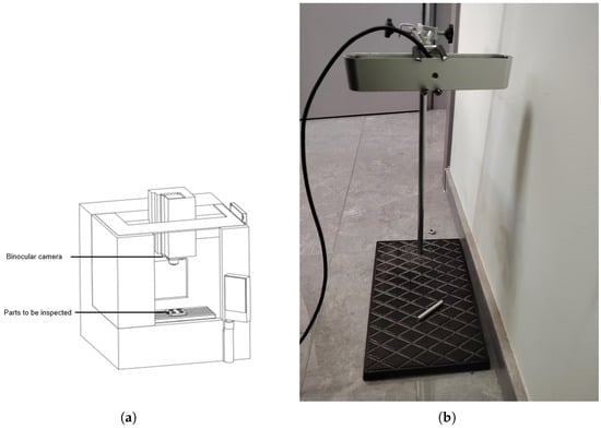
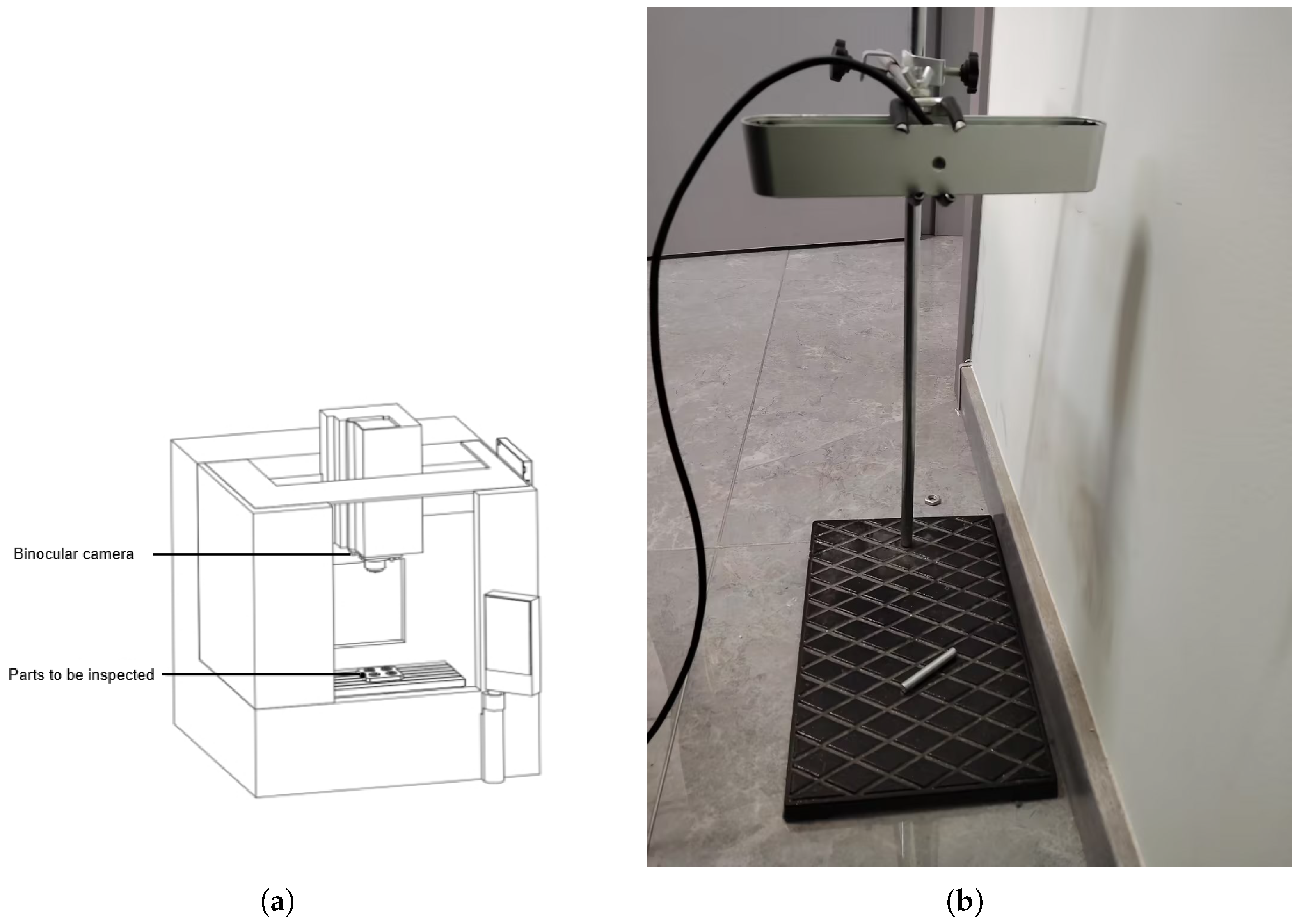
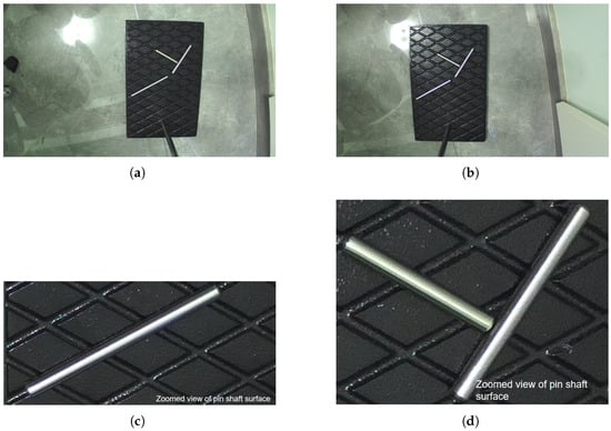
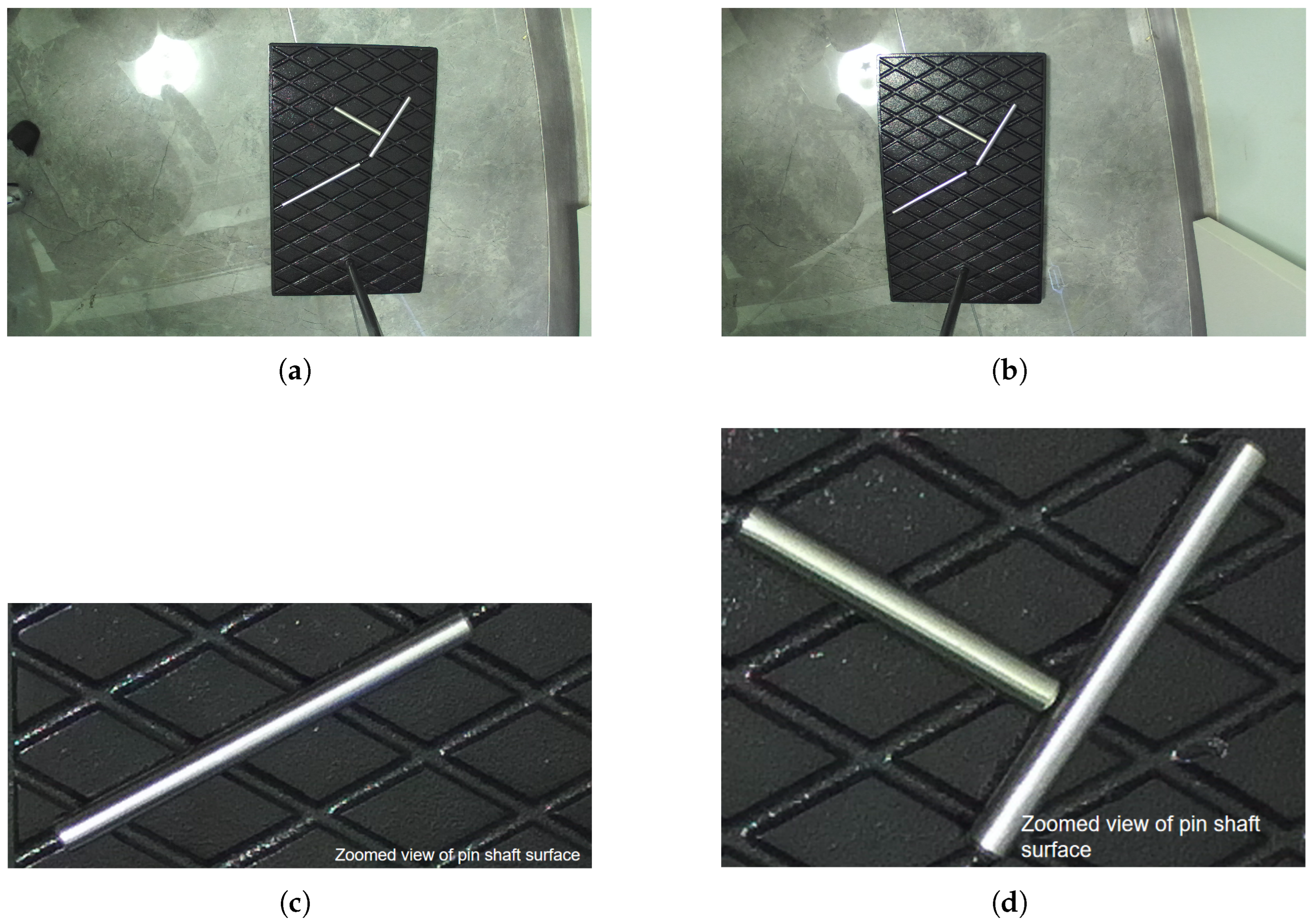
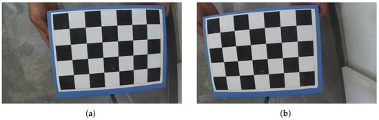
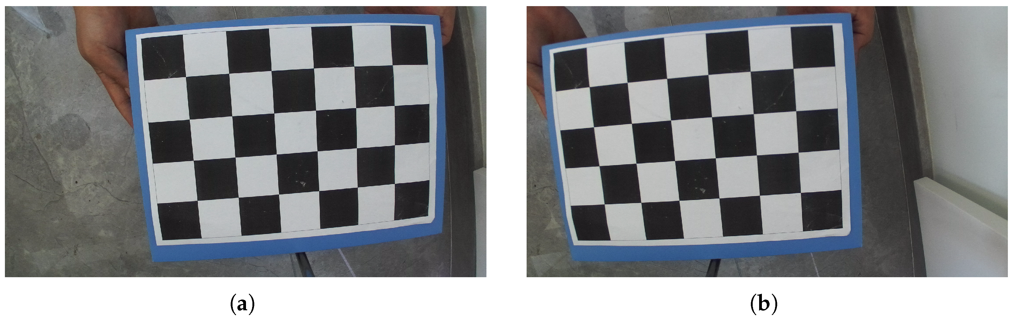


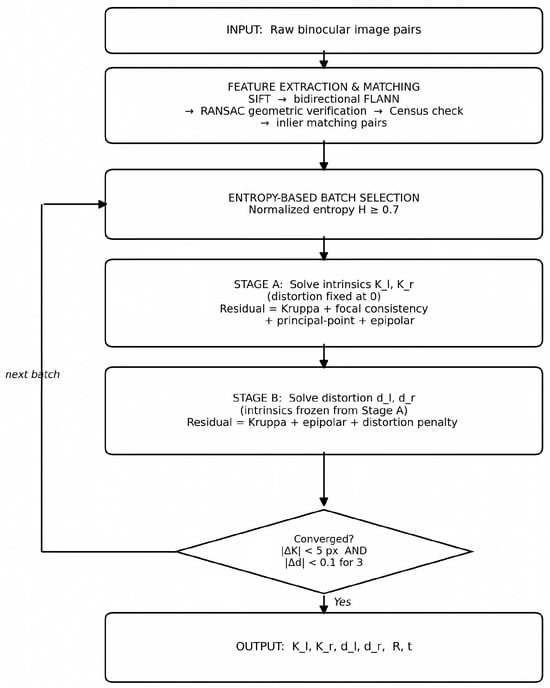
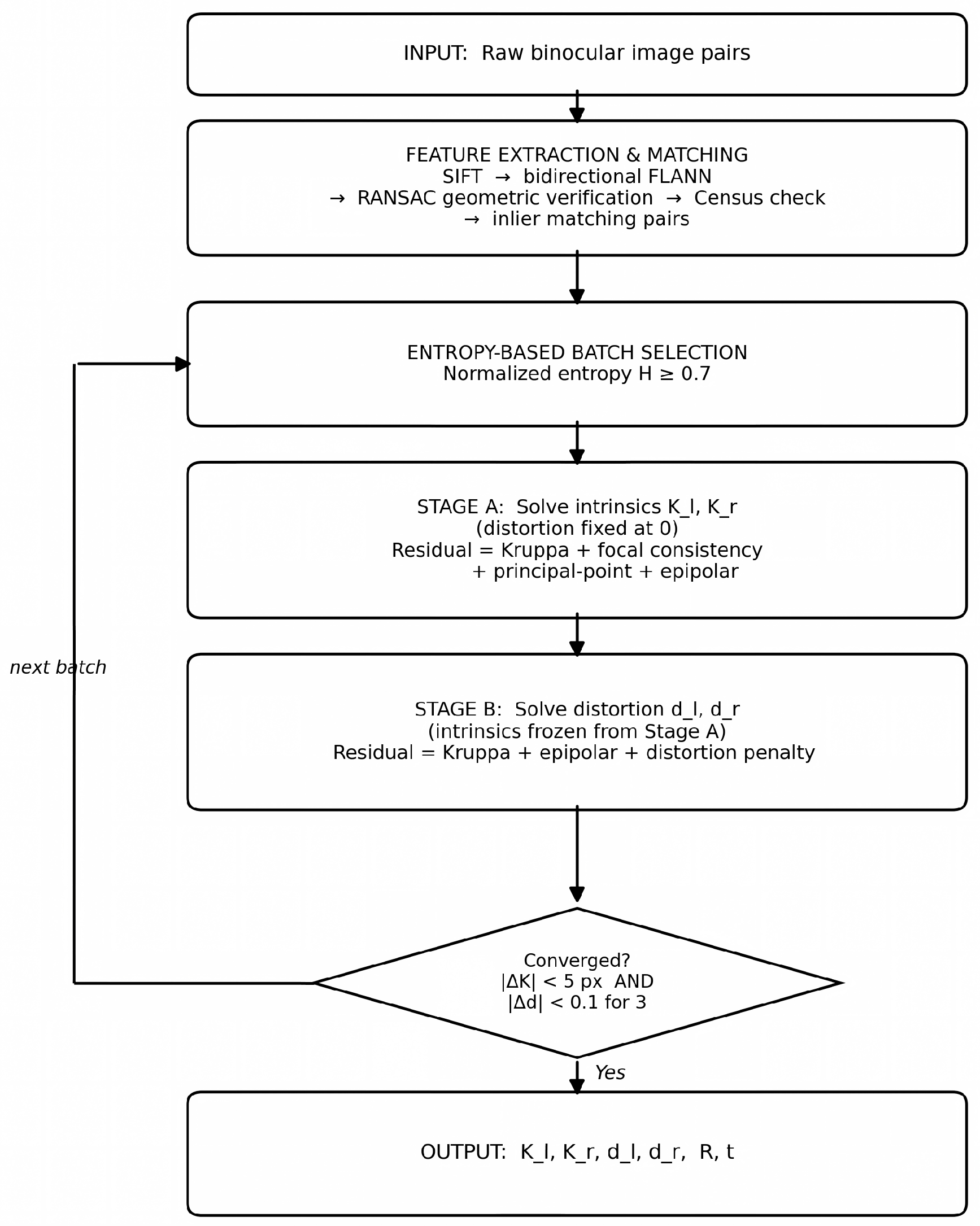
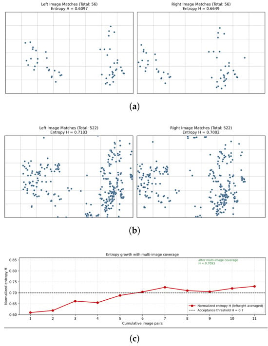
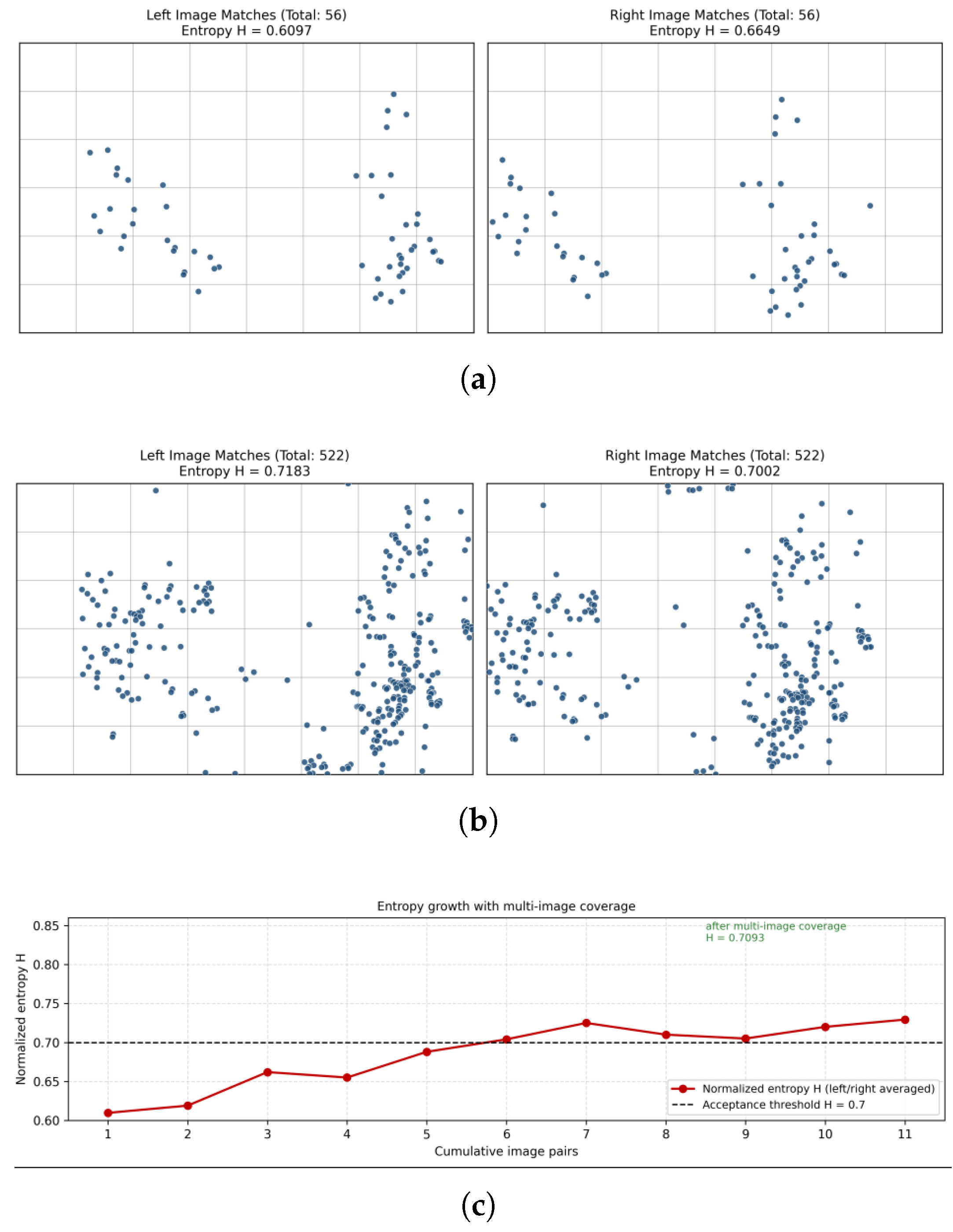
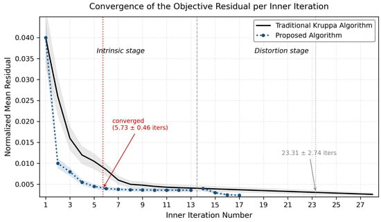
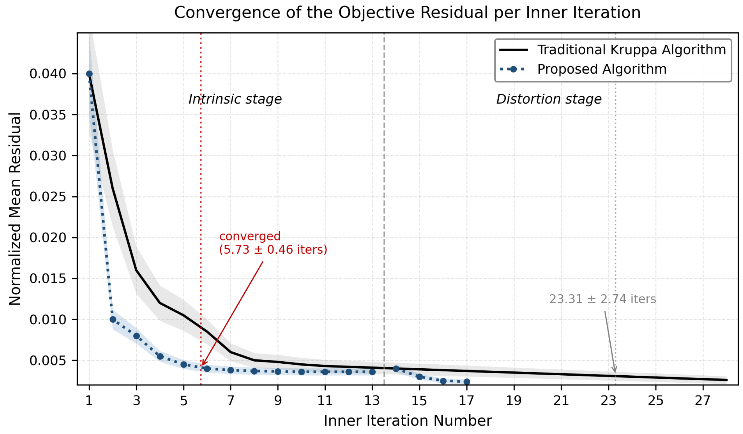
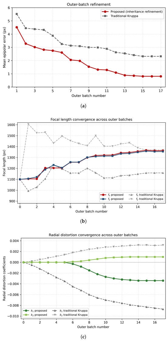
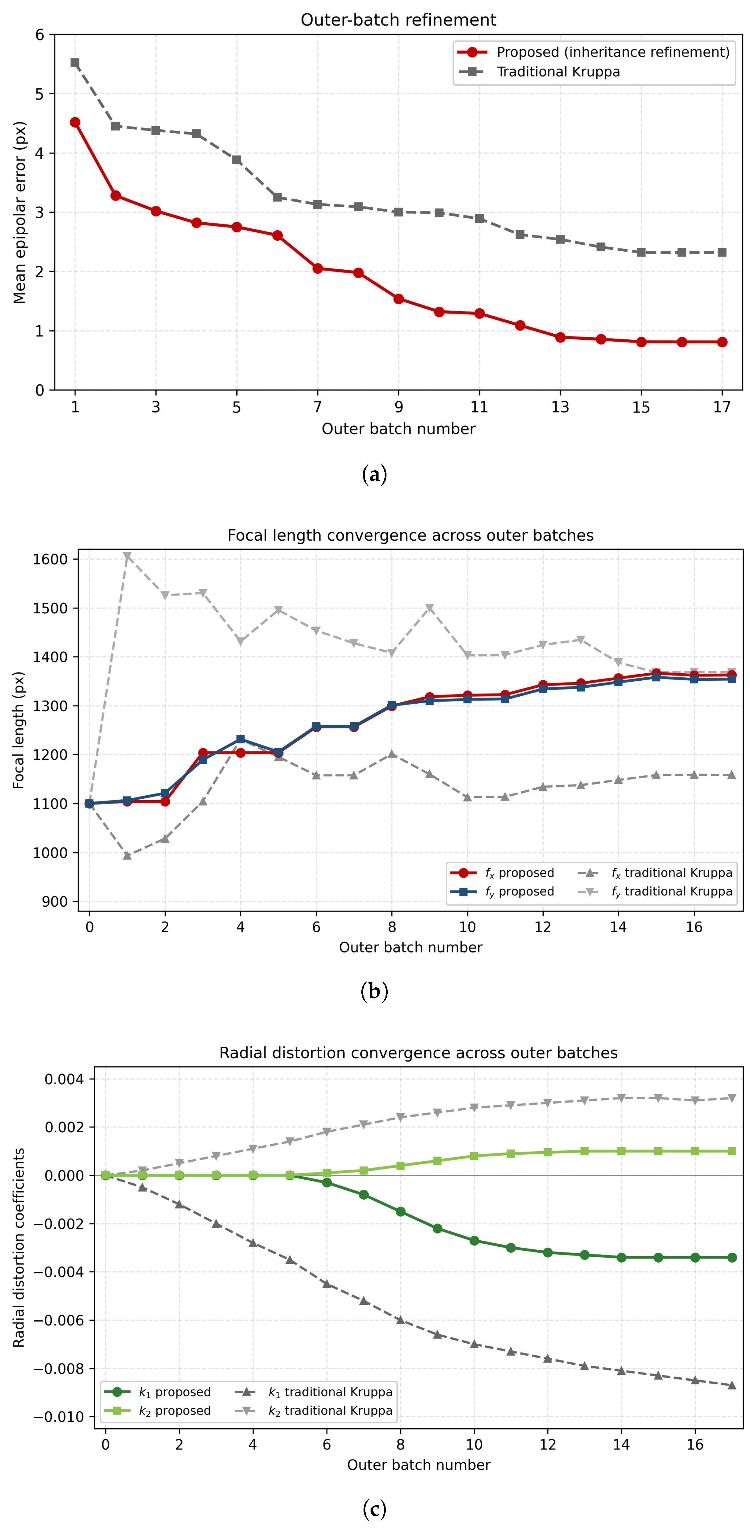
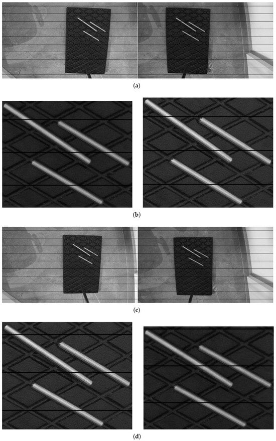
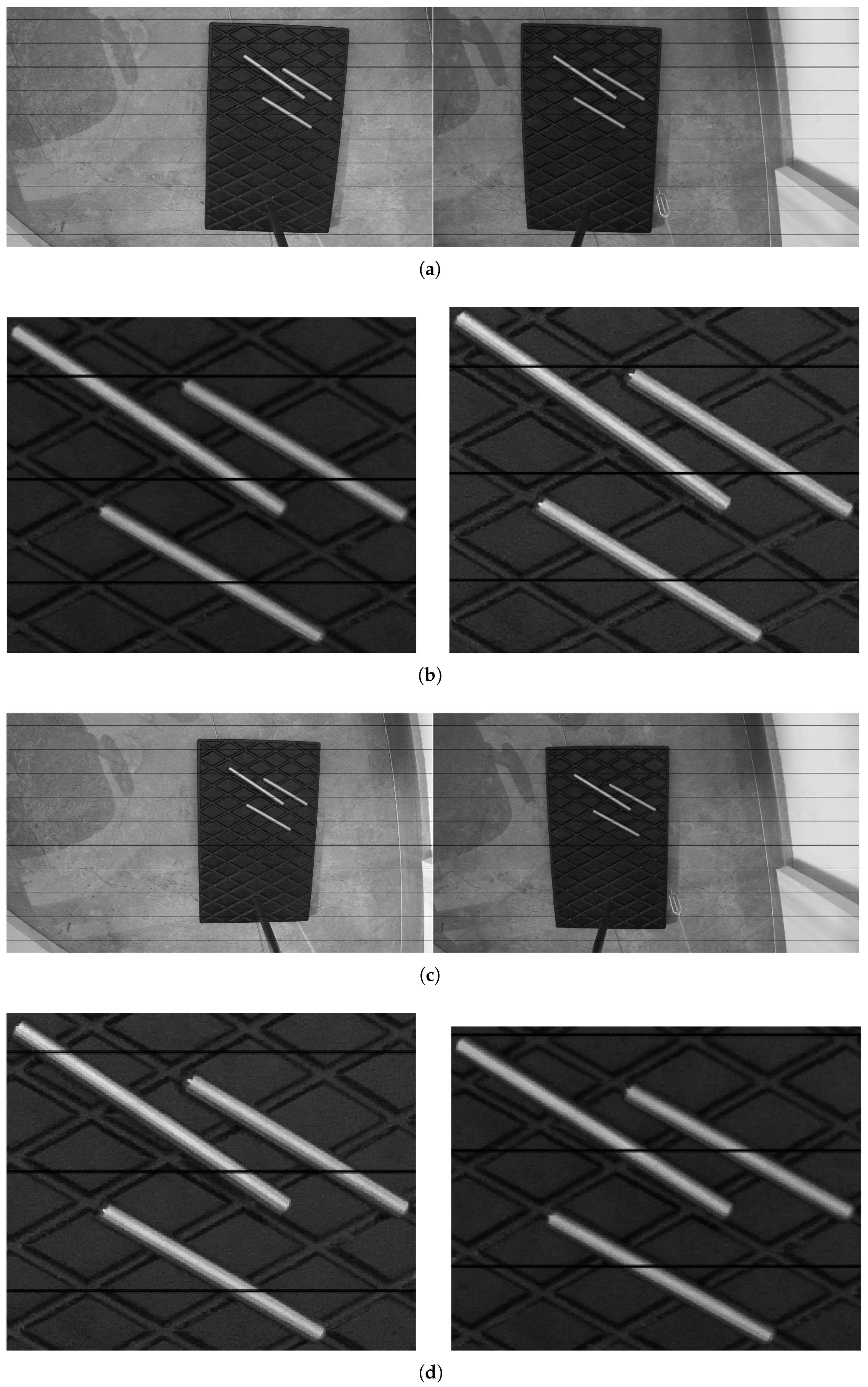
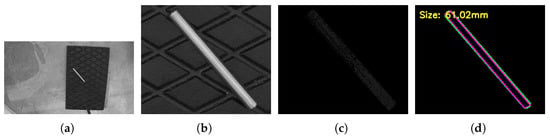
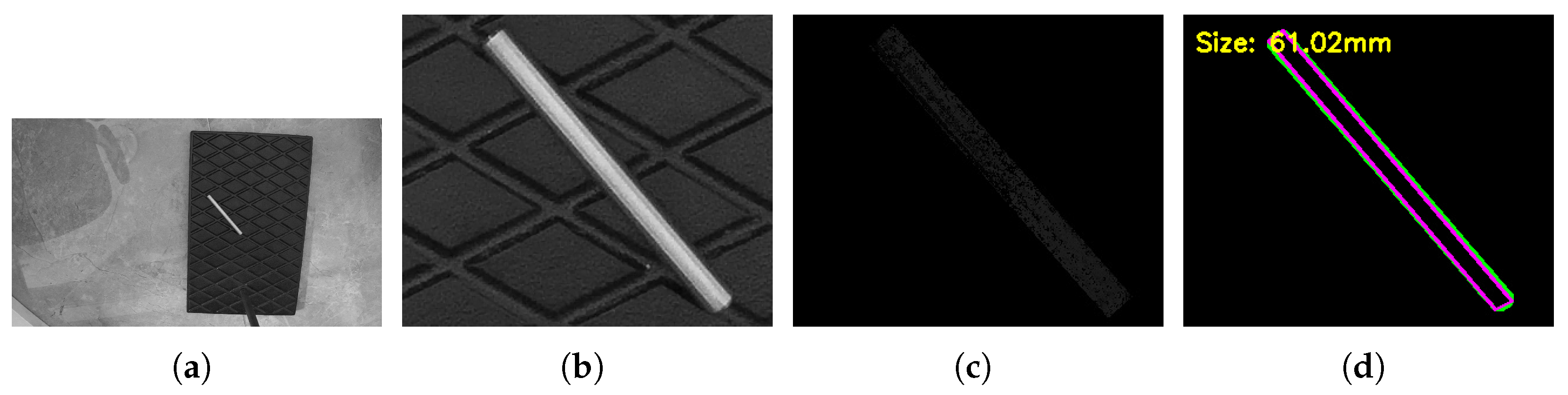
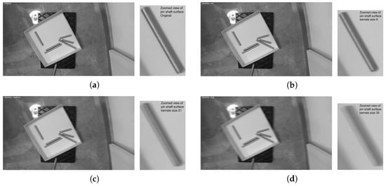
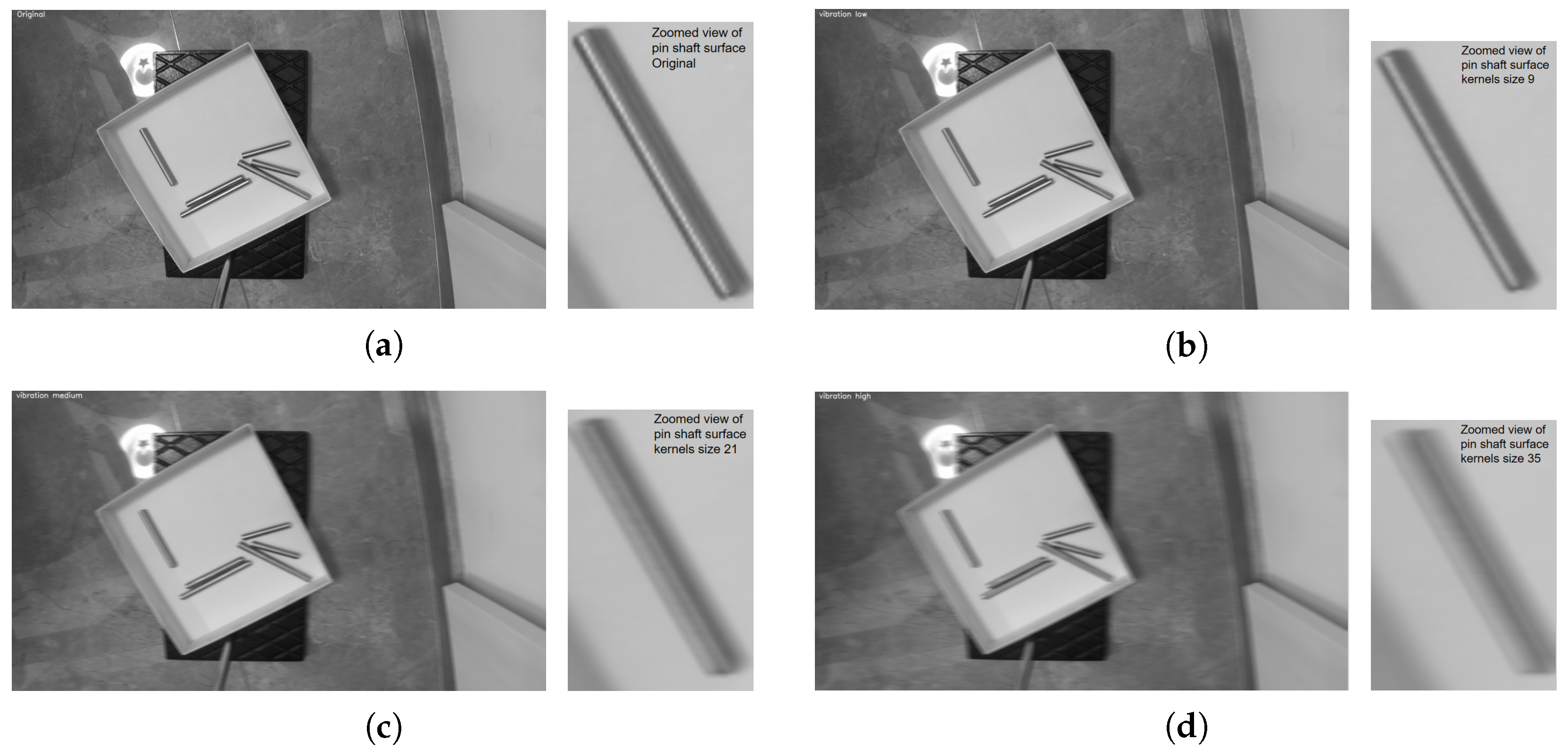
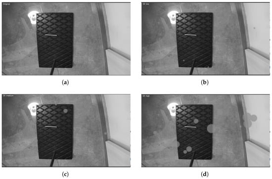
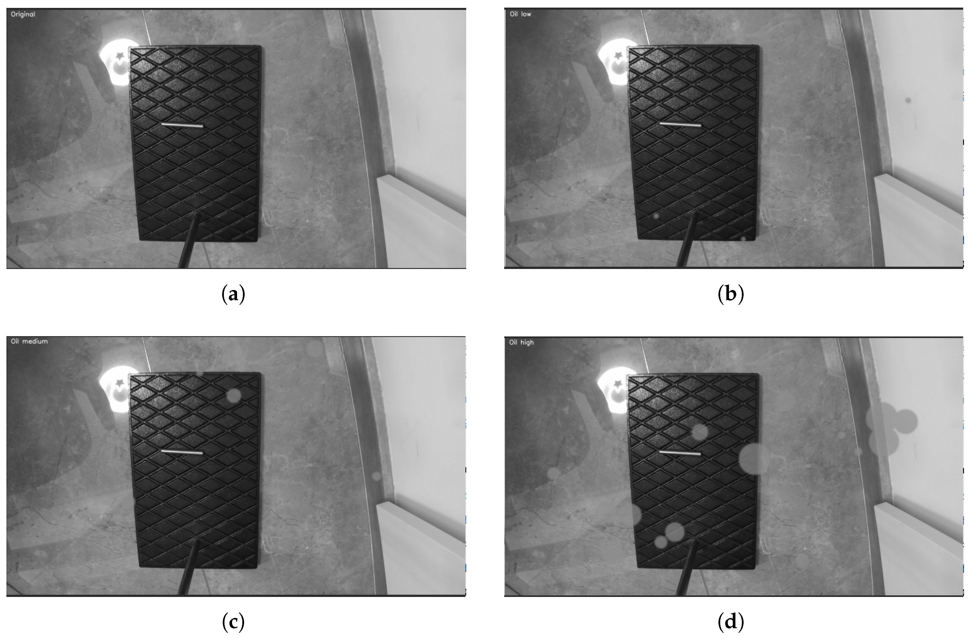

Disclaimer/Publisher’s Note: The statements, opinions and data contained in all publications are solely those of the individual author(s) and contributor(s) and not of MDPI and/or the editor(s). MDPI and/or the editor(s) disclaim responsibility for any injury to people or property resulting from any ideas, methods, instructions or products referred to in the content. |
© 2026 by the authors. Licensee MDPI, Basel, Switzerland. This article is an open access article distributed under the terms and conditions of the Creative Commons Attribution (CC BY) license.