Identifiability Limits of Discrete Axial Screw-Wear Diagnosis from Thermal and Electrical Process Signals During Soybean Extrusion

Featured Application

A campaign-adjusted rank and geometry audit can prevent process-signal differences from being interpreted as a spatially calibrated screw-wear map.

Abstract

This retrospective study audits whether a two-campaign soybean-extrusion archive supports section-specific inference in a linear geometry-associated signal model. The archive contains 3966 records (2091 worn and 1875 new) with four temperature and three phase-current channels. Descriptive statistics and complete recorded trajectories characterize the signal differences without treating time samples as independent experimental replicates. Eight section-associated predictor columns are assigned once per campaign from the available geometry documentation. With unrestricted campaign effects, these columns lie exactly in the campaign-indicator space: their added rank is zero and their coefficient nullity is eight per channel. Intercept-only adjustment retains at most one between-campaign contrast, whose physical cause cannot be isolated. An explicit reparameterization example illustrates identical fitted responses from different regression coefficients. The geometry audit reproduces source-cell formulas and establishes the discrete order 1–5–2–6–3–7–4–8, while identifying reversed endpoint labels, different percentage conventions, and absent measurement pairing and uncertainty documentation. These findings delimit inference for the specified archive and model; they do not establish a universal impossibility of thermal or electrical wear diagnosis. A reproducible audit sequence and maintenance decision criteria connect the results to mechanical engineering practice.

1. Introduction

The extrusion screw is a load-bearing and material-conveying component whose geometry governs transport, pressure generation, shear, and heat transfer. Wear changes flight clearance and can alter process capacity and drive loading; mechanical studies have modelled the effect of clearance growth on extruder performance and the evolution of screw-flight wear under operating conditions [1,2]. Experimental work on twin-screw machines has also shown that wear can be spatially concentrated by local force and gap geometry [3]. These results make screw wear a mechanical condition with potentially local consequences, but they do not imply that every process signal contains enough independent information to reconstruct a local wear map.

Signal-based studies have used pressure, torque, motor current, or multiple process sources to detect operating changes associated with wear. Ekielski et al. examined pressure and screw-load responses in food extrusion [4]; Danielak et al. used current signatures for wear detection [5]; Park et al. extracted degradation features from multi-source monitoring data [6]; and Durczak et al. reported non-invasive electrical condition assessment in an industrial extruder [7]. Spatially resolved process monitoring also has precedents, including monitoring the degree of fill in screw zones [8]. This article therefore does not claim to introduce spatial screw monitoring. It asks a narrower question: whether the particular soybean archive and its geometry records identify an eight-component axial wear profile after campaign differences are accounted for.

Condition monitoring commonly proceeds from sensor response to condition indicators, diagnosis, and maintenance decisions [9,10,11,12]. These stages answer different engineering questions. A statistical or classifier-based separation between two records may establish that the observed signals differ; it does not, by itself, identify which screw section caused the difference, quantify local wear, or establish a calibrated relation between a signal and a dimensional measurand. Confounding by campaign, material state, operating inputs, and sensor offsets matters because each can change the measured response.

Identifiability theory makes this distinction precise. A parameter is identifiable only when distinct parameter values cannot produce the same observations under the specified model and design. This principle has been developed for structural, parametric, and linear models, as well as for nonlinear dynamical systems [13,14,15,16,17,18]. In a linear design, projecting the regressors of interest off nuisance regressors yields a direct rank test; the Frisch–Waugh–Lovell results provide the relevant algebraic basis [19,20]. When the projected profile design has deficient rank, more observations along the same design pattern cannot recover the missing directions.

The contribution is an integrated, reproducible pre-modelling audit of the link between process records and section-level geometric targets. Established projection and rank theory are combined with source-cell metrological traceability, an explicit observational-equivalence example, and a decision table distinguishing record-level observations from section-specific maintenance claims. The algebra applies to any linear design whose candidate predictors are constant within unrestricted nuisance blocks, irrespective of machine type or block size. Its application and experimental evidence here remain specific to the soybean archive. RAPID names the organization of these established checks, not a new identifiability theorem or an independently validated wear estimator.

Table 1 positions the study alongside mechanical wear models and signal diagnostics. The following audit propositions specify the claims examined; H1 and H2 are consequences of the stated design assumptions, rather than independent statistical hypotheses tested against signal samples:

Table 1. Position of the present study relative to mechanical wear and process-diagnostic literature.

Study/Area	Measurement or Model Target	What the Work Establishes	Boundary Addressed Here
Klein [1]; Yang et al. [2]	Extruder performance and screw-flight wear mechanics	Wear and clearance have mechanical consequences; spatial wear laws can be modelled.	Does not establish profile identifiability from this archive.
Demirci et al. [3]	Local force and gap effects in twin-screw wear	Wear can be spatially concentrated; spatial wear work already exists.	Different machine and measurements; no claim of first spatial monitoring.
Ekielski et al. [4]; Danielak et al. [5]	Pressure, torque, and current signatures	Process signals can support wear-related condition detection.	Signal contrast is not an eight-section geometric estimate.
Park et al. [6]; Durczak et al. [7]	Multi-source degradation features and electrical monitoring	Operational data can support degradation monitoring and condition assessment.	Does not replace the present campaign-adjusted rank and metrology audit.
Taki et al. [8]	Spatially structured monitoring of screw fill	Screw-zone process monitoring is an established engineering direction.	Monitors process state, not this screw’s wear profile.
Present study	Rank, null space, and geometry documentation	Defines which profile directions are and are not supported by the two-campaign archive.	No signal-classification performance or millimetre calibration is claimed.

H1. 

In the linear audit model with unrestricted campaign effects, campaign-constant section predictors add no rank and their eight regression coefficient directions remain aliased.

H2. 

If campaign effects are reduced to a global intercept, the two campaign patterns support at most one profile-space contrast, leaving at least seven directions unresolved.

H3. 

The supplied documents establish discrete section order and reproducible worksheet arithmetic, but do not establish metric section positions, paired measurement locations, or eight interchangeable calibrated wear measurands.

The analysis uses the existing data as a bounded case study. It does not estimate a nonlinear process model, a wear profile in millimetres, or the causal effect of wear on any individual channel.

2. Materials and Methods

2.1. Data Sources and Experimental Unit

The sources comprise the process workbook, the eight-section geometry workbook, and the supplied screw drawing in PDF/JPG, provided in the Supplementary Materials. Records were retained when all seven signal cells were numeric and the material label identified STARY (worn) or NOWY (new), yielding 3966 records. Header, start-marker and blank rows were excluded; no smoothing, detrending, interpolation, resampling or outlier removal was applied. Both start markers specify a 6 mm die. The worn block was recorded on 27 July 2026 from 15:47:43.046 to 16:22:35.072 and the new block from 16:55:19.077 to 17:26:39.075. Timestamp spacing had a median of 1.000 s in both blocks; ranges were 0.025–4.932 s and 0.985–4.017 s, respectively. The inter-block gap was 1964.005 s. The gap documents elapsed time only; its operational cause is unavailable. No independent repeated campaign was identified.

Synchronized rotational speed, feed rate, moisture, pressure, torque and throughput histories are absent. The files do not document screw service hours, replacement of other components, sensor reinstallation or calibration, raw-material batch identity, or a restart log. Sensor positions, instrument resolution and calibration uncertainty are not established by these files. The absence of metadata prevents demonstration that the campaigns are otherwise comparable. Channel values are reproduced in their recorded scale; units and sensor calibration are not independently verified from the archive.

The time rows are observations within two process campaigns, not independent screw-level replicates. The distinction between sampling density and experimental replication is central to the analysis and follows standard cautions about pseudoreplication and nested observations [21,22]. Table 2 summarizes the audited archive.

Table 2. Inventory of the analyzed process and geometry records.

Audit Item	Observed in the Supplied Files
Valid process records	3966 rows with an old/worn or new condition label.
Worn-screw campaign	2091 records; one contiguous labeled block.
New-screw campaign	1875 records; one contiguous labeled block.
Campaign replication	Two condition campaigns in sequence; no independent repeated trajectory was identified.
Temperature channels	Four channels (Temp_1–Temp_4).
Electrical channels	Three phase-current channels (L1–L3).
Sampling interval	Approximately 1 s; timestamps span 27 July 2026.
Unobserved process inputs	No synchronized speed, feed, moisture, pressure, torque, or throughput series in the inspected workbook.
Geometry workbook	Eight discrete sections: four flight sections and four restriction rings.

2.2. Design Representation and Target Profile

The response matrix contains the seven channels, and the campaign matrix has two indicator columns. In Equation (1), W denotes an assigned section-associated predictor design, not eight independently observed temporal wear histories, a process Jacobian, or the unknown physical wear profile. Each row receives the same eight geometry-associated entries as all other rows from its campaign. B contains signal-regression coefficients for these assigned predictors; its entries are not section wear in millimetres. This distinction separates limitations of the selected linear model from limitations of the measurement archive. Table 3 defines the notation.

Y = ZA + WB + E

(1)

Table 3. Legend of mathematical symbols, indices, and geometric parameters used in the manuscript.

Symbol/Term	Dimension/Unit	Definition and Role
n,p,q	n = 3966; p = 7; q = 8	Numbers of labeled observations, measured response channels, and discrete screw-section coordinates.
Y	n × p	Response matrix containing Temp_1–Temp_4 and the three phase-current channels L1–L3.
Δa	p-vector	Worn-minus-new difference between the two campaign-effect coefficient rows of A; this nuisance contrast remains after intercept-only projection in Equation (16).
Z,W,C0	n × 2; n × 8; 2 × 8	Campaign-indicator matrix; candidate section-profile design; and mapping satisfying W = ZC0 for the observed campaign pattern.
A,B,E	2 × p; 8 × p; n × p	Campaign-effect coefficients, candidate section-profile coefficients, and residual matrix in the design-audit model.
π,j	π = (1, 5, 2, 6, 3, 7, 4, 8); j = section code	Discrete axial ordering and section index. The sequence provides order only, not millimetre coordinates.
MZ	n × n	Ordinary least-squares residual-maker that projects observations off the campaign-indicator space.
DZ,ΔrZ	n × 8; scalar	Campaign-residualized profile design and incremental design rank contributed by the profile columns.
GZ,ker(DZ),EB	8 × 8; subspaces of R8	Profile Gram matrix; unresolved coefficient directions; and estimable linear combinations of profile coefficients, respectively.
Ω,MZ,Ω	n × n; n × n	Positive-definite observation covariance matrix and the corresponding generalized residual-maker. The inverse Ω−1 is the precision matrix used in weighted projection.
1n,M1,D1	n; n × n; n × 8	All-ones vector; intercept residual-maker $M_1=I_n-{\displaystyle \frac{1}{n}}{\mathbf{1}}_n{\mathbf{1}}_n^{\mathrm{\top }}$; and intercept-residualized profile design D1 = M1W.
s,sc,c,d	n-vectors; 8-vectors	Binary indicator (1 for worn, 0 for new), its centered version, the new-campaign section pattern, and the worn-minus-new section difference, respectively. The centered squared norm is 988.56.
A*,B*,H	2 × p; 8 × p; 8 × p	Observationally equivalent coefficient representation and arbitrary shift H used to demonstrate campaign/profile aliasing.
X7,I7,⊗	7n × 70; 7 × 7	Block-diagonal extension across the seven response channels; identity matrix; and Kronecker product.
$\begin{array}{c}\mathrm{rank}\left(\cdot \right),\ker \left(\cdot \right),\\ \dim \left(\cdot \right),{\left(\cdot \right)}^{\mathrm{\top }}\end{array}$	operators	Rank, null space, vector-space dimension, and transpose.
dN,j,dW,j	mm	New-screw and worn-screw diameters for section j; flight sections have source-labelled maximum/minimum readings, whereas ring sections have one recorded diameter.
wj,min,wj,max,wj,ring	mm	Workbook-derived diameter reductions for flight endpoints and restriction rings, as defined in Equations (21) and (22).
rj,min,rj,max	dimensionless	Dimensionless workbook ratios for flight endpoints. The results section displays 100 times these ratios in percent; the second ratio uses a different numerator from the millimetre maximum-reduction formula in Equation (21).
Z+,W+	prospective matrices	Campaign and profile designs for a future experiment; + marks the proposed design, for which all eight profile directions require full residualized rank.

Equation (2) is an assumption-supported design identity: there are only two independently documented geometry patterns, each assigned to one complete campaign. No record independently links a response channel to one screw section. To make the numerical representation transparent, the reproducibility example uses the source-labelled maximum flight diameter or single ring diameter in each section, ordered by Equation (3). New-campaign entries are 65.48, 64.01, 64.48, 64.61, 64.51, 64.82, 64.38 and 64.312 mm; worn-campaign entries are 64.43, 62.94, 64.35, 63.36, 63.85, 63.91, 64.30 and 63.55 mm. These are recorded diameter descriptors, not a corrected or homogeneous wear target. The exact aliasing result holds for any alternative eight-entry encoding constant within the same campaign blocks, including one using documented reductions; it is not dependent on this choice of numeric encoding.

W = ZC₀,  rank(Z) = 2

(2)

π = (1,5,2,6,3,7,4,8)

(3)

2.3. Campaign-Adjusted Rank and Estimable Profile Combinations

The campaign-adjusted projection removes the column space of the campaign indicators. Equation (4) defines the ordinary least-squares residual-maker. The residualized profile design in Equation (5) is the object whose rank determines whether any profile direction remains after campaign adjustment. The incremental-rank identity in Equation (6) is the primary test.

$$M_Z=I_n-Z{\left(Z^{\mathrm{\top }}Z\right)}^{-1}{Z}^{\mathrm{\top }}$$

(4)

D_Z = M_ZW

(5)

Δr_Z = rank([Z W]) − rank(Z) = rank(M_ZW)

(6)

The profile Gram matrix in Equation (7) summarizes the same residualized design geometry. Its null space is the set of profile perturbations that leave the fitted campaign-adjusted design unchanged. Equation (8) states the full eight-dimensional null space expected if all profile columns are aliased.

$$G_Z=W^{\mathrm{\top }}{M}_{Z}W=D_Z^{\mathrm{\top }}{D}_Z$$

(7)

ker(D_Z) = R⁸,  dim ker(D_Z) = 8

(8)

A direct invariance argument clarifies the consequence. For any eight-by-channel matrix of perturbations, the campaign coefficients can absorb the corresponding profile change when Equation (2) holds. Equation (9) gives this observationally equivalent reparameterization. Accordingly, only linear combinations lying in the row space of the residualized profile design can be estimable, as stated in Equation (10).

A^⋆ = A − C₀H, B^⋆ = B + H, H∈R^8×p

(9)

E_B = row(D_Z)

(10)

To show that temporal correlation does not rescue exact aliasing, a generalized least-squares projection was also written for any positive-definite observation covariance matrix. Equations (11) and (12) show that when the profile columns are exactly contained in the campaign space, the weighted residualized profile design and its weighted Gram matrix are still zero. This is a design result; it is not a full Fisher information matrix for a nonlinear extrusion model.

$$M_{Z,\Omega }=I_n-Z{\left(Z^{\mathrm{\top }}{\Omega }^{-1}Z\right)}^{-1}{Z}^{\mathrm{\top }}{\Omega }^{-1}$$

(11)

M_Z,ΩW = 0,  W^⊤Ω⁻¹M_Z,ΩW = 0_8×8

(12)

2.4. Intercept-Only Sensitivity and Multichannel Extension

A sensitivity analysis projected off only the global intercept, leaving differences between the two campaigns in the response. The matrix M₁ is defined in Table 3. Set the binary indicator to one for worn-campaign rows and zero for new-campaign rows; c is the new-campaign section pattern and d is the worn-minus-new difference. Equation (13) gives the record counts, while Equation (14) defines the intercept-residualized profile design and its outer-product form.

n_worn = 2091, n_new = 1875, n = 3966

(13)

$$\begin{array}{ll}W& ={\mathbf{1}}_n{c}^{\mathrm{\top }}+s{d}^{\mathrm{\top }},\\ D_1& =M_{1}W=s_c{d}^{\mathrm{\top }}, s_c=M_{1}s\end{array}$$

(14)

The design in Equation (14) has rank at most one and has rank one when the section-pattern difference is nonzero, as stated in Equation (15). Applying the intercept projection to Equation (1) also retains the difference between the two rows of the campaign-effect matrix. Equation (16) displays both the campaign nuisance contrast and the candidate profile term in the observed response. The indicator norm in Equation (17) measures design scale; it is not an effect size, test statistic, uncertainty estimate, or Fisher information.

rank(D₁) = 1

(15)

$$\begin{array}{ll}\Delta a^{\mathrm{\top }}& =A_{\mathrm{worn},:}-A_{\mathrm{new},:},\\ M_{1}Y& =s_c\left(\Delta a^{\mathrm{\top }}+d^{\mathrm{\top }}B\right)+M_{1}E\end{array}$$

(16)

$$s_c^{\mathrm{\top }}{s}_c={\displaystyle \frac{n_{\mathrm{worn}}{n}_{\mathrm{new}}}{n}}=988.56$$

(17)

Equation (18) gives the unresolved coefficient dimension for a nonzero campaign-pattern difference. Equation (19) repeats the design in seven separate coefficient blocks; Equation (20) is a bookkeeping extension demonstrating that separate channel fits inherit the defect. It is not a joint physical model of electrical and thermal responses. Cross-channel covariance may affect uncertainty but cannot change exact column containment in this formulation. A model with known shared physical constraints or independently measured spatial sensitivities would require a separate identifiability analysis.

dim ker(D₁) = 8 − rank(D₁) = 7

(18)

X₇ = I₇⊗[Z W]

(19)

$$\begin{array}{cc}\hfill \mathrm{rank}\left(X_7\right)& =7\mathrm{rank}\left(\left[Z\hspace{0.33em}W\right]\right)=14,\hfill \\ \hfill \dim \hspace{0.17em}\ker \left(X_7\right)& =70-14=56\hfill \end{array}$$

(20)

2.5. Geometry and Metrological Audit

Sections 1–4 have source-labelled maximum/minimum diameters; sections 5–8 have one diameter each. Equations (21)–(23) reproduce the worksheet arithmetic. They do not establish matched pre/post-wear measurements, radial material loss, or calibrated wear. Each flight reduction uses the same new maximum reading as reference, whereas the maximum percentage uses the new minimum reading. The results section separately reports the four readings and the source-cell operands with independent recalculations. Unknown physical pairing is not repaired by relabelling or sorting the readings.

$$w_{j,\min }=d_{\mathrm{N},j}^{\max }-d_{\mathrm{W},j}^{\max }, w_{j,\max }=d_{\mathrm{N},j}^{\max }-d_{\mathrm{W},j}^{\min }$$

(21)

w_j,ring = d_N,j − d_W,j

(22)

$$r_{j,\min }={\displaystyle \frac{d_{\mathrm{N},j}^{\max }-d_{\mathrm{W},j}^{\max }}{d_{\mathrm{N},j}^{\max }}}, r_{j,\max }={\displaystyle \frac{d_{\mathrm{N},j}^{\min }-d_{\mathrm{W},j}^{\min }}{d_{\mathrm{N},j}^{\min }}}$$

(23)

The audit checked section labels, diameter endpoint order, formula consistency, dimensional units, stated axial coordinates, measurement datums, and reported uncertainty. This follows the metrological distinction between a numerical indication and a defined measurand with traceability and uncertainty [23,24]. The geometry audit was used to determine which labels can be interpreted, not to infer unrecorded coordinates or uncertainty intervals.

For Sections 1–4, numerical reproduction uses cells B–I in rows 6–9 of sheet screw wear; rings occupy rows 10–13. Formula text and saved results are retained in the supplement. Cells E10–E12 contain percentage-type formulas under the worn-minimum diameter header, but refer to blank C cells and return empty strings. They are formula artefacts, not additional diameter measurements. The drawing identifies sections but does not show the angular direction, contact surfaces or matched diameter measurement datums. It therefore supports discrete order only. No instrument, repeatability, manufacturing tolerance or uncertainty record is available.

2.6. Audit Workflow, Numerical Scope, and Future Design

RAPID comprises five reproducible steps: reconstruct the observation-to-geometry assignment; adjust for explicitly specified nuisance terms; project candidate predictors; inspect exact rank, null space and observational equivalence; and document geometry provenance and permitted decisions. Inputs are the label sequence, candidate predictor assignment and dimensional records. Outputs are an estimability statement conditional on the model, a traceable arithmetic audit and a maintenance inference boundary. The exact result follows from block-constant assignment and needs no floating-point tolerance. Numerical computations in the supplement illustrate this identity using a documented diameter encoding.

No nonlinear process model, synchronized operating-input histories, or model sensitivities with respect to section wear were available in the inspected archive. Therefore, no nonlinear Jacobian, likelihood-based Fisher information matrix, wear calibration, or uncertainty interval for an eight-element profile was calculated. A future design capable of identifying all eight profile components must satisfy the full-rank condition in Equation (24); practical precision would additionally depend on singular values, process noise, measurement uncertainty, and independent screw-level replication. Optimal experiment design provides established tools for selecting such operating conditions [25].

$$\mathrm{rank}\left(M_{Z^{+}}{W}^{+}\right)=8$$

(24)

2.7. Descriptive Signal Characterization and Illustrative Equivalence

The supplementary computations were independently re-executed during proofreading using Python 3.12.14, NumPy 2.3.5, openpyxl 3.1.5 and Matplotlib 3.10.8. For each channel and campaign, the number of records, mean, sample standard deviation, median, quartiles and range were calculated on all retained readings. Lag-one correlation describes adjacent records and is not interpreted as a stationary-process parameter. Complete trajectories are plotted against elapsed time within each campaign. No p-values, population confidence intervals or classifier performance are reported because the design contains only one campaign per condition and the records include substantial trends. The synthetic coefficient example applies Equation (9) to the transparent diameter encoding scaled by 65 mm for numerical convenience; it illustrates linear reparameterization only and does not simulate screw physics or add experimental observations.

Generative AI (ChatGPT, OpenAI; the exact model identifier was not retained) assisted drafting, organization, language editing and development of analysis code. The authors reviewed the text and computational outputs and retain responsibility for the work. The explicitly labelled illustrative coefficients are mathematical examples; no synthetic experimental measurements were introduced.

3. Results

3.1. Data Structure and Replication

The selection rule retained 2091 worn and 1875 new records from two contiguous blocks. Table 2 summarizes the available evidence. Start-marker rows identify the same nominal 6 mm die, but the approximately 32.7 min gap and unrecorded operating inputs prevent verification of otherwise equivalent conditions. Temporal density does not provide independent screw or campaign replication.

3.2. Exact Aliasing After Campaign Adjustment

For the campaign-constant predictor assignment in Section 2.2, the campaign-only design has rank two and the augmented design also has rank two. Equation (6) gives zero added profile-design rank. Equation (8) leaves eight regression coefficient directions unresolved per channel. This establishes non-estimability in Equation (1); it does not estimate the eight physical section wear values or demonstrate non-identifiability of every possible physical extrusion model.

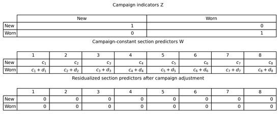
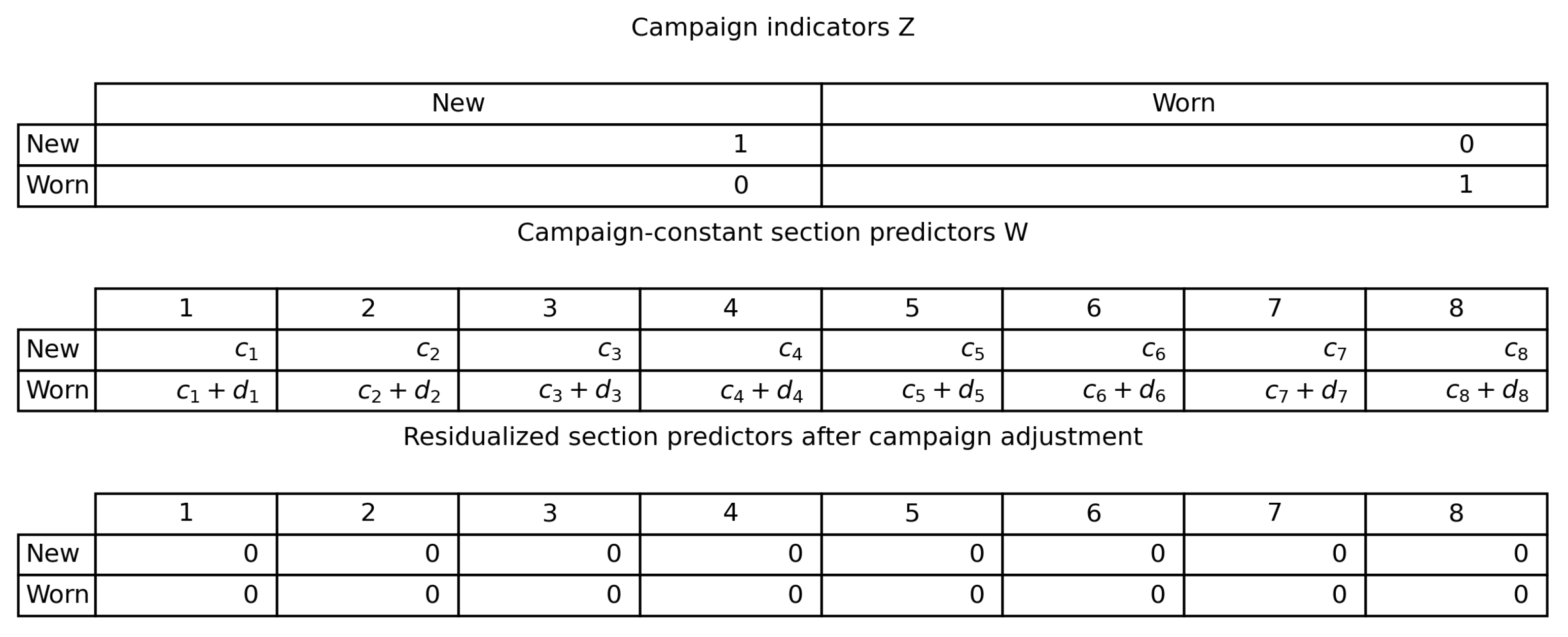
Table 4 reports the rank results for both nuisance specifications and for the seven-channel extension. Figure 1 shows the design geometry: the profile columns reproduce combinations of the campaign indicators. The identity is exact at the design level and is not a consequence of near-collinearity, an arbitrary numerical tolerance, or insufficiently dense sampling.

Table 4. Design rank and unresolved profile dimensions under alternative nuisance structures.

Nuisance Structure	Profile Terms	Total Coefficients	Design Rank	Added Profile Rank	Profile Nullity
Two campaign indicators	8 per channel	10 per channel	2	0	8 per channel
Global intercept only	8 per channel	9 per channel	2	1	7 per channel
Two campaigns; seven separate channels	56 across channels	70	14	0	56 across channels

Nullity refers to the kernel of the profile design after projection from the stated nuisance space. The seven-channel row is the block-diagonal extension of the same design, not seven independent process campaigns.

Figure 1. The eight profile columns lie within the space spanned by the campaign indicators; consequently, their campaign-residualized design is exactly zero.

3.3. Intercept-Only Contrast and Seven-Channel Rank

For the documented numeric example, the two diameter patterns differ, so the intercept-residualized predictor design has rank one under Equation (15), leaving seven unresolved coefficient directions under Equation (18). Equation (16) retains both the campaign nuisance contrast and the predictor contribution. Removing campaign adjustment therefore reallocates a between-record difference without identifying its physical cause; this is sensitivity to nuisance specification, not an alternative wear-profile estimate.

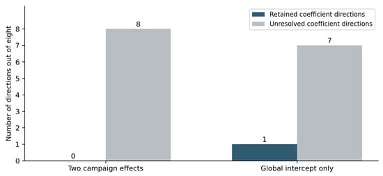
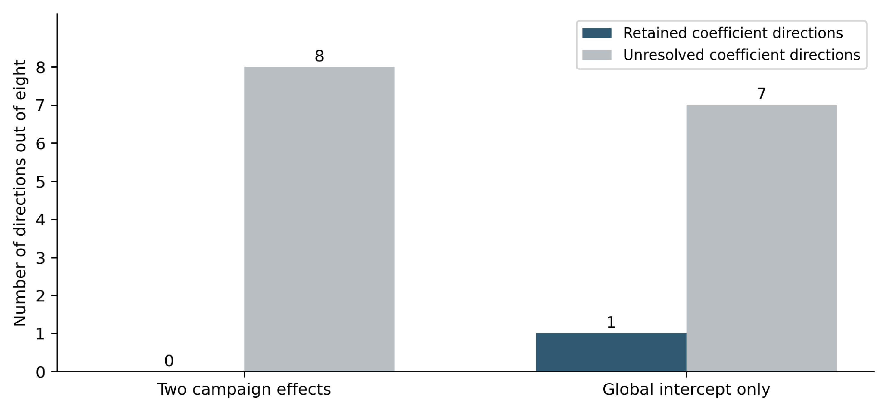
The centered indicator scale in Equation (17) was 988.56. This value describes the number and balance of records contributing to the binary contrast. It does not provide an estimate of profile precision or evidence that wear caused the observed record difference. Figure 2 summarizes how rank and profile nullity change under the two nuisance specifications.

Figure 2. Exact rank sensitivity for the documented nonzero diameter-pattern difference. Intercept-only adjustment retains one between-campaign coefficient direction and seven unresolved directions; unrestricted campaign adjustment leaves all eight unresolved. The retained contrast includes campaign effects and is not a wear estimate.

The block-diagonal extension contains 70 coefficients, has rank 14 and has coefficient nullity 56, as in Equation (20). This confirms the defect in seven separate channel fits and adds no empirical validation. It does not evaluate shared physical sensitivities across channels; those are not documented in the archive.

3.4. Geometry Workbook Audit

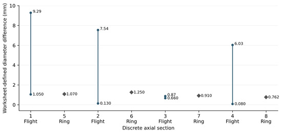
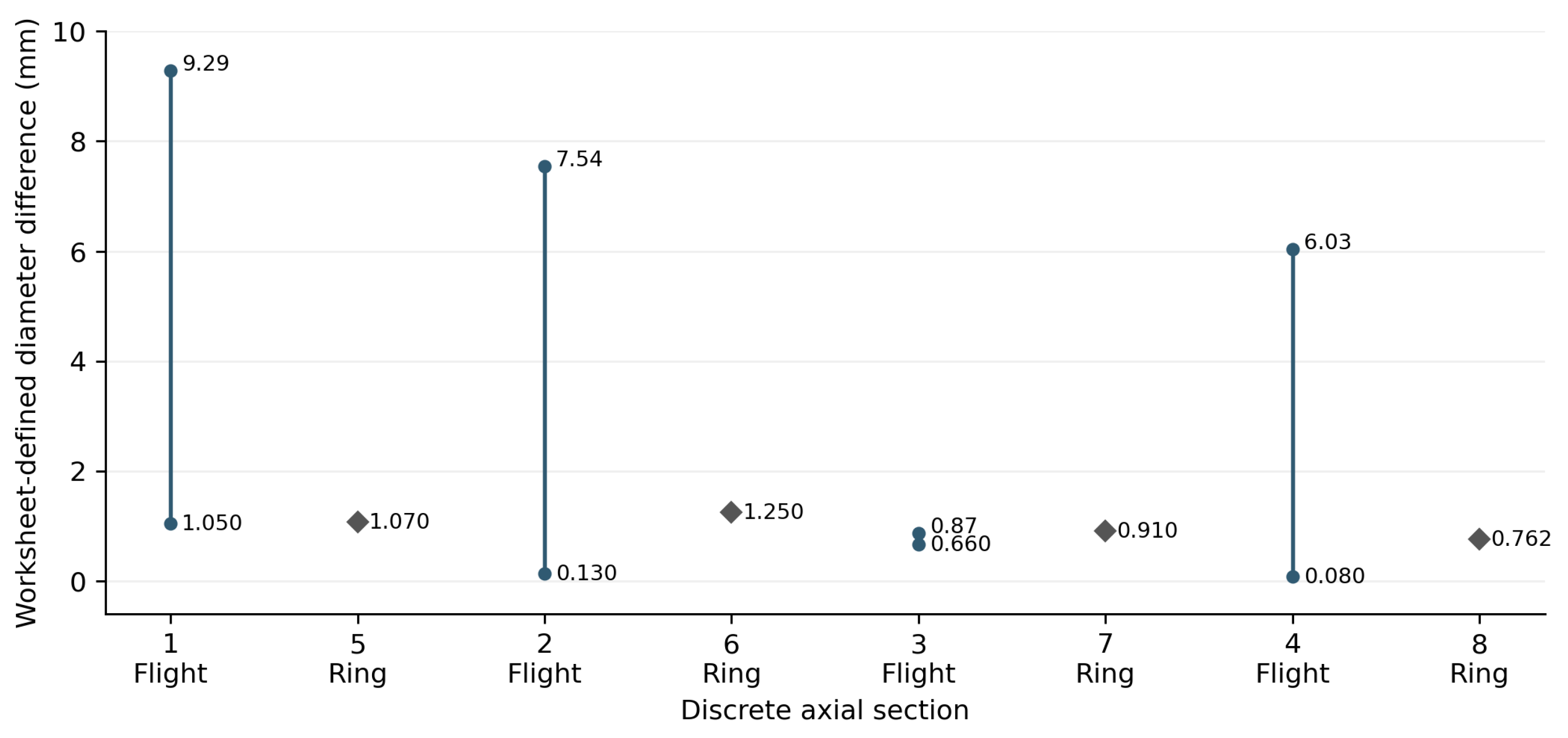
The drawing establishes order 1–5–2–6–3–7–4–8. Table 5 presents readings without compressing them into apparent matched pairs. Figure 3 plots the workbook-derived dimensional differences. These differences are not uncertainty intervals or evidence of a calibrated section wear vector.

Table 5. Source-labelled diameter readings in discrete axial order. Maximum/minimum labels are retained as recorded; empty ring endpoints are not zero.

Section	Element	New Max/Single (mm)	New Min (mm)	Worn Max/Single (mm)	Worn Min (mm)	Source Row
1	Flight	65.48	65.02	64.43	56.19	6
5	Ring	64.01	—	62.94	—	10
2	Flight	64.48	65.61	64.35	56.94	7
6	Ring	64.61	—	63.36	—	11
3	Flight	64.51	64.41	63.85	63.64	8
7	Ring	64.82	—	63.91	—	12
4	Flight	64.38	64.43	64.3	58.35	9
8	Ring	64.312	—	63.55	—	13

Source rows refer to sheet screw wear. In Sections 2 and 4, the new minimum exceeds the new maximum; the readings have not been reordered. Their physical measurement pairing is undocumented. The subsequent arithmetic audit reports the reproducible arithmetic, which must not be interpreted as metrologically verified material loss.

Figure 3. Geometry audit by discrete axial section, distinguishing flight endpoint pairs from single-valued restriction-ring measurements. The plotted ordinate is the workbook-derived diameter reduction defined in Equations (21) and (22).

The drawing labels overall diameters of 64.39 mm and 64.28 mm, compared with source-labelled Section 4 maximum diameters of 64.38 mm and 64.30 mm. The numerical differences are 0.01 and 0.02 mm. These are documentation comparisons, not established matched measurements. Without common datums, tolerances and uncertainty, their significance and origin cannot be determined; the differences alone do not prove measurement error.

3.5. Recorded Signal Variability

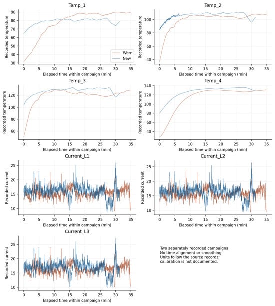
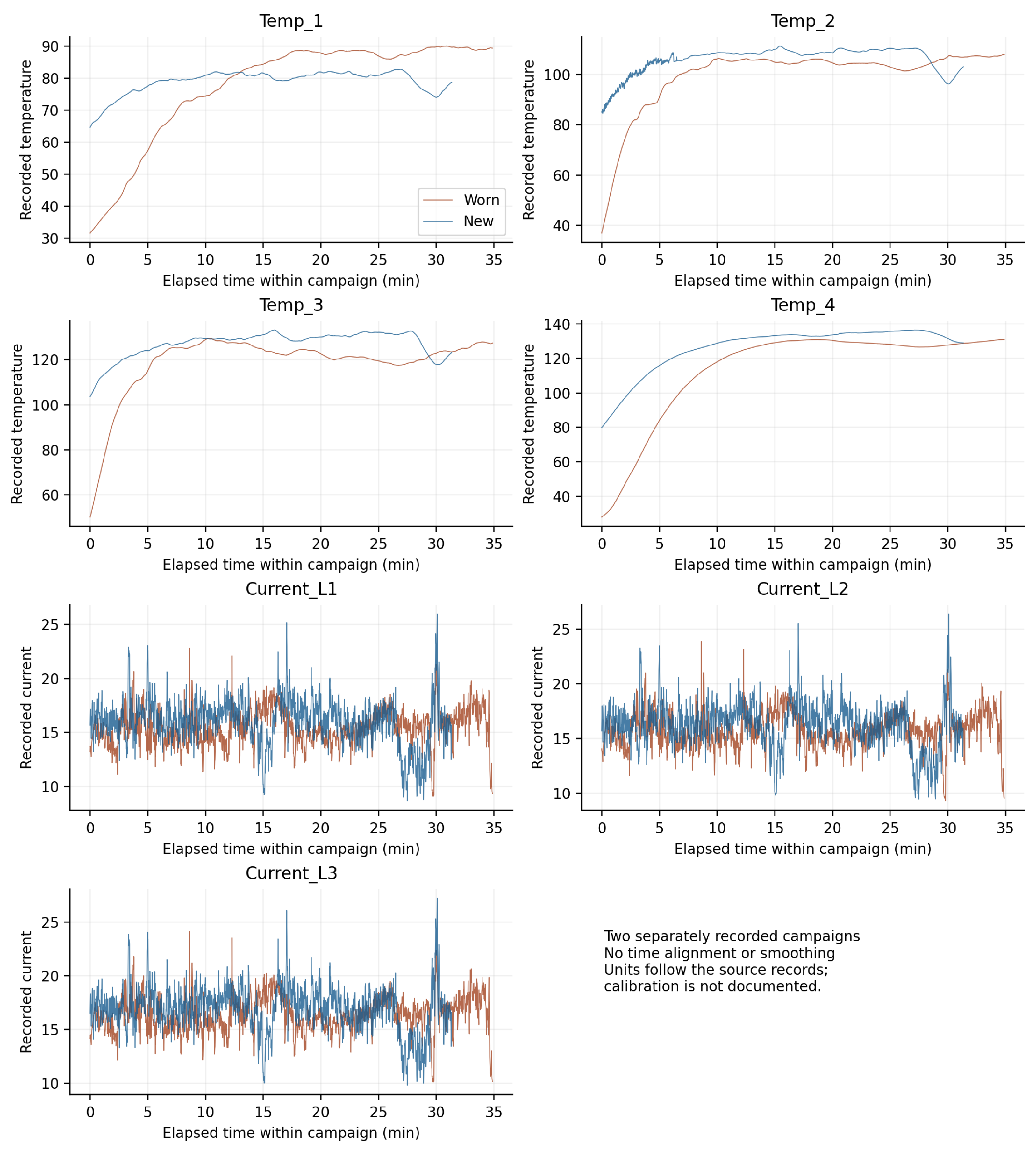
Table 6 provides descriptive results for all seven channels, and Figure 4 shows their complete recorded trajectories. Worn-record temperature means range from 77.71 to 118.97, compared with 78.94 to 127.12 in the new record; individual channel comparisons are given in the table. The trajectories contain substantial temperature increases, especially in the worn block. Temperature standard deviations are larger in that block for every channel. Current means are approximately 0.47–0.52 recorded units higher in the new block, while current standard deviations are also higher. These differences characterize the recorded campaigns and are not attributed specifically to wear.

Table 6. Descriptive signal statistics on the original recorded scale. Values are mean ± sample SD and median [first quartile, third quartile]. No unit calibration is inferred.

Channel	Worn Mean ± SD	New Mean ± SD	Worn Median [Q1,Q3]	New Median [Q1,Q3]
Temp_1	77.71 ± 16.03	78.94 ± 3.59	86.20 [72.86, 88.49]	80.37 [77.84, 81.34]
Temp_2	99.93 ± 12.60	106.11 ± 5.25	104.53 [101.81, 105.92]	108.17 [105.21, 109.48]
Temp_3	118.97 ± 13.41	127.12 ± 5.69	122.69 [119.52, 125.30]	129.24 [125.17, 130.81]
Temp_4	114.01 ± 27.25	126.62 ± 13.09	127.53 [112.56, 129.38]	132.68 [124.72, 134.78]
Current_L1	15.47 ± 1.62	15.98 ± 2.16	15.46 [14.46, 16.45]	16.15 [14.94, 17.14]
Current_L2	15.78 ± 1.59	16.25 ± 2.10	15.74 [14.88, 16.71]	16.37 [15.15, 17.38]
Current_L3	16.41 ± 1.63	16.92 ± 2.14	16.40 [15.44, 17.38]	17.07 [15.87, 18.08]

Figure 4. Complete temperature and current records against elapsed time within each campaign. Curves are raw retained values with no smoothing or temporal alignment; differences include trends and unrecorded operating effects.

Adjacent-record correlations exceed 0.998 for temperatures and range approximately 0.836–0.863 for currents. Trends contribute to these correlations; the coefficients are descriptive. The archive therefore cannot justify an analysis that treats all time rows as independent condition replicates. Neither the observed differences nor their variability alters the predictor-design aliasing.

3.6. Source-Cell Arithmetic and Observational Equivalence

Table 7 reproduces every workbook reduction and percentage using its actual operands. For Section 1, 65.48 − 64.43 gives 1.05 mm and 65.48 − 56.19 gives 9.29 mm. The upper percentage instead uses (65.02 − 56.19)/65.02 and gives 13.58%; dividing 9.29 by 65.48 would give 14.19%. This is a demonstrable difference between formula conventions, not a conclusion about which physical measurements should be paired. Source formulas and cached values are supplied for independent checking.

Table 7. Independently recalculated worksheet differences and ratios. Source F = B − D, G = B − E, H = (B − D)/B and I = (C − E)/C; ring rows use F and H only. Percentages below are 100 times the ratios.

Section	Excel Row	F (mm)	G (mm)	H (%)	I (%)
1	6	1.050	9.290	1.60	13.58
5	10	1.070	—	1.67	—
2	7	0.130	7.540	0.20	13.21
6	11	1.250	—	1.93	—
3	8	0.660	0.870	1.02	1.20
7	12	0.910	—	1.40	—
4	9	0.080	6.030	0.12	9.44
8	13	0.762	—	1.18	—

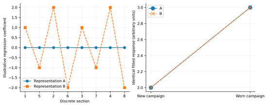
Figure 5 supplies a numerical illustration of Equation (9). Using the two diameter rows specified in Section 2.2 divided by 65 mm, representation A sets all eight coefficients to zero and the new/worn campaign coefficients to 2 and 3. Representation B adds the illustrative shift (1, −1, 2, −2, 1, −1, 2, −2) to the section coefficients and changes the campaign coefficients to 1.98406154 and 2.92446154. Both yield exactly the same fitted response, 2 in the new block and 3 in the worn block. Values are arbitrary response units and coefficient choices, not measured or reconstructed wear profiles. Floating-point checks are included in the supplement; exact equality follows algebraically from Equation (9).

Figure 5. Explicitly illustrative regression representations with identical fitted responses after compensating campaign effects. Coefficients are not physical section wear estimates.

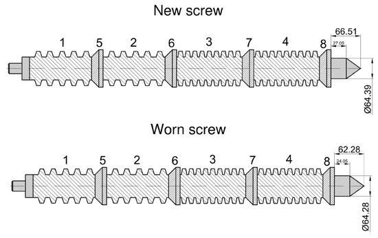
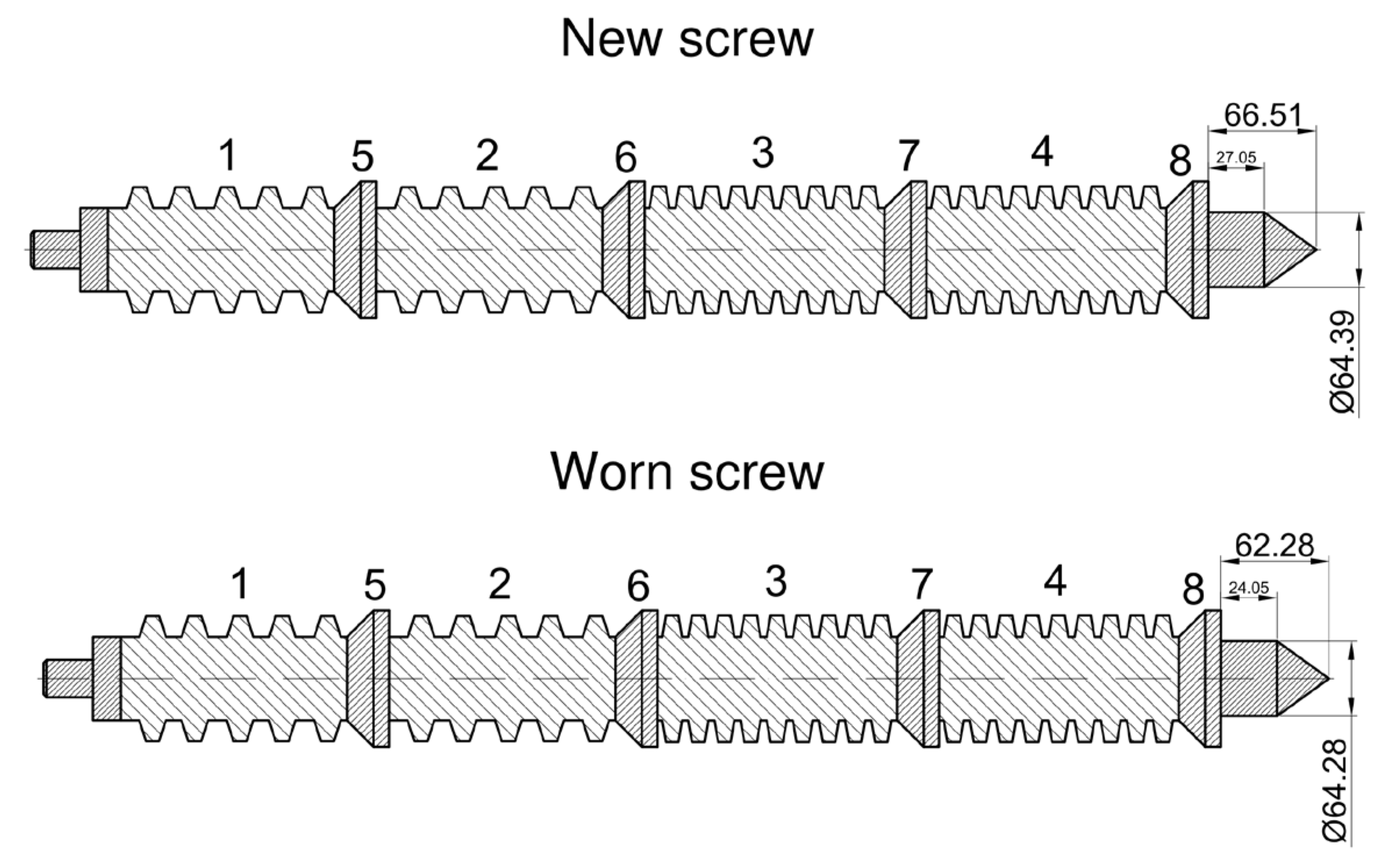
Figure 6 reproduces the available engineering drawing. Its labels establish discrete section order but do not document diameter measurement directions or paired datums.

Figure 6. Author-supplied drawing of new (upper) and worn (lower) screws. Labels have been translated into English. Section labels establish discrete order; diameter measurement surfaces, angular directions and paired datums are not documented.

4. Discussion

4.1. A Signal Contrast Is Not a Spatial Wear Estimate

The principal result is a precise boundary on inference. Under the campaign-adjusted model, the entire eight-column profile design is absorbed by the two campaign indicators. The data can contain visibly different temperatures or phase currents and still provide no campaign-adjusted information that separates one section from another. Under an intercept-only model, the records retain one between-campaign contrast, but that contrast is a property of two sequential blocks and cannot be uniquely attributed to a local wear component.

This distinction complements, rather than contradicts, signal-based extruder diagnostics. Earlier studies demonstrated that pressure, torque, current, and multi-source features can respond to wear or degradation [4,5,6,7]. The present result does not re-evaluate their classifiers or signal-separation metrics. It asks whether these specific observations identify a spatial parameter. A positive answer to a detection question does not imply a positive answer to a geometric inverse problem.

The relevant identifiability concept is model- and design-specific [13,14,15,16,17,18]. Here the failure is exact aliasing in the stated fixed-effect design, not merely a large standard error from poor numerical conditioning. The Frisch–Waugh–Lovell projection makes the distinction operational: once campaign effects are removed, no profile column remains. The same conclusion holds for any positive-definite weighting of the records because exact containment is preserved.

4.2. Why More Time Rows and Channels Do Not Resolve the Aliasing

The workbook contains nearly four thousand labeled rows, but the independent condition structure remains two contiguous campaigns with one record block per condition. Repeating rows with the same campaign membership scales the amount of data along the existing design pattern; it does not add a new direction to the profile design. Likewise, the seven response channels share the same campaign and profile columns. The multichannel extension increases the number of channel-specific coefficients, but it repeats the same rank defect for each channel.

This is not simply a shortage of time samples: it is exact confounding in the specified assignment and linear nuisance model. Additional independent geometry patterns are required, together with restrictions or measurements that prevent unrestricted campaign offsets from absorbing every geometry effect. Merely adding more campaigns, each with its own unrestricted fixed effect and campaign-constant geometry, would preserve the same aliasing. A future experiment must therefore change the observation-to-parameter structure, not only its sample count.

4.3. The Geometry Audit Is a Second, Independent Boundary

The dimensional audit exposes a separate limitation: reproducible arithmetic does not establish metrological comparability. Flight readings, ring diameters and endpoint labels are different record types. Table 5 and Table 7 make both the recorded values and their formula transformations explicit. Missing pairing information prevents selecting a physically preferred endpoint subtraction. Different percentage numerators and reversed labels are verified documentary features; their origin in measurement, transcription or worksheet construction cannot be inferred.

The established order 1–5–2–6–3–7–4–8 is still useful: it preserves the discrete axial sequence and makes the location labels auditable. It does not supply coordinates in millimetres or justify treating all eight values as comparable radial-loss measurements. Metrological practice requires an explicitly defined measurand, a traceable measurement procedure, and uncertainty information before a numerical estimate is treated as a calibrated engineering quantity [23,24]. The geometry audit therefore limits the target independently of the signal-design rank.

4.4. Contribution to Mechanical Engineering and Condition-Based Maintenance

For mechanical engineering, the practical contribution is an audit before a local inverse model or maintenance claim is accepted. The available signals can document a change between recorded operating histories; they cannot isolate wear from campaign conditions or prescribe a section-specific repair. Table 8 translates this boundary into decisions and additional evidence requirements.

Table 8. Maintenance inference supported by the present archive and evidence required for stronger claims.

Engineering Question	Present Evidence	Required Next Evidence
Do recorded operating histories differ?	Descriptive channel statistics and trajectories document differences.	Replicated controlled runs for repeatable condition effects.
Did screw wear cause the difference?	Not resolved: condition and campaign are confounded.	Operating inputs, batch logs, independent screws and crossed or interleaved tests.
Which section requires intervention?	No identifiable section coefficient after campaign adjustment.	Spatial sensitivity or local observations and a separately validated physical model.
How much material was lost?	Only source-defined diameter differences are reproducible.	Matched datums, defined measurand, repeatability and measurement uncertainty.
Can remaining life be predicted?	No validated degradation trajectory or failure threshold.	Longitudinal independent validation and a calibrated maintenance criterion.

The audit sequence provides a reusable check for similar inverse problems in rotating machinery, processing equipment, and condition-based maintenance: reconstruct the design, state the nuisance structure, project the parameters of interest, inspect the null space, and verify the geometry and measurand. This is a disciplined application of established rank and metrology principles [9,10,11,12,19,20,21,22,23,24], not a replacement for physical wear modelling or direct inspection. Its value is to prevent a signal-level difference from being reported as spatially resolved mechanical damage when the design and dimensional records do not support that inference.

4.5. Evidence Required for an Identifiable Axial Profile

A future study should pair process records with traceable before/after metrology on multiple independently measured screws. The physical sections should have fixed axial datums and documented millimetre coordinates; flight and ring geometries should be measured using a common stated measurand or reported as separate target types. Measurement repeatability, calibration, tolerance, and uncertainty should be retained. Process logs should include screw speed, feed, moisture, pressure, torque or calibrated shaft power, temperature, and throughput.

A prospective design should include multiple independently measured screw geometries tested at common operating settings, with screw state crossed with batches and measurement sessions where feasible. Within each session, interleave or randomize screw/configuration tests to avoid a state/order surrogate. Record speed, feed, moisture and loading synchronously, and repeat runs independently. Session nuisance terms must be shared across more than one geometry pattern, or constrained using independent measurements; one unrestricted intercept per constant-geometry run would again absorb its entire geometry contribution. For a campaign-level eight-predictor regression with only a global intercept, at least nine independently assigned profile rows are algebraically necessary for rank nine, but not sufficient: their centered patterns must span eight directions. More nuisance terms require a corresponding increase in independent design dimension. These are requirements for the prospective linear representation, not a guarantee of a physical wear reconstruction.

Before collection, evaluate the proposed residualized design under Equation (24), scaling heterogeneous predictors by declared reference values. Inspect the smallest nonzero singular value and its sensitivity to plausible measurement noise; select replication and target precision using an explicit noise model. Full column rank guarantees uniqueness of linear coefficients conditional on the model, but not accuracy, physical validity or useful uncertainty. A forward model with independent spatial sensitivities requires its own identifiability and validation analysis [13,14,15,16,17,18,25].

4.6. Limitations

This is a retrospective design and geometry audit of two condition blocks from one archive. The paper does not validate an operational classifier, establish a causal wear effect, estimate a nonlinear process model, or generalize a wear calibration to other screws or extruders. The campaign-adjusted zero rank is exact for the stated design representation; it does not prove that every possible nonlinear model of extrusion would be unidentifiable. Conversely, no nonlinear Fisher information is claimed because the required process model, synchronized inputs, and sensitivities are absent. The conclusions are limited to the evidence and geometry documentation inspected here.

5. Conclusions

• The campaign-constant geometry assignment adds no identifiable section-associated regression direction after unrestricted campaign adjustment. This exact result concerns the specified linear model and explains why temporal sampling density cannot substitute for independent spatial information.
• With an intercept-only nuisance specification, the design retains at most one between-campaign contrast, with seven profile directions unresolved. That contrast may describe a difference between the two recorded process blocks, but it cannot determine which screw section produced it or express wear in millimetres.
• Source-cell auditing makes the dimensional calculations reproducible while separating recorded diameter differences from verified material loss. The drawing establishes discrete axial order; absent pairing, datums and uncertainty prevent a calibrated eight-section wear target. Small documentary discrepancies alone do not demonstrate measurement error.
• In mechanical engineering practice, RAPID supports review of the evidence needed before process signals are converted into local maintenance decisions. Its output is a model-specific estimability statement and a traceable measurement audit. Future studies must decouple geometry from nuisance blocks, document operating inputs and local metrology, and assess precision and physical validity in addition to rank. These findings do not exclude thermal or electrical wear diagnosis in better documented designs.

References

- Klein, I. Predicting the Effect of Screw Wear on the Performance of Plasticating Extruders. Polym. Eng. Sci. 1975, 15, 444–450. [Google Scholar] [CrossRef] [Scilit]
- Yang, W.; Meng, W.; Gao, L.; Tan, Y.; Fottner, J.; Dai, X.; Yao, F.; Yuan, Y.; Sun, X. Analysis of the Screw Flight Wear Model and Wear Regularity of the Bulk Transport in Screw Ship Unloader. Iran. J. Sci. Technol. Trans. Mech. Eng. 2022, 46, 15–29. [Google Scholar] [CrossRef] [Scilit]
- Demirci, A.; Teke, I.; Polychronopoulos, N.D.; Vlachopoulos, J. The Role of Calender Gap in Barrel and Screw Wear in Counterrotating Twin Screw Extruders. Polymers 2021, 13, 990. [Google Scholar] [CrossRef] [Scilit] [PubMed]
- Ekielski, A.; Żelaziński, T.; Durczak, K. The Use of Wavelet Analysis to Assess the Degree of Wear of Working Elements of Food Extruders. Eksploat. Niezawodn. Maint. Reliab. 2017, 19, 560–564. [Google Scholar] [CrossRef] [Scilit]
- Danielak, M.; Witaszek, K.; Ekielski, A.; Żelaziński, T.; Dudnyk, A.; Durczak, K. Wear Detection of Extruder Elements Based on Current Signature by Means of a Continuous Wavelet Transform. Processes 2023, 11, 3240. [Google Scholar] [CrossRef] [Scilit]
- Park, J.K.; Lee, H.; Kim, W.; Kim, G.M.; An, D. Degradation Feature Extraction Method for Prognostics of an Extruder Screw Using Multi-Source Monitoring Data. Sensors 2023, 23, 637. [Google Scholar] [CrossRef] [Scilit] [PubMed]
- Durczak, K.; Witaszek, K.; Adamczyk, F.; Szaroleta, M. Non-Invasive Electrical Detection of Screw Wear in an Industrial Extrusion System. J. Res. Appl. Agric. Eng. 2026, 71, 58–64. [Google Scholar] [CrossRef] [Scilit]
- Taki, K.; Sugiyama, T.; Ohara, M.; Umemoto, S.; Tanifuji, S.; Murata, J.; Tsujimura, I.; Kihara, S. Online Monitoring of the Degree of Fill in a Rotating Full-Flight Screw of a Corotating Twin-Screw Extruder. AIChE J. 2019, 65, 326–333. [Google Scholar] [CrossRef] [Scilit]
- Jardine, A.K.S.; Lin, D.; Banjevic, D. A Review on Machinery Diagnostics and Prognostics Implementing Condition-Based Maintenance. Mech. Syst. Signal Process. 2006, 20, 1483–1510. [Google Scholar] [CrossRef] [Scilit]
- Lei, Y.; Li, N.; Guo, L.; Li, N.; Yan, T.; Lin, J. Machinery Health Prognostics: A Systematic Review from Data Acquisition to Remaining Useful Life Prediction. Mech. Syst. Signal Process. 2018, 104, 799–834. [Google Scholar] [CrossRef] [Scilit]
- Quatrini, E.; Costantino, F.; Di Gravio, G.; Patriarca, R. Condition-Based Maintenance—An Extensive Literature Review. Machines 2020, 8, 31. [Google Scholar] [CrossRef] [Scilit]
- Benbouzid, M.E.H. A Review of Induction Motors Signature Analysis as a Medium for Faults Detection. IEEE Trans. Ind. Electron. 2000, 47, 984–993. [Google Scholar] [CrossRef] [Scilit]
- Bellman, R.; Åström, K.J. On Structural Identifiability. Math. Biosci. 1970, 7, 329–339. [Google Scholar] [CrossRef] [Scilit]
- Rothenberg, T.J. Identification in Parametric Models. Econometrica 1971, 39, 577–591. [Google Scholar] [CrossRef] [Scilit]
- Richmond, J. Identifiability in Linear Models. Econometrica 1974, 42, 731–736. [Google Scholar] [CrossRef] [Scilit]
- Chis, O.-T.; Banga, J.R.; Balsa-Canto, E. Structural Identifiability of Systems Biology Models: A Critical Comparison of Methods. PLoS ONE 2011, 6, e27755. [Google Scholar] [CrossRef] [Scilit] [PubMed]
- Miao, H.; Xia, X.; Perelson, A.S.; Wu, H. On Identifiability of Nonlinear ODE Models and Applications in Viral Dynamics. SIAM Rev. 2011, 53, 3–39. [Google Scholar] [CrossRef] [Scilit] [PubMed]
- Castro, M.; de Boer, R.J. Testing Structural Identifiability by a Simple Scaling Method. PLoS Comput. Biol. 2020, 16, e1008248. [Google Scholar] [CrossRef] [Scilit] [PubMed]
- Frisch, R.; Waugh, F.V. Partial Time Regressions as Compared with Individual Trends. Econometrica 1933, 1, 387–401. [Google Scholar] [CrossRef] [Scilit]
- Lovell, M.C. Seasonal Adjustment of Economic Time Series and Multiple Regression Analysis. J. Am. Stat. Assoc. 1963, 58, 993–1010. [Google Scholar] [CrossRef]
- Hurlbert, S.H. Pseudoreplication and the Design of Ecological Field Experiments. Ecol. Monogr. 1984, 54, 187–211. [Google Scholar] [CrossRef] [Scilit]
- Lazic, S.E. The Problem of Pseudoreplication in Neuroscientific Studies: Is It Affecting Your Analysis? BMC Neurosci. 2010, 11, 5. [Google Scholar] [CrossRef] [Scilit] [PubMed]
- Joint Committee for Guides in Metrology. Evaluation of Measurement Data—Guide to the Expression of Uncertainty in Measurement (JCGM 100:2008); BIPM: Sèvres, France, 2008. [Google Scholar] [CrossRef] [Scilit]
- Joint Committee for Guides in Metrology. International Vocabulary of Metrology—Basic and General Concepts and Associated Terms (VIM), 3rd ed.; JCGM 200:2012; BIPM: Sèvres, France, 2012. [Google Scholar] [CrossRef] [Scilit]
- Atkinson, A.C.; Donev, A.N. Optimum Experimental Designs; Oxford Statistical Science Series; Oxford University Press: Oxford, UK, 1992. [Google Scholar]
Disclaimer/Publisher’s Note: The statements, opinions and data contained in all publications are solely those of the individual author(s) and contributor(s) and not of MDPI and/or the editor(s). MDPI and/or the editor(s) disclaim responsibility for any injury to people or property resulting from any ideas, methods, instructions or products referred to in the content. |
© 2026 by the authors. Licensee MDPI, Basel, Switzerland. This article is an open access article distributed under the terms and conditions of the Creative Commons Attribution (CC BY) license.