A Positive-Only Conditional Normalizing Flow to Assess Lightning-Caused Fires According to Meteorological Condition

Abstract

Lightning-caused fires (LCFs) are an important forest disturbance closely associated with meteorological conditions. However, reliable non-fire samples are difficult to define because the absence of recorded fires does not necessarily indicate unsuitable fire conditions, limiting conventional binary classification. The purpose of this study is to develop a positive-only framework for assessing the meteorological compatibility of LCFs using verified historical fire records. Using 984 verified LCF records from the Daxing’anling forest region, China, a Positive-Only Spatiotemporal Conditional Normalizing Flow with Context-Mismatch Learning (PO-STCNF-CM) was developed to characterize LCF-associated meteorological conditions across spatial and seasonal contexts. The model incorporates same-day event weighting and context-mismatch learning, and a Meteorological Compatibility Index (MCI) converts density-based anomaly scores into an interpretable 0–100 scale. GMM provided strong likelihood fitting, while ablation analysis showed that spatiotemporal conditioning improved neural density fitting and context-mismatch learning strengthened contextual discrimination. For the held-out records, PO-STCNF-CM produced a mean MCI of 53.761, a median MCI of 57.169, and an 80% coverage error of 0.015. The proposed framework provides an interpretable approach for characterizing LCF-associated meteorological conditions without requiring artificial non-fire samples.

1. Introduction

Lightning-caused fires (LCFs) are an important source of natural ignition in forest and grassland ecosystems, with lightning being the predominant natural cause of wildfires [1,2]. Their occurrence is strongly influenced by conditions surrounding ignition, particularly fuel moisture, precipitation, temperature, and other fire-weather factors. Precipitation around lightning events can determine whether an ignition persists and develops into a detectable fire, while regional environmental differences can further influence lightning-fire occurrence [3,4]. Compared with human-caused fires, LCFs occur more frequently in remote areas and under dry fuel conditions, making timely detection and suppression more difficult [5]. In extratropical forests, lightning accounts for a substantial proportion of fire activity and burned area, with important consequences for forest loss and carbon emissions. Climate warming may further increase lightning activity and fuel dryness in these regions, potentially increasing the contribution of lightning fires to future fire activity. Therefore, characterizing the meteorological conditions associated with historical LCF events is important for understanding LCF-associated weather patterns and supporting meteorologically informed forest-fire management [6,7].

With advances in meteorological observations, remote sensing, and artificial intelligence, substantial progress has been made in forest fire danger assessment and LCF modelling. Traditional approaches commonly use fire-weather indices, empirical thresholds, statistical regression, or spatial analysis to characterize fire-prone conditions based on meteorological, topographic, and vegetation variables. These methods are generally interpretable and have been widely applied to regional fire-danger assessment and management [6,8]. More recently, machine learning and deep learning methods, including random forests, support vector machines, gradient boosting, and neural networks, have been increasingly used to capture nonlinear relationships among multiple environmental factors in wildfire susceptibility mapping, fire occurrence prediction, fire detection, and lightning-fire modelling [8,9,10].

Forest fire danger assessment has developed through several methodological pathways, including empirical, deterministic, statistical, probabilistic, hybrid, and simulation-based approaches [11,12]. Empirical methods commonly use weather- or fuel-based indices, experimentally derived relationships, and threshold-based formulations to summarize fire-prone environmental conditions, whereas deterministic approaches represent fire behaviour and spread using physical or process-based relationships involving fuel properties, weather, combustion, heat transfer, and terrain. Statistical and probabilistic methods, including regression, count models, spatial models, and stochastic approaches, estimate fire occurrence or behaviour from historical observations and provide a means of representing variability and uncertainty. Deterministic and probabilistic components can also be combined in integrated frameworks, while simulation models are widely used to reproduce fire growth and spread under different environmental conditions. More recently, machine learning and deep learning have extended these approaches by learning nonlinear relationships from multi-source meteorological, remote-sensing, vegetation, and spatial data [13]. Operational fire-danger rating systems provide well-established examples of these approaches. In Canada, the Canadian Forest Fire Danger Rating System (CFFDRS), particularly its Canadian Forest Fire Weather Index (FWI) System, converts weather observations into fuel-moisture codes and fire-behaviour indices that support operational fire-danger assessment [14]. In the United States, the National Fire Danger Rating System (NFDRS) integrates weather, fuel, and fire-occurrence information to provide operational measures of fire danger, and its recent version 4 incorporates updated live- and dead-fuel moisture models and simplified fuel classifications [15]. Although these systems are not designed exclusively for lightning-caused fires, their meteorological and fuel-moisture components are highly relevant to lightning-fire assessment. Recent studies have further shown that lightning-caused fire occurrence depends on the combined effects of lightning characteristics, precipitation, fuel moisture, vegetation, and other environmental conditions [4]. Such findings demonstrate that operational fire-danger systems and lightning-specific models provide complementary perspectives for assessing the environmental conditions associated with lightning-caused fires.

Machine learning has also shown potential for lightning-fire prediction. Existing studies have used lightning forecasts and environmental conditions to predict fire ignition, while recent work in northeast China has combined igniting and non-igniting lightning cases with meteorological, soil, topographic, vegetation, and lightning variables [3,16,17]. However, LCF occurrence depends on interacting factors such as lightning activity, fuel conditions, precipitation, drought, and local environmental variability. Their relationships can also vary across locations and seasons, making fixed meteorological thresholds difficult to apply consistently across different environmental settings [3,4]. Importantly, many wildfire and lightning-fire prediction models are formulated as binary classification problems and therefore require both fire and non-fire observations or, in lightning-ignition studies, igniting and non-igniting lightning samples [18]. Reliable non-fire samples are not always available in historical LCF datasets. The absence of a recorded fire does not necessarily represent unsuitable fire conditions, particularly when complete information on lightning exposure, fuel conditions, and non-igniting lightning is unavailable. Treating such observations as negative samples may therefore introduce uncertainty into model training and interpretation. This limitation motivates a different approach that learns directly from observed LCF events without requiring explicitly defined non-fire samples.

The difficulty of defining reliable non-fire samples is particularly important for LCF modelling because ignition depends on the combined effects of lightning activity, fuel conditions, precipitation, drought, and local environmental variability [19]. Recent studies have shown that fuel characteristics, moisture conditions, fire-weather variables, and geographical factors jointly influence whether lightning strikes develop into wildfires [20,21]. These interacting factors can produce nonlinear relationships that vary across environmental settings, which has motivated the increasing use of machine learning for fire-danger and ignition-related modelling [22]. However, when complete lightning exposure and non-ignition records are unavailable, locations or times without recorded fires cannot be confidently regarded as true negative observations. A location may experience meteorological conditions favourable for LCF but remain unlabelled because lightning ignition did not occur or the event was not detected [23]. Consequently, treating unobserved locations as negative samples may introduce pseudo-absence bias and affect both model training and interpretation [24]. This problem creates a need for modelling approaches that can characterize LCF-associated environmental conditions using observed fire records without relying on uncertain negative samples.

To address the absence or unreliability of non-fire samples, positive-only learning and presence-only modelling provide an alternative framework for studying environmental conditions associated with observed events. Unlike conventional binary classification, these approaches do not require a boundary to be learned between fire and non-fire conditions. Instead, they characterize the range and distribution of environmental conditions represented by observed target events and can be used to determine how typical a new observation is relative to those conditions [25,26]. Such approaches have been applied in ecological distribution modelling, anomaly detection, and one-class classification when only presence records or target-class samples are available [27,28,29,30]. For LCF studies, when reliable non-fire records, non-igniting lightning samples, or complete background observations are unavailable, estimating an absolute probability of fire occurrence is not an appropriate objective [29,30]. Instead, the meteorological conditions associated with historical LCF events can be characterized, and new conditions can be evaluated according to how closely they resemble these historical conditions. Existing positive-only and one-class approaches, however, have mainly focused on classification, anomaly detection, or environmental suitability assessment, with less attention to how event-associated meteorological patterns vary with location and season [31]. Therefore, this study develops a positive-only framework that models the meteorological conditions associated with historical LCF events in their spatial and seasonal contexts. Context-mismatch learning is further introduced to help the model distinguish whether observed meteorological conditions are consistent with their corresponding location and season.

To model LCF-associated meteorological conditions using only positive records, this study proposes a Positive-Only Spatiotemporal Conditional Normalizing Flow with Context-Mismatch Learning (PO-STCNF-CM), developed using 984 historical LCF records from the Daxing’anling forest region, China. The model characterizes the distribution of meteorological conditions associated with recorded LCF events while accounting for differences in location and season. Specifically, a conditional normalizing flow is used to learn how LCF-associated meteorological patterns vary across spatial and seasonal contexts. Same-day event weighting reduces the influence of dates with clustered fire records, while context-mismatch learning encourages the model to assign greater compatibility to meteorological conditions under their observed contexts than under unrelated contexts. Model-derived anomaly scores are then converted into a 0–100 Meteorological Compatibility Index (MCI) through percentile-based calibration against historical LCF records. Unlike conventional binary fire prediction, the proposed framework does not require artificially constructed non-fire samples or estimate absolute fire occurrence probabilities. Instead, it quantifies how closely a meteorological condition resembles those associated with historical LCF events under comparable spatial and seasonal contexts. The purpose of this study is to develop an interpretable positive-only framework for assessing the meteorological compatibility of lightning-caused fires when reliable negative samples are unavailable. Accordingly, the specific objectives are to: (1) develop a spatiotemporal conditional density model for characterizing meteorological conditions associated with historical LCF events; (2) construct an interpretable MCI for quantifying the relative meteorological compatibility of LCF-associated conditions under different spatial and seasonal contexts; and (3) evaluate the proposed framework using chronological held-out records in terms of density fitting, calibration consistency, and meteorological–context association.

2. Materials and Methods

2.1. Study Area and Dataset

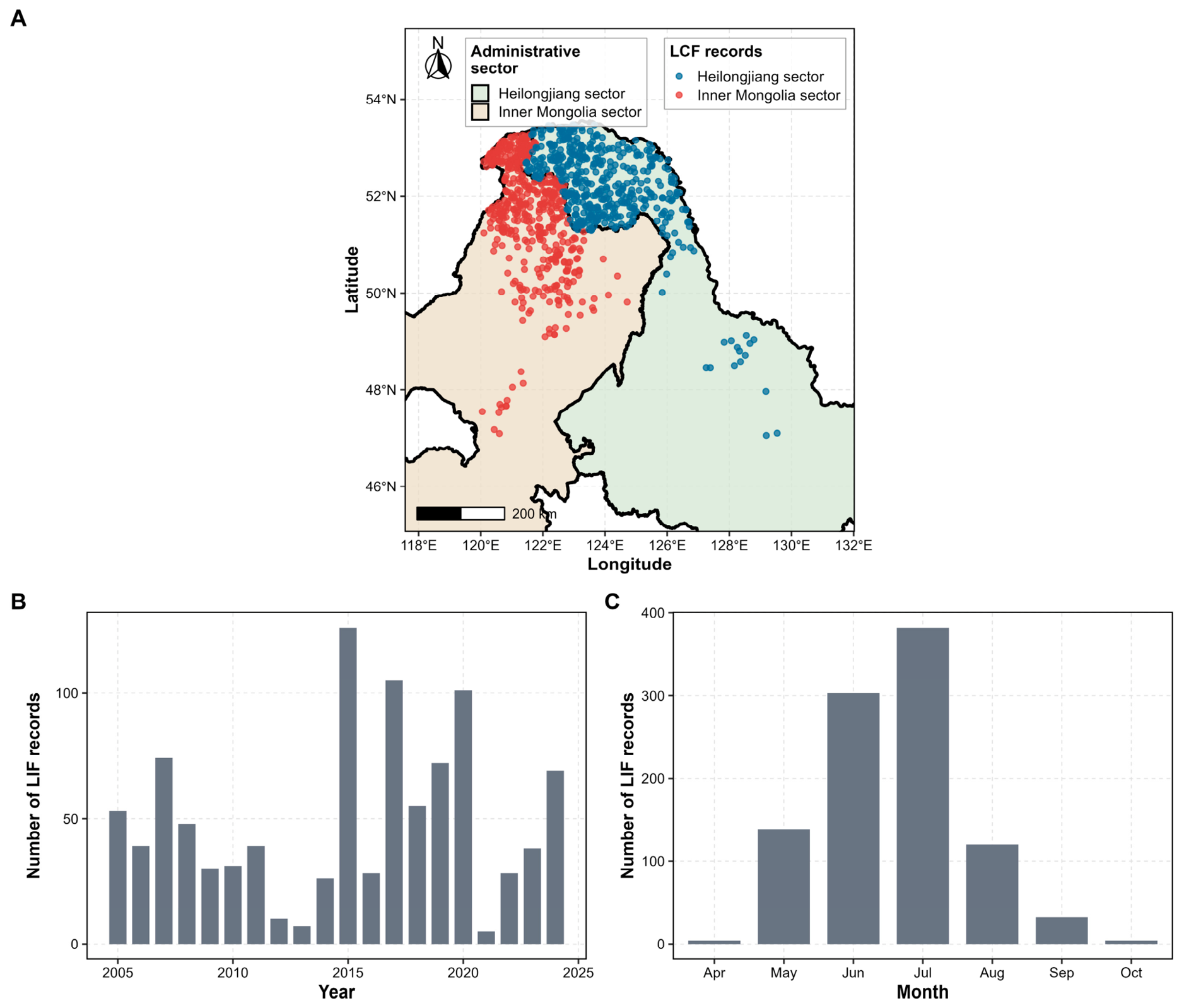
The study area is located in the Daxing’anling forest region of northeastern China, extending across parts of Inner Mongolia and Heilongjiang. The region contains extensive forest ecosystems and is characterized by pronounced seasonal variations in temperature and precipitation, with lightning-caused fires occurring mainly during the warm season. These spatial and seasonal characteristics make the region suitable for examining the meteorological conditions associated with historical LCF events. The dataset used in this study comprises historical LCF records and corresponding meteorological observations from the Daxing’anling forest region, China. The meteorological data were provided by the CMA Public Meteorological Service Centre. The 11 meteorological variables used for LCF compatibility modelling, together with their definitions and units, are summarized in Table 1. After manual verification and data cleaning, 984 LCF records with valid occurrence dates and geographical coordinates were retained, covering the period from 23 May 2005 to 20 August 2024. The study region spans parts of Inner Mongolia and Heilongjiang; therefore, each record was assigned an administrative-sector label according to its geographical location. Of the 984 records, 514 were located in the Inner Mongolia sector and 470 in the Heilongjiang sector. The administrative-sector label was included as regional contextual information in the subsequent modelling rather than being used to define separate province-based samples. The spatial and temporal coverage of the dataset is summarized in Figure 1.

Table 1. Meteorological variables used for LCF compatibility modelling.

Meteorological Variable	Description	Unit	Meteorological Variable	Description	Unit
Mean temperature	Daily mean air temperature	°C	30-day mean temperature	Mean temperature over the preceding 30-day period	°C
Maximum temperature	Daily maximum air temperature	°C	Previous 24 h precipitation	Precipitation accumulated over the previous 24 h	mm
Minimum temperature	Daily minimum air temperature	°C	Previous 3-day precipitation	Precipitation accumulated over the previous 3 days	mm
Daily precipitation	Precipitation recorded for the event day	mm	Previous 10-day precipitation	Precipitation accumulated over the previous 10 days	mm
10-day mean temperature	Mean temperature over the preceding 10-day period	°C	Previous 30-day precipitation	Precipitation accumulated over the previous 30 days	mm
Drought index	Index characterizing antecedent drought conditions	-	-

Figure 1. Overview of the historical lightning-caused fire dataset in the Daxing’anling forest region. (A) Spatial distribution of valid LCF records with administrative-sector background. Administrative boundaries indicate the Inner Mongolia and Heilongjiang sectors and do not represent independent sampling regions. (B) Annual distribution of LCF records. (C) Monthly distribution of LCF records.

Each record corresponds to an observed LCF event and contains the occurrence date, geographical location, administrative-sector label, ignition unit or site, and meteorological conditions during and before the event. Eleven meteorological variables were used to characterize three aspects of the weather conditions associated with LCF events: temperature, precipitation, and drought. The temperature variables comprised mean, maximum, and minimum temperature, together with 10-day and 30-day mean temperature. The precipitation variables comprised daily precipitation and accumulated precipitation over the previous 24 h, 3 days, 10 days, and 30 days. A drought index was included to characterize the regional drought background. The day of the year was derived from the occurrence date to represent seasonal variation, while longitude, latitude, and the administrative-sector label were used to provide spatial and regional context for subsequent modelling.

Because the dataset contains only recorded LCF events and lacks reliable non-fire samples or non-igniting lightning records, it was treated as a positive-only LCF meteorological dataset [24,26,28]. Accordingly, the analysis focuses on characterizing meteorological conditions associated with historical LCF events rather than estimating an absolute probability of fire occurrence. Temperature-related variables were standardized, whereas precipitation-related variables were transformed using log1p to reduce skewness while retaining zero-precipitation observations. Same-day event weighting was applied during model training, and date-clustered bootstrap resampling was used during evaluation to reduce the influence of multiple LCF records occurring on the same date.

2.2. Positive-Only Spatiotemporal Compatibility Modelling Framework

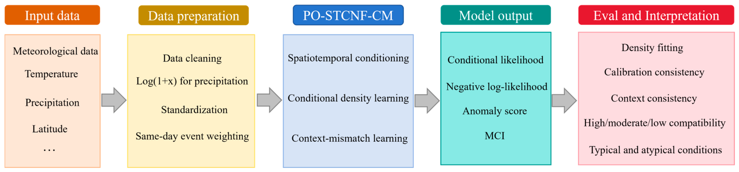
The proposed framework consists of three main components. First, the LCF assessment problem is formulated using only observed fire records, without requiring artificially constructed non-fire samples. Second, a Positive-Only Spatiotemporal Conditional Normalizing Flow with Context-Mismatch Learning (PO-STCNF-CM) is used to characterize how LCF-associated meteorological conditions vary with location and season. Same-day event weighting is incorporated to reduce the influence of temporally clustered records, while context-mismatch learning encourages the model to distinguish observed meteorological–context combinations from mismatched ones. Third, the model-derived anomaly score is converted into a Meteorological Compatibility Index (MCI), providing an interpretable measure of how closely a meteorological condition resembles those associated with historical LCF events under comparable spatial and seasonal contexts. MCI represents meteorological compatibility rather than the absolute probability of fire occurrence. The overall workflow of the proposed framework is illustrated in Figure 2.

Figure 2. Workflow of the proposed positive-only framework for meteorological compatibility assessment of lightning-caused fires. Historical LCF records and meteorological–contextual data were processed and chronologically partitioned into training, calibration, and held-out evaluation subsets. PO-STCNF-CM was then used for conditional density modelling and context-mismatch learning, followed by percentile-based MCI calibration and held-out compatibility assessment.

2.2.1. Positive-Only Conditional Density Formulation

Because the dataset consisted only of observed lightning-caused fire (LCF) records, reliable non-fire samples were not available for conventional supervised classification. The absence of a recorded LCF event was not considered evidence of unsuitable fire conditions, because locations or dates without recorded fires may still have experienced favourable meteorological conditions but lacked lightning ignition, suitable fuel conditions, or reliable fire detection [24,32]. Therefore, LCF assessment was formulated as a positive-only meteorological compatibility problem rather than a binary fire/non-fire prediction task [33,34,35].

In this formulation, the model learns the meteorological conditions represented by historical LCF events and how these conditions vary across different locations and seasons. For each observed LCF record, the meteorological vector was denoted by x_i and contained the temperature-, precipitation-, and drought-related variables described in Section 2.1. The corresponding context vector, c_i, contained longitude, latitude, day of year, and the administrative-sector label. Rather than learning a single meteorological distribution for the entire study region, the model estimates the conditional density p_θ(x_i|c_i), which describes how well a meteorological state x_i is represented by historical LCF-associated conditions under context c_i.

The resulting density was not interpreted as the probability of fire occurrence. Instead, it provided the basis for evaluating the meteorological compatibility of a given condition with historical LCF events under a specified spatial and seasonal context. Higher compatibility indicates that the condition more closely resembles meteorological states represented in the historical LCF records, whereas lower compatibility indicates that it is less typical of those records.

2.2.2. Context-Mismatch Enhanced Spatiotemporal Normalizing Flow

To model the potentially complex distribution of LCF-associated meteorological conditions, this study used a spatiotemporal conditional normalizing flow. A normalizing flow is a probabilistic model that represents a complex data distribution by transforming the observed variables into a simpler reference distribution through a sequence of invertible transformations. Because these transformations are reversible, the density of an observed meteorological state can be evaluated directly. In this study, the transformations were conditioned on spatial and seasonal information, allowing the learned meteorological distribution to vary across different contexts [34,36]. Following the standard change-of-variables formulation for normalizing flows [36,37], the conditional log-likelihood of each observed LCF record was calculated as:

$$\log P_{\theta }(x_i|c_i)=\log P(z_i)+\log \left|\det \left({\displaystyle \frac{\partial f_{\theta }(x_i;c_i)}{\partial x_i}}\right)\right|$$

(1)

where z_i is the latent representation obtained by the context-conditioned invertible mapping f_θ, f_θ denotes the normalizing-flow transformation, and P(z_i) is the base density. The model was trained by minimizing the negative log-likelihood of observed LCF records. To reduce the potential dominance of dates with multiple recorded events, same-day event weighting was applied in the NLL term. Each record was weighted by $w_i={\displaystyle \frac{1}{\sqrt{n_{d\left(i\right)}}}}$, where n_d(i) denotes the number of records occurring on the same ignition date as record i.

In addition to fitting the observed meteorological conditions, the model was designed to learn whether these conditions were associated with the appropriate spatial and seasonal context. For this purpose, context-mismatch learning was introduced [38]. For each observed meteorological–context pair (x_i, c_i), a mismatched context $c_i^{-}$ was generated by pairing the same meteorological vector with an incorrect contextual vector sampled from other records. The model was encouraged to assign a higher likelihood to the observed pair than to the mismatched pair. The context-mismatch loss was defined as:

$$L_{\mathit{cm}}={\displaystyle \frac{1}{N}}{\displaystyle {\sum }_{i=1}^N\max \left[0,m-\log p_{\theta }(x_i|c_i)+\log P_{\theta }(x_i|c_i^{-})\right]}$$

(2)

where m is the margin parameter specifying the desired likelihood separation between the observed and mismatched meteorological–context pairs. This loss does not introduce artificial non-fire samples. Instead, it acts as a context-level contrastive constraint that encourages the model to learn whether a meteorological condition is compatible with its spatial and seasonal background.

The resulting model was termed the Positive-Only Spatiotemporal Conditional Normalizing Flow with Context-Mismatch Learning (PO-STCNF-CM). Its overall training objective combined the weighted NLL, context-mismatch loss, and a regularization term:

L = L_NLL + λ_cmL_cm + λ_regL_reg

(3)

where L_NLL denotes the weighted negative log-likelihood loss used to fit the conditional density of the observed LCF records, L_cm denotes the context-mismatch loss, and L_reg denotes the regularization term. The coefficients λ_cm and λ_reg control the contributions of context-mismatch learning and regularization, respectively.

2.2.3. Meteorological Compatibility Index and Calibrated Interpretation

Although the conditional density provides a quantitative measure of how well a meteorological condition is represented under a given spatial and seasonal context, its numerical value is not directly intuitive for practical interpretation. Therefore, the model output was converted into a Meteorological Compatibility Index (MCI), a 0–100 scale that expresses the relative compatibility of a meteorological condition with historical LCF-associated conditions. MCI is derived from the model output through a calibration step and is not an additional component of the neural network. First, the anomaly score of record i was defined as the negative log-likelihood:

A_i = −log p_θ(x_i|c_i)

(4)

where x_i denotes the meteorological variable vector and c_i denotes the corresponding spatiotemporal contextual vector. A lower anomaly score indicates that the meteorological condition is more consistent with the historical LCF-associated meteorological distribution under the given spatial and seasonal context.

To make anomaly scores comparable and easier to interpret, each score was converted into a percentile relative to the historical calibration set using a rank-based procedure following the principle used in conformal methods [39,40]:

$${\mathrm{MCI}}_i=100\times T_i=100\times {\displaystyle \frac{1+{\displaystyle {\sum }_{j=1}^{n_{\mathit{cal}}}\mathbb{I}(A_j^{\mathit{cal}}\ge A_i)}}{n_{\mathit{cal}}+1}}$$

(5)

where $A_j^{\mathit{cal}}$ denotes the anomaly score of calibration record j, and n_cal is the number of records in the calibration set. MCI ranges from 0 to 100, with higher values indicating stronger compatibility with historical LCF-associated meteorological conditions. In other words, a high MCI indicates that the meteorological condition is highly typical of the historical positive-fire calibration distribution, whereas a low MCI indicates that the condition is less represented among historical LCF records.

MCI is a study-defined measure of meteorological compatibility and should not be interpreted as an absolute probability of LCF occurrence, a binary fire/non-fire prediction, or an official fire-danger class. It provides a relative and interpretable measure of how typical a meteorological condition is compared with historical LCF-associated conditions. For model comparison, outputs from all baseline models were converted to MCI using the same calibration procedure, allowing compatibility-related metrics to be evaluated on a common scale.

2.3. Experimental Design and Implementation Details

To evaluate PO-STCNF-CM under positive-only data conditions, the 984 historical LCF records were divided chronologically into training, calibration, and held-out evaluation subsets. A chronological split was used to reduce temporal information leakage [41]. Records from 2005–2018 were used for model training, records from 2019–2021 were used for MCI calibration, and records from 2022–2024 were completely withheld from both model training and calibration and used only for retrospective evaluation. This design allowed the model to learn from earlier historical records and evaluate the meteorological compatibility of later LCF events without using future records during model fitting or calibration.

The composition of the chronological subsets is summarized in Table 2. The analysis-ready dataset contained 984 LCF records representing 403 unique event dates, and no additional records were excluded during computational preprocessing. Of these, 671 records from 277 unique event dates were assigned to the training subset, 178 records from 54 unique event dates to the calibration subset, and 135 records from 72 unique event dates to the held-out evaluation subset. The held-out subset contained records from both administrative sectors (52 from Inner Mongolia and 83 from Heilongjiang) and was dominated by summer events, consistent with the seasonal distribution of the overall dataset. These records were not used during either model training or MCI calibration.

Table 2. Composition of the chronological training, calibration, and held-out evaluation subsets.

Dataset	Period	Records	Unique Event Dates	Inner Mongolia	Heilongjiang	Spring	Summer	Autumn	Winter
All	2005–2024	984	403	514	470	142	805	36	0
Training	2005–2018	671	277	331	340	109	528	34	0
Calibration	2019–2021	178	54	131	47	17	160	1	0
Held-out evaluation	2022–2024	135	72	52	83	17	117	1	0

Note: Seasons were defined as spring (March–May), summer (June–August), autumn (September–November), and winter (December–February).

All preprocessing parameters were estimated from the training subset and subsequently applied unchanged to the calibration and held-out subsets. Precipitation-related variables were transformed using log(1 + x) to reduce skewness while retaining zero-precipitation observations. Temperature-related variables, drought index, transformed precipitation variables, and spatial coordinates were then standardized. Seasonal variation was represented by sine and cosine transformations of the day of year, thereby avoiding the discontinuity between the end and beginning of a calendar year. The administrative-sector label was included as a categorical contextual variable.

The model received the 11 meteorological variables as the input vector and longitude, latitude, sine–cosine day-of-year encodings, and administrative-sector label as contextual information. The context vector was mapped to a contextual embedding using a multilayer perceptron and then used to condition the neural spline flow transformations. PO-STCNF-CM was trained using the weighted negative log-likelihood together with the context-mismatch loss described in Section 2.2. Same-day weighting was applied during training, and mismatched contexts were generated within each mini-batch by pairing meteorological vectors with contextual vectors from other records.

Model parameters were optimized using the AdamW optimizer, which decouples weight decay from the gradient-based parameter update and is commonly used for regularized training of deep neural networks [42]. The learning rate was set to 1 × 10⁻³, and the weight-decay coefficient was set to 1 × 10⁻⁵. AdamW updates were applied to all trainable model parameters. The main hyperparameters included the learning rate, batch size, number of flow layers, hidden dimension, context embedding dimension, context-mismatch margin, and context-mismatch loss weight. The context-mismatch margin was set to 0.5, and the corresponding loss weight was set to 0.20. All models were implemented in Python 3.12 using PyTorch 2.7 and PyTorch Lightning 2.5. The proposed methodology was implemented with custom-written Python code, and no commercial modelling software was used. Model training, calibration, and evaluation were performed within the same software environment on an NVIDIA GeForce RTX 5090 GPU with 32 GB of GPU memory. Across the three repeated runs, complete PO-STCNF-CM training, including epoch selection and final refitting, required 111.46 ± 55.29 s per run. After model training and calibration, MCI calculation for the 135 chronologically held-out records required 0.181 ± 0.028 s, corresponding to 1.34 ± 0.21 ms per event. The MCI runtime was measured over 100 repeated evaluations after GPU warm-up and included input preprocessing, model scoring, and MCI conversion.

To account for variability arising from random initialization and stochastic optimization, PO-STCNF-CM was trained repeatedly using multiple random seeds. The data split, feature construction, preprocessing, and evaluation procedures were kept identical across runs. Performance was summarized using the mean and standard deviation across repeated runs. For sample-level MCI distributions and case-based interpretation, a representative model was selected based on its likelihood performance on the calibration subset.

Model evaluation considered three aspects: density fitting, MCI calibration, and context consistency. The mean, median, and weighted mean negative log-likelihood (NLL) were used to evaluate density fitting. Mean and median MCI summarized the compatibility of held-out LCF records with historical LCF-associated meteorological conditions. The 80% coverage error measured the deviation between the observed and expected proportion of records within the corresponding calibration region, while the context likelihood margin quantified the likelihood difference between observed and mismatched meteorological–context pairs. Because reliable non-fire samples were unavailable, conventional classification metrics, including accuracy, precision, recall, F1-score, and area under the receiver operating characteristic curve (AUC), were not applicable.

2.4. Evaluation Metrics

Model evaluation focused on three aspects: density fitting, meteorological compatibility, and contextual consistency. Because the analysis was based only on observed LCF records, evaluation relied on likelihood- and compatibility-based measures rather than conventional binary classification metrics. Density-fitting performance was evaluated using negative log-likelihood (NLL) [36]. For each evaluation record, NLL measures how well the observed meteorological condition is represented by the learned density model. For conditional models, the likelihood was evaluated as p_θ(x_i|c_i), whereas for unconditional models it was evaluated as p_θ(x_i). Lower NLL values indicate better representation of the observed LCF-associated meteorological conditions. Three summary measures were reported: mean NLL, median NLL, and weighted mean NLL. Mean NLL summarizes overall density fitting, whereas median NLL is less sensitive to records with unusually high or low likelihood.

Weighted mean NLL was used to reduce the influence of dates with multiple recorded LCF events. Each record was weighted by $w_i={\displaystyle \frac{1}{\sqrt{n_{d\left(i\right)}}}}$, where n_d(i) denotes the number of records occurring on the same date as record i. This metric provides a density-fitting evaluation that reduces the dominance of clustered ignition dates.

Meteorological compatibility was evaluated using the Meteorological Compatibility Index (MCI) defined in Section 2.2.3. Mean and median MCI were reported to summarize the relative compatibility of the evaluated LCF records with meteorological conditions represented in the historical calibration data. Higher MCI values indicate greater similarity to historically observed LCF-associated meteorological conditions under the corresponding spatial and seasonal context. MCI is a relative compatibility measure and does not represent the probability of LCF occurrence.

Calibration consistency was evaluated using the 80% coverage error [39]. Based on the calibration set, an 80% conformal compatibility region was defined using the corresponding anomaly-score threshold. The empirical coverage on the held-out evaluation subset was then calculated as the proportion of records whose anomaly scores fell within this region. The 80% coverage error was defined as the absolute difference between the empirical coverage and the nominal coverage level of 0.80. A lower coverage error indicates better agreement between the nominal compatibility level and the empirical coverage of held-out historical LCF records.

For the neural density ablation analysis, context margin was additionally used to evaluate whether the model learned meaningful meteorological–spatiotemporal matching. For each observed meteorological–context pair (x_i, c_i), a mismatched context c_i was generated by pairing the same meteorological vector with an incorrect contextual vector. The context margin was calculated as:

$$\mathrm{Context}\mathrm{margin}={\displaystyle \frac{1}{N}}{\displaystyle \sum _{i=1}^N\left[\log p_{\theta }(x_i|c_i)-\log p_{\theta }(x_i|c_i^{-})\right]}$$

(6)

A larger positive context margin indicates that the model assigns higher likelihood to the observed meteorological–context pairing than to the mismatched pairing. This metric was used primarily in the ablation analysis to examine the contributions of spatiotemporal conditioning and context-mismatch learning.

3. Results and Discussion

This section evaluates the proposed PO-STCNF-CM framework and presents both model-comparison results and event-level meteorological compatibility assessments for historical LCF records. Statistical density models and neural flow variants are first compared in terms of density fitting and compatibility-related performance. The Meteorological Compatibility Index (MCI) is then used to assess the chronologically held-out LCF records from 2022 to 2024, including their distribution, spatial patterns, and interpretation. Finally, the implications and limitations of positive-only meteorological compatibility modelling are discussed [24].

3.1. Evaluation of Positive-Only Density Models

Two levels of model comparison were conducted. First, PO-STCNF-CM was compared with three statistical density baselines: Gaussian density estimation, Gaussian mixture model (GMM), and kernel density estimation (KDE) [43], as shown in Table 1. Second, neural spline flow variants were compared through ablation analysis to examine the effects of spatiotemporal conditioning and context-mismatch learning (Table 3). All models were evaluated using the same chronological data split and calibration procedure described in Section 2.3. Likelihood-based metrics were used to assess density fitting, while MCI and 80% coverage error were used to assess compatibility and calibration consistency. Context likelihood margin was additionally reported for the neural flow variants to evaluate the association between meteorological conditions and their corresponding spatial and seasonal contexts [36].

Table 3. Comparison with statistical positive-only density baselines for LCF meteorological compatibility assessment.

Model	Mean NLL ↓	Median NLL ↓	Weighted Mean NLL ↓	Mean MCI ↑	Median MCI ↑	Coverage Error 80 ↓
Gaussian	0.972	−0.307	0.958	49.414	47.486	0.052
GMM	−6.145	−7.235	−6.244	50.521	52.328	0.037
KDE	0.413	−0.473	0.451	39.309	36.313	0.089
PO-STCNF-CM (Ours)	−5.949	−6.919	−6.143	53.761	57.169	0.015

↓ indicates that lower values are better, while ↑ indicates that higher values are better. Bold values indicate the best performance in the table.

Among the statistical density models, GMM achieved the lowest mean, median, and weighted mean NLL, indicating the strongest likelihood fit to the held-out LCF records (Table 3). This result suggests that the meteorological conditions associated with LCF events may be better represented by a multimodal than by a single Gaussian distribution. PO-STCNF-CM, in contrast, produced higher mean and median MCI values and a smaller 80% coverage error than the statistical baselines. Because MCI is calibrated separately for each model, differences in mean or median MCI are interpreted descriptively rather than as direct measures of comparative model performance. These results show that likelihood fitting and calibrated compatibility describe different aspects of model performance and should therefore be interpreted separately.

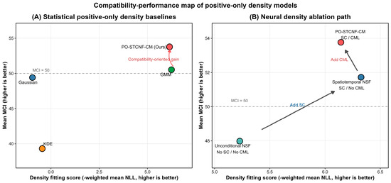
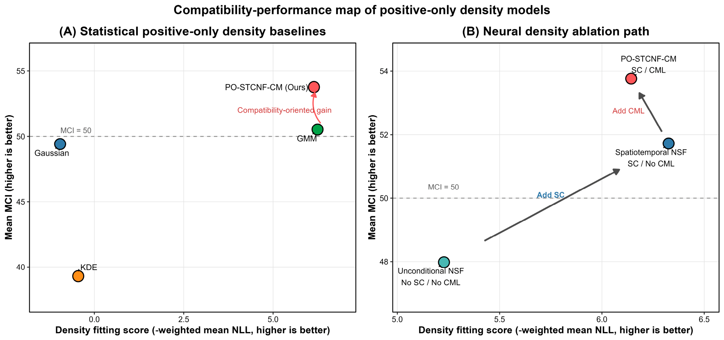
To examine the contributions of the proposed model components, an ablation analysis was conducted using neural spline flow (NSF) models [37]. Unconditional NSF estimated the meteorological distribution without contextual information, whereas Spatiotemporal NSF incorporated longitude, latitude, seasonal timing, and administrative-sector information. PO-STCNF-CM additionally included context-mismatch learning. The ablation results showed that introducing spatiotemporal conditioning reduced the mean NLL from −5.139 to −6.154 and the weighted mean NLL from −5.228 to −6.326 (Table 4). This improvement indicates that location and seasonal information contributed to the representation of LCF-associated meteorological conditions, supporting the use of context-dependent rather than a single context-independent meteorological distribution [43]. The relationship between likelihood-based density fitting and the model-specific MCI summaries is further illustrated descriptively in Figure 3.

Table 4. Ablation analysis of neural density models for evaluating spatiotemporal conditioning and context-mismatch learning.

Model	SC	CML	Mean NLL ↓	Median NLL ↓	Weighted Mean NLL ↓	Mean MCI ↑	Median MCI ↑	Coverage Error 80 ↓	Context Margin ↑
Unconditional NSF	×	×	−5.139	−5.594	−5.228	47.981	46.182	0.025	-
Spatiotemporal NSF	√	×	−6.154	−6.842	−6.326	51.724	52.886	0.037	5.020
PO-STCNF-CM (Ours)	√	√	−5.95	−6.919	−6.143	53.761	57.169	0.015	5.075

↓ indicates that lower values are better, while ↑ indicates that higher values are better. Bold values indicate the best performance in the table.

Figure 3. Relationship between density fitting and model-specific MCI summaries for positive-only density models. (A) Comparison between statistical positive-only density baselines and PO-STCNF-CM. (B) Neural density ablation path from Unconditional NSF to Spatiotemporal NSF and PO-STCNF-CM. The x-axis shows the density fitting score, calculated as the negative weighted mean NLL, where higher values indicate better density fitting. The y-axis shows mean MCI, where higher values indicate stronger meteorological compatibility. Red points denote PO-STCNF-CM.

Adding context-mismatch learning changed the balance of the evaluated metrics. PO-STCNF-CM produced a mean NLL of −5.949 compared with −6.154 for Spatiotemporal NSF, while its median NLL decreased from −6.842 to −6.919. PO-STCNF-CM also produced higher mean and median MCI values and a smaller 80% coverage error. The context likelihood margin increased from 5.020 for Spatiotemporal NSF to 5.075 for PO-STCNF-CM, indicating greater separation between the likelihoods assigned to observed and mismatched meteorological–context pairs. Together, these results suggest that context-mismatch learning strengthened context discrimination without improving all likelihood-based measures.

Overall, the model comparisons reveal complementary aspects of positive-only meteorological modelling. GMM provided the strongest likelihood fit among the statistical baselines, while the neural ablation showed that spatiotemporal conditioning substantially improved density fitting relative to the unconditional flow. Context-mismatch learning further increased the separation between observed and mismatched contexts and was associated with improved MCI calibration measures, although it did not further reduce mean or weighted mean NLL. PO-STCNF-CM was therefore used in the subsequent analyses to examine MCI distributions and the meteorological typicality of historical LCF records.

3.2. MCI-Based Meteorological Compatibility of Held-Out LCF Records

Following the model comparison, PO-STCNF-CM was applied to the chronologically held-out LCF records from 2022 to 2024 to generate event-level meteorological compatibility assessments for real historical fires. As defined in Section 2.2.3, the Meteorological Compatibility Index (MCI) expresses the relative typicality of a meteorological condition compared with historical LCF-associated conditions on a calibrated 0–100 scale [39]. Higher MCI values indicate greater similarity to meteorological conditions represented in the historical calibration records, whereas lower values indicate less typical conditions.

MCI describes meteorological compatibility rather than the probability of LCF occurrence [44]. Because the model was developed from observed LCF records without reliable non-fire samples, differences in MCI indicate differences in how typical the evaluated meteorological conditions are relative to historical LCF-associated conditions. Accordingly, a low MCI does not indicate that a fire could not occur; rather, it identifies an observed LCF event that occurred under meteorological conditions less commonly represented in the historical calibration data.

For descriptive interpretation, MCI values were grouped into four percentile-based compatibility categories (Table 5). Values of 80–100 were classified as highly compatible, values of 50–<80 as moderately compatible, values of 5–<50 as low or boundary compatibility, and values below 5 as strongly atypical. These categories were defined only to summarize relative positions on the calibrated MCI scale and should not be interpreted as operational fire-danger levels or occurrence-probability classes.

Table 5. Percentile-based interpretation of the Meteorological Compatibility Index.

MCI Range	Compatibility Category	Percentile-Based Interpretation	Meaning
MCI ≥ 80	High compatibility	Upper compatibility range relative to the calibration distribution	Meteorological conditions are strongly consistent with historical LCF-associated weather records.
50 ≤ MCI < 80	Moderate compatibility	Above the calibration median	Meteorological conditions are generally compatible with historical LCF-associated weather records.
5 ≤MCI < 50	Low or boundary compatibility	Below the calibration median	Meteorological conditions are less typical relative to historical LCF-associated weather records.
MCI < 5	Strongly atypical tail case	Extreme lower tail of the calibration scale	Meteorological conditions are rarely represented among historical LCF-associated records and require case-level interpretation.

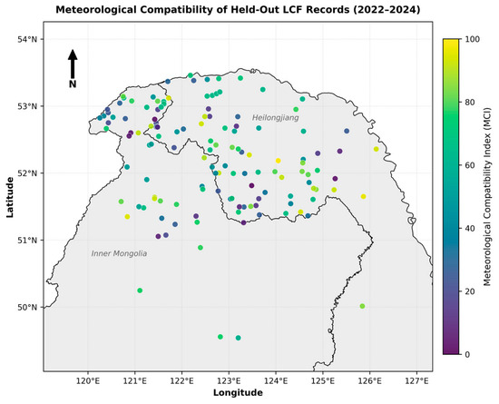
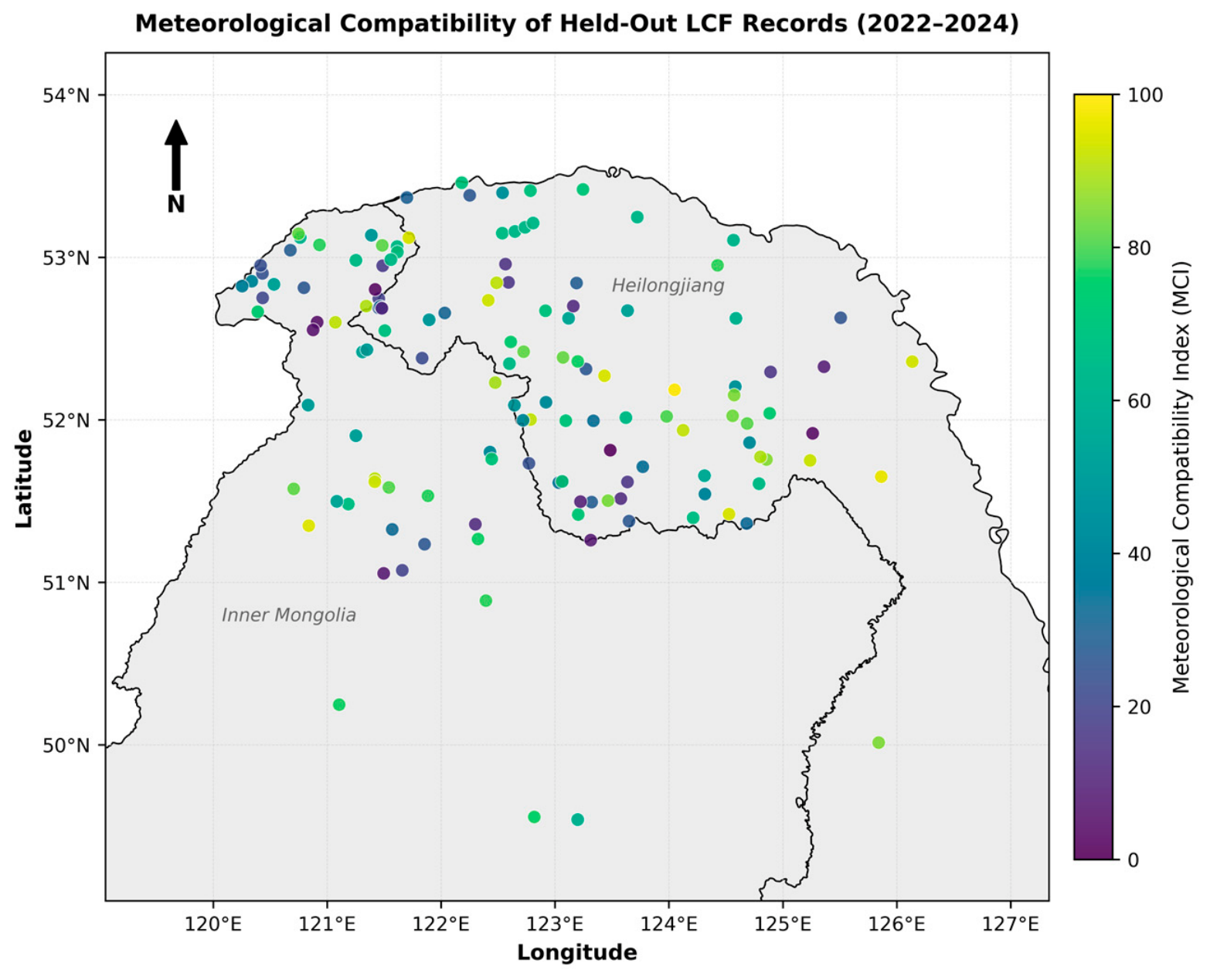
For the held-out LCF records, PO-STCNF-CM produced a mean MCI of 53.761 and a median MCI of 57.169. Both values were above 50, placing the central tendency of the held-out records within the moderate-compatibility range. This indicates that many LCF events from 2022–2024 occurred under meteorological conditions similar to those represented in the earlier historical records. At the same time, the distribution was not concentrated exclusively in the high-compatibility range, indicating substantial variation in meteorological typicality among individual LCF events. Based on the event-level MCI values averaged across the three repeated model runs, 31 of the 135 held-out events (23.0%) were classified as highly compatible (MCI ≥ 80), 47 (34.8%) as moderately compatible (50 ≤ MCI < 80), 53 (39.3%) as having low or boundary compatibility (5 ≤ MCI < 50), and 4 (3.0%) as strongly atypical (MCI < 5). These proportions further demonstrate that the held-out events spanned the full range of meteorological compatibility rather than being concentrated within a single category. To further present real assessed information rather than only summary metrics, the MCI values of the chronologically held-out LCF records were mapped according to their geographical locations (Figure 4). Each point represents a verified LCF event during 2022–2024, and its color indicates the mean MCI across repeated model runs. The spatial distribution shows that events with different levels of meteorological compatibility occurred across the study region, illustrating substantial event-level heterogeneity in the meteorological conditions associated with historical LCF occurrence. This map represents the spatial distribution of assessed MCI values among observed LCF events rather than a continuous spatial prediction of fire danger. It therefore provides event-level geographical evidence of how the proposed method evaluates the meteorological compatibility of real historical fires.

Figure 4. Spatial distribution of the Meteorological Compatibility Index (MCI) for chronologically held-out lightning-caused fire records during 2022–2024. Each point represents a verified LCF event, and the color indicates the mean MCI across repeated model runs. The map shows event-level meteorological compatibility rather than a continuous spatial prediction of fire danger.

Such variation is expected because meteorological conditions represent only part of the processes involved in LCF occurrence. Lightning activity, fuel and vegetation conditions, terrain, and other local factors can also influence whether lightning develops into a detectable fire. Previous studies have similarly shown that wildfire occurrence reflects interactions among climate, fuel, vegetation, and landscape characteristics [45]. Therefore, LCF records with low MCI values should not be regarded as erroneous or implausible events. Rather, they represent observed fires that occurred under meteorological conditions less commonly represented in the historical calibration data. These cases may reflect unusual meteorological conditions, local environmental variability, or factors not included in the present model.

The contextual formulation of PO-STCNF-CM further allows meteorological compatibility to vary with location and season. Because the conditional density incorporates longitude, latitude, seasonal timing, and administrative-sector information, similar meteorological conditions can have different MCI values under different spatial and seasonal contexts. This context dependence is consistent with previous studies reporting spatial and temporal heterogeneity in wildfire regimes and climate–fire relationships [46,47]. Accordingly, MCI reflects not only the similarity of meteorological variables to historical LCF-associated conditions, but also whether those conditions are typical of the corresponding spatial and seasonal context.

Overall, the held-out LCF records showed moderate meteorological compatibility on average, together with substantial variation among individual events. The MCI distribution therefore provides a way to distinguish commonly represented meteorological conditions from less typical conditions within the historical LCF record. These results provide the basis for the subsequent examination of LCF events across different MCI ranges.

3.3. Implications, Limitations, and Future Directions of Positive-Only LCF Compatibility Modelling

A central challenge in lightning-caused fires modelling is that the absence of a recorded fire does not necessarily constitute a reliable negative observation. Fire absence may reflect a lack of lightning ignition, unsuitable fuels, local terrain effects, limited detection, or reporting uncertainty. Consequently, directly constructed non-fire samples may introduce ambiguous labels into binary classification models [48]. The positive-only formulation avoids this uncertainty by characterizing meteorological conditions associated with observed LCF events rather than separating fire from non-fire conditions.

The main contribution of this study is therefore to formulate LCF meteorological assessment as a compatibility-modelling problem. PO-STCNF-CM evaluates how well a meteorological condition is represented by historical LCF-associated conditions under a given spatial and seasonal context, rather than estimating the absolute probability of fire occurrence. The Meteorological Compatibility Index (MCI) further converts density-based anomaly scores into a calibrated 0–100 scale, making the model output more interpretable than raw likelihood or negative log-likelihood values [44].

The model comparisons indicate that density fitting and meteorological compatibility capture different aspects of positive-only modelling. GMM provided strong likelihood fitting, whereas PO-STCNF-CM showed more favorable MCI and calibration-related results. The ablation analysis further showed that spatiotemporal conditioning improved density fitting, indicating that longitude, latitude, seasonal timing, and administrative-sector background contribute to characterizing the meteorological distribution of historical LCF records [45]. Context-mismatch learning additionally increased the context likelihood margin, although the improvement was modest, suggesting that explicit meteorological–context matching can complement conditional density estimation.

From an application perspective, MCI should be interpreted as a meteorological compatibility component rather than a standalone fire-occurrence probability. LCF occurrence also depends on lightning activity, fuel conditions, vegetation, terrain, ignition processes, and detection. MCI therefore provides a relative measure of how typical a meteorological condition is compared with historical LCF-associated conditions under similar spatial and seasonal contexts.

Several limitations should be considered. First, lightning ignition is a complex physical process that cannot be fully represented by meteorological variables alone [49]. A cloud-to-ground discharge may initiate ignition through localized Joule heating, heated particles or firebrands, or electrical-current propagation through tree and root systems, while subsequent combustion may remain latent or smouldering before developing into flaming fire [50]. These processes were not explicitly represented in the present statistical framework. Consequently, the recorded fire time may not coincide exactly with the initial lightning ignition time, and uncertainty may arise in linking the meteorological conditions at the recorded event time to the physical ignition process. In addition, the transition from lightning discharge to a detectable fire depends on fuel moisture, vegetation structure, topography, local fuel continuity, and other environmental conditions that were not explicitly modelled [20]. Second, the framework was developed from 984 historical LCF records in the Daxing’anling forest region, and MCI therefore depends on the representativeness of these records. Lightning characteristics, fuel moisture, vegetation structure, topography, and detection uncertainty were not explicitly modelled. In addition, MCI is a relative compatibility measure rather than P(fire|x, c), a classification metric, or an official fire-danger class.

Future research should extend the present framework by integrating temporally consistent lightning observations with fuel moisture, vegetation, topography, and other local environmental information. Particular attention should be given to delayed or holdover ignition processes and to the temporal relationship between lightning discharge, latent combustion, and fire detection [51]. Hybrid approaches combining data-driven modelling with physical knowledge of lightning ignition and fuel combustion may provide a more complete representation of the lightning-to-fire process. Validation across independent forest regions and climatic conditions will also be important for assessing the transferability and robustness of the proposed framework.

4. Conclusions

This study developed a positive-only framework for assessing the meteorological compatibility of lightning-caused fires (LCFs) using 984 historical LCF records from the Daxing’anling forest region, China. Rather than constructing uncertain non-fire samples or estimating fire occurrence probability, the proposed PO-STCNF-CM framework characterizes meteorological conditions associated with historical LCF events while accounting for spatial and seasonal context. The Meteorological Compatibility Index (MCI) further converts model-derived anomaly scores into an interpretable 0–100 compatibility scale.

The main findings and corresponding conclusions can be summarized as follows. (1) The positive-only formulation enabled meteorological compatibility to be assessed directly from verified historical LCF records without constructing potentially ambiguous non-fire samples, providing an alternative framework for situations in which reliable negative observations are unavailable. (2) GMM achieved the strongest likelihood fit among the statistical density baselines, indicating that LCF-associated meteorological conditions may require flexible multimodal representations rather than a single Gaussian distribution. (3) Ablation analysis showed that incorporating spatial and seasonal context improved density fitting relative to the unconditional neural flow, demonstrating that location and seasonal information are important for characterizing variations in LCF-associated meteorological conditions. (4) Context-mismatch learning increased the separation between observed and mismatched meteorological–context pairs and improved calibration-related performance, although it did not improve all likelihood-based metrics, indicating that its main contribution lies in strengthening contextual discrimination. (5) For the chronologically held-out LCF records from 2022 to 2024, PO-STCNF-CM produced a mean MCI of 53.761 and a median MCI of 57.169, with substantial variation among individual events. These results show that MCI provides an interpretable description of relative meteorological compatibility, but it should not be interpreted as an absolute probability of LCF occurrence or an official fire-danger class.

Future work should incorporate temporally consistent lightning observations, fuel and vegetation conditions, topography, delayed or holdover ignition processes, and other environmental information, while further evaluating the transferability and robustness of the framework across independent forest regions and climatic conditions.

References

- Janssen, T.A.J.; Jones, M.W.; Finney, D.; van der Werf, G.R.; van Wees, D.; Xu, W.; Veraverbeke, S. Extratropical forests increasingly at risk due to lightning fires. Nat. Geosci. 2023, 16, 1136–1144. [Google Scholar] [CrossRef] [Scilit]
- Pérez-Invernón, F.J.; Gordillo-Vázquez, F.J.; Huntrieser, H.; Jöckel, P. Variation of lightning-ignited wildfire patterns under climate change. Nat. Commun. 2023, 14, 739. [Google Scholar] [CrossRef] [Scilit] [PubMed]
- Gao, C.; Shi, C.; Li, J.; Yuan, S.; Huang, X.; Zhang, Q.; Ma, Q.; Wu, G. Igniting lightning, wildfire occurrence, and precipitation in the boreal forest of northeast China. Agric. For. Meteorol. 2024, 354, 110081. [Google Scholar] [CrossRef] [Scilit]
- Kalashnikov, D.A.; Abatzoglou, J.T.; Loikith, P.C.; Nauslar, N.J.; Bekris, Y.; Singh, D. Lightning-Ignited Wildfires in the Western United States: Ignition Precipitation and Associated Environmental Conditions. Geophys. Res. Lett. 2023, 50, e2023GL103785. [Google Scholar] [CrossRef] [Scilit]
- Stepanian, P.M.; Williams, E.R. Extinguishing the Fiery Skies: The History and Modern Prospects of Lightning Suppression within Thunderstorms. Bull. Am. Meteorol. Soc. 2024, 105, E1977–E1988. [Google Scholar] [CrossRef] [Scilit]
- Alkhatib, R.; Sahwan, W.; Alkhatieb, A.; Schütt, B. A Brief Review of Machine Learning Algorithms in Forest Fires Science. Appl. Sci. 2023, 13, 8275. [Google Scholar] [CrossRef] [Scilit]
- Ku, C.-Y.; Lu, H.-C.; Tu, Y.-T.; Liu, C.-Y. Charactering Human-Caused Fires Using GIS-Based Dimensionality Reduction Techniques in Keelung City, Taiwan. Appl. Sci. 2024, 14, 1930. [Google Scholar] [CrossRef] [Scilit]
- Cilli, R.; Elia, M.; D’Este, M.; Giannico, V.; Amoroso, N.; Lombardi, A.; Pantaleo, E.; Monaco, A.; Sanesi, G.; Tangaro, S.; et al. Explainable artificial intelligence (XAI) detects wildfire occurrence in the Mediterranean countries of Southern Europe. Sci. Rep. 2022, 12, 16349. [Google Scholar] [CrossRef] [Scilit] [PubMed]
- Bouzeraa, Y.; Bouchemal, N.; Djaaboub, S.; Hristov, G.; Zahariev, P. Machine Learning-Based Wildfire Susceptibility Mapping: A GIS-Integrated Predictive Framework. Appl. Sci. 2025, 15, 12188. [Google Scholar] [CrossRef] [Scilit]
- Zheng, S.; Gao, P.; Wang, W.; Zou, X. A Highly Accurate Forest Fire Prediction Model Based on an Improved Dynamic Convolutional Neural Network. Appl. Sci. 2022, 12, 6721. [Google Scholar] [CrossRef] [Scilit]
- Zacharakis, I.; Tsihrintzis, V.A. Integrated wildfire danger models and factors: A review. Sci. Total Environ. 2023, 899, 165704. [Google Scholar] [CrossRef] [Scilit] [PubMed]
- Xie, X.; Ning, W.; Huang, Y.; Li, Z.; Yu, S.; Yang, H. Graph-based Bayesian network conditional normalizing flows for multiple time series anomaly detection. Int. J. Intell. Syst. 2022, 37, 10924–10939. [Google Scholar] [CrossRef] [Scilit]
- Andrianarivony, H.S.; Akhloufi, M.A. Machine Learning and Deep Learning for Wildfire Spread Prediction: A Review. Fire 2024, 7, 482. [Google Scholar] [CrossRef] [Scilit]
- Zacharakis, I.; Tsihrintzis, V.A. Environmental Forest Fire Danger Rating Systems and Indices around the Globe: A Review. Land 2023, 12, 194. [Google Scholar] [CrossRef] [Scilit]
- Jolly, W.M.; Freeborn, P.H.; Bradshaw, L.S.; Wallace, J.; Brittain, S. Modernizing the US National Fire Danger Rating System (version 4): Simplified fuel models and improved live and dead fuel moisture calculations. Environ. Model. Softw. 2024, 181, 106181. [Google Scholar] [CrossRef] [Scilit]
- Coughlan, R.; Di Giuseppe, F.; Vitolo, C.; Barnard, C.; Lopez, P.; Drusch, M. Using machine learning to predict fire-ignition occurrences from lightning forecasts. Meteorol. Appl. 2021, 28, e1973. [Google Scholar] [CrossRef] [Scilit]
- Di Giuseppe, F. The Value of Probabilistic Prediction for Lightning Ignited Fires. Geophys. Res. Lett. 2022, 49, e2022GL099669. [Google Scholar] [CrossRef] [Scilit]
- Tang, X.; Machimura, T.; Li, J.; Yu, H.; Liu, W. Evaluating Seasonal Wildfire Susceptibility and Wildfire Threats to Local Ecosystems in the Largest Forested Area of China. Earth’s Future 2022, 10, e2021EF002199. [Google Scholar] [CrossRef] [Scilit]
- Rao, K.; Williams, A.P.; Diffenbaugh, N.S.; Yebra, M.; Bryant, C.; Konings, A.G. Dry Live Fuels Increase the Likelihood of Lightning-Caused Fires. Geophys. Res. Lett. 2023, 50, e2022GL100975. [Google Scholar] [CrossRef] [Scilit]
- Wickramasinghe, A.M.K.; Boer, M.M.; Cunningham, C.X.; Nolan, R.H.; Bowman, D.M.J.S.; Williamson, G.J. Modeling the Probability of Dry Lightning-Induced Wildfires in Tasmania: A Machine Learning Approach. Geophys. Res. Lett. 2024, 51, e2024GL110381. [Google Scholar] [CrossRef] [Scilit]
- Zhang, Q.; Gao, C.; Shi, C. An improved machine-learning model for lightning-ignited wildfire prediction in Texas. Environ. Res. Lett. 2025, 20, 64026. [Google Scholar] [CrossRef] [Scilit]
- Lee, J.; Shin, J.; Lee, J.; Park, C.; Sohn, D. Development of a Data-Based Machine Learning Model for Classifying and Predicting Property Damage Caused by Fire. Appl. Sci. 2023, 13, 11866. [Google Scholar] [CrossRef] [Scilit]
- Shirazi, Z.; Wang, L.; Bondur, V.G. Modeling Conditions Appropriate for Wildfire in South East China—A Machine Learning Approach. Front. Earth Sci. 2021, 9, 622307. [Google Scholar] [CrossRef] [Scilit]
- Ismail, F.N.; Woodford, B.J.; Licorish, S.A.; Miller, A.D. An assessment of existing wildfire danger indices in comparison to one-class machine learning models. Nat. Hazards 2024, 120, 14837–14868. [Google Scholar] [CrossRef] [Scilit]
- Li, F.; Dong, S.; Leier, A.; Han, M.; Guo, X.; Xu, J.; Wang, X.; Pan, S.; Jia, C.; Zhang, Y.; et al. Positive-unlabeled learning in bioinformatics and computational biology: A brief review. Brief. Bioinform. 2022, 23, bbab461. [Google Scholar] [CrossRef] [Scilit]
- Song, L.; Estes, L. itsdm: Isolation forest-based presence-only species distribution modelling and explanation in r. Methods Ecol. Evol. 2023, 14, 831–840. [Google Scholar] [CrossRef] [Scilit]
- Xu, Y.; Ma, Y.; Ye, Q.; Fu, L.; Yang, X. Interpretable deep one-class model for forest fire detection. Expert Syst. Appl. 2025, 281, 127657. [Google Scholar] [CrossRef] [Scilit]
- Valavi, R.; Guillera-Arroita, G.; Lahoz-Monfort, J.J.; Elith, J. Predictive performance of presence-only species distribution models: A benchmark study with reproducible code. Ecol. Monogr. 2022, 92, e01486. [Google Scholar] [CrossRef] [Scilit]
- Smith, J.R.; Levine, J.M. Linking relative suitability to probability of occurrence in presence-only species distribution models: Implications for global change projections. Methods Ecol. Evol. 2025, 16, 854–865. [Google Scholar] [CrossRef] [Scilit]
- Rausell-Moreno, A.; Galiana, N.; Naimi, B.; Araújo, M.B. Improving species distribution models by optimising background points: Impacts on current and future climate projections. Ecol. Model. 2025, 507, 111177. [Google Scholar] [CrossRef] [Scilit]
- Lee, C.W.; Leveugle, S.; Grouchy, P.; Langley, C.; Stolpner, S.; Kelly, J.; Waslander, S.L. FlowCLAS: Enhancing Normalizing Flow-Based Anomaly Segmentation Via Contrastive Learning. In Proceedings of the IEEE/CVF Winter Conference on Applications of Computer Vision (WACV); IEEE: Piscataway, NJ, USA, 2026; pp. 6998–7007. [Google Scholar]
- Illarionova, S.; Shadrin, D.; Gubanov, F.; Shutov, M.; Tasuev, U.; Evteeva, K.; Mironenko, M.; Burnaev, E. Exploration of geo-spatial data and machine learning algorithms for robust wildfire occurrence prediction. Sci. Rep. 2025, 15, 10712. [Google Scholar] [CrossRef] [Scilit]
- Chen, K.; Xiao, J.; Liu, Q.; Huang, Z.; Ji, C.; Ji, K. Robust multivariate time series anomaly detection via conditional normalizing flow with patch embedding and cross time attention. Auton. Transp. Res. 2026, 2, 96–110. [Google Scholar] [CrossRef] [Scilit]
- Guan, S.; He, Z.; Ma, S.; Gao, M. Conditional normalizing flow for multivariate time series anomaly detection. ISA Trans. 2023, 143, 231–243. [Google Scholar] [CrossRef] [Scilit] [PubMed]
- Gudovskiy, D.; Ishizaka, S.; Kozuka, K. CFLOW-AD: Real-Time Unsupervised Anomaly Detection with Localization via Conditional Normalizing Flows. In 2022 IEEE/CVF Winter Conference on Applications of Computer Vision (WACV); IEEE: Piscataway, NJ, USA, 2022; pp. 1819–1828. [Google Scholar]
- Papamakarios, G.; Nalisnick, E.; Rezende, D.J.; Mohamed, S.; Lakshminarayanan, B. Normalizing Flows for Probabilistic Modeling and Inference. J. Mach. Learn. Res. 2021, 22, 2617–2680. [Google Scholar]
- Durkan, C.; Bekasov, A.; Murray, I.; Papamakarios, G. Neural Spline Flows. In Advances in Neural Information Processing Systems; Wallach, H., Larochelle, H., Beygelzimer, A., Alché-Buc, F.d., Fox, E., Garnett, R., Eds.; Curran Associates, Inc.: Red Hook, NY, USA, 2019. [Google Scholar]
- Khosla, P.; Teterwak, P.; Wang, C.; Sarna, A.; Tian, Y.; Isola, P.; Maschinot, A.; Liu, C.; Krishnan, D. Supervised Contrastive Learning. In Advances in Neural Information Processing Systems; Larochelle, H., Ranzato, M., Hadsell, R., Balcan, M.F., Lin, H., Eds.; Curran Associates, Inc.: Red Hook, NY, USA, 2020; pp. 18661–18673. [Google Scholar]
- Angelopoulos, A.N.; Bates, S. Conformal Prediction: A Gentle Introduction. Found. Trends Mach. Learn. 2023, 16, 494–591. [Google Scholar] [CrossRef] [Scilit]
- Garg, I.; Majumder, S. On the Integration of Cross-Conformal Prediction, Ensembles, and Sampling for Uncertainty Quantification in One-Class Anomaly Detection. In Proceedings of the Fourteenth Symposium on Conformal and Probabilistic Prediction with Applications; Nguyen, K.A., Luo, Z., Papadopoulos, H., Löfström, T., Carlsson, L., Boström, H., Eds.; PMLR: Egham, UK, 2025; pp. 687–705. [Google Scholar]
- Cerqueira, V.; Torgo, L.; Mozetič, I. Evaluating time series forecasting models: An empirical study on performance estimation methods. Mach. Learn. 2020, 109, 1997–2028. [Google Scholar] [CrossRef] [Scilit]
- Loshchilov, I.; Hutter, F. Decoupled Weight Decay Regularization. In Proceedings of the 7th International Conference on Learning Representations (ICLR 2019), New Orleans, LA, USA, 6–9 May 2019. [Google Scholar]
- Liu, J.; Wang, Y.; Guo, H.; Lu, Y.; Xu, Y.; Sun, Y.; Gan, W.; Sun, R.; Li, Z. Spatial and temporal patterns and driving factors of forest fires based on an optimal parameter-based geographic detector in the Panxi region, Southwest China. Fire Ecol. 2024, 20, 27. [Google Scholar] [CrossRef] [Scilit]
- Guillera-Arroita, G.; Lahoz-Monfort, J.J.; Elith, J.; Gordon, A.; Kujala, H.; Lentini, P.E.; McCarthy, M.A.; Tingley, R.; Wintle, B.A. Is my species distribution model fit for purpose? Matching data and models to applications. Glob. Ecol. Biogeogr. 2015, 24, 276–292. [Google Scholar] [CrossRef] [Scilit]
- Jones, M.W.; Abatzoglou, J.T.; Veraverbeke, S.; Andela, N.; Lasslop, G.; Forkel, M.; Smith, A.J.P.; Burton, C.; Betts, R.A.; van der Werf, G.R.; et al. Global and Regional Trends and Drivers of Fire Under Climate Change. Rev. Geophys. 2022, 60, e2020RG000726. [Google Scholar] [CrossRef] [Scilit]
- Parks, S.A.; Holsinger, L.M.; Voss, M.A.; Loehman, R.A.; Robinson, N.P. Mean Composite Fire Severity Metrics Computed with Google Earth Engine Offer Improved Accuracy and Expanded Mapping Potential. Remote Sens. 2018, 10, 879, Correction in Remote Sens. 2021, 13, 4580. https://doi.org/10.3390/rs13224580. [Google Scholar] [CrossRef] [Scilit]
- Di Virgilio, G.; Evans, J.P.; Blake, S.A.P.; Armstrong, M.; Dowdy, A.J.; Sharples, J.; McRae, R. Climate Change Increases the Potential for Extreme Wildfires. Geophys. Res. Lett. 2019, 46, 8517–8526. [Google Scholar] [CrossRef] [Scilit]
- Barbet-Massin, M.; Jiguet, F.; Albert, C.H.; Thuiller, W. Selecting pseudo-absences for species distribution models: How, where and how many? Methods Ecol. Evol. 2012, 3, 327–338. [Google Scholar] [CrossRef] [Scilit]
- Song, Y.; Xu, C.; Li, X.; Oppong, F. Lightning-Induced Wildfires: An Overview. Fire 2024, 7, 79. [Google Scholar] [CrossRef] [Scilit]
- Pineda, N.; Altube, P.; Alcasena, F.J.; Casellas, E.; Segundo, H.S.; Montanyà, J. Characterising the holdover phase of lightning-ignited wildfires in Catalonia. Agric. For. Meteorol. 2022, 324, 109111. [Google Scholar] [CrossRef] [Scilit]
- Moris, J.V.; Ascoli, D.; Hunt, H.G.P. Survival functions of holdover time of lightning-ignited wildfires. Electr. Power Syst. Res. 2024, 231, 110296. [Google Scholar] [CrossRef] [Scilit]
Disclaimer/Publisher’s Note: The statements, opinions and data contained in all publications are solely those of the individual author(s) and contributor(s) and not of MDPI and/or the editor(s). MDPI and/or the editor(s) disclaim responsibility for any injury to people or property resulting from any ideas, methods, instructions or products referred to in the content. |
© 2026 by the authors. Licensee MDPI, Basel, Switzerland. This article is an open access article distributed under the terms and conditions of the Creative Commons Attribution (CC BY) license.