


Abstract
Limited labeled data and overlapping multisensor signatures make liquid rocket engine fault classification challenging, particularly when feature fusion introduces redundant information. This study proposes a multi-scale feature fusion framework with a calibrated convex ensemble (CCE). A 684-dimensional multi-window statistical representation is fused with a 32-dimensional temporal bottleneck learned through multi-scale convolution, channel attention, and bidirectional long short-term memory. Random-forest-based recursive feature elimination selects features within training partitions, while calibrated predictions from four heterogeneous classifiers are aggregated using simplex-constrained weights. Evaluation focuses on 1106 simulated sequences representing nine known faults in XJTU-REF; the three healthy sequences are excluded from the primary task. Five repetitions of five-fold nested cross-validation yield an accuracy of 90.16 ± 1.04%, a macro-F1 score of 89.84 ± 1.08%, and a Matthews correlation coefficient of 0.891 ± 0.012 (mean ± standard deviation across outer-test folds). Accuracy exceeds that of the random-forest baseline using mean features from the final 20% of each sequence by 2.45 percentage points. Ablations support the complementary roles of the two representations and feature selection, while calibration reduces expected calibration error from 7.18% to 3.76% relative to the uncalibrated ensemble. Leave-one-unit-out accuracy is 86.26 ± 1.21% across three simulated units, indicating lower performance on unseen units than under sample-level validation. These findings support complementary feature fusion with dimensionality control and calibrated aggregation for closed-set fault classification, while healthy-state recognition and real-engine applicability require further validation.
1. Introduction
Reliable fault classification is an important component of liquid rocket engine (LRE) diagnostic analysis, providing a basis for identifying suspect subsystems and guiding subsequent engineering assessment. The coupled behavior of engine subsystems produces multisensor responses in which persistent operating-level deviations coexist with localized temporal changes. Consequently, diagnostically useful information may be distributed across different variables and temporal scales rather than concentrated in a single measurement or observation interval. Different fault mechanisms can also produce similar pressure and flow responses, making their separation dependent on subtle differences in signal magnitude, fluctuation, and temporal evolution. Learning these distinctions from a limited number of labeled engine sequences therefore requires a careful balance between representational richness and model complexity.
Existing LRE-specific studies have explored several approaches to this problem, including model-based filtering [1], small-sample Bayesian classification [2], and neural sequence representations [3]. Model-based methods exploit prescribed system dynamics, but their diagnostic interpretation remains dependent on the adequacy of the underlying model and its assumptions. Bayesian methods provide a framework for learning under limited observations, whereas neural sequence models offer flexible representations of nonlinear temporal relationships. These approaches address important aspects of LRE diagnosis, but they do not eliminate the trade-offs associated with representation design and finite-sample learning. In particular, a compact representation may omit useful fault information, while a more expressive representation can introduce additional estimation uncertainty. The challenge addressed in this study is to exploit complementary signal characteristics without allowing the resulting model complexity to exceed what the available labeled data can support.
A first challenge concerns the incomplete characterization of fault signatures by a single representation. Statistical descriptors summarize operating levels, variability, distributional shape, and local changes, but they do not explicitly preserve the complete temporal ordering of a sequence. Restricting these descriptors to one observation window can further obscure differences between persistent deviations and localized responses. Learned temporal representations can capture ordering and contextual dependencies, but a temporal-only model must infer useful discriminative structure from the available training sequences. Combining these two forms of information is therefore attractive, but their complementarity does not guarantee that direct concatenation will improve classification. Correlated statistical descriptors and weakly informative learned coordinates can enlarge the feature space without providing a corresponding increase in usable information. For small-sample LRE classification, feature fusion must consequently be accompanied by explicit dimensionality control.
A second challenge concerns the reliability of the final decision. Classification accuracy alone does not establish whether predicted probabilities appropriately reflect the frequency of correct decisions. This distinction is particularly relevant when fault categories have overlapping signatures. Moreover, heterogeneous classifiers produce outputs with different probabilistic characteristics, so direct soft voting can combine predictions that are not equally calibrated. Probability-calibration studies have demonstrated the importance of evaluating and correcting such discrepancies [4]. A suitable decision mechanism should therefore address both discrimination and probability quality, rather than assuming that a higher classification score necessarily implies more reliable confidence estimates. It should also estimate ensemble weights from training-derived predictions instead of relying solely on manually specified voting preferences.
A third challenge is to distinguish improvements in model performance from effects introduced by model selection and data partitioning. Feature extraction, feature selection, calibration, and ensemble-weight estimation are all data-dependent operations. Their placement within the validation procedure determines whether the resulting performance estimates reflect genuinely held-out observations. In addition, sample-level and engine-unit-level evaluations answer different questions: a random stratified split can assess classification of additional sequences from represented units, whereas holding out an entire engine unit evaluates transfer to a unit excluded from model development. These distinctions are essential when assessing a multistage framework with numerous tunable components and only a small number of simulated engine units.
To address these challenges, this paper proposes a multi-scale feature fusion framework with a calibrated convex ensemble (CCE). The statistical branch constructs a 684-dimensional representation from multiple temporal windows, preserving complementary descriptions of operating levels, distributional characteristics, and local variation. In parallel, a temporal branch combines multi-scale convolution, squeeze-and-excitation channel attention, and bidirectional recurrence to produce a compact 32-dimensional bottleneck. The resulting 716-dimensional representation is refined through random-forest-based recursive feature elimination (RF-RFE), following the recursive feature-selection principle [5]. The retained dimension and model settings are selected within the inner training procedure. Finally, Random Forest, Support Vector Machine, Gradient Boosting, and K-Nearest Neighbors predictions are calibrated and combined using nonnegative weights constrained to the probability simplex. The design thus links complementary representation, finite-sample complexity control, and probability-level decision fusion within a common training-partition framework.
The framework is evaluated on XJTU-REF, which provides simulated multisensor sequences generated from an open-cycle LRE model [6]. The dataset contains 1106 sequences across nine fault conditions but only three healthy sequences. Accordingly, the primary task is closed-set classification among the nine modeled faults, conditional on the input belonging to this fault set. Healthy-state recognition and the probability that an arbitrary operational sequence is faulty are outside the evaluated task. Repeated nested cross-validation and leave-one-unit-out evaluation are reported separately to distinguish sample-level performance from transfer across simulated engine units.
The main contributions of this study are as follows:
- A problem-specific dual-view representation. We combine multi-window statistical descriptors with a compact learned temporal representation to characterize persistent operating deviations and temporal fault patterns within the same sequence. Single-view and fused configurations provide explicit comparisons for assessing whether these representations contribute complementary classification information.
- Training-partition-controlled feature fusion and selection. We incorporate RF-RFE into the inner model-selection procedure so that the retained representation is determined without accessing the outer-test data. Comparing direct concatenation with selected fusion separates the effect of adding features from the effect of controlling their finite-sample complexity.
- A calibrated heterogeneous decision formulation. We calibrate training-derived cross-fitted outputs from four complementary classifiers and estimate their ensemble weights by minimizing a regularized class-balanced log-loss over the probability simplex. This formulation replaces manually assigned voting weights with a defined optimization objective and permits separate assessment of classification performance and probability quality.
- An evaluation that separates component effects and generalization targets. We combine repeated nested validation, component ablations, paired comparisons, and individual engine-unit holdouts to examine representation, selection, and decision-stage contributions. The resulting evidence is interpreted specifically for nine-fault classification on the simulated benchmark, with sample-level results distinguished from cross-unit transfer.
2. Related Work and Scope of the Contribution
2.1. LRE-Specific Evidence
Fault diagnosis for liquid rocket engines (LREs) has been pursued through model-based, knowledge-based, and data-driven paradigms. Model-based approaches, such as Kalman filtering and particle filtering, offer interpretable residuals but suffer from high dependency on accurate physical models and poor generalizability [7,8,9]. Knowledge-driven expert systems encode human rules or fuzzy logic but struggle with coupled fault relationships and inference efficiency [10,11]. Traditional signal processing techniques, e.g., frequency analysis, parity-space methods, and wavelet denoising, have been applied but require extensive domain expertise and perform poorly under noisy or non-stationary conditions [12,13,14]. With advances in AI, intelligent data-driven methods have gained traction. Conventional machine learning models (SVM, ANN, random forests) combined with hand-crafted features have been used for turbopump and steady-state fault detection [15,16,17,18,19,20], while deep learning architectures such as CNNs, LSTMs, and autoencoders enable end-to-end feature learning and classification [21,22,23,24].
To overcome the critical bottleneck of limited fault-labeled data, researchers have developed data resampling and generation techniques (SMOTE, GANs, VAEs, digital twins) [25,26,27,28,29,30,31], feature-level enhancements via attention and regularization [32,33,34,35,36], and algorithm-level solutions including cost-sensitive learning and ensemble classifiers [37,38,39]. Transfer learning leverages source-domain knowledge for new engines with sparse target data [40], while meta-learning and zero-shot learning are emerging for few-shot and unseen fault scenarios [41,42]. Despite these progresses, challenges remain in developing comprehensive frameworks, understanding deep model theory, and effectively integrating domain knowledge (e.g., physical causality and failure rules) with data-driven models to ensure interpretability and trustworthiness, issues that recent XAI methods like SHAP and LIME have begun to address but lack systematic evaluation.
2.2. General Methodological Foundations
Squeeze-and-excitation reweights learned channels, while RFE is a general feature-selection procedure [5]. Neither establishes physical sensor causality. Probability calibration has its own evaluation objectives [4]; a classifier can improve NLL without materially changing its predicted labels. Selection stability requires an explicit resampling definition and attention to subset size [43]. Modern time-series methods such as InceptionTime and ROCKET provide useful additional comparators [44,45]. The positioning of the study is shown in Table 1.
Table 1.
Positioning of the study. Differences describe scope, not an audited absence of capabilities in earlier work.
3. Proposed Methodology
3.1. Overview of the Proposed Framework
Figure 1 illustrates the complete learning and evaluation pipeline of the proposed framework. Given a multivariate liquid rocket engine sequence, sensor-wise normalization is first estimated exclusively from the current training partition. The normalized sequence is then processed through two complementary representation branches. The statistical branch extracts a 684-dimensional descriptor from four nested temporal windows to characterize operating levels, distributional properties, and local variations. In parallel, the temporal branch learns a 32-dimensional bottleneck representation through multi-scale convolution, latent-channel attention, bidirectional recurrence, and an auxiliary classification objective. The two representations are concatenated into a 716-dimensional dual-view feature vector, which is robustly scaled and reduced through Random-Forest-based recursive feature elimination (RF-RFE). The retained feature dimension and all remaining hyperparameters are selected entirely within the inner cross-validation loop.
Figure 1.
Overall architecture of the proposed leakage-controlled dual-view fault-diagnosis framework.
The selected representation is subsequently supplied to four heterogeneous base classifiers: Random Forest (RF), radial-basis-function Support Vector Machine (RBF-SVM), Gradient Boosting (GB), and distance-weighted K-Nearest Neighbors (KNN). Their cross-fitted score vectors are individually calibrated and combined through simplex-constrained convex weight optimization. Every data-dependent operation, including normalization, representation learning, robust scaling, feature selection, probability calibration, and ensemble-weight estimation, is refitted using only the corresponding training partition. Repeated nested cross-validation evaluates sample-level generalization, whereas leave-one-unit-out evaluation measures transfer to an unseen simulated engine unit. The framework therefore addresses three related questions: whether the statistical and temporal views contain complementary diagnostic information, whether nested dimensionality control reduces the finite-sample variance introduced by feature fusion, and whether calibrated ensemble learning improves the reliability of the final predictive distribution.
3.2. Problem Formulation and Notation
We first define the principal notation in Table 2. Let the complete benchmark be represented by
where is the ith multisensor sequence, is the number of time samples, is the number of monitored variables, is the operating-condition label, and identifies the simulated engine unit from which the sequence is generated.
Table 2.
Principal notation used in the proposed methodology.
Because the benchmark contains only three healthy observations, the primary analysis is conducted on the fault-only subset
with
The ten-class task including the healthy condition is retained only as an exploratory analysis and is not used to support claims concerning healthy-state recognition.
The diagnostic model maps an input sequence to the probability simplex
The predicted class is
For a generic training index set , the supervised temporal extractor is trained by minimizing the class-balanced empirical cross-entropy
where
The downstream RF, RBF-SVM, GB, and KNN models retain their respective training objectives. Class weighting is applied to a downstream learner only when it is supported by that learner and included in the corresponding candidate configuration. The class-balanced negative log-likelihood is also used in the probability-level ensemble-weight optimization introduced in Section 3.7.
Assumption 1
(Evaluation isolation). For every outer split, the outer-test partition is excluded from sensor normalization, temporal-network training, early stopping, feature scaling, RF-RFE, hyperparameter selection, probability calibration, ensemble-weight estimation, and all other data-dependent operations. The outer-test partition is accessed only after the complete model-development procedure has been finalized on the corresponding outer-training partition.
3.3. Training-Partition Sensor Normalization
Sensor normalization is performed using statistics estimated from the current fitting partition rather than independently within each sample. Let denote the training indices available to a particular fitting operation. For sensor d, the training-partition mean and variance are
Any training, validation, or test sequence transformed by this fitted normalizer is represented as
where is a small numerical constant.
This training-partition transformation preserves between-sample deviations relative to the fitted operating distribution. Such deviations are diagnostically meaningful for pressure, flow, power, mixture-ratio, and temperature-related variables. In contrast, fitting a separate scaler to each individual sequence would force every sensor trajectory to have approximately zero mean and unit variance, thereby attenuating absolute operating-level differences that the statistical representation is intended to retain.
3.4. Multi-Scale Statistical View
The statistical view describes operating levels, distributional shape, and local temporal variation over nested horizons. The window set is
For , define
and
At 500 Hz, the four windows correspond approximately to the complete one-second record and its final 0.50, 0.30, and 0.15 s segments.
For sample i, sensor d, and window w, the local mean and standard deviation are
The skewness and excess kurtosis are
Let
The mean and standard deviation of the first-order differences are
Together with the minimum, maximum, and median, the nine-dimensional sensor-window descriptor is
The complete statistical representation is
where ⨁ denotes vector concatenation.
The nested windows encode a controlled bias–variance trade-off. Long windows provide relatively stable estimates of persistent operating shifts, whereas short windows increase sensitivity to localized late-stage transients. The different horizons are therefore treated as complementary statistical views of the same sequence rather than as independent observations.
3.5. Learned Temporal View
The statistical representation does not retain the complete ordering of samples within each window; first-difference descriptors retain only limited local-order information. A learned temporal branch is therefore introduced to model local temporal motifs, longer-range dependencies, and interactions between latent dynamic channels.
3.5.1. Multi-Scale Convolutional Representation
Let
be the set of convolutional kernel sizes. For sample i and branch ,
where , each branch contains filters, ∗ denotes same-padded one-dimensional convolution along the temporal dimension, and max pooling has width and stride two. At 500 Hz, the three kernels span approximately 6, 14, and 30 ms, respectively.
The branch outputs are concatenated along the latent-channel dimension:
3.5.2. Latent-Channel Attention
The attention module reweights the 96 convolutional latent channels rather than the 19 original sensor variables. Temporal squeeze pooling produces
The latent-channel weights are
where
corresponding to a reduction ratio of four. The attended representation is
where ⊙ denotes element-wise multiplication.
Because the attention coefficients act after convolutional feature generation, they should not be interpreted as direct physical importance scores for individual sensors. Sensor-level interpretation requires a separate attribution analysis with respect to the original input variables.
3.5.3. Bidirectional Recurrence and Bottleneck Projection
A bidirectional LSTM with 32 hidden units per direction processes . Its pooled representation is
A complementary unidirectional LSTM with 32 hidden units is applied directly to the normalized sensor sequence:
The two recurrent representations are concatenated and projected through a two-layer bottleneck:
The 32-dimensional vector is the temporal representation used in the subsequent feature-fusion stage.
During representation learning, an auxiliary classification head is attached:
The temporal extractor is optimized using Equation (6). During inner-loop model development, the epoch number is selected using an early-stopping subset drawn exclusively from the corresponding inner-training partition. The inner-validation fold used for configuration scoring is not used for early stopping. Once the epoch number has been selected, the auxiliary head is discarded and Equation (33) is used as the temporal feature map.
3.6. Feature Fusion, Robust Scaling, and Nested Selection
The statistical and temporal views are concatenated as
For every fused coordinate j, a robust transformation is fitted from the current training partition :
The same fitted median and interquartile range are subsequently applied to the associated validation or test partition.
RF-RFE recursively removes weak fused coordinates. For tree b and split node n, let denote the feature used at that node, the proportion of training samples reaching the node, and its Gini impurity. The weighted impurity reduction is
The forest importance assigned to feature j is
Starting from
one elimination operation is
In implementation, multiple lowest-ranked variables may be removed per iteration to reduce computational cost, provided that the removal schedule is fixed before accessing the corresponding validation fold.
For the complete 716-D representation, the retained dimension is selected from
For inner fold r, let denote the q-feature subset obtained exclusively from that fold’s inner-training partition. The selected dimension satisfies
For an ablation with fewer input coordinates, infeasible candidate dimensions are excluded. Ties are resolved by lower mean inner negative log-likelihood and then lower mean expected calibration error. In the complete search procedure, q is treated as one component of the candidate configuration and is therefore selected jointly with the remaining hyperparameters.
For an aligned statistical-feature dictionary, feature-selection stability across training resamples is summarized by the mean pairwise Jaccard index
This diagnostic is computed only from training-derived subsets of the fixed 684-coordinate statistical dictionary. Independently trained temporal coordinates cannot be assumed to have aligned identities; their retention is summarized at block level. Subset-size effects and a chance-adjusted statistic are discussed in Section 5.3. No numerical stability estimate is claimed without the corresponding selection archive.
The selected representation supplied to every base classifier is
Proposition 1
(Information monotonicity of the fused view). Let
and define
Under zero–one loss,
Proof.
The Bayes risks based on U and are
Conditioning on U gives
where the inequality follows from the convexity of the maximum operator and the equality follows from the tower property. Taking expectations yields Equation (47). □
Proposition 1 establishes that observing the temporal view cannot increase the Bayes-optimal classification risk because a theoretically optimal classifier can always ignore the additional view. However, it does not imply that arbitrary empirical concatenation must improve finite-sample performance. With limited samples, redundant or weak coordinates can increase estimation variance and degrade a misspecified classifier. This distinction provides the theoretical motivation for nested scaling and RF-RFE after dual-view concatenation.
3.7. Calibrated Convex Ensemble
The selected representation is supplied to
heterogeneous base learners: RF, RBF-SVM, GB, and distance-weighted KNN. These learners provide different inductive biases. RF and GB construct piecewise nonlinear tree partitions, RBF-SVM produces a smooth kernel-induced decision boundary, and KNN preserves local neighborhood structure.
Let
denote the raw score or uncalibrated probability vector produced by learner m. A calibration mapping
produces
Temperature scaling is considered when a compatible logit vector is available; Platt-type scaling and isotonic regression are considered for classifiers providing decision scores or empirical probabilities. The calibration family is selected in the inner loop using cross-fitted probabilities and validation NLL, and the calibrated multiclass vector is renormalized when required [4].
Let
be the calibrated probability assigned by learner m to class c for cross-fitted observation i. The ensemble weights are estimated by
The probability-simplex constraint prevents negative voting coefficients and makes the final output a valid convex combination of calibrated probability vectors. The regularization parameter controls concentration of the ensemble on a single learner.
For a new sequence , the final predictive distribution is
and the predicted class is
A sample-level uncertainty summary is obtained from predictive entropy:
The name CCE describes the calibrated-component construction; it does not assert that an arbitrary mixture of calibrated models is itself perfectly calibrated. Probability quality must be checked on untouched predictions. Class-balanced log-loss also changes the relative influence of the benchmark class priors and does not establish calibrated probabilities for the prevalence of faults in operation. The convexity result below concerns only the final weight problem with fixed probability inputs, not the complete neural pipeline.
Proposition 2
(Convexity of ensemble-weight estimation). For fixed calibrated probabilities, the objective in Equation (57) is convex on . If , the objective is strongly convex and possesses a unique global minimizer.
Proof.
For observation i, define
The Hessian of the negative logarithmic term is
Thus, every sample term is convex, and a nonnegative class-weighted sum preserves convexity. The quadratic regularizer has Hessian , so the complete objective is strongly convex when . Because is nonempty, compact, and convex, a minimizer exists; strong convexity makes the minimizer unique. □
Corollary 1
(Dominance over the best calibrated base probability model). When , the optimized cross-fitted class-balanced NLL is no larger than the corresponding NLL of the best individually calibrated base learner:
where is the mth vertex of .
Proof.
Every simplex vertex is feasible. Minimizing the unregularized objective over the complete simplex therefore cannot produce a value larger than the minimum over the subset of simplex vertices. □
The corollary concerns the cross-fitted NLL objective used to estimate the weights. It does not guarantee that the optimized ensemble must outperform every base classifier in outer-test accuracy or macro-F1, because these metrics are not the direct optimization objective.
3.8. Leakage-Controlled Training and Inference
Let denote the candidate set containing temporal-network settings, the retained RFE dimension, base-learner hyperparameters, calibration family, and . The selection criterion is lexicographic: configurations are ranked first by decreasing mean inner macro-F1, then by increasing mean inner NLL, and finally by increasing mean inner ECE.
Two fitting operators are used in Algorithms 1 and 2. The operator fits sensor normalization, the temporal extractor for E epochs, statistical extraction, robust scaling, RF-RFE, and all base learners using only . The operator CrossFitScores repeatedly invokes the complete fitting operator on cross-fitting training folds and predicts their held-out folds. Within every cross-fitting split, all data-dependent transformations and early-stopping choices must be fitted using only that split’s training indices. The held-out score rows are base-learner out-of-fold scores for a specified configuration, not independent outer-test estimates. Configuration selection remains inside the containing training partition.
| Algorithm 1 Outer Evaluation of the Leakage-Controlled Dual-View Framework |
|
The cross-fitting layer prevents calibration and weight fitting from relying only on base-learner in-sample scores. A calibrator fitted to these out-of-fold score rows and then applied to the same rows produces a meta-training representation, not independently held-out calibrated predictions. Fitting weights on that representation is permitted inside the containing training partition; model selection and performance assessment must still use untouched inner-validation and outer-test observations, respectively. To claim calibrated out-of-fold predictions at the meta level, a further cross-fit of the calibrator is needed. Its complexity must be included in the logged fitting budget.
In every invocation of CrossFitBaseScores, the early-stopping epoch is selected using a subset of that cross-fit’s training rows only, rather than reusing an epoch chosen with access to its held-out rows. The argument E supplies a training cap or a selection rule; it must not carry held-out-dependent information. A final fit on the containing training partition may use epochs selected from that partition’s permitted inner folds. Algorithms 1 and 2 specify these isolation requirements; the execution archive is required to establish that the reported results actually followed them.
| Algorithm 2 Inner Configuration Selection with Cross-Fitted Calibration |
|
For repeated stratified nested evaluation, the outer splitter consists of five repetitions of five-fold stratified cross-validation. For cross-unit evaluation, the outer splitter contains three LOUO partitions:
All inner selection and calibration procedures are repeated independently inside each LOUO training partition.
3.9. Computational Complexity
Let
Multi-window statistical extraction requires time and storage for the extracted descriptors.
The three convolutional branches require approximately operations. The bidirectional recurrent path requires , while the direct unidirectional path requires
The two dense bottleneck layers contribute a lower-order cost relative to the recurrent operations.
Let denote the number of RF-RFE fitting iterations. If one forest with trees is fitted at each iteration, the feature selection stage has an approximate cost of
where is the number of candidate coordinates examined at a tree split. Removing a fixed fraction of the lowest-ranked variables per iteration reduces relative to one-feature-at-a-time elimination.
Let denote the cost of fitting one complete candidate pipeline. With outer folds, inner folds, candidate configurations, and calibration cross-fitting folds, the dominant nested training cost is approximately
This cost is incurred during offline model development. Once the fitted pipeline is fixed, inference requires one statistical extraction, one temporal forward pass, one selected-feature transformation, four base-model predictions, and a weighted probability combination.
Although the computational cost is manageable for the present sequence length, the current formulation requires the complete observation window and employs bidirectional recurrence. It is therefore designed for retrospective or near-offline diagnosis after acquisition of the one-second sequence. Strictly causal online early-warning performance is not claimed. Such an extension would require replacing the bidirectional and full-window components with causal counterparts and explicitly evaluating detection delay.
3.10. Contribution and Scope
The framework combines complementary representations, fold-local complexity control, and probability-level aggregation for this simulated small-sample task. The propositions make the optimization and information arguments explicit, but are not claimed as new statistical theorems. Information monotonicity does not prove finite-sample improvement; convexity does not prove superior test accuracy; and a nested protocol is good evaluation practice rather than a novel classifier. A stronger empirical contribution requires the matched baselines and component-wise evidence specified below.
4. Experiments
4.1. Dataset and Class Counts
XJTU-REF is a component-model-based, open-cycle LRE simulation benchmark [6]. The benchmark contains 19 measured or simulator-derived variables, sampled at 500 Hz, with 501 time points per sequence. The interval between the first and last samples is s. One sequence, not each time point or each overlapping statistical window, is the classification sample.
Table 3 summarizes the class distribution. The dataset contains 1109 sequences, of which 1106 belong to the nine fault classes. The largest-to-smallest fault-class ratio is , indicating modest imbalance within the primary task. By contrast, the healthy class contains only three sequences, or approximately 0.27% of the dataset. The primary evaluation therefore addresses closed-set classification among the nine faults rather than healthy/fault detection.
Table 3.
Sequence inventory of XJTU-REF; primary fault subset: 1106 sequences.
The 19 sensor measurements include: turbine power (), turbine heat value (), turbopump speed (n), oxidizer flow rate (), gas generator oxidizer flow (), oxidizer pump power (), fuel pump pressure (), oxidizer pump pressure (), fuel flow rate (), gas generator fuel flow (), fuel pump power (), gas generator mixture ratio (), gas generator pressure (), gas generator outlet flow (), gas generator heat value (), combustion chamber mixture ratio (), combustion chamber pressure (), combustion chamber outlet flow (), and combustion chamber heat value ().
4.2. Model Configuration
Table 4 summarizes the structural settings and feature-selection candidates. The statistical branch produces 684 features, while the temporal branch compresses the combined 96-dimensional recurrent representation into a 32-dimensional bottleneck. Thus, the feature vector entering RF-RFE has 716 coordinates; the intermediate 96-dimensional representation is not the temporal output used for fusion. The RF-RFE candidate set defines admissible retained dimensions rather than a single feature count shared by all fitted models.
Table 4.
Model architecture, feature-selection candidates, and validation settings. Retained feature dimensions are candidates for inner-loop selection, not observed selection frequencies.
The convolutional attention mechanism reweights learned channels rather than assigning importance directly to the 19 physical signals. Likewise, the retained feature dimension describes model complexity, not the stability of feature identities across folds. Exact numerical replication remains limited by the lack of a complete execution archive documenting trial histories, training seeds, fold-specific settings, and the software/hardware environment.
4.3. Validation Protocol
The primary evaluation uses five repetitions of five-fold outer stratified cross-validation, with four-fold inner model selection. Each sequence is one classification sample; its time points and overlapping statistical windows are not treated as independent observations. Sensor normalization, temporal-network training, early stopping, robust scaling, RF-RFE, classifier tuning, calibration, and ensemble-weight estimation are restricted to the corresponding training partition. Inner-validation observations are used for configuration scoring, not early stopping.
Sample-stratified validation estimates performance on additional sequences from the represented simulated-unit mixture. LOUO evaluation instead holds out one complete unit and develops the model on the other two, excluding the target unit from every fitting and selection step. Sample-level inner folds are distinct from unit-level validation because only two development units are available in each LOUO experiment. The individual unit results are reported separately to characterize variation across the three holdout tasks.
A supplementary ten-condition 80/20 hold-out experiment is used for classwise error analysis in Section 4.12. Its 222 test sequences include one healthy sequence. Because its label space, fitted configuration, and validation protocol differ from the primary nine-fault evaluation, its results are not pooled with the repeated nested-CV results or used in the primary paired comparisons.
4.4. Evaluated Comparators
Table 5 defines the six configurations used to assess the representation, selection, and decision stages. The comparisons use the same nine-fault subset, sensor inputs, sequence length, outer-test partitions, and evaluation metrics. All data-dependent transformations are fitted within the corresponding training partition. Model-specific representations differ by design: statistical RF uses window descriptors, whereas the temporal-only model uses the convolutional–recurrent network and its classification head.
The temporal-only comparator evaluates the specified feature-extraction network; it is not a stand-alone vanilla CNN, LSTM, or BiLSTM. Accordingly, the comparisons establish differences among the configurations in Table 5, rather than a ranking against unevaluated time-series models. Shared partitions and training-only fitting control test access but do not establish equal computational or search budgets.
4.5. Multiclass Evaluation Metrics
Let be the confusion matrix, where is the number of samples with true class a predicted as class b. Define
For the multiclass MCC, let , , , and . Then
For probabilistic predictions ,
Partition predictions into confidence bins . Expected calibration error is
Accuracy measures overall correctness, macro-F1 and balanced accuracy weight classes equally, MCC summarizes the full confusion structure, and NLL/Brier/ECE assess probability quality.
Accuracy weights individual sequences, whereas macro-F1 and balanced accuracy give each class equal weight. MCC accounts for the multiclass confusion structure but remains sensitive to class prevalence. These metrics are reported together because similar aggregate scores do not imply comparable recall for every fault. Class weights, where used, are computed from the current training partition only. Undefined precision or F1 is assigned zero, and class support is retained in classwise reports.
4.6. Uncertainty and Statistical Comparisons
Repeated-validation results are summarized by the mean and standard deviation across 25 outer-test folds. The standard deviation describes resampling dispersion rather than uncertainty across independent engines. Paired method comparisons use the corrected resampled test to approximate the dependence induced by overlapping training partitions. For the CCE-minus-comparator macro-F1 difference in outer fold j, with ,
The five-fold approximation uses . A corrected 95% interval for the paired difference is , and the standardized paired effect is .
Holm adjustment controls multiplicity across the five baseline macro-F1 comparisons [46]. A comparison is treated as statistically significant when its adjusted and its corrected interval excludes zero. The intervals are pointwise, not simultaneous family-wise intervals. Component ablations are analyzed descriptively; their marginal means and standard deviations do not determine the variance of paired differences. LOUO results are also descriptive, with an equal-unit mean and sample standard deviation across the three unit scores. The corrected test does not eliminate all within-unit dependence or establish population-level cross-engine significance.
For the supplementary fixed-split classwise analysis, recall is calculated as the true-positive count divided by class support, and a Wilson 95% interval summarizes its conditional binomial uncertainty. These intervals do not incorporate training variability, model-selection uncertainty, or unit clustering. Repeated held-out predictions for the same sequence are not treated as new independent observations.
4.7. Repeated Nested Cross-Validation
Table 6 and Table 7 summarize classification and probabilistic performance, respectively, on the nine-fault classification task. Evaluation comprises five repetitions of five-fold nested cross-validation, and each entry is the mean and standard deviation across the 25 outer-test folds. These summaries describe fold-level performance rather than metrics calculated from pooled predictions. The comparisons assess the statistical and temporal views, their direct and selected fusion, and the final calibrated convex ensemble (CCE).
Table 6.
Classification performance on the nine-fault task under repeated nested cross-validation. Values are mean ± standard deviation across 25 outer-test folds; higher values are better. Bold values identify the best mean for each metric among the evaluated methods.
Table 7.
Probabilistic performance on the nine-fault task under repeated nested cross-validation. Values are mean ± standard deviation across 25 outer-test folds; lower values are better. Bold values identify the lowest mean for each metric among the evaluated methods.
As shown in Table 6, CCE achieves the highest mean values for all four classification metrics: accuracy of (90.16 ± 1.04)%, macro-F1 of (89.84 ± 1.08)%, balanced accuracy of (89.96 ± 1.05)%, and MCC of 0.891 ± 0.012. Relative to RF using the final-20% mean, the corresponding improvements are 2.45, 2.61, and 2.57 percentage points for accuracy, macro-F1, and balanced accuracy, and 0.030 for MCC. The simultaneous increases in accuracy and the two equally class-weighted metrics show that the advantage persists under different class-aggregation rules. They do not, however, imply that every fault class improves by the same amount.
Figure 2 complements Table 6 by showing the dispersion of macro-F1 across the outer folds. CCE combines the highest mean macro-F1 with the lowest standard deviation among the six configurations. Compared with the final-window RF baseline, the macro-F1 standard deviation decreases from 1.50 to 1.08 percentage points; the corresponding accuracy standard deviation decreases from 1.42 to 1.04 percentage points. This pattern indicates lower score dispersion under the specified resampling procedure. Because outer folds share training observations, the error bars are not confidence intervals, and their overlap is not used to judge statistical significance.
Figure 2.
Mean outer-fold macro-F1 for the six evaluated configurations. Error bars indicate ±1 standard deviation across the 25 outer-test folds, not confidence intervals. Statistical comparisons use paired fold differences rather than error-bar overlap.
The probabilistic results in Table 7 show a consistent advantage for CCE. Its NLL, Brier score, and ECE are 0.342 ± 0.037, 0.118 ± 0.012, and (3.76 ± 0.65)%, respectively. Compared with the final-window RF baseline, NLL decreases by 0.144 and the Brier score by 0.041, corresponding to relative reductions of 29.63% and 25.79%. ECE decreases from 7.31% to 3.76%, an absolute reduction of 3.55 percentage points and a relative reduction of 48.56%. The lower NLL and Brier score indicate improvements in probability-based predictive performance, while the lower ECE indicates closer agreement between confidence and empirical correctness under the adopted calibration measure. Together with Table 6, these results show that the benefit is not restricted to the final hard-label decision.
4.8. Effects of Representation, Selection, and Decision Fusion
The comparisons in Table 6 reveal that the choice of representation and the way it is combined are both important. Replacing the final-window mean with the multi-scale statistical view increases RF accuracy from 87.71% to 88.31% and macro-F1 from 87.23% to 87.96%, gains of 0.60 and 0.73 percentage points, respectively. This comparison evaluates the richer statistical representation as a whole: it changes both temporal coverage and the descriptor set, rather than isolating the effect of the number of windows. The temporal-only model achieves 86.20% macro-F1, 1.76 percentage points below the statistical-view RF. Thus, the statistical configuration is the stronger stand-alone comparator in this experiment, but this ordering does not determine whether temporal information is useful within a fused model.
Direct concatenation does not realize the potential benefit of the two views. In Table 6, naive fusion reduces macro-F1 from 87.96% for statistical-view RF to 86.54%, a loss of 1.42 percentage points. Table 7 shows a corresponding increase in NLL from 0.451 to 0.501 and in ECE from 6.48% to 7.52%. By contrast, fusion followed by nested RFE and a single RF achieves 88.73% macro-F1, recovering 2.19 percentage points relative to naive concatenation, while NLL decreases to 0.397. The macro-F1 standard deviation also decreases from 1.60 to 1.23 percentage points. This pattern is consistent with the role of feature selection in limiting the influence of redundant or weakly informative coordinates in the 716-dimensional fused representation. It supports selected fusion rather than concatenation alone as the useful representation strategy for the evaluated configurations; it does not measure the stability of the selected feature identities.
The decision-stage comparison provides a further improvement beyond selected-feature RF. As shown in Table 6 and Table 7, CCE increases accuracy from 89.08% to 90.16% and macro-F1 from 88.73% to 89.84%, while reducing NLL from 0.397 to 0.342, the Brier score from 0.133 to 0.118, and ECE from 5.21% to 3.76%. This comparison combines probability calibration and heterogeneous aggregation and therefore characterizes the final decision stage jointly.
4.9. Paired Statistical Comparisons
Table 8 presents paired comparisons of CCE with the five alternative configurations using outer-fold macro-F1. Positive differences favor CCE. The corrected resampled test in Equation (80) approximately accounts for dependence arising from overlapping training partitions, and Holm adjustment is applied across the five comparisons. The standardized paired effect expresses the mean improvement relative to the standard deviation of its paired fold differences.
Table 8.
Paired macro-F1 comparisons between CCE and the five alternative configurations. denotes CCE minus the comparator, in percentage points (pp). Confidence intervals use the corrected resampled variance; p-values are Holm-adjusted across the five comparisons. The paired standardized effect is .
All five comparisons in Table 8 have positive corrected 95% confidence intervals and Holm-adjusted p-values below 0.05. Against final-window RF, the mean macro-F1 gain is 2.61 percentage points, with a corrected interval of , , and . The gain over statistical-view RF is smaller but remains positive: 1.88 percentage points, a corrected interval of , , and . These comparisons support the full framework over the two statistical-only configurations within the specified repeated-validation design.
The largest mean differences in Table 8 occur against the temporal-only model and naive fusion. Their macro-F1 gains are 3.64 and 3.30 percentage points, with corrected intervals of and , adjusted p-values of 0.0011 and 0.0016, and paired effects of 2.35 and 2.21, respectively. The smallest gain is against fusion with nested RFE and a single RF: 1.11 percentage points, with a corrected interval of , , and . This final contrast is important because it evaluates the combined decision-stage change beyond an already selected fused representation, rather than comparing the full model only with a low-information baseline.
The intervals in Table 8 are corrected pointwise intervals for the individual contrasts, not simultaneous family-wise confidence intervals; multiplicity control is reflected in the Holm-adjusted p-values. The conclusions concern paired method differences under the sample-level resampling design. The correction does not turn 25 overlapping folds into 25 independent engines, and these results do not establish population-level cross-engine or simulation-to-real significance.
4.10. Cross-Unit Generalization
Table 9 and Figure 3 evaluate transfer to an engine unit excluded from model development. In each leave-one-unit-out (LOUO) experiment, two complete simulated units are used for development and the third is held out for evaluation. This protocol differs from sample-stratified validation, in which sequences from the same units can occur in both training and test partitions.
Table 9.
Leave-one-unit-out performance. Each model is developed on two simulated engine units and evaluated on the remaining unit. The final row gives the unweighted mean and sample standard deviation across the three held-out-unit scores.
Figure 3.
Accuracy and macro-F1 for each held-out simulated engine unit. Each point represents one unit-level test score; dispersion across units is summarized in Table 9.
Table 9 gives an unweighted mean accuracy of (86.26 ± 1.21)%, macro-F1 of (85.70 ± 1.31)%, MCC of 0.845 ± 0.014, and ECE of (6.26 ± 0.66)% across the three held-out units. These standard deviations describe variation between the three unit-level scores. The means give each engine unit equal weight and are therefore distinct from metrics calculated by pooling all held-out sequences.
The individual results in Table 9 reveal variation that would be obscured by the three-unit mean alone. Unit 1 achieves the highest accuracy and macro-F1, 87.36% and 86.91%, whereas Unit 2 achieves the lowest, 84.97% and 84.31%. Unit 3 lies between them at 86.45% and 85.88%. Thus, the accuracy and macro-F1 ranges are 2.39 and 2.60 percentage points, respectively. The same ordering is present in MCC (0.858, 0.846, and 0.831 for Units 1, 3, and 2), while Unit 2 also has the highest ECE, 6.94%. Figure 3 makes the common unit-level pattern in accuracy and macro-F1 explicit.
Compared with the sample-level CCE results in Table 6, mean LOUO accuracy decreases by 3.90 percentage points and macro-F1 by 4.14 percentage points; MCC falls from 0.891 to 0.845. Meanwhile, ECE increases from 3.76% in Table 7 to 6.26% in Table 9, a deterioration of 2.50 percentage points. The cross-unit evaluation therefore shows lower classification performance and a larger confidence–accuracy discrepancy than the sample-level evaluation. The training-set size and aggregation rule also differ between the two protocols, so these numerical gaps cannot be interpreted as isolated estimates of unit-distribution shift.
The unit-level results do not identify a physical cause for Unit 2’s lower scores. Differences in fault severity, operating levels, or within-class variability are possible explanations, but the aggregate metrics do not distinguish among them or establish increased Ojet–Ov confusion in that unit. The LOUO results demonstrate performance on the three simulated holdout tasks, not transfer to a population of real engines. In particular, they do not cover the instrumentation, aging, and operating variability associated with hot-fire or flight data.
4.11. Component Ablations and Calibration
Table 10 compares the full framework with configurations that remove or replace individual representation, selection, calibration, and aggregation components. The column F1 is the ablated configuration’s mean macro-F1 minus that of the full model, so a negative value indicates lower performance. The analysis distinguishes changes in classification metrics from changes in probability quality.
Table 10.
Component ablations and calibration analysis using identical outer-test folds. Values are mean ± standard deviation across 25 outer folds. Δ F1 denotes the ablated configuration minus the full framework, in percentage points (pp). Higher accuracy and macro-F1 and lower NLL and ECE indicate better performance. Bold text in the table indicates the best value.
The two representation branches have the largest branch-removal losses in Table 10. Removing the temporal view reduces macro-F1 from 89.84% to 87.91%, a decrease of 1.93 percentage points; removing the statistical view reduces it to 88.02%, a decrease of 1.82 percentage points. NLL also increases from 0.342 to 0.448 and 0.439, respectively. These comparisons are consistent with complementary contributions from the two views within the full framework. The 0.11-percentage-point difference between their macro-F1 losses does not establish that either view is statistically more important. The stand-alone temporal model in Table 6 and the branch-removal configuration in Table 10 are different fitted configurations and should not be treated as an identical single-view baseline.
The short-window ablation in Table 10 provides a more targeted assessment of temporal coverage. Removing the and windows decreases macro-F1 by 0.96 percentage points, to 88.88%, while NLL increases from 0.342 to 0.392 and ECE from 3.76% to 4.75%. This loss is smaller than that associated with removing the entire statistical branch. The comparison is consistent with an incremental contribution from shorter terminal windows beyond the longer-window summaries, rather than evidence that the short windows alone explain the benefit of statistical features.
Within the temporal representation, removing latent-channel attention reduces macro-F1 by 0.81 percentage points, and removing bidirectional recurrence reduces it by 1.22 percentage points (Table 10). Their NLL values increase to 0.374 and 0.401, respectively. Both configurations perform below the full model, consistent with a contribution from channel reweighting and temporal context. These comparisons concern the network representation: attention acts on convolutional latent channels and does not directly quantify the physical importance of individual sensors.
Feature selection has a substantial descriptive effect in Table 10. Without nested RFE, macro-F1 falls to 88.22%, a decrease of 1.62 percentage points, while NLL rises to 0.423 and ECE to 5.36%. Together with the naive-fusion comparison in Table 6 and Table 7, this pattern supports controlling the complexity of the fused representation before downstream classification. The 1.62-point ablation loss and the 2.19-point gain from adding RFE to naive-fusion RF are different contrasts: the former concerns the ensemble pipeline, whereas the latter concerns a single-RF configuration. Neither value by itself measures whether the same features are selected across folds.
Probability calibration primarily affects probability quality rather than mean hard-label performance. In Table 10, removing calibration changes accuracy from 90.16% to 90.08% and macro-F1 from 89.84% to 89.76%, both differences of only 0.08 percentage points. In contrast, calibration reduces NLL from 0.421 to 0.342, an absolute reduction of 0.079 and a relative reduction of 18.76% using the uncalibrated configuration as the denominator. ECE decreases from 7.18% to 3.76%, a reduction of 3.42 percentage points, or 47.63% relative to the uncalibrated value. The result supports calibration as a probability-reliability component; the small differences in accuracy and macro-F1 do not establish either a significant classification gain or statistical equivalence.
The aggregation comparisons in Table 10 separate the full ensemble from uniform voting and a single-learner decision. Uniform weights yield 89.32% macro-F1, 0.52 percentage points below CCE, with NLL of 0.365 and ECE of 4.09%. The single best base learner yields 88.73% macro-F1, 1.11 percentage points below CCE, with NLL of 0.397 and ECE of 5.21%. Uniform voting therefore exceeds the single-learner configuration by 0.59 percentage points in macro-F1, while optimized weighting provides a further 0.52-point increase in the mean. This ordering distinguishes the observed benefit of aggregation from the additional benefit of weight optimization, without attributing the gain to measured classifier-error diversity, which is not quantified by these metrics.
Overall, Table 10 associates the largest mean classification losses with removal of a representation branch or RFE, whereas calibration has its clearest effect on probability quality. These are conditional comparisons of fitted configurations, not an additive decomposition of total performance. Removing a branch also changes the available feature dimension, and architectural replacements can change model capacity. The table provides mean and standard deviation summaries, not component-wise paired confidence intervals or adjusted p-values. Accordingly, the component comparisons remain descriptive; formal significance conclusions are confined to the contrasts in Table 8.
4.12. Supplementary Hold-Out Classwise Analysis
Table 11 presents the classification report for a weighted ensemble evaluated using a supplementary ten-condition 80/20 hold-out split. The test set contains 222 sequences, including one healthy sequence, and 200 are classified correctly, giving an accuracy of 90.09%. This analysis characterizes class-specific errors under that fixed split; it is separate from the nine-fault nested evaluation in Table 6. The two experiments differ in label space, fitted configuration, and resampling, so their classwise and overall metrics are not interchangeable.
Table 11.
Classwise performance of the weighted ensemble on the supplementary ten-condition hold-out test set. Precision and F1 are rounded to two decimals; recall and its Wilson 95% interval are calculated from the true-positive count and class support. These are fixed-split results, not classwise nested-CV estimates.
The results in Table 11 are strongly class-dependent. Seven fault classes have F1 scores between 0.96 and 1.00, but their recall values are not uniformly within this range. In particular, Rp has precision 1.00 and F1 0.96, whereas its recall is . Ofu, Op, Rv, Rxl, and ss have no observed false negatives in this split. Their finite supports nevertheless yield Wilson lower bounds below 100%, emphasizing that perfect test-set recall does not establish error-free recognition in the underlying population.
Ojet and Ov each have 15 correct classifications among 24 test sequences, corresponding to recall of 62.50% and a Wilson interval of . Their precision values of 0.62 and 0.60 accompany F1 scores of 0.62 and 0.61, respectively. Together, the two classes contribute 18 of the 22 errors, or 81.82%; the remaining seven fault classes achieve 170 correct classifications among 173 sequences, or 98.27%. This error concentration identifies the two oxidizer-path faults as the principal weakness of the ten-condition experiment. It does not establish that all errors are exchanged between Ojet and Ov, because classwise recall does not specify the predicted destinations of misclassified sequences.
The healthy row contains one misclassified test sequence and therefore does not provide a reliable estimate of healthy-state recognition. Its recall interval, , illustrates the lack of precision at this sample size. The healthy observation is retained to describe the full hold-out test set, not to validate normal/fault detection. Neither this row nor the nine-fault classification results establish healthy-state specificity or an operational false-alarm rate.
5. Discussion
5.1. Practical Scope and Healthy-State Recognition
The results in Table 6 demonstrate the classification performance of the proposed framework within a predefined set of nine simulated faults. This task differs from detecting a departure from nominal operation. As shown in Table 3, only three healthy sequences are available, which is insufficient to characterize nominal variability across engine units, operating conditions, and instrumentation. Excluding the healthy class therefore defines the scope of the evaluation rather than resolving the scarcity of nominal data. The present results support fault classification, but do not establish healthy-state specificity or an operational false-alarm rate.
The probability-quality improvements in Table 10 also apply within this fault-only task. Because the classifier distributes probability among the nine known classes, a healthy sequence, an unseen fault, or a compound fault can receive a known-fault label with high confidence. Calibration improves the interpretation of confidence within the evaluated distribution; it does not provide a mechanism for recognizing conditions outside the modeled class set. An extension toward health monitoring could place a separately validated one-class or residual-based anomaly detector before the fault classifier. Such a system would require broader nominal data and end-to-end assessment of false alarms, missed detections, fault classification, and rejection of unfamiliar conditions.
The temporal formulation imposes a further application constraint. The BiLSTM uses both temporal directions within a complete one-second record, so its predictions are available only after that record has been acquired. The framework is consequently evaluated as a full-window classifier rather than a causal early-warning system. Online use would require a causal representation and evaluation of the trade-off between detection delay and classification performance.
5.2. Ojet–Ov Classification Difficulty and Sensor Interpretation
Table 11 identifies oxidizer injector clogging (Ojet) and oxidizer main valve fault (Ov) as the principal weaknesses of the supplementary ten-condition hold-out experiment. Both classes have 15 correct predictions among 24 sequences, corresponding to a recall of 62.50%, while their F1 scores are 0.62 and 0.61. In contrast, the other seven fault classes achieve F1 scores of 0.96–1.00 in that split. The common recall indicates comparable false-negative proportions, although it does not imply that all errors are exchanged between Ojet and Ov. These classwise observations characterize the supplementary experiment and are distinct from the aggregate nine-fault nested results.
A plausible explanation for this difficulty is the limited observability of fault location through shared oxidizer-side responses. Both faults modify the oxidizer flow path and can produce overlapping changes in oxidizer flow , oxidizer pump pressure , combustion chamber pressure , and mixture ratio . Coupling with the gas generator and turbomachinery can further distribute these changes across , , , and rotational speed n. The resulting signatures depend on fault severity, transient timing, and operating point, so a global pressure or flow deviation need not uniquely identify the affected component. The available variables do not include a dedicated valve-position channel or pressure measurements bracketing each restriction, which limits the direct information available for distinguishing these fault locations.
Table 12 summarizes the potential physical interpretation of the sensor–feature groups. Full-window and terminal means describe persistent operating shifts, while variation and first-difference statistics describe fluctuations and local changes. These descriptors can nevertheless overlap when two faults generate similar downstream responses. In particular, the mean first difference summarizes net change over a window rather than the full transient shape. The temporal branch may retain additional information about response ordering, but neither its latent coordinates nor its channel-attention weights directly identify a physical sensor. The mapping therefore provides a qualitative interpretation of the representation, not an empirical ranking of sensor importance or a causal attribution of errors.
Table 12.
Potential physical interpretation of sensor–feature groups. The relationships describe diagnostic information represented by each group rather than measured feature-importance rankings.
The remaining classwise difficulty suggests that further gains may depend on more informative measurements and physically structured representations, not only on a more complex classifier. Analyses that compare faults at matched severity and operating conditions, together with localized pressure or valve-state information, could clarify whether their separation is limited primarily by sensing or by representation learning.
5.3. Feature Selection, Stability, and Interpretability
The results in Table 6 show that adding features alone is insufficient to improve classification: naive concatenation achieves a macro-F1 of 86.54%, compared with 87.96% for the statistical-view RF, whereas fusion with nested RF-RFE and a single RF reaches 88.73%. Removing RF-RFE from the full framework also reduces mean macro-F1 by 1.62 percentage points (Table 10). This pattern is consistent with the need to control redundancy and dimensionality in the 716-dimensional representation. It supports the predictive role of feature selection, but does not establish that the same subset is retained across training partitions.
Predictive performance and selection stability are distinct properties. Correlated features from overlapping windows can substitute for one another, so changes in individual coordinates need not imply a comparable change in the resulting predictions. Conversely, repeatable selection does not by itself establish physical causality. The 684 statistical coordinates have fixed sensor–statistic–window identities, making them suitable for cross-fold comparisons through selection frequencies, subset overlap, and chance-adjusted stability measures [43]. Such comparisons also depend on subset size; interpretation at the sensor, window, or statistic level requires accounting for the number of candidate features in each group.
The learned temporal coordinates require a different interpretation because independently trained bottlenecks need not share a common coordinate basis. Their retained counts or fractions are meaningful at the representation-block level, whereas matching coordinate indices across networks does not identify the same physical feature. The present findings therefore support feature selection as a component of the classification pipeline, while quantitative selection stability and consistent sensor-level attribution remain unestablished.
5.4. Cross-Unit Generalization and Simulation-to-Real Transfer
The difference between sample-level and unit-level evaluation is important for interpreting the practical relevance of the results. Mean macro-F1 falls from 89.84% in repeated nested validation to 85.70% in LOUO, while mean ECE increases from 3.76% to 6.26% (Table 6, Table 7 and Table 9). These changes indicate lower discrimination and poorer calibration when evaluated on an unseen simulated unit. However, LOUO also changes the training-set size, so the performance gap does not isolate the effect of unit shift. With only three units, the individual results provide a limited assessment of cross-unit variation rather than a characterization of an engine population.
Transfer to real engine data introduces additional uncertainties beyond those represented by the simulated-unit holdouts. Sensor bias and drift, colored noise, bandwidth limits, missing measurements, saturation, and sampling misalignment can alter both statistical descriptors and learned temporal patterns. Extrema, high-order moments, and first differences may be particularly sensitive to measurement disturbances, while the convolutional–recurrent branch may capture simulator-specific transient structure. Changes in operating conditions and unmodeled system dynamics can further modify these relationships. Consequently, calibration obtained from simulated data need not remain valid on real trajectories, even if some discriminative information transfers.
Further validation should distinguish sensitivity to controlled perturbations from transfer across actual engine tests. Sensor-informed perturbation experiments can assess the effects of noise, bias, missingness, and timing, while operating-condition and fault-severity holdouts can examine additional sources of variation. These tests complement rather than replace independent hot-fire evaluation. Any adaptation or recalibration on real data requires separate development and test cohorts with engine-unit and test-run boundaries preserved. Evaluation of both classwise discrimination and probability quality under these conditions is necessary to determine the extent to which the benchmark results translate into practical diagnostic performance.
6. Conclusions
This study proposed a multi-scale feature fusion framework with a calibrated convex ensemble for closed-set classification of nine liquid rocket engine faults. The framework combines multi-window statistical descriptors and learned temporal features with nested RF-RFE and calibrated heterogeneous classifiers. On XJTU-REF, repeated nested cross-validation achieved an accuracy of 90.16 ± 1.04%, a macro-F1 score of 89.84 ± 1.08%, and an MCC of 0.891 ± 0.012, improving accuracy and macro-F1 over the final-20%-mean RF baseline by 2.45 and 2.61 percentage points, respectively. The ablation results support the complementary roles of the two representations and feature selection, while calibration primarily improved probability quality, reducing ECE from 7.18% to 3.76%.
Leave-one-unit-out evaluation yielded a mean accuracy of 86.26 ± 1.21% and a macro-F1 score of 85.70 ± 1.31%, indicating lower performance on unseen simulated units than under sample-level validation. With only three healthy observations, three simulated engine units, and no hot-fire validation, these findings do not establish healthy-state recognition, unknown-fault detection, or readiness for operational deployment. Future work will prioritize validation on real engine data, robustness to sensor noise and operating variations, and improved discrimination between oxidizer injector clogging and oxidizer main valve faults.
Author Contributions
Methodology, M.G.; Software, G.Z.; Validation, L.H.; Visualization, P.H. and J.C.; Writing—original draft, M.G. and S.Z.; Writing—review and editing, G.Z. All authors have read and agreed to the published version of the manuscript.
Funding
The authors declare that this work is supported by the Key Project of Research and Development Plan of Hunan Province with Grant No. 2025JK2146.
Data Availability Statement
The original data presented in the study are openly available in https://github.com/gmy2013/Multi-Scale-Feature-Fusion-and-Ensemble-Learning-for-Liquid-Rocket-Engine-Fault-Diagnosis (accessed on 3 September 2026).
Acknowledgments
We sincerely thank Dezun Dong for his valuable contributions of this work.
Conflicts of Interest
The authors declare no conflicts of interest.
References
- Cha, J.; Ko, S.; Park, S.Y. Particle-filter-based fault diagnosis for the startup process of an open-cycle liquid-propellant rocket engine. Sensors 2024, 24, 2798. [Google Scholar] [CrossRef] [Scilit] [PubMed]
- Liu, X.; Liu, J.; Zhao, Y.; Ding, T.; Liu, X.; Liu, J. A Bayesian deep learning-based probabilistic risk assessment and early-warning model for power systems considering meteorological conditions. IEEE Trans. Ind. Inform. 2023, 20, 1516–1527. [Google Scholar] [CrossRef] [Scilit]
- Zhang, X.; Hua, X.; Zhu, J.; Ma, M. Intelligent fault diagnosis of liquid rocket engine via interpretable LSTM with multisensory data. Sensors 2023, 23, 5636. [Google Scholar] [CrossRef] [Scilit] [PubMed]
- Guo, C.; Pleiss, G.; Sun, Y.; Weinberger, K.Q. On calibration of modern neural networks. In Proceedings of the International Conference on Machine Learning; PMLR: Cambridge, MA, USA, 2017; pp. 1321–1330. [Google Scholar]
- Guyon, I.; Weston, J.; Barnhill, S.; Vapnik, V. Gene selection for cancer classification using support vector machines. Mach. Learn. 2002, 46, 389–422. [Google Scholar] [CrossRef] [Scilit]
- Yuan, L.; Sun, R.; Zhai, Z.; Chen, X. XJTU-REF liquid rocket engine fault simulation datasets: A tutorial. Zhendong Gongcheng Xuebao/J. Vib. Eng. 2026, 39, 917–925. [Google Scholar]
- Maru, Y.; Mori, H.; Ogai, T.; Mizukoshi, N.; Takeuchi, S.; Yamamoto, T.; Yagishita, T.; Nonaka, S. Anomaly detection configured as a combination of state observer and Mahalanobis-Taguchi method for a rocket engine. Trans. Jpn. Soc. Aeronaut. Space Sci. Aerosp. Technol. Jpn. 2018, 16, 195–201. [Google Scholar] [CrossRef] [Scilit][Green Version]
- Lee, K.; Cha, J.; Ko, S.; Park, S.Y.; Jung, E. Fault detection and diagnosis algorithms for an open-cycle liquid propellant rocket engine using the Kalman filter and fault factor methods. Acta Astronaut. 2018, 150, 15–27. [Google Scholar] [CrossRef] [Scilit]
- Zeng, Y.; Shao, X.; Hu, Q.; Hu, H.; Pan, H. Fault diagnosis of liquid rocket engine thrust chamber based on improved augmented particle filter. In Proceedings of the 2021 40th Chinese Control Conference (CCC); IEEE: New York, NY, USA, 2021; pp. 4374–4379. [Google Scholar]
- Dong, Z.; Guo, Y. Fault diagnosis of liquid rocket engine based on comprehensive fuzzy clustering algorithm. J. Aerosp. Power 2020, 35, 1326–1334. [Google Scholar]
- Wang, W.; Wan, K. Rocket engine fault diagnosis based on rules of deep knowledge representation. J. Astronaut. 1997, 18, 61–65. [Google Scholar]
- Deng, L.; Cheng, Y.; Shi, Y. Fault detection and diagnosis for liquid rocket engines based on long short-term memory and generative adversarial networks. Aerospace 2022, 9, 399. [Google Scholar] [CrossRef] [Scilit]
- Bing, L.; Yulin, Z. Parity space method for fault diagnosis of liquid rocket engine. J. Propuls. Technol. 1999, 20, 6–9. [Google Scholar]
- Gao, M.; Renhf, H. Independent component analysis for fault diagnosis of the liquid rocket engine. Missiles Space Veh. 2013, 4, 74–77. [Google Scholar]
- Ochella, S.; Shafiee, M.; Dinmohammadi, F. Artificial intelligence in prognostics and health management of engineering systems. Eng. Appl. Artif. Intell. 2022, 108, 104552. [Google Scholar] [CrossRef] [Scilit]
- Gong, Y.; Chen, Z. A sequential approach to feature selection in high-dimensional additive models. J. Stat. Plan. Inference 2021, 215, 289–298. [Google Scholar] [CrossRef] [Scilit]
- Zhu, X.; Cheng, Y.; Wu, J.; Hu, R.; Cui, X. Steady-state process fault detection for liquid rocket engines based on convolutional auto-encoder and one-class support vector machine. IEEE Access 2019, 8, 3144–3158. [Google Scholar] [CrossRef] [Scilit]
- Li, F.; Chen, J.; Liu, Z.; Lv, H.; Wang, J.; Yuan, J.; Xiao, W. A soft-target difference scaling network via relational knowledge distillation for fault detection of liquid rocket engine under multi-source trouble-free samples. Reliab. Eng. Syst. Saf. 2022, 228, 108759. [Google Scholar] [CrossRef] [Scilit]
- Lv, H.; Chen, J.; Wang, J.; Yuan, J.; Liu, Z. A supervised framework for recognition of liquid rocket engine health state under steady-state process without fault samples. IEEE Trans. Instrum. Meas. 2021, 70, 3518610. [Google Scholar] [CrossRef] [Scilit]
- Aiswarya, N.; Suja Priyadharsini, S.; Moni, K. An efficient approach for the diagnosis of faults in turbo pump of liquid rocket engine by employing FFT and time-domain features. Aust. J. Mech. Eng. 2018, 16, 163–172. [Google Scholar] [CrossRef] [Scilit]
- Li, N.; Xue, W.; Guo, X.; Xu, L.; Wu, Y.; Yao, Y. Fault Detection in Liquid-Propellant Rocket Engines Based on Improved PSO-BP Neural Network. J. Softw. 2019, 14, 380–387. [Google Scholar] [CrossRef] [Scilit]
- Xu, L.; Zhao, S.; Li, N.; Gao, Q.; Wang, T.; Xue, W. Application of QGA-BP for fault detection of liquid rocket engines. IEEE Trans. Aerosp. Electron. Syst. 2019, 55, 2464–2472. [Google Scholar] [CrossRef] [Scilit]
- Park, S.Y.; Ahn, J. Deep neural network approach for fault detection and diagnosis during startup transient of liquid-propellant rocket engine. Acta Astronaut. 2020, 177, 714–730. [Google Scholar] [CrossRef] [Scilit]
- Zhou, Y.; Chang, B.; Zou, H.; Sun, L.; Wang, L.; Du, D. Online visual monitoring method for liquid rocket engine nozzle welding based on a multi-task deep learning model. J. Manuf. Syst. 2023, 68, 1–11. [Google Scholar] [CrossRef] [Scilit]
- Xu, Y.; Zhao, Y.; Ke, W.; He, Y.L.; Zhu, Q.X.; Zhang, Y.; Cheng, X. A multi-fault diagnosis method based on improved SMOTE for class-imbalanced data. Can. J. Chem. Eng. 2023, 101, 1986–2001. [Google Scholar] [CrossRef] [Scilit]
- Jin, Y.; Yang, J.; Yang, X.; Liu, Z. Cross-domain bearing fault diagnosis method based on SMOTENC and deep transfer learning under imbalanced data. Meas. Sci. Technol. 2024, 35, 015121. [Google Scholar] [CrossRef] [Scilit]
- Zhang, H.; Huang, L.; Wu, C.Q.; Li, Z. An effective convolutional neural network based on SMOTE and Gaussian mixture model for intrusion detection in imbalanced dataset. Comput. Netw. 2020, 177, 107315. [Google Scholar] [CrossRef] [Scilit]
- Yang, X.; Xu, X.; Wang, Y.; Liu, S.; Bai, X.; Jing, L.; Ma, J.; Huang, J. The fault diagnosis of a plunger pump based on the SMOTE+ tomek link and dual-channel feature fusion. Appl. Sci. 2024, 14, 4785. [Google Scholar] [CrossRef] [Scilit]
- Satoh, D.; Tsutsumi, S.; Hirabayashi, M.; Kawatsu, K.; Kimura, T. Estimating model parameters of liquid rocket engine simulator using data assimilation. Acta Astronaut. 2020, 177, 373–385. [Google Scholar] [CrossRef] [Scilit]
- Hirabayashi, M.; Satoh, D.; Tsutsumi, S.; Kawatsu, K.; Sato, M.; Hashimoto, T.; Kimura, T. Complementary-integrated approach to model-based and data-driven prognostics and fault diagnosis for reusable rocket engine systems. Trans. Jpn. Soc. Aeronaut. Space Sci. Aerosp. Technol. Jpn. 2021, 19, 160–169. [Google Scholar] [CrossRef] [Scilit]
- Wang, C.; Zhang, Y.; Zhao, Z.; Chen, X.; Hu, J. Dynamic model-assisted transferable network for liquid rocket engine fault diagnosis using limited fault samples. Reliab. Eng. Syst. Saf. 2024, 243, 109837. [Google Scholar] [CrossRef] [Scilit]
- Han, Z.; Wang, H.; Shen, C.; Song, X.; Cao, L.; Yu, L. Attention features selection oversampling technique (AFS-O) for rolling bearing fault diagnosis with class imbalance. Meas. Sci. Technol. 2024, 35, 035002. [Google Scholar] [CrossRef] [Scilit]
- Xing, Z.; Zhao, R.; Wu, Y.; He, T. Intelligent fault diagnosis of rolling bearing based on novel CNN model considering data imbalance. Appl. Intell. 2022, 52, 16281–16293. [Google Scholar] [CrossRef] [Scilit]
- Yu, H.; Liu, W.; Gu, Y.; Nong, S.; Zhu, R.; Chen, W. TEM-SDRF: A novel approach for machinery fault diagnosis amid dual imbalances in fault and noise samples. IEEE Sens. J. 2024, 24, 22259–22270. [Google Scholar] [CrossRef] [Scilit]
- Saufi, S.R.; Ahmad, Z.A.B.; Leong, M.S.; Lim, M.H. Gearbox fault diagnosis using a deep learning model with limited data sample. IEEE Trans. Ind. Inform. 2020, 16, 6263–6271. [Google Scholar] [CrossRef] [Scilit]
- Jia, F.; Lei, Y.; Lu, N.; Xing, S. Deep normalized convolutional neural network for imbalanced fault classification of machinery and its understanding via visualization. Mech. Syst. Signal Process. 2018, 110, 349–367. [Google Scholar] [CrossRef] [Scilit]
- Maldonado, S.; López, J. Dealing with high-dimensional class-imbalanced datasets: Embedded feature selection for SVM classification. Appl. Soft Comput. 2018, 67, 94–105. [Google Scholar] [CrossRef] [Scilit]
- Xu, Q.; Lu, S.; Jia, W.; Jiang, C. Imbalanced fault diagnosis of rotating machinery via multi-domain feature extraction and cost-sensitive learning. J. Intell. Manuf. 2020, 31, 1467–1481. [Google Scholar] [CrossRef] [Scilit]
- Jia, F.; Li, S.; Zuo, H.; Shen, J. Deep neural network ensemble for the intelligent fault diagnosis of machines under imbalanced data. IEEE Access 2020, 8, 120974–120982. [Google Scholar] [CrossRef] [Scilit]
- Zhang, C.; Tang, S.; Tang, K. Strategies of parameter fault detection for rocket engines based on transfer learning. J. Comput. Appl. 2020, 40, 2774–2780. [Google Scholar]
- Xu, J.; Liang, S.; Ding, X.; Yan, R. A zero-shot fault semantics learning model for compound fault diagnosis. Expert Syst. Appl. 2023, 221, 119642. [Google Scholar] [CrossRef] [Scilit]
- Li, C.; Luo, K.; Yang, L.; Li, S.; Wang, H.; Zhang, X.; Liao, Z. A zero-shot fault detection method for UAV sensors based on a novel CVAE-GAN model. IEEE Sens. J. 2024, 24, 23239–23254. [Google Scholar] [CrossRef] [Scilit]
- Nogueira, S.; Sechidis, K.; Brown, G. On the stability of feature selection algorithms. J. Mach. Learn. Res. 2018, 18, 1–54. [Google Scholar] [CrossRef] [Scilit]
- Ismail Fawaz, H.; Lucas, B.; Forestier, G.; Pelletier, C.; Schmidt, D.F.; Weber, J.; Webb, G.I.; Idoumghar, L.; Muller, P.A.; Petitjean, F. Inceptiontime: Finding alexnet for time series classification. Data Min. Knowl. Discov. 2020, 34, 1936–1962. [Google Scholar] [CrossRef] [Scilit]
- Dempster, A.; Petitjean, F.; Webb, G.I. ROCKET: Exceptionally fast and accurate time series classification using random convolutional kernels. Data Min. Knowl. Discov. 2020, 34, 1454–1495. [Google Scholar] [CrossRef] [Scilit]
- Holm, S. A simple sequentially rejective multiple test procedure. Scand. J. Stat. 1979, 6, 65–70. [Google Scholar]
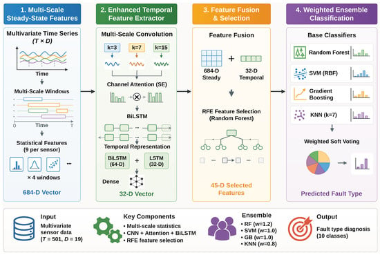
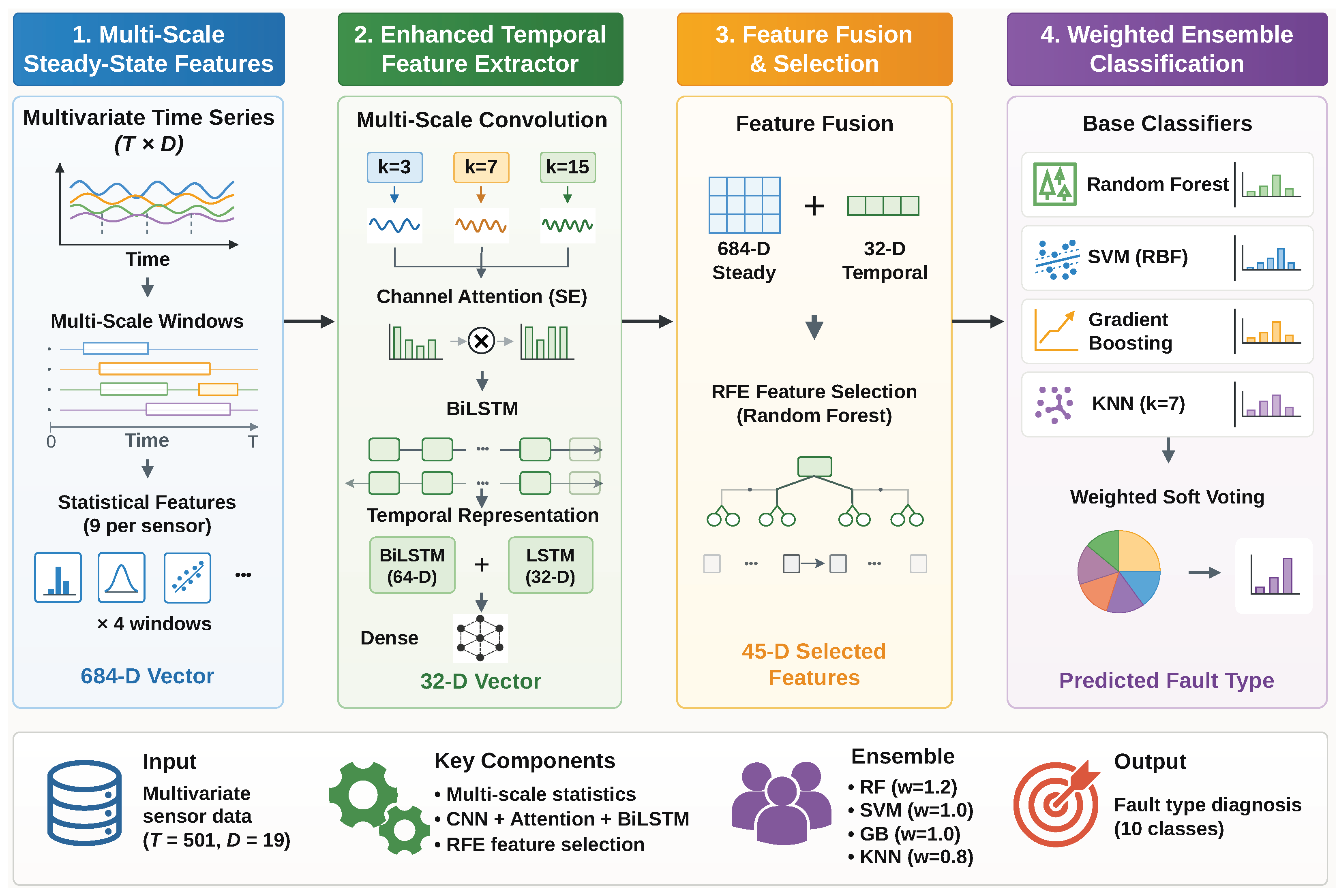
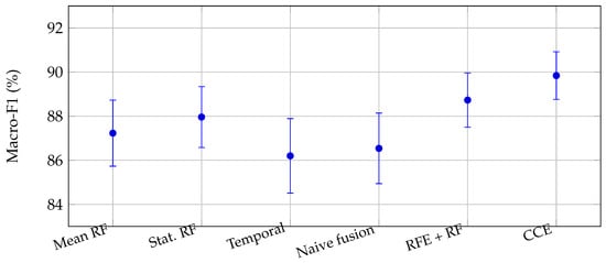
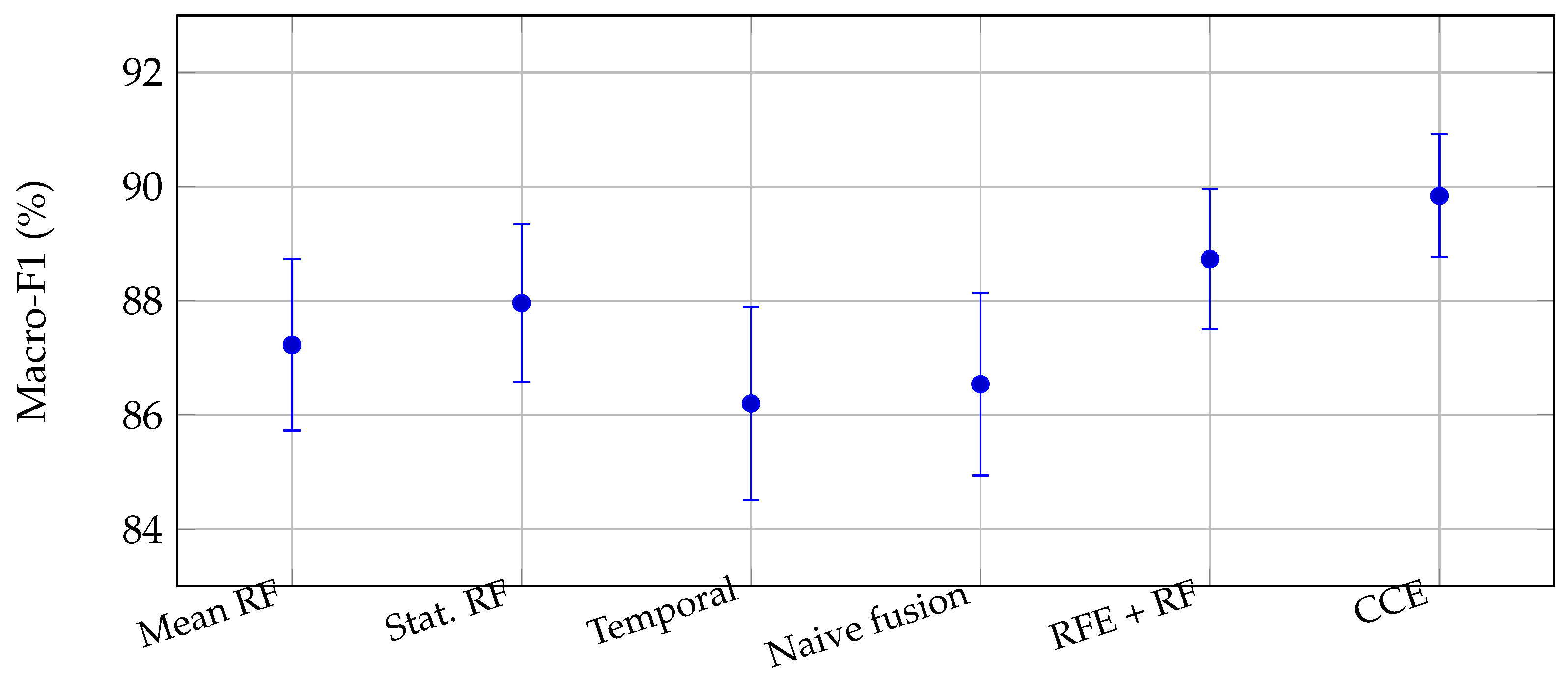
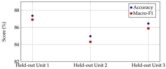
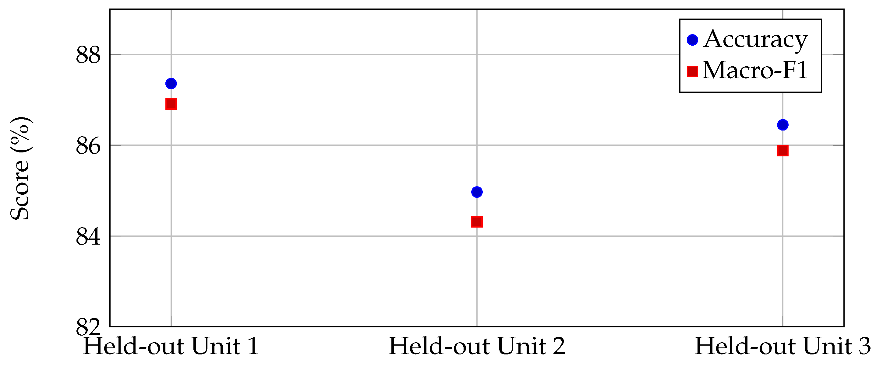

Disclaimer/Publisher’s Note: The statements, opinions and data contained in all publications are solely those of the individual author(s) and contributor(s) and not of MDPI and/or the editor(s). MDPI and/or the editor(s) disclaim responsibility for any injury to people or property resulting from any ideas, methods, instructions or products referred to in the content. |
© 2026 by the authors. Licensee MDPI, Basel, Switzerland. This article is an open access article distributed under the terms and conditions of the Creative Commons Attribution (CC BY) license.