Research on the Nonlinear Dynamic Theoretical Modeling and Response Characteristics of a Projectile–Fuze System Penetrating a Finite-Thickness Concrete Target

Featured Application

The theoretical modeling approach proposed in this paper offers effective guidance for the analysis of penetrating projectile–fuze systems.

Abstract

The dynamic behavior of projectile–fuze systems under high-velocity penetration is extremely complex, which causes great challenges in fuze performance evaluation and design. Existing research mainly relies on numerical simulation, while the corresponding theoretical studies are very limited. To overcome the limitations in current theoretical studies and provide a reliable reference model, this paper develops a nonlinear dynamic model for projectile–fuze systems penetrating finite-thickness concrete targets. The model adopts a hierarchical modeling strategy and comprehensively considers the projectile–target interaction, projectile–charge coupling effect, fuze system and projectile–fuze coupling. Based on the three-stage projectile–target penetration mechanism (cratering, tunneling, shear plugging), finite element (FE) dynamic theory, and the multi-degree-of-freedom (MDOF) lumped parameter approach, an integrated dynamic theoretical framework is established. On this basis, the influences of striking velocity, thickness and compressive strength of concrete target, and friction between the projectile and target on the dynamic characteristics of the projectile–fuze system are analyzed. The results suggest that in the process of penetration, the fuze overload response shows severe oscillations, which are mainly concentrated in the cratering stage and the early stage of tunneling. In this period, the striking velocity, target strength and friction have a significant impact on the overload response. Penetration velocity and resistance are highly dependent on the striking velocity, target strength, target thickness and the friction between the projectile and the target, and these factors affect the fuze overload response by influencing the penetration resistance and the projectile–target interaction time. The theoretical modeling method of the penetrating projectile–fuze system can serve as a guidance in related fields.

1. Introduction

As defensive systems develops, important military targets are increasingly protected by complex reinforced structures, which renders hard-target penetration weapons an important means to destroy such targets. Penetration fuze is the core control system of penetration weapons, and its performance directly determines whether the weapon can accurately identify the target and achieve precise damage control [1,2]. However, under the conditions of high-velocity impact and complex target, the internal load environment of the fuze is extremely harsh and complex, posing severe challenges to its survivability and reliability.

The dynamic behavior of projectile–fuze systems under high-velocity penetration is extremely complex, which causes great challenges in fuze performance evaluation and design. At present, finite element simulation is the primary means of investigating penetration fuzes. However, theoretical studies on the dynamic response of penetration fuzes are rather limited, particularly for integrated theoretical modeling covering the full projectile–charge–fuze–target chain. Although numerical simulation can obtain the overload response of fuzes, the results highly rely on the mesh quality and material model. Meanwhile, the underlying mechanical mechanisms of fuze overload transmission cannot be uncovered. Therefore, it is necessary to investigate the dynamic characteristics of penetration fuzes from a theoretical perspective, so as to provide theoretical support for the engineering design of high-velocity penetration fuzes.

The dynamic characteristics of penetration fuzes are determined by the process of projectile penetration into targets. Accordingly, research on penetration fuzes cannot be carried out independently and must be based on the investigation of projectile penetration. Over the past few decades, scholars have conducted extensive and in-depth research on the issue of projectile penetration [3]. In particular, the dynamic cavity expansion theory originally established and developed by Bishop [4], Hopkins [5] and Forrestal [6] has laid a theoretical foundation for projectile penetration research and enables theoretical analysis for various complex penetration problems [7,8,9]. Based on this theory, researchers have conducted substantial theoretical studies on the penetration resistance [10,11], penetration depth [12,13,14], residual velocity [15], cratering characteristics of targets [16,17,18], and trajectory [19]. For example, Yankelevsky [10] challenged the traditional conclusion that penetration depth is inversely proportional to the square root of concrete unconfined compressive strength and verified that concrete with identical unconfined compressive strength shows different penetration resistance. Zhang et al. [13] proposed an improved spherical cavity expansion theory based on the Tresca yield criterion and established a prediction method for penetration depth of rigid projectiles with different head shapes. Chen et al. [16,17] divided the process of the projectile penetrating the concrete into three stages: initial cratering, tunneling and shear plugging. Duan et al. [18] deeply analyzed the penetration mechanism under different target thicknesses and divided finite-thickness concrete targets into thin, medium and thick targets. Meanwhile, based on the three-stage model, they also developed corresponding theoretical frameworks for these three types of targets to predict the attitude angle of projectile during oblique penetration. Li et al. [19] proposed a trajectory model for the projectile oblique penetrating into the concrete targets.

Although the aforementioned studies have achieved remarkable success in describing the physical processes of projectile penetration, most of them focus on macroscopic terminal effects under the rigid-body assumption. The overload obtained from such models only reflects the overall response characteristics of the projectile and cannot serve as a reliable basis for evaluating the loading environment of the fuze. A large number of experiments have shown that during the process of the projectile penetrating the target at high velocity, the overload signals sensed by the fuze are more complex, manifested as the superposition of a large number of high-frequency and high-amplitude oscillation signals [20,21]. The main reasons leading to this phenomenon include the following two aspects [21,22,23,24,25,26]. On one hand, the projectile is not a rigid body. During high-velocity impact condition, stress waves will propagate and superimpose. On the other hand, the projectile–fuze structure actually is an MDOF system. The nonlinearity of the connection interface, as well as the internal structure composition and mass distribution of the fuze, result in the overload signals perceived by the fuze sensor containing a large amount of noise and structural interference. Therefore, the dynamic response characteristics of the penetration projectile–fuze system and the actual overload of the fuze are difficult to evaluate and predict.

FE simulation can characterize strong nonlinear dynamic behaviors including structural deformation, high strain rate effects, material failure and contact between components during penetration [27,28], which has become the primary method for investigating penetration fuzes. Researchers have conducted extensive studies on projectile–fuze systems using simulation software, and it has become an indispensable tool in this field. In particular, the explicit FE solver LS-DYNA exhibits unique advantages in solving large deformation and high strain rate impact problems, and has been widely applied to penetration dynamic simulations [29,30]. Classic constitutive models such as Holmquist–Johnson–Cook (HJC) [31] and Riedel–Hiermaier–Thoma (RHT) [32] have laid a theoretical foundation for this type of numerical simulation. In contrast, theoretical dynamic modeling studies for penetration projectile–fuze systems are extremely limited. Some scholars have already noticed this issue and have made some attempts in theory. For example, Cheng et al. [33] introduced the vibration theory into the study of the dynamic response of the penetration projectile system. They assumed the vibration of the projectile as the linear superposition of various axial vibrations and proposed a simplified dynamic model of the penetration projectile–fuze system. However, stress wave propagation inside the projectile, internal structural vibration of the fuze and the influence of charge were not considered. Yu et al. [34] established a multibody system dynamics model for penetration projectile–fuze systems. Meanwhile, they also studied the transmission law of impact loads between the projectile and the fuze. Although they considered the load transmission within the fuze structure and established an MDOF dynamic model for the fuze system, the projectile was simplified as a lumped mass and coupled with the fuze system only via stiffness and damping elements. Meanwhile, their model fails to account for the propagation of impact response inside the projectile and ignores the dynamic effect of charges, which introduces inherent limitations to the theoretical model. In addition, there are problems with the method of determining the stiffness and damping of the fuze structure through FE harmonic response analysis. Zheng et al. [35] established a nonlinear dynamic model of the projectile–fuze system under high-velocity penetration conditions. They comprehensively considered the projectile–target interaction and the propagation effect of stress waves within the projectile, while incorporating the load transfer characteristics of threaded connections and the nonlinear response behavior of buffer materials. However, they overly simplified the fuze structure and neglected the coupling effect between the projectile and charge, which fails to account for the charge influence and the interactions among internal fuze components.

Overall, although researchers have extensively investigated the dynamic behavior of the projectile and fuze under high-velocity penetration impact, an integrated theoretical modeling method for projectile–fuze systems that couples the projectile, charge, fuze and target is still lacking. Therefore, it is necessary to establish a theoretical model that can reasonably characterize the dynamic response mechanism of a projectile–fuze system during high-velocity penetration, so as to provide theoretical support for the structural design and optimization of penetration fuzes. To address the above issue, this paper develops a coupled dynamic model for the full response chain spanning from projectile–target interaction to internal fuze dynamic response based on classical penetration theory, FE theory and elastic mechanics theory. By incorporating projectile–target interaction, projectile–charge coupling, fuze structural characteristics, and projectile–fuze coupling, an integrated theoretical modeling method for the projectile–charge–fuze–target system is established, which can provide relatively complete theoretical support for the design of penetration fuzes.

2. Structure and Load Transmission Characteristics of the Projectile–Fuze System

Under high-velocity penetration, the fuze acquires penetration overload signals in real time using a built-in accelerometer, and its initiation control module conducts initiation control based on the real-time overload signals for precise damage. During high-velocity penetration process, the projectile nose is subjected to extreme impact loads, which are transmitted through multiple layers of structures such as the projectile, charge, and fuze base to the internal components of the fuze and finally sensed by the acceleration sensor. Due to the complexity of the projectile–fuze system, the overload signals sensed by the acceleration sensor contain structural and environmental interference, thus generating a large number of high-frequency components. Figure 1 shows a typical projectile–fuze structure, mainly consisting of the projectile, charge, projectile–fuze connection, detonation sequence, fuze and its internal components. The projectile is usually made of high-strength alloy metal materials. The penetration fuze is generally engaged into the fuze base through the threaded connection structure. The fuze mainly consists of the initiation control module, acceleration sensor, detonation sequence, buffering and potting structure. The buffering structure is used to reduce the intense impact loads transmitted to the fuze during high-velocity penetration, preventing structural failure and signal distortion. The potting structure achieves component fixation and electrical insulation protection. Meanwhile, it can dissipate impact stress in coordination with the buffer structure to enhance the shock resistance of the fuze under high-overload environments.

Figure 1. Structure of projectile–fuze system.

3. Nonlinear Dynamic Theoretical Modeling for the Projectile–Fuze System

3.1. Fundamental Assumptions

The dynamic modeling of a projectile–fuze system penetration is highly complex, and several assumptions must be introduced. The fundamental assumptions adopted in this paper are listed as follows:

(1)

Mass loss of the projectile is neglected. This assumption is widely adopted in penetration research and holds when the interfacial pressure on the projectile during penetration is insufficient to cause notable plastic flow and mass loss [11,16,17,36,37].

(2)

The projectile does not undergo plastic deformation during the penetration process. The kinetic energy of the projectile is expended to overcome the resistance of projectile–target interaction.

(3)

The deflection of projectile attitude is not considered, and the projectile maintains a normal impact state.

(4)

Concrete is preictally an anisotropic, inhomogeneous material. The mechanical performance of concrete is highly influenced by the configuration of steel rebars and aggregates. This paper does not focus on concrete material behavior itself, the effects of rebars and aggregates are neglected to simplify the analysis, and the concrete is considered plain concrete without reinforcement.

(5)

For the analysis of projectile–target interaction, the rigid-body assumption for the projectile is accepted, which is widely used in projectile penetration research [15,17,36]. Nevertheless, structural deformations of the projectile and charge are taken into account within the elastic regime in their structural modeling.

(6)

Interfacial contact effects among various components of the projectile–fuze system are neglected. Accordingly, the dominant source of nonlinearity arises from the nonlinear characteristic of the projectile–target interaction resistance.

(7)

Only mechanical effects of penetration are considered, while impact-induced thermal effects, heat transfer and temperature fields are neglected.

3.2. Projectile–Target Interaction

Research on projectile penetration is mostly based on Forrestal’s model [36], which divides the penetration process into the initial cratering stage and tunneling stage. However, this model is applicable only to semi-infinite concrete targets. When a projectile penetrates a finite-thickness concrete target, perforation usually occurs instead of the projectile being trapped inside the target. Different from the case of thin targets, the projectile can experience a complete cratering stage. Moreover, if the target thickness is relatively large or the initial striking velocity is low, the projectile may eventually be stopped inside the target after completing the cratering and tunneling stages. For generality, a more completed theoretical model will be developed to describe the physical process of projectile penetration and perforation into finite-thickness concrete targets.

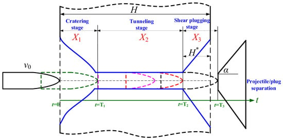
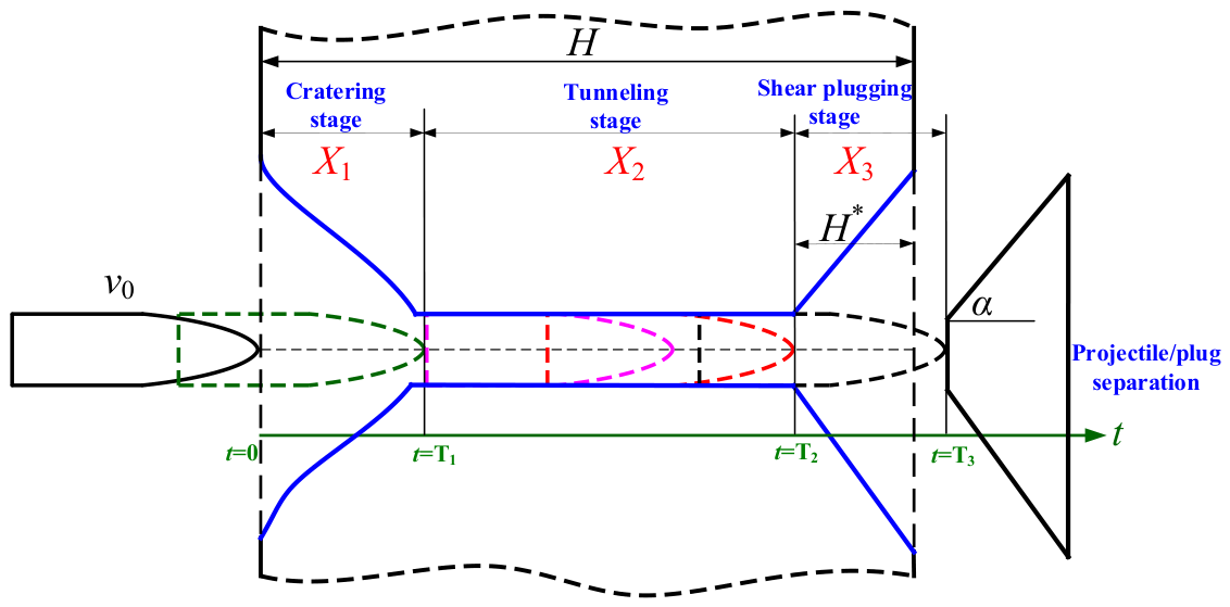
Consider a projectile that normally penetrates a finite-thickness concrete target. According to the assumptions proposed by Chen et al. [16,17], the projectile will undergo three complete stages, i.e., cratering stage, tunneling stage and shear plugging stage. The complete penetration process is shown in Figure 2.

Figure 2. A schematic diagram of the projectile penetrating a finite-thickness concrete target.

The projectile decelerates under the resistance caused by concrete. According to Newton’s second law, a unified motion equation can be formulated to describe the motion of the projectile in all three penetration stages:

$$m{\displaystyle \frac{d^2{x}_i\left(t\right)}{d{t}^2}}=-F_{ni}\left(i=1,2,3\right)$$

(1)

where $i=1,2,3$ denotes the cratering, tunneling, and shear plugging stages, respectively. $F_{ni}$ represents the axial resistance acting on the projectile during the projectile–target interaction.

According to Refs. [16,17,18,36], the axial resistance acting on the projectile can be expressed as

$$\left\{\begin{array}{l}{F}_{n1}=c_1{x}_1\left(t\right)\\ F_{n2}={\displaystyle \frac{1}{4}}\pi d^2\left(R{N}_1+{\rho }_{0}B{v}^2{N}_2\right)\\ F_{n3}=c_2{x}_3\left(t\right)-F_{ns}=c_2{x}_3\left(t\right)-{\displaystyle \frac{1}{\sqrt{3}}}{f}_c\pi d{H}^{*}\left(1+{\displaystyle \frac{H^{*}}{d}}\tan \alpha \right)\end{array}\right.,$$

(2)

where $c_1$ and $c_2$ are the parameters related to the target and $d$ is the projectile diameter. $B$ is a dimensionless parameter determined by the concrete material [33]. ${\rho }_0$ is the density of concrete. $N_1$ and $N_2$ are nose shape coefficients. $H^{*}$ and $\alpha$ represent the thickness and cone angle of the plug, respectively. R represents the static resistance term of concrete, which can be determined by $R=S{f}_c$, where $S$ is a dimensionless constant and $f_c$ is the unconfined compress strength. At present, many studies take $S=72.0f_c^{-0.5}$ or $S=82.6f_c^{-0.544}$ [16,17], but scholars have found that the value of $S$ is affected by the size effect of the projectile [38]. If the value of $S$ obtained under small-scale conditions is adopted for calculations of large-scale cases, the penetration resistance will be overestimated. According to experimental data fitting, Wu et al. [38] suggested that $S=25.83d^{-0.254}{f}_c^{-0.5}$, where the unit of $d$ and $f_c$ is m and MPa, respectively.

3.2.1. Cratering Stage

We assume that the initial penetration velocity of the projectile is $v_0$. Hence, based on Equation (1) and the initial conditions, the penetration depth, velocity, and acceleration of the projectile during the cratering stage can be obtained as follows:

$$\left\{\begin{array}{l}{x}_1\left(t\right)={\displaystyle \frac{v_0}{\sqrt{c_1/m}}}\sin \sqrt{{\displaystyle \frac{c_1}{m}}}t\\ v_1\left(t\right)={\displaystyle \frac{d{x}_1\left(t\right)}{dt}}=v_0\cos \sqrt{{\displaystyle \frac{c_1}{m}}}t\\ a_1\left(t\right)={\displaystyle \frac{d{v}_1\left(t\right)}{dt}}=-v_0\sqrt{{\displaystyle \frac{c_1}{m}}}\sin \sqrt{{\displaystyle \frac{c_1}{m}}}t\end{array}\right.$$

(3)

where m is the mass of the projectile. Meanwhile, at the end of the cratering stage, $t=T_1$ (i.e., the start of the tunneling stage), the trajectory distance is $X_1=x_1\left(T_1\right)$, the velocity of the projectile is $V_1=v_1\left(T_1\right)$, and the acceleration of the projectile is $A_1=a_1\left(T_1\right)$. Then, we can obtain the following:

$$\left\{\begin{array}{l}{X}_1\left(t\right)=kd={\displaystyle \frac{v_0}{\sqrt{c_1/m}}}\sin \sqrt{{\displaystyle \frac{c_1}{m}}}{T}_1;\\ V_1\left(t\right)=v_0\cos \sqrt{{\displaystyle \frac{c_1}{m}}}{T}_1;\\ A_1\left(t\right)=-v_0\sqrt{{\displaystyle \frac{c_1}{m}}}\sin \sqrt{{\displaystyle \frac{c_1}{m}}}{T}_1\end{array}\right.$$

(4)

where $k$ denotes the resistance coefficient of the crating stage, which can take the value of $k=2$ recommended in [36] or $k=0.707+h/d$ given in [16,17].

Moreover, at the end of the cratering stage, the axial resistance satisfies the following relation:

$$\left\{\begin{array}{l}{X}_1=kd\\ F_{n1}=c_1{X}_1=F_{n2}={\displaystyle \frac{1}{4}}\pi d^2\left(R{N}_1+{\rho }_{0}B{v}^2{N}_2\right)\end{array}\right.$$

(5)

Therefore, substituting Equation (5) into Equation (4) yields the following:

$$\left\{\begin{array}{l}{V}_1^2={\displaystyle \frac{m{v}_0^2-\left(\pi k{d}^3/4\right)R{N}_1}{m+\left(\pi k{d}^3/4\right){\rho }_{0}B{N}_2}}\\ c_1={\displaystyle \frac{\pi d}{4k}}\left({\displaystyle \frac{R{N}_1+v_0^2{\rho }_{0}B{N}_2}{1+\left(\pi k{d}^3/4m\right){\rho }_{0}B{N}_2}}\right)\\ T_1=\sqrt{{\displaystyle \frac{m}{c_1}}}\arccos \left({\displaystyle \frac{V_1}{v_0}}\right)\end{array}\right.$$

(6)

3.2.2. Tunneling Stage

At the tunneling stage, the projectile nose fully penetrates into the target and the lateral resistance acted on the projectile is symmetric. Hence, the projectile moves forward in a straight line under axial resistance, i.e., $F_{n2}=\pi d^2/4\left(R{N}_1+{\rho }_{0}B{v}^2{N}_2\right)$ [36]. It should be noted that when the penetration velocity of the projectile decreases to a value insufficient to perforate the concrete target, the projectile will come to rest into the target, with both its velocity and acceleration dropping to zero. In this case, the projectile only experiences the complete cratering and tunneling stages. Therefore, in practical calculation, the penetration depth should be calculated to determine whether the projectile enters the shear plugging stage.

Integrating the motion equation of the projectile $m{d}^2{x}_2\left(t\right)/d{t}^2=-\pi d^2/4\left(R{N}_1+{\rho }_{0}B{v}_2^2{N}_2\right)$ from $V_1$ to zero and $kd$ to $P$ gives the penetration depth:

$$P={\displaystyle \frac{2m}{\pi d^2{\rho }_{0}B{N}_2}}\ln \left(1+{\displaystyle \frac{{\rho }_{0}B{N}_2{V}_1^2}{R{N}_1}}\right)+kd$$

(7)

The velocity of the projectile during the tunneling stage can be obtained by

$$v_2\left(t\right)=\sqrt{{\displaystyle \frac{R{N}_1}{B{\rho }_0{N}_2}}}\tan \left\{\arctan \left(v_1\sqrt{{\displaystyle \frac{B{\rho }_0{N}_2}{R{N}_1}}}\right)-\sqrt{N_1{N}_{2}B{\rho }_{0}R}{\displaystyle \frac{\pi d^2}{4m}}\left(t-T_1\right)\right\}.$$

(8)

Taking the derivative of the velocity with respect to time, the acceleration of projectile can be obtained as follows:

$$a_2\left(t\right)={\displaystyle \frac{d{v}_2\left(t\right)}{dt}}={\displaystyle \frac{-\frac{\pi d^{2}R{N}_1}{4m}}{{\cos }^2\left\{\arctan \left(V_1\sqrt{\frac{B{\rho }_0{N}_2}{R{N}_1}}\right)-\sqrt{N_1{N}_{2}B{\rho }_{0}R}\frac{\pi d^2}{4m}\left(t-T_1\right)\right\}}}$$

(9)

3.2.3. Shear Plugging Stage

Shearing plugging is a typical failure mode of concrete targets verified by numerous penetration experiments. When a projectile penetrates a finite-thickness concrete target, a cavity with approximately conical contour will be formed on the rear of the target due to the plugging effect [39]. In the shear plugging stage, severe shear deformation occurs in the target material ahead of and around of the projectile nose, which gradually forms a plug separated from the target. Once the shear resistance is overcome, the plug is sheared off along the cone and detaches from the target. Finally, due to the velocity difference and rear-surface unloading, the plug separates from the projectile instantaneously upon exiting the target. In this stage, the axial resistance on the projectile can be approximately assumed to decrease linearly to zero [18]. Therefore, the motion equation of the projectile is $m{d}^2{x}_3\left(t\right)/d{t}^2=c_2{x}_3\left(t\right)-F_{ns}$. By solving this equation, the trajectory distance, velocity and acceleration of the projectile can be derived as follows:

$$\left\{\begin{array}{l}{x}_3\left(t\right)=\left(V_2\sqrt{{\displaystyle \frac{m}{4c_2}}}-{\displaystyle \frac{F_{ns}}{2c_2}}\right)\exp \left[\left(t-T_2\right)\sqrt{{\displaystyle \frac{c_2}{m}}}\right]-\left(V_2\sqrt{{\displaystyle \frac{m}{4c_2}}}+{\displaystyle \frac{F_{ns}}{2c_2}}\right)\exp \left[-\left(t-T_2\right)\sqrt{{\displaystyle \frac{c_2}{m}}}\right]+{\displaystyle \frac{F_{ns}}{c_2}}\\ v_3\left(t\right)=\sqrt{{\displaystyle \frac{c_2}{m}}}\left[\left(V_2\sqrt{{\displaystyle \frac{m}{4c_2}}}-{\displaystyle \frac{F_{ns}}{2c_2}}\right)\exp \left[\left(t-T_2\right)\sqrt{{\displaystyle \frac{c_2}{m}}}\right]-\left(V_2\sqrt{{\displaystyle \frac{m}{4c_2}}}+{\displaystyle \frac{F_{ns}}{2c_2}}\right)\exp \left[-\left(t-T_2\right)\sqrt{{\displaystyle \frac{c_2}{m}}}\right]\right]\\ a_3\left(t\right)={\displaystyle \frac{c_2}{m}}\left[\left(V_2\sqrt{{\displaystyle \frac{m}{4c_2}}}-{\displaystyle \frac{F_{ns}}{2c_2}}\right)\exp \left[\left(t-T_2\right)\sqrt{{\displaystyle \frac{c_2}{m}}}\right]-\left(V_2\sqrt{{\displaystyle \frac{m}{4c_2}}}+{\displaystyle \frac{F_{ns}}{2c_2}}\right)\exp \left[-\left(t-T_2\right)\sqrt{{\displaystyle \frac{c_2}{m}}}\right]\right]\end{array}\right.$$

(10)

where $T_2$ and $V_2$ represent the time and velocity at the start of the shear plugging stage (i.e., the end of the tunneling stage). Assuming that the time, trajectory distance, velocity and acceleration at the end of the shear plugging stage are $t=T_3$, $X_3=x_3\left(T_3\right)$, $V_3=v_3\left(T_3\right)$, and $A_3=a_3\left(T_3\right)$, respectively, then we can obtain the following:

$$\left\{\begin{array}{l}{X}_3=\left(V_2\sqrt{{\displaystyle \frac{m}{4c_2}}}-{\displaystyle \frac{F_{ns}}{2c_2}}\right)\exp \left[\left(T_3-T_2\right)\sqrt{{\displaystyle \frac{c_2}{m}}}\right]-\left(V_2\sqrt{{\displaystyle \frac{m}{4c_2}}}+{\displaystyle \frac{F_{ns}}{2c_2}}\right)\exp \left[-\left(T_3-T_2\right)\sqrt{{\displaystyle \frac{c_2}{m}}}\right]+{\displaystyle \frac{F_{ns}}{c_2}}\\ V_3=\sqrt{{\displaystyle \frac{c_2}{m}}}\left[\left(V_2\sqrt{{\displaystyle \frac{m}{4c_2}}}-{\displaystyle \frac{F_{ns}}{2c_2}}\right)\exp \left[\left(T_3-T_2\right)\sqrt{{\displaystyle \frac{c_2}{m}}}\right]-\left(V_2\sqrt{{\displaystyle \frac{m}{4c_2}}}+{\displaystyle \frac{F_{ns}}{2c_2}}\right)\exp \left[-\left(T_3-T_2\right)\sqrt{{\displaystyle \frac{c_2}{m}}}\right]\right]\\ A_3={\displaystyle \frac{c_2}{m}}\left[\left(V_2\sqrt{{\displaystyle \frac{m}{4c_2}}}-{\displaystyle \frac{F_{ns}}{2c_2}}\right)\exp \left[\left(T_3-T_2\right)\sqrt{{\displaystyle \frac{c_2}{m}}}\right]-\left(V_2\sqrt{{\displaystyle \frac{m}{4c_2}}}+{\displaystyle \frac{F_{ns}}{2c_2}}\right)\exp \left[-\left(T_3-T_2\right)\sqrt{{\displaystyle \frac{c_2}{m}}}\right]\right]=0\end{array}\right.$$

(11)

3.2.4. Penetration Resistance of the Projectile

The above sections present the modeling process of the projectile penetrating the concrete target in three stages. Before deriving the penetration resistance for each stage, the continuity conditions for the three stages must be obtained. It is noted that the physical quantities at the end of the cratering stage are exactly those at the start of the tunneling stage. Similarly, the physical quantities at the end of the tunneling stage are those at the start of the shear plugging stage.

As shown in Equation (6), the physical quantities at the end of the cratering stage are known, while the time $T_2$, trajectory distance $X_2$, and projectile velocity $V_2$ at the end of the tunneling stage remain unknown. By integrating Equation (1), we can obtain

$$X_2={\displaystyle \frac{2m}{\pi d^2{\rho }_{0}B{N}_2}}\ln \left({\displaystyle \frac{R{N}_1+{\rho }_{0}B{N}_2{V}_1^2}{R{N}_1+{\rho }_{0}B{N}_2{V}_2^2}}\right).$$

(12)

From Figure 2, it can be seen that the trajectory distance of the projectile in the tunneling and shear plugging stages satisfies the following:

$$\left\{\begin{array}{l}{X}_2=H-H^{*}-X_1\\ X_3=H^{*}\end{array}\right.$$

(13)

Meanwhile, at the instant when the tunneling stage ends and shear plugging begins, the axial resistance of the projectile satisfies $F_{n2}=F_{n3}$. Then, combining this with the above equation yields

$$\left\{\begin{array}{l}{H}^{\ast }=H-X_1-{\displaystyle \frac{2m}{\pi d^2{\rho }_{0}B{N}_2}}\ln \left({\displaystyle \frac{R{N}_1+{\rho }_{0}B{N}_2{V}_1^2}{R{N}_1+{\rho }_{0}B{N}_2{V}_2^2}}\right)\\ V_2^2={\displaystyle \frac{1}{{\rho }_{0}B{N}_2}}\left[{\displaystyle \frac{4}{\sqrt{3}d}}{f}_c{H}^{\ast }\left(1+{\displaystyle \frac{H^{\ast }}{d}}\tan \alpha \right)-R{N}_1\right]\end{array}\right..$$

(14)

The above equation is a system of nonlinear equations for $H^{\ast }$ and $V_2$, which can be solved using the Newton–Raphson iteration method. $T_2$ can be obtained by integrating Equation (1).

$$T_2={\displaystyle \frac{4m}{\pi d^2\sqrt{N_1{N}_{2}B{\rho }_{0}R}}}\left[\arctan \left(V_1\sqrt{{\displaystyle \frac{B{\rho }_0{N}_2}{R{N}_1}}}\right)-\arctan \left(V_2\sqrt{{\displaystyle \frac{B{\rho }_0{N}_2}{R{N}_1}}}\right)\right]+T_1$$

(15)

Furthermore, $c_2$ and $T_3$ can be obtained as follows:

$$\left\{\begin{array}{l}{c}_2={\displaystyle \frac{F_{ns}}{X_3}}={\displaystyle \frac{1}{\sqrt{3}}}{f}_c\pi d{H}^{*}\left(1+{\displaystyle \frac{H^{*}}{d}}\tan \alpha \right)\\ T_3=T_2-\sqrt{{\displaystyle \frac{c_2}{4m}}}\left\{\ln \left(V_2\sqrt{{\displaystyle \frac{m}{4c_2}}}-{\displaystyle \frac{F_{ns}}{2c_2}}\right)-\ln \left(V_2\sqrt{{\displaystyle \frac{m}{4c_2}}}+{\displaystyle \frac{F_{ns}}{2c_2}}\right)\right\}\end{array}\right.$$

(16)

Based on the above analysis, the axial resistance of the projectile penetrating a finite-thickness concrete target can be uniformly expressed as follows:

The projectile only experiences the cratering and tunneling stages:

$$F\left(t\right)=\left\{\begin{array}{l}-m{v}_0\sqrt{{\displaystyle \frac{c_1}{m}}}\sin \left(\sqrt{{\displaystyle \frac{c_1}{m}}}t\right)\hspace{1em}\hspace{1em}\hspace{1em}t\in \left[0,T_1\right];x\left(t\right)\in \left[0,X_1\right]\\ {\displaystyle \frac{-\pi d^{2}R{N}_1}{4 {\cos }^2\left\{\arctan \left(V_1\sqrt{\frac{B{\rho }_0{N}_2}{R{N}_1}}\right)-\sqrt{N_1{N}_{2}B{\rho }_{0}R}\frac{\pi d^2}{4m}\left(t-T_1\right)\right\}}}\hspace{1em}\hspace{1em}t\in \left[T_1,T_2\right];x\left(t\right)\in \left[X_1,P\right]\end{array}\right.$$

(17)

The projectile experiences all three stages:

$$F\left(t\right)=\left\{\begin{array}{l}-m{v}_0\sqrt{{\displaystyle \frac{c_1}{m}}}\sin \left(\sqrt{{\displaystyle \frac{c_1}{m}}}t\right)\hspace{1em}\hspace{1em}\hspace{1em}\hspace{1em}t\in \left[0,T_1\right];x\left(t\right)\in \left[0,X_1\right]\\ {\displaystyle \frac{-\pi d^{2}R{N}_1}{4 {\cos }^2\left\{\arctan \left(V_1\sqrt{\frac{B{\rho }_0{N}_2}{R{N}_1}}\right)-\sqrt{N_1{N}_{2}B{\rho }_{0}R}\frac{\pi d^2}{4m}\left(t-T_1\right)\right\}}}\hspace{1em}\hspace{1em}t\in \left[T_1,T_2\right];x\left(t\right)\in \left[X_1,X_2\right]\\ c_2\left[\left(V_2\sqrt{{\displaystyle \frac{m}{4c_2}}}-{\displaystyle \frac{F_{ns}}{2c_2}}\right)e^{\left(t-T_2\right)\sqrt{{\displaystyle \frac{c_2}{m}}}}-\left(V_2\sqrt{{\displaystyle \frac{m}{4c_2}}}+{\displaystyle \frac{F_{ns}}{2c_2}}\right)e^{-\left(t-T_2\right)\sqrt{{\displaystyle \frac{c_2}{m}}}}\right]\hspace{1em}\hspace{1em}t\in \left[T_2,T_3\right];x\left(t\right)\in \left[X_2,X_3\right]\end{array}\right.$$

(18)

3.3. Coupled Dynamic Equations for the Projectile–Charge Structure

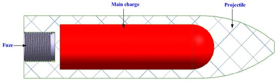
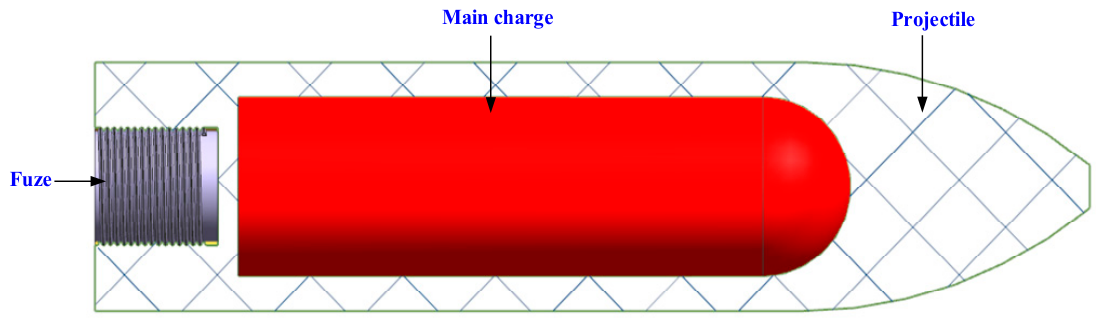
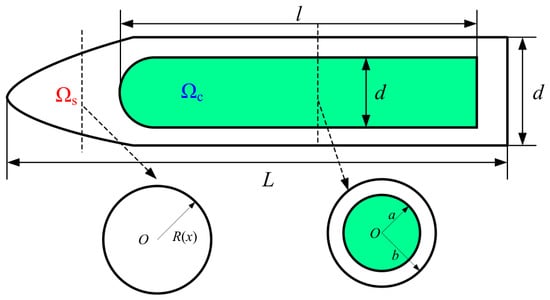
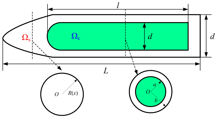
During high-velocity penetration, stress waves are generated inside the projectile. The waves propagate through the projectile at the longitudinal wave speed and reflect at projectile ends. As the charge occupies most of the warhead volume, stress wave propagation is inevitably influenced by it. In practice, mechanical coupling occurs between the projectile body and charge. Accordingly, they are regarded as an integrated coupled structure in this section. The coupling relationship is formulated via the elastic thick-walled cylinder theory, and the projectile–charge coupled structure is mechanically equivalent to a composite structure. As shown in Figure 3, the penetration warhead consists of the projectile (${\mathrm{\Omega }}_s$) and charge (${\mathrm{\Omega }}_c$). The radii of projectile and charge are a and b, respectively.

Figure 3. Structure of penetration warhead.

It is noted that the local regions of the projectile may experience high strain rates and localized yielding during penetration. However, such local plasticity is concentrated at the projectile tip and has limited influence on stress wave propagation and overload transmission within the projectile. Hence, the projectile is assumed to be linear elastic in this subsection. In addition, the projectile and the charge are perfectly bonded together, with them in close contact. Relative sliding is ignored.

According to the above hypothesis, the projectile and charge can be analyzed using elastic theory. The axial displacements of the projectile and charge are assumed to be the same, $u\left(x,t\right)$, and so are the axial strains, ${\epsilon }_x=\partial u/\partial x$. Meanwhile, the projectile and charge satisfy the continuity condition at the radial interface, i.e., ${\left.w_s\left(r,x,t\right)\right|}_{r=a}={\left.w_c\left(r,x,t\right)\right|}_{r=a}$. Under high-velocity impact conditions, due to the different Poisson’s ratios of the projectile and charge (${\mu }_s\ne {\mu }_c$), they will undergo different radial deformations and generate radial interface stress. The interface pressure is assumed to be p. Therefore, to treat the projectile and charge as a coupled and equivalent composite structure, the relevant mechanical parameters must be corrected.

3.3.1. Mechanical Parameters of Projectile–Charge Coupling Structure

We assume that the projectile and charge are isotropic circular bars subjected to uniformly distributed external pressure and axial stress. Then, their radial stress equilibrium equation is

$${\displaystyle \frac{d{\sigma }_{rk}}{dr}}+{\displaystyle \frac{{\sigma }_{rk}-{\sigma }_{\theta k}}{r}}=0,$$

(19)

where $k=s,c$ denotes the projectile and charge.

Taking the projectile as an example, according to the thick-walled cylinder theory, the general solution of the radial displacement of the above equation is

$$w_r^s\left(r\right)=C_{1}r+{\displaystyle \frac{C_2}{r}}.$$

(20)

So, the strain components can be obtained as

$${\epsilon }_r^s={\displaystyle \frac{d{w}_r^s}{dr}}=C_1-{\displaystyle \frac{C_2}{r^2}};{\epsilon }_{\theta }^s={\displaystyle \frac{w_r^s}{dr}}=C_1+{\displaystyle \frac{C_2}{r^2}};{\epsilon }_x^s=\epsilon .$$

(21)

The volumetric strain is $e={\epsilon }_r^s+{\epsilon }_{\theta }^s+{\epsilon }_x^s=2C_1+\epsilon$. Hence, the radial stress is

$${\sigma }_r^s={\lambda }_{s}e+2{\xi }_s{\epsilon }_r^s={\lambda }_s\left(2C_1+\epsilon \right)+2{\xi }_s\left(C_1-{\displaystyle \frac{C_2}{r^2}}\right),$$

(22)

where ${\lambda }_s$ and ${\xi }_s$ are Lame constants, ${\lambda }_s=E_s{\mu }_s/\left(1+{\mu }_s\right)\left(1-2{\mu }_s\right)$, and ${\xi }_s=E_s/2\left(1+{\mu }_s\right)$. The boundary condition is ${\left.{\sigma }_r^s\right|}_{r=a}=-p$, ${\left.{\sigma }_r^s\right|}_{r=b}=0$. Therefore, the coefficient in Equation (22) can be determined as $C_1={\displaystyle \frac{-{\lambda }_s\epsilon +\frac{p{a}^2}{b^2-a^2}}{2\left({\lambda }_s+{\xi }_s\right)}}$, $C_2={\displaystyle \frac{p}{2{\xi }_s}}{\displaystyle \frac{a^2{b}^2}{b^2-a^2}}$. Substituting $C_1$ and $C_2$ into Equation (20), the radial displacement of the projectile can be obtained as

$${\left.w_r^s\right|}_{r=a}=-{\displaystyle \frac{{\lambda }_{s}a}{2\left({\lambda }_s+{\xi }_s\right)}}\epsilon +{\displaystyle \frac{pa}{b^2-a^2}}\left[{\displaystyle \frac{a^2}{2\left({\lambda }_s+{\xi }_s\right)}}+{\displaystyle \frac{b^2}{2{\xi }_s}}\right].$$

(23)

Since ${\displaystyle \frac{{\lambda }_s}{{\lambda }_s+{\xi }_s}}=2{\mu }_s$, ${\displaystyle \frac{{\lambda }_s}{2\left({\lambda }_s+{\xi }_s\right)}}={\displaystyle \frac{\left(1+{\mu }_s\right)\left(1-2{\mu }_s\right)}{E_s}}$, ${\displaystyle \frac{1}{2{\xi }_s}}={\displaystyle \frac{1+{\mu }_s}{E_s}}$, then

$${\left.w_r^s\right|}_{r=a}=-a{\mu }_s\epsilon +pa\Gamma ,$$

(24)

where $\Gamma ={\displaystyle \frac{1+{\mu }_s}{E_s\left(b^2-a^2\right)}}\left[a^2\left(1-2{\mu }_s\right)+b^2\right]$.

Similarly, the radial displacement of the charge can be obtained as

$${\left.w_c^s\right|}_{r=a}=-a{\mu }_c\epsilon -{\displaystyle \frac{ap}{E_c}}\left(1+{\mu }_c\right)\left(1-2{\mu }_c\right).$$

(25)

Therefore, based on the continuity condition of the interface between the projectile and charge, ${\left.w_s\left(r,x,t\right)\right|}_{r=a}={\left.w_c\left(r,x,t\right)\right|}_{r=a}$, and it can be known that

$$p=K\epsilon ,K={\displaystyle \frac{{\mu }_s-{\mu }_c}{\Gamma +\frac{1}{E_c}\left(1-2{\mu }_c\right)\left(1+{\mu }_c\right)}}.$$

(26)

Hence, the axial stress of the projectile and charge can be determined by

$$\left\{\begin{array}{l}{\sigma }_x^s={\lambda }_{s}e+2{\xi }_s\epsilon =E_s\epsilon +2{\mu }_s{\displaystyle \frac{p{a}^2}{b^2-a^2}}\\ {\sigma }_x^c=E_c\epsilon -2{\mu }_{c}p=\left(E_c-2{\mu }_{c}K\right)\epsilon \end{array}\right..$$

(27)

Then, the axial load on the warhead at a certain position is

$$F={\sigma }_x^s{A}_s+{\sigma }_x^c{A}_c=\left[E_s{A}_s+E_c{A}_c+2K\left({\displaystyle \frac{{\mu }_s{a}^2{A}_s}{b^2-a^2}}\right)-{\mu }_c{A}_c\right]\epsilon =E_{eff}^{*}{A}_{eff}^{*}\epsilon .$$

(28)

According to Equation (28), the equivalent elastic parameters of the projectile–charge coupling structure can be expressed as $E_{eff}^{*}{A}_{eff}^{*}=E_s{A}_s+E_c{A}_c+2K\left({\displaystyle \frac{{\mu }_s{a}^2{A}_s}{b^2-a^2}}-{\mu }_c{A}_c\right)$.

3.3.2. Dynamic Control Equation for Projectile–Charge Structure

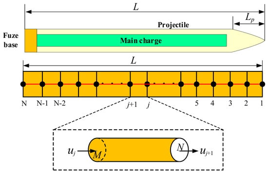
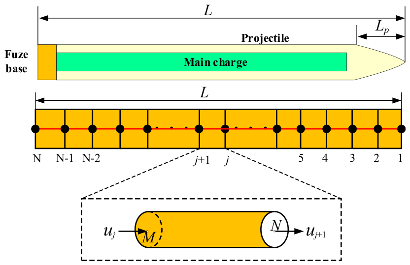
In this section, the dynamic equation of the projectile–charge coupling structure will be established by using FE theory. As shown in Figure 4, the projectile–charge structure is discretized into m elements along the axial direction, and the total number of nodes is N = m + 1. Meanwhile, only axial motion is considered, so each node has only one degree of freedom (DOF). It is assumed that the corresponding nodal displacement is $u_j\left(t\right)$, and each element can be represented by the element node vector ${\mathit{q}}_{ej}^T=\left(u_j,u_{j+1}\right)$. Then, the overall DOF of the projectile–charge structure can be expressed as

$${\mathit{u}}_b={\left(u_1,u_1,u_1,\cdots u_N\right)}^T.$$

(29)

Figure 4. Discretization of projectile–charge structure.

Assuming a polynomial displacement mode for the element, the displacement mode within the element can be described using the shape function $\mathit{N}=\left(N_1,N_2\right)$. The specific form of the shape function is

$$N_1=1-\xi ,N_2=\xi ,\xi ={\displaystyle \frac{x-x_i}{l_e}},$$

(30)

where $l_e$ is the length of the element. Hence, the axial displacement in the element is

$$u\left(x,t\right)=N_1{u}_j+N_2{u}_{j+1}=\mathit{N}{\mathit{q}}_{ej}^T.$$

(31)

The axial strain of the element is expressed as

$${\epsilon }_{ej}={\displaystyle \frac{\partial u}{\partial x}}={\displaystyle \frac{\partial \mathit{N}}{\partial x}}{\mathit{q}}_{ej}^T={\mathit{B}}_{ej}{\mathit{q}}_{ej}^T,$$

(32)

where ${\mathit{B}}_{ej}={\displaystyle \frac{\partial \mathit{N}}{\partial x}}={\displaystyle \frac{1}{l_e}}\left(-1,1\right)$.

Considering the lateral motion of the particle, the lateral displacement and velocity of the projectile and charge can be expressed as follows [40]:

$$\left\{\begin{array}{l}{w}_s\left(r,t\right)=-{\mu }_{s}r{\mathit{B}}_{ej}{\mathit{q}}_{ej}^T;{\dot{w}}_s\left(r,t\right)=-{\mu }_{s}r{\mathit{B}}_{ej}{\dot{\mathit{q}}}_{ej}^T\\ w_c\left(r,t\right)=-{\mu }_{c}r{\mathit{B}}_{ej}{\mathit{q}}_{ej}^T;{\dot{w}}_c\left(r,t\right)=-{\mu }_{c}r{\mathit{B}}_{ej}{\dot{\mathit{q}}}_{ej}^T\end{array}\right.$$

(33)

Accordingly, the kinetic energy of the projectile–charge coupled element includes the axial and lateral kinetic energies of the projectile and charge, that is,

$$\begin{array}{l}{T}^e={\displaystyle {\int }_0^{l_e}\frac{1}{2}\left({\rho }_s{A}_s+{\rho }_c{A}_c\right){\dot{u}}^2\left(x,t\right)+{\displaystyle {\int }_0^{l_e}\frac{1}{2}{\rho }_s{\displaystyle {\int }_a^b{\dot{w}}_s^2\left(r,t\right)2\pi rdrdx}}+{\displaystyle {\int }_0^{l_e}\frac{1}{2}{\rho }_c{\displaystyle {\int }_0^a{\dot{w}}_c^2\left(r,t\right)2\pi rdrdx}}}\\ ={\displaystyle \frac{1}{2}}\left({\rho }_s{A}_s+{\rho }_c{A}_c\right){\displaystyle {\int }_0^{l_e}{\dot{\mathit{q}}}_{ej}^T{\mathit{N}}^T\mathit{N}{\dot{\mathit{q}}}_{ej}dx}+{\rho }_s{\mu }_s^2{\displaystyle {\int }_0^{l_e}{\displaystyle {\int }_a^b{\dot{\mathit{q}}}_{ej}^T{\mathit{B}}_{ej}^T{\mathit{B}}_{ej}{\dot{\mathit{q}}}_{ej}\pi r^{3}drdx}}+{\rho }_c{\mu }_c^2{\displaystyle {\int }_0^{l_e}{\displaystyle {\int }_0^a{\dot{\mathit{q}}}_{ej}^T{\mathit{B}}_{ej}^T{\mathit{B}}_{ej}{\dot{\mathit{q}}}_{ej}\pi r^{3}drdx}}\\ ={\displaystyle \frac{1}{2}}\left({\rho }_s{A}_s+{\rho }_c{A}_c\right){\displaystyle {\int }_0^{l_e}{\dot{\mathit{q}}}_{ej}^T{\mathit{N}}^T\mathit{N}{\dot{\mathit{q}}}_{ej}dx}+{\displaystyle \frac{\pi }{4}}\left(b^4-a^4\right){\rho }_s{\mu }_s^2{\displaystyle {\int }_0^{l_e}{\dot{\mathit{q}}}_{ej}^T{\mathit{B}}_{ej}^T{\mathit{B}}_{ej}{\dot{\mathit{q}}}_{ej}dx}+{\displaystyle \frac{\pi a^4}{4}}{\rho }_c{\mu }_c^2{\displaystyle {\int }_0^{l_e}{\dot{\mathit{q}}}_{ej}^T{\mathit{B}}_{ej}^T{\mathit{B}}_{ej}{\dot{\mathit{q}}}_{ej}dx}\\ ={\displaystyle \frac{1}{2}}{\rho }_{eff}{A}_{eff}{\displaystyle {\int }_0^{l_e}{\dot{\mathit{q}}}_{ej}^T{\mathit{N}}^T\mathit{N}{\dot{\mathit{q}}}_{ej}dx}+{\displaystyle \frac{1}{2}}{\eta }_{eff}{\displaystyle {\int }_0^{l_e}{\dot{\mathit{q}}}_{ej}^T{\mathit{B}}_{ej}^T{\mathit{B}}_{ej}{\dot{\mathit{q}}}_{ej}dx}\\ ={\displaystyle \frac{1}{2}}{\dot{\mathit{q}}}_{ej}^T{\mathit{M}}_{etj}{\dot{\mathit{q}}}_{ej}+{\displaystyle \frac{1}{2}}{\dot{\mathit{q}}}_{ej}^T{\mathit{M}}_{erj}{\dot{\mathit{q}}}_{ej,}\end{array}$$

(34)

where ${\rho }_{eff}{A}_{eff}={\rho }_s{A}_s+{\rho }_c{A}_c$, ${\eta }_{eff}={\rho }_s{A}_s\left(a^2+b^2\right){\mu }_s^2+{\rho }_c{A}_c{a}^2{\mu }_c^2$, and the mass matrix of the element is shown as below:

$$\left\{\begin{array}{l}{\mathit{M}}_{etj}={\rho }_{eff}{A}_{eff}{\displaystyle {\int }_0^{l_e}{\mathit{N}}^T\mathit{N}dx}={\displaystyle \frac{{\rho }_{eff}{A}_{eff}{l}_e}{6}}\left[\begin{array}{cc}2& 1\\ 1& 2\end{array}\right]\\ {\mathit{M}}_{erj}={\eta }_{eff}{\displaystyle {\int }_0^{l_e}{\mathit{B}}_{ej}^T{\mathit{B}}_{ej}dx}={\displaystyle \frac{{\eta }_{eff}}{2l_e}}\left[\begin{array}{cc}1& -1\\ -1& 1\end{array}\right]\end{array}\right.$$

(35)

In the same way, the potential energy of the element is

$$\begin{array}{l}{U}^e={\displaystyle \frac{1}{2}}{\displaystyle {\int }_0^{l_e}\left({\sigma }_x^s{\epsilon }_x{A}_s+{\sigma }_x^c{\epsilon }_x{A}_c\right)dx=\frac{1}{2}{\displaystyle {\int }_0^{l_e}{E}_{eff}^{*}{A}_{eff}^{*}{\left(\frac{\partial u\left(x,t\right)}{\partial x}\right)}^{2}dx}}\\ ={\displaystyle \frac{1}{2}}{E}_{eff}^{*}{A}_{eff}^{*}{\displaystyle {\int }_0^{l_e}{\dot{\mathit{q}}}_{ej}^T{\mathit{B}}_{ej}^T{\mathit{B}}_{ej}{\dot{\mathit{q}}}_{ej}dx}={\displaystyle \frac{1}{2}}{\dot{\mathit{q}}}_{ej}^T{\mathit{K}}_{ej}{\dot{\mathit{q}}}_{ej}\end{array},$$

(36)

where ${\mathit{K}}_{ej}$ represent the stiffness matrix of the element, that is,

$${\mathit{K}}_{ej}=E_{eff}^{*}{A}_{eff}^{*}{\displaystyle {\int }_0^{l_e}{\mathit{B}}_{ej}^T{\mathit{B}}_{ej}dx}={\displaystyle \frac{E_{eff}^{*}{A}_{eff}^{*}}{l_e}}\left[\begin{array}{cc}1& -1\\ -1& 1\end{array}\right].$$

(37)

Therefore, the Lagrange function of the element is

$$L^e=T^e-U^e={\displaystyle \frac{1}{2}}{\dot{\mathit{q}}}_{ej}^T{\mathit{M}}_{etj}{\dot{\mathit{q}}}_{ej}+{\displaystyle \frac{1}{2}}{\dot{\mathit{q}}}_{ej}^T{\mathit{M}}_{erj}{\dot{\mathit{q}}}_{ej}-{\displaystyle \frac{1}{2}}{\dot{\mathit{q}}}_{ej}^T{\mathit{K}}_{ej}{\dot{\mathit{q}}}_{ej}.$$

(38)

Substituting Equation (38) into the Lagrange equation yields the following:

$${\displaystyle \frac{d}{dt}}{\displaystyle \frac{\partial L^e}{\partial {\dot{\mathit{q}}}_{ej}}}-{\displaystyle \frac{\partial L^e}{\partial {\mathit{q}}_{ej}}}=\left({\displaystyle \frac{d}{dt}}{\displaystyle \frac{\partial T^e}{\partial {\dot{\mathit{q}}}_{ej}}}-{\displaystyle \frac{d}{dt}}{\displaystyle \frac{\partial U^e}{\partial {\dot{\mathit{q}}}_{ej}}}\right)-\left({\displaystyle \frac{\partial T^e}{\partial {\mathit{q}}_{ej}}}-{\displaystyle \frac{\partial U^e}{\partial {\mathit{q}}_{ej}}}\right)=Q_{ej}$$

(39)

where $Q_{ej}$ is the node force vector. Then, the motion equation of the element can be expressed as

$$\left({\mathit{M}}_{etj}+{\mathit{M}}_{erj}\right){\ddot{\mathit{q}}}_{ej}+{\mathit{K}}_{ej}{\mathit{q}}_{ej}=\mathit{R}\left(t\right).$$

(40)

As shown in the above equation, the motion equation of the projectile–charge coupled element is obtained. To establish the global dynamic equation of the projectile–charge coupled structure shown in Figure 4, the stiffness and mass matrices of all elements must be assembled. Based on the element motion equation given in Equation (40), element DOFs are mapped onto global nodal DOFs. The element stiffness and mass matrices are expanded according to nodal correspondence and superimposed into the corresponding positions within the global stiffness and mass matrices. Summing the contributions of all elements yields the global dynamic governing equation of the projectile–charge coupled structure, that is,

$$\left({\mathit{M}}_t+{\mathit{M}}_r\right){\ddot{\mathit{u}}}_b+{\mathit{K}}_b{\mathit{u}}_b={\mathit{F}}_b\left(t\right),$$

(41)

where ${\mathit{u}}_b$ represents the global node displacement vector and ${\ddot{\mathit{u}}}_b$ is the corresponding node acceleration vector. ${\mathit{F}}_b\left(t\right)$ is the external load vector, which can be calculated by Equations (17) and (18). ${\mathit{M}}_t$ and ${\mathit{M}}_r$ are the consistent mass matrix and the modified mass matrix accounting for the dispersion effects, respectively. ${\mathit{K}}_b$ is the global stiffness matrix. Furthermore, in practice, there will be damping effects. Generally, proportional damping is adopted in engineering to evaluate the global damping of the structure. Then, the complete form of dynamic governing equation of the projectile–charge coupling structure can be formulated as

$$\left({\mathit{M}}_t+{\mathit{M}}_r\right){\ddot{\mathit{u}}}_b+{\mathit{C}}_b{\dot{\mathit{u}}}_b+{\mathit{K}}_b{\mathit{u}}_b={\mathit{F}}_b\left(t\right).$$

(42)

3.4. MDOF Dynamic Equation of the Penetration Fuze System

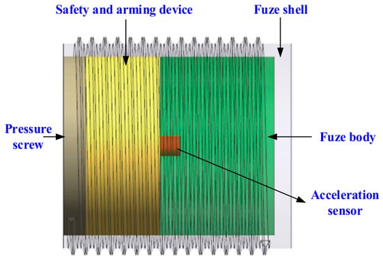
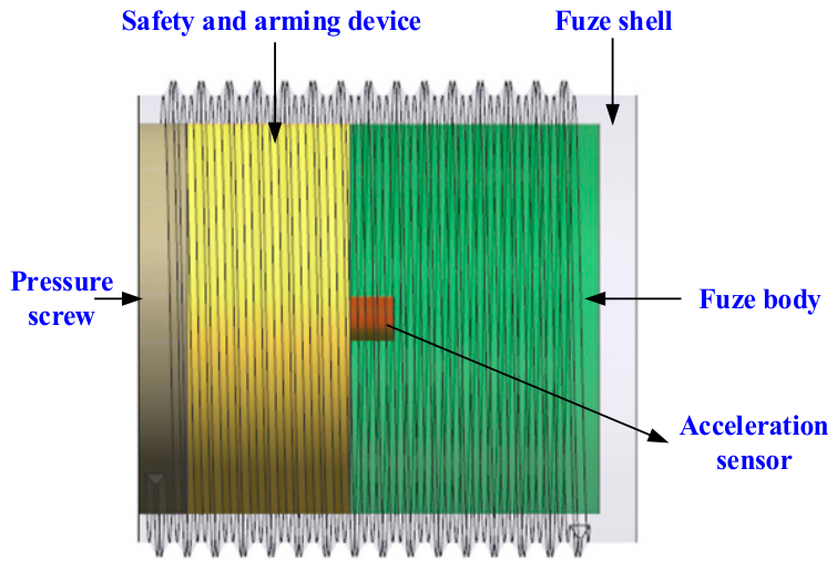
As shown in Figure 5, a typical penetration fuze structure is modeled. It can be seen that the penetration fuze is a complex system composed of the fuze shell, fuze body, pressure screw, safety and arming device, acceleration sensor, electronic module, and the buffering and sealing structure. It is extremely difficult to directly conduct dynamic modeling for such a complex structure. Therefore, an MDOF lumped parameter model will be established by analyzing the connection relationships among the various components of the fuze.

Figure 5. Penetration fuze structure.

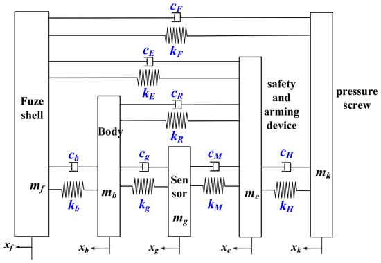
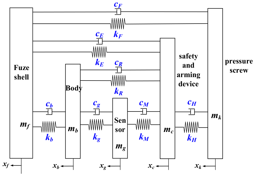
When establishing the dynamic governing equation of the fuze using the concept of lumped parameters, the fuze shell, fuze body, pressure screw, safety and arming device, acceleration sensor, and electronic module are assumed to be rigid bodies, with their mass concentrated at one point. The elastic moduli of the buffering and potting materials are far smaller than those of metallic components. They are represented as spring–damper elements in the model to transfer loads between metallic parts. Therefore, the fuze system can be simplified as an MDOF system, as shown in Figure 6.

Figure 6. MDOF model of fuze system.

The MDOF dynamic equation of the penetration fuze system can be formulated as follows:

$$\left\{\begin{array}{l}{m}_f{\ddot{x}}_f+c_b\left({\dot{x}}_f-{\dot{x}}_b\right)+k_b\left(x_f-x_b\right)+c_F\left({\dot{x}}_f-{\dot{x}}_k\right)+k_b\left(x_f-x_k\right)\\ +c_E\left({\dot{x}}_f-{\dot{x}}_c\right)+k_E\left(x_f-x_c\right)=0\\ m_b{\ddot{x}}_b-c_b\left({\dot{x}}_f-{\dot{x}}_b\right)-k_b\left(x_f-x_b\right)+c_g\left({\dot{x}}_b-{\dot{x}}_g\right)+k_g\left(x_b-x_g\right)\\ +c_R\left({\dot{x}}_b-{\dot{x}}_c\right)+k_R\left(x_b-x_c\right)=0\\ m_g{\ddot{x}}_g-c_g\left({\dot{x}}_b-{\dot{x}}_g\right)-k_g\left(x_b-x_g\right)+c_M\left({\dot{x}}_g-{\dot{x}}_c\right)+k_M\left(x_g-x_c\right)=0\\ m_c{\ddot{x}}_c-c_M\left({\dot{x}}_g-{\dot{x}}_c\right)-k_M\left(x_g-x_c\right)-c_E\left({\dot{x}}_f-{\dot{x}}_c\right)-k_E\left(x_f-x_c\right)\\ -c_R\left({\dot{x}}_b-{\dot{x}}_c\right)-k_E\left(x_b-x_c\right)+c_H\left({\dot{x}}_c-{\dot{x}}_k\right)+k_H\left(x_c-x_k\right)=0\\ m_k{\ddot{x}}_k-c_F\left({\dot{x}}_f-{\dot{x}}_k\right)-k_F\left(x_f-x_k\right)-c_H\left({\dot{x}}_c-{\dot{x}}_k\right)-k_H\left(x_c-x_k\right)=0\end{array}\right.$$

(43)

Writing the above equation in matrix form yields

$${\mathit{M}}_f{\ddot{\mathit{u}}}_f+{\mathit{C}}_f{\dot{\mathit{u}}}_f+{\mathit{K}}_f{\mathit{u}}_f={\mathit{F}}_f\left(t\right),$$

(44)

where ${\mathit{F}}_f$ represents the load excitation on the fuze system. The mass matrix ${\mathit{M}}_f$, displacement vector ${\mathit{u}}_f$, damping matrix ${\mathit{C}}_f$ and stiffness matrix ${\mathit{K}}_f$ of the fuze system are given by

$$\begin{array}{c}{\mathit{M}}_f=diag\left(m_f,m_b,m_g,m_c,m_k\right), {\mathit{u}}_f={\left(x_f,x_b,x_g,x_c,x_k\right)}^T\\ {\mathit{C}}_f=\left[\begin{array}{ccccc}{c}_b+c_F+c_E& -c_b& 0& -c_E& -c_E\\ -c_b& c_b+c_g+c_R& -c_g& -c_R& 0\\ 0& -c_g& c_g+c_M& -c_M& 0\\ -c_E& -c_R& -c_M& c_M+c_E+c_H+c_R& -c_H\\ -c_F& 0& 0& -c_H& c_F+c_H\end{array}\right],\\ {\mathit{K}}_f=\left[\begin{array}{ccccc}{k}_b+k_F+k_E& -k_b& 0& -k_E& -k_E\\ -k_b& k_b+k_g+k_R& -k_g& -k_R& 0\\ 0& -k_g& k_g+k_M& -k_M& 0\\ -k_E& -k_R& -k_M& k_M+k_E+k_H+c_R& -k_H\\ -k_F& 0& 0& -k_H& k_F+k_H\end{array}\right]\end{array}$$

(45)

where $k_F$ and $c_F$ are the equivalent stiffness and damp of the thread between the fuze shell and pressure screw, respectively. $k_E$ and $c_E$ are the equivalent stiffness and damp of the cushion collar. $k_b$ and $c_b$ are the equivalent stiffness and damp of the spacer. $k_g$ and $c_g$ are the equivalent stiffness and damp of the potting adhesive. $k_M$ and $c_M$ are the equivalent stiffness and damp between the acceleration sensor and the safety and arming device. $k_H$ and $c_H$ are the equivalent stiffness and damp between the safety and arming device and the pressure screw.

3.5. Coupled Dynamic Model of Penetrating Projectile–Fuze System

Through the above analysis, the projectile penetration resistance, the dynamic equation of coupled projectile–charge structure, and the MDOF lumped parameter model of the penetration fuze system have been established. These models lay the necessary foundation for developing a coupled dynamic model of the penetration projectile–fuze system that covers the complete chain from the projectile–target interaction to the response of the penetration fuze system. To establish the connection between the penetration fuze and the penetration projectile–charge structure, the penetration fuze system is treated as an “additional substructure”. Through coupling modeling and continuity conditions, the projectile–charge coupled structure and the penetration fuze system are integrated into a unified one. Consequently, the overall coupled dynamic model of the penetration projectile–fuze system is developed and solved globally. According to this approach, the degrees of freedom of the penetration projectile–fuze system are redefined as

$$\mathit{U}={\left(x_1,x_2,x_3\cdots x_m\right)}^T=\left(\begin{array}{l}{\mathit{u}}_b\\ {\mathit{u}}_f\end{array}\right)={\left(u_1,u_2,u_3\cdots u_N,x_f,x_b,x_g,x_c,x_k\right)}^T.$$

(46)

Then, the final form of the coupled nonlinear dynamic equation for the penetration projectile–fuze system is established as

$$\left({\mathit{M}}_t+{\mathit{M}}_r+{\mathit{M}}_f\right)\ddot{\mathit{U}}+\left({\mathit{C}}_b+{\mathit{C}}_f+{\mathit{C}}_c\right)\dot{\mathit{U}}+\left({\mathit{K}}_b+{\mathit{K}}_f+{\mathit{K}}_c\right)\mathit{U}=\mathit{F}\left(t\right),$$

(47)

where ${\mathit{C}}_c$ and ${\mathit{K}}_c$ are the coupled damp matrix and coupled stiffness matrix, respectively, which describe the connection between the projectile and fuze. $\mathit{U}$ and $\mathit{F}\left(t\right)$ represent the global displacement matrix and external load excitation of the penetration projectile–fuze system, respectively. The external load excitation can be expressed as $\mathit{F}\left(t\right)={\left(\begin{array}{cc}{\mathit{F}}_b& \mathbf{0}\end{array}\right)}^T={\left(F\left(t\right),0,0\cdots 0,0,0,0,0,0\right)}^T$. Since many symbols are used in the above Sections, please refer to Appendix A for the relevant nomenclature.

3.6. Parameter Determination of the Dynamic Model

(1)

Proportional damping coefficients of projectile–charge structure

The damping matrix of the projectile–charge coupled structure is modeled as Rayleigh proportional damping, in which the damping matrix is constructed as a linear combination of the mass and stiffness matrices.

$${\mathit{C}}_b=\alpha \left({\mathit{M}}_t+{\mathit{M}}_r\right)+\beta {\mathit{K}}_b$$

(48)

where $\alpha$ and $\beta$ are mass-proportional and stiffness-proportional damping coefficients, respectively. This approach assumes that the modal damping distribution follows the global dynamic behavior of the structure and is widely adopted in engineering practice for complex structural systems.

The coefficients $\alpha$ and $\beta$ are determined from the first two natural frequencies of the coupled structure. Let ${\omega }_1$ and ${\omega }_2$ be the first two natural circular frequencies, and ${\xi }_1$ and ${\xi }_2$ the corresponding modal damping ratios. According to the orthogonality condition of mode shapes, the following formula is obtained:

$${\xi }_i={\displaystyle \frac{\alpha }{2{\omega }_i}}+{\displaystyle \frac{\beta {\omega }_i}{2}},\left(i=1,2\right)$$

(49)

Solving the above formula yields

$$\alpha ={\displaystyle \frac{2\xi {\omega }_1{\omega }_2}{{\omega }_1+{\omega }_2}},\beta ={\displaystyle \frac{2\xi }{{\omega }_1+{\omega }_2}},\left({\xi }_1={\xi }_2=\xi \right).$$

(50)

In the present work, a modal damping ratio of 0.01 is adopted for the projectile–charge coupled structure. The natural frequencies of this structure can be estimated by the following formula:

$$f_n={\displaystyle \frac{n}{2L}}\sqrt{{\displaystyle \frac{E_{eff}^{*}{A}_{eff}^{*}}{{\rho }_{eff}{A}_{eff}}}}$$

(51)

where $n$ denotes the order of the natural frequency. $L$ is the length of the projectile.

(2)

Equivalent stiffness and damp of threaded connection

Usually, the projectile and the fuze are connected by threads. Due to the complexity of the threaded structure, equivalent stiffness and damping properties are generally approximated. Zhang et al. [29] proposed an elastic model for the threaded connection structure and provided a calculation method for the equivalent stiffness. According to their theory, the equivalent stiffness of the threaded connection structure can be expressed as

$$k_{thread}={\displaystyle \frac{\cos \left(\lambda L_{thread}\right)-1}{\sin \left(\lambda L_{thread}\right)}}{\displaystyle \frac{E_m{E}_n}{\lambda \tan {\alpha }_{thread}\left(k_n{E}_m+k_m{E}_n\right)}},$$

(52)

where $E_n$ and $E_m$ are the elasticity modulus of internal and external threads of the thread connection structure, respectively. $\lambda$ represents the axial load distribution coefficient. $L_{thread}$ and $\alpha$ are the engagement length and helix angle, respectively. $k_n$ and $k_m$ are the axial stiffness per unit length [29]. The damping of the threaded connection mainly originates from the frictional dissipation induced by micro-slip at the thread engaging surfaces. In this paper, the empirical damping ratio is adopted to characterize the damping property of the threaded interface [34], that is,

$$c_{thread}=2{\xi }_{thread}\sqrt{m_{e\mathit{q}}{k}_{thread}},$$

(53)

where ${\xi }_{thread}$ and $m_{e\mathit{q}}$ are the damping ratio and equivalent mass of the threaded connection, respectively. The damping of threaded connections is affected by multiple factors such as preload and excitation amplitude, and its parameters exhibit significant uncertainty, which cannot be accurately solved by theoretical analysis [41]. According to [42], the damping ratio of the threaded connection ranges from 0.01 to 0.03, and the value of 0.01 is adopted in the calculation.

(3)

Equivalent stiffness and damp of viscous materials

The fuze structure consists of metallic and viscous materials. Since the elastic modulus of metals is much larger than that of viscous materials, metallic components are treated as rigid bodies. The elastic restoring force (i.e., stiffness) and damping of the structure are mainly contributed by the viscous materials. The fuze shell, body, safety and arming device and pressure screw are metallic parts. The non-metallic materials are mainly PTFE and epoxy resin, which serve for buffering and potting.

In the fuze system, PTFE is adopted as the buffer material for the interfaces between the fuze shell and body, the fuze shell and safety and arming device, and the body and safety and arming device. Therefore, the corresponding equivalent stiffness and damping can be determined based on the structural and mechanical parameters of PTFE. For PTFE materials, the equivalent stiffness is

$$k_{PTFE}={\displaystyle \frac{E_{PTFE}{A}_{PTFE}}{h_{PTFE}}},$$

(54)

where $E_{PTFE}$ represents the dynamic elasticity modulus of PTFE in compression. In this study, the dynamic elastic modulus of PTFE is taken as 1.2 GPa. $A_{PTFE}$ and $h_{PTFE}$ are the effective contact area and thickness of PTFE, respectively. The damping property is characterized by the loss factor $\tan \delta$. Under the approximation that the excitation frequency is close to the natural frequency of the element, the equivalent damping ratio can be converted from the loss factor [43], i.e., ${\xi }_{PTFE}=0.5\tan \delta$.

In the fuze system, epoxy resin is used for potting. During high-speed penetration, epoxy resin is subjected to high strain rate deformation. Therefore, the ZWT nonlinear viscoelastic constitutive model [44] is adopted to describe its mechanical properties. The complete constitutive equation of the ZWT model is given by

$$\sigma \left(t\right)={\sigma }_e\left(\epsilon \left(t\right)\right)+E_1{\displaystyle {\int }_0^t\dot{\epsilon }\left(\tau \right)\exp \left(-\frac{t-\tau }{{\theta }_1}\right)d\tau }+E_2{\displaystyle {\int }_0^t\dot{\epsilon }\left(\tau \right)\exp \left(-\frac{t-\tau }{{\theta }_2}\right)d\tau },$$

(55)

where $\sigma \left(t\right)$ is the nonlinear elastic equilibrium response and $\epsilon \left(t\right)$ is strain. $E_1$ and ${\theta }_1$ denote the elastic constant and relaxation time of the low-frequency Maxwell element, respectively. $E_2$ and ${\theta }_2$ denote the elastic constant and relaxation time of the low-frequency Maxwell element, respectively. The value of these parameters is given in [44]. The high-frequency Maxwell element undergoes significant relaxation under impact loading, so its integral term can degenerate into a pure damping term, i.e., $E_1{\displaystyle {\int }_0^t\dot{\epsilon }\left(\tau \right)\exp \left(-\frac{t-\tau }{{\theta }_1}\right)d\tau }\approx {\eta }_2\dot{\epsilon }\left(t\right)=E_2{\theta }_2$. Under small deformations, the nonlinear elastic response can be linearized as ${\sigma }_e\left(\epsilon \right)=E_0\epsilon$. $E_0$ denotes the initial elastic modulus. Therefore, the linearized form of the ZWT constitutive model under high strain rate conditions is given by

$$\sigma \left(t\right)=\left(E_0+E_1\right)\epsilon \left(t\right)+{\eta }_2\dot{\epsilon }\left(t\right)=E_{\infty }\epsilon \left(t\right)+E_2{\theta }_2\dot{\epsilon }\left(t\right),$$

(56)

where $E_{\infty }$ represents the steady-state elastic modulus. ${\eta }_2=E_2{\theta }_2$ is the dynamic viscosity. Assuming that the thickness of epoxy resin is $h$ and its deformation under impact loading is $x$, then $\sigma \left(t\right)=E_{\infty }{\displaystyle \frac{x}{h}}+E_2{\theta }_2{\displaystyle \frac{\dot{x}}{h}}$. Hence, the restoring force of the epoxy resin due to compression is

$$F=\sigma \left(t\right)A_e={\displaystyle \frac{E_{\infty }{A}_e}{h}}x+{\displaystyle \frac{E_2{\theta }_2}{h}}\dot{x}.$$

(57)

Therefore, the stiffness and damp of epoxy resin can be obtained as follows:

$$k_{Epoxy}={\displaystyle \frac{E_{\infty }{A}_e}{h}};c_{Epoxy}={\displaystyle \frac{A_e{E}_2{\theta }_2}{h}}$$

(58)

3.7. Solution for Coupled Dynamic Model of Penetrating Projectile–Fuze System

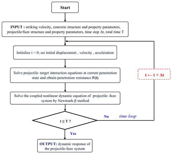
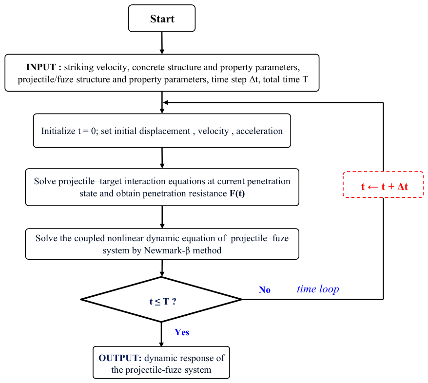
Equation (47) is a second-order differential equation which cannot be solved analytically and thus requires numerical solution. For the dynamic equation in the above form, the Newmark-β time integration method with $\gamma =0.5$ and $\beta =0.25$ is adopted. This parameter choice guarantees zero numerical dissipation in the integration process. In addition, a fixed time step of 10⁻⁷ s is used throughout the simulation. The computational flowchart is given in Figure 7.

Figure 7. Solution flowchart for coupled projectile–fuze dynamic model.

4. Results and Discussion

In this section, the dynamic responses of a projectile–fuze system penetrating a finite-thickness concrete target will be investigated. The parameters of the penetration warhead and fuze are given in Table 1 and Table 2, respectively. It should be noted that the shear modulus and Young’s modulus of the charge in Table 1 satisfy the relation $E=2G\left(1+\mu \right)$, where $G$ and $E$ are the shear modulus and Young’s modulus, respectively, and $\mu$ denotes Poisson’s ratio. In addition, the thread specification of the projectile–fuze threaded connection is M100 × 3, and the thread engagement length is 86 mm. The thread specification of the pressure screw is M85 × 2, and the engagement length is 25 mm. The parameters of buffering and potting structures are given in Table 3 and Table 4.

Table 1. Parameters of penetration warhead.

Projectile		Charge
Parameter	Value	Parameter	Value
Diameter (mm)	360	Diameter (mm)	320
Length (mm)	2100	Length (mm)	1650
Ogive nose radius (mm)	3060	Density (kg/m3)	1700
Ogive nose length (mm)	574	Shear modulus (GPa)	5
Density (kg/m3)	7800	Poisson’s ratio	0.32
Young’s modulus (GPa)	210	Young’s modulus (GPa)	13.2
Poisson’s ratio	0.284

Table 2. Parameters of fuze.

Parameter	Value (kg)	Parameter	Value (kg)
Mass of fuze shell	1.38	Mass of safety and arming device	0.32
Mass of body	0.5	Mass of acceleration sensor	0.05
Mass of pressure screw	0.16

Table 3. Parameters of buffering structures.

Parameter	Value	Parameter	Value
Height of spacer	2 mm	Height of cushion collar	44 mm
Diameter of spacer	78 mm	Inner/outer diameter of cushion collar	78 mm/82 mm

Table 4. Parameters of potting structures.

Parameter	Value	Parameter	Value
Height of potting adhesive	33 mm	Diameter of potting adhesive	62 mm

4.1. Model Validation

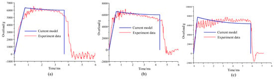
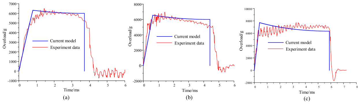
To validate the projectile–target interaction model presented in Section 3.2, the overload calculated by the model is compared with the experimental data from Forrestal et al. [45], who measured the overload of ogive-nose projectiles normally penetrating thick concrete targets. For comparison, the projectile parameters corresponding to the experiments are adopted, with projectile striking velocity of 200 m/, 250 m/s and 379 m/s. The compressive strength of concrete is 23 MPa and the CRH (caliber radius head) of the projectile is 3.0. The ogive-nose projectile parameters are given in Table 5. The comparison results are presented in Figure 8 and Table 6. As shown in Figure 8 and Table 6, it can be observed that the overload of the projectile calculated by the current model is in agreement with the experiments conducted by Forrestal et al. [45].

Table 5. Ogive-nose projectile parameters [45].

No.	Projectile Mass (kg)	Striking Velocity (m/s)	Projectile Diameter (mm)	Target Length (m)	R (MPa)
1	13.037	200	76.2	1.83	161
2	13.085	250	76.2	1.22	158
3	13.119	379	76.2	1.83	171

Figure 8. Comparison of projectile overload between experiments [45] and calculation. (a) Projectile striking velocity 200 m/s, CHR = 3.0. (b) Projectile striking velocity 250 m/s, CHR = 3.0. (c) Projectile striking velocity 379 m/s, CHR = 3.0.

Table 6. Quantitative comparison of projectile overload between experiments [45] and calculation.

No.	Overload Peak (g)			Penetration Time (ms)
	Experiment	Theory	Error (%)	Experiment	Theory	Error (%)
1	6525.70	6320.09	3.15	4.08	3.76	7.84
2	7135.51	6586.45	7.69	4.74	4.42	6.75
3	7918.22	7739.49	2.26	6.09	5.88	3.45

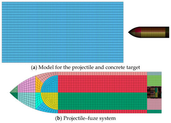
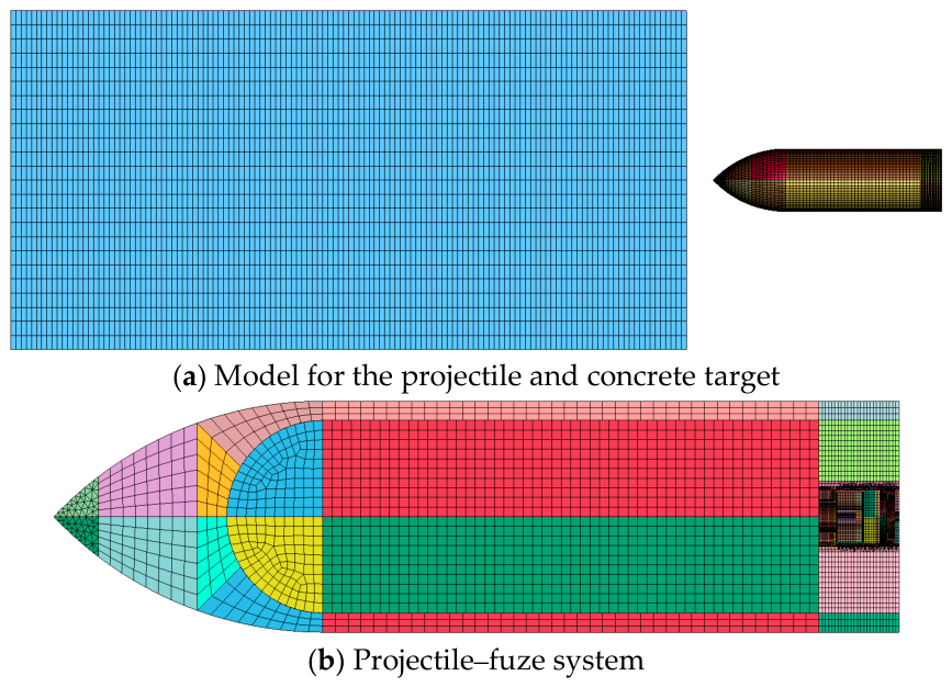
Furthermore, to verify the coupling dynamics model of the penetration projectile–fuze system presented in Section 3.5, the overload response of the fuze evaluated by the presented model will be compared with that obtained by LS-DYNA software. For comparison, it is assumed that a projectile normally strikes a concrete target with 9 m at a high velocity of 810 m/s. Figure 9 shows the FE numerical simulation model of the projectile–fuze system.

Figure 9. FE numerical simulation model of projectile–fuze system.

The projectile is made of high-strength alloy steel and follows the Johnson–Cook constitutive model, which is defined by the keyword “*MAT_JOHNSON_COOK”. The specific parameters are shown in Table 7.

Table 7. Projectile parameters based on JC constitutive model (cm-g-μs-K).

Elasticity Modulus	Density	Poisson’s Ratio	Quasi-Static Yield Strength	Strain Hardening Coefficient	Strain Hardening Exponent	Strain Rate Sensitivity Coefficient	Thermal Softening Exponent
2.11	7.85	0.28	0.01327	0.512	0.232	0.0034	1.27

The charge is described by the isotropic elastoplastic constitutive model with the keyword “*MAT_ISOTROPIC_ELASTIC_PLASTIC”. The corresponding parameter settings are shown in Table 8.

Table 8. Parameter setting of charge (cm-g-μs-K).

Shear Modulus	Density	Yield Stress	Plastic Tangent Hardening Modulus	Bulk Modulus
0.1	1.73	0.0005	0.0067	0.02

The material of the fuze shell and pressure screw is TC4. The fuze body and safety and arming device are made of aluminum alloy. The bilinear kinematic elastoplastic constitutive model is adopted, which is defined by the keyword “*MAT_PLASTIC_KINEMATIC” in the software. The parameter settings of fuze shell, fuze body, safety and arming device are given in Table 9 and Table 10.

Table 9. Parameters of TC4—(cm-g-μs).

Elasticity Modulus	Density	Poisson’s Ratio	Static Initial Yield Stress	Hardening Parameter
1.1	4.4	0.31	0.011	1

Table 10. Parameters of aluminum alloy (cm-g-μs).

Elasticity Modulus	Density	Poisson’s Ratio	Static Initial Yield Stress	Hardening Parameter
0.7	2.7	0.33	0.007	1

The HJC constitutive model is used for the concrete target, which is defined by the keyword “*MAT_JOHNSON_HOLMQUIST_COOK” in the software. The parameter setting is given in Table 11.

Table 11. Parameter setting of concrete target (cm-g-μs-K).

Density	Shear Modulus	Normalized Cohesive Strength	Normalized Pressure Hardening Coefficient	Strain Rate Coefficient	Pressure Hardening Exponent	Quasi-Static Uniaxial Compressive Strength
2.5	0.167	0.69	1.5	0.007	0.61	0.0004
Maximum Tensile Hydrostatic Pressure	Reference Strain Rate	Minimum Plastic Strain for Damage Accumulation	Normalized Maximum Strength	Crushing Pressure	Crushing Volumetric Strain	Locking Pressure
0.00004	0.000006	0.01	7	0.00016	0.001	0.008
Locking Volumetric Strain	Damage Constant D1	Damage Constant D2	Pressure Constant K1	Pressure Constant K2	Pressure Constant K3	Failure Erosion Strain
0.1	0.04	1	0.85	−1.71	2.08	0.15

A tied contact is established between the projectile and charge. The threaded connections adopt the automatic surface-to-surface contact defined by the keyword “*CONTACT_AUTOMATIC_SURFACE_TO_SURFACE”. The relevant setting is given in Table 12.

Table 12. Model contact interface and friction parameter.

Contact Pair	LS-DYNA Keyword	Contact Type	Friction Setting
Projectile–charge	CONTACT_TIED	Tied contact	–
Threaded connection	CONTACT_AUTOMATIC_SURFACE_TO_SURFACE	Automatic surface-to-surface contact	0.15

The boundary condition adopted in the simulation is illustrated in Table 13.

Table 13. Boundary condition.

Model Component	Constraint Type	Constraint Description
Concrete target	Full fixed constraint	Fixed constraints are applied to the target plate to restrict all translational and rotational degrees of freedom.
Projectile–fuze system	Free boundary	No displacement constraints

Moreover, the local mesh refinement is performed in the penetration area and threaded connection regions. The model is meshed by a zonal discretization strategy. After fine meshing processing, the total number of elements of the numerical model reaches 676,575. The results are given in Figure 10 and Table 14.

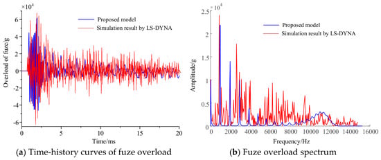
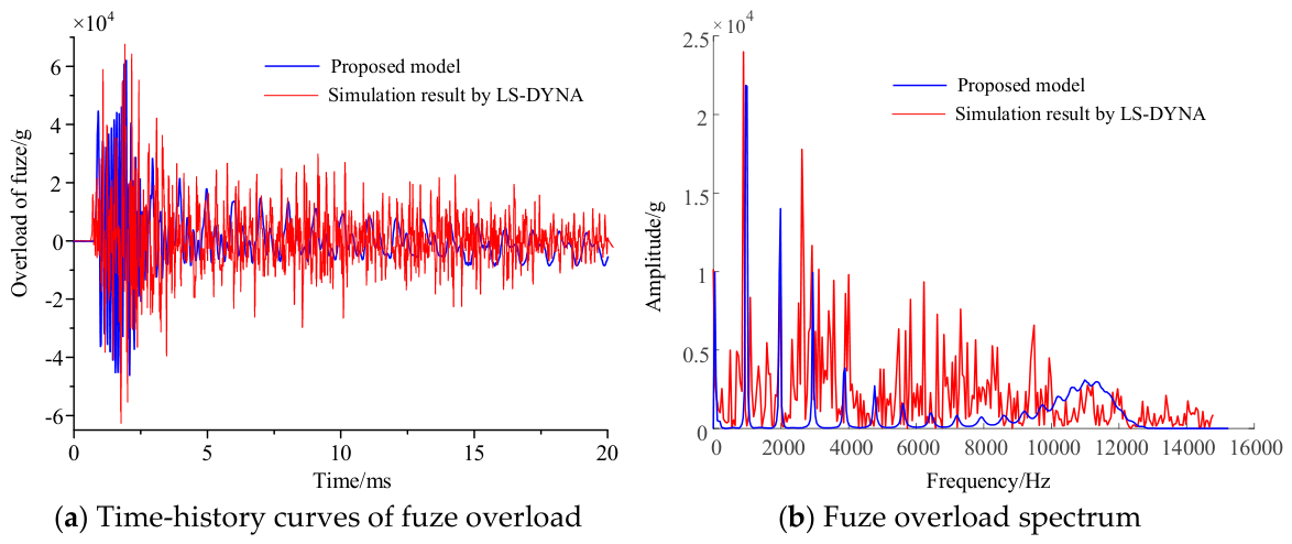
Figure 10. Comparison of overload response of fuze between LS-DYNA simulation and dynamic model calculation.

Table 14. Peak value comparison between LS-DYNA simulation and model calculations.

Parameter	LS-DYNA Simulation	Dynamic Model Calculation	Error (%)
Positive peak (g)	67,910	63,068	7.13
Negative peak (g)	62,153	46,375	25.38

Figure 10 shows the comparison of time-history curves of fuze overload, while Table 14 lists the quantitative comparison of overload peaks. As shown in Figure 10a, it is noticed that the overall trend of overload from the dynamic model is consistent with LS-DYNA simulation. The relative error of the positive overload peak is only 7.13%, and the relative error of the negative peak reaches 25.38%. As shown in Figure 10b, the main peak positions of the fuze overload spectrum obtained from the theoretical model generally coincide with the LS-DYNA simulation results. These frequency values correspond exactly to the first three natural frequencies of the system, namely 936.37 Hz, 1872.74 Hz and 2809.11 Hz. This indicates that the proposed theoretical model can effectively characterize the low-order inherent vibration characteristics of the projectile–fuze system. Nevertheless, the LS-DYNA simulation signal contains abundant high-frequency components, which cannot be reproduced by the theoretical model. Generally speaking, the theoretical model can capture the primary inherent vibration characteristics of the fuze system, although discrepancies still exist in the amplitude at high frequencies. In fact, the theoretical model cannot be as detailed as the simulation model. The simulation model can achieve refined grid division during the calculation and can also simulate the collision of threaded connections as well as the propagation and reflection of stress waves in different structures and interfaces. Therefore, there are deviations between the results of the theoretical model and the simulation.

4.2. Motion Characteristics of Projectile

In this section, the motion characteristics of the projectile will be studied based on the interaction model of the projectile–target presented in Section 3.2.

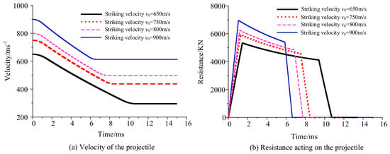
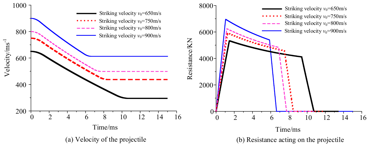
Figure 11 describes the influence of striking velocity on the penetration velocity and resistance of the projectile, and Table 15 presents the quantitative comparison of key indicators under different striking velocities. The thickness of the concrete target is 6 m and the target’s compressive strength is 40 Mpa. As shown in Figure 11 and Table 15, it can be clearly observed that the motion state is highly affected by the striking velocity of the projectile. As the striking velocity of the projectile increases, the residual velocity increases, while the penetration time decreases. The resistance peak of the projectile increases significantly with the increase in striking velocity. Meanwhile, the duration of each penetration stage tends to decrease, and the durations of the cratering stage, tunneling stage and shear plugging stage all reduce as the striking velocity increases. In addition, although the increase in striking velocity raises the penetration resistance, the velocity loss of the projectile decreases instead. The reason is that the higher the impact velocity, the greater the interaction between the projectile and target, and the penetration resistance increases accordingly. However, the duration of projectile–target interaction significantly shortens, and the total energy dissipated by the target decreases, thus resulting in less projectile velocity loss.

Figure 11. The effect of striking velocity on the penetration velocity and resistance of the projectile.

Table 15. Quantitative comparison of the effects of striking velocity.

Striking Velocity (m/s)	Residual Velocity (m/s)	Resistance Peak (KN)	Duration of Cratering Stage (ms)	Duration of Tunneling Stage (ms)	Duration of Shear Plugging Stage (ms)
650	295	5324	1.45	7.65	1.38
750	437	5908	1.29	6.23	0.99
800	498	6257	1.20	5.71	0.86
900	612	6972	1.04	4.88	0.73

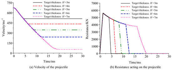
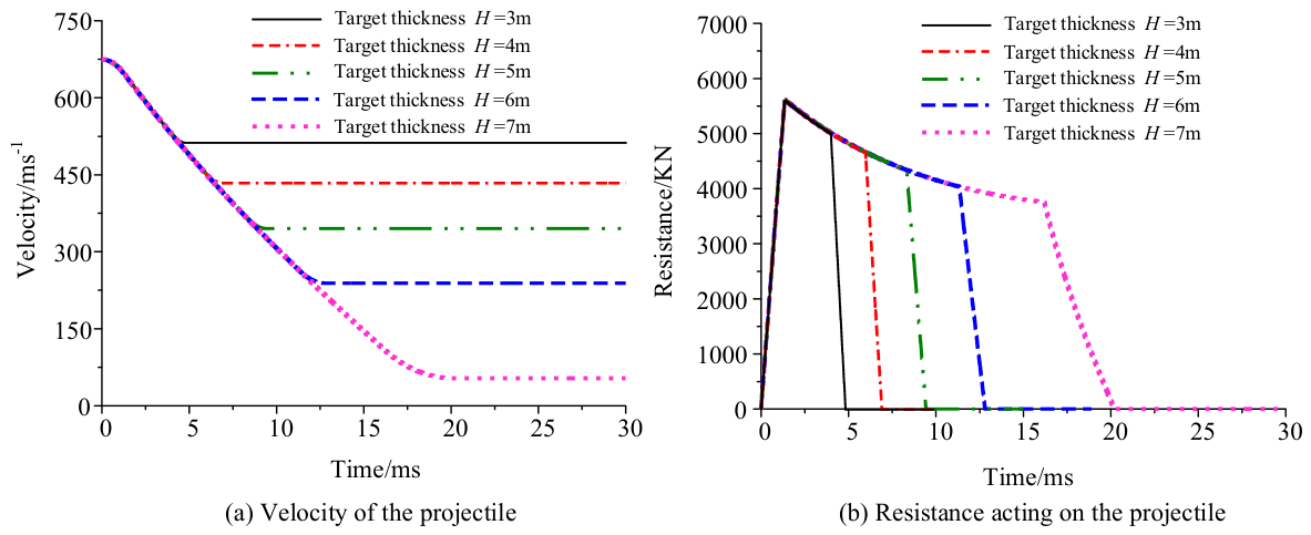
Figure 12 and Table 16 illustrate the effect of concrete target thickness on the penetration velocity and penetration resistance of the projectile. The concrete’s strength is C40, the impact velocity is 810 m/s, and the target thicknesses are 3, 4, 5, 6, and 7 m. The results show that the target thickness has almost no effect on the penetration resistance peak and the duration of the cratering stage. However, as target thickness increases, the durations of the tunneling stage and shear plugging stage extend markedly. Meanwhile, the residual velocity of the projectile decreases significantly as the target thickness increases. In fact, the increase in target thickness merely lengthens the loaded distance of the projectile within the penetration region. The instantaneous penetration resistance peak remains unchanged, while the prolonged interaction consumes more kinetic energy of the projectile and ultimately reduces the residual velocity.

Figure 12. The effect of target thickness on the penetration velocity and resistance of the projectile.

Table 16. Quantitative comparison of the effects of target thickness.

Target Thickness (m)	Residual Velocity (m/s)	Resistance Peak (KN)	Duration of Cratering Stage (ms)	Duration of Tunneling Stage (ms)	Duration of Shear Plugging Stage (ms)
3	537	5624	1.27	2.80	0.75
4	458	5624	1.27	4.79	0.91
5	370	5624	1.27	7.11	1.06
6	263	5624	1.27	10.11	1.46
7	78	5624	1.27	14.95	3.98

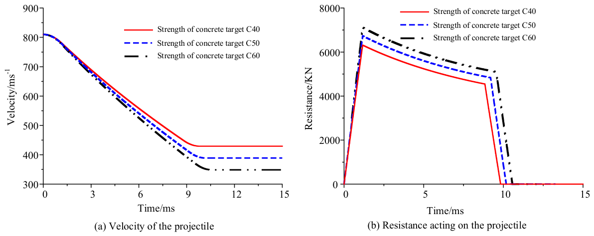
Figure 13 and Table 17 show the dependence of the penetration velocity and resistance of the projectile on the compressive strength of the concrete target. The striking velocity of the projectile is 810 m/s, the target thickness is 6 m, and the target strength levels are C40, C50, and C60. It can be seen that as the strength of the concrete target increases, the penetration resistance peak increases, and the duration of the cratering stage remains basically constant. The duration of the tunneling stage increases slightly, while the variation in the shear plugging stage duration is negligible. The residual velocity of the projectile decreases significantly. This is because higher-strength concrete has stronger anti-penetration capacity, which increases the resistance of projectile–target interaction. Under the same impact conditions, the target dissipates more kinetic energy of the projectile, leading to a reduction in the projectile residual velocity.

Figure 13. Penetration velocity and axial resistance of projectile under different target strength.

Table 17. Quantitative comparison of the effects of concrete strength.

Target Strength (MPa)	Residual Velocity (m/s)	Resistance Peak (KN)	Duration of Cratering Stage (ms)	Duration of Tunneling Stage (ms)	Duration of Shear plugging Stage (ms)
40	429	6306	1.17	7.67	1.02
50	389	6717	1.17	8.05	0.96
60	348	7105	1.17	8.37	1.02

During high-velocity penetration, the friction between the projectile and concrete target is governed by coupled effects of aggregate properties, impact pressure, and material fragmentation. It cannot be easily measured in tests and no universally accepted value is available. Therefore, the friction coefficient is only adopted as a variable input parameter for analysis.

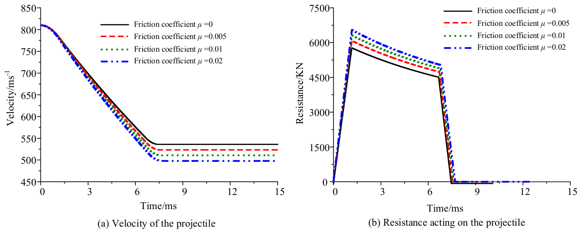
Figure 14 and Table 18 present the influence of the friction coefficient on the penetration velocity and axial resistance of the projectile. The striking velocity of the projectile is 810 m/s, the concrete thickness is 5 m, and the target strength is C40. It can be observed that the variation in the friction coefficient barely affects the duration of the cratering stage. As the friction coefficient increases, the penetration resistance peak increases, the durations of the tunneling stage and shear plugging stage increase slightly, and the residual velocity of the projectile decreases accordingly. This is because friction of the projectile brings additional axial resistance. A larger friction coefficient contributes higher frictional resistance and more kinetic energy dissipation; thus, the residual velocity of the projectile reduces.

Figure 14. Penetration velocity and axial resistance of projectile considering influence of friction.

Table 18. Quantitative comparison of effects of friction coefficient.

Friction Coefficient	Residual Velocity (m/s)	Resistance Peak (KN)	Duration of Cratering Stage (ms)	Duration of Tunneling Stage (ms)	Duration of Shear plugging Stage (ms)
0	536	5831	1.16	5.52	0.78
0.005	523	6063	1.16	5.56	0.81
0.01	511	6311	1.16	5.59	0.88
0.02	498	6566	1.16	5.65	0.91

4.3. Dynamic Characteristics of Projectile–Fuze System

In this section, the overload characteristics of the fuze under different influencing factors will be further discussed based on the coupled dynamic model of the penetrating projectile–fuze system presented in Section 3.

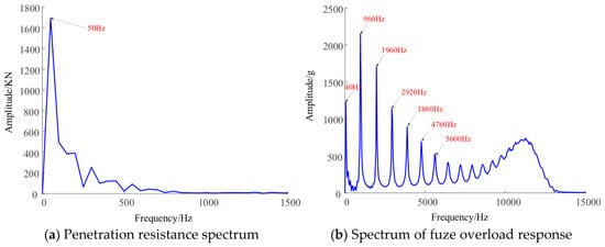
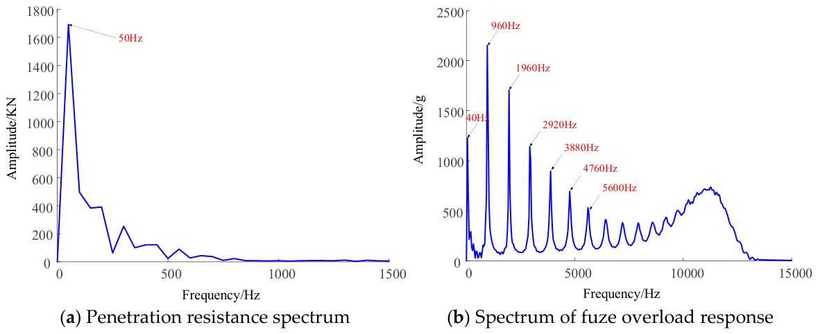
To reveal the dynamic features of the projectile–fuze system under penetration, spectral analysis is carried out for penetration resistance and fuze overload. Figure 13 shows the spectra of penetration resistance and fuze overload when the projectile impacts a 6 m thick concrete target at 850 m/s. In Figure 15a, the energy concentrates within the low-frequency band, with the main peak at 50 Hz. The amplitude drops quickly as frequency rises, showing that penetration resistance is dominated by low-frequency components. In Figure 15b, the fuze overload spectrum displays a set of separate peaks at 40 Hz, 960 Hz, 1960 Hz, 2920 Hz, 3880 Hz and other positions. The peaks at 960 Hz, 1960 Hz and 2920 Hz match the first three natural frequencies of the projectile–fuze system (936.37 Hz, 1872.74 Hz, 2809.11 Hz) reasonably well. This observation indicates that although the penetration resistance is dominated by low-frequency components, the propagation of stress waves in the projectile–fuze structure excites multiple modes of the system, which accounts for the high-frequency oscillations in the fuze overload. The low-frequency component originates from the penetration resistance, while the high-frequency oscillations are governed by the inherent vibration modes of the projectile–fuze structure.

Figure 15. Frequency component of projectile–fuze system.

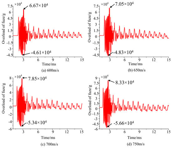
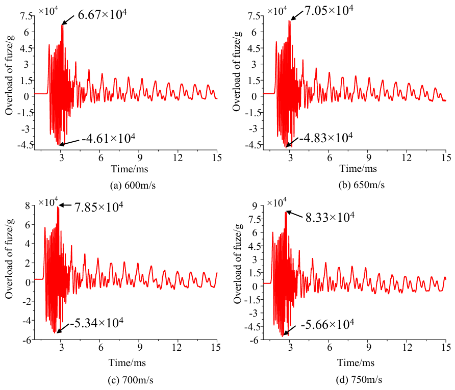
Figure 16 presents the fuze overload response at the acceleration sensor position considering the influence of projectile striking velocity. The thickness of the concrete target and its compressive strength are 6 m and 40 MPa, respectively. It can be seen that the fuze overload rapidly rises to the peak and is accompanied by violent high-frequency oscillation at the initial penetration stage. As the striking velocity increases, the overload of the fuze generally shows an increasing trend, particularly during the cratering stage and the early tunneling stage, where the peak value of overload rises significantly. Beyond the early tunneling stage, the influence of striking velocity gradually weakens, and the overload exhibits periodic oscillation induced by structural vibration. It can be seen from Figure 11 that as the striking velocity increases, the instantaneous penetration resistance rises, while the duration of projectile–target interaction is shortened, which reduces the duration of projectile–target resistance excitation. The amplitude of penetration resistance and the duration of projectile–target excitation jointly determine the time-history characteristics of fuze overload under different striking velocities.

Figure 16. Overload of fuze vs. striking velocity.

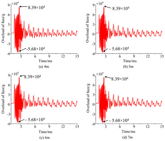
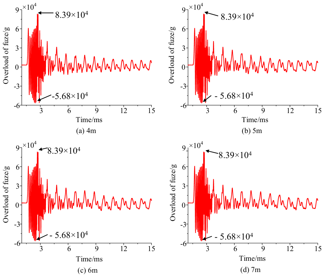
Figure 17 shows the effect of the thickness of the concrete target on the overload response of the fuze. It is noticed that the thickness of the concrete target has almost no influence on the overload response of the fuze. Notably, during the cratering stage and the early tunneling stage, target thickness hardly affects the overload response of the fuze sensor, with only a slight influence appearing after the early tunneling stage. In fact, as can be seen in Figure 10, variations in the thickness of the concrete target have little impact on the peak value of penetration resistance, but mainly affect the projectile–target interaction time. Consequently, the overload response of the fuze exhibits the behavior described above.

Figure 17. Overload of fuze vs. target thickness.

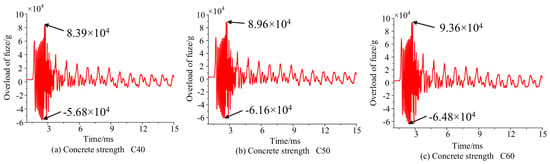
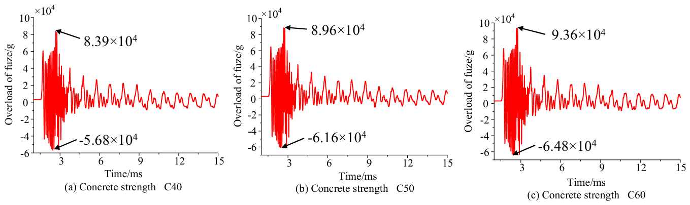
Figure 18 presents the overload responses of the fuze acceleration sensor under different concrete strengths. In the calculation, concrete targets with C40, C50, and C60 are selected. The projectile penetrates a 6 m thick concrete target at a striking velocity of 810 m/s. It can be seen that both the positive and negative peak values of fuze overload increase as the concrete strength increases. As shown in Figure 13, the higher the concrete strength, the stronger the impact load generated during the penetration process, and the overload peak of the fuze will also increase accordingly.

Figure 18. Overload of fuze vs. concrete target strength.

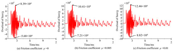
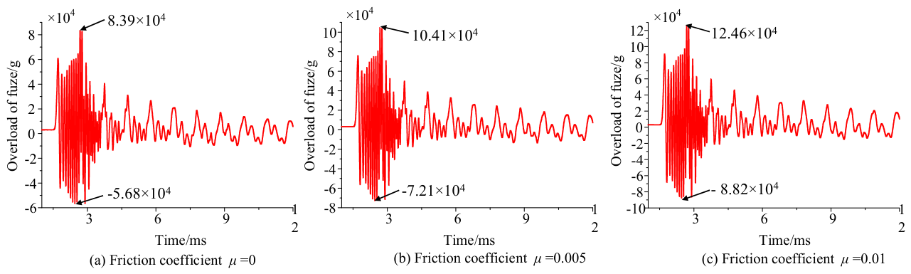
Figure 19 illustrates the overload response of the fuze acceleration sensor considering the effect of friction between the projectile and the concrete target. It is observed that the friction between the projectile and the concrete target has a significant influence on the overload peak. As the friction coefficient increases, the overload peak value of the fuze increases markedly. In fact, at the initial stage of penetration, the contact area between the projectile nose and the concrete target gradually increases, and the friction force rises accordingly, which further increases the overload peak of the fuze.

Figure 19. Overload of fuze vs. friction.

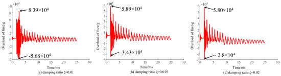
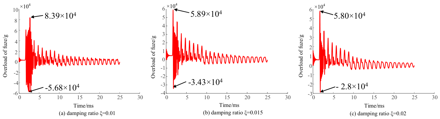
Figure 20 presents the fuze overload responses under different damping ratios. It can be observed that the damping ratio has a remarkable influence on both the overload peak and oscillation characteristics of fuze overload. As the damping ratio increases, the peak of the fuze overload response decreases, and the oscillation of the overload response curve is weakened. Damping dissipates the structural vibration energy. Larger damping can suppress the shock-induced structural vibration more rapidly and reduce the amplitude of overload oscillation.

Figure 20. Overload of fuze vs. damping ratio of projectile–charge coupled structure.

It is noted that positive/negative overload peaks and frequencies are used to characterize the penetration overload response in the above analysis, and the overload peak serves as a critical index for the high-overload-resistant design of fuze structures. Pulse duration carries important engineering value for the detonation control of penetration fuzes. Nevertheless, reliable extraction of this parameter is restricted by the inherent features of overload signals. Figure 16, Figure 17, Figure 18, Figure 19 and Figure 20 show dense high-frequency oscillations within the overload waveforms. Similar waveforms under different working conditions prevent stable identification of the start and end boundaries of overload oscillation, which impedes the analysis of how parameters affect duration. Hence, duration is not adopted as a core characteristic in this analysis.

Moreover, RMS acceleration is a key time-domain parameter commonly employed in steady-state random vibration to quantify long-term vibration energy. This work investigates short-duration transient penetration shock superimposed with high-frequency oscillations. Since fuze structural failure is governed by instantaneous overload peak, RMS acceleration cannot directly capture the peak effect of shock pulses and is rarely adopted as a core characteristic parameter in high-overload research of penetration fuzes.

5. Conclusions

To overcome the limitations in current theoretical studies and provide a reliable theoretical reference model, a comprehensive nonlinear dynamic model for projectile–fuze systems penetrating finite-thickness concrete targets has been established by considering the projectile–target interaction, projectile–charge coupling effect, fuze system and projectile–fuze coupling. On this basis, the influences of different factors on the dynamic characteristics of the penetration projectile–fuze system are further analyzed. From the above discussion and analysis, the following conclusions can be draw:

(1)

Penetration velocity and resistance are highly dependent on the striking velocity, target strength and friction. As these factors increases, the penetration resistance increases. When the striking velocity increases, the duration of the projectile–target interaction decreases, while the effect of friction shows the opposite trend.

(2)

During the penetration process, overload of the fuze exhibits severe oscillations, which are mainly concentrated in the cratering stage and the early tunneling stage. In this period, the striking velocity, target strength, friction and damping ratio have a significant impact on the overload response.

(3)

The thickness of the target primarily affects the penetration velocity and the duration of projectile–target interaction, but has almost no influence on penetration resistance. The variation in the thickness of the target has little effect on the overload response of the fuze, except that it alters the projectile–target interaction time, causing a slight change in the overload response of the fuze during the later stage of the interaction.

Admittedly, the modeling method proposed in this paper has certain limitations. On one hand, mass loss, material nonlinearity and interfacial contact nonlinearity are not included in the model. Future work will relax these assumptions to further improve the modeling framework. On the other hand, only normal penetration conditions are considered, while oblique penetration dominates most practical engineering scenarios. Under oblique impact, the projectile is subjected to additional moments and undergoes attitude deflection. Further extension of the modeling scope will be carried out to broaden the applicable range of the model. In addition, reinforced concrete targets exert a significant influence on the dynamic characteristics of the projectile–fuze system. The established model is developed for plain concrete, with reinforcement not taken into account. Hence, the effect of reinforcement should be incorporated so that the model can better reflect practical conditions.

References

- Zhang, S.; Wu, H.J.; Zhang, X.X.; Liu, J.; Huang, F. High-velocity penetration of concrete targets with three types of projectiles: Experiments and analysis. Lat. Am. J. Solids Struct. 2017, 14, 1614–1628. [Google Scholar] [CrossRef] [Scilit]
- Liu, W.; Li, R.; Niu, L.; Shi, K.L. Research status and prospect of initiation control technology for hard target penetration. Acta Armamentarii 2023, 44, 1602–1609. [Google Scholar]
- Ali, I.; Long, X. Penetration resistance of reinforced concrete slab subjected to rigid projectile impact based on finite element and analytical models. Constr. Build. Mater. 2025, 473, 140828. [Google Scholar] [CrossRef] [Scilit]
- Bishop, R.F.; Hill, R.; Mott, N.F. The theory of indentation and hardness tests. Proc. Phys. Soc. 2002, 57, 147–159. [Google Scholar]
- Hopkins, H.G. Dynamic expansion of spherical cavities in metals. In Progress in Solid Mechanics; Sneddon, I.N., Hill, R., Eds.; North-Holland: Amsterdam, The Netherlands, 1960; Volume 1, pp. 83–164. [Google Scholar]
- Forrestal, M.J.; Tzou, D.Y. A spherical cavity-expansion penetration model for concrete targets. Int. J. Solids Struct. 1997, 34, 4127–4146. [Google Scholar] [CrossRef] [Scilit]
- He, T.; Wen, H.M.; Guo, X.J. A spherical cavity expansion model for penetration of ogival-nosed projectiles into concrete targets with shear-dilatancy. Acta Mech. Sin. 2011, 27, 1001–1012. [Google Scholar] [CrossRef] [Scilit]
- Wu, H.; Fang, Q.; Zhang, Y.-D.; Gong, Z.-M. Semi-theoretical analyses of the concrete plate perforated by a rigid projectile. Acta Mech. Sin. 2012, 28, 1630–1643. [Google Scholar] [CrossRef] [Scilit]
- Sobeski, R.; Urgessa, G. Review of Quasi-Analytical and Cavity Expansion Methods for Projectile Penetration of Concrete Targets. Int. J. Prot. Struct. 2015, 6, 43–64. [Google Scholar] [CrossRef] [Scilit]
- Yankelevsky, D.Z. Resistance of a concrete target to penetration of a rigid projectile–revisited. Int. J. Impact Eng. 2017, 106, 30–43. [Google Scholar] [CrossRef] [Scilit]
- Gao, S.Q.; Liu, H.P.; Lei, J. A fuzzy model of the penetration resistance of concrete targets. Int. J. Impact Eng. 2009, 36, 644–649. [Google Scholar] [CrossRef] [Scilit]
- Warren, T.L.; Forquin, P. Penetration of common ordinary strength water saturated concrete targets by rigid ogive-nosed steel projectiles. Int. J. Impact Eng. 2016, 90, 37–45. [Google Scholar] [CrossRef] [Scilit]
- Zhang, Y.; Chen, W.; Cheng, S.; Zou, H.; Guo, Z. Penetration of rigid projectiles into concrete based on improved cavity expansion model. Struct. Concr. 2017, 18, 974–985. [Google Scholar] [CrossRef] [Scilit]
- Chen, X.; Chen, L.; Thai, H.T. An improved fractal comminution approach on the scaling effect of rigid projectile penetration into semi-infinite concrete targets. Int. J. Impact Eng. 2026, 208, 105513. [Google Scholar] [CrossRef] [Scilit]
- Rosenberg, Z.; Kositski, R. Modeling the penetration and perforation of concrete targets by rigid projectiles. Int. J. Prot. Struct. 2016, 7, 157–178. [Google Scholar] [CrossRef] [Scilit]
- Chen, X.W.; Fan, S.C.; Li, Q.M. Oblique and normal perforation of concrete targets by a rigid projectile. Int. J. Impact Eng. 2004, 30, 617–637. [Google Scholar] [CrossRef] [Scilit]
- Chen, X.W.; Li, X.L.; Huang, F.L.; Wu, H.; Chen, Y. Normal Perforation of reinforced concrete target by rigid projectile. Int. J. Impact Eng. 2008, 35, 1119–1129. [Google Scholar] [CrossRef] [Scilit]
- Duan, Z.-P.; Li, S.-R.; Ma, Z.-F.; Ou, Z.-C.; Huang, F.-L. Attitude deflection of oblique perforation of concrete targets by a rigid projectile. Def. Technol. 2020, 16, 596–608. [Google Scholar] [CrossRef] [Scilit]
- Li, P.; Zhang, X.; Wang, S.J. Trajectory characteristics of oblique penetration of projectile into concrete targets considering cratering effect. Int. J. Impact Eng. 2024, 185, 104864. [Google Scholar] [CrossRef] [Scilit]
- Booker, P.M.; Cargile, J.D.; Kistler, B.L.; La Saponara, V. Investigation on the response of segmented concrete targets to projectile impacts. Int. J. Impact Eng. 2009, 36, 926–939. [Google Scholar] [CrossRef] [Scilit]
- Zhang, D.M.; Gao, S.Q.; Niu, S.H.; Liu, H.P. Study on collision of threaded connection during impact. Int. J. Impact Eng. 2017, 106, 133–145. [Google Scholar] [CrossRef] [Scilit]
- Liu, P.; Li, J.; Li, C.; Li, H.; Zhang, J.; Zhang, H. Analysis of the influence of different initial velocities on dynamic performance of muti-layer hard target penetration process. Front. Phys. 2023, 11, 1241762. [Google Scholar] [CrossRef] [Scilit]
- Chen, B.Y.; Ma, X.; Yu, D.; Chen, C.; Dai, K.R. Dynamic modeling and simulation of projectile fuze multibody system based on Hunt-Crossley contact model. J. Nanjing Univ. Sci. Technol. 2025, 49, 412–423. [Google Scholar]
- Zhang, A.; Liu, P.; Zhang, H. Analysis and experiment of stress concentration in penetration fuze buffer materials under stress wave incursion. Front. Phys. 2024, 12, 1401538. [Google Scholar] [CrossRef] [Scilit]
- Zhang, H.; Niu, S. Analysis the influence of projectile penetration velocity and length-diameter ratio on fuze overload signal adhesion. J. Phys. Conf. Ser. 2023, 2478, 072035. [Google Scholar] [CrossRef] [Scilit]
- Wang, Y.; Li, C.; Wang, X. A multi-source information fusion layer counting method for penetration fuze based on TCN-LSTM. Def. Technol. 2024, 33, 463–474. [Google Scholar] [CrossRef] [Scilit]
- Meyer, M.A. Dynamic Behavior of Materials; John Wiley & Sons: Hoboken, NJ, USA, 1994. [Google Scholar]
- Rosenberg, Z.; Dekel, E. Terminal Ballistics; Springer: Berlin/Heidelberg, Germany, 2012. [Google Scholar]
- Zhang, D.M.; Gao, S.Q.; Li, S.Z. Study on impact transfer characteristics of projectile system during penetration. J. Ordnance Equip. Eng. 2020, 41, 27–34. [Google Scholar]
- Wang, Q.; Niu, L.; Fan, C.; Qv, Z.; Xv, R. Research on dynamic response behavior of the fuze with a combined fuze-warhead structure under different impact positions of bullets. J. Phys. Conf. Ser. 2024, 2891, 122005. [Google Scholar] [CrossRef] [Scilit]
- Holmquist, T.J.; Johnson, G.R.; Cook, W.H. A computational constitutive model for concrete subjected to large strains, high strain rates, and high pressures. In Proceedings of the 14th International Symposium on Ballistics, Quebec, Canada, 26–29 September 1993; American Defense Preparedness Association: Arlington, VA, USA, 1993; pp. 591–600. [Google Scholar]
- Riedel, W.; Thoma, K.; Hiermaier, S. Penetration of reinforced concrete by BETA-B-500 numerical analysis using a new macroscopic concrete model for hydrocodes. In Proceedings of the 9th International Symposium on the Effects of Munitions with Structures, Berlin, Germany, 3–7 May 1999; pp. 315–322. [Google Scholar]
- Cheng, X.; Liu, B.; Zhao, H.; Liu, J. Dynamic modeling and simulation for penetration warhead-fuze system. Acta Armamentarii 2020, 41, 625–633. [Google Scholar]
- Yu, D.; Yang, B.; Yan, K.; Li, C.; Ma, X.; Han, X.; Zhang, H.; Dai, K. Dynamic transfer model and applications of a penetrating projectile-fuze multibody system. Int. J. Mech. Syst. Dyn. 2023, 3, 360–372. [Google Scholar] [CrossRef] [Scilit]
- Zheng, Z.; Dong, H.; Wu, H.; Jia, T.; Yang, G.; Huang, F. Nonlinear dynamic model and response characteristics of penetration projectile-fuze system. Acta Armamentarii 2025, 46, 240097. [Google Scholar]
- Forrestal, M.; Altman, B.; Cargile, J.; Hanchak, S. An empirical equation for penetration depth of ogive-nose projectiles into concrete targets. Int. J. Impact Eng. 1994, 15, 395–405. [Google Scholar] [CrossRef] [Scilit]
- Li, Q.M.; Chen, X.W. Dimensionless formulae for penetration depth of concrete target impacted by a non-deformable projectile. Int. J. Impact Eng. 2003, 28, 93–116. [Google Scholar] [CrossRef] [Scilit]
- Wu, B.; Ren, H.Q.; Chen, L.; Yang, J.C.; Huang, J.R.; Gao, W.L.; Jin, D.L. Experimental study and theoretical analysis of size effect on projectile penetrating concrete. Prot. Eng. 2020, 42, 1–10. [Google Scholar]
- Ma, Z.; Duan, Z.; Ou, Z.; Haung, F. Experimental and simulative research on projectile oblique penetration into concrete targets with multi-layered space structure. Trans. Beijing Inst. Technol. 2016, 36, 1001–1005. [Google Scholar]
- Yang, H.; Zhou, F.; Li, Y.; Zheng, Y. Investigating the Taylor impact problem of an elastic rod using the Rayleigh-Love rod theory. Eur. J. Mech.-A/Solids 2022, 93, 104551. [Google Scholar] [CrossRef] [Scilit]
- Ibrahim, R.A.; Pettit, C.L. Uncertainties and dynamic problems of bolted joints and other fasteners. J. Sound Vib. 2005, 279, 857–936. [Google Scholar] [CrossRef] [Scilit]
- Zhao, T.; Guo, J.J.; Lv, Y.H. Nonlinear dynamic characteristics of bolted joints for various pretension forces. J. Tsinghua Univ. (Sci. Technol.) 2019, 59, 772–779. [Google Scholar]
- Zhou, G.Q.; Liu, X.M. Viscoelastic Theory; University of Science and Technology of China Press: Hefei, China, 1996. [Google Scholar]
- Wang, L.L. Stress wave propagation for nonlinear viscoelastic polymeric materials at high strain rates. J. Mech. 2003, 19, 177–183. [Google Scholar] [CrossRef] [Scilit]
- Forrestal, M.J.; Frew, D.J.; Hicherson, J.P. Penetration of concrete targets with deceleration time measurement. Int. J. Impact Eng. 2003, 28, 479–497. [Google Scholar] [CrossRef] [Scilit]
Disclaimer/Publisher’s Note: The statements, opinions and data contained in all publications are solely those of the individual author(s) and contributor(s) and not of MDPI and/or the editor(s). MDPI and/or the editor(s) disclaim responsibility for any injury to people or property resulting from any ideas, methods, instructions or products referred to in the content. |
© 2026 by the authors. Licensee MDPI, Basel, Switzerland. This article is an open access article distributed under the terms and conditions of the Creative Commons Attribution (CC BY) license.