Rolling Bearing Fault Diagnosis Using GOOSE-VMD Method

Abstract

Extracting weak fault-related impulses from rolling bearing vibration signals remains difficult, because the signals are non-stationary and heavily contaminated by noise, and because the parameters of variational mode decomposition (VMD) still have to be set manually. This paper proposes a method that combines GOOSE-optimized VMD with generalized Morse wavelet element analysis. GOOSE determines the mode number K and the penalty factor α adaptively, with permutation entropy as the fitness function, so that neither has to be preset; the two modes with the largest correlation coefficients among those whose excess kurtosis exceeds three are then selected, and element analysis estimates the impact period from them. Among the four criteria, permutation entropy corresponds most directly to the periodic impulse train produced by a defect, and its decomposition separates the fault-related components most clearly. For a self-built test rig, the period estimated from the reconstructed signal, 0.00616 s (162.38 Hz), agreed closely with the theoretical inner-ring fault frequency of 162.46 Hz at 1800 rpm; on the public CWRU bearing dataset, 69 of the 70 signals were diagnosed correctly (98.57%), covering both inner- and outer-ring faults. The method requires no labelled training data, and its decision is interpretable at every stage, as the fault type follows from a comparison between the measured impact period and the theoretical characteristic frequency. Its main limitation is that the self-built test rig covers only a single fault type, rotational speed and load.

1. Introduction

As science and technology advance, mechanical equipment has become larger, more precise and more highly automated, while operating scenarios have become increasingly diverse and equipment structures increasingly complex [1]. Mechanical component failures degrade the performance of the whole machine and cause economic losses; in extreme cases, they may even lead to casualties and adverse social and economic consequences. Bearings are a critical component of modern mechanical equipment, and in service they directly affect its performance, quality and reliability. During operation, wear, overload and other factors can cause localized damage to a bearing. If such a defect develops unnoticed, the consequences may be severe. Detecting localized bearing damage therefore depends on extracting the characteristic features of the defect from the measured vibration signal [2]. Rolling bearing fault diagnosis therefore has considerable scientific and practical value for the reliable operation of rotating machinery.

As the fault type of a bearing is encoded in its dynamic response, acquiring data that reflect its operating condition is the starting point of rolling bearing fault diagnosis. Non-destructive condition-monitoring techniques include temperature monitoring, oil-sample analysis, acoustic-emission detection and vibration analysis; among these, vibration analysis is inexpensive, easy to implement and sensitive to localized defects, and has therefore become the most widely used technique for bearing fault diagnosis. Classical vibration analysis relies on time-domain and frequency-domain techniques, and modern diagnostic systems combine the two so as to cope with the time-varying nature of the measured signals and thereby improve diagnostic accuracy.

Huang et al. [3] proposed the empirical mode decomposition (EMD) algorithm, which decomposes a signal into a set of intrinsic mode functions (IMFs). By selecting the modes that carry clear fault signatures, the bearing fault can then be identified. However, mode mixing may occur because of the inherent limitations of EMD, and Wu and Huang [4] therefore proposed the ensemble empirical mode decomposition (EEMD) algorithm to alleviate this problem.

More recently, variational mode decomposition (VMD) was proposed by Dragomiretskiy and Zosso [5]. By decomposing a multi-component signal into a set of single-component amplitude- and frequency-modulated modes, VMD effectively alleviates the mode-mixing and end-effect problems of EMD. Its decomposition performance, however, depends heavily on two preset parameters—the mode number K and the penalty factor α—and an inappropriate choice of them leads to either over- or under-decomposition. Because an exhaustive search over the (K, α) plane is computationally expensive, the metaheuristic optimization of these two parameters has become a well-explored research direction.

A variety of optimizers have been applied to this problem. With particle swarm optimization (PSO), Li et al. [6] optimized the number of decomposition layers and the penalty factor of VMD using an improved envelope entropy as the fitness function, whereas Ye et al. [7] combined VMD with multiscale permutation entropy and fed the resulting features into a PSO-optimized support vector machine. With grey wolf optimization (GWO), Xu and Hu [8] determined K and α by minimizing the average mutual information, and Wang et al. [9] designed an improved GWO with a minimum-envelope-entropy fitness function before classifying the reconstructed signals with a one-dimensional CNN. The whale optimization algorithm (WOA) has likewise been adopted: Wang et al. [10] used it to determine the penalty factor and the number of decomposition layers adaptively, and then classified the reconstructed signals with a graph attention network. Genetic algorithm (GA)-based schemes have also been reported, in which Li et al. [11] combined a GA-optimized VMD with an improved WOA–LSSVM model, and Wang et al. [12] used a GA-optimized VMD together with the Lempel–Ziv complexity index for the quantitative diagnosis of bearings under varying operating conditions. Beyond these, Lei et al. [13] made the decomposition adaptive by combining a mode-sorting deep belief network with an extreme learning machine. Taken together, these studies confirm that metaheuristic-optimized VMD is effective for bearing fault diagnosis.

These studies share a common limitation, however: only the optimizer is changed, whereas the choice of the fitness function and the physical interpretability of the resulting features are rarely examined or compared.

Comparative studies of these optimizers have nevertheless been reported, and they consistently indicate that the choice of optimizer affects the convergence behaviour more than it affects the decomposition quality ultimately obtained. Yang and Li compared an improved GOOSE with PSO, GWO, WOA and GJO on benchmark functions and applied the resulting framework to the same public bearing dataset as that used in the present work [14]. Zhou et al. compared back-propagation, a support vector machine, VMD-SVM, WOA-VMD-SVM, GWO-VMD-SVM and WGWOA-VMD-SVM on the CWRU dataset [15]. Jin et al. placed PSO-VMD, GA-VMD and WOA-VMD on a common footing under an identical fitness function and compared both their convergence behaviour and the features they extracted [16], and Shui et al. performed a controlled comparison of PSO, GA, GWO and WOA with the same population size and iteration limit, reporting the iteration at which each converged and its final fitness value [17]. What is conspicuous across this body of work is that the fitness function itself remains a free choice in almost every case, and that the physical meaning of the features finally obtained is seldom examined. It is this question, rather than the relative efficiency of the optimizers, that the present work sets out to address. In the closest of these works [14], the criterion that guides the decomposition is defined in terms of the fault characteristic frequency, so that the frequency must be known before the analysis is run, and the fault information is finally read from an envelope spectrum; here the criterion is computed from the signal alone, and the element analysis returns an explicit impact period, which is compared with the theoretical characteristic frequency.

Whatever decomposition technique is adopted, a localized bearing fault manifests itself as a series of periodic impulses that must ultimately be isolated from a noisy vibration signal. This can also be achieved without modal decomposition. The fast kurtogram [18] selects the optimal demodulation band by maximizing the spectral kurtosis over a filter-bank tree and therefore requires no prior knowledge of the resonance frequency; feature mode decomposition (FMD) [19] designs adaptive finite-impulse-response filters through correlated kurtosis and has proved effective under strong background noise; and sparse-representation methods [20] recover the periodic impulses by approximating them with a few atoms of an over-complete dictionary, so that weak fault features can be extracted even at very low signal-to-noise ratios. Other feature-based routes have been pursued along the same lines. Symmetrized dot-pattern representations have been combined with statistical descriptors to detect faults in electric motors without any decomposition step [21], and cage-rotation analysis of the acoustic-emission signal has been used to monitor the condition of a rolling bearing through the cyclic behaviour of its cage [22]. Although effective, these methods mostly require prior knowledge such as the filter length, the dictionary type or the assumed impulse shape, and their diagnostic output still has to be interpreted manually.

Because a single time-domain or frequency-domain indicator is sensitive to both the operating condition and to background noise, entropy-based measures have been widely used as quantitative descriptors of signal complexity in bearing fault diagnosis, either as fault features or as criteria for signal decomposition. Permutation entropy (PE), proposed by Bandt and Pompe [23], is computationally efficient and robust to noise, and Liu et al. [24] combined VMD with multiscale permutation entropy for rolling bearing failure analysis. Sample entropy (SE), introduced by Richman and Moorman [25], quantifies the regularity of a time series and has been extracted from VMD components as a fault feature [26]. Information entropy and envelope entropy are likewise adopted together with VMD. These criteria tend to be applied individually, however, and for different purposes; they have rarely been compared under the same decomposition problem.

Although modern time–frequency analysis methods are widely applied to rolling bearing fault diagnosis, the decomposition parameters are still set by hand and the diagnostic output usually has to be interpreted manually. To address these limitations, this paper proposes a rolling bearing fault diagnosis method based on GOOSE-optimized VMD and generalized Morse wavelet element analysis, in which K and α are determined adaptively, the four entropy criteria are compared under the same decomposition problem, and the fault type is obtained by comparing the measured impact period with the theoretical characteristic frequency, so that no labelled training data are required and the decision remains interpretable at every stage.

2. Basic Theory

2.1. Variational Mode Decomposition

Variational mode decomposition (VMD) is a non-recursive signal decomposition method that decomposes a multi-component signal into a set of intrinsic mode functions (IMFs), each characterized by its own finite bandwidth and centre frequency. Unlike the EMD method, VMD does not require the resulting modes to be screened, and it effectively suppresses the end effects and mode mixing that limit EMD. Because the signal and the noise are separated more efficiently, VMD has become one of the most widely used time–frequency analysis techniques in bearing fault diagnosis. After decomposition, each mode is an amplitude–frequency-modulated function of the form given in Equation (1):

$$u_k=A_k\left(t\right)\cos \left({\varphi }_k\left(t\right)\right)$$

(1)

In this equation, the instantaneous amplitude of each IMF is ${\mathrm{A}}_{\mathrm{k}}\left(\mathrm{t}\right)$ and the phase of each IMF is ${\varphi }_k\left(t\right)$. Each component’s instantaneous frequency, ${\omega }_k\left(t\right)$, is equal to the phase’s first derivative, or ${\omega }_k\left(t\right)={\varphi }_k^{\prime }\left(t\right)$.

• Constructing variational model

VMD uses the Hilbert transform to decompose the input signal $f\left(t\right)$ into K modes, each of which is assumed to have a finite bandwidth centred on its own centre frequency, and the sum of all the modes reproduces the original signal. The objective of VMD is to minimize the total bandwidth of the modes, which leads to the constrained variational model in Equation (2):

$$\left\{\begin{array}{l}\underset{\left\{u_k\right\},\left\{{\omega }_k\right\}}{\min }\left\{{\displaystyle \sum _k{‖{\partial }_t\left[\left(\delta \left(t\right)+\frac{j}{\pi t}\right)\ast u_k\left(t\right)\right]e^{-j{\omega }_{k}t}‖}_2^2}\right\}\\ \mathrm{s}.\mathrm{t}.{\displaystyle \sum _k{u}_k\left(t\right)}=f\left(t\right)\end{array}\right.$$

(2)

where $\left\{u_k\right\}$ denotes the set of all modes, $\left\{{\omega }_k\right\}$ the set of their corresponding centre frequencies, ${\partial }_t$ the partial derivative with respect to time, ${\delta }_t$ the Dirac function, and * the convolution operator.

2.

Variational approach to issue resolution

To solve this constrained problem, a quadratic penalty factor α and a Lagrange multiplier λ are introduced, which convert it into the following unconstrained form:

$$\begin{array}{ll}L\left(\left\{u_k\right\},\left\{{\omega }_k\right\},\lambda \right)=& \alpha {\displaystyle \sum _k{‖{\partial }_t\left[\left(\delta \left(t\right)+\frac{j}{\pi t}\right)\ast u_k\left(t\right)\right]e^{-j{\omega }_{k}t}‖}_2^2}\\ & +{‖f\left(t\right)-{\displaystyle \sum _k{u}_k\left(t\right)}‖}_2^2\\ & +⟨\lambda \left(t\right),f\left(t\right)-{\displaystyle \sum _k{u}_k\left(t\right)}⟩\end{array}$$

(3)

The alternating direction method of multipliers (ADMM) is then used to obtain the saddle point of Equation (3), which yields the update expressions for the modes, their centre frequencies and the Lagrange multiplier:

$${\widehat{u}}_k^{n+1}\left(\omega \right)={\displaystyle \frac{\widehat{f}\left(\omega \right)-\sum _{i\ne k}{\widehat{f}}_i\left(\omega \right)+\frac{\widehat{\lambda }\left(\omega \right)}{2}}{1+2\alpha {(\omega -{\omega }_k)}^2}}$$

(4)

$${\stackrel{\wedge }{\omega }}_k^{n+1}={\displaystyle \frac{{\displaystyle {\int }_0^{\infty }\omega {\left|{\stackrel{\wedge }{u}}_k^{n+1}\left(\omega \right)\right|}^{2}d\omega }}{{\displaystyle {\int }_0^{\infty }{\left|{\stackrel{\wedge }{u}}_k^{n+1}\left(\omega \right)\right|}^{2}d\omega }}}$$

(5)

$${\stackrel{\wedge }{\lambda }}^{n+1}\left(\omega \right)={\stackrel{\wedge }{\lambda }}^n\left(\omega \right)+\tau \left[\stackrel{\wedge }{f}\left(\omega \right)-{\displaystyle \sum _k{\stackrel{\wedge }{u}}_k^{n+1}\left(\omega \right)}\right]$$

(6)

where τ is the noise margin, which can be set to 0 when the signal contains high-frequency noise.

3.

The specific solution process is as follows:

• Initialize $\left\{u_k^1\right\},\left\{{\omega }_k^1\right\},{\lambda }^1$ and $n$, and set their values to 0.
• According to Equations (4)–(6), $\left\{u_k^1\right\},\left\{{\omega }_k^1\right\},{\lambda }^1$ are updated.
• Repeat the above steps to iterate, and set the discriminant accuracy ε (ε > 0). When the iteration meets the convergence condition, that is, meets Equation (7), stop the iteration to obtain K intrinsic mode components IMF:

$${\displaystyle \sum _k\left({‖{\stackrel{\wedge }{u}}_k^{n+1}-{\stackrel{\wedge }{u}}_k^n‖}_2^2/{‖{\stackrel{\wedge }{u}}_k^n‖}_2^2\right)}<\epsilon$$

(7)

2.2. GOOSE Algorithm

The goose optimization algorithm (GOOSE) is a new metaheuristic optimization algorithm based on the resting and foraging behaviour of geese, proposed by Hamad and Rashid [27] in 2024. Hamad and Rashid contrasted the method with several widely used metaheuristic algorithms, including genetic algorithm (GA), particle swarm optimization (PSO), and the whale optimization algorithm (WOA), and tested it on 19 well-known benchmark functions. The outcomes demonstrate its performance compared with other algorithms currently used in research. The goose optimization algorithm is characterized by its high accuracy and rapid solution speed, Hamad and Rashid analysed the behaviour of geese and summarized three characteristics:

• When resting or foraging, most of the geese gather together, and a few geese remain standing on one leg.
• A goose standing on one leg holds a stone in one foot. When it falls asleep, the stone will fall and wake the goose.
• When an abnormality occurs, the goose standing on one leg will issue a call to remind its companions to ensure the safety of the population.

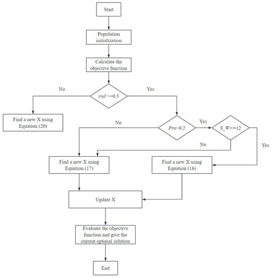
The GOOSE algorithm has two primary stages of development and exploration, through the use of conditions and random variables to achieve balance. The probability of development or exploration is 50%, and the random variable ‘rnd’ is provided. The conditional statement is then used to assign the iteration number evaluation to the development and exploration phases. Furthermore, two new variables are introduced: ‘pro’ and ‘coe’. These variables have random values. Among these, pro is used to verify whether the equation is satisfied. The three variables, ‘pro’, ‘rnd’, and ‘coe’, have values ranging from 0 to 1. Simultaneously, a condition is established to determine if the ‘coe’ value is smaller than 0.17. The value is set to 0.17 when ‘coe’ is less than 0.17.

• Development phase

First, the weight of the stone lifted by the goose is estimated, assuming that its weight is between 5 and 25 g. Equation (8) randomly calculates the weight of the stone in any iteration:

$$S\_W_{it}=randi\left(\left[5,25\right],1,1\right)$$

(8)

Then, using Equation (9), the time from the stone’s release until it contacts the ground is calculated. This time is random, between 1 and the dimension of each iteration cycle.

$$T\_o\_A\_O_{it}=rand\left(1,\dim \right)$$

(9)

Then, when the stone falls to the ground, the goose responsible for guarding emits a scream, and the time from the appearance of the scream to the individual in the goose group is calculated, as shown in Equation (10):

$$T\_o\_A\_S_{it}=rand\left(1,\dim \right)$$

(10)

The total and average sound-propagation times to each goose in the group during the entire iteration process are then calculated using Equations (11) and (12):

$$T\_T={\displaystyle \frac{{\displaystyle \sum \left(T\_o\_A\right)}}{\dim }}$$

(11)

$$T\_A={\displaystyle \frac{T\_T}{\dim }}$$

(12)

Assuming that $pro$ is greater than 0.2 and the stone weight $S\_W_{it}$ is greater than or equal to 12, and in order to protect and awaken the individuals in the geese, the velocity of the falling object is calculated in Equation (13):

$$F\_F\_S=T\_o\_A\_O_{it}\ast {\displaystyle \frac{\sqrt[2]{S\_W_{it}}}{9.81}}$$

(13)

In Equation (14), the distance $D\_S\_T_{it}$ of sound propagation is calculated, where $S\_S$ is the speed of sound propagation in the air.

$$D\_S\_T_{it}=S\_S\ast T\_o\_A\_S_{it}$$

(14)

Next, the distance $D\_G_{it}$ between the guard goose and another goose that is resting or foraging is calculated. Because only the time of sound propagation is required, the result of Equation (15) is multiplied by 0.5, as Equation (15):

$$D\_G_{it}=0.5\ast D\_S\_T_{it}$$

(15)

In order to awaken the individuals in the goose flock, it is necessary to find the best $X_{it}$, that is, to find the best position of the goose, as shown in (16):

$$X_{\left(it+1\right)}=F\_F\_S+D\_G_{it}\ast T\_A^2$$

(16)

If the value of the variable $\mathrm{p}\mathrm{r}\mathrm{o}$ is less than or equal to 0.2 and the stone weight $\mathrm{S}\_{\mathrm{W}}_{\mathrm{i}\mathrm{t}}$ is less than 12, then a new $\mathrm{X}$ calculation is made, as shown in (17):

$$X_{\left(it+1\right)}=F\_F\_S\ast D\_G_{it}\ast T\_A^{2\ast }Coe$$

(17)

Through Equations (13) and (14), the distance of sound propagation and the distance between geese in Equation (17) are obtained. At the same time, a new calculation of the value of the falling speed $F\_F\_S$ of the object is needed, as shown in Equation (18):

$$F\_F\_S=T\_o\_A\_O_{it}\ast {\displaystyle \frac{S\_W_{it}}{9.81}}$$

(18)

As described above, in the development phase, the new $\mathrm{X}$ is calculated by Equations (16) and (17), and the equation used depends on the range of the variable $\mathrm{p}\mathrm{r}\mathrm{o}$ and the stone weight $\mathrm{S}\_{\mathrm{W}}_{\mathrm{i}\mathrm{t}}$.

2.

Exploration stage

The goose that is resting or foraging awakens at the optimal location during the exploration phase. It continues calling to alert the other geese in the flock. Use Equations (10) and (11) to determine whether the value of the minimum time $Min\_T$ is larger than the total time $T\_T$ if the value of the variable $rnd$ is less than 0.5. If it is, set the minimum time $Min\_T$ to equal the entire time $T\_T$.

The variable alpha is defined, and its value range is 0~2, and it decreases linearly towards zero as the iterations proceed. Equation (19) is used to improve the results of new $X$ in the search space.

$$alpha=\left(2-\left({\displaystyle \frac{loop}{\frac{Max\_It}{2}}}\right)\right)$$

(19)

$Max\_It$ is the maximum number of iterations. In order to turn the search phase to the direction of the answer that is most likely to be the optimal solution, it is necessary to calculate the values of $Min\_T$ and alpha.

$Min\_T$ and alpha are utilized to enhance GOOSE’s search capability by ensuring that it randomly examines other individuals in the search space using $\mathrm{r}\mathrm{a}\mathrm{n}\mathrm{d}\mathrm{n}(1,\mathrm{d}\mathrm{i}\mathrm{m})$. Equation (20) illustrates how the smallest value of the time is multiplied by the alpha and the random number, then added to the optimal location in the search space:

$$\begin{array}{l}{X}_{\left(it+1\right)}=randn\left(1,\dim \right)\ast \left(Min\_T\ast alpha\right)\\ \hspace{1em}+Best\_pos\end{array}$$

(20)

In the equation, we find the number of dimensions of the $\mathrm{d}\mathrm{i}\mathrm{m}$ problem and $\mathrm{B}\mathrm{e}\mathrm{s}\mathrm{t}\_\mathrm{p}\mathrm{o}\mathrm{s}$ is the best position to find in the search space.

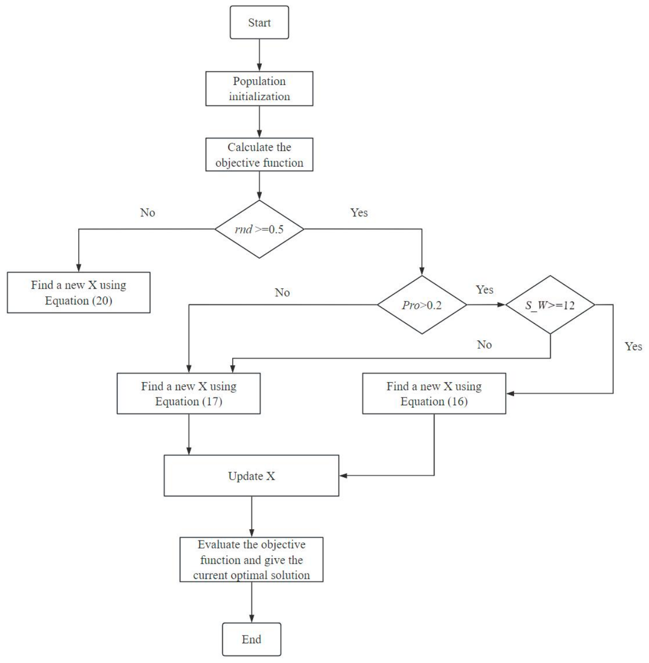
In summary, the GOOSE algorithm begins by randomly generating a population. In the first iteration, it checks the values in the population to restore the values outside the boundary, and performs the objective function to determine the best position and optimal solution within the search boundary. In this algorithm, a total of three methods are used to find new X in the search space, namely, the development phase of Equations (16) and (17) and the search phase of Equation (20). The specific process of the algorithm is shown in Figure 1:

Figure 1. Algorithm single optimization process.

2.3. Permutation Entropy

Bandt and Pompe [23] proposed the concept of permutation entropy (PE) in 2002. Because PE has strong noise resistance and rapid computation, it has been widely used in the field of mechanical fault diagnosis. The specific calculation process is as follows:

Assuming the time series ${\mathrm{X}}_{\mathrm{i}}=\left\{{\mathrm{x}}_1,{\mathrm{x}}_2,{\mathrm{x}}_3,\cdots ,{\mathrm{x}}_{\mathrm{N}},\right\}$ with length N, and given the embedding dimension $\mathrm{m}$ and the delay time $\mathrm{t}$, the phase space reconstruction of the time series is carried out by using the spatial delay coordinates, as shown in Equation (21):

$$Y=\left[\begin{array}{cccc}x\left(1\right)& x\left(1+t\right)& \dots & x\left(1+\left(m-1\right)\lambda \right)\\ x\left(2\right)& x\left(2+t\right)& \dots & x\left(2+\left(m-1\right)\lambda \right)\\ ⋮& ⋮& & ⋮\\ x\left(j\right)& x\left(j+t\right)& \dots & x\left(j+\left(m-1\right)\lambda \right)\\ ⋮& ⋮& & ⋮\\ x\left(K\right)& x\left(K+1\right)& \dots & x\left(K+\left(m-1\right)\lambda \right)\end{array}\right]$$

(21)

Among these, there are a total of $\mathrm{K}$ reconstruction vectors, $\mathrm{K}=\mathrm{N}-(\mathrm{m}-1)$. Each reconstruction vector is sorted in ascending order to obtain the index sequence $\mathrm{S}\left(\mathrm{l}\right)$, as shown in Equation (22):

$$\begin{array}{l}S\left(l\right)=\left\{j_1,j_2,\cdots ,j_m\right\},l=1,2,\cdots ,K\\ \left(K\le m!\right)\end{array}$$

(22)

The m-dimensional vector may have $\mathrm{m}!$ sorting methods. The permutation entropy of time series $\mathrm{X}$ is calculated from the probability of occurrence of various situations $\left\{{\mathrm{P}}_1,{\mathrm{P}}_2,{\mathrm{P}}_3,\cdots ,{\mathrm{P}}_{\mathrm{k}},\right\}$. The permutation entropy value of time series X is

$$H_{pe}=-{\displaystyle \sum _{i=1}^k{P}_i\ln P_i}$$

(23)

The maximum value of permutation entropy is $\mathrm{l}\mathrm{n}(\mathrm{m}!)$. By normalizing Equation (23), we can get

$$0\le H_{PE}={\displaystyle \frac{H_{pe}}{\ln \left(m!\right)}}\le 1$$

(24)

The level of chaos in the time series can be inferred from the permutation entropy alone. It can more accurately depict the current status of the time series after normalization. The more complex and disorganized the time series, the higher the entropy value; on the other hand, the more regular and periodic the time series, the lower the entropy value.

Throughout this work the embedding dimension is 5 and the delay is one sample. The criterion is computed for each mode separately, and the value taken as the fitness of a candidate pair (K, α) is the smallest of the entropies of the modes obtained with that pair; the same convention is applied to the sample, information and envelope entropies.

2.4. Generalized Morse and Element Analysis

The generalized Morse wavelet is a family of analytic wavelets defined by two parameters. It can encompass other commonly used analytical wavelets within a unified family, and it has no negative-frequency components. It provides high time–frequency resolution [28]. Furthermore, the frequency-domain form of the Morse wavelet is relatively simple, which facilitates the derivation of important analytical equations.

As shown in Equation (25), the generalized Morse wavelet is denoted by ${\mathsf{\psi }}_{\mathsf{\beta },\mathsf{\gamma }}\left(\mathrm{t}\right)$, which is defined in the frequency domain of $\mathsf{\beta }\ge 0$ and $\mathsf{\gamma }\ge 0$ as

$${\psi }_{\beta ,\gamma }\left(t\right)={\displaystyle \frac{1}{2\pi }}\cdot {\int }_{-\infty }^{\infty }{\psi }_{\beta ,\gamma }\left(\omega \right)e^{i\omega t}d\omega$$

(25)

$${\psi }_{\beta ,\gamma }\left(\omega \right)\equiv a_{\beta ,\gamma }\cdot {\omega }^{\beta }\cdot e^{-{\omega }^{\gamma }}\cdot \left\{\begin{array}{ll}1& \omega >0\\ {\displaystyle \frac{1}{2}}& \omega =0\\ 0& \omega <0\end{array}\right.$$

(26)

The equation involves $e$, the Euler number, $e\approx 2.71828$, ${\alpha }_{\beta ,\gamma }$ as the real normalized constant, $\omega$ as the angular frequency or radian frequency, $\gamma$ as the high-frequency signal attenuation in the wavelet time-domain, and $\beta$ as the low-frequency signal waveform.

Element analysis is a signal analysis and processing method with strong adaptability [29]. In order to deduce the characteristics of the original signal, this approach evaluates the accuracy of the extracted signal from the magnitude of white noise or power-law noise. It then eliminates the noisy signal that influences the diagnostic result.

An isolated and time-localized “event” in the gathered signals is analysed via element analysis, which is based on the generalized Morse wavelet and continuous wavelet transform. A time series model, called the element model, is presented to capture the signals made up of these distinct and comparable “events” [30]:

$$x\left(t\right)={\displaystyle \sum _{n=1}^{N}R}\left\{c_n{\psi }_{\mu ,\gamma }\left({\displaystyle \frac{t-t_n}{{\rho }_n}}\right)\right\}+x_{\epsilon }\left(t\right)$$

(27)

The equation involves the following: $\mathrm{x}\left(\mathrm{t}\right)$ is a real-valued time series; $\mathsf{\psi }\left(\mathrm{t}\right)$ is a complex-valued function that includes phase shift, rescaling, and time offset; $\mathrm{R}\{·\}$ is the real component; amplitude, time position, and scale of time are represented by ${\mathrm{c}}_{\mathrm{n}},{\mathrm{t}}_{\mathrm{n}},{\mathsf{\rho }}_{\mathrm{n}}$, respectively; and Gaussian noise is represented by ${\mathrm{x}}_{\mathsf{ϵ}}\left(\mathrm{t}\right)$. μ and γ determine the features of the element function ${\mathsf{\psi }}_{\mathsf{\mu },\mathsf{\gamma }}\left(\mathrm{t}\right)$.

By using the Morse wavelet containing parameters $\beta$ and $\gamma$ to transform the equation $x\left(t\right)$, we can obtain

$$\begin{array}{l}{w}_{\beta ,\gamma }\left(\tau ,s\right)={\displaystyle \frac{1}{2}}{\displaystyle {\displaystyle \sum _{n=1}^N}{c}_n}{\displaystyle {\int }_{-\infty }^{\infty }\frac{1}{s}}{\psi }_{\beta ,\gamma }^{\ast }\left({\displaystyle \frac{t-\tau }{s}}\right){\psi }_{\mu ,\gamma }\left({\displaystyle \frac{t-t_n}{{\rho }_n}}\right)dt\\ +{\epsilon }_{\beta ,\gamma }\left(\tau ,s\right)\end{array}$$

(28)

The wavelet transform of noise $x_{ϵ}\left(t\right)$ is represented by the equation ${\epsilon }_{\beta ,\gamma }(\tau ,s)$. The time-scale position $(\widehat{\tau },\widehat{s})$ is the maximum point of the transform. The wavelet transform modulus achieves a local maximum at this point in the following manner:

$${\displaystyle \frac{\partial }{\partial \tau }}\left|{\omega }_{\beta ,\gamma }\left(\tau ,s\right)\right|={\displaystyle \frac{\partial }{\partial s}}\left|{\omega }_{\beta ,\gamma }\left(\tau ,s\right)\right|=0$$

(29)

$${\displaystyle \frac{{\partial }^2}{\partial s^2}}\left|{\omega }_{\beta ,\gamma }\left(\tau ,s\right)\right|<0$$

(30)

$${\displaystyle \frac{{\partial }^2}{{\partial \tau }^2}}\left|{\omega }_{\beta ,\gamma }\left(\tau ,s\right)\right|<0$$

(31)

In the same γ family, the β-order Morse wavelet transform of the function ${\mathsf{\psi }}_{\mathsf{\mu },\mathsf{\gamma }}(\mathrm{t}/\mathsf{\rho })$ is expressed as

$${\displaystyle {\int }_{-\infty }^{\infty }\frac{1}{s}}{\psi }_{\beta ,\gamma }^{\ast }\left({\displaystyle \frac{t-\tau }{s}}\right){\psi }_{\mu ,\gamma }\left({\displaystyle \frac{t}{\rho }}\right)dt={\xi }_{\beta ,\mu ,\gamma }\left({\displaystyle \frac{\tau }{\rho }},{\displaystyle \frac{s}{\rho }}\right)$$

(32)

In the equation, ${\xi }_{\beta ,\mu ,\gamma }\left(\tau ,s\right)$ is a modified wavelet function, defined as follows:

$${\xi }_{\beta ,\mu ,\gamma }\left(\tau ,s\right)\equiv {\displaystyle \frac{e_{\beta ,\gamma }{e}_{\mu ,\gamma }}{e_{\beta +\mu ,\gamma }}}{\displaystyle \frac{s^{\beta }}{{\left(\sqrt[\gamma ]{s^{\gamma }+1}\right)}^{\beta +\mu +1}}}{\psi }_{\beta +\mu ,\gamma }\left({\displaystyle \frac{\tau }{\sqrt[\gamma ]{s^{\gamma }+1}}}\right)$$

(33)

Equation (32) shows that when the Morse function ${\mathsf{\psi }}_{\mathsf{\mu },\mathsf{\gamma }}(\mathrm{t}/\mathsf{\rho })$ is wavelet transformed, the time and scale of the original function ${\psi }_{\mu ,\gamma }\left(t\right)$ change, whereas the amplitude remains unchanged.

A wavelet of order $(\mathsf{\beta }+\mathsf{\mu })$ appears in Equation (33). $\mathsf{\mu }$ and $\mathsf{\beta }$ correspond to the power of ω in the frequency domain, which is the multiplication operation in the frequency corresponding to the wavelet transform, so they can be merged.

Equation (33) can determine the values of the wavelet transform at the maximum point, which are related to the attributes of the signal elements. According to ${\xi }_{\beta ,\mu ,\gamma }\left(\tau ,s\right)$, we can get

$$\begin{array}{l}{w}_{\beta ,\gamma }\left(\tau ,s\right)={\displaystyle \frac{1}{2}}{\displaystyle \sum _{n=1}^N{c}_n}{\xi }_{\beta ,\mu ,\gamma }\left({\displaystyle \frac{\tau -t_n}{{\rho }_n}},{\displaystyle \frac{s}{{\rho }_n}}\right)\\ +{\epsilon }_{\beta ,\gamma }\left(\tau ,s\right)\end{array}$$

(34)

Then, the expected value of the square norm in the wavelet transform is obtained by the approximate calculation of Equation (35):

$$\begin{array}{l}E\left\{{\left|{\omega }_{\beta ,\gamma }\left(\tau ,s\right)\right|}^2\right\}\approx {\displaystyle \frac{1}{4}}{{\displaystyle \sum _{n=1}^N{\left|c_n\right|}^2\left|{\xi }_{\beta ,\mu ,\gamma }\left(\frac{\tau -t_n}{{\rho }_n},\frac{s}{{\rho }_n}\right)\right|}}^2\\ +E\left\{{\left|{\epsilon }_{\beta ,\gamma }\left(\tau ,s\right)\right|}^2\right\}\end{array}$$

(35)

The interactions among several terms are neglected in Equation (35). The cross term between the wavelet transform and the element function’s noise can be disregarded under the zero-mean assumption. In a particular time-scale, Equation (35) can yield a good approximation close to the maximum value of each transformation, provided that sufficient intervals exist between events.

The identification of the maxima follows from the element model rather than from a separate statistical test. For an element function that decays monotonically away from its maximum, each event contributes exactly one transform maximum; the modulus of the wavelet transform of the reconstructed signal therefore contains one maximum per impact, and because the impacts are similarly shaped these maxima all occur at the same transformation period, so that they form a single horizontal line in the time–scale map. Two circumstances can nevertheless give rise to spurious maxima: the interaction between events, which is neglected in the derivation of Equation (35), and a non-monotonic decay of the wavelet modulus, which occurs for extreme choices of γ and β. Such spurious maxima lie below the noise level and are removed by an amplitude cut-off set at that level, which Equation (35) provides as the expected squared modulus of the transform of the background noise. The influence region of the element model is used only to attribute each surviving maximum to the time–scale region of a single event, so that one impact is not counted more than once; it is not used as a further acceptance criterion, and no significance test in the sense of ref. [30] is applied. The period is then taken as the mean spacing of the surviving maxima along the time axis.

After derivation, the maximum value of the Morse wavelet transform of Morse function ${\psi }_{\mu ,\gamma }(t/\rho )$ can be obtained:

$${\xi }_{\beta ,\mu ,\gamma }^{\max }={\displaystyle \frac{e_{\beta ,\gamma }{e}_{\mu ,\gamma }}{2\pi \gamma }}\Gamma \left({\displaystyle \frac{\beta +\mu +1}{\gamma }}\right)v_{\beta ,\mu ,\gamma }$$

(36)

We use ${\psi }_{\mu ,\gamma }(t/\rho )$ to correct ${\psi }_{\beta ,\gamma }\left(t\right)$, and use the transformation maximum point (τ Ω, s Ω) to estimate the element attributes $c_n,t_n$ and ${\rho }_n$. Taking ${\widehat{\omega }}_n={\omega }_{\beta ,\gamma }(\widehat{\tau },\widehat{s})$ as the observed maximum value of the Nth wavelet transform, we have

$${\stackrel{\wedge }{t}}_n={\stackrel{\wedge }{\tau }}_n$$

(37)

$${\stackrel{\wedge }{\rho }}_n={\displaystyle \frac{{\stackrel{\wedge }{s}}_n}{{\stackrel{\sim }{s}}_{\beta ,\mu ,\gamma }^{\max }}}$$

(38)

$${\stackrel{\wedge }{c}}_n={\displaystyle \frac{{\stackrel{\wedge }{w}}_n}{{\xi }_{\beta ,\mu ,\gamma }^{\max }}}$$

(39)

$${\omega }_{{\stackrel{\wedge }{\rho }}_n}={\omega }_{{\stackrel{\wedge }{s}}_n}{\displaystyle \frac{{\omega }_{\mu ,\gamma }}{{\omega }_{\beta ,\gamma }}}{\stackrel{\sim }{s}}_{\beta ,\mu ,\gamma }^{\max }={\omega }_{{\stackrel{\wedge }{s}}_n}{\displaystyle \frac{{\omega }_{\mu ,\gamma }}{{\omega }_{\beta ,\gamma }}}{\left({\displaystyle \frac{\beta }{\mu +1}}\right)}^{1/\gamma }$$

(40)

Equation (40) describes the relationship between the frequency of the Nth wavelet transform maximum and the frequency of the corresponding element function.

To summarize, the fundamental concept of the element analysis algorithm involves utilizing the local maximum of the wavelet transform to approximate the complex value coefficient $c_n$, the event scale ${\rho }_n$, and the event location $t_n$ in Equations (37)–(39). To recreate the source signal, the collected parameters are then entered into Equation (27).

3. Rolling Bearing Fault Diagnosis Method

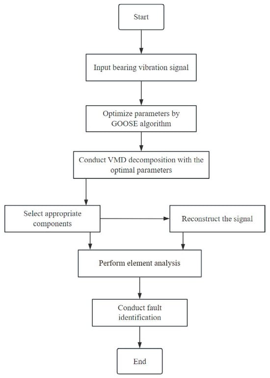
The element analysis method has a good effect on the analysis of the regular impact signal in the vibration signal, and the optimal component contains substantial rolling bearing fault information after the VMD parameters are optimized by the GOOSE algorithm with permutation entropy as the objective function. Thus, to diagnose rolling bearing faults, this research integrates element analysis with the GOOSE-VMD rolling bearing defect feature information extraction approach. The specific steps are as follows:

• Input the bearing vibration signal to determine its relevant parameters, such as sampling rate, sampling time, etc.
• The initial parameters of GOOSE are set, and the algorithm is used to optimize the number of VMD mode decomposition K and the penalty factor α. The final optimization result is output, and the vibration signal is decomposed by using the parameter combination.
• The excess kurtosis and the correlation coefficient are computed for every mode. A mode is admitted as a candidate only if its excess kurtosis exceeds three, which is the condition for the component to be distinctly impulsive; among the candidates the two with the largest correlation coefficients are retained, and the signal is reconstructed from them. The kurtosis referred to throughout is the excess kurtosis, that is, the kurtosis minus three, so that a value of zero corresponds to a Gaussian distribution.
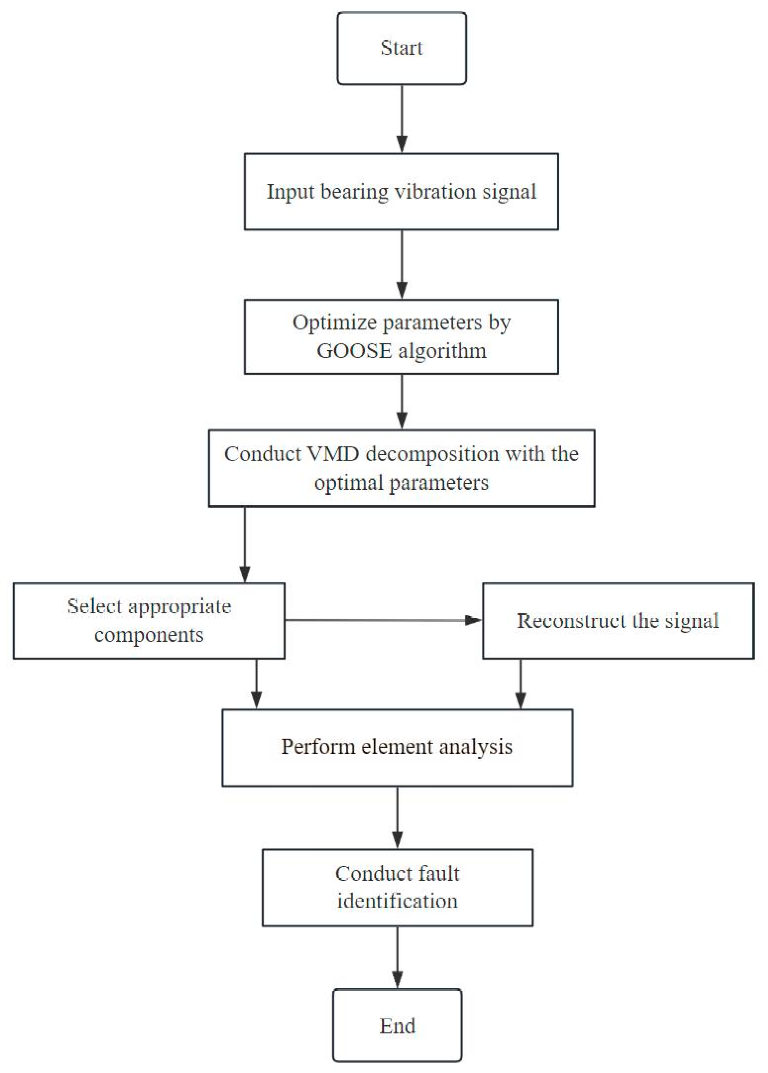
• The element analysis method is used to analyse the selected components and reconstructed signals, and the frequency of the maximum point of the transformation is calculated. The fault type of the bearing is comprehensively judged against the theoretical fault frequency of the faulty bearing. The specific process is shown in Figure 2:
  

  Figure 2. Fault diagnosis process of rolling bearings based on GOOSE-VMD and element analysis.

4. Rolling Bearing Fault Diagnosis Experiment

4.1. Comparative Validation of Effectiveness

In order to verify the effectiveness of the proposed method, a simulated signal of a rolling bearing with an outer-ring fault is constructed, as in Equation (41):

$$x\left(t\right)=A{e}^{-2\pi gft}\mathrm{s}\mathrm{i}\mathrm{n}\left(2\pi ft\sqrt{1-g^2}\right)$$

(41)

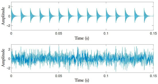
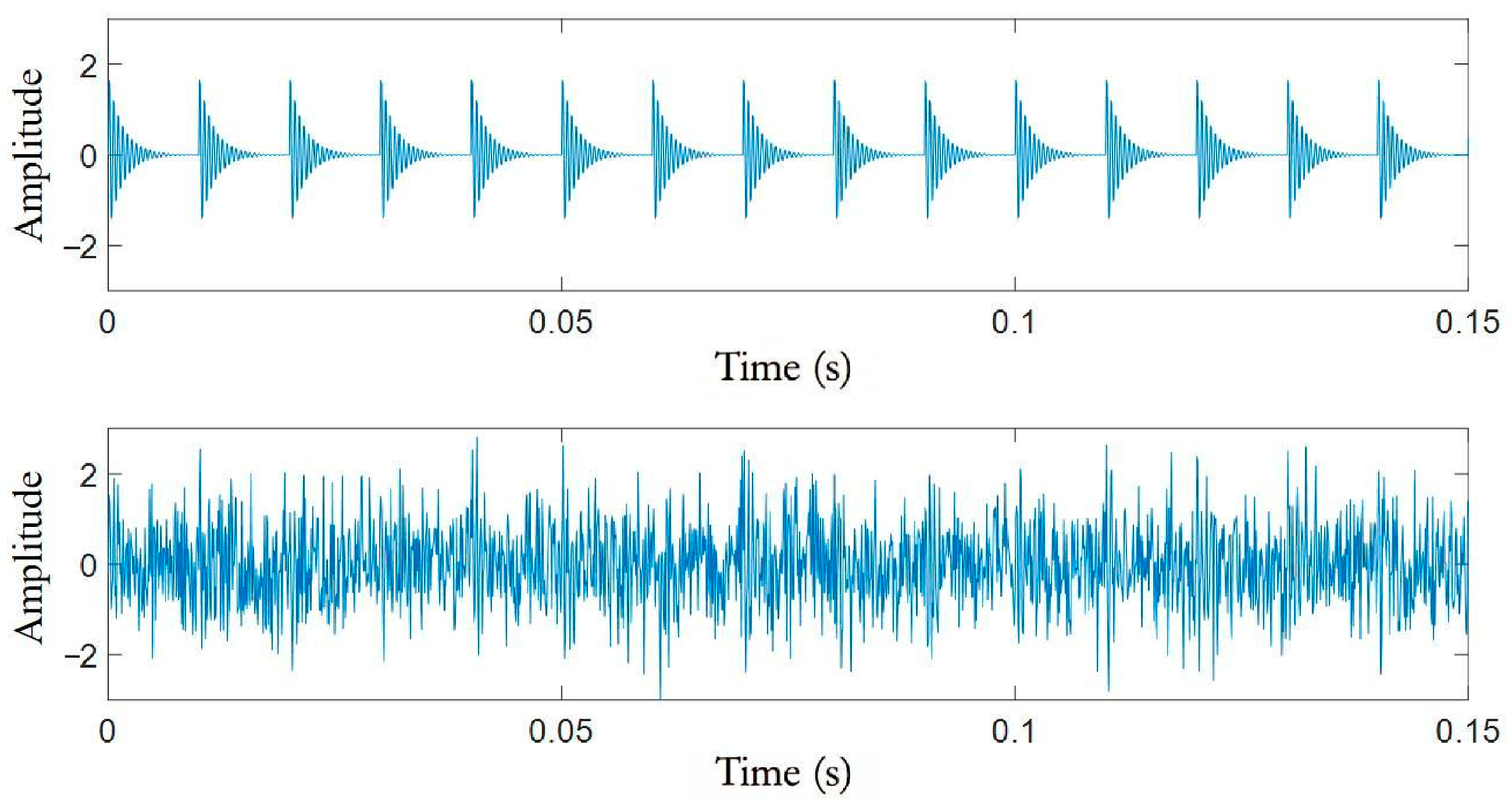
The displacement constant $A$ in the equation has a value of 2, the damping coefficient g has a value of 0.05, the natural frequency $f$ has a value of 2000 Hz, the sampling frequency (12,000 Hz), the fault time (0.01 s), and there are 2048 sampling points. Gaussian white noise with a signal-to-noise ratio of −6 dB is introduced to the simulation signal in order to replicate the real scenario when gathering the rolling bearing vibration signal. Figure 3 displays the time-domain waveform of the signal’s first 0.15 s.

Figure 3. Time-domain waveform diagram of simulated signal.

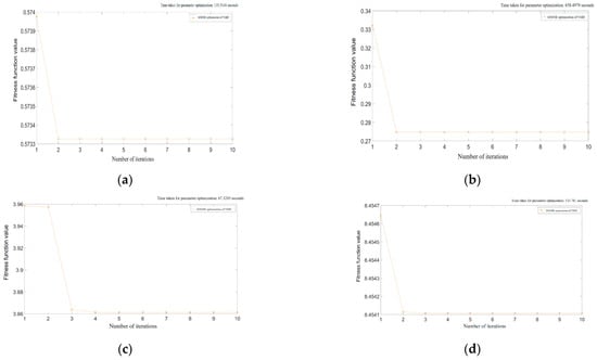
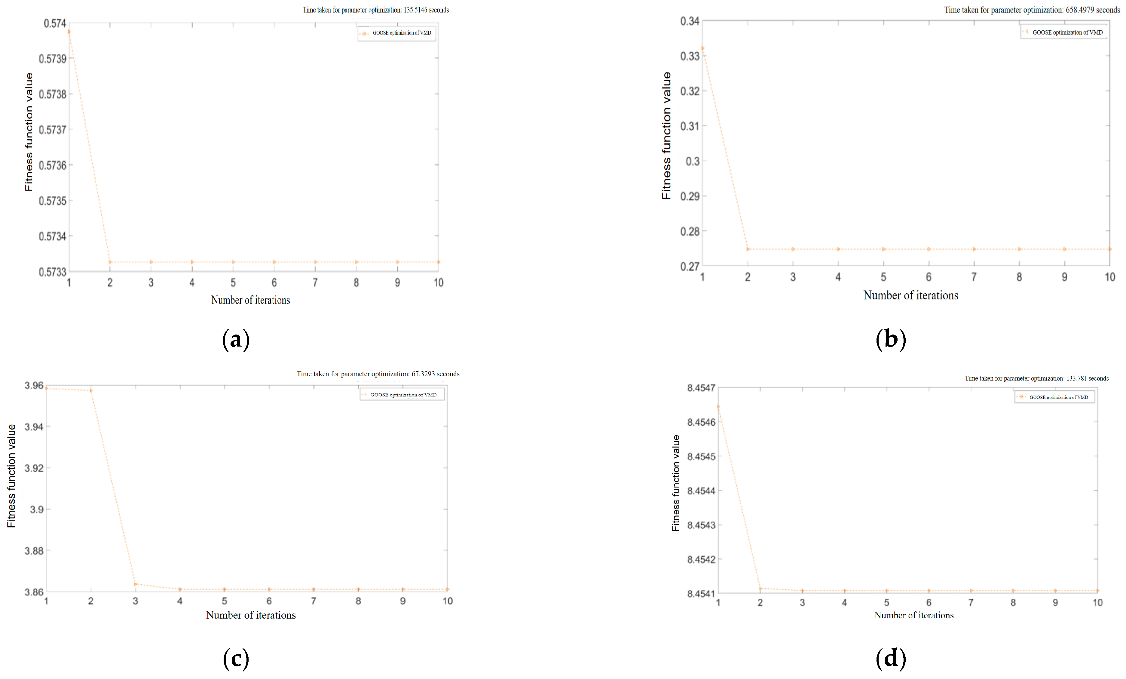
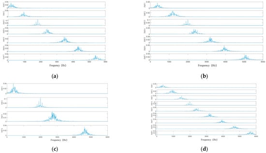
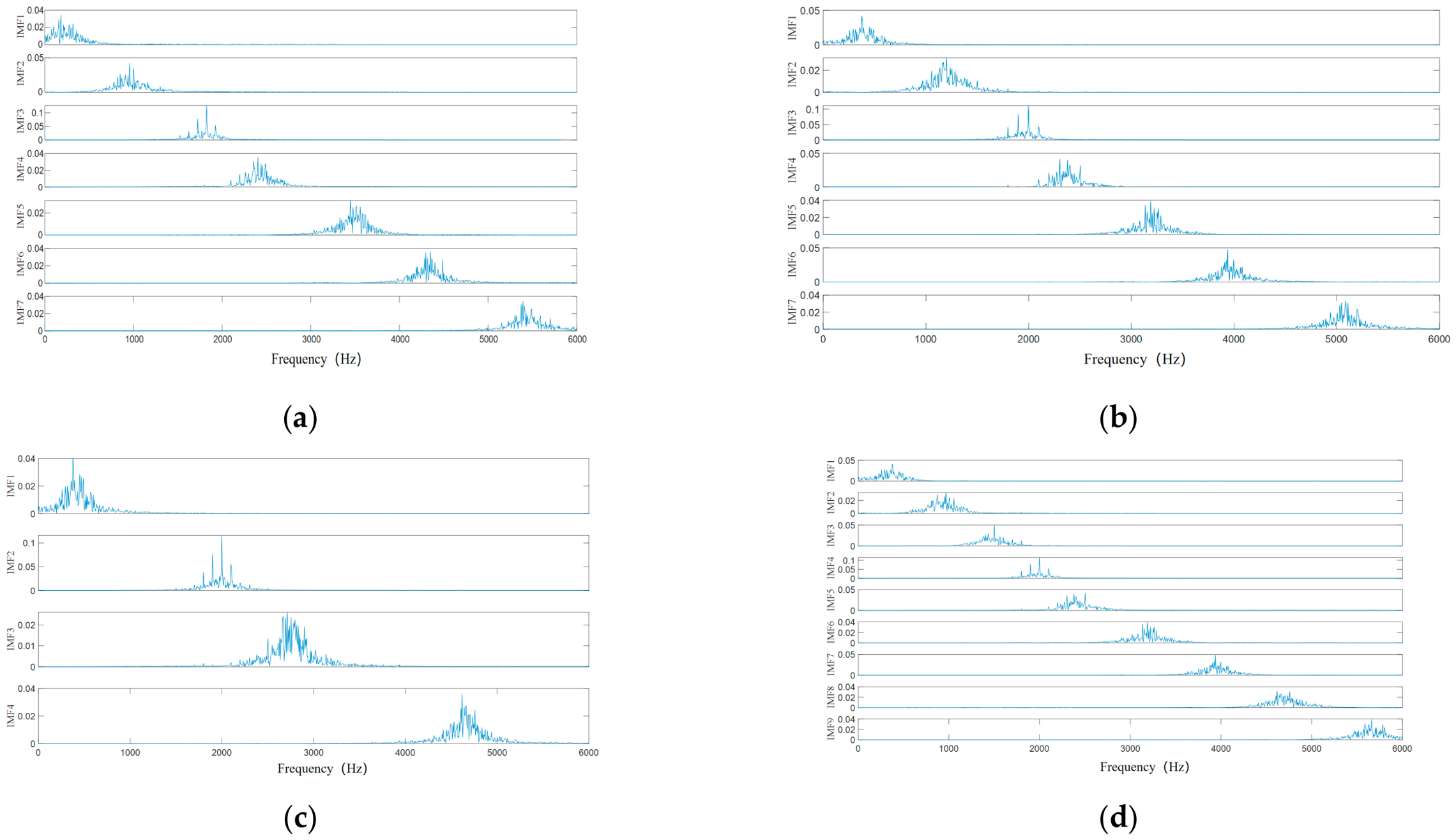
Figure 4 and Figure 5 illustrate how the GOOSE algorithm uses the permutation, sample, information, and envelope entropies as objective functions to optimize the VMD parameters and decompose the simulation signal after the initial parameters are determined. The fitness values of the four criteria are not directly comparable, as they have different ranges and units: the permutation entropy used here is confined to the interval [0, 1], whereas the information and envelope entropies take values near 3.9 and 8.45, respectively. The four criteria are therefore compared through the decomposition they produce (Figure 5) and through the computation time, not through their fitness values. Over the ten iterations used, none of the four criteria improves substantially after the first iteration or two. For the permutation and envelope entropies the total change over the whole run is only 7 × 10⁻⁴ and 6 × 10⁻⁴, respectively, and in both cases the change occurs almost entirely between the first and second iterations; the curves are then flat. This indicates that these two criteria vary little with K and α over the search range used, so that the fitness landscape is nearly flat with respect to them, rather than that the optimizer converges particularly quickly. A flat fitness landscape has a practical consequence: for these criteria the decomposition quality is insensitive to K and α over a wide range, so the optimizer mainly removes the need to search that range by hand rather than lifting the quality above what a well-chosen fixed pair would give. The value of the optimization lies in consistency across records of different signal-to-noise ratios, not in a large improvement of the fitness value itself. Permutation entropy is adopted as the objective function because it measures the sequential ordering of neighbouring samples directly and is therefore the criterion most closely related to the periodic impulses produced by a bearing defect, and because the decomposition it produces separates the fault-related frequency components most clearly (Figure 5). Its optimization time of 135.5 s is second only to that of the sample entropy (658.5 s) among the four criteria, the envelope entropy being marginally faster at 133.8 s and the information entropy being the fastest of them all at 67.3 s. Consequently, permutation entropy is not selected for its speed.

Figure 4. Parameter optimization iteration diagram over ten iterations for the four entropy criteria: (a) permutation entropy (135.5 s); (b) sample entropy (658.5 s); (c) information entropy (67.3 s); (d) envelope entropy (133.8 s).

Figure 5. IMF spectra of VMD under four entropy optimization criteria. (a) Permutation entropy; (b) sample entropy; (c) information entropy; (d) envelope entropy.

Figure 4 and Figure 5 show that no obvious aliasing occurs in the IMF components after decomposition.

The components used for element analysis are selected from the decomposed IMFs, which carry different amounts of fault information and noise. Kurtosis and the correlation coefficient are the two indicators commonly used for this purpose: the first measures how impulsive a component is, and the second how much of the original signal it retains. A component is therefore admitted as a candidate only if its excess kurtosis exceeds three, and among the candidates the two with the largest correlation coefficients are retained for reconstruction. The indicators for each component are listed in Table 1:

Table 1. Excess kurtosis and correlation coefficient of each mode of the simulated signal.

	IMF 1	IMF2	IMF3	IMF4	IMF5	IMF6	IMF7
Kurtosis	0.2839	3.4543	3.3469	3.0127	2.9040	2.9629	2.8931
Correlation Coefficient	0.3164	0.3691	0.5259	0.3405	0.3164	0.2999	0.3097

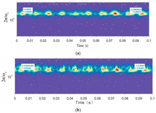
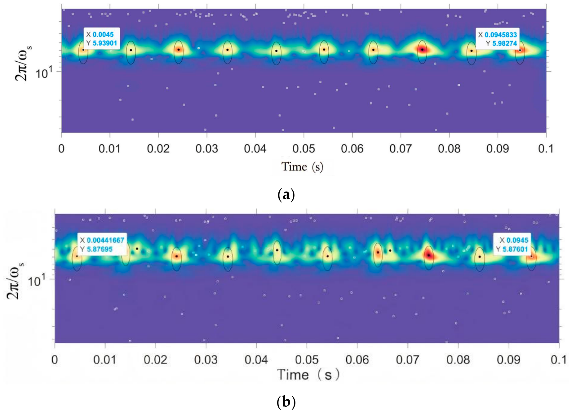
Applying this criterion to the data of Table 1 retains IMF2 and IMF3, and these two components are used to reconstruct the signal for the element analysis. Figure 6 displays the findings. The element analysis was carried out with γ = 10, β = 10 and μ = 2. The transform is evaluated over a fixed range of scales chosen to bracket the duration of the impact events. In the time–scale map of Figure 6, the maxima of the impact train lie at a transformation period 2π/ω_s of about 5, and the range covered extends beyond this towards longer periods.

Figure 6. Analysis of simulated signal components and their reconstructed signal elements. (a) IMF2 element analysis and (b) reconstructed signal element analysis.

The black dots in Figure 6 represent the maximum points of the wavelet transform for impact events, or the signal impacts caused by bearing faults. The abscissa represents time, and the ordinate represents the transformation period. The dispersed white boxes represent other transform maxima unrelated to the impact information, and the area encircled by the black line around the black dot is the influence area of the central maximum point (the gathering area of the maximum point of the noise transform closely related to the impact event). Table 2 presents the calculation and comparison of the greatest point of transformation in the diagram’s period and frequency with the theoretical data of the faulty bearing simulation signal.

Table 2. Analysis results of IMF2 and reconstructed signal elements.

	Element Analysis Results		Theoretical Data of Simulated Signals
	Cycle (s)	Frequency (Hz)	Cycle (s)	Frequency (Hz)
IMF2	0.01001	99.90	0.01	100
Reconstructed signal	0.01001	99.90

An outer-ring fault can be diagnosed by comparing the element analysis results in Table 2 and the theoretical data of the outer-ring fault simulation signal. This comparison reveals that the maximum point of the IMF2 component and the reconstructed signal have periods and frequencies that are extremely similar to the theoretical outer ring fault period and frequency of the simulation signal.

The GOOSE algorithm was run with a population of fifteen individuals and a maximum of ten iterations. The settings common to all the cases analysed, including the search intervals of K and α, are collected in Table 3. The parameters returned by the optimizer were K = 7 and α = 5307 for the permutation entropy, K = 7 and α = 5077 for the sample entropy, K = 4 and α = 5422 for the information entropy, and K = 9 and α = 3476 for the envelope entropy.

Table 3. Settings common to all the cases analysed.

GOOSE Population	GOOSE Iterations	Search Range of K	Search Range of α	Fault-Frequency Tolerance
15	10 (simulated signal) 15 (experimental records)	[3, 10]	[50, 5500]	±3 Hz

4.2. Fault Diagnosis Example of Faulty Rolling Bearing

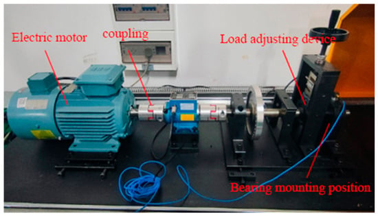
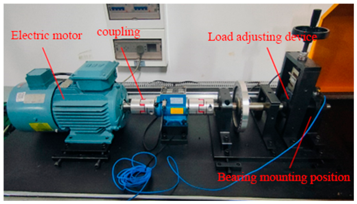
This section describes an experimental fault diagnosis experiment, constructed to collect vibration data from the faulty rolling bearing. The method described in this research is used for feature extraction and fault type diagnosis. The experimental apparatus is shown in Figure 7:

Figure 7. Bearing testing experimental platform.

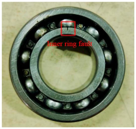
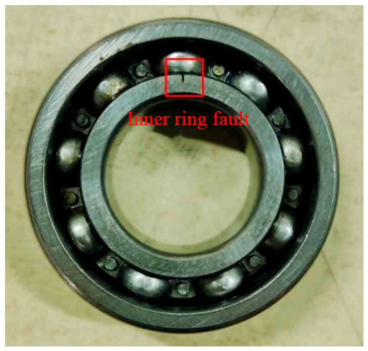
The test rig consists of a three-phase electric motor, a flexible coupling, a bearing mounting and load-adjusting device, an accelerometer and a data-acquisition system; the accelerometer is mounted radially on the bearing housing, directly above the bearing under test. The bearing tested on the platform is an NSK6205 bearing, as shown in Figure 8 and Table 4; the defect is a narrow radial slot cut into the inner-race surface, with a width of the order of 0.3 mm:

Figure 8. The NSK 6205 bearing used in the test, with a simulated inner-ring fault; the defective region is marked by the red rectangle.

Table 4. Main parameters of rolling bearing NSK6205.

External Diameter	Internal Diameter	Pitch Diameter	Width	Number of Ball Bearings	Ball Diameter	Contact Angle
52 mm	25 mm	39.04 mm	15 mm	9	7.94 mm	0°

According to the parameters in Table 4, the inner-ring fault frequency of the bearing can be calculated using Equation (42):

$$f_{bi}={\displaystyle \frac{Z}{2}}·\left(1+{\displaystyle \frac{d}{D}}cos\alpha \right)·f_r$$

(42)

In the equation, f_bi is the inner-ring fault frequency, Z is the number of balls, d is the ball diameter, D is the pitch diameter, α is the contact angle, and f_r is the spindle rotation frequency.

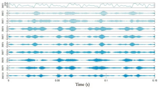
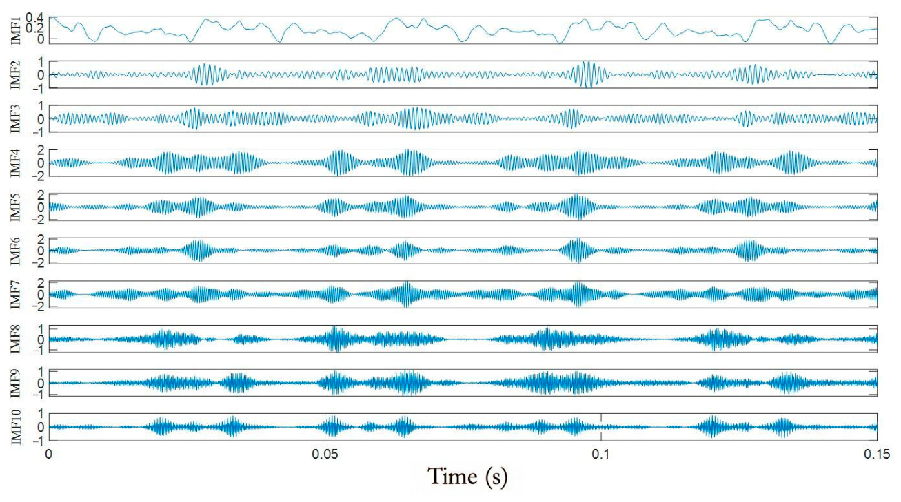
During the experiment, the speed was set to 1800 rpm and the signal was recorded for 60 s at a sampling frequency of 10,240 Hz, after the rotation had stabilized; for the inner-ring test reported here, no radial load was applied. The segment analysed is a 0.15 s (1536-sample) excerpt of that record, and the element analysis is carried out on 0.05 s of it. Using permutation entropy as the objective function for parameter optimization—with a population of fifteen individuals and a maximum of fifteen iterations—the decomposed IMF components are shown in Figure 9:

Figure 9. Time-domain waveforms of the ten IMF components obtained by GOOSE-VMD from the measured inner-ring fault signal.

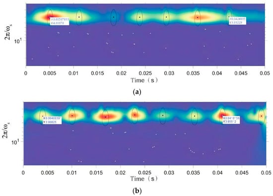
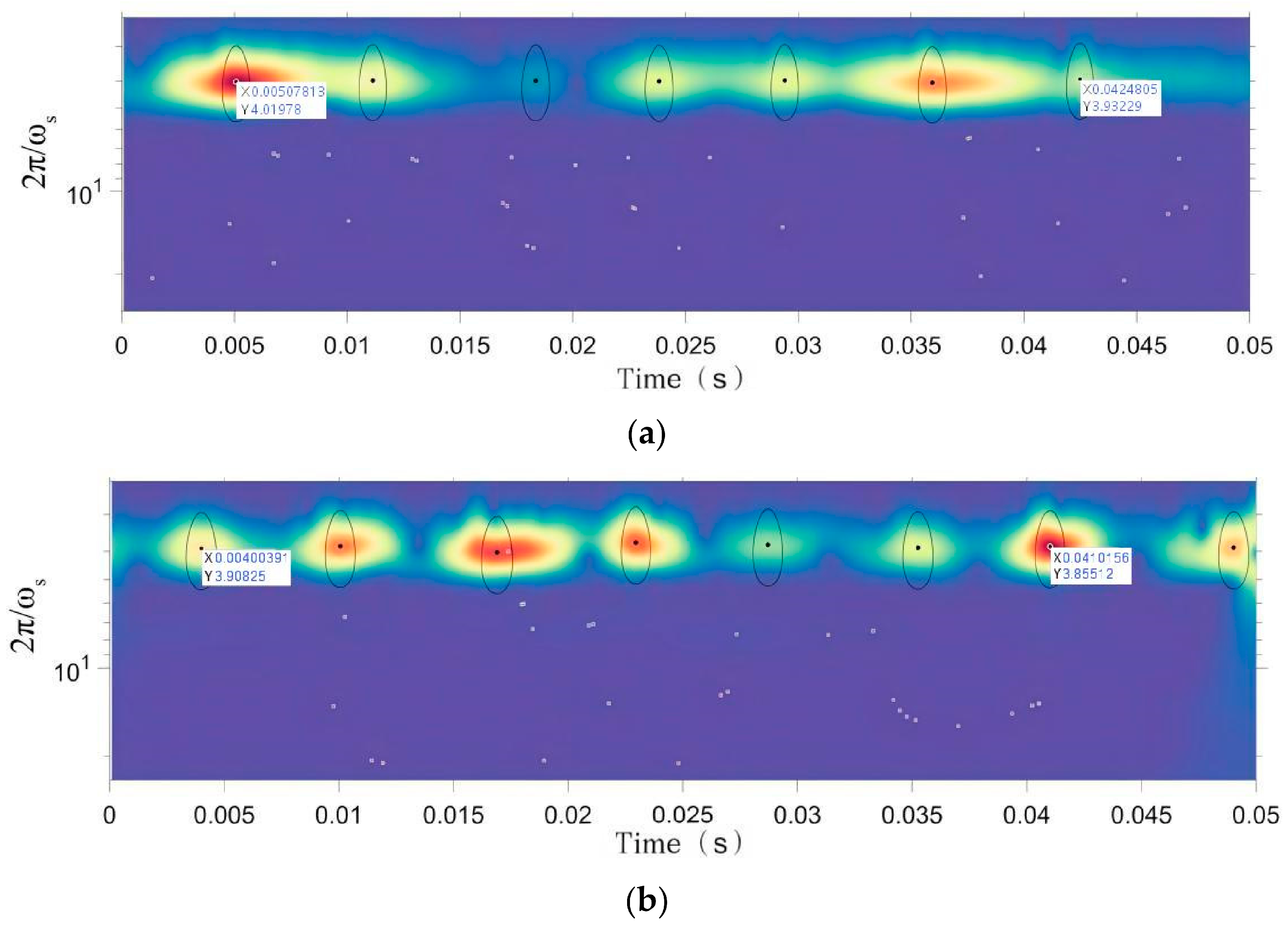
The kurtosis and the correlation coefficients were calculated for all IMF components and these are listed in Table 5. The two components with the highest correlation coefficients among those with an excess kurtosis above 3—IMF3 (3.4110, 0.4291) and IMF4 (3.3989, 0.4381)—were retained and used to reconstruct the signal. The element analysis was then applied to the reconstructed signal, which carries both retained components, and to IMF3. The optimizer returned K = 10 and α = 3706 for this case, and the element analysis was carried out with γ = 3, β = 20 and μ = 6. The same range of transformation periods was used, and the impact maxima in the map of Figure 10 again lie at 2π/ω_s of about 5. Signal reconstruction and element analysis were performed, and the results are shown in Figure 10:

Table 5. Excess kurtosis and correlation coefficient of the modes of the measured inner-ring fault signal (K = 10).

	IMF1	IMF2	IMF3	IMF4	IMF5	IMF6	IMF7	IMF8	IMF9	IMF10
Kurtosis	5.6639	4.9588	3.4110	3.3989	3.4292	3.5199	2.9653	2.7661	4.3172	3.8765
Correlation Coefficient	0.2129	0.3615	0.4291	0.4381	0.4039	0.4146	0.4621	0.3046	0.2845	0.1315

Figure 10. Element analysis of the inner-ring fault signal: (a) IMF3 and (b) reconstructed signal.

The period and frequency of the maximum transformation point in the graph were calculated and compared with the theoretical data of the inner-ring faulty bearing, as shown in Table 6:

Table 6. Analysis results of IMF3 and reconstructed signal elements.

	Element Analysis Results		Theoretical Data of Faulty Bearings
	Cycle (s)	Frequency (Hz)	Cycle (s)	Frequency (Hz)
IMF3	0.00623	160.05	0.00615	162.46
Reconstruct signal	0.00616	162.38

Table 6 shows that the average time interval and frequency of the maximum transformation point of the reconstructed signal are very close to the theoretical inner-ring fault period and frequency of the tested bearing. When collecting bearing vibration data in practice, the speed fluctuates, and there is also an error range in the theoretical fault frequency. Therefore, the bearing can be diagnosed as having an inner-ring fault.

4.3. Verification of Fault Diagnosis Accuracy

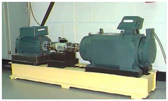
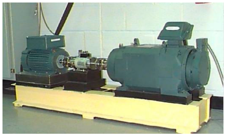
This section evaluates the method on the Case Western Reserve University (CWRU) rolling bearing dataset [31], for which the sampling rates, the loads, the fault sizes and the fault-creation method are all documented by the data provider. The quantitative evaluation reported here is restricted to the discrimination between inner-ring and outer-ring faults; the healthy and ball-fault states are used qualitatively in the following text and are discussed at the end of this section. This dataset was collected on the device shown in Figure 11.

Figure 11. Bearing experiment platform at Case Western Reserve University.

The drive-end and fan-end bearings were selected from the dataset for analysis. The bearing model is the 6205-2RS JEM SKF deep-groove ball bearing for the drive end and the 6203-2RS JEM SKF bearing for the fan end, with sampling frequencies of 12,000 Hz and 48,000 Hz, as shown in Table 7. In the numbering of the data provider, the drive-end records at 12 kHz are 105–108, 169–172, 209–212 and 3001–3004 (inner ring) and 130–133, 197–200 and 234–237 (outer ring), and those at 48 kHz are 109–112, 174–177, 213–215 and 217 (inner ring) and 135–138, 201–204 and 238–241 (outer ring); the fan-end records are 270–273, 274–277 and 278–281 (inner ring) and 294–297, 313 and 315 (outer ring). The outer-ring records are those with the defect centred in the load zone (6 o’clock). The records span the four motor loads of the dataset, 0, 1, 2 and 3 hp, corresponding to approximate shaft speeds of 1797, 1772, 1750 and 1730 rpm; the theoretical characteristic frequency is computed for each record from its own shaft speed.

Table 7. Classification of faulty bearings.

Fault Description	Sampling Rate (Hz)	Fault Type	Number of Signals	Sampling Points
Drive end	12,000	Inner ring	16	1200
		Outer ring	12	1200
	48,000	Inner ring	12	1200
		Outer ring	12	1200
Fan end	12,000	Inner ring	12	1200
		Outer ring	6	1200

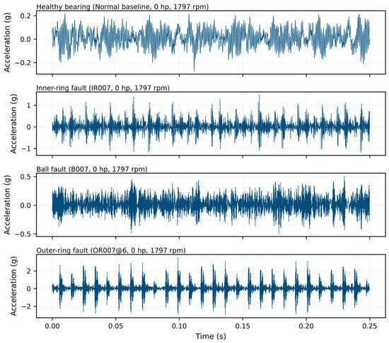
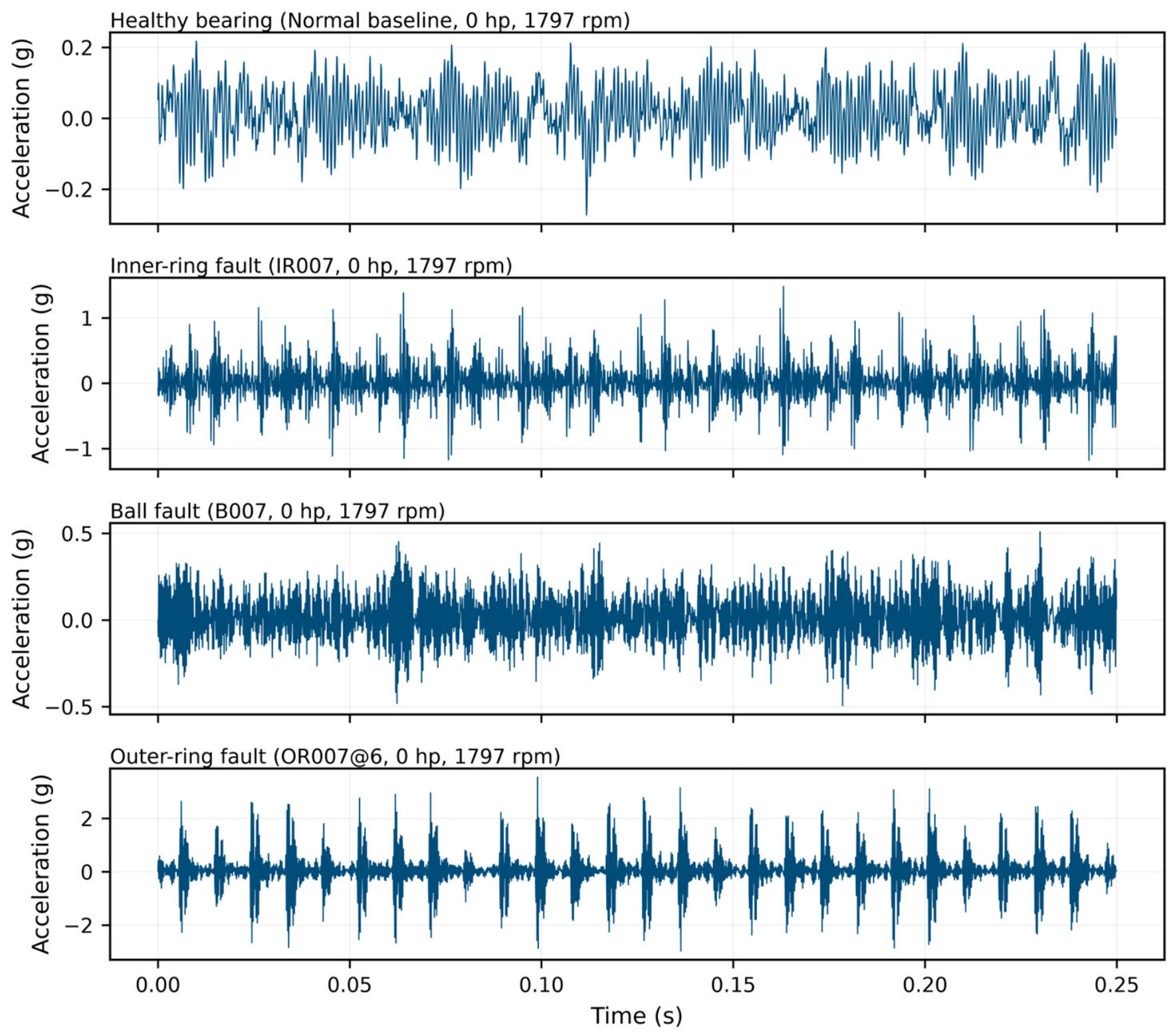
Figure 12 shows the time-domain waveforms of the drive-end signals of the four bearing states analysed: the normal baseline and the inner-ring, ball and outer-ring faults, all recorded at 12 kHz under a 0 hp load at approximately 1797 rpm. The normal signal has a broadband, non-impulsive character with no repeating pattern. The inner-ring and outer-ring signals, in contrast, contain clearly periodic impulse trains. In the case of the outer-ring fault the impulses are almost uniformly spaced, which is consistent with a defect located at a fixed angular position relative to the load zone. The ball-fault signal occupies an intermediate position: its amplitude is markedly lower than that of the outer-ring case and its impulses are less regularly spaced, which is consistent with the ball defect entering and leaving the load zone as the cage rotates.

Figure 12. Time-domain waveforms of the drive-end signals of the four bearing states. From top to bottom: normal baseline, inner-ring fault, ball fault and outer-ring fault.

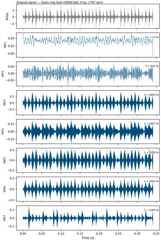
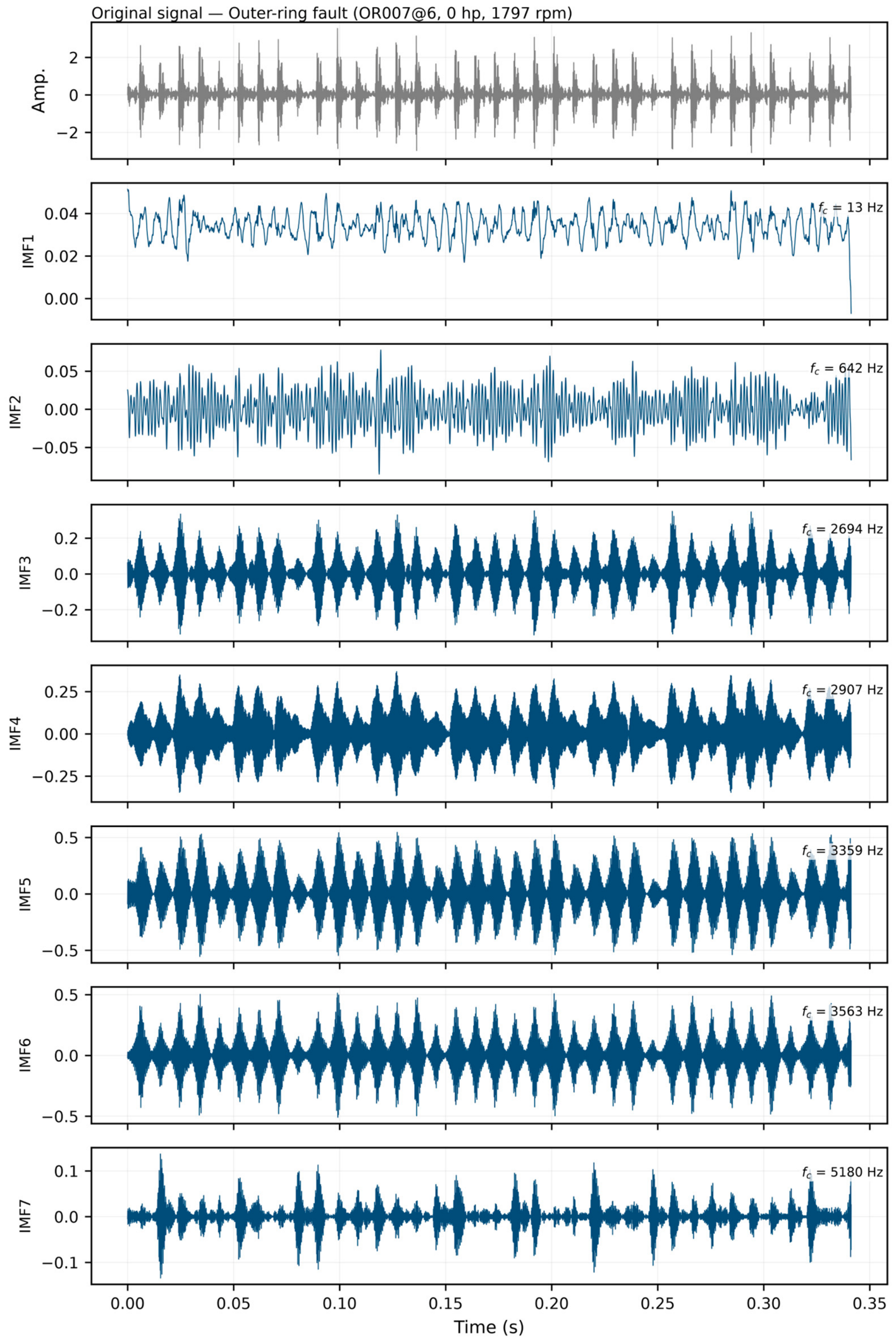
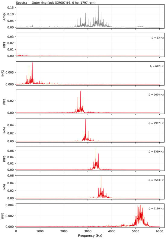
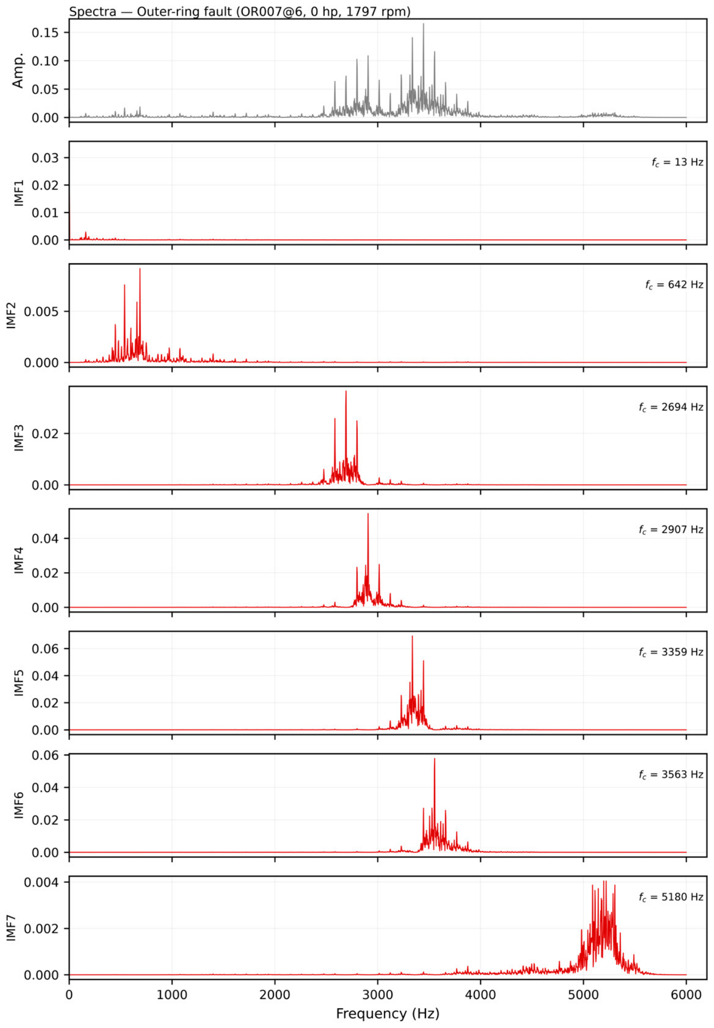
The VMD decomposition of the outer-ring signal, using parameters selected by the GOOSE algorithm, is shown in Figure 13. The signal is separated into seven modes whose centre frequencies progress from the low-frequency end up to the high-frequency resonance band. The first mode captures the slow low-frequency oscillation of the record, with a centre frequency of about 13 Hz, and the remaining modes are distributed between roughly 0.6 kHz and 5.2 kHz, each confined to its own band. The periodic impulses associated with the defect are visible in the modes lying between about 2.7 and 3.6 kHz, that is, across the resonance band excited by the impacts. The corresponding spectra are shown in Figure 14: the frequency content of each mode is confined to a distinct band, and the resonance band carrying the fault information is clearly separated from the low-frequency shaft component and from the higher-frequency noise.

Figure 13. VMD decomposition of the outer-ring fault signal with the parameters selected by GOOSE.

Figure 14. Spectra of the original outer-ring signal and of the modes obtained by VMD.

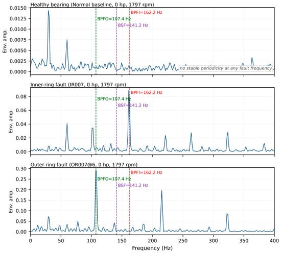
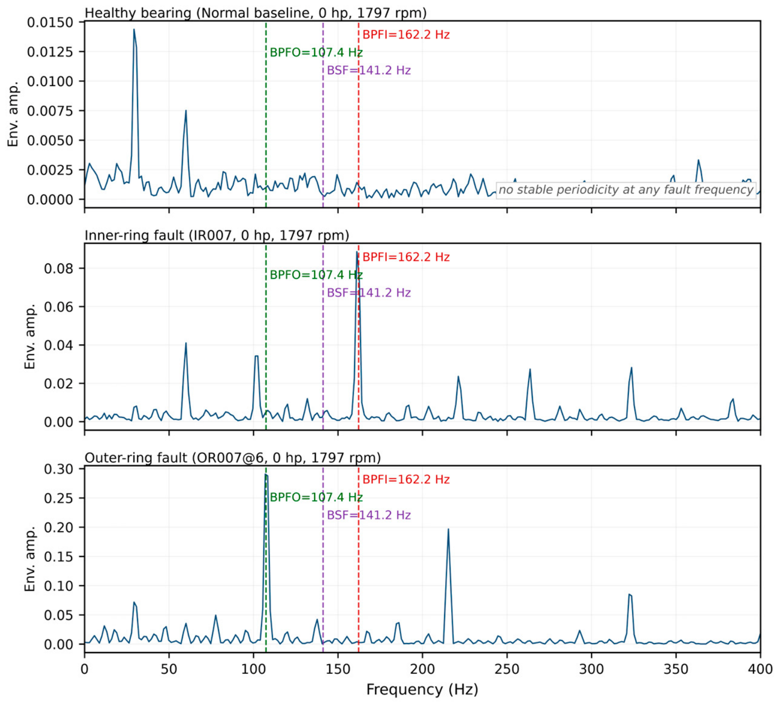
To demonstrate that the identified periodicities originate from the defects rather than from the decomposition itself, Figure 15 compares the envelope spectra of the normal, inner-ring and outer-ring signals. For the inner-ring signal, the dominant peak occurs at 161.1 Hz, which coincides with the theoretical ball-pass frequency of the inner ring, BPFI = 5.4152 × fr = 162.19 Hz at 1797 rpm, and its second and third harmonics are also visible. For the outer-ring signal, the dominant peak occurs at 106.9 Hz, matching the theoretical ball-pass frequency of the outer ring, BPFO = 3.5848 × fr = 107.36 Hz, again with clear harmonics. The amplitude of the dominant peak exceeds the background level of the envelope spectrum by a factor of 49.8 for the inner-ring case and 87.4 for the outer-ring case. For the normal signal, by contrast, no peak appears at any of the characteristic frequencies; the envelope energy remains concentrated at the shaft frequency (29.3 Hz) and its harmonics, and the peak-to-background ratio at the characteristic frequencies does not exceed 1.8. These spectra show that the characteristic frequencies of the two defects are present in the measured signals and can be recovered directly from the raw data, which is a necessary condition for the element-analysis procedure to succeed. They are, however, an independent check that the defect frequencies are physically present rather than a validation of the element-analysis procedure itself; that validation is provided by the agreement between the element-analysis period and the theoretical characteristic frequency, as reported in Table 6.

Figure 15. Envelope spectra of the drive-end signals of the normal, inner-ring and outer-ring bearings. The dashed lines mark the theoretical characteristic frequencies BPFI = 162.2 Hz, BPFO = 107.4 Hz and BSF = 141.2 Hz.

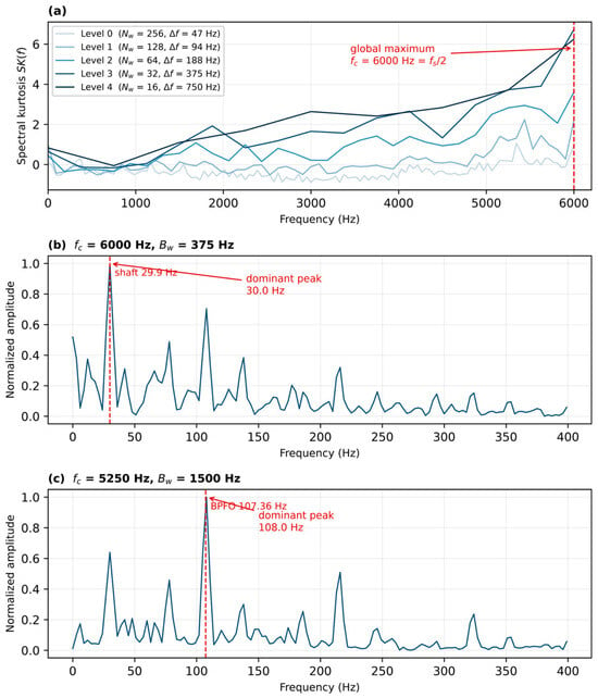
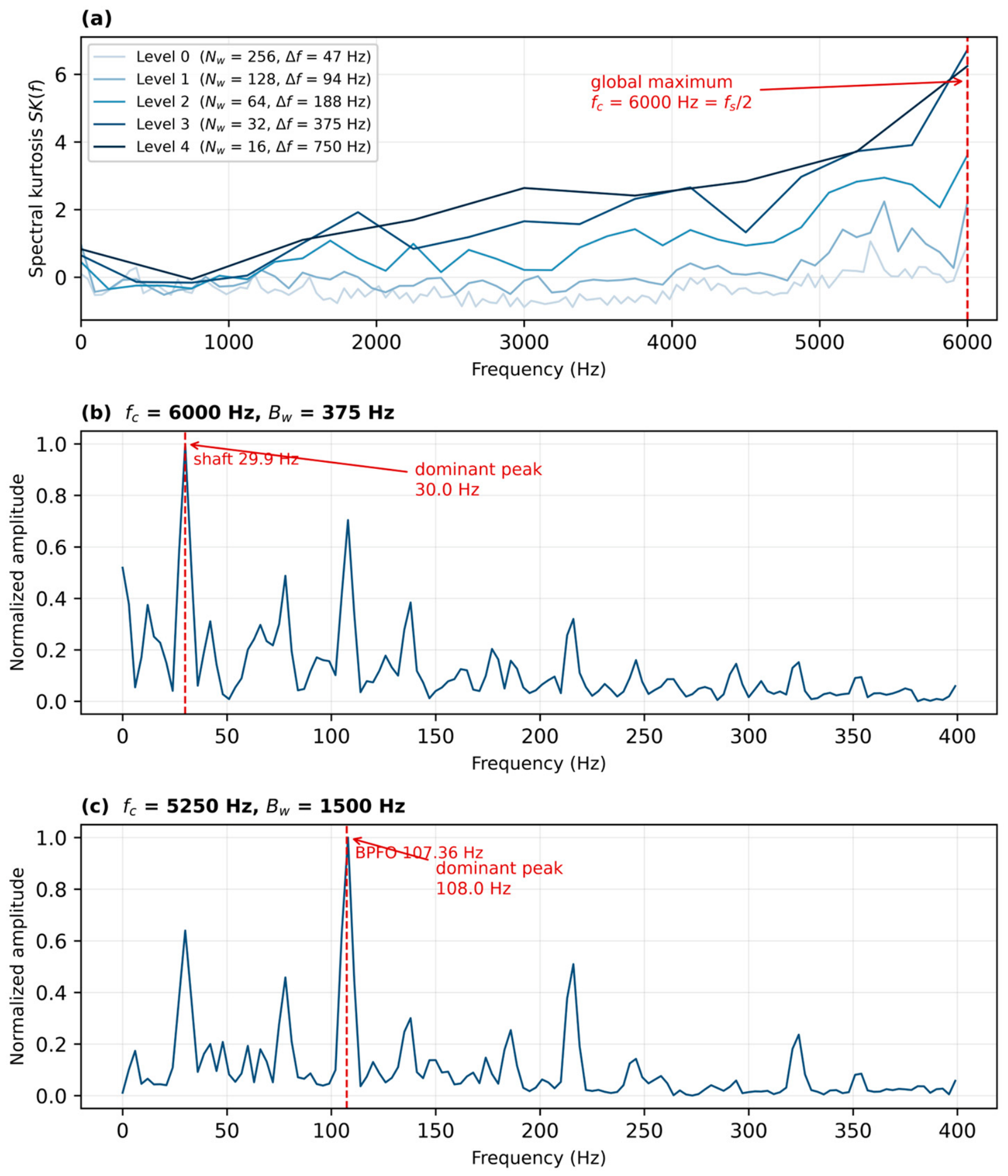
The envelope spectrum is also the most widely used standard technique for bearing fault diagnosis, and it is useful to state explicitly how it relates to the proposed framework and to the standard techniques applied in Figure 15. It is applied here as a reference rather than as a component of the method: it identifies which characteristic frequency is present, but the identification is made by inspecting the spectrum and yields no explicit numerical period, whereas the proposed framework returns the period of the impact events directly and compares it with the theoretical value. As a second reference, the fast kurtogram was applied to the same outer-ring signal. Its spectral kurtosis increases towards the Nyquist frequency and its maximum falls on the boundary at 6000 Hz with a bandwidth of 375 Hz, so the band it selects is not unique; demodulating this band recovers the shaft frequency rather than the ball-pass frequency. A wider band, 4.5–6 kHz, does recover BPFO = 107.4 Hz, as shown in Figure 16c; a band centred on the fault resonance at 2.5–3.5 kHz recovers it with a peak-to-background ratio of 83.7. An automated envelope-peak criterion was then applied to all 70 records, with the envelope spectrum taken over the whole of each record; each record is assigned to the class whose characteristic frequency shows the larger peak-to-background ratio within the same ±3 Hz window: 61 of the 70 records are classified correctly (87.1%), against 69 for the proposed method. The nine failures fall into two groups: the four inner-ring records of the largest fault diameter, which were seeded in NTN bearings so that the characteristic frequencies of the SKF 6205 do not apply to them, and five records in which the strongest peak within the window is not the fault line. If the demodulation band is chosen automatically by the fast kurtogram instead of being taken over the full band, the criterion classifies 55 records correctly (78.6%). The kurtogram therefore still has to be told where to look, whereas the proposed framework obtains the period without any band-selection step.

Figure 16. Fast kurtogram of the outer-ring signal and the envelope spectra obtained from the selected bands: (a) spectral kurtosis at five levels; (b) demodulation of the band with the global maximum (6000 Hz, 375 Hz); (c) demodulation of a wider band centred at 5250 Hz (4.5–6 kHz).

The GOOSE algorithm was used to optimize the VMD parameters of each vibration signal. The signal was decomposed using the optimized parameters. The components used for each record were selected on the same two indicators, the excess kurtosis and the correlation coefficient, as described in Section 3. Element analysis was used to analyse and diagnose the fault type of the best component and its reconstructed signal. Fifteen iterations were allowed for these records. For the two records analysed in detail the optimizer returned K = 8 and α = 834 for the inner-ring case and K = 7 and α = 875 for the outer-ring case, and the element analysis was carried out with γ = 6, β = 53 and μ = 1 for the inner-ring records and γ = 7, β = 74 and μ = 3 for the outer-ring records. The transform maxima are localized to within one sampling interval, so the period estimated from n successive intervals has a relative standard error of the order of $1/n·N_P$, where $N_P$ is the number of samples per period. This corresponds to about 0.3 Hz for the records analysed here. The error range is set to ±3 Hz. The 12 kHz records span 100 ms, which contains 11 to 16 fault periods, while the 48 kHz records span 25 ms, which contains only 3 to 4 periods. Each record is analysed over a segment of 1200 samples—100 ms at 12 kHz and 25 ms at 48 kHz—and the waveforms in Figure 12 and Figure 13 are plotted over longer excerpts so that several impact cycles are visible. The period is estimated as the mean spacing of the transform maxima and each maximum is localized to within one sample, so the sample-based uncertainty of the estimate is small even for the shorter records; the limitation is the small number of intervals available for averaging.

Two aspects of the scope of these results should be made explicit. First, the optimizer is used only to remove the manual selection of K and α; the diagnosis itself is obtained from the period of the reconstructed signal by means of element analysis, and the reported detection rate therefore reflects the accuracy of that physical criterion rather than the performance of the optimizer. Second, no comparison between GOOSE and other metaheuristics under a common fitness function, population size and search range was carried out in this work, and no claim about their relative efficiency is therefore made. Comparative studies of this kind do exist in the literature [14,15,16,17], but each was conducted within its own framework and with its own search settings, so their results are not directly transferable to the present case.

The diagnostic results in Table 8 show that for bearings with inner- and outer-ring faults in the Case Western Reserve University dataset, the method proposed in this paper achieves a fault-recognition rate of 98.57%, indicating high accuracy.

Table 8. Diagnosis results of fault types.

Fault Type	Number of Signals	Number of Correctly Diagnosed Cases	Number of Diagnostic Errors (Records)
Inner ring	40	39	1
Outer ring	30	30	0

One of the 40 inner-ring records was not classified correctly, and the circumstances that permit such a failure mark the limit of the acceptance criterion rather than a difficulty with the period estimate. The window is ±3 Hz, which at 162 Hz admits only a 1.9% uncertainty in the shaft speed, whereas the inner-ring characteristic frequency itself falls from 162.2 Hz at 0 hp to 156.1 Hz at 3 hp; the window is therefore no wider than the variation of the very quantity being compared across the load range of the dataset, and the shaft speeds tabulated by the data provider are approximate values. A single record whose operating speed departs a little further from its nominal value than the rest will accordingly fall outside the window even when its period has been estimated correctly. The margin on the two records analysed in detail, reported in Table 9, is consistent with this reading: the four estimated frequencies lie within 1.4 Hz of the theoretical values, about half the tolerance. One further circumstance should be noted for the four inner-ring records at the largest fault diameter: the defects there were seeded in NTN bearings rather than in the SKF 6205 of Table 4. We therefore regard the ±3 Hz tolerance, and not the period estimate, as the binding constraint of the method at this stage; a tolerance expressed as a fraction of the theoretical frequency would be less sensitive to the operating speed.

Table 9. Element analysis results for the two drive-end records examined in detail, compared with the theoretical characteristic frequencies at 1797 rpm.

Record	Component	Estimated Frequency (Hz)	Theoretical Frequency (Hz)	Difference (Hz)
Inner ring (IR007)	IMF6	162.87	162.19	+0.68
	Reconstructed signal	160.77	162.19	−1.42
Outer ring (OR007@6)	IMF1	107.92	107.36	+0.56
	Reconstructed signal	107.76	107.36	+0.40

Two limitations of this evaluation should be stated explicitly. First, the accuracy figure of 98.57% refers to the discrimination between two fault classes, inner-ring and outer-ring, whose characteristic frequencies at a given shaft speed are separated by about 55 Hz; it is therefore a measure of the ability of the method to identify which of two well-separated elements is defective, and not a measure of its ability to separate a defective bearing from a healthy one or to distinguish a ball defect from a raceway defect. The healthy state is examined in Figure 15, where the envelope spectrum of the normal signal shows no component at any of the characteristic frequencies and its envelope energy remains at the shaft frequency and its harmonics. Applying the proposed method itself to the four normal-baseline records of the dataset returns no impact period for any of them: the excess kurtosis of the modes remains below the acceptance threshold of three, so no component is retained, and none of the records is classified as faulty. No false alarm is therefore produced on the healthy state. The ball-fault signal is included in Figure 12, where its impulses are markedly weaker and less regularly spaced than those of the raceway faults.

5. Conclusions

This paper has proposed a rolling bearing fault diagnosis method that combines GOOSE-optimized VMD with generalized Morse wavelet element analysis. The mode number K and the penalty factor α are determined adaptively by GOOSE and no longer have to be set by hand. Because the fitness values of different entropies are not directly comparable, the four criteria—permutation, sample, information and envelope entropy—were assessed through the decompositions they produced; on this basis, permutation entropy was adopted. This is because it is the criterion most closely related to the periodic impulses produced by a defect and because the decomposition it produces separates the fault-related components most clearly; it was not selected for its computation time. Element analysis then converts the selected modes into a physical quantity: for the self-built test rig the period of the reconstructed signal, 0.00616 s (162.38 Hz), agrees closely with the theoretical inner-ring fault characteristic frequency of 162.46 Hz at 1800 rpm, so that the fault type follows from a comparison between two computed quantities, the impact period returned by the element analysis and the theoretical characteristic frequency, and requires neither the inspection of an envelope spectrum nor the selection of a demodulation band. Meanwhile, 69 of the 70 signals on the CWRU dataset are diagnosed correctly—a recognition rate of 98.57% that covers both inner- and outer-ring faults.

Several limitations should nevertheless be acknowledged. The self-built test rig covers only a single fault type, rotational speed and load, so the generality of the method is demonstrated mainly on the public dataset; compound faults and variable-speed or variable-load conditions were not considered; and the framework is not claimed to outperform data-driven methods in classification accuracy, its advantage being that it requires no labelled training data and remains interpretable at every stage. In addition, the search ranges of K and α, the GOOSE population size and iteration number, and the Morse wavelet parameters were all determined empirically, and no systematic sensitivity analysis of the diagnosis to K and α, or comparison of the optimized parameters with fixed ones, has yet been carried out. Furthermore, no controlled comparison of GOOSE against PSO, GWO or WOA under a common fitness function, population size and search range was carried out, so the present work makes no claim about the relative optimization efficiency of these algorithms.

Future work will therefore extend the method to a larger set of healthy records, to ball and compound faults, and to variable-speed conditions; make the Morse wavelet parameters and the GOOSE search ranges self-adaptive so as to reduce the remaining empirical settings; compare GOOSE systematically with PSO, GWO and WOA in terms of both optimization efficiency and decomposition quality; and explore the framework as a complement to data-driven methods—for instance, by supplying physical labels or priors to deep-learning models when labelled data are scarce.

References

- Hou, J.; Lu, X.; Zhong, Y.; He, W.; Zhao, D.; Zhou, F. A comprehensive review of mechanical fault diagnosis methods based on convolutional neural network. J. Vibroeng. 2024, 26, 44–65. [Google Scholar] [CrossRef] [Scilit]
- Hu, A.; Ma, W.; Tang, G. Fault Feature Extraction Method for Rolling Bearings Based on Ensemble Empirical Mode Decomposition and Kurtosis Criterion. Proc. CSEE 2012, 32, 106–111+153. [Google Scholar] [CrossRef]
- Huang, N.E.; Shen, Z.; Long, S.R.; Wu, M.C.; Shih, H.H.; Zheng, Q.; Yen, N.-C.; Tung, C.C.; Liu, H.H. The empirical mode decomposition and the Hilbert spectrum for nonlinear and non-stationary time series analysis. Proc. R. Soc. Ser. A Math. Phys. Eng. Sci. 1998, 454, 903–995. [Google Scholar] [CrossRef] [Scilit]
- Wu, Z.; Huang, N.E. Ensemble Empirical Mode Decomposition: A Noise-Assisted Data Analysis Method. Adv. Adapt. Data Anal. 2009, 1, 1–41. [Google Scholar] [CrossRef] [Scilit]
- Dragomiretskiy, K.; Zosso, D. Variational Mode Decomposition. IEEE Trans. Signal Process. 2014, 62, 531–544. [Google Scholar] [CrossRef] [Scilit]
- Li, L.; Meng, W.; Liu, X.; Fei, J. Research on Rolling Bearing Fault Diagnosis Based on Variational Modal Decomposition Parameter Optimization and an Improved Support Vector Machine. Electronics 2023, 12, 1290. [Google Scholar] [CrossRef] [Scilit]
- Ye, M.; Yan, X.; Jia, M. Rolling Bearing Fault Diagnosis Based on VMD-MPE and PSO-SVM. Entropy 2021, 23, 762. [Google Scholar] [CrossRef] [Scilit]
- Xu, W.; Hu, J. A Novel Parameter-Adaptive VMD Method Based on Grey Wolf Optimization with Minimum Average Mutual Information for Incipient Fault Detection. Shock Vib. 2021, 2021, 6640387. [Google Scholar] [CrossRef] [Scilit]
- Wang, X.; Liu, X.; Wang, J.; Xiong, X.; Bi, S.; Deng, Z. Improved Variational Mode Decomposition and One-Dimensional CNN Network with Parametric Rectified Linear Unit (PReLU) Approach for Rolling Bearing Fault Diagnosis. Appl. Sci. 2022, 12, 9324. [Google Scholar] [CrossRef] [Scilit]
- Wang, Y.; Zhang, S.; Cao, R.; Xu, D.; Fan, Y. A Rolling Bearing Fault Diagnosis Method Based on the WOA-VMD and the GAT. Entropy 2023, 25, 889. [Google Scholar] [CrossRef] [Scilit]
- Li, J.; Chen, W.; Han, K.; Wang, Q. Fault Diagnosis of Rolling Bearing Based on GA-VMD and Improved WOA-LSSVM. IEEE Access 2020, 8, 166753–166767. [Google Scholar] [CrossRef] [Scilit]
- Wang, H.; Yang, T.; Han, Q.; Luo, Z. Approach to the Quantitative Diagnosis of Rolling Bearings Based on Optimized VMD and Lempel-Ziv Complexity under Varying Conditions. Sensors 2023, 23, 4044. [Google Scholar] [CrossRef] [Scilit]
- Lei, X.; Lu, N.; Chen, C.; Wang, C. An AVMD-DBN-ELM Model for Bearing Fault Diagnosis. Sensors 2022, 22, 9369. [Google Scholar] [CrossRef] [Scilit]
- Yang, J.; Li, X. An Integrated Mechanical Fault Diagnosis Framework Using Improved GOOSE-VMD, RobustICA, and CYCBD. Machines 2025, 13, 631. [Google Scholar] [CrossRef] [Scilit]
- Zhou, J.; Xiao, M.; Niu, Y.; Ji, G. Rolling Bearing Fault Diagnosis Based on WGWOA-VMD-SVM. Sensors 2022, 22, 6281. [Google Scholar] [CrossRef] [Scilit]
- Jin, Z.; Chen, G.; Yang, Z. Rolling Bearing Fault Diagnosis Based on WOA-VMD-MPE and MPSO-LSSVM. Entropy 2022, 24, 927. [Google Scholar] [CrossRef] [Scilit]
- Shui, X.; Rong, Z.; Dan, B.; He, Q.; Yang, X. Tool Wear State Identification Based on the IWOA-VMD Feature Selection Method. Machines 2024, 12, 184. [Google Scholar] [CrossRef] [Scilit]
- Antoni, J. Fast computation of the kurtogram for the detection of transient faults. Mech. Syst. Signal Process. 2007, 21, 108–124. [Google Scholar] [CrossRef] [Scilit]
- Miao, Y.; Zhang, B.; Li, C.; Lin, J.; Zhang, D. Feature Mode Decomposition: New Decomposition Theory for Rotating Machinery Fault Diagnosis. IEEE Trans. Ind. Electron. 2023, 70, 1949–1960. [Google Scholar] [CrossRef] [Scilit]
- Hou, L.; Zhao, J.; Dun, S.; Cai, Y.; Yang, Y.; Xu, J.; Sun, C. Feature Extraction of Weak-Bearing Faults Based on Laplace Wavelet and Orthogonal Matching Pursuit. Shock Vib. 2022, 2022, 8154492. [Google Scholar] [CrossRef] [Scilit]
- Spirto, M.; Malfi, P.; Nicolella, A.; Melluso, F.; Cosenza, C.; Savino, S.; Niola, V. Fault Detection of Electric Motors via Symmetrized Dot Pattern-Based Features. Int. J. Mech. Syst. Dyn. 2026, 6, 445–459. [Google Scholar] [CrossRef] [Scilit]
- Marticorena, M.; García Peyrano, O. Rolling Bearing Condition Monitoring Technique Based on Cage Rotation Analysis and Acoustic Emission. J. Dyn. Monit. Diagn. 2022, 1, 57–65. [Google Scholar] [CrossRef] [Scilit]
- Bandt, C.; Pompe, B. Permutation Entropy: A Natural Complexity Measure for Time Series. Phys. Rev. Lett. 2002, 88, 174102. [Google Scholar] [CrossRef] [Scilit]
- Liu, H.; Li, H.; Wang, R.; Zhu, H.; Zhang, J. Application of Variational Mode Decomposition and Multiscale Permutation Entropy in Rolling Bearing Failure Analysis. Shock Vib. 2022, 2022, 7294795. [Google Scholar] [CrossRef] [Scilit]
- Richman, J.S.; Moorman, J.R. Physiological time-series analysis using approximate entropy and sample entropy. Am. J. Physiol. Heart Circ. Physiol. 2000, 278, H2039–H2049. [Google Scholar] [CrossRef] [Scilit]
- Zhuang, D.; Liu, H.; Zheng, H.; Xu, L.; Gu, Z.; Cheng, G.; Qiu, J. The IBA-ISMO Method for Rolling Bearing Fault Diagnosis Based on VMD-Sample Entropy. Sensors 2023, 23, 991. [Google Scholar] [CrossRef] [Scilit]
- Hamad, R.K.; Rashid, T.A. GOOSE algorithm: A powerful optimization tool for real-world engineering challenges and beyond. Evol. Syst. 2024, 15, 1249–1274. [Google Scholar] [CrossRef] [Scilit]
- Lilly, J.M.; Olhede, S.C. Generalized Morse Wavelets as a Superfamily of Analytic Wavelets. IEEE Trans. Signal Process. 2012, 60, 6036–6041. [Google Scholar] [CrossRef] [Scilit]
- Dai, H.; Wang, Y.; Li, Z. Rolling Bearing Fault Diagnosis Based on Element Analysis. J. Electron. Meas. Instrum. 2022, 36, 157–165. [Google Scholar] [CrossRef]
- Lilly, J.M. Element analysis: A wavelet-based method for analysing time-localized events in noisy time series. Proc. R. Soc. A Math. Phys. Eng. Sci. 2017, 473, 20160776. [Google Scholar] [CrossRef] [Scilit]
- Smith, W.A.; Randall, R.B. Rolling element bearing diagnostics using the Case Western Reserve University data: A benchmark study. Mech. Syst. Signal Process. 2015, 64–65, 100–131. [Google Scholar] [CrossRef] [Scilit]
Disclaimer/Publisher’s Note: The statements, opinions and data contained in all publications are solely those of the individual author(s) and contributor(s) and not of MDPI and/or the editor(s). MDPI and/or the editor(s) disclaim responsibility for any injury to people or property resulting from any ideas, methods, instructions or products referred to in the content. |
© 2026 by the authors. Licensee MDPI, Basel, Switzerland. This article is an open access article distributed under the terms and conditions of the Creative Commons Attribution (CC BY) license.