


Abstract
The classical one-dimensional electroosmotic consolidation theory assumes a linear potential distribution independent of time, thereby neglecting the influence of spatiotemporal evolution of soil electrical properties on the consolidation process. To address this limitation, a one-dimensional electroosmotic model test is conducted in this study, revealing the spatiotemporal evolution characteristics of the electric potential field. The results indicate that changes in electrode-soil interfacial properties and the nonuniform evolution of soil electrical parameters are the primary factors responsible for the redistribution of the potential field. On this basis, the Physics-Informed Neural Networks (PINNs) method is introduced for potential field reconstruction, fully leveraging the combination of physical constraints and data-driven approaches to achieve spatial densification of the potential field under sparse observations. Furthermore, a surrogate model characterizing the spatiotemporal evolution of the potential field is constructed and embedded into the governing equation of electroosmotic consolidation as a nonhomogeneous source term, which is then solved numerically using the finite difference method. The computational results demonstrate that the negative excess pore water pressures obtained by the proposed method exhibit smaller magnitudes than those predicted by the classical theory, with the discrepancies primarily concentrated near the anode, reaching a maximum of approximately 120 kPa. The proposed approach provides a feasible pathway for electroosmotic consolidation analysis that accounts for the spatiotemporal evolution of the electric potential field.
1. Introduction
Soft clay is characterized by high water content, high compressibility, and low permeability. When conventional preloading methods are applied to such soils, the consolidation process often requires a prolonged duration and exhibits low drainage efficiency. Electro-osmotic consolidation, by contrast, applies a voltage across the soil mass and utilizes the resulting electrical potential gradient to drive directional flow of pore water [1,2]. Since the electro-osmotic flow is governed by the potential gradient, this method proves particularly effective for fine-grained soils with hydraulic conductivity below m/s [3]. Following its successful engineering application and validation [1,4], the method has attracted considerable research attention. However, the low efficiency and high energy consumption in the later stages of electro-osmotic treatment have restricted its further engineering adoption. Consequently, studies on influencing factors and theoretical models related to this issue have become prominent research topics in the current investigation of electro-osmotic consolidation and drainage.
The theoretical foundation of electro-osmotic consolidation was established by Esrig [5], and subsequently extended to combined surcharge loading and electrode polarity reversal by Wan [2]. Since then, extensive research has been conducted on both analytical and numerical solutions. In terms of numerical methods, these have been introduced to address electro-osmotic consolidation under complex conditions [6,7,8,9]. On the analytical front, researchers have progressively incorporated nonlinear variations in soil parameters [10,11], large-strain theory [7,8,12,13], and ion-transport-dependent electro-osmotic permeability models [14]. Effective voltage decay is a critical issue affecting the later-stage efficiency of electro-osmosis; existing studies have addressed this through modified consolidation theories [15] and piecewise inheritance strategies [16]. Meanwhile, experimental evidence has revealed the existence of nonlinear potential distributions, prompting scholars to develop consolidation models that account for such nonlinear voltage profiles [17,18,19]. The electro-osmotic consolidation behavior in layered soils has also attracted attention, with analytical solutions for double-layer [20], multi-layer [21,22], and permeable anode [23] configurations revealing the significant influence of soil stratification and boundary permeability on consolidation behavior. Closed-form solutions for axisymmetric electro-osmotic consolidation incorporating smear effects have also been derived [24,25]. In the later stages of electro-osmosis, the soil transitions from a saturated to an unsaturated state; in response to this actual change, a series of unsaturated models have been proposed, incorporating factors such as deformation-voltage coupling, non-uniform initial water content distribution, semi-permeable boundary conditions, and free-strain assumptions [26,27,28,29,30,31,32]. To mitigate the inherent limitations of single-method approaches, combined multi-method techniques have gained attention and development, with corresponding analytical solutions derived under various loading schemes and electrode configurations [11,33,34,35]. Multi-field coupled models incorporating chemical field effects and ion transport have further enriched the theory of electro-osmotic consolidation [36], and the technique has also demonstrated application potential in special scenarios such as synergistic dehydration and remediation of copper-contaminated sludge [37] and electro-osmotic pre-thawing of frozen saline soil [38].
Moreover, energy consumption has received increasing attention, with related studies proposing evaluation methods for energy conversion efficiency [39], pulsed direct current techniques [40], and optimization schemes for electrode materials and arrangements [34,41,42]. However, most existing theoretical models rely on simplifying assumptions such as constant or linear voltage distributions and homogeneous soil conditions, while conventional numerical methods struggle to achieve integration between experimentally measured data and theoretical models. In recent years, Physics-Informed Neural Networks (PINNs) have provided a new paradigm for solving partial differential equations. Raissi et al. [43] first proposed the PINN framework, enabling dual-driven solutions that combine data and physical laws by embedding physical equations into the loss function [44,45]. To date, PINNs have achieved preliminary applications in fields such as solid mechanics [46], elastoplastic constitutive modeling of soils [47], and pile-soil dynamic interaction [48], but have not yet been reported in the field of electro- osmotic consolidation.
Although existing studies have achieved fruitful progress in incorporating nonlinearity and large-strain effects into theoretical models of electro-osmotic consolidation [7,8,10,11,12,13,34], the electro-osmotic drainage method still suffers from low later-stage efficiency and high energy consumption in engineering practice. Current theoretical models fail to adequately account for the influence of voltage loss and variations in potential distribution on pore water pressure during the electro-osmotic process. The electric potential field is typically assumed on the basis of electrostatic field theory (i.e., satisfying the Laplace equation). This idealized assumption neglects the non-ideal characteristics of the actual potential distribution in soils, leading to calculated results that tend to overestimate the consolidation effectiveness [2,5,15,16,17]. To address the above limitations, this paper proposes a one-dimensional electro-osmotic consolidation computational framework that integrates a physics-informed neural network with the finite difference method. First, the PINN approach is employed to reconstruct the electric potential distribution at each monitoring time instant, combining physical constraints with measured data to achieve spatial refinement of the potential field under sparse observations, and a spatiotemporally continuous function of the potential field is constructed via neural network fitting. Subsequently, the one-dimensional electro-osmotic consolidation equation is directly discretized, and the aforementioned potential surrogate model is embedded into the finite difference scheme as a non-homogeneous source term, enabling the solution of pore water pressure under the actual potential distribution. Concurrently, a one-dimensional electro-osmotic model test is conducted to analyze the intrinsic mechanisms and spatiotemporal distribution characteristics of the potential field evolution. The proposed computational strategy is validated using the experimental data, and the results demonstrate its satisfactory effectiveness and feasibility. This study may provide a quantitative computational tool for mitigating the issues of low efficiency and high energy consumption in the later stages of electro-osmotic drainage.
2. One-Dimensional Electro-Osmotic Test
2.1. Materials and Methods
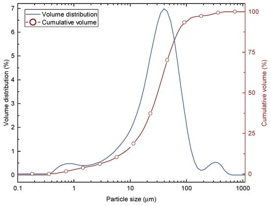
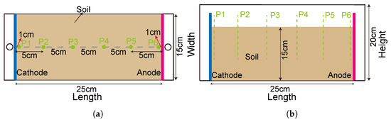
The test soil was taken from a deep excavation project, and its particle size distribution curve is shown in Figure 1. The average water content of the soil at the initial stage of electro-osmosis was 34.6%. The model box (Miller box) has dimensions of 25 cm in length, 15 cm in width, and 20 cm in height, with an additional 2 cm extension on both the left and right sides serving as water collection channels. To monitor the electric potential distribution within the soil during the test, metal probes were pre-embedded at predetermined measuring points. The probes were fabricated from iron wire with a diameter of 2.5 mm and a length of 10 cm, wrapped externally with insulating tape, leaving 1 cm of bare length at the bottom. The embedding depth was uniformly set at 9 cm to ensure that all measuring points were located at the same horizontal level. Stainless steel plate electrodes were employed, with drainage holes opened on the cathode plate to facilitate water discharge, while the anode plate remained unperforated to achieve undrained conditions. The dimensions of the electrode plates matched the cross-section of the model box and could be fixed by embedding them into preset slots. A direct current (DC) power supply was used for the electro-osmotic tests, with a maximum output voltage of 60 V and a maximum output current of 5 A. For convenient potential measurement, the top of each probe was connected to external leads via wires. The potential values were measured using a multimeter, and the circuit current was read directly from the DC power supply panel. A drainage hole was provided at the bottom of the water collection zone on the cathode side, and the discharged water was collected and measured using a beaker.
Figure 1.
Particle size distribution curve of the test soil.
A constant voltage of 25 V was applied throughout the entire period. The test soil was oven-dried, crushed, and re-saturated before being placed into the model box and allowed to stand for 24 h to ensure a uniform distribution of water content within the soil mass. The actual filling height of the soil was 15 cm. The metal probes were numbered P1 to P6 sequentially from the cathode to the anode, with probes P1 and P6 positioned 1 cm away from the cathode and anode plates, respectively, to facilitate estimation of the voltage loss at the soil-electrode interfaces. The layout of the potential measuring points is shown in Figure 2. Specifically, Figure 2a depicts the plan arrangement of the test model box, while Figure 2b displays its elevation. During the test, when the change in the measured mass of discharged water between two consecutive readings was less than 0.5 g, drainage was considered to be essentially complete, and the test could be terminated. According to this criterion, the actual duration of electrification in this test was 102.5 h.
Figure 2.
Experimental model layout diagram. (a) Plan Layout of Experimental Model Box. (b) Elevation of Experimental Model Box.
2.2. Analysis and Discussion of Experimental Results
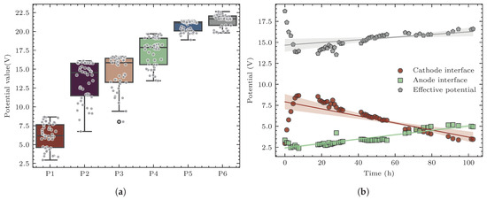
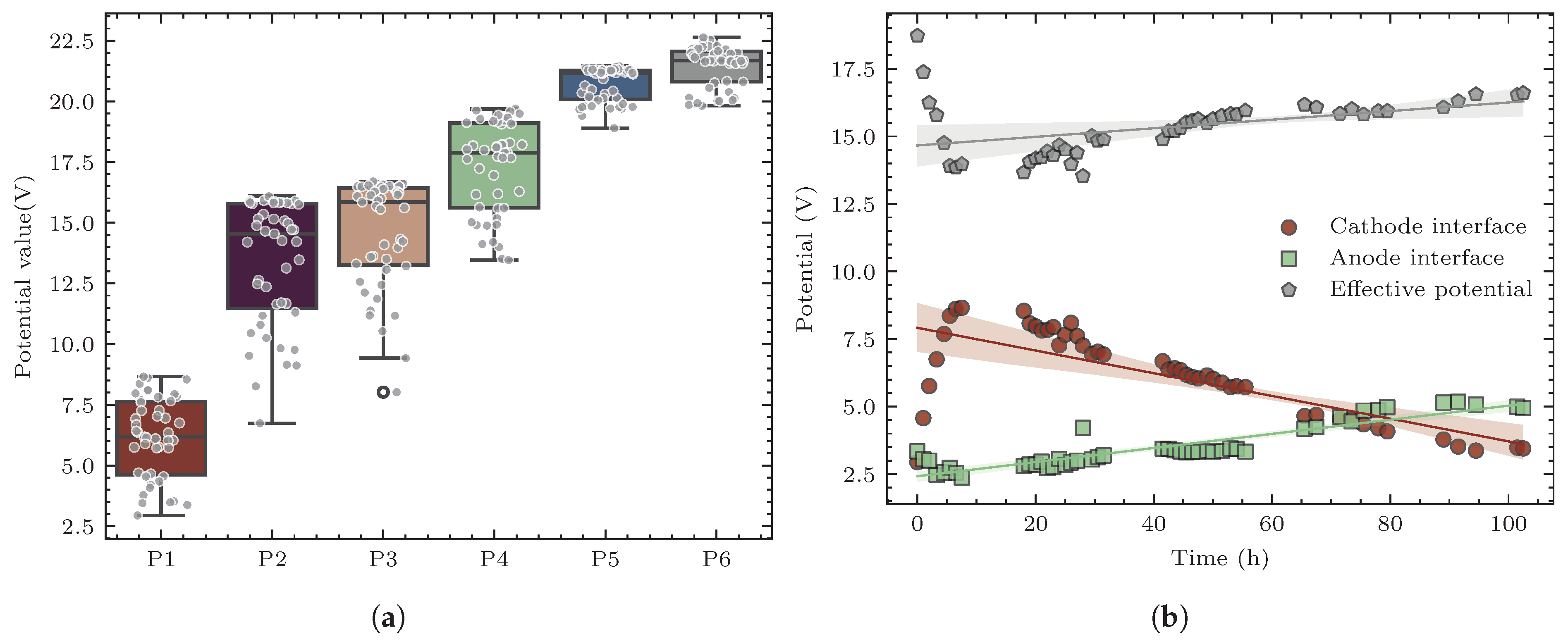
A constant voltage of 25 V was applied throughout the test. After 102.5 h of electrification, the average water content of the soil decreased to 14.7%, and the cumulative drainage mass amounted to 1173.9 g. The initial current was 0.412 A, which dropped to 0.031 A at the end of electro-osmosis, representing a reduction of 92.48%. Metal probes were used to measure the electric potential distribution at different positions within the soil. Probes 1 and 6, located near the cathode and anode, respectively, were employed to estimate the voltage loss at the corresponding electrode-soil interfaces. The potential distributions at all measuring points are shown in Figure 3a, where probes P2 and P3 exhibited the largest potential variations, and overall, the potential variation decreased with proximity to the anode. Since the total applied voltage remained constant at 25 V throughout the test, the total voltage loss consisted of the voltage losses at both the cathode and anode interfaces. Specifically, the difference between the potential measured by probe 6 and the applied total voltage (25 V) characterized the voltage loss at the anode interface; while the cathode potential was approximately taken as the reference zero potential, so the potential value measured by probe 1 directly reflected the voltage loss at the cathode interface. On this basis, the time histories of the interfacial contact voltage losses and the effective soil voltage are presented in Figure 3b. At the initial moment, the cathode interfacial voltage loss was 2.94 V, which increased to 8.54 V after 7.5 h of electro-osmotic drainage and then exhibited a declining trend, reaching 3.45 V at the end of the test. The anode interfacial voltage loss increased from 3.34 V at the initial moment to 4.95 V at the end, exhibiting an approximately linear trend overall. Correspondingly, the effective voltage first decreased significantly and then increased gently, but exhibited an overall decreasing trend. The experimental results indicate that the electrical properties of the electrode-soil interfaces continuously evolved during the electro-osmotic process, leading to a gradual increase in interfacial voltage losses. Consequently, the effective voltage actually acting on the soil and driving pore water drainage remained consistently lower than the applied total voltage, with a particularly notable decrease in the later stage of electro-osmosis. It should be noted that in this experiment, the P1 and P6 probes are located approximately 1 cm from the electrode plate. At this distance, the measured voltage loss includes a portion of the voltage within the soil. Therefore, the interfacial voltage loss results may be overestimated, leading to an overestimation of the total voltage loss.
Figure 3.
Monitoring of electrical potential and effective voltage during electro-osmosis. (a) Box plot of electric potential data at measuring points. (b) Variation curves of effective electro-osmotic voltage and interfacial voltage loss.
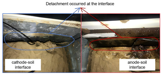
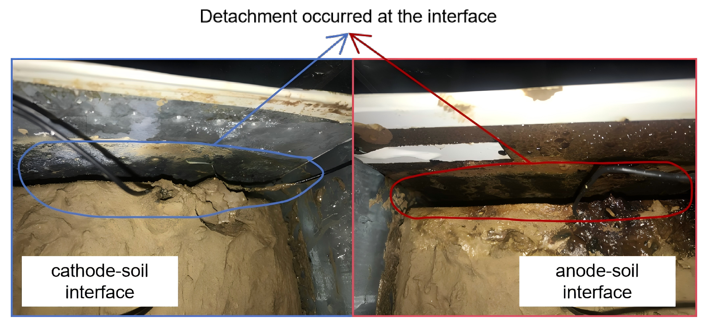
The continuous increase in the aforementioned interfacial voltage loss during the electro-osmotic process can be mainly attributed to the following two factors. First, the corrosion of metal electrodes under electrified conditions weakens the contact between the electrodes and the soil, thereby increasing the interfacial contact resistance, which manifests as an elevation in voltage loss. Second, electro-osmotic drainage induces volumetric shrinkage of the soil; particularly in the later stage of electro-osmosis, a certain degree of separation may occur between the electrodes and the soil, which similarly reduces the contact quality and further exacerbates the interfacial voltage loss. Photographs of the model after the test are shown in Figure 4. Given that both metal electrode corrosion and soil desiccation shrinkage are unavoidable during electro-osmosis, the interfacial voltage loss and the corresponding effective voltage are not constant. This phenomenon has also drawn the attention of other researchers [15,16,17,18]. From the perspective of the physical field, the effective voltage essentially serves as the boundary condition of the electric potential field at the electrode boundaries. Moreover, as this boundary condition evolves with the progress of electro-osmosis, it inevitably induces a reconstruction of the potential field distribution within the spatial domain for the corresponding boundary value problem.
Figure 4.
Photographs of electrode-soil interfaces after testing.
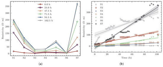
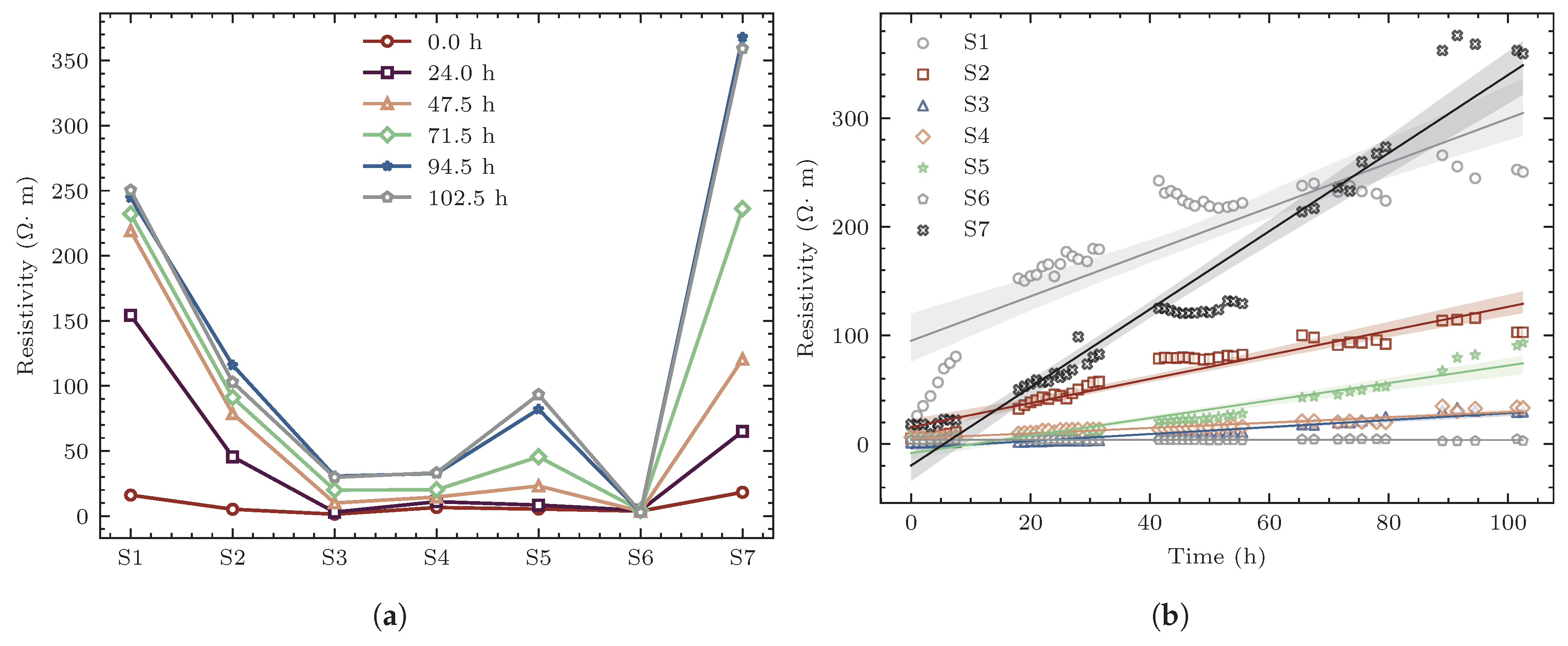
The one-dimensional electro-osmotic model can be approximately treated as a series circuit. According to Ohm’s law, the difference in potential variation amplitude at different positions reflects the variation in soil resistance within the corresponding sections. To further quantitatively analyze the spatiotemporal evolution of electrical resistivity, the soil between the cathode and anode was divided into seven sections bounded by adjacent metal probes, denoted sequentially as S1 to S7. The voltage shared by each section can be converted into the electrical resistivity of the soil in that section. Figure 3 presents the variation characteristics of resistivity in each section. Specifically, Figure 5a shows the spatial distribution of resistivity at different time instants. At the initial moment, the water content distribution in the soil was relatively uniform, and since resistivity is closely related to water content, the initial resistivity also exhibited a relatively uniform distribution. As electro-osmotic drainage proceeded (with the drainage direction from the anode toward the cathode), the extent of water content reduction varied at different positions, leading to non-uniform changes in resistivity. In particular, the resistivity variation at the electrode contact surfaces was significantly greater than that in the central soil mass. Specifically, at the anode contact surface, owing to the undrained condition and the continuous migration of pore water toward the cathode without replenishment, the water content reduction was the largest, and the resistivity increased from an initial value of 18.24 to a final value of 359.27 ; at the cathode contact surface, the resistivity increased from an initial value of 16.06 to 250.40 . Figure 5b shows the time-dependent variation curves of resistivity for each section. It can be observed that the rate and magnitude of resistivity change were most significant at the electrode contact surfaces, and from the cathode toward the anode, the rate of resistivity change exhibited a gradually decreasing trend. The above results indicate that the electrical properties of the soil during electro-osmosis are not constant but exhibit pronounced evolutionary characteristics over time. Meanwhile, due to the directional migration of pore water and the non-uniformity of the soil pore structure, the magnitudes of changes in electrical properties also differed at different spatial locations, resulting in significant spatial non-uniformity of resistivity distribution.
Figure 5.
Monitoring results of soil resistivity during electro-osmotic treatment. (a) Soil resistivity distribution curves at different time instants. (b) Resistivity variation curves for each soil section.
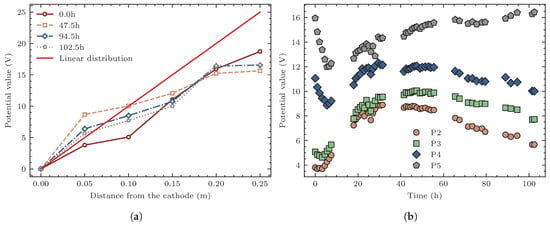
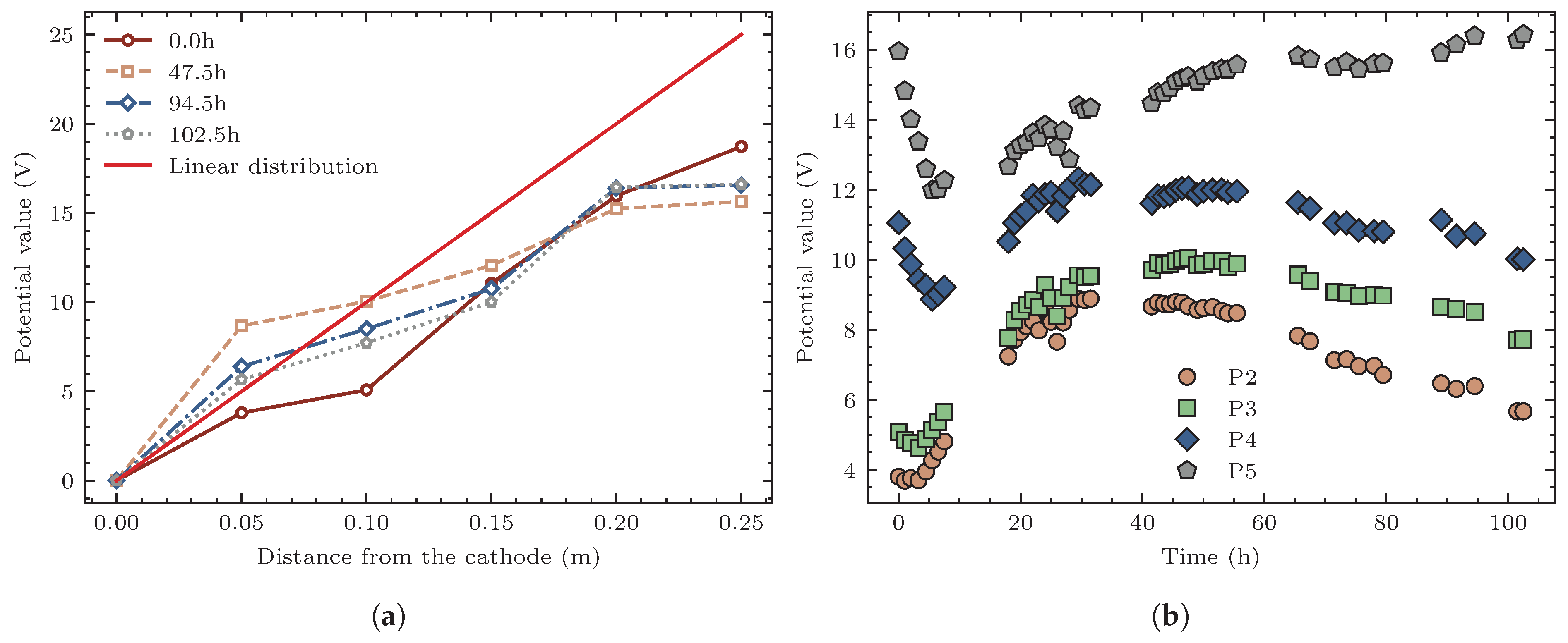
The continuous variation of soil resistivity during electro-osmosis induces a redistribution of the electric field within the soil. Under ideal homogeneous medium conditions, electrostatic field theory predicts a linear potential distribution. However, the heterogeneity of actual soils and the spatiotemporal evolution of resistivity often cause the potential field to deviate from this ideal state [15,16,17,18]. Figure 6 presents the distribution characteristics of the electric potential at each measuring point and their temporal evolution, based on which the above-mentioned deviation can be quantitatively analyzed. Figure 6a shows the effective potential distribution curves at four characteristic time instants (0 h, 47.5 h, 94.5 h, and 102.5 h). It can be observed that the potential distribution within the soil did not strictly follow a linear relationship. In the early to middle stages of electro-osmosis, the potentials at probes P2 and P3, located near the cathode side, exhibited a pronounced increasing trend. In the later stage, however, the potentials at these two measuring points decreased somewhat. Figure 6b further presents the evolution curves of the potential at each measuring point with respect to electrification time. For probes P4 and P5, located near the anode, their potentials decreased significantly at the initial stage of the test, recovered slightly in the middle stage, but exhibited an overall decreasing trend. In contrast, the potentials at probes P2 and P3 on the cathode side continuously increased in the early to middle stages and decreased slightly in the later stage, exhibiting an overall increasing trend. The above variation characteristics indicate that during electro-osmosis, the electrode-soil interfacial effects and the changes in soil matrix resistivity jointly influence the dynamic adjustment of the internal electric field. The potential distribution of the soil during electro-osmotic drainage exhibits dual evolutionary characteristics in both spatial and temporal dimensions. This variation characteristic of the electric potential during electro-osmosis has also been reported by other researchers [15,17,18].
Figure 6.
Distribution and temporal variation of effective electrical potential in soil during electro-osmosis. (a) Effective potential distribution curves at different time instants. (b) Variation curves of effective potential at measuring points.
The experimental results indicate that electrode corrosion and soil shrinkage induced by drainage during electro-osmosis are unavoidable. Both factors directly alter the electrical properties at the electrode-soil contact surfaces, leading to an increase in contact voltage loss and consequently a reduction in electro-osmotic drainage efficiency. The variation in the aforementioned voltage loss essentially reflects a change in the boundary condition of the electric potential field. From the perspective of the potential field, the effective voltage serves as the boundary condition of the potential field, which varies with the electro-osmotic process and constitutes an external factor affecting the potential field distribution. On the other hand, electro-osmotic drainage reduces soil water content, which in turn leads to changes in soil resistivity. Since the extent of water content reduction varies at different locations, the magnitude of resistivity change also exhibits spatial differences, which likewise alters the potential field distribution. This factor originates from the evolution of the soil’s own electrical properties and constitutes an internal factor affecting the potential field. It can thus be concluded that during electro-osmosis, the potential field distribution is jointly governed by external factors (variations in boundary conditions) and internal factors (spatiotemporal evolution of soil resistivity), exhibiting dual spatiotemporal evolutionary characteristics, i.e., temporal evolution and spatial non-uniformity coexist.
3. Computational Method Incorporating Potential Field Evolution
If an excessive number of metal probes or sensors are embedded during the experiment, stress concentration may be induced in the soil, exacerbating the development of soil cracks, thereby interfering with or even interrupting the generation and maintenance of negative pore water pressure during electro-osmosis. Consequently, the electric potential data obtained from actual monitoring is far less than the amount of information required for characterizing the electric potential field. The measured data exhibits significant sparsity, and it is difficult to accurately reconstruct the electric potential field relying solely on data-driven methods. Based on the above analysis, the objective of this study is to achieve an effective description of the spatiotemporal evolution characteristics of the electric potential field under sparse observation conditions, and to embed this description into the transient calculation framework of pore water pressure, so as to more reasonably reflect the actual behavior of electro-osmotic consolidation.
3.1. Strategies for Capturing the Spatiotemporal Evolution Behavior of the Electric Potential Field
Considering the spatiotemporal evolution characteristics of the electric potential field, the potential field function is a function of the spatial coordinate x and time t. Under ideal conditions, the potential field at each time instant satisfies the Laplace equation, as shown in Equation (1).
where is the electric potential field function, which is a function of the spatial coordinate x.
In electro-osmotic tests, the number of metal probe measurement points is limited, and the measured data are markedly sparse. For the reconstruction of the electric potential field at each time instant, a physics-informed neural network (PINN) can be employed to combine physics-driven and data-driven approaches: on one hand, the measured data are used to guide the field distribution; on the other hand, the partial differential equation (PDE) residuals are incorporated as physical constraints to enhance the reliability of the results. Meanwhile, since this problem is a typical boundary value problem, a hard constraint strategy is adopted in the network architecture of the PINN to ensure that the boundary conditions are strictly satisfied, such that the network output exactly matches the boundary conditions of the potential field at the boundaries. In this case, the loss function for network training includes only the PDE residual loss and the measured data residual loss. To balance the influence of the difference between the number of collocation points within the domain and the number of measured data points, a weight is assigned to the loss corresponding to the relatively scarce known data. More comprehensive studies on the PINNs method and its loss formulation can be found in these references [43,44,45,49,50,51]. The specific form of the loss function is given in Equation (2).
where denotes the total loss function with respect to the neural network parameters ; is the residual loss of the governing partial differential equation evaluated at collocation points; is the data loss evaluated at sampled points; and the ratio serves as a weighting factor to balance the two loss terms.
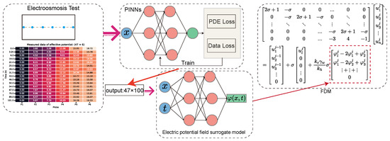
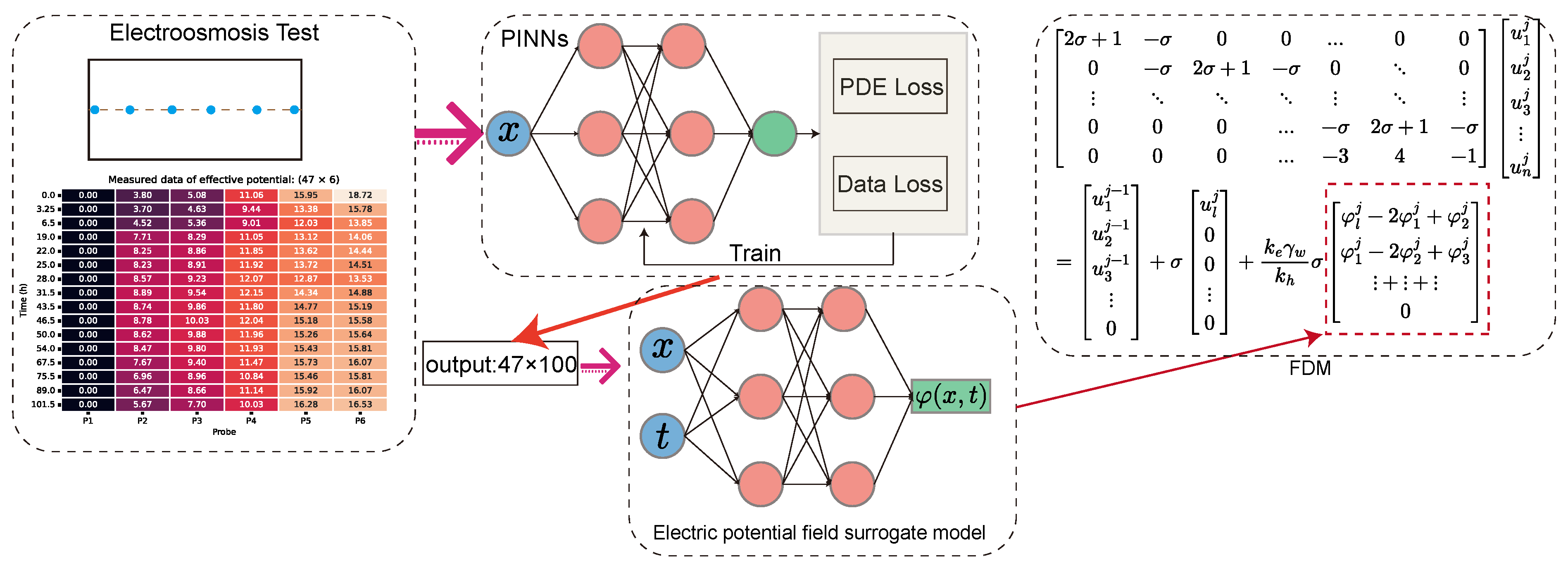
This strategy constructs a surrogate model independently for each monitoring time instant, which can significantly increase the number of effective sampling points of the potential field in the spatial domain, thereby alleviating the issue of feature information loss caused by data sparsity. After completing the PINN computations at each time instant, the spatial distribution of the electric potential at each monitoring time is obtained with enhanced sampling density. To ultimately construct a spatiotemporally continuous potential function , a neural network is employed to fit the discrete dataset that has been spatially upsampled as described above. The trained network can then be regarded as a callable continuous function, serving as the surrogate model for the potential function . By embedding this function into the governing equation of electro-osmotic consolidation for numerical solution, a quantitative assessment of the influence of the spatiotemporal evolution characteristics of the electric potential field on the transient response of pore water pressure can be achieved.
3.2. Finite Difference Formulation of the Governing Equation
In classical one-dimensional electro-osmotic consolidation theory, the electric potential term is simplified as a function that depends only on the spatial coordinate and is independent of time. Based on this assumption, the governing equation can be transformed into a standard parabolic partial differential equation by introducing an intermediate variable, thereby yielding an analytical solution. However, when the spatiotemporal evolution characteristics of the potential field are taken into account, the electric potential term explicitly contains time t, and the intermediate variable transformation is no longer applicable, thus rendering the classical analytical solution path infeasible. Since a surrogate model for has been constructed using PINNs as described above, this potential term can be treated as a known function in the governing equation. To facilitate numerical solution, the term containing is moved to the right-hand side of the equation and treated as a non-homogeneous source term, and the resulting non-homogeneous equation is discretized and solved using the finite difference method (FDM). Furthermore, to preserve flux conservation in the numerical discretization process, the governing equation is rewritten in conservative form. The conservative form of the one-dimensional electro-osmotic consolidation governing equation is given in Equation (3).
where is the excess pore water pressure in the soil during electro-osmosis; is the hydraulic permeability coefficient of the soil; is the electro-osmotic permeability coefficient of the soil; and is the coefficient of volume compressibility of the soil.
After treating the electric potential term as a non-homogeneous source term, the idea of the finite volume method is introduced to preserve flux conservation in the numerical discretization process, ensuring that the fluxes in each local control volume satisfy the conservation property. Specifically, for control volume i, the coordinates of its left and right boundaries are denoted as and , respectively, and the coordinate of its center point is . By integrating the conservative-form governing equation over the spatial interval for this control volume, the integral form of the equation can be obtained, as shown in Equation (4).
After performing the integration, Equation (5) is obtained.
By utilizing the function values at the centers of the adjacent control volumes on the left and right sides, the first-order derivative at the interface is computed using the two-point central difference scheme, yielding Equation (6).
To ensure the stability and convergence of the iterative computation, the backward difference scheme is adopted for the temporal discretization, as shown in Equation (7).
Let
The finite difference form of the governing equation is then given by Equation (9).
The spatial domain is uniformly divided into n elements, yielding nodes, with node numbering starting from 0. The left boundary (cathode) is designated as node 0, and the right boundary (anode) as node n, where l denotes the total length of the soil. In the aforementioned experimental model, the cathode plate is perforated for drainage, resulting in a drainage boundary condition; conversely, the anode plate remains unperforated, constituting an impermeable boundary corresponding to a homogeneous Neumann condition. The boundary conditions are prescribed as follows: at the cathode (), a drained boundary is imposed, satisfying ; at the anode (), an undrained boundary is imposed, satisfying the homogeneous Neumann condition, i.e., . The Neumann condition at the right boundary is described using an independent first-order derivative extrapolation formula, and the last row of the coefficient matrix is modified accordingly. With the above boundary conditions incorporated, the difference equations can be arranged into matrix form, as shown in Equation (10).
To implement the above computational procedure, a dedicated Python 3.14.6 module named pyec was developed, which is capable of fully realizing the proposed computational strategy. Within the pyec module, a one-dimensional MLP-based hard-constraint network is constructed on the PyTorch 2.14.1 framework for PINN computations, and the program automatically iterates through the experimental measurement data to perform PINN computations at each time instant. In addition, an MLP network with dual inputs (spatial coordinate x and time t) is constructed to fit the potential function . Upon completion of training, the surrogate model of the potential field is encapsulated as a callable function, which is directly incorporated into the finite difference computation of the governing equation. The computational strategy and implementation workflow of the above proposed method are illustrated in Figure 7.
Figure 7.
Schematic diagram of the computational strategy.
4. Numerical Validation and Discussion
To validate the effectiveness of the aforementioned computational method, a numerical example is carried out. The computational model is consistent with the aforementioned one-dimensional model test, with the spatial domain being m, the left boundary being drained, the right boundary being undrained, and the initial excess pore water pressure being kPa. The boundary conditions of the electric potential field are adopted from the experimental measurement data, and the total computation duration is consistent with the test, i.e., 102.5 h. First, the PINN method is employed to compute the potential distribution at each monitoring time instant, so as to enhance the spatial sampling density at each time instant. A total of 47 time instants were recorded in the test, with 6 measuring points of potential data per time instant (); after PINN-based densification, the number of sampling points per time instant increased to 100 (). Subsequently, based on the densified potential dataset, an MLP network is adopted for fitting, thereby constructing a spatiotemporally continuous potential function . In the numerical solution, the spatial domain is uniformly divided into 100 elements with 101 nodes; the number of time steps is set to 5001. The soil parameters used for computation are listed in Table 1 [2,3,11,15]. All the above computations are accomplished using the pyec module.
Table 1.
Basic parameters for electro-osmotic consolidation analysis.
4.1. Surrogate Model of the Electric Potential Field
In the PINN computations, the MLP network architecture is 1-40-40-40-1, with the tanh function employed as the activation function. A penalty function concerning the potential boundary coordinates is added to the output layer to ensure that the network output strictly satisfies the boundary conditions at the boundaries. The loss function is the MSELoss, with the number of collocation points for the governing equation being and the number of known potential data points at each monitoring time instant being . The number of training epochs is set to 500. After the PINN computations are completed for each of the 47 monitoring time instants, the neural network is used to increase the number of spatial distribution points from 6 to 100.
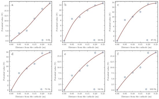
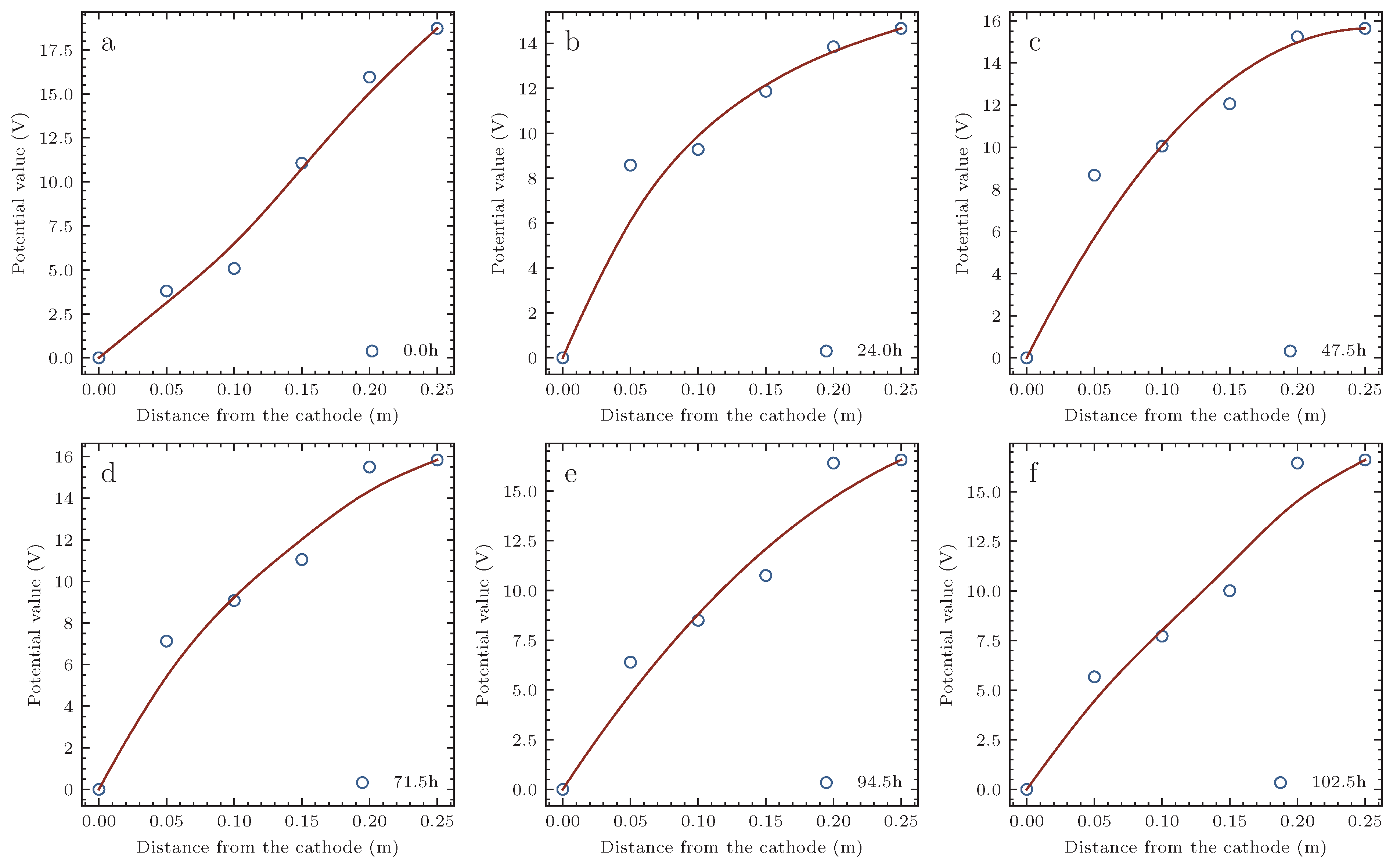
Figure 8 presents the electric potential distribution curves at six representative time instants (0 h, 24 h, 47.5 h, 71.5 h, 94.5 h, and 102.5 h) computed by PINNs. It can be seen that the adoption of the hard constraint strategy in the MLP network ensures that the boundary conditions are strictly satisfied, thereby meeting the mathematical requirements of the boundary value problem regarding the boundary conditions. At the initial moment, the electrical properties of the soil are relatively uniformly distributed, and the potential distribution is approximately linear. As electro-osmosis proceeds, the magnitudes of changes in the electrical properties of the soil at different locations exhibit differences, and the potential distribution gradually becomes distinctly nonlinear. In the later stage of electro-osmosis, most of the pore water in the soil has been expelled, the soil properties tend to become relatively homogeneous, and the potential distribution approximately returns to a linear form. The above results indicate that the independent computation by PINNs at each time instant can effectively capture the evolutionary characteristics of the potential field throughout the electro-osmotic process.
Figure 8.
Potential distribution curves at different time instants computed by PINNs. (a) 0 h, (b) 24 h, (c) 47.5 h, (d) 71.5 h, (e) 94.5 h, and (f) 102.5 h.
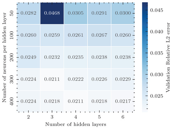
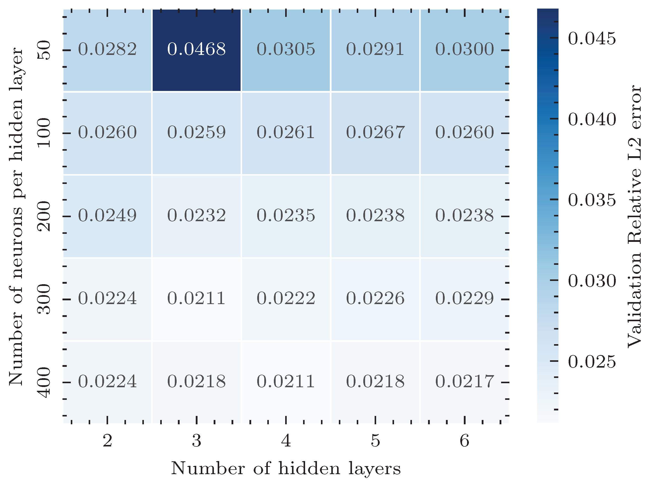
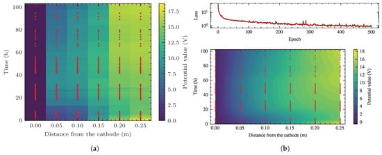
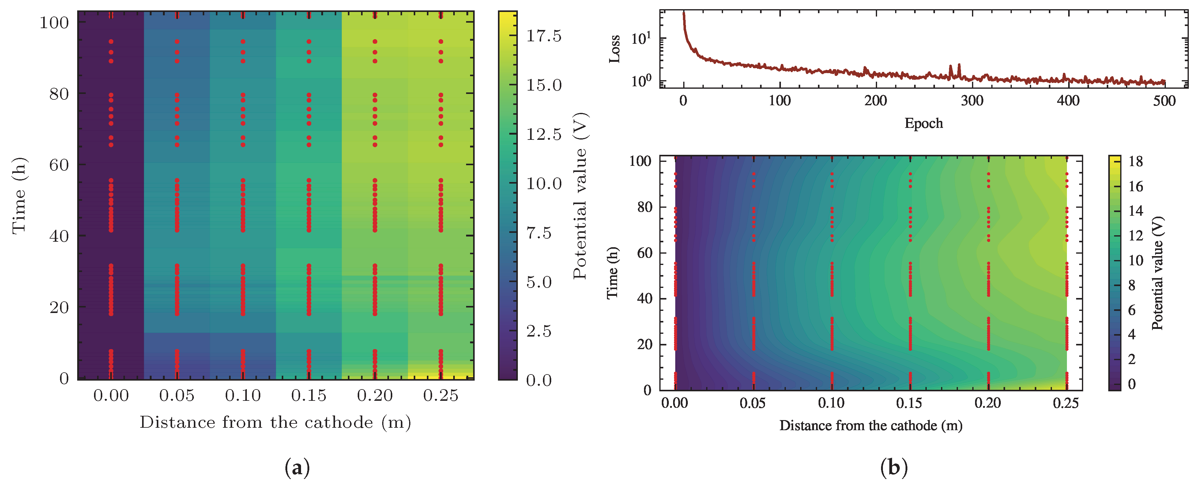
Owing to the dimensions of the model box and the occurrence of soil cracking, the number of potential monitoring points that can be installed is extremely limited; however, the sampling density in the temporal dimension can be enhanced by reducing the data acquisition interval. Based on the spatial upsampling performed by PINNs, an MLP network structure is employed to fit the spatiotemporal distribution data of the electric potential field. Figure 9 presents the results of the hyperparameter analysis in this process, through which the most reasonable network structure can be determined. For comparison, if the original monitoring data () are directly used for purely data-driven interpolation without employing PINNs for spatial densification, the results are shown in Figure 10a. It can be seen that an excessively small number of sampling points makes it difficult to accurately capture the evolutionary process of the potential field. In contrast, by employing the PINN method to densify the spatial sampling points at each time instant to 100 (), and then leveraging the fitting capability of a neural network (MLP network, 2-300-300-300-1, with ReLU activation function and MSELoss as the loss function), a spatiotemporally continuous and smooth potential function can be constructed. The training loss curve and the corresponding computational results are shown in Figure 10b. The above comparison demonstrates that the physical constraints introduced by PINNs effectively compensate for the information loss caused by sparse observations.
Figure 9.
Error heatmap of hidden layers and neuron numbers.
Figure 10.
Computed electrical potential field in the soil specimen. (a) Fitting results using raw measured potential data. (b) Training loss curve of the MLP network and the potential evolution results computed by the MLP network.
4.2. Computed Results of Excess Pore Water Pressure
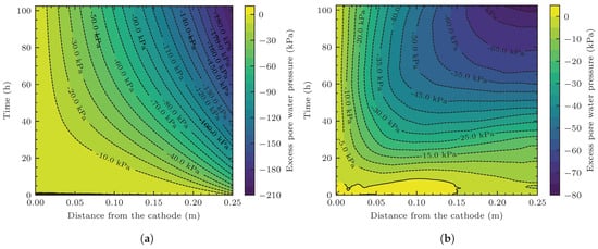
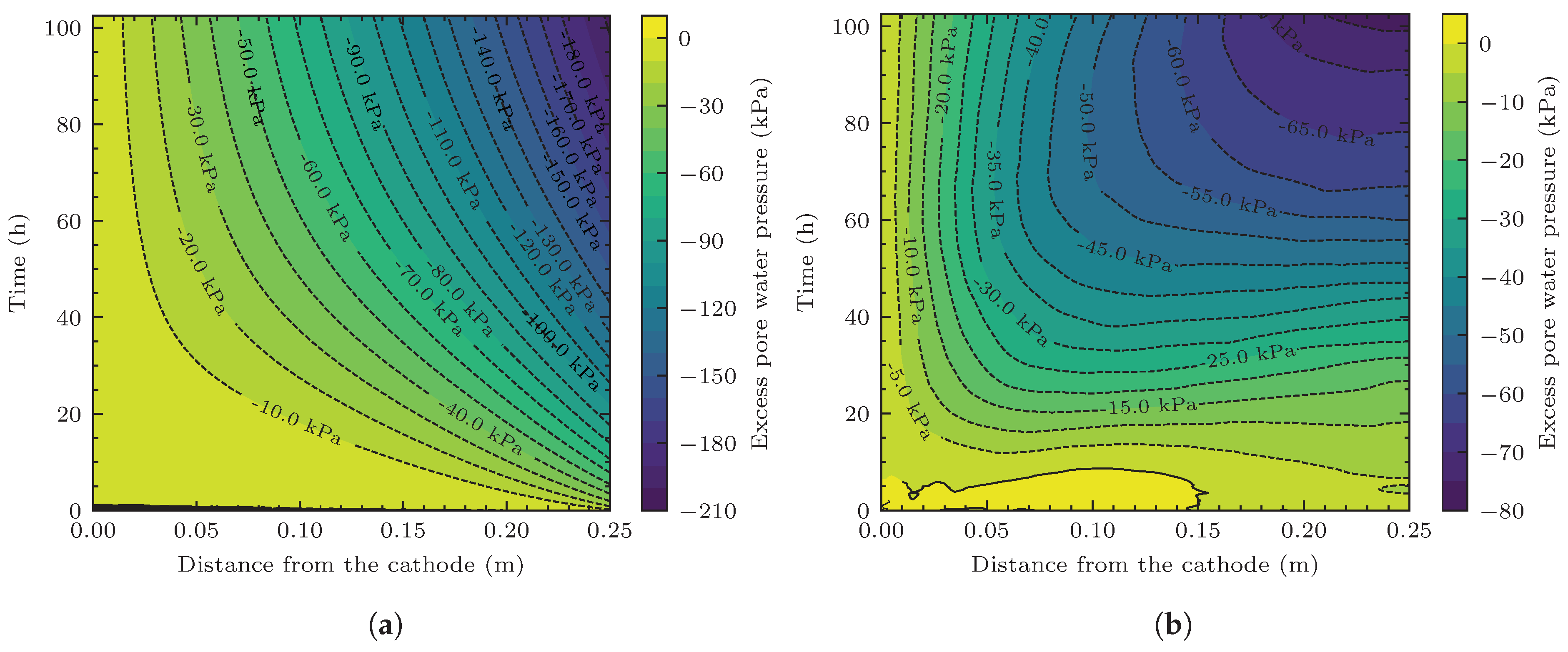
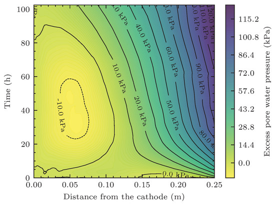
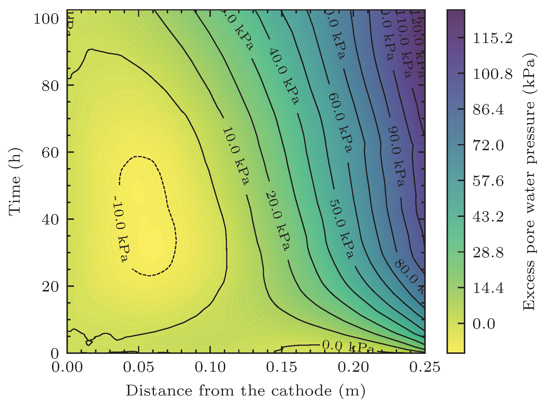
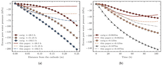
Figure 11 presents the spatiotemporal distributions of the excess pore water pressure. Specifically, Figure 11a shows the analytical results obtained from the classical theory of Esrig. This model does not account for contact voltage loss and assumes a linear distribution of the electric potential along the soil length; consequently, the calculated negative excess pore water pressures are relatively large in magnitude, with the maximum pore pressure at the anode reaching approximately kPa. Figure 11b shows the pore pressure distributions computed by the proposed method, where the maximum pore pressure magnitude is approximately kPa. Since the proposed method incorporates the experimentally measured potential distributions, the electric potential at each time instant exhibits nonlinear characteristics, and the potential gradients at different locations vary, leading to differences in the electro-osmotic driving flow velocities, which in turn result in pronounced spatial non-uniformity in the pore pressure distribution: the pore pressure variation near the anode is relatively gentle, whereas that near the cathode exhibits a higher rate of change. Figure 12 presents the deviation in pore water pressure calculation results between the two methods, i.e., the computational results of this paper minus the results of the Esrig theoretical model. It can be observed that the pore pressure magnitudes obtained from the classical theory are significantly higher than those from the proposed method near the anode, with a difference of up to approximately 120 kPa; near the cathode, however, the pore pressure magnitudes from the proposed method are slightly larger than the classical results, with a difference of approximately 10 kPa. The above comparison indicates that neglecting the nonlinear spatiotemporal evolution characteristics of the potential field significantly overestimates the development of negative pore pressure near the anode. This result has also received attention in other research literature [15,17,18].
Figure 11.
Computed contours of excess pore water pressure during electro-osmosis. (a) Pore water pressure solutions obtained from the Esrig theoretical model. (b) Pore water pressure results driven by the measured potential distribution.
Figure 12.
Deviation distribution of pore water pressure between the two models (present—Esrig).
Figure 13 further presents a comparison of pore pressures obtained by the two methods under different conditions. Specifically, Figure 13a shows the pore pressure distribution curves at different time instants. The magnitudes of negative pore pressure computed by the Esrig model are greater than those from the proposed method at all time instants, with the difference being particularly significant near the anode, and this difference tends to increase continuously with prolonged electrification time. Figure 13b presents the temporal evolution curves of pore pressure at three representative locations: near the cathode ( m), at the middle of the model ( m), and near the anode ( m). Near the cathode, the deviation between the pore pressure time-history curves of the two methods is relatively small; as the measuring point approaches the anode, the deviation gradually increases. The above results indicate that the overestimation of negative pore pressure near the anode by the classical theory accumulates and amplifies with the progress of electro-osmosis. In the proposed method, the measured potential distribution is incorporated. Combined with the potential distributions at each time instant shown in Figure 7, it can be seen that the closer to the anode during electro-osmosis, the gentler the potential gradient becomes, and the smaller the directional migration capacity of pore water. In contrast, in the classical theory, the potential field is assumed to be uniform, with a constant potential gradient, which is the primary cause of the pore pressure deviation. The actual electric potential field distribution differs significantly from the ideal state. In the application of the electro-osmotic drainage method, the influence of this variation on the soil reinforcement effect should be taken into account, with particular attention to the region near the anode. The decrease in the electric potential gradient and the occurrence of voltage loss at the anode-soil interface will, to a certain extent, weaken the soil reinforcement effect in this region. From this perspective, in the combined application of multiple methods, it would be more reasonable to adopt other methods to compensate for and mitigate the reduction in soil reinforcement effect near the anode.
Figure 13.
Spatial and temporal characteristics of pore water pressure. (a) Pore water pressure distribution curves at different time instants. (b) Pore water pressure variation curves at different positions.
4.3. Discussion on Method Characteristics
In this paper, the physics-informed neural network (PINNs) method is introduced to capture the behavior of the electric potential field during electro-osmotic consolidation. The PINNs method is employed to overcome the sparsity of measured data and enhance the descriptive capability of the spatial distribution of the electric potential field. The neural network serves as a surrogate model for the spatiotemporal evolution function of the actual electric potential field, which can directly participate as a source term in the finite difference numerical discretization of the governing equation for electro-osmotic consolidation, thereby achieving electro-osmotic consolidation calculations under actual electric potential field distributions. It should be noted that PINNs are not directly applied to the solution of pore water pressure, primarily for the following three considerations. First, in terms of solving partial differential equations, PINNs do not exhibit a clear advantage in computational efficiency and solution accuracy over conventional numerical methods (e.g., the finite difference method and the finite element method); the data-driven capability of PINNs is mainly utilized here to achieve effective integration of experimental measurement data. Second, the application of PINNs is limited to the computation of the electric potential field because potential data are relatively easy to obtain in electro-osmotic tests, whereas pore pressure transducers are relatively large in size and difficult to deploy densely, resulting in extremely limited measured data that cannot fully leverage the data-driven advantage of PINNs. Third, under ideal conditions, the potential distribution in the soil satisfies the Laplace equation; however, under the combined action of external factors (variations in the electrode-soil contact properties) and internal factors (spatiotemporal evolution of soil resistivity), the actual potential distribution deviates from linearity. The introduction of PINNs enables the synergistic use of data-driven and physical constraint (PDE residual) approaches to accurately capture the true distribution of the electric potential field. Since the potential gradient is the primary driving force for electro-osmotic flow, incorporating the measured potential distribution into the consolidation equation for pore pressure computation allows the obtained results to explain the influence of the actual electric potential field on electro-osmotic consolidation. It should be noted that during electro-osmotic consolidation, the soil consolidation caused by continuous drainage is manifested at the microscopic level as changes in the pore structure. At this point, the seepage in the porous medium does not completely follow Darcy’s law, and a nonlinear seepage relationship exists. The model in this paper is still based on the Esrig theoretical framework and is essentially a linear model, which fails to account for the nonlinear behavior of the soil permeability coefficient and volume compressibility coefficient as functions of water content or pore pressure. This is the main limitation of the present model and warrants further improvement in future studies.
5. Conclusions
In this paper, a one-dimensional electro-osmotic model test was conducted, which revealed the non-uniform evolution characteristics of soil electrical properties and the dual spatiotemporal evolution characteristics of the electric potential field. To address the computation of electro-osmotic consolidation under actual potential distributions, the PINN method was introduced to reconstruct the electric potential field at each monitoring time instant, and a multilayer perceptron (MLP) network was further adopted to construct a surrogate model for the potential field. On this basis, the surrogate model was embedded into the governing equation of electro-osmotic consolidation, and the finite difference method was employed for numerical discretization, with a dedicated computational program developed in Python. The effectiveness of the proposed method was validated through numerical examples. The main conclusions are as follows:
- The results of the one-dimensional electro-osmotic consolidation test indicate that the electric potential field does not always maintain a strictly linear distribution, but instead exhibits nonlinear characteristics as electro-osmosis proceeds, and this nonlinearity is markedly time-dependent. This is the result of the combined action of internal and external factors. In terms of internal factors, the directional migration of pore water leads to a non-uniform distribution of soil water content, which in turn causes a spatially non-uniform distribution of resistivity, causing the potential field to deviate from its initial linear state. In terms of external factors, the corrosion of metal electrodes and the volumetric shrinkage induced by soil drainage reduce the degree of electrode-soil contact, thereby decreasing the effective voltage applied across the soil. The nonlinearity of the potential distribution and its temporal evolution imply that the potential gradient is no longer constant. If this variation of the potential field is neglected, the results computed on the basis of the linear assumption will overestimate the reinforcement effect of electro-osmotic consolidation.
- The introduction of the PINN method into the computation of the electric potential field can effectively overcome the issue of sparsity in the measured data. By combining physical constraints with data-driven approaches, the actual distribution of the potential field can be well reconstructed. Furthermore, neural network fitting enables a continuous description of the evolution of the potential field in the temporal dimension, allowing the actual potential distribution information to be directly incorporated into the computation of pore water pressure. Restricting the application of PINNs to the solution of the potential field fully exploits the advantages of low-cost potential monitoring and easy data acquisition, representing a rational strategy for the involvement of PINNs in electro-osmotic consolidation problems.
- In the computation of pore water pressure, the electric potential term is treated as a non-homogeneous source term, and a finite difference scheme is directly established for numerical discretization. The surrogate model of the potential field constructed by the neural network can be embedded into the finite difference equations and participate in the iterative solution, thereby enabling accurate computation of the seepage flux driven by the actual potential gradient. Compared with the classical Esrig theory, the proposed method, which is based on measured potential data, can effectively reflect the influences of effective voltage decay and nonlinear potential field distribution on pore pressure. The computational results show that the magnitudes of negative pore pressure obtained by the new method are smaller than those from the Esrig theory, and the deviation between the two increases significantly as the anode is approached.
Author Contributions
Conceptualization, M.P. and X.Y.; Formal analysis, M.P.; Funding acquisition, M.P. and X.Y.; Investigation, X.W. and X.Z.; Methodology, M.P. and X.Y.; Project administration, X.Y.; Resources, X.W.; Software, X.Y.; Supervision, X.W.; Validation, M.P. and X.Z.; Visualization, X.Z.; Data curation, X.W.; Writing—original draft, M.P.; Writing—review & editing, X.W. and X.Y. All authors have read and agreed to the published version of the manuscript.
Funding
This research was funded by the Natural Science Foundation of Gansu Province (Grant No. 26JRRA680), the Scientific Research Project of the Education Department of Gansu Province (Grant No. 2025B-245), the Enterprise Technology Demand Project of Gansu Chemical Industry Research Institute (Grant No. 2025GH-08), the 2025 University-Level Research and Innovation Team, Lanzhou Petrochemical University of Vocational Technology (Grant No. 004).
Institutional Review Board Statement
Not applicable.
Informed Consent Statement
Not applicable.
Data Availability Statement
The data supporting the reported results is available from the corresponding author on request.
Conflicts of Interest
The authors declare no conflicts of interest.
Abbreviations
The following abbreviations are used in this manuscript:
| PINN | Physics-informed neural network |
| DC | Direct Current |
| PDE | Partial differential equation |
| FDM | Finite difference method |
| MLP | Multilayer perceptron |
| MSE | Mean squared error |
References
- Casagrande, I.L. Electro-Osmosis in Soils. Géotechnique 1949, 1, 159–177. [Google Scholar] [CrossRef] [Scilit]
- Wan, T.Y.; Mitchell, J.K. Electro-Osmotic Consolidation of Soils. J. Geotech. Eng. Div. 1976, 102, 473–491. [Google Scholar] [CrossRef] [Scilit]
- Mitchell, J.K. Conduction phenomena: From theory to geotechnical practice. Géotechnique 1991, 41, 299–340. [Google Scholar] [CrossRef] [Scilit]
- Bjerrum, L.; Moum, J.; Eide, O. Application of Electro-Osmosis to a Foundation Problem in a Norwegian Quick Clay. Géotechnique 1967, 17, 214–235. [Google Scholar] [CrossRef] [Scilit]
- Esrig, M.I. Pore Pressures, Consolidation, and Electrokinetics. J. Soil Mech. Found. Div. 1968, 94, 899–921. [Google Scholar] [CrossRef] [Scilit]
- Lewis, R.W.; Humpheson, C. Numerical Analysis of Electro-Osmotic Flow in Soils. J. Soil Mech. Found. Div. 1973, 99, 603–616. [Google Scholar] [CrossRef] [Scilit]
- Yuan, J.; Hicks, M.A. Large deformation elastic electro-osmosis consolidation of clays. Comput. Geotech. 2013, 54, 60–68. [Google Scholar] [CrossRef] [Scilit]
- Zhou, Y.; Deng, A.; Wang, C. Finite-difference model for one-dimensional electro-osmotic consolidation. Comput. Geotech. 2013, 54, 152–165. [Google Scholar] [CrossRef] [Scilit]
- Deng, A.; Zhou, Y. Modeling Electroosmosis and Surcharge Preloading Consolidation. II: Validation and Simulation Results. J. Geotech. Geoenviron. Eng. 2016, 142, 04015094. [Google Scholar] [CrossRef] [Scilit]
- Wu, H.; Qi, W.; Hu, L.; Wen, Q. Electro-osmotic consolidation of soil with variable compressibility, hydraulic conductivity and electro-osmosis conductivity. Comput. Geotech. 2017, 85, 126–138. [Google Scholar] [CrossRef] [Scilit]
- Wang, L.; Huang, P.; Liu, S.; Alonso, E. Analytical solution for nonlinear consolidation of combined electroosmosis-vacuum-surcharge preloading. Comput. Geotech. 2020, 121, 103484. [Google Scholar] [CrossRef] [Scilit]
- Jiang, W.; Ge, S.; Huang, X.; Chen, Z.; Li, J. General analytical solutions for one-dimensional large strain consolidation of soft soils under electro-osmosis-surcharge preloading. Soils Found. 2022, 62, 101211. [Google Scholar] [CrossRef] [Scilit]
- Zhou, Y.; Zhang, S.; Feng, S.; Deng, A. One-dimensional large strain electro-osmotic consolidation model based on multi-field coupling. Comput. Geotech. 2023, 159, 105491. [Google Scholar] [CrossRef] [Scilit]
- Zhou, J.; Gan, Q.; Tao, Y. Electro-osmotic permeability model based on ions migration. Acta Geotech. 2022, 17, 2379–2393. [Google Scholar] [CrossRef] [Scilit]
- Feng, J.; Shen, Y.; Liu, H.; Shi, W. An analytical solution of electroosmotic consolidation concerning effective voltage attenuation. Acta Geotech. 2023, 18, 1169–1177. [Google Scholar] [CrossRef] [Scilit]
- Yang, X.; Pei, M.; Xie, Y.; Zhou, X.; Dong, X. Experimental and Numerical Investigation of One-Dimensional Electroosmotic Consolidation Based on Segment Inheritance Strategy. Adv. Civ. Eng. 2024, 2024, 7917994. [Google Scholar] [CrossRef] [Scilit]
- Shen, Y.; Feng, J.; Ma, Y.; Liu, H. Two-Dimensional Electroosmotic Consolidation Theory of Nonlinear Soil Voltage Distribution Characteristics. Adv. Civ. Eng. 2019, 2019, 7354873. [Google Scholar] [CrossRef] [Scilit]
- Feng, J.; Shen, Y.; Xu, J.; Shi, W. Analytical solution of vacuum preloading technology combined with electroosmosis coupling considering impacts of distribution of soil’s electrical potential. J. Cent. South Univ. 2021, 28, 2544–2555. [Google Scholar] [CrossRef] [Scilit]
- Zhao, X.; Min, J.; Ding, S.; Liu, Y.; Liao, J.; Zhang, S. Analytical Solution for 2D Electro-Osmotic Consolidation of Unsaturated Soil With Non-linear Voltage Distribution. Int. J. Numer. Anal. Methods Geomech. 2024, 48, 4457–4468. [Google Scholar] [CrossRef] [Scilit]
- Zhao, X.D.; Liu, Y.; Gong, W.H. Analytical solution for one-dimensional electro-osmotic consolidation of double-layered system. Comput. Geotech. 2020, 122, 103496. [Google Scholar] [CrossRef] [Scilit]
- Chen, Z.L.; Li, J.P.; Xu, Y.S.; Liu, J.; Wang, S. Effect of soil layering and interface resistance on electro-osmotic consolidation of layered soils: A Green’s function approach. Int. J. Numer. Anal. Methods Geomech. 2024, 48, 2880–2899. [Google Scholar] [CrossRef] [Scilit]
- Chen, Z.L.; Li, J.P.; Luo, Z.Y.; Wang, Y.; Xu, Y.S. A two-dimensional analytical solution for electro-osmotic consolidation in multi-layered soft soils using vertical electrodes. Can. Geotech. J. 2025, 62, 1–19. [Google Scholar] [CrossRef] [Scilit]
- Li, J.P.; Luo, W.D.; Chen, Z.L.; Liu, J.; Wang, S. Effect of permeable anode on electroosmotic consolidation using the horizontal electro-kinetic geosynthetics: Analytical approach. Acta Geotech. 2024, 19, 6289–6304. [Google Scholar] [CrossRef] [Scilit]
- Liu, Y.; Zheng, J.J.; Zhao, X.; Cao, W.; Huang, Z. A closed-form solution for axisymmetric electro-osmotic consolidation considering smear effects. Acta Geotech. 2022, 17, 2597–2609. [Google Scholar] [CrossRef] [Scilit]
- Zong, M.; Li, L.; Wu, W.; Zhang, Y.; Mei, G. Analytical Solution for Radial Consolidation of Combined Electroosmotic, Vacuum, and Surcharge Preloading Considering Smear Effects. Int. J. Geomech. 2024, 24, 04024141. [Google Scholar] [CrossRef] [Scilit]
- Wang, L.; Wang, Y.; Liu, S.; Fu, Z.; Shen, C.; Yuan, W. Analytical solution for one-dimensional vertical electro-osmotic drainage under unsaturated conditions. Comput. Geotech. 2019, 105, 27–36. [Google Scholar] [CrossRef] [Scilit]
- Wang, L.J.; Wang, Y.M.; Liu, S.H.; Huang, P.H. Analytical Investigation of Electroosmotic Consolidation in Unsaturated Soils Considering the Coupling Effect and a Nonuniform Initial Water Content. Int. J. Geomech. 2021, 21, 06021018. [Google Scholar] [CrossRef] [Scilit]
- Liu, Y.; Zheng, J.J.; Zhao, X.; You, L. Analytical model for two-dimensional electro-osmosis-enhanced preloading consolidation of unsaturated soil. Acta Geotech. 2023, 18, 1093–1110. [Google Scholar] [CrossRef] [Scilit]
- Zhao, X.; Ni, J.; Liu, Y.; Gong, W. A general analytical solution for axisymmetric electro-osmotic consolidation of unsaturated soil with semi-permeable boundary. Int. J. Numer. Anal. Methods Geomech. 2024, 48, 2542–2563. [Google Scholar] [CrossRef] [Scilit]
- Jiang, L.; Qin, A.; Li, L.; Meng, H. Analytical solution of electroosmotic-surcharge preloading coupled consolidation for unsaturated soil via Electric Prefabricated Vertical Drains (EVDs). Transp. Geotech. 2023, 42, 101088. [Google Scholar] [CrossRef] [Scilit]
- Jiang, L.; Qin, A.; Li, L. The role of free-strain assumption in axisymmetric electro-osmosis-enhanced preloading consolidation of unsaturated soil. Int. J. Numer. Anal. Methods Geomech. 2023, 47, 2493–2510. [Google Scholar] [CrossRef] [Scilit]
- Meng, H.; Qin, A.; Jiang, L.; Li, L. General Semianalytical Solution for Axisymmetric Consolidation of Unsaturated Soil with Unified Boundary under Electroosmotic and Surcharge Preloading. J. Eng. Mech. 2023, 149, 04023091. [Google Scholar] [CrossRef] [Scilit]
- Zhang, J.; Zong, M.; Wu, W.; Zhang, Y.; Mei, G. Analytical solution for radial consolidation of combined electroosmosis-vacuum-surcharge preloading considering free strain and cyclic loading. Comput. Geotech. 2024, 176, 106810. [Google Scholar] [CrossRef] [Scilit]
- Lu, X.; Li, C.; Wang, P. An analytical solution for the nonlinear large strain consolidation of soils treated by electro-osmosis combined with vacuum and surcharge preloading. Comput. Geotech. 2024, 174, 106620. [Google Scholar] [CrossRef] [Scilit]
- Zhang, L.; Hou, F.; Chen, Y.; Lv, Y.; Wang, B.; Jin, D.; Fang, C.; Wang, L. Two-Dimensional Analytical Solutions for Marine Clay Consolidation Under Coupled Electro-Osmosis, Surcharge, and Vacuum Preloading with Radial-Vertical Attenuation. Int. J. Numer. Anal. Methods Geomech. 2026, 50, 502–518. [Google Scholar] [CrossRef] [Scilit]
- Ge, S.; Jiang, W.; Wang, J.P.; Feng, G.; Zheng, L.; Xie, X. Coupled model for electro-osmosis consolidation and ion transport considering chemical osmosis in saturated clay soils. Int. J. Numer. Anal. Methods Geomech. 2024, 48, 3455–3474. [Google Scholar] [CrossRef] [Scilit]
- Qi, W.; Shen, Y.; Li, S.; Chen, K.; Xu, J. Simultaneous consolidation and remediation of copper-contaminated sediments with vacuum electro-osmosis. Can. Geotech. J. 2025, 62, 1–11. [Google Scholar] [CrossRef] [Scilit]
- Jin, D.; Zhang, H.; Zhang, Z.; Wang, Z.; Zhang, Y. Multi-Physical Response and Directional Cation-Moisture Migration in Frozen Clay under Saline Electro-Osmosis. Cold Reg. Sci. Technol. 2026, 244, 104815. [Google Scholar] [CrossRef] [Scilit]
- Sun, X.; Zhang, R.; Wang, Y.; Jin, X.; Yu, Q. A novel evaluation method of consolidation efficiency of electro-osmotic system. Géotechnique 2024, 74, 1421–1430. [Google Scholar] [CrossRef] [Scilit]
- Zhang, X.; Zheng, L.; Ge, S.; Zheng, X.; Xie, X. Electroosmotic reinforcement mechanism and laboratory tests of pulsating direct current with a high energy efficiency ratio. Soils Found. 2024, 64, 101423. [Google Scholar] [CrossRef] [Scilit]
- Wu, H.; Hu, L.; Wen, Q. Numerical Assessment of Equivalent Radius for Electrokinetic Geosynthetics Electrodes during Electroosmotic Consolidation. Int. J. Geomech. 2018, 18, 04018024. [Google Scholar] [CrossRef] [Scilit]
- Yang, X.; Xie, Y.; Dong, J.; Liu, G.; Zheng, Y. Study on Electroosmosis Consolidation of Punctiform Electrode Unit. Adv. Mater. Sci. Eng. 2021, 2021, 6627331. [Google Scholar] [CrossRef] [Scilit]
- Raissi, M.; Perdikaris, P.; Karniadakis, G.E. Physics-informed neural networks: A deep learning framework for solving forward and inverse problems involving nonlinear partial differential equations. J. Comput. Phys. 2019, 378, 686–707. [Google Scholar] [CrossRef] [Scilit]
- Raissi, M.; Yazdani, A.; Karniadakis, G.E. Hidden fluid mechanics: Learning velocity and pressure fields from flow visualizations. Science 2020, 367, 1026–1030. [Google Scholar] [CrossRef] [Scilit]
- Karniadakis, G.E.; Kevrekidis, I.G.; Lu, L.; Perdikaris, P.; Wang, S.; Yang, L. Physics-informed machine learning. Nat. Rev. Phys. 2021, 3, 422–440. [Google Scholar] [CrossRef] [Scilit]
- Li, H.; Miao, Y.; Khodaei, Z.S.; Aliabadi, M.H. Finite-PINN: A physics-informed neural network with finite geometric encoding for solid mechanics. J. Mech. Phys. Solids 2025, 203, 106222. [Google Scholar] [CrossRef] [Scilit]
- Liu, M.; Zhang, Q.; Fuentes, R. A FEM-PINN approach to modelling elastoplastic soil behaviour in boundary value problems. Comput. Geotech. 2026, 190, 107761. [Google Scholar] [CrossRef] [Scilit]
- Wu, J.; Zhao, W.; Wang, K.; Naggar, M.H.E. Physics-informed neural networks (PINNs) for dynamic pile-soil interaction problems. Comput. Geotech. 2026, 193, 107941. [Google Scholar] [CrossRef] [Scilit]
- Samaniego, E.; Anitescu, C.; Goswami, S.; Nguyen-Thanh, V.M.; Guo, H.; Hamdia, K.; Zhuang, X.; Rabczuk, T. An energy approach to the solution of partial differential equations in computational mechanics via machine learning: Concepts, implementation and applications. Comput. Methods Appl. Mech. Eng. 2020, 362, 112790. [Google Scholar] [CrossRef] [Scilit]
- Rezaei, S.; Asl, R.N.; Taghikhani, K.; Moeineddin, A.; Kaliske, M.; Apel, M. Finite Operator Learning: Bridging neural operators and numerical methods for efficient parametric solution and optimization of PDEs. Finite Elem. Anal. Des. 2026, 254, 104506. [Google Scholar] [CrossRef] [Scilit]
- Asgarkhani, N.; Kazemi, F.; Jankowski, R. Machine-learning based tool for seismic response assessment of steel structures including masonry infill walls and soil-foundation-structure interaction. Comput. Struct. 2025, 317, 107918. [Google Scholar] [CrossRef] [Scilit]

Disclaimer/Publisher’s Note: The statements, opinions and data contained in all publications are solely those of the individual author(s) and contributor(s) and not of MDPI and/or the editor(s). MDPI and/or the editor(s) disclaim responsibility for any injury to people or property resulting from any ideas, methods, instructions or products referred to in the content. |
© 2026 by the authors. Licensee MDPI, Basel, Switzerland. This article is an open access article distributed under the terms and conditions of the Creative Commons Attribution (CC BY) license.