


Featured Application
Low-cost acoustic sensing for identifying paired-object combinations hidden from direct view, relevant to security screening, search and rescue, and indoor autonomous navigation.
Abstract
Detecting and identifying objects outside the direct line of sight is important for security, search and rescue, and autonomous systems, and acoustic sensing offers a low-cost and environmentally robust alternative to optical non-line-of-sight (NLOS) methods. Most acoustic NLOS studies address a single object. This study addresses the classification of paired object combinations from secondary NLOS acoustic reflections. Linear chirp signals reflected from a wall were recorded with an eight-loudspeaker, eight-microphone array in a single controlled room (120 recordings, four balanced classes). A fixed-size, 513-dimensional short-time Fourier-transform (STFT) spectral summary was classified with Random Forest, Decision Tree, k-Nearest Neighbors, and Multilayer Perceptron models using recording-level stratified five-fold cross-validation repeated over five seeds. Random Forest and the Multilayer Perceptron reached accuracies of 0.9850 ± 0.0207 and 0.9600 ± 0.0231, respectively, against a chance level of 0.25. Comparisons with MFCC, Welch, and compact spectral-descriptor representations, single-microphone and multi-channel strategies, and preprocessing ablations, together with label-permutation and nuisance-baseline controls, indicate that the separation is carried by the spectral envelope rather than by gross amplitude, and that the eight-channel array gave no systematic advantage over a single microphone in this dataset. The results are limited to one room, one reflective surface, and recording-level evaluation, and they do not demonstrate generalization to unseen sessions or rooms.
1. Introduction
Detecting objects and identifying their types in non-line-of-sight (NLOS) environments remains an open problem in applications such as security, search and rescue, autonomous driving, and indoor sensing. In scenarios where the direct line of sight is blocked by a wall, corner, or partition, information about the target can be obtained only through indirect components reflected from surrounding surfaces. Under such conditions, conventional imaging systems fail because they cannot establish a direct path to the target, so reflection-based sensing is required [1,2].
Optics-based NLOS methods address this problem through the temporal and spatial analysis of light reflections. Velten et al. [3] reconstructed the three-dimensional geometry of objects located around a corner using an ultrafast time-of-flight technique; O’Toole et al. [2] proposed a confocal imaging model based on the light-cone transform; and Heide et al. [4] developed a reconstruction framework that accounts for partial occluders and surface normals. Although these approaches provide high spatial resolution, they require complex and expensive hardware such as femtosecond laser sources and single-photon detectors; moreover, because they are sensitive to environmental factors such as dust, smoke, and varying illumination, they impose a requirement for controlled environments.
Radiofrequency (RF) and radar-based methods, in turn, exploit the multipath propagation characteristics of electromagnetic waves to classify and track moving targets around corners [5]. Although these systems offer the advantage of illumination-independent operation, they suffer from drawbacks such as the need for wideband antenna arrays and dedicated hardware, regulatory constraints, and limited discrimination capability for small or weakly reflecting targets; their capacity to produce material-specific discriminative information is also comparatively limited. These limitations have strengthened interest in sensing modalities that are low-cost and environmentally robust.
In this context, acoustics-based NLOS sensing is an attractive low-cost alternative. In addition to offering low hardware cost, portability, and low energy consumption, sound waves are far less affected by dust, smoke, and variations in lighting conditions than optical systems. Lindell et al. [1] introduced a pioneering framework for NLOS imaging with acoustic signals; Bianco et al. [6] reviewed the potential of machine learning-assisted acoustic systems across a broad application spectrum, including object detection, localization, and recognition. Schulz et al. [7] experimentally demonstrated that vehicles located around a corner can be detected through acoustic reflections, and Boger-Lombard et al. [8] addressed passive acoustic localization using uncontrolled noise sources. With respect to classification, Xu et al. [9] showed that acoustic NLOS signals can be recognized by a convolutional neural network equipped with a channel-attention mechanism. Collectively, these studies confirm that acoustic reflections carry discriminative spectral signatures related to the material and geometry of the object.
In the acoustic setting considered here, the propagation path can be summarized as follows. A loudspeaker array emits a wideband chirp toward a reflective wall; the wall redirects part of the sound toward the hidden objects behind a barrier; the objects reflect and scatter part of this energy back toward the wall; and the wall returns it to the microphones. The first arrival is the strong primary reflection from the wall, and the delayed and weaker component that follows is the secondary reflection, which carries the object-dependent spectral information exploited in this study.
Nevertheless, the vast majority of the acoustic NLOS literature remains confined to detecting the mere presence of a target, estimating its position, or classifying a single object or material type. Closely related prior studies likewise reflect this tendency: the classification of single object types from multi-channel acoustic reflections [10], the estimation of the position of an object in the NLOS region using acoustic signals [11], and single-material recognition combining wavelet–acoustic hybrid features with deep recurrent networks [12] may be regarded as falling within this scope. All of these studies focus on scenarios containing a single target in the environment.
Real-world environments, however, typically contain several objects simultaneously. The secondary reflections generated by several objects overlap in the time–frequency plane, producing superimposed and considerably more complex spectral patterns, which makes the discrimination problem substantially harder than in the single-target case. Whether multi-object combinations can be learned and discriminated solely from secondary acoustic reflections remains a largely open problem. This constitutes the first gap addressed here.
A second gap concerns the interpretation of high accuracies on small acoustic NLOS datasets. Such datasets typically consist of repeated measurements acquired with the same physical setup, so that recording-level cross-validation quantifies the separability of the available recordings rather than generalization to new scenes, and a single random split can overstate or understate performance. High reported accuracy therefore needs to be accompanied by controls (repeated seeds, label permutation, trivial baselines, ablations of the feature representation, and an explicit statement of what the validation protocol does and does not show).
This study addresses both gaps. It classifies paired object combinations under NLOS conditions from secondary acoustic reflections and evaluates the classifiers with a recording-level, multi-seed protocol accompanied by explicit controls. A multi-channel acoustic setup consisting of eight loudspeakers and eight microphones is used to acquire the data; linear chirp signals generated in the 2–20 kHz range are transmitted toward a wall serving as the reflective surface, and, following the primary reflections returning from the surface, the secondary components reflected indirectly from the object combinations located in the NLOS region are isolated. The eight array channels are averaged into a single-channel signal, from which a compact, fixed-size STFT-based spectral summary is extracted; this deliberately compact representation is then evaluated with Random Forest, k-Nearest Neighbors, Decision Tree, and Multilayer Perceptron classifiers. Beyond this baseline, the study examines whether the STFT summary is actually needed (comparison with MFCC, Welch, and compact spectral-descriptor representations), whether the eight-microphone array contributes beyond a single microphone (single-microphone, channel-statistics, and feature-concatenation strategies), and whether the result is explained by trivial factors (label permutation, a nuisance baseline, and preprocessing ablations). Compared with the closest recent work on material classification from acoustic NLOS echoes [12], which addresses nine single materials with a hybrid wavelet–acoustic representation and recurrent networks, the specific unresolved question addressed here is whether two co-located objects, whose secondary reflections overlap in the time–frequency plane, can be separated from the reflection spectrum alone, and which representation and channel strategy are actually needed to do so. The classification results are examined through per-class metrics, pooled confusion patterns, and class-mean spectral profiles. The results were obtained with a basic feature representation, and the dataset was collected in a single environment.
The principal contributions of this study are as follows:
- A paired-object NLOS classification problem is formulated, and a labeled dataset of 120 recordings of four paired (two-object) combinations is compiled with file-schema-based labeling and repeated measurements for each class;
- A compact, reproducible STFT spectral-summary representation is derived from the array-averaged signal and is benchmarked against MFCC, Welch-spectrum, and compact spectral-descriptor representations, showing that detailed frequency-domain information (STFT and Welch) is what separates the classes;
- A recording-level, multi-seed (five seeds, 25 fold evaluations per configuration) cross-validation protocol is adopted, with identical folds shared across classifiers, representations, preprocessing ablations, and channel strategies, so that all comparisons are paired, and the reported standard deviations reflect stability across seeds;
- The high accuracy is examined with label-permutation testing, a nuisance baseline, preprocessing ablations, and a systematic comparison of single-microphone and multi-channel strategies; the analysis shows that the separation is not explained by gross amplitude or chance, and that the eight-channel array provides no systematic gain over a single microphone in this dataset.
2. Related Work
Approaches to the problem of target detection under NLOS conditions can largely be grouped, according to the carrier signal they employ, into optical, radiofrequency/radar-based, and acoustic methods. Their common denominator is that, in the absence of a direct line of sight, they extract information about the target by analyzing indirect components reflected from surfaces; they differ in resolution, hardware cost, environmental robustness, and the type of information they produce (presence, position, or object/material class).
Optics-based methods have provided the highest spatial resolution in NLOS imaging. Velten et al. [3] succeeded in recovering the three-dimensional geometry of objects around a corner using ultrafast time-of-flight measurements; however, because the method relies on femtosecond lasers and extremely precise timing hardware, it entails a cost that limits its practical use. Although O’Toole et al. [2] shortened the reconstruction time with a confocal formulation based on the light-cone transform, the method still depends on controlled lighting conditions and specialized scanning setups. Heide et al. [4] moved closer to realistic scenes by incorporating partial occluders and surface normals into the model, and Isogawa et al. [13] addressed out-of-sight human pose estimation within a physics-based framework. Next-generation deep-learning-based methods have aimed to reduce the computational burden in this field: Zhu and Cai [14] proposed fast NLOS imaging via two-step deep remapping, and Shen et al. [15] improved image quality through neural transient fields. Although these studies are strong in terms of resolution, their sensitivity to dust, smoke, and illumination changes, together with their high hardware requirements, continues to constitute a significant constraint for low-cost systems that are robust under field conditions. Another branch of the optical family uses passive image cues instead of active laser setups: Naser et al. [16] proposed an infrastructure-free system (“ShadowCam”) that detects out-of-sight obstacles for autonomous vehicles by tracking ground-reflected shadows and faint illumination changes with a camera; although the method is low-cost, it depends on sufficient illumination and suitable scene geometry and produces no information about the material type of the target.
Radiofrequency/radar-based methods, in turn, constitute a separate and well-established line of work. Scheiner et al. [5] were able to classify and track moving targets around corners in real field conditions using Doppler radar measurements; although such approaches operate independently of illumination, they entail constraints such as the need for dedicated hardware and wide bandwidth, as well as limited discrimination capability for small or weakly reflecting targets. These limitations strengthen interest in the acoustic modality, both in terms of hardware simplicity and material-sensitive reflection characteristics.
In the acoustic case, the same principle is realized with sound: a wideband signal is sent toward a reflective surface, the surface redirects it toward the hidden scene, and the weak, delayed echo that returns along the indirect path carries object-dependent spectral information.
A significant portion of the acoustic NLOS literature has concentrated on imaging the target, detecting its presence, or estimating its position. Lindell et al. [1] introduced a pioneering framework for NLOS imaging with acoustic waves, showing that sound reflected from a wall can be used to reconstruct the out-of-sight scene; Shin et al. [17] improved acoustic NLOS imaging quality through cross-modal knowledge distillation. Along the localization axis, Boger-Lombard et al. [8] estimated the position of a target around a corner with a passive acoustic approach that uses uncontrolled noise sources, and Zhang et al. [18] improved indoor localization accuracy by discriminating LOS from NLOS conditions on the basis of acoustic channel characteristics. In presence detection, Schulz et al. [7] demonstrated that the sound reflections produced by vehicles located around a corner can be reliably detected with machine learning. Although these studies demonstrate that acoustic reflections contain valuable information for NLOS sensing, their outputs are largely confined to determining whether a target is present or where it is located. They do not address the identification of the target itself, such as its material composition or object type.
Acoustic NLOS studies focusing on object and material classification are comparatively more recent and are generally restricted to scenarios containing a single target. Xu et al. [9] achieved high accuracy by recognizing acoustic NLOS signals with a one-dimensional convolutional neural network equipped with a channel-attention mechanism; however, the evaluation was again conducted within a single-target setting. The comprehensive review presented by Bianco et al. [6] documents in a holistic manner the potential of machine learning-assisted acoustic systems for such tasks. Although these classification-oriented studies are valuable, they draw their inferences from single targets and leave out of scope the scenarios in which several objects are present together, and the reflections consequently overlap.
Closely related acoustic NLOS studies also reflect this single-target tendency. Çalışan et al. [10] extracted MFCC features from secondary reflections collected with a multi-channel setup comprising eight loudspeakers and eight microphones and classified single object types such as wood, iron, brick, PVC, and household appliances using Decision Tree, k-NN, and MLP, with the highest performance attained by the Decision Tree; however, the study is limited to single-object scenarios and a relatively small sample. Olgun and Çalışan [11] focused on estimating the position of an object in the NLOS region with a similar acoustic setup and did not address object-type discrimination. In a related study [19], reflections collected with an identical multi-channel setup were evaluated for liveness discrimination; the raw multi-channel representation, arithmetic averaging, and learned latent fusion strategies were compared across different classifier inductive biases. Although this study provides presence-level discrimination, it does not include the type-based discrimination of co-located multi-object combinations. Alakuş and Türkoğlu [12], in turn, proposed a 70-dimensional hybrid representation that combines multi-scale energy–entropy statistics derived from ten different wavelet families with classical acoustic features such as MFCC, RMS, and ZCR; training this representation with LSTM, BiLSTM, GRU, BiGRU, and CNN-LSTM architectures, they obtained high accuracy across nine material classes. Although this study offers a strong contribution in terms of feature fusion, it remains limited to single-material classification, whereas the present study addresses paired-object combinations whose reflections overlap and complements this with explicit representation, channel-strategy, and control analyses.
This study differs from previous work in three principal respects. First, it goes beyond the presence-detection, localization, and single-object/material-classification problems on which the existing acoustic NLOS literature has focused, and instead discriminates multi-object combinations containing several co-located objects solely from secondary acoustic reflections. Second, the complex spectral patterns formed by overlapping reflections are modeled with a computationally lightweight, fixed-size STFT-based summary representation, preserving a low-cost and interpretable framework. Third, the high accuracy is not taken at face value: the evaluation uses recording-level cross-validation repeated over five seeds with identical folds across all comparisons, and it is accompanied by feature-representation, channel-strategy, and preprocessing ablations, label-permutation testing, and a nuisance baseline, while stating explicitly that recording-level validation measures separability within the dataset and not generalization to unseen sessions or rooms. A comparative summary of the reviewed studies is presented in Table 1.
Table 1.
Comparison of selected studies conducted in NLOS environments in terms of modality, task, method, and principal limitation.
3. Materials and Methods
This section presents the end-to-end framework designed for classifying paired object combinations from secondary acoustic reflections under NLOS conditions. The process comprises the following steps: establishing the experimental data acquisition setup (Section 3.1), constructing the labeled dataset (Section 3.2), isolating the secondary reflections and preprocessing the signals (Section 3.3), spectral feature representations and multi-channel strategies (Section 3.4), classification models and the evaluation protocol (Section 3.5), and performance metrics and statistical reporting (Section 3.6). The overall workflow of the proposed method is shown in Figure 1. Beginning with multi-channel NLOS acoustic measurements, the process applies preprocessing steps such as secondary-reflection isolation, pre-emphasis, and normalization. Spectral features are obtained from the preprocessed single-channel signal using short-time Fourier transform (STFT), where the eight microphone channels are first combined at the sample level to form a fixed-size feature representation [20]. The resulting features are classified with Random Forest [21], k-Nearest Neighbors (k-NN) [22], Decision Tree [23], and Multilayer Perceptron (MLP) [24] models. Alternative representations and channel strategies are evaluated in addition to this baseline. Model performance is evaluated with recording-level stratified five-fold cross-validation repeated over five seeds, and the results are analyzed in terms of classification performance, control experiments, and physical interpretation.
Figure 1.
Overall workflow of the proposed NLOS acoustic paired-object classification framework.
The computational procedures were implemented using Python (version 3.13.11; Python Software Foundation), NumPy (version 2.3.5), and TensorFlow (version 2.20.0; Google).
3.1. Experimental Setup
In order to collect the acoustic reflections of object combinations located outside the line of sight, a multi-channel acoustic data acquisition system consisting of eight loudspeakers and eight measurement microphones was designed. The loudspeakers and microphones were positioned sequentially and coplanarly on a vertical carrier panel; the loudspeakers were directed toward a rigid wall serving as the reflective surface, while the microphones were aligned in the same plane, parallel to the loudspeakers, so as to capture reflections returning both from the surface and from the objects in the NLOS region. The schematic structure of the proposed multi-channel NLOS acoustic data acquisition system and the signal propagation mechanism are shown in Figure 2. This multi-channel layout allows each generated excitation signal to be recorded simultaneously by the eight microphones. The data acquisition process was carried out in a dedicated non-line-of-sight analysis laboratory established for this purpose, under controlled conditions with acoustic and optical isolation. The actual experimental setup in the established laboratory environment is presented in Figure 3.
Figure 2.
Schematic representation of the proposed multi-channel NLOS acoustic data acquisition system and the signal propagation mechanism.
Figure 3.
Non-line-of-sight analysis laboratory and multi-channel acoustic data acquisition setup: (a) the data acquisition station and the NLOS compartment in which the direct line of sight is obstructed; (b) close-up view of the vertical panel carrying the eight loudspeakers and eight measurement microphones.
Room and array geometry: The top view of the experimental room is shown in Figure 4. The room measures 2.6 m × 3.0 m. The experimental equipment is located on one side of a barrier wall (200 cm × 200 cm, 30 cm thick), whereas the hidden objects are placed on the other side, in the NLOS area, so that no direct path exists between the array and the objects. A reflective surface (100 cm × 200 cm) is mounted on the far wall, 45 cm beyond the end of the barrier wall, and the experimental equipment is located 120 cm from this surface. The hidden object pair (material pair) was placed within a region extending 110 cm from the barrier wall. A partition wall (160 cm × 200 cm) separates the measurement area from the entrance, and the room boundaries are lined with glass-wool insulated panels and a blackout curtain.
Figure 4.
Top view of the experimental room, showing the barrier wall, the reflective surface, the experimental equipment, and the NLOS area containing the hidden object pair (dimensions in cm or m as labeled).
The acoustic sensor array is shown in Figure 5. The vertical panel is 80 cm high and 10 cm wide and carries eight loudspeakers (T1–T8) and eight measurement microphones (Mic 1–Mic 8) with a microphone spacing of 10 cm; the panel is mounted on a motorized linear rail 100 cm long.
Figure 5.
Acoustic sensor array: loudspeakers T1–T8, microphones Mic 1–Mic 8, and the linear rail on which the panel is mounted (dimensions as labeled).
The same 1 s chirp excitation was used for all recordings. Absolute sound-pressure levels and microphone calibration were not recorded, and because each segment is peak-normalized before feature extraction (Section 3.3), the classifiers operate on relative spectral shape rather than absolute level. The hidden objects are common household and construction-related items; their exact dimensions are not tabulated here, and object size and shape are therefore potential confounders of the measured spectral signatures (Limitations and Future Work).
The signal-generation and recording chain is shown schematically in Figure 6. The excitation signal is generated digitally on a computer and routed to the eight outputs of a multi-channel audio interface (UMC1820; Behringer, Willich, Germany) [25]. These outputs feed the input channels of an eight-channel power amplifier (MX8200; Audiocenter, Guangzhou, China), whose eight outputs are connected to the eight wideband loudspeakers (S-S10TW; Alpine, Tokyo, Japan) mounted on the panel [26]. The reflected acoustic field is sensed by eight omnidirectional measurement microphones (ECM8000; Behringer, Willich, Germany), which are suitable for measurement applications owing to their flat frequency response, and the microphone outputs are routed back to the eight inputs of the same audio interface and recorded on the computer [27]. Having a single audio interface manage both the transmit and the receive paths ensures sample-level synchrony across the eight channels, which is critical for resolving the primary and secondary reflections with consistent inter-channel timing.
Figure 6.
Connection diagram and signal chain of the multi-channel acoustic data acquisition system (computer → UMC1820 audio interface → MX8200 eight-channel amplifier → eight loudspeakers; eight ECM8000 measurement microphones → UMC1820 → computer). Numbers 1–8 indicate the corresponding loudspeaker and microphone channel indices.
The physical geometry of the setup was arranged so as to create an NLOS configuration in which the direct line of sight is obstructed. The loudspeaker–microphone panel was positioned facing the reflective wall, whereas the target objects were placed in the compartment outside the field of view of the panel, such that no direct acoustic path could be established. In this arrangement, the excitation signal first reaches the reflective surface and is then directed toward the objects in the NLOS region and back to the microphones, so that only indirect (secondary) components are conveyed. The carrier panel was mounted on a motorized linear rail, which allows the reflection geometry to be varied in a controlled manner. Throughout the measurements, the surrounding surfaces of the laboratory were covered with glass-wool insulated panels and a blackout curtain to reduce external noise and unwanted reflections. The room is not an anechoic chamber, so residual reverberation and ambient noise cannot be fully excluded; the secondary-reflection isolation, peak normalization, and control analyses in Section 4.5 are used to limit and assess their influence, and an empty-scene control recorded with the same protocol is reported in Section 4.6.
In all measurements, a 1 s linear chirp signal spanning the 2–20 kHz frequency range was used as the excitation signal, and the signals were recorded at a sampling rate of 44.1 kHz [28]. The simultaneous (multiple-scan) mode, in which all eight loudspeakers are excited at the same time, was adopted; the composite reflection field generated by the object combinations was thus captured in a single measurement. Figure 7 illustrates the acoustic basis of the process: Figure 7a shows the entire transmitted 1 s chirp signal, while Figure 7b presents a zoomed view of the 0.1–0.11 s interval, in which the frequency is seen to increase linearly with time. Figure 7c shows the primary and secondary reflections recorded in the first microphone channel; the first high-amplitude burst corresponds to the primary reflection returning from the wall, whereas the second component, arriving after a short delay, corresponds to the secondary reflection returning from the NLOS region. Figure 7d,e present the primary and secondary reflection components, respectively, on separate scales. That the secondary reflection is markedly delayed and of lower amplitude than the primary reflection is a direct consequence of the additional path length arising from the signal traveling to and from the NLOS region, as well as of the absorption–scattering losses at the object surfaces. This delay–amplitude structure constitutes the physical basis for isolating the secondary component from the main reflection with an energy-based criterion and underlies the preprocessing step described in the following subsection.
Figure 7.
The transmitted chirp signal and the acoustic signals reflected from the wall and from the NLOS region: (a) the entire transmitted 1 s linear chirp signal; (b) zoomed view of the 0.1–0.11 s interval; (c) the primary and secondary reflections recorded in the first channel; (d) the primary (wall) reflection component; and (e) the secondary (NLOS) reflection component.
3.2. Dataset
The dataset used in this study was obtained from multi-channel acoustic recordings collected in a laboratory dedicated to off-axis analyses, established by the Scientific and Technological Research Council of Türkiye (TÜBİTAK) as part of national research project No. 123E386. The recordings were stored in .wav format, and each recording was ensured to contain the eight microphone channels simultaneously. The data acquisition protocol was designed to vary the measurement conditions systematically, including the reflective surface, the object scenario, the presence or absence of a living being in the environment, and the scanning method. This study focuses on the recordings in which the wall was used as the reflective surface, no living being was present in the NLOS region, and only static object combinations were placed.
File-naming scheme: The measurement conditions of each recording were encoded through a structured scheme embedded in the file name. When no living being is present in the environment, the scheme takes the form A_W_0_N_E1_M1 and encodes, respectively, the data source (A: acoustic), the reflective surface (W: wall), the scenario identifier (0: no object; 1–9: object combinations), the presence of a living being in the environment (N: none), the information on an expected living being (E1: none expected), and the scanning method. The scanning-method field distinguishes single scans, in which a single loudspeaker is excited (M1–M8), from the multiple scan, in which the eight loudspeakers are excited simultaneously (C). Owing to this scheme, the subset corresponding to the desired conditions (wall + no living being + multiple scan) can be selected programmatically from the raw recording set by parsing the file names. The naming scheme is presented in detail in Figure 8.
Figure 8.
File-naming scheme used in the acoustic dataset.
Object scenarios and classes: In the data acquisition protocol, five basic materials (wood, iron, brick, PVC, and white goods) were placed in the NLOS region in single and paired combinations. Consistent with the objective of paired-object classification, this study treats as classes the four paired-combination scenarios in which two objects are present together; the single-object scenarios of the protocol are outside the present scope. The four paired scenarios were selected because they jointly cover all five basic materials while sharing materials pairwise (PVC appears in two combinations; wood and brick recur across combinations), which yields both separable and confusable class pairs and thus a non-trivial discrimination task. The correspondence between the scenario numbers and the class labels is given in Table 2.
Table 2.
Paired-object scenarios and class labels used in this study.
Sample counts and acquisition structure: The selected subset comprises 120 multi-channel .wav recordings, with 30 recordings for each of the four classes. The 30 recordings of each class were organized as ten recording groups of three repeated multiple-scan recordings each (10 groups × 3 repetitions = 30). The groups were acquired on different days with the objects placed back in the NLOS area between groups, and the three repetitions of a group were recorded consecutively. This provides repeated measurements with some placement and day variation within each class; however, the extent of repositioning (changes in object orientation and separation) was not quantified, and the nominal placement region is shown in Figure 4. Because the group structure could not be encoded in a form that allowed an independent, verifiable group-wise partition in the present analysis, no group- or session-aware claim is made: the evaluation in this study is recording-level (Section 3.5), and the three repetitions of a group, being near-identical, may appear in both training and test folds. The results therefore quantify the separability of the available recordings and are not interpreted as generalization to new placements, days, or rooms. The perfect class balance allows the performance metrics to be interpreted without the confounding effect of class imbalance. The basic materials and the four paired object combinations evaluated are shown in Figure 9.
Figure 9.
Paired object combinations used for classification in this study.
3.3. Signal Preprocessing
A four-stage preprocessing pipeline was applied in order to transform the raw recordings into a representation that is suitable, consistent, and discriminative for the classifiers: (i) reduction of the multi-channel signal to a single channel, (ii) energy-based isolation of the secondary-reflection component, (iii) a pre-emphasis filter that accentuates the high-frequency components, and (iv) amplitude normalization. These steps reduce dimensionality while preserving the overall spectral trends across channels, isolate the NLOS component that carries information relevant to classification, and remove scale differences between recordings.
Multi-channel reduction: Each recording consists of simultaneous samples from eight microphone channels. Recordings with fewer than eight channels were excluded in order to preserve data consistency. For the remaining recordings, a compact single-channel representation was obtained by taking the sample-wise arithmetic mean of the eight channels:
Here, xc[n] denotes the amplitude value of channel c at sample n, and C is the number of channels. Sample-wise averaging tends to preserve the common energy and spectral trends across channels while suppressing channel-specific random noise, which renders the single-channel representation more stable for feature extraction. In this study, sample-wise averaging is the primary (baseline) channel strategy; its effect relative to single-microphone and channel-resolved alternatives is evaluated explicitly in Section 4.3.
Isolation of the secondary reflection: The single-channel signal contains both the high-amplitude primary reflection returning from the wall and the delayed, lower-amplitude secondary reflection returning from the object combination in the NLOS region. Since the information that is discriminative for classification is concentrated in the secondary component, this component was isolated with an energy-based thresholding approach. The short-time energy envelope of the signal was computed over sliding windows of length W:
Here, H denotes the window hop size, and m is the window index. The primary reflection appears as the high-energy region at the beginning of the signal; the point at which the energy envelope falls below a threshold τ is taken as the boundary at which the primary reflection ends and the secondary reflection begins. The segment following this boundary was isolated as the secondary-reflection component, denoted as s[n]. The window length, hop size, and threshold were tuned empirically to the observed short-time energy envelope of the recordings (Figure 10), so as to reliably separate the high-energy primary reflection from the lower-energy secondary reflection; recordings in which the energy envelope indicated multiple closely spaced echoes were handled by isolating the segment following the last significant energy decay before the sustained low-level tail. It was observed that the secondary reflections of different object types appear at different time delays and energy levels, depending on the path difference and on the absorption–scattering properties of the surfaces. To illustrate the procedure, the single-channel averaged reflection signal of a scenario containing wood was analyzed; the energy–time analysis, the full reflection signal, and the isolated secondary-reflection region are shown in Figure 10. The secondary-reflection extraction was carried out offline, before the classification experiments, and the segments were stored as fixed-length records of 2048 samples (46.4 ms at 44.1 kHz) per recording. The classification experiments of this study use these stored segments as input, and no segmentation setting is tuned on classification results. The numerical values of the energy-window length, hop size, and threshold are not reported here; as stated above, they were chosen empirically from the observed energy envelope so that the primary reflection was separated from the secondary reflection, and the stored fixed-length segments, which are the actual classifier input, are fully specified. The secondary-reflection isolation step itself cannot be ablated from the stored segments and is therefore not part of the ablation analysis in Section 4.4. To relate the stored segments to the raw recordings, each segment was later located in its raw recording using normalized cross-correlation (Section 4.6); in all 12 examined cases, the stored segment coincided with an exact 2048-sample block of the raw recording starting at 0.0929 s or 0.1858 s.
Figure 10.
Energy-based isolation of the averaged reflection signal of an object scenario containing wood.
Pre-emphasis: Although the high-frequency components carry discriminative information regarding the geometric and material details of the object surfaces, they are attenuated more strongly than the low frequencies during acoustic propagation. In order to accentuate these components and improve the spectral balance, a first-order high-pass pre-emphasis filter was applied to the isolated secondary-reflection signal s[n]:
y[n] = s[n] − α s[n − 1]
Here, α denotes the pre-emphasis coefficient, for which the value commonly used in the literature (α = 0.97) was adopted. This operation ensures that the spectral details in the high-frequency region are represented more prominently during feature extraction.
Normalization: In order to eliminate amplitude-scale variations across recordings arising from differences in the position of the target object and in reflection efficiency, amplitude normalization was performed by dividing the pre-emphasized signal by its maximum absolute amplitude:
As a result, all signals are scaled to the interval [−1,1], so that the classifiers focus on spectral patterns rather than on absolute amplitude differences. The normalized single-channel secondary-reflection signals obtained at the end of preprocessing are provided as input to the STFT-based feature extraction described next.
3.4. Spectral Feature Representations and Multi-Channel Strategies
The normalized single-channel secondary-reflection signals were presented to the classifiers as a fixed-size, spectrally informative representation rather than as raw time-domain samples. To this end, a spectral-summary feature extraction based on the short-time Fourier transform (STFT) was adopted. Because the STFT resolves the time-varying frequency content of non-stationary signals over local windows, it provides a suitable framework for representing NLOS reflection components that appear at different time delays and in different frequency bands.
STFT computation: The normalized signal was mapped to the time–frequency plane using an analysis window w[⋅] of length L and a hop size R:
Here, t denotes the time-frame index, and f is the discrete frequency-bin index. The analysis window length was set to L = nfft = 1024 and the hop size to R = 256, giving 75% overlap between successive frames and yielding smooth and stable spectral tracking along the time axis, with a Hann analysis window (window length equal to nfft) applied to reduce spectral leakage. The 44.1 kHz sampling rate, together with nfft = 1024, yields ⌊nfft/2⌋+1 = 513 one-sided frequency bins with a resolution of approximately 43.07 Hz. Each frequency bin thus corresponds to an interpretable center frequency (in Hz), a property that allows the discriminative frequency bands to be interpreted physically.
Log-spectral scaling: Since the amplitude distribution of the STFT magnitude spans a wide dynamic range, logarithmic compression was applied to prevent the suppression of low-energy yet potentially discriminative spectral components:
S[f,t] = log(1 + |X[f,t]|)
The log(1+⋅) form preserves numerical stability for magnitudes close to zero while improving the balance between high- and low-energy components, so that the resulting representation reflects information across a wide dynamic range in a more balanced manner.
Temporal summarization: Because the number of time frames T depends on the segment length, the log-scaled STFT representation S[f,t] is summarized over time. For the stored 2048-sample segments, the centered STFT yields T = 9 frames per recording, but the summary below is defined for any segment length. To obtain the fixed-size feature vector required by the classifiers, a temporal summary was extracted by averaging over the time axis at each frequency bin:
Each recording is thereby represented by a single feature vector whose dimensionality equals the number of frequency bins (513-dimensional), ϕ = [ϕ[0],ϕ[1],…,ϕ[512]]. Averaging over the time axis produces a compact descriptor that captures the overall spectral envelope of the secondary reflection. The resulting fixed-size spectral-summary vectors, with each bin labeled in Hz (e.g., stft_6416.9 Hz), constitute the final feature matrix provided to the classifiers. An example feature extraction process is presented in Figure 11.
Figure 11.
An example feature extraction process. The upper panel shows the preprocessed secondary-reflection signal used as input to the STFT computation. The lower panel shows the log-scaled STFT representation of the same signal.
Alternative representations: To examine whether the STFT summary is actually necessary, and whether the results depend on a particular feature extraction method, three alternative representations were evaluated in addition to the 513-dimensional STFT summary: a 13-dimensional mean MFCC vector; a 513-dimensional Welch power spectrum; and a 12-dimensional compact spectral-descriptor vector composed of the mean and standard deviation of the spectral centroid, bandwidth, 85% roll-off, flatness, RMS, and zero-crossing rate. All representations were compared on identical training–test partitions with the same classifiers.
Multi-channel strategies: To examine the contribution of the eight-microphone array, four channel strategies were evaluated. (i) A single-microphone reference: 513-dimensional STFT features from Mic 1 only (all eight microphones were also evaluated individually). (ii) The baseline strategy: the eight microphone signals are averaged sample by sample and a 513-dimensional STFT vector is computed from the averaged signal. (iii) Channel statistics: a 513-dimensional STFT summary is extracted from each microphone separately, and the mean and the standard deviation over the eight channels are computed for each frequency bin, yielding a 1026-dimensional channel-aware vector that partially preserves inter-channel spectral variability. (iv) Direct feature concatenation: the 513-dimensional vectors of the eight microphones are concatenated without any channel summarization, F_concat = [F_Mic1, F_Mic2, …, F_Mic8], giving an 8 × 513 = 4104-dimensional multi-channel representation. In addition, cumulative experiments were run in which the first n microphones (Mic 1, Mic 1–Mic 2,…, Mic 1–Mic 8) were combined either by waveform averaging or by feature concatenation. In the strategies that use per-channel features, pre-emphasis and normalization were applied to each channel separately before feature extraction.
3.5. Classifiers and Evaluation Protocol
The fixed-size STFT-based spectral-summary features were evaluated with four machine learning classifiers representing different learning paradigms: Random Forest, Decision Tree, k-Nearest Neighbors (k-NN), and Multilayer Perceptron (MLP). These models were selected to cover ensemble, single-tree, instance-based, and neural approaches, so that the discriminative power of the STFT summary could be tested comparatively across classifiers with fundamentally different decision mechanisms.
Random Forest is an ensemble of decision trees constructed through bootstrap sampling and random feature selection; by combining the individual trees, it reduces variance and provides stable performance on high-dimensional, nonlinear patterns. The Decision Tree is a single model that partitions the feature space with successive threshold rules and is valuable for interpretability. k-NN is an instance-based method that labels a sample according to the class majority of its k nearest neighbors and involves no explicit training stage; it rests on the assumption that reflections with similar spectral envelopes belong to the same class. The MLP is a feed-forward neural network capable of learning nonlinear decision boundaries through its hidden layer. The architectural and training parameters are given in Table 3.
Table 3.
Parameters of the classification models.
Recording-level multi-seed cross-validation. Performance was estimated with recording-level stratified five-fold cross-validation (StratifiedKFold with shuffling) [29]. To reduce dependence on a single random partition or on stochastic model initialization, the evaluation was repeated with five predefined seeds (42, 52, 62, 72, and 82), so that every method–classifier configuration was evaluated in 25 fold evaluations. For a given seed, the same training and test indices were reused in the classifier comparison, the feature-representation experiments, the preprocessing ablations, and the channel-strategy experiments, so that methods are compared on identical fold structures rather than on different sample partitions. The seed also controlled the stochastic components of Random Forest, Decision Tree, and MLP. Because k-NN and MLP are sensitive to feature scale, a StandardScaler was fit inside a scikit-learn Pipeline on the training portion of each fold only and then applied to the test portion; no mean or standard-deviation information from the test fold entered training. Feature extraction itself is deterministic and operates on each recording independently, so no statistic from other recordings is used in it. The model hyperparameters in Table 3 were fixed in advance and were not re-optimized on the evaluation results.
This protocol is performed at the recording level. Because the repeated recordings of a recording group are highly similar, recordings of the same group can appear in both the training and test folds. The results therefore measure how well the recordings in the present dataset can be separated, and they are not interpreted as generalization to unseen sessions, placements, days, rooms, or measurement geometries.
3.6. Performance Metrics
The performance of the models was evaluated within the recording-level, multi-seed stratified five-fold cross-validation framework defined in Section 3.5, using four metrics computed on the test set of each fold: accuracy, precision, recall, and F1-score [30]. Owing to the multi-class setting, precision, recall, and F1 are reported as macro averages; although the four classes are perfectly balanced, macro averaging ensures that each class contributes equally and facilitates comparison with related work. The metrics are defined in terms of the numbers of true positives (TPi), false positives (FPi), false negatives (FNi), and true negatives (TNi) for each class i. Accuracy is the ratio of correctly classified samples to the total:
where C denotes the number of classes (C = 4), and N is the total number of samples. As a reference, the chance level for four balanced classes is 1/C = 0.25.
Precision measures the proportion of samples assigned to a class that truly belong to it, and recall measures the proportion of samples of a class that are correctly detected; the class-wise values were combined by macro averaging:
The F1-score is the harmonic mean of precision and recall; macro F1 is the mean of the class-wise F1 values:
To examine the distribution of classification errors across classes, out-of-fold predictions for all 120 recordings were pooled at the canonical seed (42) and summarized in a confusion matrix M. The element Mij denotes the number of recordings whose true class is i but that are assigned to class j; the diagonal elements represent correct classifications, and the off-diagonal elements represent inter-class confusions. This matrix reveals which object combinations are more frequently confused, enabling the physical sources of the errors (similar material content or reflection characteristics) to be interpreted. For every configuration, the metrics of the five folds were averaged for each seed, and the main results are reported as the mean of these five seed-level means ± the sample standard deviation (ddof = 1) across seeds. The reported standard deviations therefore indicate stability across seed conditions, not fold-to-fold variability within a single run. Because the five seeds re-partition the same 120 recordings, they are not independent samples, and the standard deviations should be read as a stability indicator rather than as a confidence interval for generalization.
Controls: To test whether the high accuracy could be reproduced with random class labels, a label-permutation test with 1000 permutations was performed at the canonical seed (42) for Random Forest and MLP, and an empirical p-value was computed. To assess how far segment-level nuisance variables explain the classification, a six-dimensional nuisance baseline was built from the segment duration, RMS, maximum absolute amplitude, standard deviation, mean absolute amplitude, and crest factor of the stored segments before preprocessing. Because all stored segments have the same length (2048 samples), the duration feature is constant, and the nuisance baseline is effectively driven by the amplitude statistics.
4. Results
All main experiments were run with recording-level stratified five-fold cross-validation under five seeds (42, 52, 62, 72, and 82), giving 25 fold evaluations for every feature representation, channel strategy, or preprocessing configuration. Unless stated otherwise, the values in this section are the mean of the five seed-level five-fold means ± the standard deviation across seeds. The chance level for four balanced classes is 0.25.
4.1. Baseline Classification Performance
In the first experiment, the eight microphone signals were reduced to a single signal by sample-wise arithmetic averaging, and a 513-dimensional temporal-mean STFT feature vector was extracted from this signal. The results are given in Table 4.
Table 4.
Multi-seed classification performance for the STFT features extracted from the eight-channel signal average (mean ± SD across five seeds).
Random Forest had the highest mean performance (accuracy of 0.9850 ± 0.0207, macro-F1 of 0.9849 ± 0.0210), followed by the MLP (accuracy of 0.9600 ± 0.0231), the Decision Tree (0.9450 ± 0.0126), and k-NN (0.8900 ± 0.0190). The ceiling accuracy of 1.0000 seen for Random Forest at some seeds (42, 52, and 72) is not preserved across all random partitions: at seeds 62 and 82, its accuracy was 0.9667 and 0.9583, respectively. The sustained high performance of Random Forest and MLP across seeds indicates that the four paired scenarios are strongly separable by their spectral features within the present dataset. This finding is limited to the recording-level evaluation conditions described in Section 3.5.
4.2. Comparison of Feature Representations
To assess the contribution of the STFT summary, the STFT, Welch, MFCC, and compact spectral-descriptor representations were compared under identical seeds and folds. The results are given in Table 5 and Figure 12.
Table 5.
Fold-level accuracy values and across-fold statistics.
Figure 12.
Accuracy of the STFT, Welch, MFCC, and compact spectral-descriptor representations for the four classifiers. Markers show the mean of the five seed-level five-fold means, and error bars show the standard deviation across seeds.
STFT and Welch representations gave the same mean accuracy for RF. For the MLP, the Welch spectrum (0.9850 ± 0.0207) performed above the STFT summary (0.9600 ± 0.0231), although this difference is of the order of the seed-to-seed variation. In contrast, the MFCC features gave markedly lower results for all classifiers (0.4250–0.7650). The compact spectral descriptors were stronger than MFCC but remained below the detailed STFT and Welch representations (0.6750–0.9117).
These results show that the STFT is not a uniquely necessary representation. At the same time, the high performance of both the STFT and the Welch spectrum, together with the weaker performance of the low-dimensional representations, supports the interpretation that detailed frequency-domain information is what separates the classes.
4.3. Effect of Multi-Channel Features
To directly examine the contribution of the eight-microphone acquisition system, a single microphone, the eight-channel signal average, channel-statistics fusion, and direct feature-level concatenation of the eight channels were compared (Table 6, Figure 13).
Table 6.
Accuracy for different microphone and multi-channel fusion strategies (mean ± SD across seeds).
Figure 13.
Comparison of the single-microphone, eight-channel waveform average, channel mean + SD fusion, and eight-channel feature-concatenation strategies. Markers show the mean of the five seed-level means, and error bars show the standard deviation across seeds.
Even the single-microphone Mic 1 baseline performed highly for all models, and the eight microphones evaluated individually yielded accuracies of 0.9800–0.9850 (RF), 0.9667–0.9833 (MLP), 0.9117–0.9633 (DT), and 0.8650–0.9033 (k-NN). The sample-wise arithmetic average of the eight channels did not provide a systematic advantage over a single microphone. In contrast, summarizing the channel-wise STFT features by their per-frequency mean and standard deviation produced a higher mean accuracy for RF, MLP, and DT than the simple eight-channel waveform average (for example, MLP: 0.9717 versus 0.9600), although these differences are within approximately one standard deviation across seeds.
Direct concatenation of the 513-dimensional STFT features of all eight microphones led to a 4104-dimensional representation. This raised the MLP accuracy to 0.9783 ± 0.0192, but it provided no gain for DT and k-NN over the single-microphone baseline. The benefit of multi-channel information therefore does not depend on the number of channels alone, but on how the channel information is represented and on the classifier. In the cumulative experiments, in which the features of Mic 1 up to Mic 1–Mic 8 were combined, the MLP accuracy was 0.9750 with Mic 1 and 0.9783 with both Mic 1–Mic 3 and Mic 1–Mic 8; the highest mean DT accuracy was 0.9700 with Mic 1–Mic 6 and Mic 1–Mic 7; RF stayed within 0.98–0.99 for all configurations; and k-NN reached its highest accuracy (0.9033) with Mic 1 alone. Cumulative waveform averaging likewise did not improve monotonically (for DT: 0.9633 with Mic 1, 0.9117 with the Mic 1–Mic 3 average, and 0.9450 with the eight-channel average). A channel-block permutation analysis on the 4104-dimensional representation (canonical seed) showed no dominant microphone: permuting the features of a single microphone reduced the mean accuracy by, at most, 0.0042 for RF and 0.0208 for MLP. Accordingly, no monotonic relationship was observed between the number of channels and classification success.
4.4. Preprocessing Ablation
The contribution of pre-emphasis and amplitude normalization was evaluated under four conditions (Table 7).
Table 7.
Accuracy in the preprocessing ablation (mean ± SD across seeds).
Removing pre-emphasis did not cause a consistent performance loss in any classifier, and small increases were even observed for some models. Removing normalization lowered the mean accuracy of RF, MLP, DT, and k-NN, with the largest drop for k-NN (0.8900 to 0.8683). However, removing both steps together did not materially reduce the accuracy (for example, DT: 0.9517, RF: 0.9850, and MLP: 0.9617), and all of these differences are of the order of the seed-to-seed standard deviation. These results indicate that, in the present dataset, pre-emphasis is not a critical component, and that amplitude normalization contributes at most a small and not fully consistent benefit; the classification does not depend on a delicate preprocessing configuration.
Secondary-reflection isolation is not part of this ablation, because the WAV files used in the classification analysis contain secondary-reflection segments that had previously been extracted offline (Section 3.3).
4.5. Validation of the High Performance and the Effect of Simple Nuisance Variables
To assess whether high accuracy could arise from random label structure, a label-permutation test with 1000 permutations was performed at the canonical seed (42). The cross-validated accuracy of Random Forest with the true labels was 1.0000, whereas under permuted labels, the mean accuracy was 0.2356 ± 0.0515. For the MLP, the accuracy with true labels was 0.9667, and the permutation distribution had a mean of 0.2420 ± 0.0486. An empirical p-value of 0.000999 (the minimum attainable with 1000 permutations) was obtained for both models. Consistent with the theoretical chance level of 0.25 for four balanced classes, the permutation distributions are concentrated around chance (Figure 14).
Figure 14.
Label-permutation test (1000 permutations, seed 42) for Random Forest and MLP. Box plots show the accuracy distributions obtained with permuted labels, “×” markers show the observed accuracy with true labels, and the dashed line shows the 0.25 chance level for the four-class problem.
In addition, a six-dimensional nuisance baseline was evaluated to examine whether the classes can be separated by gross amplitude differences alone (Table 8). With these simple features, for accuracy, RF reached 0.6783 ± 0.0336, DT reached 0.6700 ± 0.0139, k-NN reached 0.6317 ± 0.0181, and MLP reached 0.5383 ± 0.0173.
Table 8.
Accuracy of the nuisance baseline compared with the STFT features (mean ± SD across seeds). The segment-duration feature is constant for the stored 2048-sample segments, so the baseline is driven by amplitude statistics.
Because these values are above chance level, gross amplitude statistics carry some information about the class structure. They remain, however, clearly below the approximately 0.96–0.99 range obtained with the STFT and Welch representations for the best-performing classifiers. Gross nuisance variables therefore contribute to the class separation but do not by themselves explain the high spectral classification performance.
4.6. Empty-Scene Control and Time-Domain Analysis
To examine how much of the recorded signal is attributable to the room and the measurement hardware alone, the acquisition protocol includes an empty-scene condition (scenario 0 in the file-naming scheme, Figure 8): 24 recordings were made without any hidden object. Each object recording (scenarios 6–9) was matched with the empty-scene recording acquired at the same measurement location and with the same repetition index, which gave 96 matched empty/object pairs (24 per class). From these, 12 pairs (three per class) were drawn at random (seed 42) for inspection. Figure 15 shows one of them: the empty scene and the matched “iron and brick” condition at location E4, repetition 2. Panels (a) and (b) show the raw Mic 1 waveforms without any preprocessing, with the stored secondary-reflection segment marked on the raw time axis. The marked interval was obtained by locating the stored segment in the raw recording by normalized cross-correlation; the correlation was at least 0.9999999 in all 12 pairs, for both the empty-scene and the object recordings. Panel (c) overlays the stored secondary-reflection waveforms of the two conditions.
Figure 15.
Empty-scene control using matched raw and secondary-reflection recordings. (a) Raw Mic 1 waveform of the empty scene and (b) of the matched “iron and brick” condition acquired at the same measurement location (E4) and repetition (Repeat 2). The shaded regions indicate the secondary-reflection intervals corresponding to the pre-extracted signals used in the analysis. (c) Direct time-domain overlay of the corresponding pre-extracted secondary-reflection waveforms. The empty-scene recording provides a reference for the room and system response, while the object-containing condition exhibits additional changes in the amplitude envelope and temporal structure.
Two observations follow. First, the empty scene also produces a measurable response in the secondary-reflection interval. The room, the hardware, and fixed structures in the setting therefore contribute to the recorded signal, which confirms that the setting is not anechoic and that the secondary segment is not a pure object response. Second, in the example of Figure 15, the object condition shows a clearly higher amplitude and a different temporal structure than the empty scene in the early and middle parts of the segment. The signals are therefore not merely a fixed room background. This effect is not uniform: in the inspected white goods and PVC pair at location K3 (repetition 1), the empty-scene and object segments were similar in amplitude and shape, and the comparison was only qualitative and based on 12 aligned pairs. The control does not show that room reflections are eliminated, it does not quantify the object-dependent share of the spectral features, and the amplitude and envelope differences cannot be attributed to material properties alone, since object geometry and placement also differ between conditions. A complete empty-scene analysis over all 96 matched pairs, including its effect on classification, was not performed.
4.7. Class-Wise Behavior and Spectral Interpretation
To relate the classification performance to the frequency domain, the STFT features were averaged for each of the four classes. The mean spectral profiles are shown in Figure 16. All four classes share a common envelope with dominant energy between about 5 and 8 kHz and negligible energy above about 15 kHz, so that the class-dependent information lies in small differences in relative magnitude rather than in differently shaped spectra.
Figure 16.
Class-wise mean log-STFT spectral profiles of the four paired-object classes.
A class-versus-rest analysis showed that a large part of the discriminative frequencies is concentrated around 6–7 kHz. For the “brick and wood” class, the largest differences were observed around 6416.9 and 6460.0 Hz (up to 0.226 in mean log-STFT magnitude); for the “iron and brick” class, the differences around the same region were larger (0.342 at 6460.0 Hz); for white goods and PVC, the 6.4–6.7 kHz region was also prominent (0.146); and for wood and PVC, the differences were smaller (up to 0.115) and spread over a wider frequency region.
The pooled out-of-fold predictions at the canonical seed give a class-wise view (Table 9). Random Forest classified all 120 recordings correctly. The “iron and brick” recordings were all recognized by RF, MLP, and DT (recall 1.000), and 29 out of 30 were recognized by k-NN; the lower F1 of the MLP and k-NN for this class resulted mainly from “white goods and PVC” and ”wood and PVC” recordings being assigned to it (precision of 0.9375 for the MLP and 0.8286 for k-NN). The remaining errors of the MLP, DT, and k-NN were spread over the brick and wood, white goods and PVC, and wood and PVC classes, with the two PVC-sharing classes (white Goods and PVC and wood and PVC) involved most often.
Table 9.
Class-wise F1 score from the pooled out-of-fold predictions at the canonical seed (42).
This observation is compatible with the spectral analysis, but the present design does not prove that the observed frequency differences originate only from material properties: object geometry, placement, and the measurement environment may also contribute to the spectral signatures.
5. Discussion
The findings show that secondary NLOS acoustic reflections carry sufficient spectral information to separate four paired object combinations under controlled conditions. Random Forest (0.9850 ± 0.0207) and the MLP (0.9600 ± 0.0231) separated the classes most accurately, whereas the Decision Tree and k-NN lagged behind. The ceiling accuracy of 1.0000 was not stable across random partitions, and the results should be read as a measure of separability of the available recordings in a single room and not as a generalization estimate.
Several observations argue against an explanation by chance or by trivial factors. First, label permutation reduced the accuracy to chance level (about 0.24 for both models, p = 0.000999). Second, the nuisance baseline, which uses gross amplitude statistics, reached only 0.54–0.68, well below the spectral representations. Third, the detailed STFT and Welch representations performed similarly and far above the low-dimensional MFCC and descriptor representations, which indicates that the information is carried by the fine spectral envelope and not by any particular transform. Fourth, the result was robust to the removal of pre-emphasis and normalization. Fifth, the class-mean spectra differ mainly around 6–7 kHz, in the band in which the reflected energy is concentrated, and these differences are physically plausible for objects of different materials and shapes. Sixth, the empty-scene control (Section 4.6) shows that the room and hardware produce a measurable response in the same interval, but that the object conditions can add visible changes in amplitude and temporal structure; this supports the view that the segments are not a fixed room background, although the effect was not uniform across the inspected pairs.
These observations do not remove the main caveat: because the validation is recording-level and the repeated recordings of a group are near-identical, the high accuracy may partly reflect environment-, placement-, and object-specific signatures of the scene. The same applies to the lower performance of k-NN and the Decision Tree, which by itself does not rule out such effects. The agreement across classifiers and representations shows that the classes are separable in this dataset, but it cannot establish that the discrimination would transfer to other rooms, surfaces, placements, or days.
The multi-channel analysis qualifies the role of the eight-microphone array. A single microphone already gave accuracies close to those of the eight-channel average, and no monotonic benefit of additional channels was observed. Channel-aware representations (per-channel statistics or concatenation) gave small gains for some classifiers, mainly the MLP and Random Forest, but these gains were of the order of the variation across seeds. In this dataset, the discriminative information therefore appears to reside mainly in the global spectral envelope of the secondary reflection and not in inter-channel differences. Exploiting the spatial structure of the array, for example through beamforming or time-delay features, remains open.
Class-wise, the iron and brick combination was recalled in all or nearly all cases by every classifier at the canonical seed and showed the largest class-versus-rest spectral differences, with a higher spectral peak near 6.3 kHz in the class-mean profile. A plausible but untested explanation is that two dense and acoustically hard objects reflect and scatter a larger and more spectrally concentrated share of the incident energy in the band where the reflected energy is concentrated, whereas wood and PVC absorb or transmit more energy. Because object shapes and sizes differ between the classes, the present data cannot separate the effect of material from that of geometry. Class-dependent differences in accuracy are expected whenever classes share materials or have similar absorption and scattering behavior, as for the two PVC-sharing classes here, which showed most of the residual confusions. Because no earlier study of paired-object classification from NLOS acoustic reflections is available, we could not compare these class-wise differences with comparable results.
An earlier conference study addressed the discrimination of single objects using MFCC features and DT/k-NN/MLP classifiers [10]. The present study extends that line from single objects to paired combinations and shows, in addition, that mean MFCC features are a poor choice for this task compared with the STFT and Welch spectra (Table 5). Olgun and Çalışan [11] focused on localization with acoustic signals; the present task concerns the classification of object combinations and may be regarded as complementary. Alakuş and Türkoğlu [12] used a wavelet-based hybrid architecture for single-material classification; because the tasks (nine single materials versus four paired combinations), datasets, and protocols differ, a numerical comparison of accuracies would not be meaningful.
Limitations and Future Work
Several limitations bound the scope of the conclusions. The most important is the acquisition setting: all data were collected in a single controlled room that is not anechoic, with one reflective surface (a wall), a fixed panel geometry, and glass-wool and curtain treatment. The room, the surface, and the broad measurement geometry were not varied, so cross-room and cross-surface generalization cannot be assessed from these data and is not claimed. The sample is also limited (n = 120; 30 recordings per class), and the class set is restricted to four paired combinations, so scalability to larger object sets and to scenes with more than two objects has not been tested.
The evaluation is recording-level. The ten recording groups per class could not be used as an independent, verifiable group-wise partition, so the repeated recordings of a group can occur in both training and test folds, and no claim of generalization to unseen placements or days is made. A group- or session-aware evaluation, with sessions recorded and logged independently, is the most important next step. The extent of repositioning between recording groups was not quantified, and the object dimensions, sound-pressure levels, and microphone calibration were not recorded; object size and shape are therefore potential confounders of the spectral signatures. The empty-scene control (Section 4.6) was evaluated only qualitatively on 12 aligned pairs, and its contribution to classification was not quantified; residual reverberation and ambient noise of the non-anechoic room therefore remain part of the recorded signals. The label-permutation and nuisance-baseline controls address chance and gross-amplitude explanations but not environment-specific learning.
The secondary-reflection segments were extracted offline and stored with a fixed length of 2048 samples; the numerical energy-window, hop, and threshold values are not reported, and the extraction step cannot be ablated from the stored segments. The feature dimensionality (513, and up to 4104 for the concatenated representation) is much larger than the number of training recordings per fold (96), the model hyperparameters were not tuned, and the seeds re-partition the same 120 recordings, so the reported standard deviations are not independent estimates and no formal significance test between classifiers is made.
Future work should therefore prioritize external validity through cross-room, cross-surface, and independently logged cross-session acquisition, including a quantitative empty-scene analysis over all matched pairs and recorded excitation levels. It should also exploit the spatial information of the array, for example, through beamforming or inter-channel time-delay features, and quantify the benefit against the single-microphone baseline reported here; extend the task to a larger and more diverse object set and to scenes with more than two co-located objects, including the single-object scenarios of the protocol; and evaluate deeper models once larger datasets are available.
6. Conclusions
This study addressed the classification of paired object combinations under non-line-of-sight conditions from secondary acoustic reflections. Linear chirp signals reflected from a wall were collected with an array of eight loudspeakers and eight microphones; the secondary reflections were isolated by energy-based thresholding, and a 513-dimensional fixed-length STFT-based representation was derived from the eight-channel signal average. Four paired combinations (white goods and PVC, wood and PVC, brick and wood, and iron and brick) were discriminated with four supervised classifiers.
Under recording-level stratified five-fold cross-validation repeated over five seeds, Random Forest reached an accuracy of 0.9850 ± 0.0207 and the MLP 0.9600 ± 0.0231, while the Decision Tree reached 0.9450 ± 0.0126 and k-NN 0.8900 ± 0.0190, against a chance level of 0.25. Label permutation collapsed the accuracy to chance, a nuisance baseline based on gross amplitude reached only 0.54–0.68, and the Welch spectrum performed comparably to the STFT while MFCC and compact descriptors were clearly weaker, indicating that the separation is carried by the fine spectral envelope. A single microphone performed close to the eight-channel average, and no monotonic benefit of additional channels was observed.
These findings quantify the separability of the available recordings in a single room with a single reflective surface; they do not demonstrate generalization to unseen sessions, placements, or rooms. Establishing generalization will require independently logged cross-session, cross-room, and cross-surface data with complete empty-scene controls, and a more effective exploitation of the multi-channel information.
Funding
This research received no external funding.
Institutional Review Board Statement
Not applicable. This study did not involve humans or animals; all measurements were acoustic recordings of inanimate object combinations.
Informed Consent Statement
Not applicable.
Data Availability Statement
The data presented in this study are available on request from the corresponding author. The data are not publicly available because they were generated within an ongoing national research project (TÜBİTAK 123E386).
Acknowledgments
The author gratefully acknowledges the support of the Scientific and Technological Research Council of Türkiye (TÜBİTAK) under project number 123E386. During the preparation of this manuscript, the author used a generative AI-based language tool to improve the readability and language of the text. The author has reviewed and edited the output and takes full responsibility for the content of this publication.
Conflicts of Interest
The author declares no conflict of interest.
References
- Lindell, D.B.; Wetzstein, G.; Koltun, V. Acoustic non-line-of-sight imaging. In Proceedings of the IEEE/CVF Conference on Computer Vision and Pattern Recognition (CVPR), Long Beach, CA, USA, 15–20 June 2019; pp. 6773–6782. [Google Scholar] [CrossRef] [Scilit]
- O’Toole, M.; Lindell, D.B.; Wetzstein, G. Confocal non-line-of-sight imaging based on the light-cone transform. Nature 2018, 555, 338–341. [Google Scholar] [CrossRef] [Scilit] [PubMed]
- Velten, A.; Willwacher, T.; Gupta, O.; Veeraraghavan, A.; Bawendi, M.G.; Raskar, R. Recovering three-dimensional shape around a corner using ultrafast time-of-flight imaging. Nat. Commun. 2012, 3, 745. [Google Scholar] [CrossRef] [Scilit] [PubMed]
- Heide, F.; O’Toole, M.; Zang, K.; Lindell, D.B.; Diamond, S.; Wetzstein, G. Non-line-of-sight imaging with partial occluders and surface normals. ACM Trans. Graph. 2019, 38, 22. [Google Scholar] [CrossRef] [Scilit]
- Scheiner, N.; Kraus, F.; Wei, F.; Phan, B.; Mannan, F.; Appenrodt, N.; Ritter, W.; Dickmann, J.; Dietmayer, K.; Sick, B.; et al. Seeing around street corners: Non-line-of-sight detection and tracking in-the-wild using Doppler radar. In Proceedings of the IEEE/CVF Conference on Computer Vision and Pattern Recognition (CVPR), Seattle, WA, USA, 13–19 June 2020; pp. 2068–2077. [Google Scholar] [CrossRef] [Scilit]
- Bianco, M.J.; Gerstoft, P.; Traer, J.; Ozanich, E.; Roch, M.A.; Gannot, S.; Deledalle, C.-A. Machine learning in acoustics: Theory and applications. J. Acoust. Soc. Am. 2019, 146, 3590–3628. [Google Scholar] [CrossRef] [Scilit] [PubMed]
- Schulz, Y.; Mattar, A.K.; Hehn, T.M.; Kooij, J.F.P. Hearing what you cannot see: Acoustic vehicle detection around corners. IEEE Robot. Autom. Lett. 2021, 6, 2587–2594. [Google Scholar] [CrossRef] [Scilit]
- Boger-Lombard, J.; Slobodkin, Y.; Katz, O. Towards passive non-line-of-sight acoustic localization around corners using uncontrolled random noise sources. Sci. Rep. 2023, 13, 4952. [Google Scholar] [CrossRef] [Scilit] [PubMed]
- Xu, J.; Liu, Y.; Jia, Y.; Guo, G.; Cao, S. Acoustic NLOS signal recognition based on 1-D convolutional neural network with channel attention mechanism. IEEE Trans. Instrum. Meas. 2025, 74, 9502613. [Google Scholar] [CrossRef] [Scilit]
- Çalışan, M.; Olgun, N.; Gürgöze, G.; Doğan, F.; Nergiz, M.; Türkoğlu, İ. Object classification in non-line-of-sight environments using synchronous acoustic signals. In Proceedings of the 13th International Conference on Scientific Research (EL RUHA 2025), Sharm El Sheikh, Egypt, 2–7 July 2025; pp. 92–99. [Google Scholar]
- Olgun, N.; Çalışan, M. Location detection of an object non line of sight with audio signal. In Proceedings of the 2024 8th International Artificial Intelligence and Data Processing Symposium (IDAP), Malatya, Türkiye, 21–22 September 2024; pp. 1–4. [Google Scholar] [CrossRef] [Scilit]
- Alakuş, D.O.; Türkoğlu, İ. Material classification from non-line-of-sight acoustic echoes using wavelet–acoustic hybrid feature fusion. Sensors 2026, 26, 1577. [Google Scholar] [CrossRef] [Scilit] [PubMed]
- Isogawa, M.; Yuan, Y.; O’Toole, M.; Kitani, K.M. Optical non-line-of-sight physics-based 3D human pose estimation. In Proceedings of the IEEE/CVF Conference on Computer Vision and Pattern Recognition (CVPR), Seattle, WA, USA, 13–19 June 2020; pp. 7013–7022. [Google Scholar] [CrossRef] [Scilit]
- Zhu, D.; Cai, W. Fast non-line-of-sight imaging with two-step deep remapping. ACS Photonics 2022, 9, 2046–2055. [Google Scholar] [CrossRef] [Scilit]
- Shen, S.; Wang, Z.; Liu, P.; Pan, Z.; Li, R.; Gao, T.; Li, S.; Yu, J. Non-line-of-sight imaging via neural transient fields. IEEE Trans. Pattern Anal. Mach. Intell. 2021, 43, 2257–2268. [Google Scholar] [CrossRef] [Scilit] [PubMed]
- Naser, F.; Gilitschenski, I.; Amini, A.; Liao, C.; Rosman, G.; Karaman, S.; Rus, D. Infrastructure-free NLoS obstacle detection for autonomous cars. In Proceedings of the IEEE/RSJ International Conference on Intelligent Robots and Systems (IROS), Macau, China, 3–8 November 2019; pp. 250–257. [Google Scholar] [CrossRef] [Scilit]
- Shin, U.-H.; Jang, S.; Kim, K. Acoustic NLOS imaging with cross-modal knowledge distillation. In Proceedings of the Thirty-Second International Joint Conference on Artificial Intelligence (IJCAI), Macao, China, 19–25 August 2023; pp. 1405–1413. [Google Scholar] [CrossRef] [Scilit] [PubMed]
- Zhang, L.; Huang, D.; Wang, X.; Schindelhauer, C.; Wang, Z. Acoustic NLOS identification using acoustic channel characteristics for smartphone indoor localization. Sensors 2017, 17, 727. [Google Scholar] [CrossRef] [Scilit] [PubMed]
- Çetin, Y.E.; Nergiz, M.; Olgun, N.; Çalışan, M.; Doğan, F.; Gürgöze, G.; Türkoğlu, İ. Comparative analysis of deep latent representation and statistical fusion strategies under model inductive bias in multichannel acoustic live subject detection. IEEE Access 2026, 14, 73343–73356. [Google Scholar] [CrossRef] [Scilit]
- Griffin, D.; Lim, J. Signal estimation from modified short-time Fourier transform. IEEE Trans. Acoust. Speech Signal Process. 1984, 32, 236–243. [Google Scholar] [CrossRef] [Scilit]
- Breiman, L. Random forests. Mach. Learn. 2001, 45, 5–32. [Google Scholar] [CrossRef] [Scilit]
- Kramer, O. K-nearest neighbors. In Dimensionality Reduction with Unsupervised Nearest Neighbors; Springer: Berlin/Heidelberg, Germany, 2013; pp. 13–23. [Google Scholar] [CrossRef] [Scilit]
- Charbuty, B.; Abdulazeez, A. Classification based on decision tree algorithm for machine learning. J. Appl. Sci. Technol. Trends 2021, 2, 20–28. [Google Scholar] [CrossRef] [Scilit]
- Tran, D.T.; Kiranyaz, S.; Gabbouj, M.; Iosifidis, A. Heterogeneous multilayer generalized operational perceptron. IEEE Trans. Neural Netw. Learn. Syst. 2020, 31, 710–724. [Google Scholar] [CrossRef] [Scilit] [PubMed]
- Behringer. UMC1820 Audiophile 18×20 USB Audio/MIDI Interface with Midas Mic Preamplifiers—User Manual; Music Tribe Global Brands Ltd.: Road Town, British Virgin Islands, 2023; Available online: https://www.behringer.com/en/products/0805-AAN (accessed on 1 July 2025).
- Audio, A. MX8200 Eight-Channel Power Amplifier—User Manual; Biamp NV: Audiocenter: Guangzhou, China, 2023; Available online: https://audiocenter.com/ (accessed on 1 July 2025).
- Behringer. ECM8000 Measurement Condenser Microphone—User Manual; Music Tribe Global Brands Ltd.: Road Town, British Virgin Islands, 2023; Available online: https://www.behringer.com/en/products/0506-AAA (accessed on 1 July 2025).
- Demer, D.A.; Ehrenberg, J.R.; Conti, S.L. FM slide (chirp) signals: A technique for significantly improving the signal-to-noise performance in hydroacoustic assessment systems. Fish. Res. 2000, 47, 193–199. [Google Scholar] [CrossRef] [Scilit]
- Pedregosa, F.; Varoquaux, G.; Gramfort, A.; Michel, V.; Thirion, B.; Grisel, O.; Blondel, M.; Prettenhofer, P.; Weiss, R.; Dubourg, V.; et al. Scikit-learn: Machine learning in Python. J. Mach. Learn. Res. 2011, 12, 2825–2830. [Google Scholar]
- Saito, T.; Rehmsmeier, M. The precision-recall plot is more informative than the ROC plot when evaluating binary classifiers on imbalanced datasets. PLoS ONE 2015, 10, e0118432. [Google Scholar] [CrossRef] [Scilit] [PubMed]
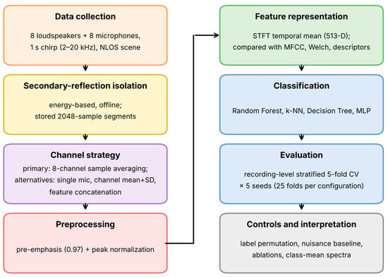
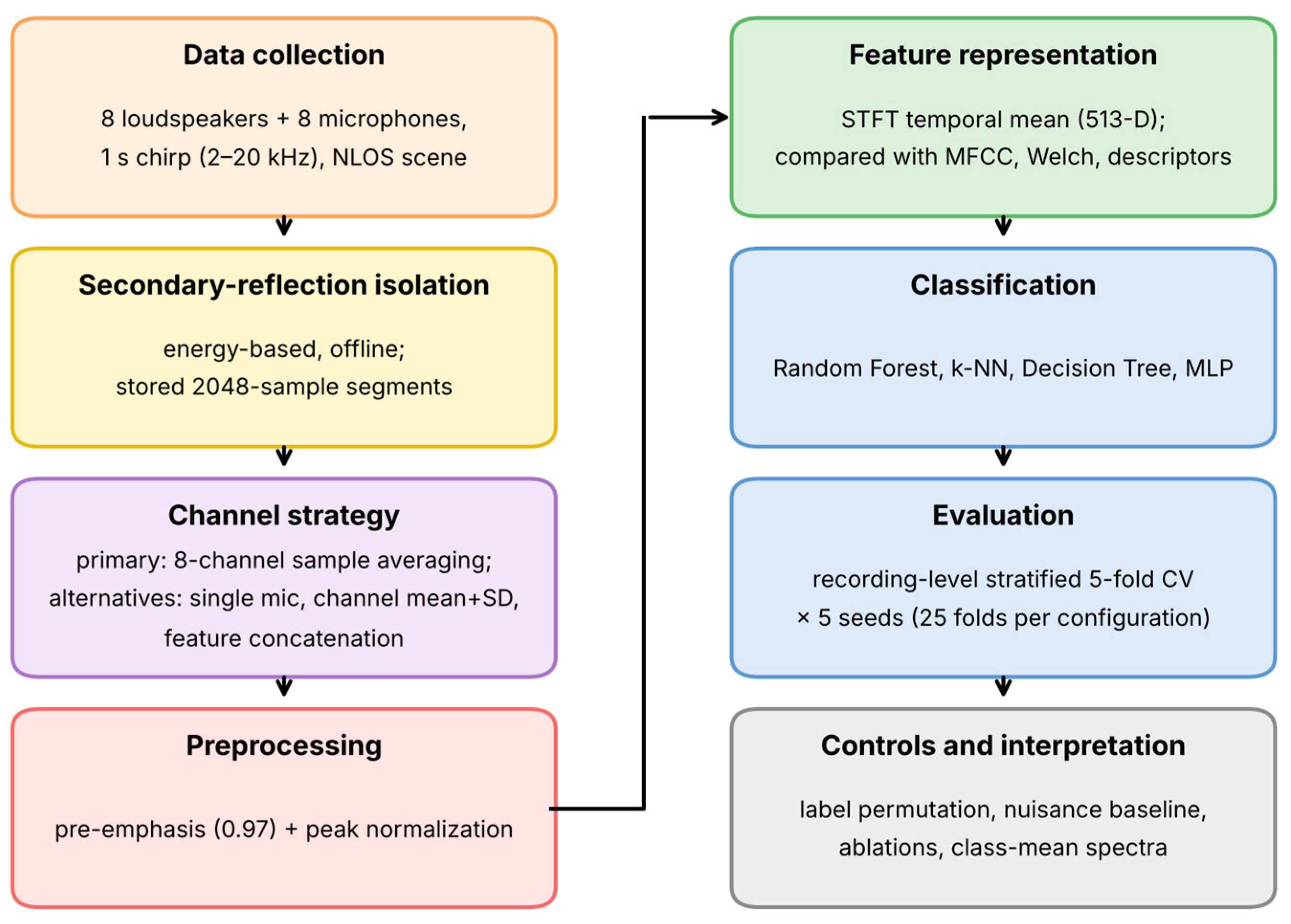
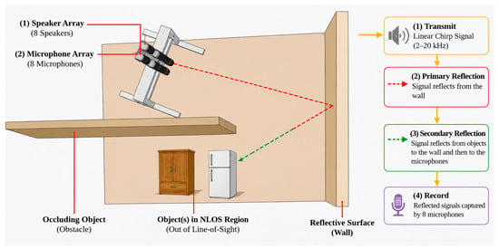
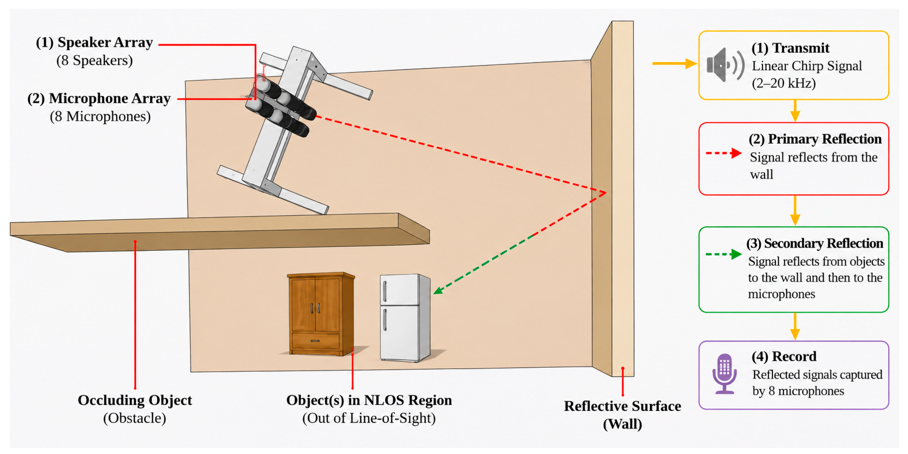
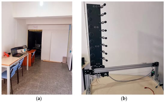
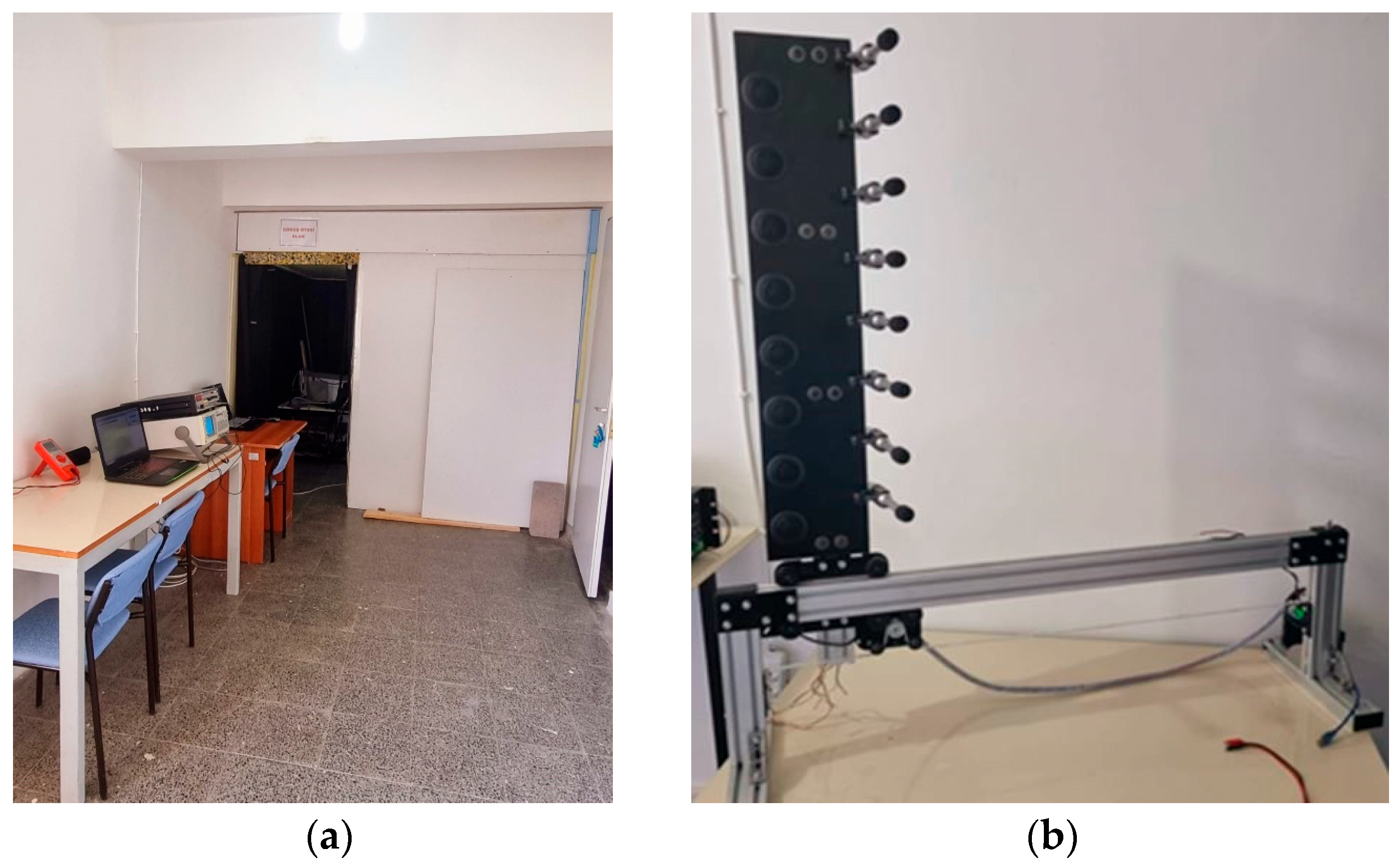
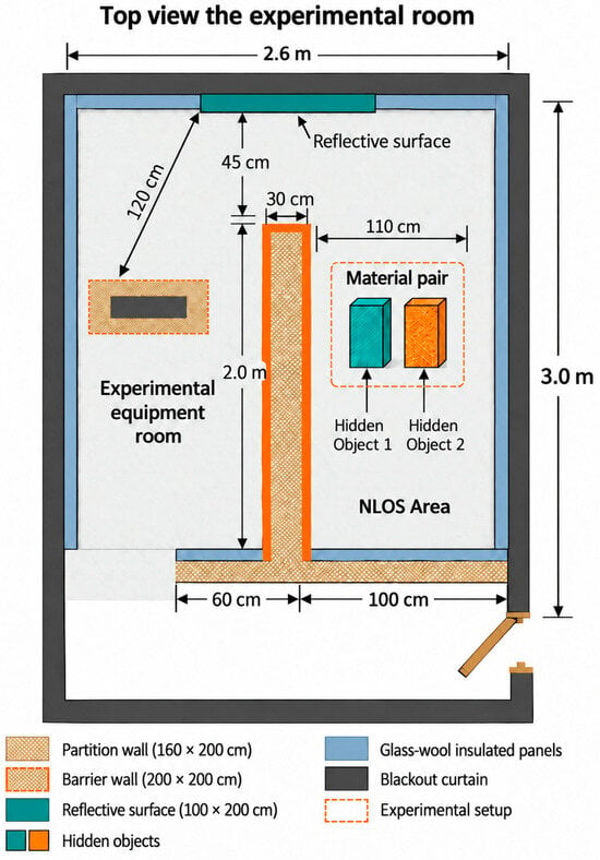
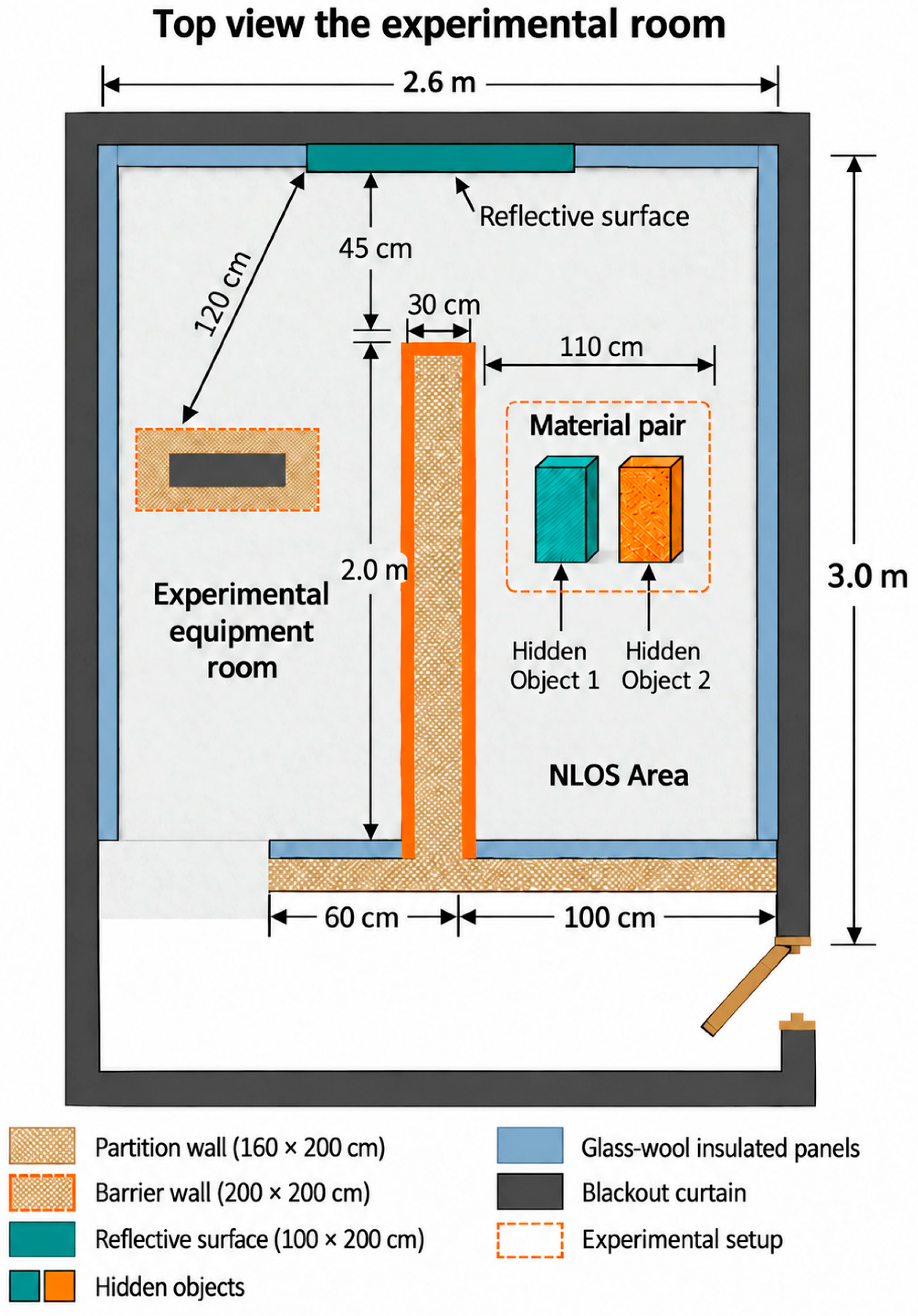
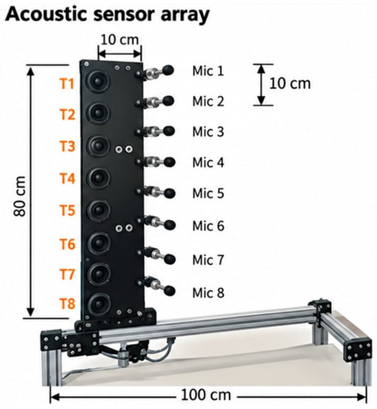
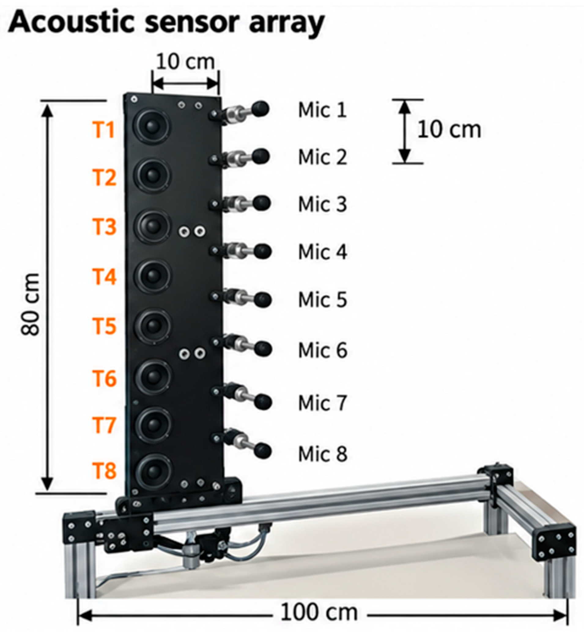
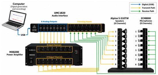
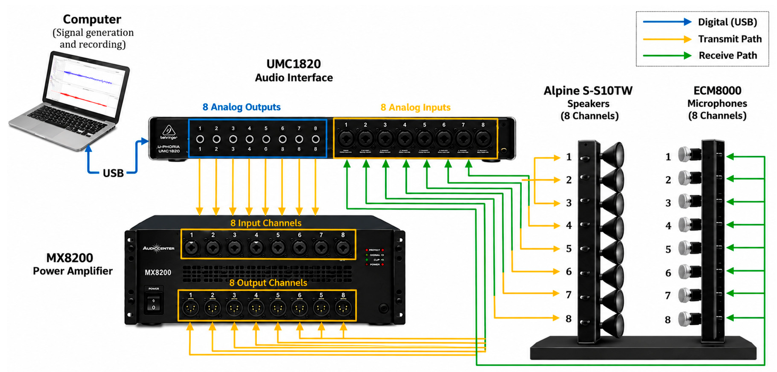
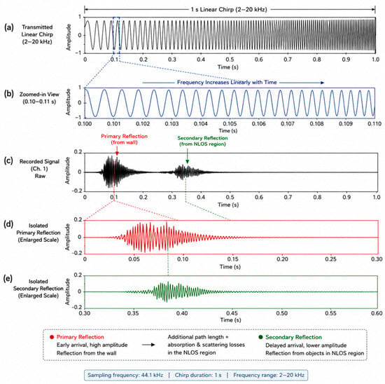
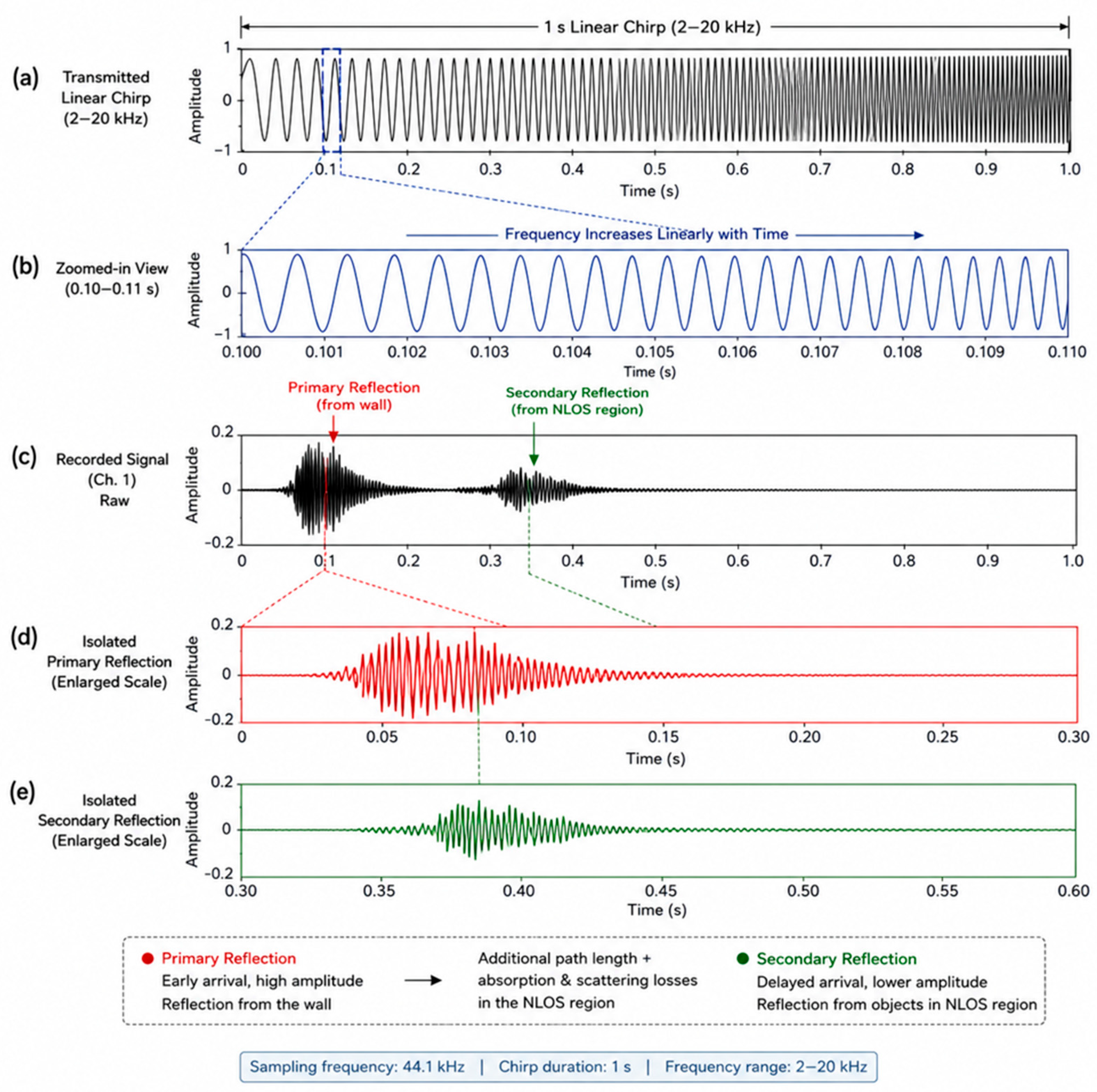
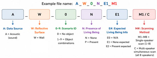
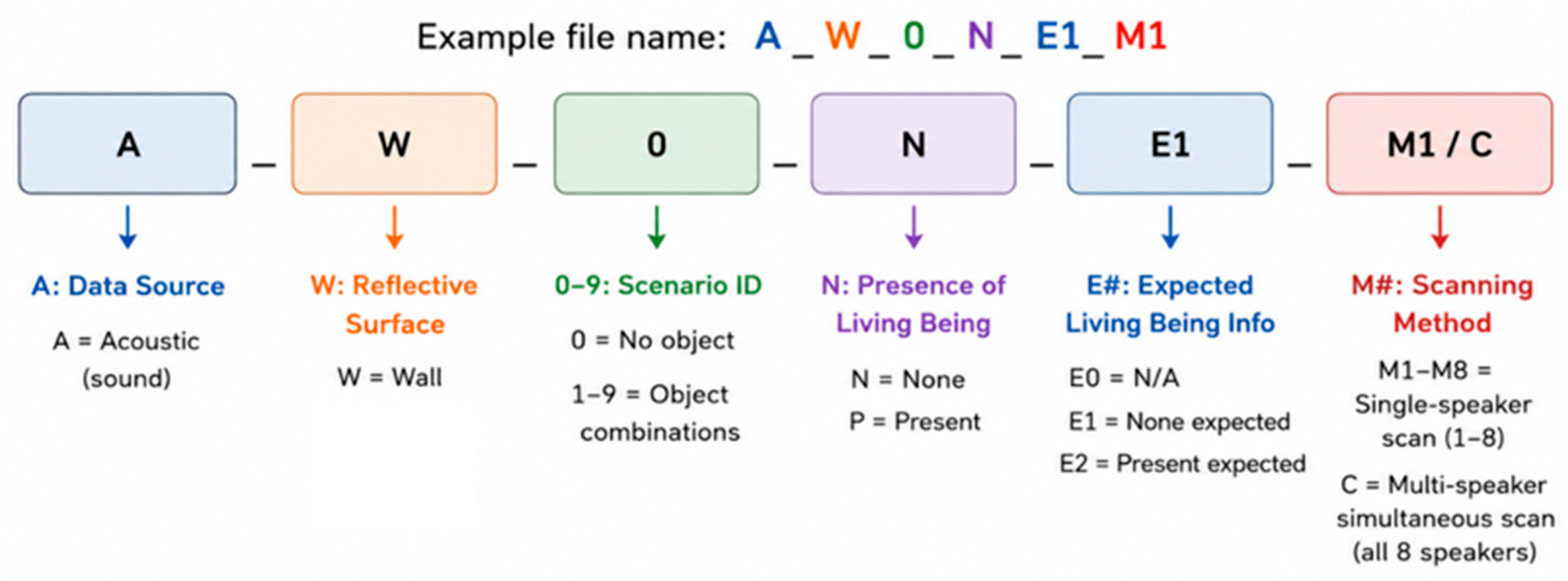
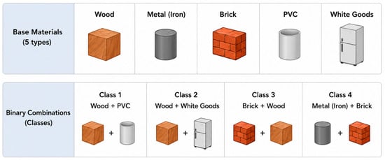
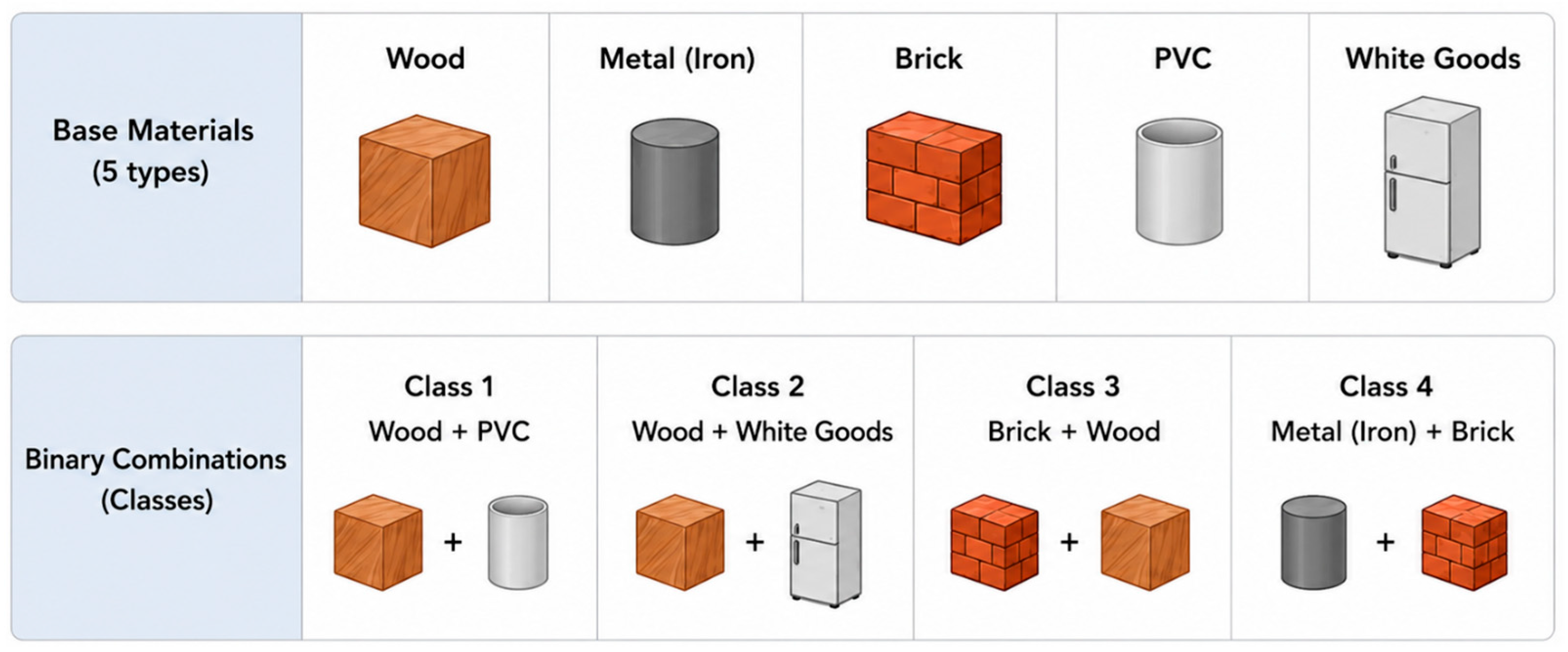
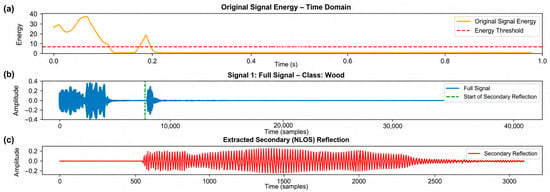
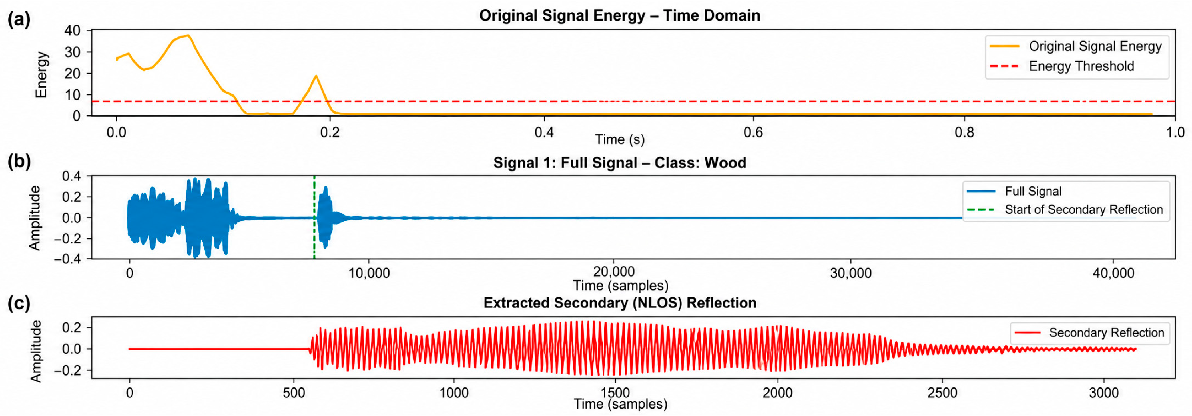
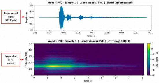
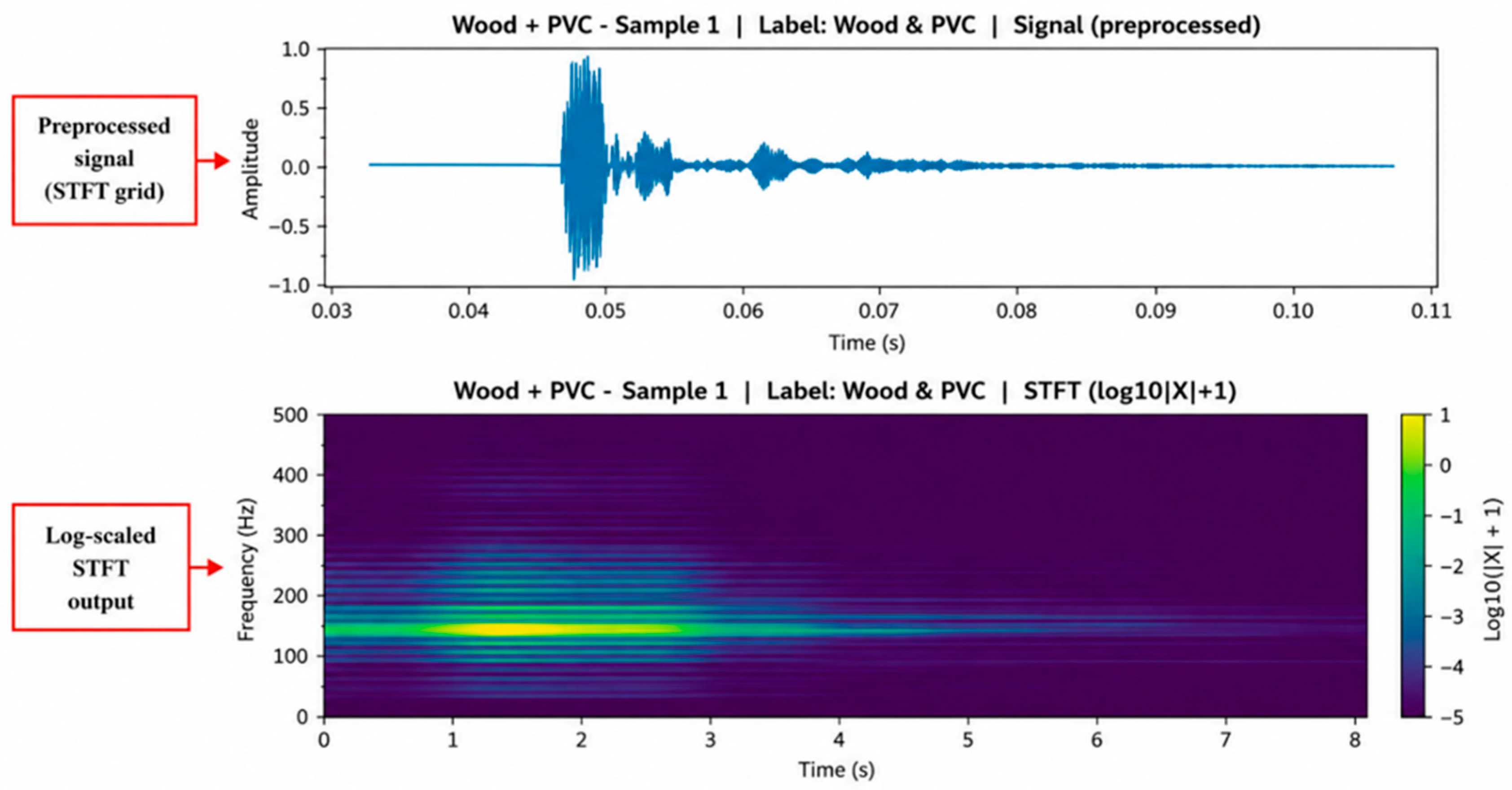
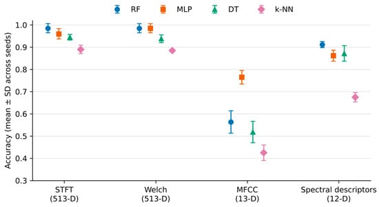
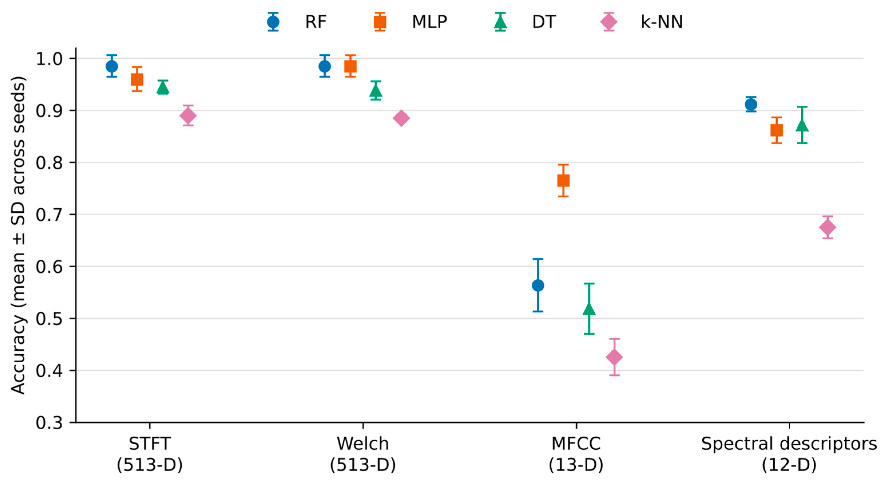
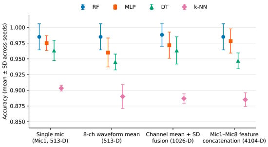
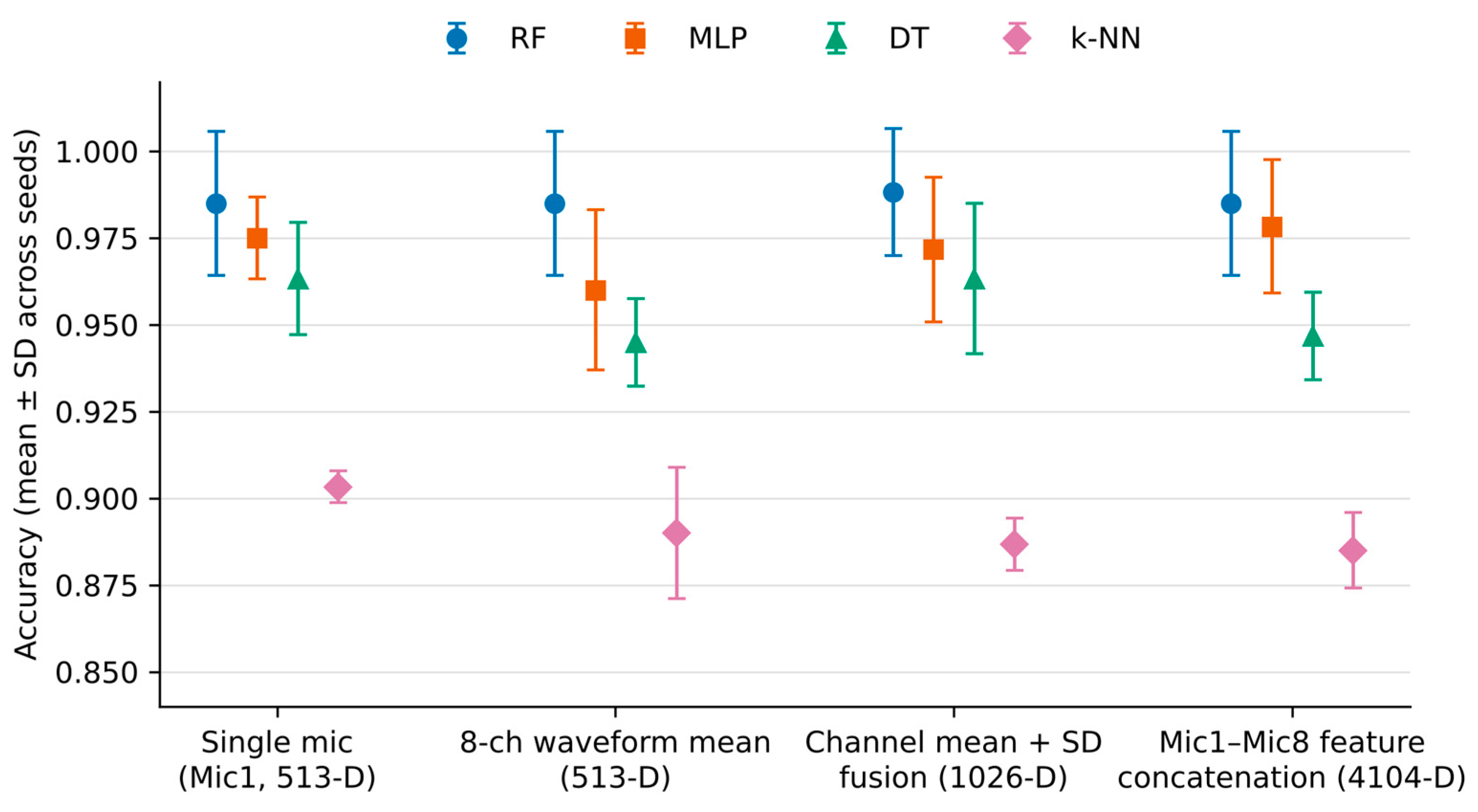
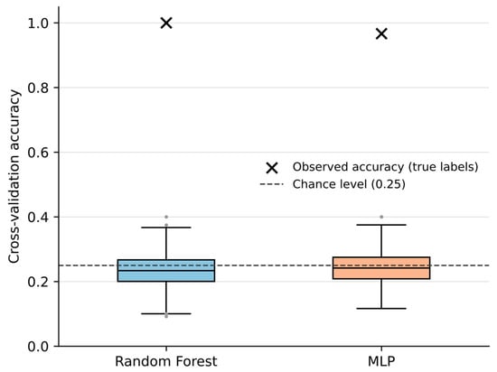
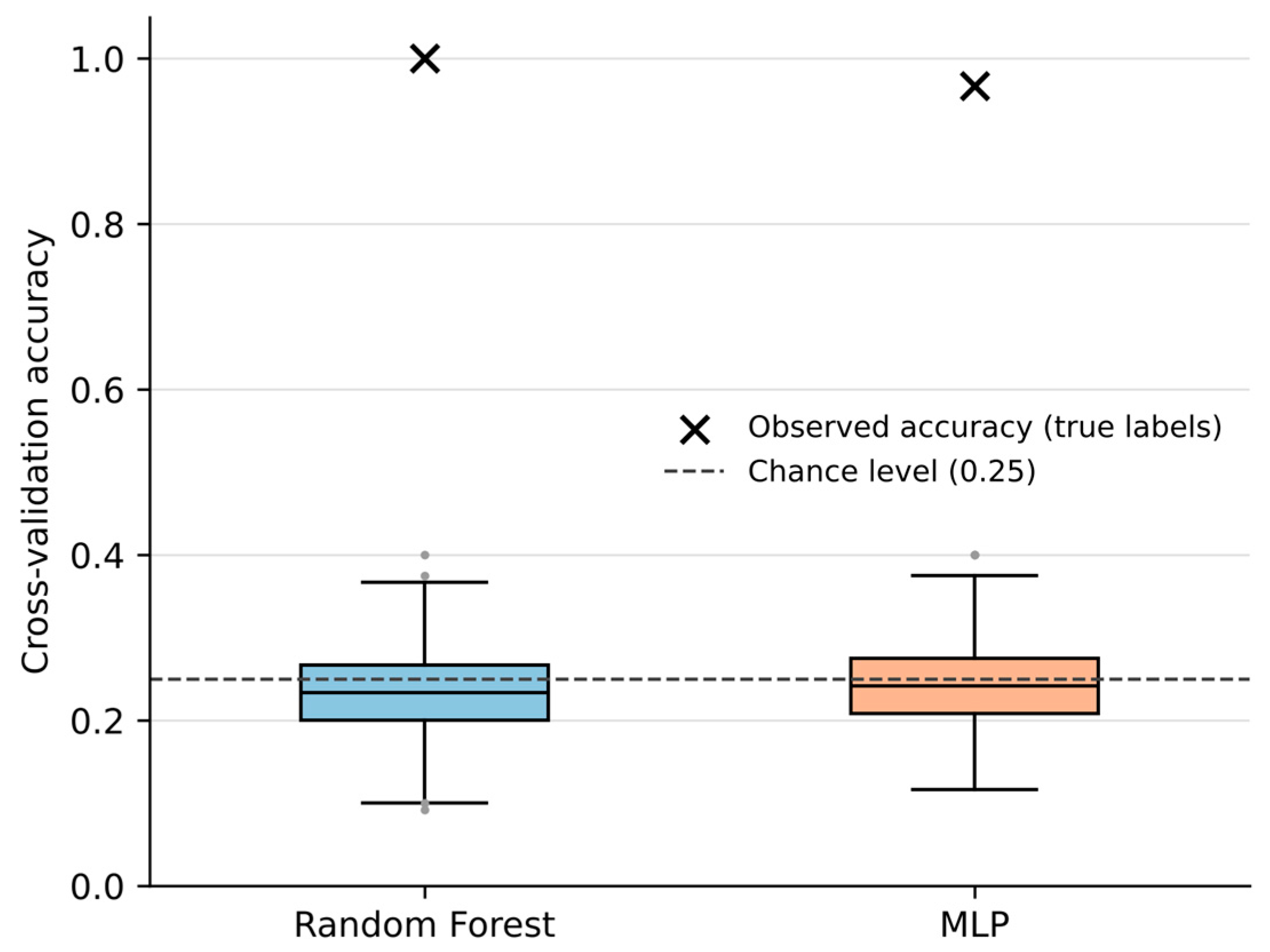
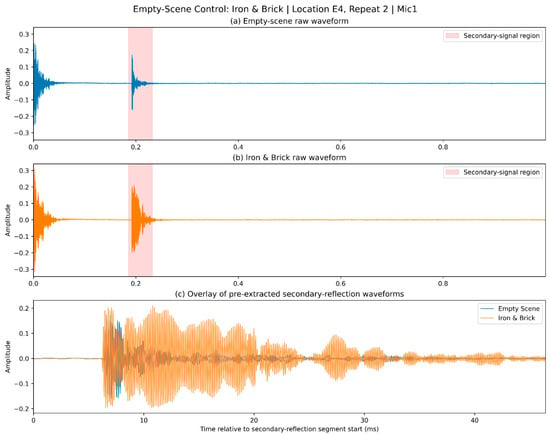
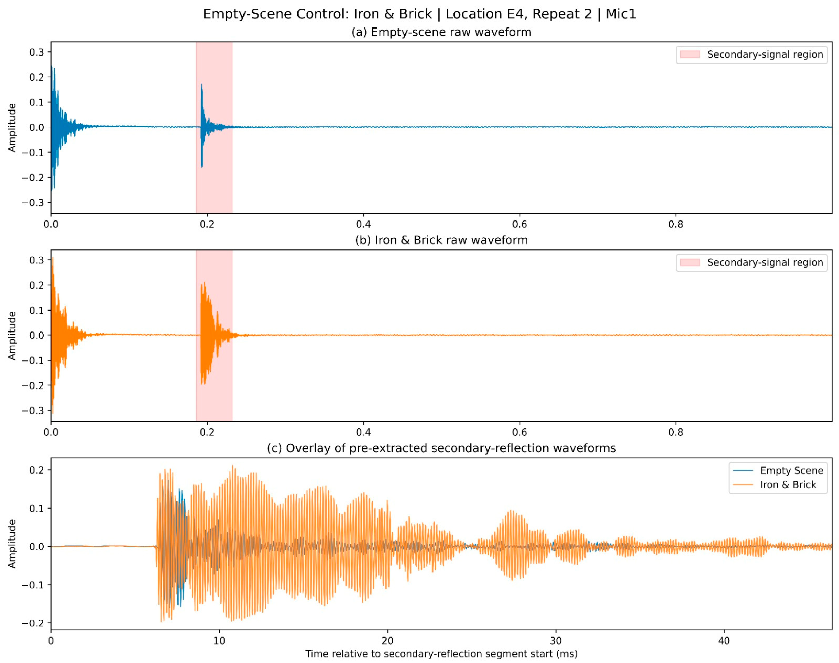
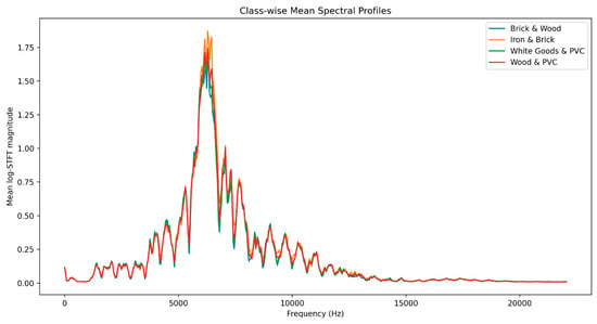
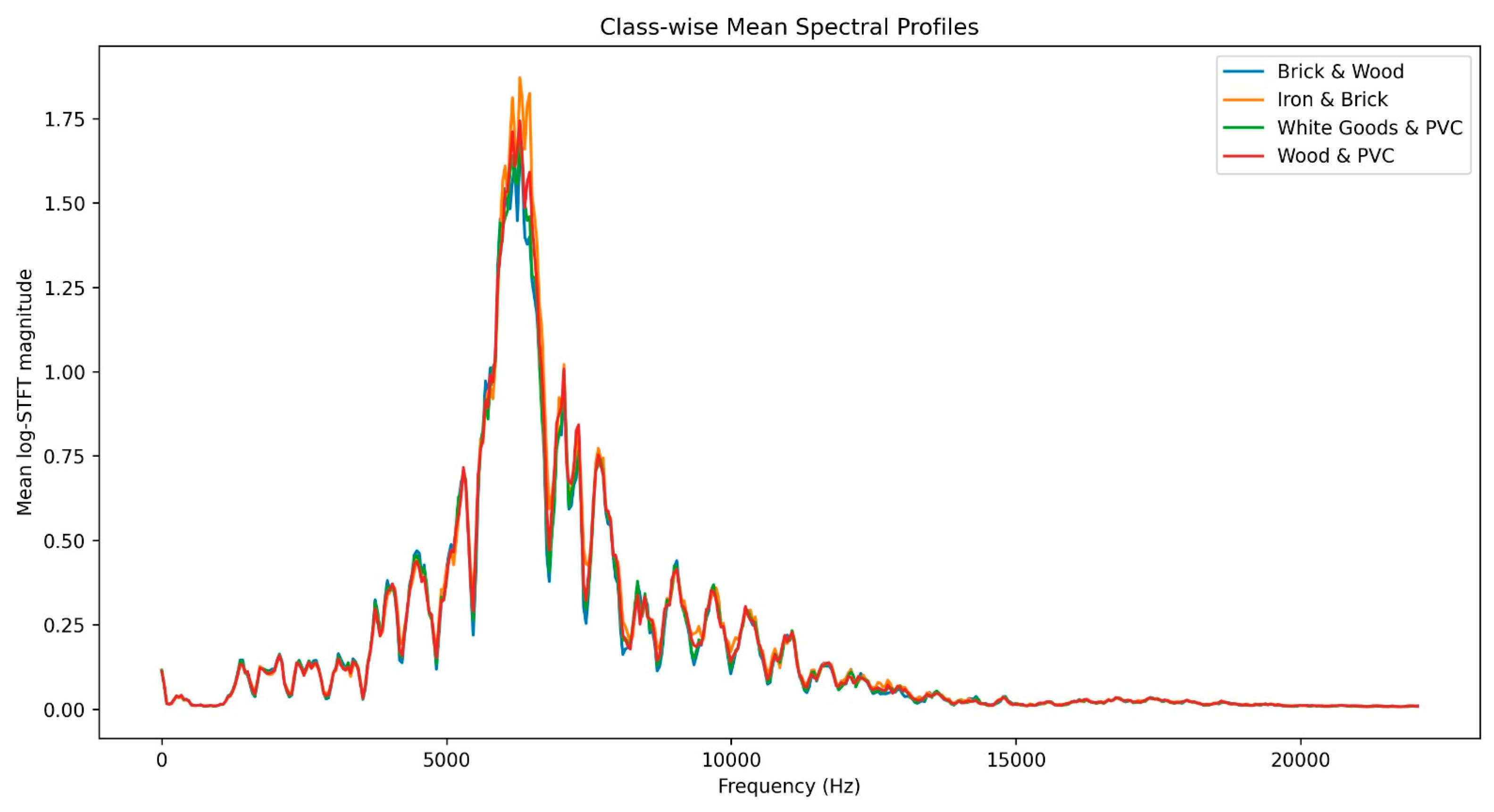

Disclaimer/Publisher’s Note: The statements, opinions and data contained in all publications are solely those of the individual author(s) and contributor(s) and not of MDPI and/or the editor(s). MDPI and/or the editor(s) disclaim responsibility for any injury to people or property resulting from any ideas, methods, instructions or products referred to in the content. |
© 2026 by the author. Licensee MDPI, Basel, Switzerland. This article is an open access article distributed under the terms and conditions of the Creative Commons Attribution (CC BY) license.