


Featured Application
The proposed method can be deployed in the structural health monitoring systems of long-span bridges to automatically identify vortex-induced vibration events from long-term acceleration records, thereby supporting routine vibration state assessment, fatigue accounting, and early warning of vortex-induced vibration risks without manual inspection of massive monitoring datasets.
Abstract
Vortex-induced vibration (VIV) occurs frequently on long-span bridges at low wind speeds and may cause fatigue damage and serviceability problems, so its reliable identification from field monitoring data is an important engineering task. However, existing automated identification methods rely mainly on single-point vibration indicators, and recognizing VIV events in massive, unlabeled monitoring datasets remains challenging. This study proposes an unsupervised VIV identification method based on a newly proposed feature, the Two-Point Vibration Phase Difference (TPVPD), computed between the vertical accelerations measured at the 1/4- and 3/4-span of the bridge. Because a VIV lock-in response is dominated by a single vibration mode, the phase difference between two spanwise locations remains nearly constant in time, whereas it fluctuates strongly under buffeting. The method was validated using six years (2013–2018) of monitoring data from a 1650-m main-span suspension bridge, covering 2.85 × 10⁵ valid 10-min windows. Spectral clustering of three features—acceleration RMS, TPVPD standard deviation, and an energy concentration coefficient—separated VIV from non-VIV states with a window-level F1 score of 0.84 with respect to a reference VIV inventory, and 99.8% of the windows identified as VIV exhibited spectral peaks at one of the six known VIV mode frequencies of the bridge. A rule-based cluster assignment calibrated on previous years transferred to subsequent years with F1 scores of 0.74–0.88, indicating the feasibility of operational deployment.
1. Introduction
As a typical form of wind-induced vibration, vortex-induced vibration (VIV) has been widely observed on long-span bridges worldwide [1,2]. Unlike flutter, which can cause divergent oscillations and structural failure, VIV generally does not lead to catastrophic collapse due to its amplitude-limited nature. However, as an aeroelastic resonance phenomenon, VIV can be triggered at relatively low wind speeds and occur frequently, leading to fatigue damage of bridge structures and affecting driving safety and comfort.
For instance, in 2012, the Volga River Bridge in Russia experienced pronounced vertical vibrations under wind speeds of 12–15 m/s [3]; the Trans-Tokyo Bay Crossing Bridge in Japan exhibited VIV with amplitudes up to 50 cm after its completion in 1993 [4]; on 5 May 2020, the Humen Bridge in Guangzhou, China, experienced its first VIV event in 23 years of service due to aerodynamic shape alterations caused by temporary facilities, with an amplitude of approximately 0.3 m [5]; and the Xihoumen Bridge, completed in 2009, has exhibited dozens of VIV events in recent years [6], posing a significant threat to operational safety.
Traditionally, studies in bridge aerodynamics have relied on three primary approaches: theoretical analysis, wind tunnel testing, and numerical simulation. These methods have yielded substantial insights into the aerodynamic forces acting on bridges. In wind tunnel studies, Kwok et al. [7] measured wind-induced pressures around sectional twin-deck bridge models and clarified the effects of gap width on the aerodynamic forces and vortex-shedding mechanisms; Trein et al. [8] examined the effects of the gap on the unsteady pressure characteristics of two-box bridge girders; Lee et al. [9] investigated the Reynolds-number sensitivity of the aerodynamic forces of a twin-box bridge girder; Ma et al. [10] experimentally studied the VIV of a twin-box girder with large cantilever plates; and Diana et al. [11] measured and modeled the vortex-shedding forces acting on a suspension bridge deck. Fundamental wind tunnel studies on rectangular prisms have further clarified how the aspect ratio governs the unsteady flow structures and the associated VIV response [12,13]. Based on these tests, various semi-empirical and theoretical models as well as corresponding parameter identification methods have been established. With the rapid development of computational fluid dynamics (CFD), significant progress has been made in simulating VIV numerically. Nevertheless, many CFD-based models still require parameters derived from wind tunnel experiments. Overall, both semi-empirical and CFD models depend heavily on accurate wind tunnel results. However, considerable discrepancies exist between wind tunnel conditions and actual field environments, such as high turbulence intensity, temporal variability, non-uniformity, and high Reynolds number effects. In addition, simplified models often fail to represent the detailed aerodynamic geometry of real bridges, including auxiliary structures, while VIV is highly sensitive to such subtle aerodynamic variations. These limitations make it challenging for traditional approaches to accurately simulate the complex VIV phenomena in full-scale long-span bridges.
With the advancement of modern sensing and structural health monitoring (SHM) technologies, field measurements have become increasingly crucial for studying wind-induced vibrations of bridges. Larsen et al. [14] observed VIV during the final stage of the Great Belt East Bridge construction and mitigated it effectively by installing guide vanes. Frandsen [15] further conducted simultaneous measurements of wind pressure and acceleration on the same bridge and found that under steady wind conditions with a mean velocity of approximately 8 m/s and flow direction nearly perpendicular to the bridge axis, lateral VIV occurred and the spatial correlation of wind pressure along the bridge span increased significantly. Dan et al. [6] analyzed multi-year monitoring data of the Xihoumen Bridge, identified dozens of VIV events, and developed a Gaussian process regression model for VIV prediction.
Beyond wind-induced vibration studies, bridge structural health monitoring (SHM) systems have been widely deployed to track structural conditions under operational and environmental actions, employing sensing technologies ranging from fiber-optic and vision-based devices to vibration-based monitoring networks [16,17]. The long-term monitoring data accumulated by these systems provide a valuable basis for data-driven identification of wind-induced vibration events, which motivates the automated identification approaches reviewed below.
However, field monitoring systems typically generate massive datasets, making manual identification of VIV events highly inefficient. In recent years, with the rapid progress of machine learning techniques, researchers have proposed numerous automated identification approaches. Li et al. [18] first employed a clustering-based method to distinguish VIV events from ordinary vibrations, using conventional root-mean-square (RMS) acceleration and an innovative Energy Concentration Coefficient (ECC)—defined as the ratio of the second to the first spectral peak—to characterize single-frequency vibration features, successfully achieving automatic VIV detection. Building on this, Xu et al. [19] integrated four features—mean wind speed, mean wind direction, acceleration RMS, and ECC—and developed a rule-based algorithm for comprehensive VIV identification. Huang et al. [20] proposed a random-decrement-based method for automatic identification of VIV events from long-term monitoring data. He et al. [21] introduced the Similarity Ratio of Amplitude feature derived from the complex domain representation of vibration signals, which quantifies the narrow-band circularity of Hilbert-transformed signals. Combined with the ECC, their method also achieved effective VIV recognition and could further distinguish formation, steady, and decay stages of vibration.
In practical applications, bridge monitoring datasets often contain limited or no VIV samples, making it essential to develop algorithms that can operate under data-scarce conditions. Hou et al. [22] proposed a transfer learning approach based on Transfer Component Analysis, which projects data from different bridges into a unified feature space and employs a support vector machine (SVM) for classification. Their results demonstrated that the method outperformed baseline SVM models even without historical VIV data. Kim et al. [23] developed recognition strategies for both zero-sample and few-sample scenarios using probabilistic regression, neural networks, autoencoders, and deep clustering, achieving robust discrimination between VIV and non-VIV events under various monitoring conditions. Lim et al. [24] proposed a semi-supervised three-step algorithm that requires no manual labeling. Using RMS acceleration, energy ratio factor, first five spectral amplitudes, peak factor, mean wind speed, and wind direction as input features, their method (1) automatically labels a small subset of data based on the peak factor, (2) expands labels using a binary deep neural network, and (3) determines the optimal threshold for the peak factor based on the network’s output. Validation using both short-term and long-term field data of long-span bridges demonstrated high classification accuracy.
In summary, existing studies have made significant advances in feature extraction and automated recognition of VIV events. However, most current methods rely on single-point vibration measurements. This paper proposes a new field-based VIV identification feature—the phase-difference feature calculated between acceleration signals at two different locations along the bridge—TPVPD. This feature is highly sensitive to structural synchronization changes and provides high temporal resolution. Based on this feature, a machine-learning-based approach is further developed for automatic identification of vortex-induced vibration events in long-span bridges.
2. Methods
2.1. Two-Point Vibration Phase Difference Feature
The main girder of the bridge is treated as an N-degree-of-freedom forced vibration system. Considering this, the dynamic equation of the N-degree-of-freedom vibration system is expressed as
Expressed using the state vector,
Substituting Equation (2) into Equation (1),
where .
When a bridge undergoes vortex-induced vibration, the lock-in response is dominated by a single structural mode and exhibits obvious single-frequency characteristics. This single-mode dominance is the key property on which the following derivation relies. Note that the formulation below is written for the free decay of a single mode for clarity of notation; the same phase property holds for the steady single-mode forced or self-excited response excited by vortex shedding, because the response can then be approximated as a narrow-band process dominated by that mode. Assuming that the dominant response occurs in the s-th mode of the bridge, we have
In the formula, denotes the s-th order mode shape vector, and q represents the complex modal generalized coordinate, which can be expanded as
Thus,
Substituting Equation (4) into Equation (2) gives
Substituting the above equation into the formula (3) and considering the case of free vibration, we obtain
Multiply both sides of the equation by on the left simultaneously, yielding
where , and both a and b are constants.
The solution to this equation is
Let the s-th order mode be expanded as
Then the displacement of the i-th degree of freedom of the structure can be expressed as
To express the complex number in the above equation in the form of modulus and phase angle, we set
where and denote the modal coefficient and the amplitude of the modal coordinate at the i-th point of the r-th order mode, respectively; and represent their phase angles, respectively; and stand for the real part and the imaginary part of the complex modal frequency, respectively. Substitute them into the formula (12) and sort out the results to obtain
Then the unique response vector of each point on the bridge deck is
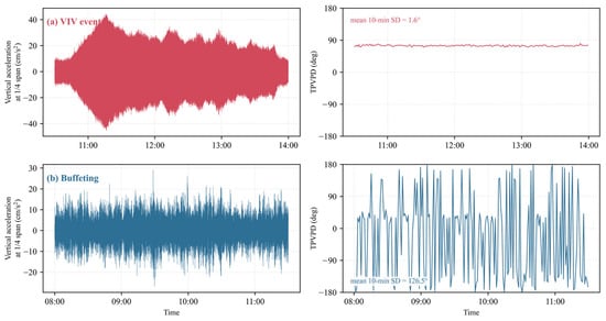
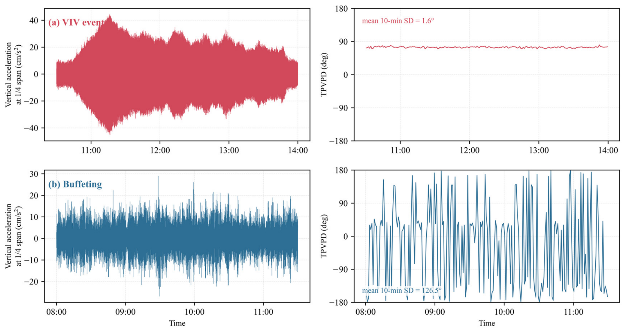
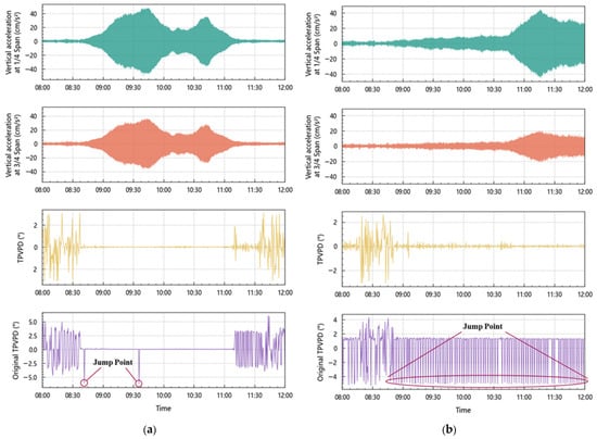
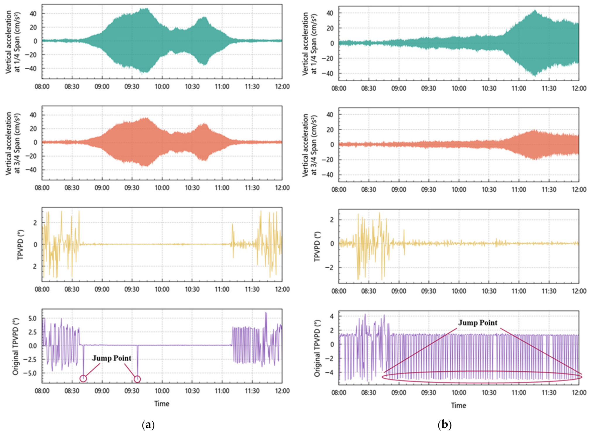
It is noted that γsi is time-independent and varies among different points; therefore, for a single-mode-dominated response, there is a time-invariant phase difference between different points of the structure. For instance, in an actual bridge structure, a stable phase difference that remains unchanged with time exists between two different points (denoted as m and n) along the spanwise direction of the bridge. Two clarifications are required here. First, although the derivation is formulated in terms of displacement, it applies directly to acceleration: for a single-mode harmonic response, the acceleration differs from the displacement only by a constant factor −ωs2 and a constant phase shift of π, so the phase difference between two measurement points is identical for the two quantities. Second, the time-invariant inter-point phase difference is a characteristic of single-mode-dominated responses rather than an exclusive signature of VIV; in principle, any sufficiently narrow-band response dominated by one mode would exhibit a similar property. During VIV, however, lock-in produces a persistent, high-amplitude single-mode response, so a stably synchronized phase difference emerges naturally and robustly. By contrast, under buffeting the response is distributed over many modes, and the inter-point phase difference exhibits significant temporal fluctuations and lacks stable synchronization. Figure 1 presents this contrast for a representative case: the 10-min standard deviation of TPVPD averages 1.6° during a VIV event, against 126.5° during a strong buffeting episode. Consequently, TPVPD should be regarded as a useful feature for identifying single-mode-dominated responses rather than a unique physical signature of VIV, and it is therefore used in combination with amplitude and spectral indicators (Section 3.3 and Section 3.4) to distinguish VIV from other responses; the possible confounding responses are further discussed in Section 4.
Figure 1.
Comparison of TPVPD between a VIV event and a strong buffeting episode: (a) VIV event (0.327 Hz mode, 14 October 2014), with a mean 10-min TPVPD standard deviation of 1.6°; (b) buffeting episode (24 January 2016, mean wind speed up to 24.6 m/s), with a mean 10-min TPVPD standard deviation of 126.5°.
2.2. Spectral Clustering Method
Spectral clustering is a graph-based unsupervised learning method that has been widely applied in complex pattern recognition problems due to its strong capability in handling nonlinearly separable data distributions. Unlike traditional centroid-based clustering algorithms such as k-means, spectral clustering performs clustering in a transformed feature space derived from the spectral properties of a similarity graph, which makes it particularly suitable for vibration response data exhibiting nonlinear relationships and irregular cluster shapes.
Given a dataset
where each sample represents a feature vector extracted from bridge monitoring data (e.g., acceleration RMS and TPVPD statistics), spectral clustering first constructs an undirected similarity graph G = (V, E). Each node corresponds to a data sample, and the edge weight between nodes i and j is defined by a similarity function. A common choice is the Gaussian kernel:
where σ is the scaling parameter controlling the sensitivity of similarity decay. The fully connected Gaussian-kernel graph is, however, sensitive to the choice of σ and becomes computationally expensive for large datasets. In this study, a symmetric k-nearest-neighbor (kNN) graph is therefore adopted instead of Equation (19): Wij = 1 if node j is among the k nearest neighbors of node i or vice versa, and Wij = 0 otherwise, with k = 10. This construction is robust to local density variations, avoids the manual specification of σ, and scales efficiently to the annual datasets considered here (4.5 × 10⁴–4.9 × 10⁴ samples per year). The degree matrix and the normalized Laplacian below are formed from this W.
Based on the similarity matrix , the degree matrix D is defined as
and the normalized graph Laplacian is constructed as
Spectral clustering then solves the eigenvalue problem of Lsym and selects the first K eigenvectors corresponding to the smallest eigenvalues to form a low-dimensional embedding matrix U ∈ RN×K, computed with the ARPACK implicitly restarted Lanczos method. Each row of U represents a transformed feature vector capturing the intrinsic connectivity structure of the original dataset.
Finally, k-means (ten restarts, n_init = 10) is applied in the embedded space to partition the data into K clusters. Since the mapping is guided by the graph structure rather than Euclidean distances in the original space, spectral clustering can effectively separate vibration patterns with subtle differences but strong internal consistency. All analyses in this study were implemented in Python 3.10 using scikit-learn 1.6.1; for one annual dataset (≈4.8 × 10⁴ samples), z-score normalization, graph construction, eigendecomposition, and k-means assignment take less than one minute in total on a desktop CPU (Intel Core i7-12700).
In the context of vortex-induced vibration identification, VIV responses are characterized by relatively stable phase synchronization and distinct amplitude levels, which result in stronger intra-cluster similarity in the TPVPD-based feature space. Spectral clustering exploits this property by grouping samples according to their global similarity structure, enabling robust automatic identification of VIV events without relying on manually labeled data.
3. Identification of VIVs in the Long-Term Monitoring Dataset
3.1. Introduction to Bridge Health Monitoring System
Since wind tunnel tests cannot reproduce the high turbulence intensity, temporal variability, non-uniformity, and high Reynolds number effects of natural wind fields, the experimental results often differ significantly from the actual behavior of full-scale long-span bridges. Therefore, field monitoring data provide the most comprehensive and realistic representation of VIV phenomena in long-span bridges under natural wind excitation. In this study, a long-span bridge located in the field is taken as an example to illustrate the proposed VIV identification framework.
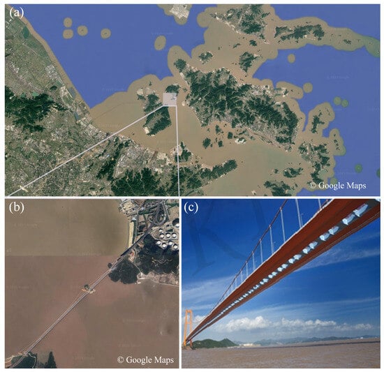
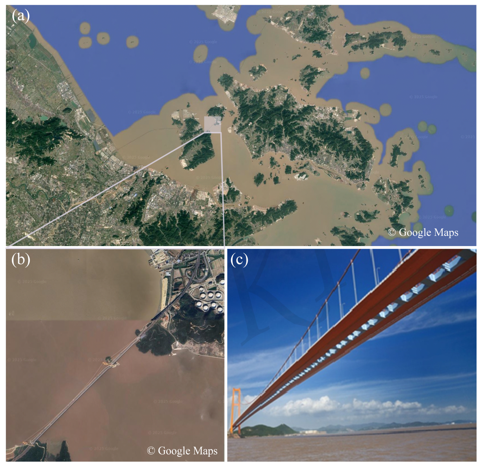
The bridge investigated in this paper is located in eastern China, connecting two islands, which is shown in Figure 2. It is a steel box girder suspension bridge with a main span of 1650 m. The region is characterized by strong and variable wind conditions due to its unique geographic environment—it is frequently affected not only by steady monsoon flows at low wind speeds but also by strong seasonal winds and typhoons. The bridge is equipped with a comprehensive SHM system, which includes anemometers for wind measurements and accelerometers for vibration monitoring of the main girder.
Figure 2.
Location of the investigated bridge: (a) geographic location; (b) satellite view of the bridge; (c) view of the main girder. Base maps: © 2025 Google; photograph: reproduced from the corresponding author’s PhD dissertation.
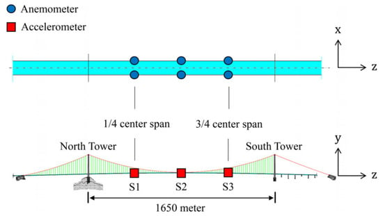
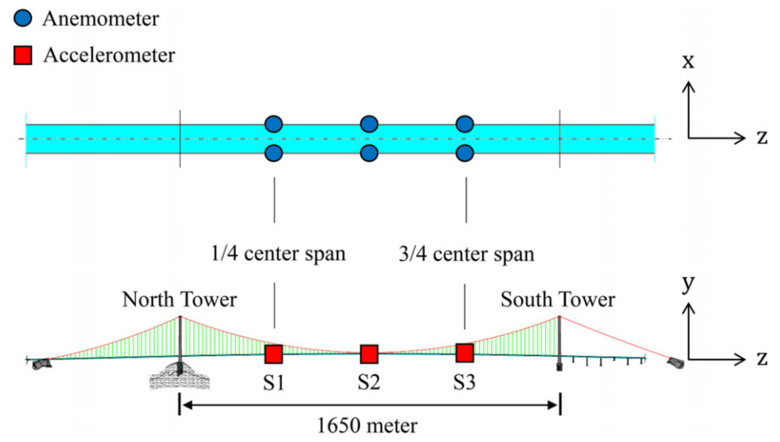
The sensors used for monitoring the wind environment and structural vibration are shown in Figure 3. Six Wind Master Pro three-dimensional ultrasonic anemometers are installed at the 1/4-span, mid-span, and 3/4-span positions (denoted as S1, S2, and S3), with one on each side of the bridge deck. All anemometers are mounted on 6-m-high lamp posts to minimize aerodynamic interference from the bridge structure. Each anemometer measures three-dimensional wind velocity within a range of 0–60 m/s at a sampling frequency of 32 Hz. The raw data consist of three orthogonal wind components (ux, uᵧ, and uz). To avoid the influence of wake effects from the bridge structure, only the upwind anemometer data corresponding to the current wind direction are used for analysis.
Figure 3.
Locations of anemometers and accelerometers.
Similarly, six accelerometers are installed at the same spanwise positions as the anemometers (i.e., on both sides of S1, S2, and S3) to record the lateral and vertical vibrations of the bridge deck, with a sampling frequency of 50 Hz. Since VIV typically manifests as crossflow oscillations, only the vertical acceleration data are considered in this study. At each spanwise position, the vertical accelerations recorded by the two accelerometers on the two sides of the deck were averaged to represent the vertical motion at the center of the deck cross-section; torsional effects are therefore not considered and are listed among the limitations in Section 4. All acceleration channels were recorded simultaneously by the same data acquisition system, so the inter-channel synchronization error is negligible for phase-difference calculation.
3.2. Data Analysis
In this study, six years of long-term monitoring data from 2013 to 2018 were utilized for model development and analysis.
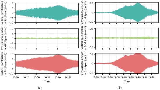
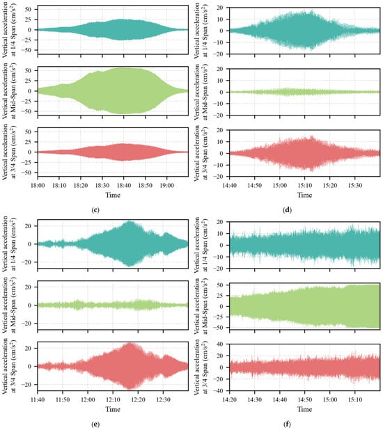
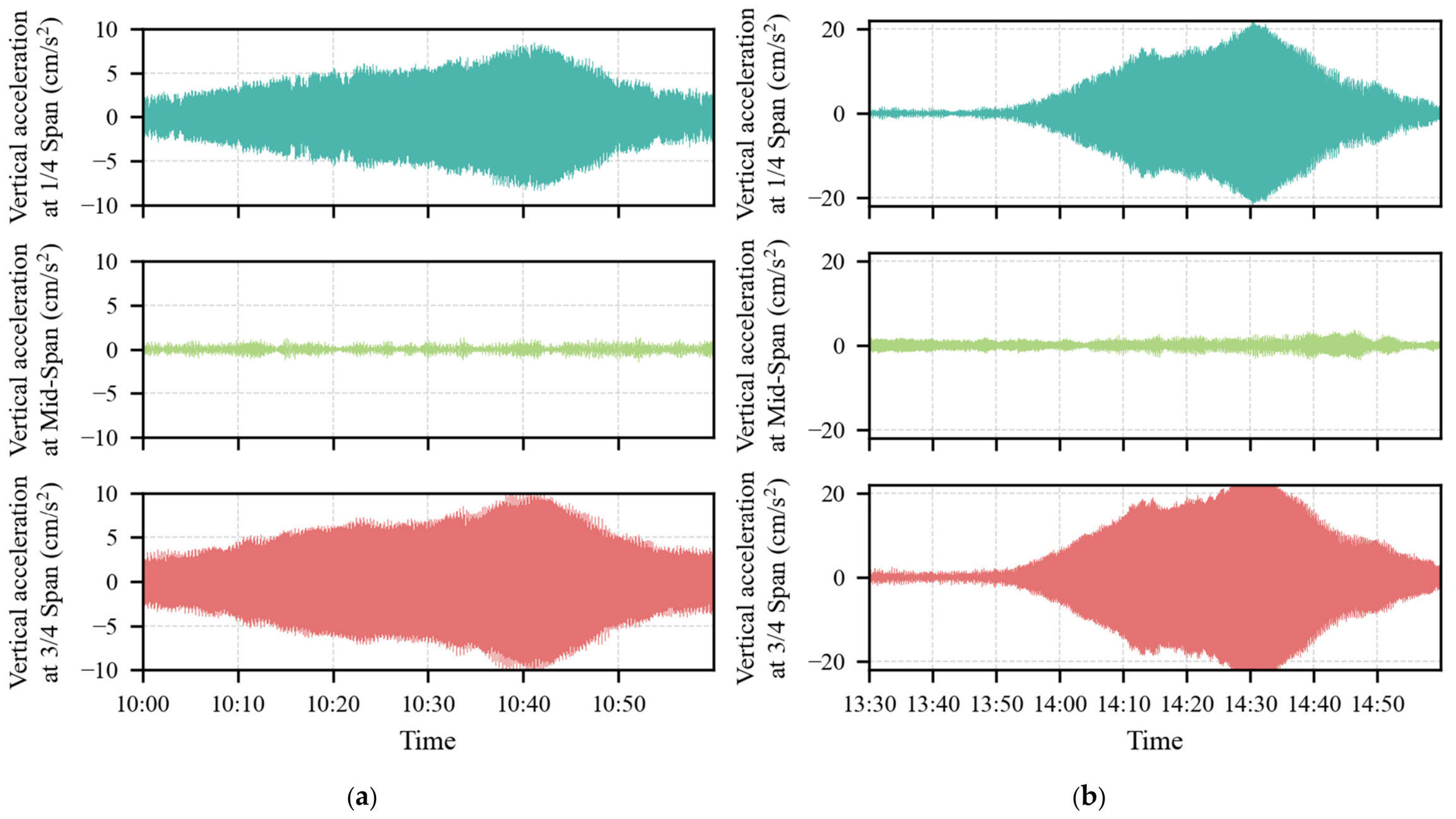
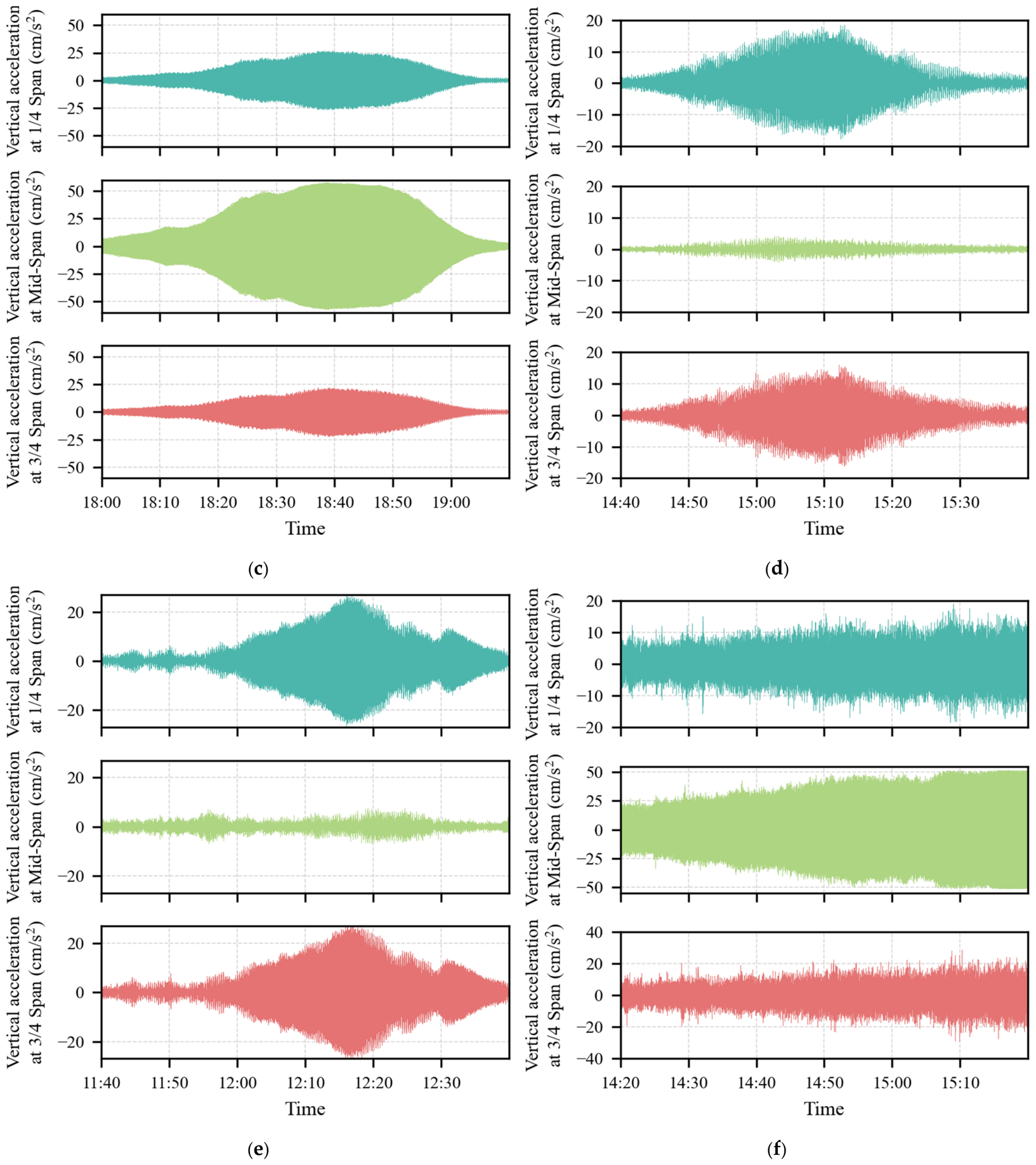
To date, six distinct VIV modes have been identified from the monitoring dataset of the bridge, with dominant frequencies of 0.183 Hz, 0.276 Hz, 0.327 Hz, 0.378 Hz, 0.435 Hz, and 0.495 Hz [18]. The characteristics of the six modes are summarized in Table 1. Analysis of the vibration records indicates that the nodal points of the 0.183, 0.276, 0.378, and 0.495 Hz modes are located near the mid-span, resulting in relatively small mid-span amplitudes during the corresponding VIV events, whereas the 0.327 Hz and 0.435 Hz modes exhibit a wave loop at mid-span and produce much larger mid-span responses (Figure 4).
Table 1.
Summary of the six identified VIV modes (window counts refer to windows classified as VIV in 2013–2018 whose spectral peak falls within ±0.01 Hz of the mode frequency).
Figure 4.
Vibration signals of each mode: (a) 0.183 Hz; (b) 0.276 Hz; (c) 0.327 Hz; (d) 0.378 Hz; (e) 0.495 Hz; (f) 0.435 Hz.
Accordingly, to capture the most representative vibration characteristics, subsequent analyses in this study focus on the acceleration data obtained from the 1/4-span and 3/4-span positions (denoted as S1 and S3). These locations correspond to the wave loop of the vibration modes, where the dynamic responses during VIV events are the most pronounced, providing a more sensitive and reliable basis for feature extraction and event identification. This choice remains valid for the 0.327 Hz and 0.435 Hz modes, because S1 and S3 are also located near wave loops for these modes (Table 1).
3.3. Two-Point Vibration Phase Difference (TPVPD)
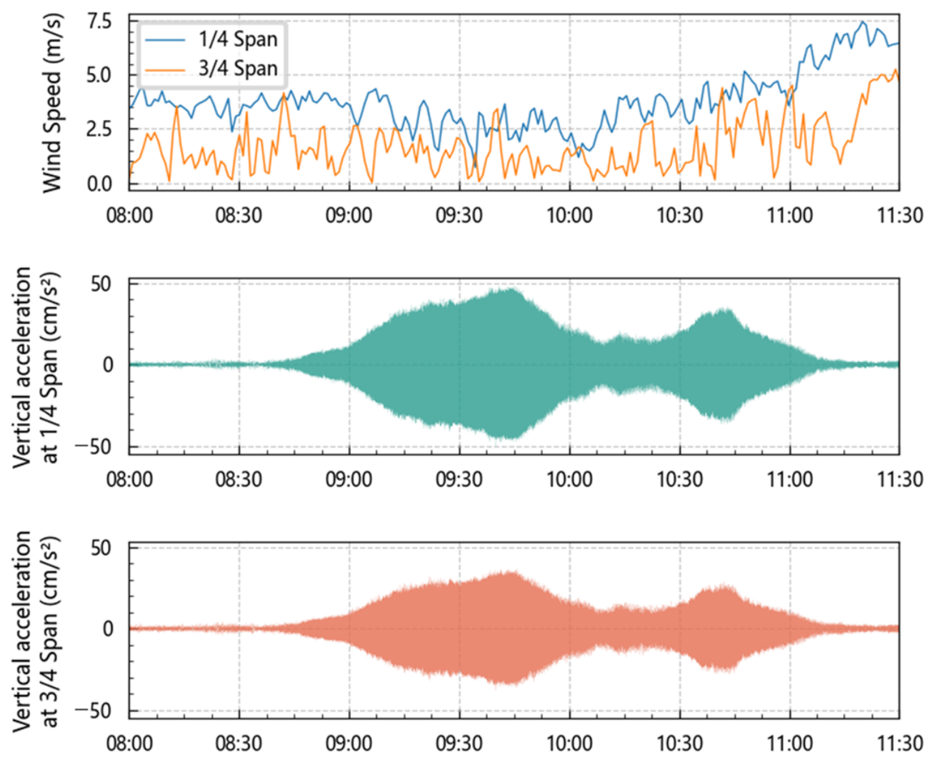
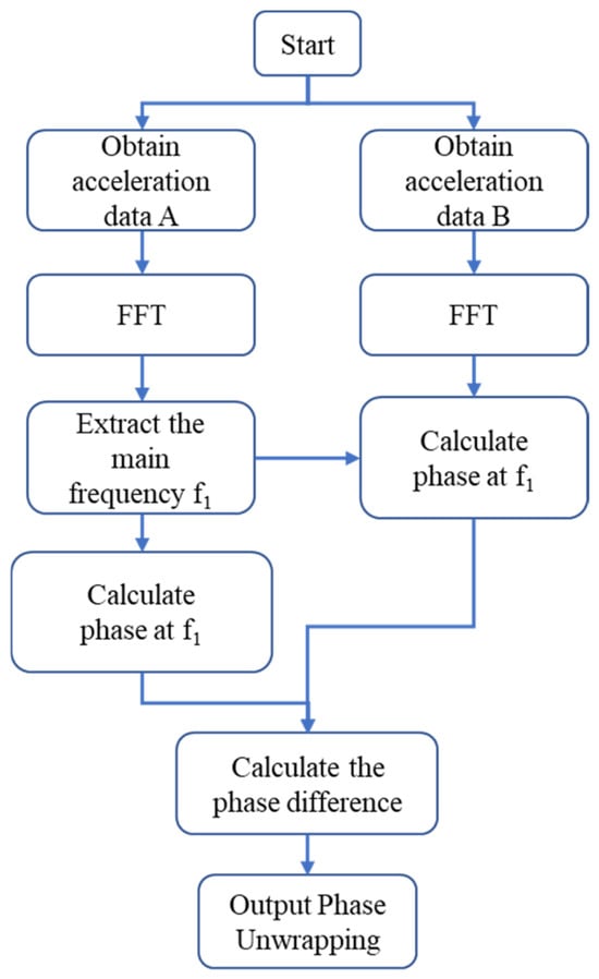
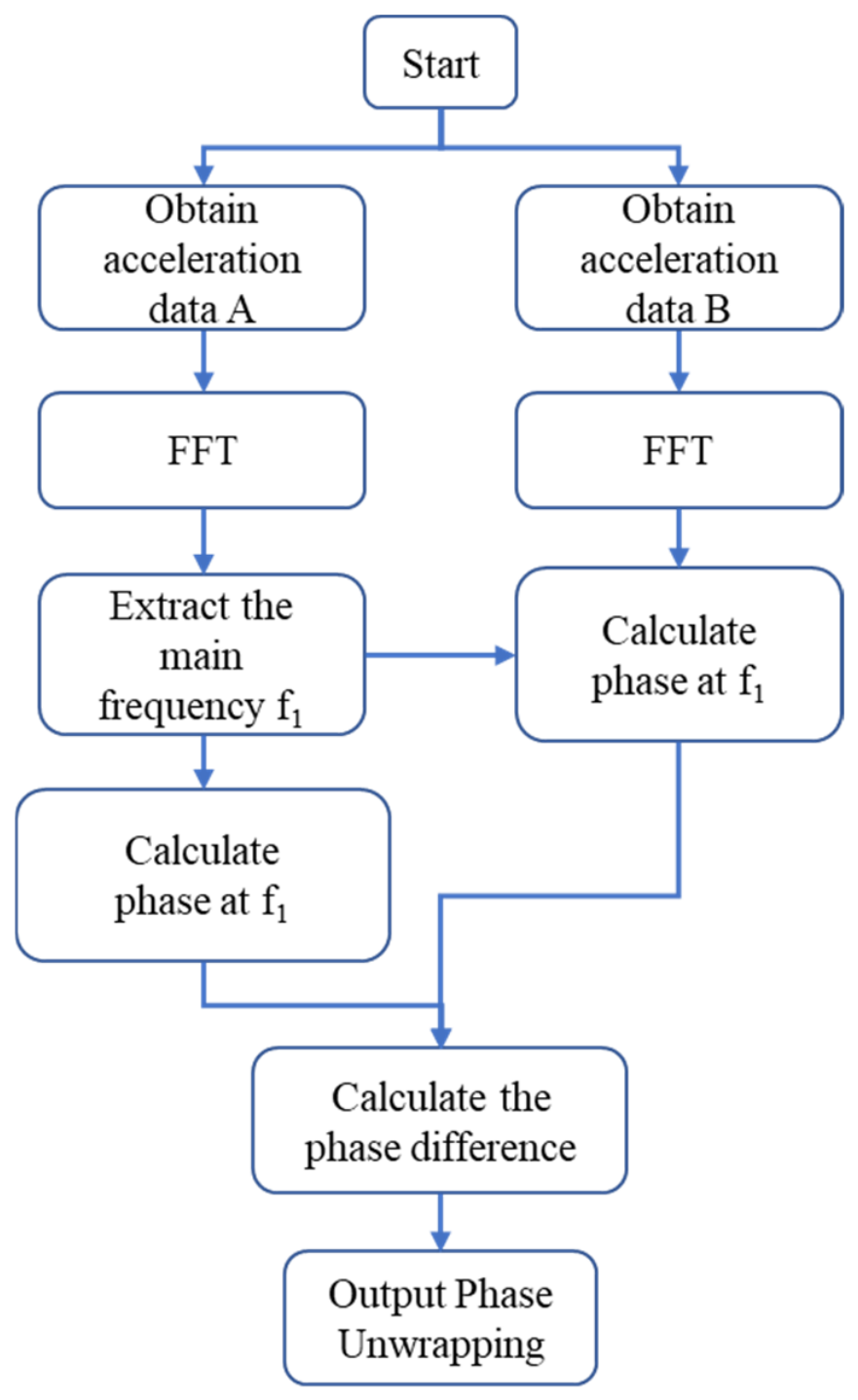
Figure 5 presents the variations in wind speed and vibration acceleration during a representative VIV event. As shown, the vibration amplitude increases progressively throughout the VIV process and returns to its normal level once the event subsides. Consequently, the RMS value of acceleration can be regarded as a key indicator for distinguishing VIV events from ordinary background vibrations. The overall computational framework for the analysis is illustrated in Figure 6.
Figure 5.
Wind speed and vibration acceleration during a typical VIV event.
Figure 6.
Overall framework of the proposed VIV identification method.
Based on the derivation presented in Section 2, the Two-Point Vibration Phase Difference (TPVPD) was computed using the vertical acceleration data obtained from positions S1 and S3. For each non-overlapping T-second segment, the dominant frequency is defined as the frequency at which the amplitude spectrum of the 1/4-span acceleration, obtained by a fast Fourier transform with a frequency resolution of 1/T, is maximal; the phase difference is the difference between the FFT phase angles of the two signals at this frequency bin, and no filtering or tapering is applied at this stage. In practical implementation, the calculated phase difference is confined within the range (−π, π]. As a result, discontinuities may appear when the phase difference approaches either boundary, as illustrated in Figure 7. To remove these abrupt phase jumps and maintain continuity, an unwrap operation was applied to the TPVPD sequence. Denoting the wrapped difference in the i-th segment by Pi, the unwrapped sequence is obtained from Equation (22):
where wrap(·) denotes the function that maps its argument into (−π, π] by adding an integer multiple of 2π, i.e., wrap(x) = x − 2π·round(x/2π). Segments containing missing samples are discarded, and the 10-min value of TPVPD is summarized by the standard deviation of the unwrapped sequence within the window. Because the unwrapped phase difference of a synchronized response varies slowly, circular statistics are not required.
Figure 7.
Comparison of TPVPD before and after unwrapping: (a) wrapped; (b) unwrapped.
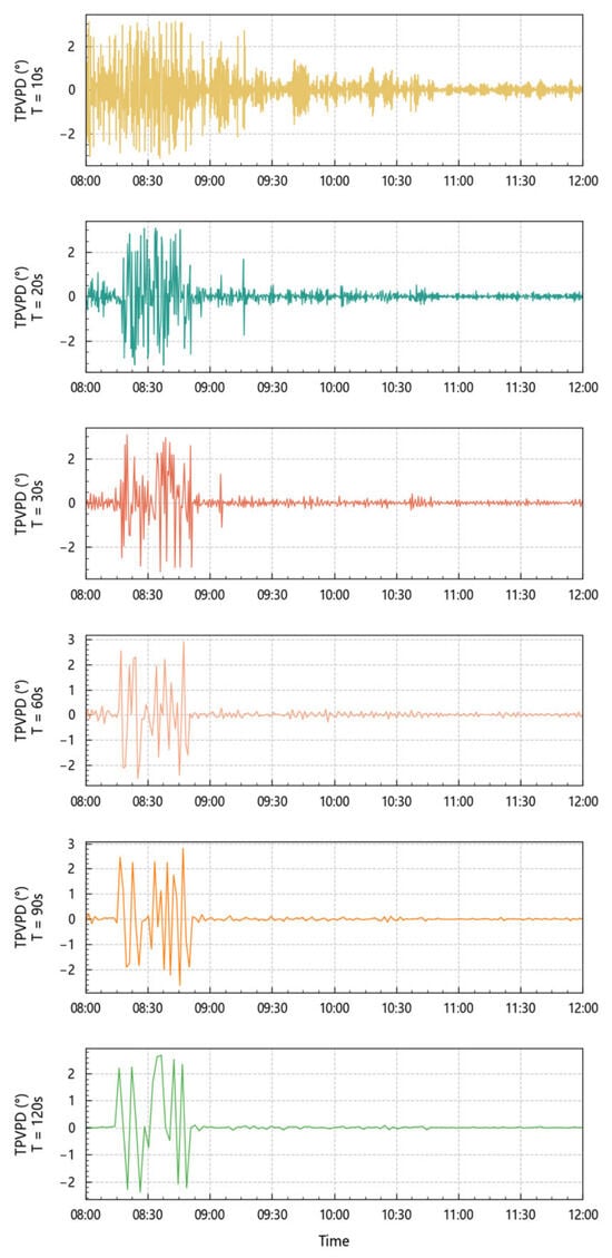
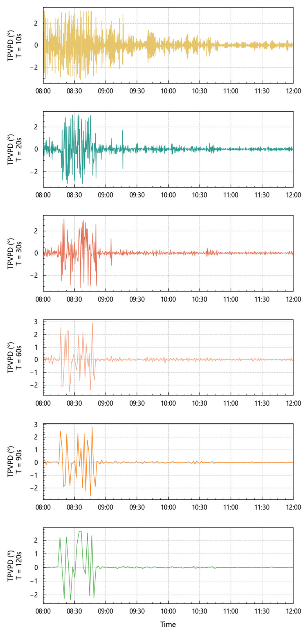
The window length T used in the TPVPD calculation is an important hyperparameter. A larger window length reduces the influence of noise and yields more stable phase estimates, but at the cost of lower temporal resolution; conversely, a smaller window length improves temporal resolution but increases the phase-estimation variance. For a harmonic component of frequency f, a T-second window contains fT cycles, so T must be large enough for a reliable phase estimate even at the lowest VIV frequency (0.183 Hz). The effects of different window lengths are illustrated in Figure 8. In addition, a quantitative comparison was performed by repeating the complete identification procedure of Section 3.4 with T = 10, 30, and 60 s for all six annual datasets; the pooled window-level F1 score amounts to 0.78 for T = 10 s, 0.77 for T = 30 s, and 0.84 for T = 60 s, and T = 60 s also yields the most stable results across individual years. At T = 60 s, even the lowest VIV mode completes about eleven cycles per window, which is sufficient for stable phase estimation. Considering the trade-off between estimation stability, temporal resolution, and detection latency, T = 60 s was adopted in this study.
Figure 8.
Comparison of different T values.
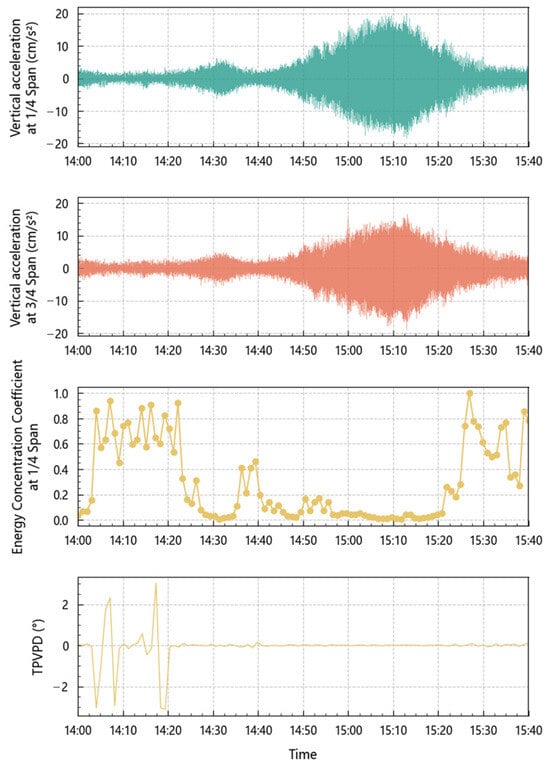
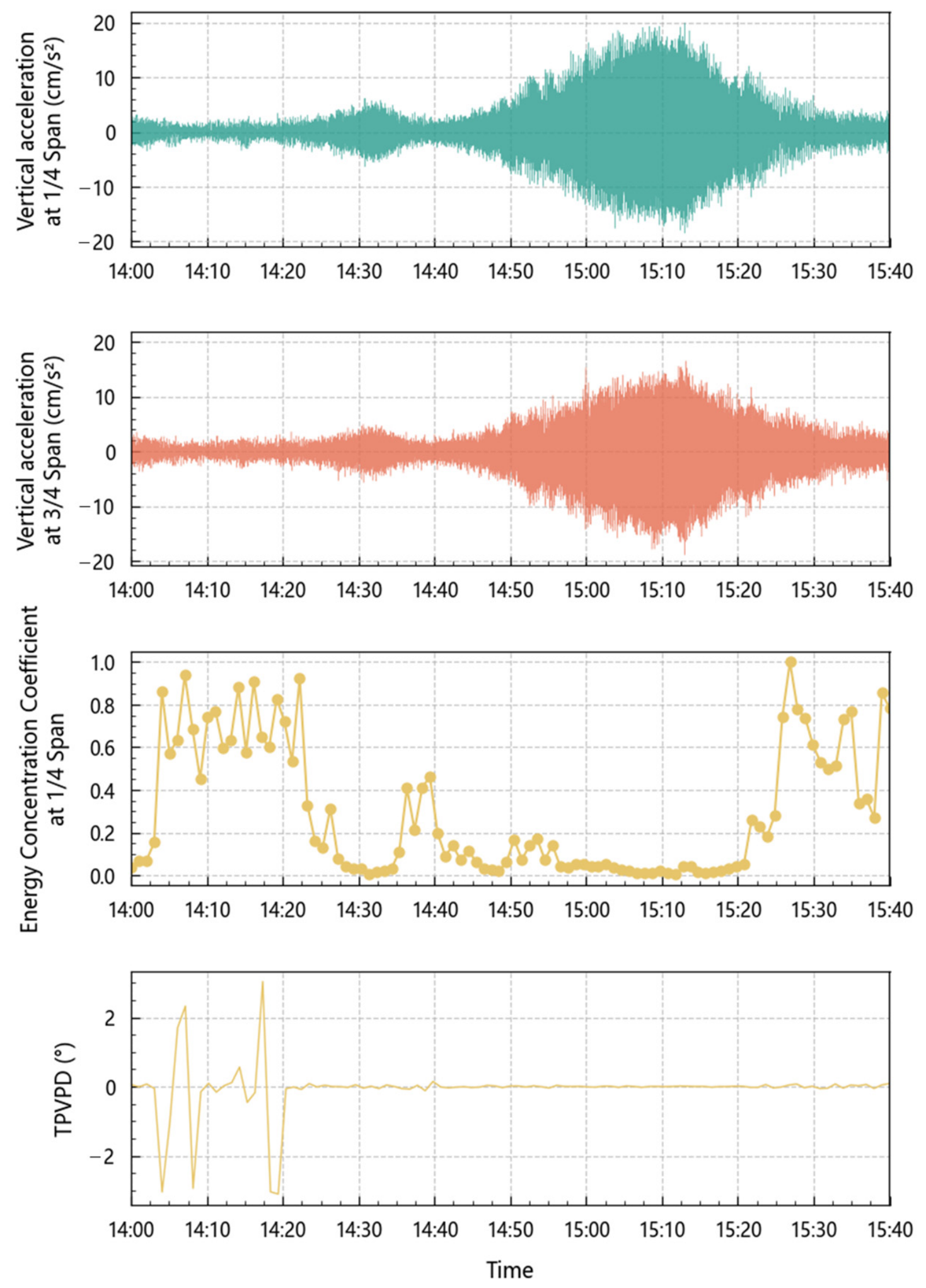
Previous studies have widely employed frequency-domain indicators to characterize the single-frequency nature of vibration responses, which represents a key feature of VIV. In this study, the energy concentration coefficient (ECC) proposed by Li et al. [18] is adopted, and its formal definition is given as follows. For each 10-min acceleration record, the power spectral density is estimated by the Welch method with a Hann window, 50% segment overlap, and a frequency resolution of 1/600 Hz, restricted to the range 0.05–1 Hz; I1 denotes the largest local spectral peak and I2 the highest peak separated from the dominant peak by more than 0.02 Hz. The ECC is defined as ECC = I2/I1, such that a strictly single-frequency signal yields ECC → 0, whereas broadband responses yield larger values; for VIV windows the ECC is generally below 0.1. However, such indicators are primarily derived from frequency-domain statistics of single-point signals and may exhibit limited responsiveness to transient variations during the early stage of VIV development. From a complementary perspective, the proposed TPVPD focuses on the spatial coordination of structural vibrations by tracking phase consistency between different measurement points, making it more sensitive to the onset of VIV. As illustrated in Figure 9, a direct comparison between ECC and TPVPD for a representative VIV event shows that TPVPD converges earlier at the initial stage, thereby providing information that effectively complements the steady-state representation offered by ECC.
Figure 9.
Comparison between ECC and TPVPD.
3.4. Automatic Identification of VIVs Based on Spectral Clustering and TPVPD
To achieve automatic identification of vortex-induced vibration (VIV) events, the proposed TPVPD parameter is integrated with a spectral clustering algorithm. The long-term monitoring data are first segmented into 10-min time windows, within which statistical features are extracted to construct a feature dataset for clustering analysis. Three representative features are selected as the clustering inputs:
- (1)
- Arms1: The root mean square (RMS) of acceleration at the 1/4-span location. For a given vibration mode, the acceleration amplitudes at the 1/4- and 3/4-span locations maintain an approximately constant ratio. Therefore, Arms1 alone is sufficient to characterize the vibration amplitude, and Arms3 does not provide additional effective information;
- (2)
- Standard deviation of TPVPD: This feature reflects the temporal stability of the phase difference within each 10-min window. Considering that the calculation window of TPVPD is T = 60 s, each 10-min segment contains 10 TPVPD values. Their standard deviation quantitatively describes the temporal fluctuation of vibration synchronism;
- (3)
- Energy concentration coefficient (ECC): This parameter characterizes the energy concentration of each 10-min vibration signal [18]. Due to the pronounced single-frequency characteristic of VIV signals, the ECC value is generally lower than 0.1.
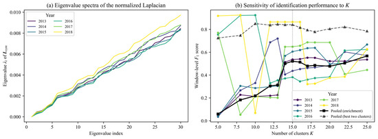
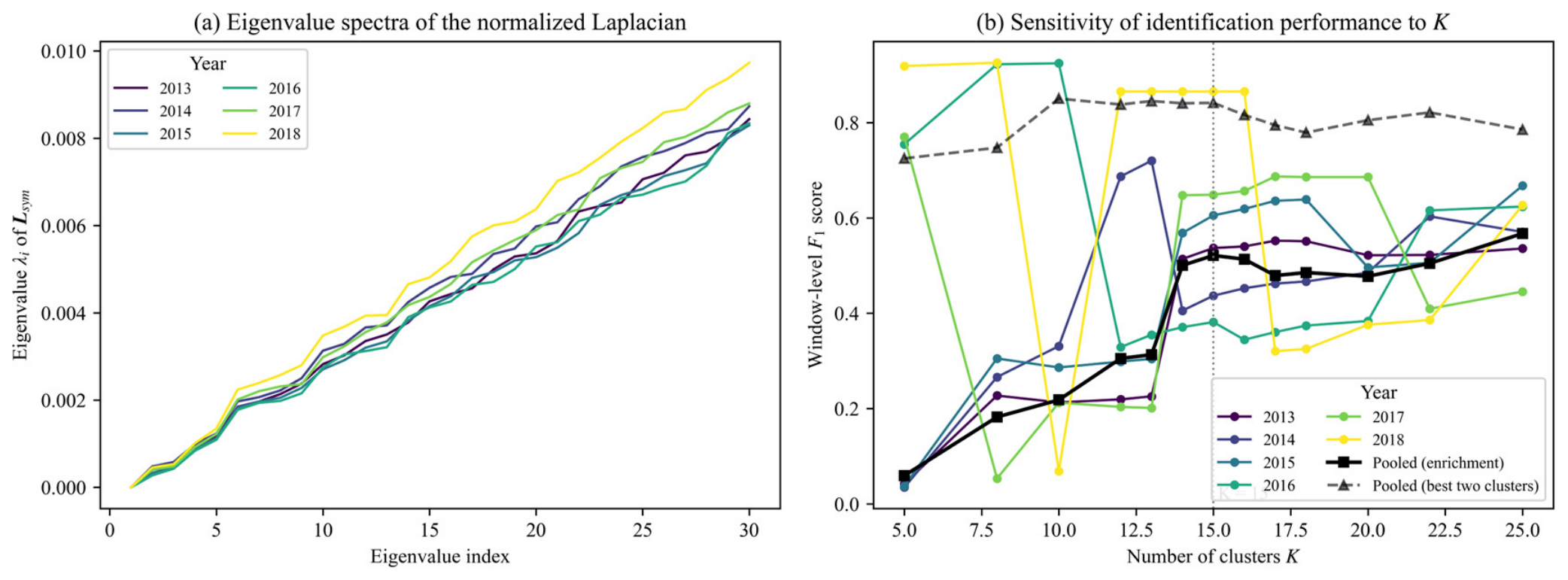
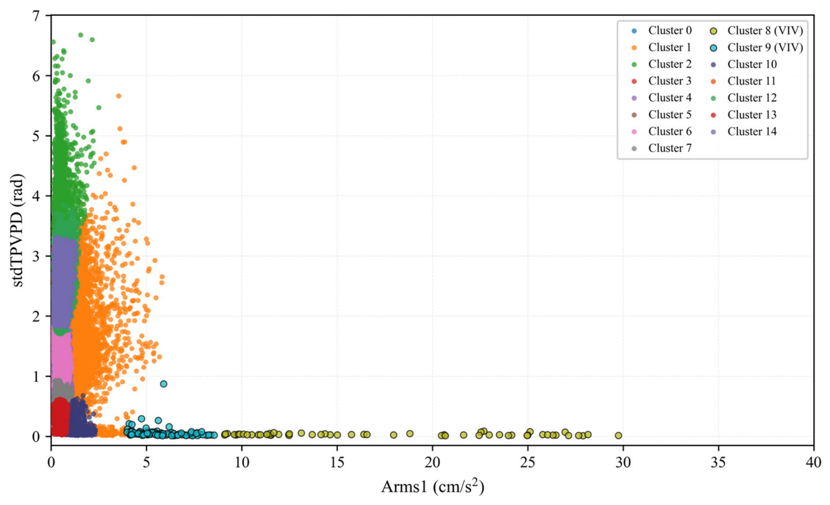
Based on these features, spectral clustering was conducted separately for each annual dataset with the number of clusters set to K = 15. Since K directly determines the granularity of the VIV/non-VIV boundary, its selection is documented explicitly here. Figure 10a shows the eigenvalue spectra of the normalized graph Laplacian for the six annual datasets; the eigenvalues decay smoothly without a single pronounced eigen-gap, which is typical for continuous monitoring data whose clusters overlap in feature space. Therefore, K was determined by a sensitivity study: the complete identification procedure was repeated for K = 5–25 for all six years, and the window-level agreement with the reference VIV inventory (Section 3.5) remains within a plateau of F1 = 0.82–0.85 for K between 10 and 16 (Figure 10b). Within this plateau, K = 15 was adopted because it provides sufficient granularity to separate the different VIV stages and modes while keeping the clusters physically interpretable; larger values fragment the small VIV clusters and reduce interpretability without improving performance, whereas smaller values merge transitional VIV states into the buffeting background.
Figure 10.
Selection of the number of clusters K: (a) eigenvalue spectra of the normalized graph Laplacian for the six annual datasets; (b) window-level F1 score versus K pooled over 2013–2018, evaluated against the reference VIV inventory (mapping definitions in Section 3.5); the adopted K = 15 is indicated.
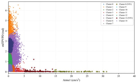
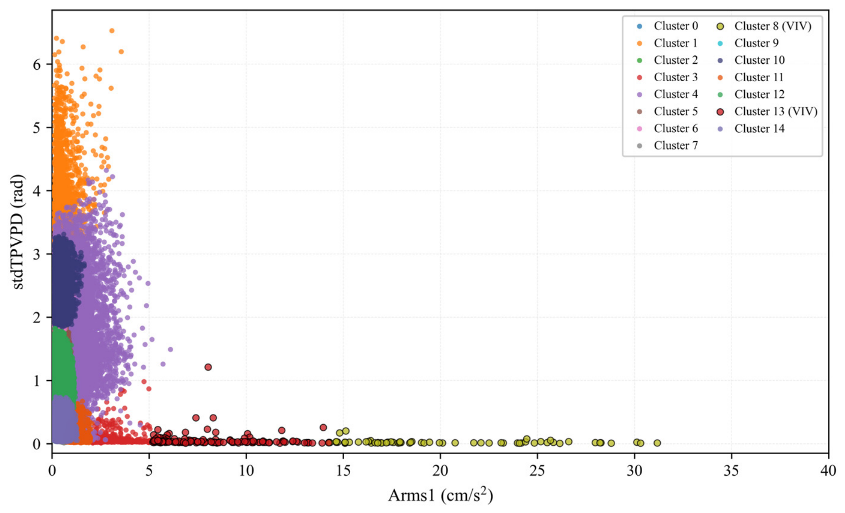
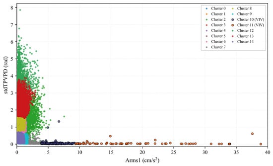
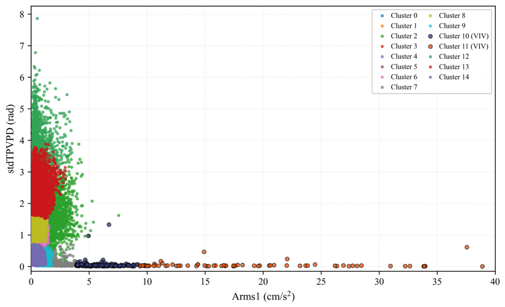
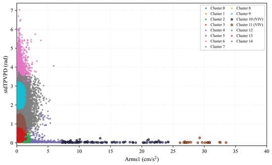
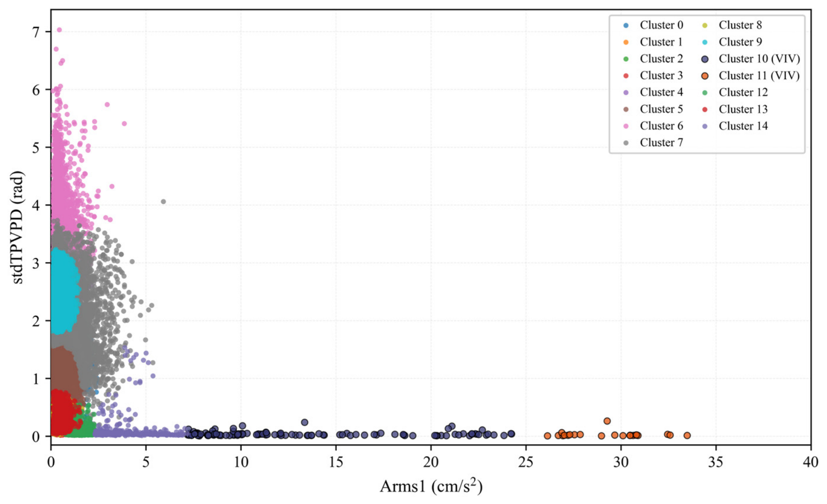
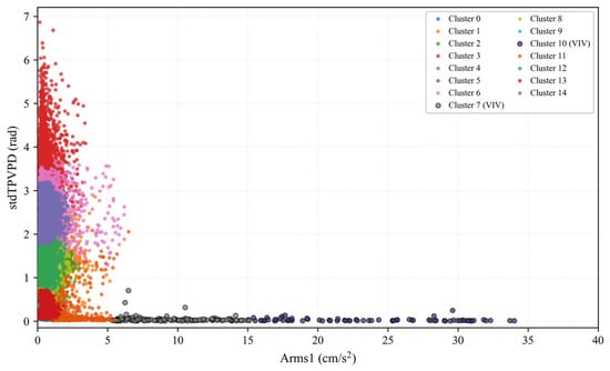
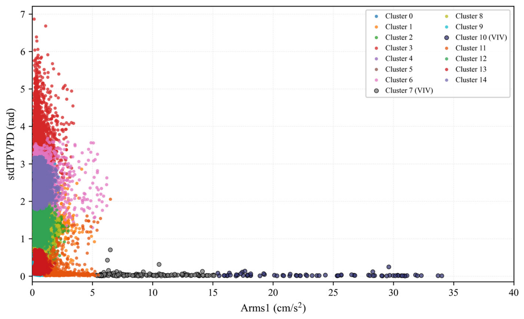
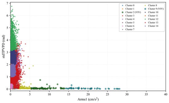
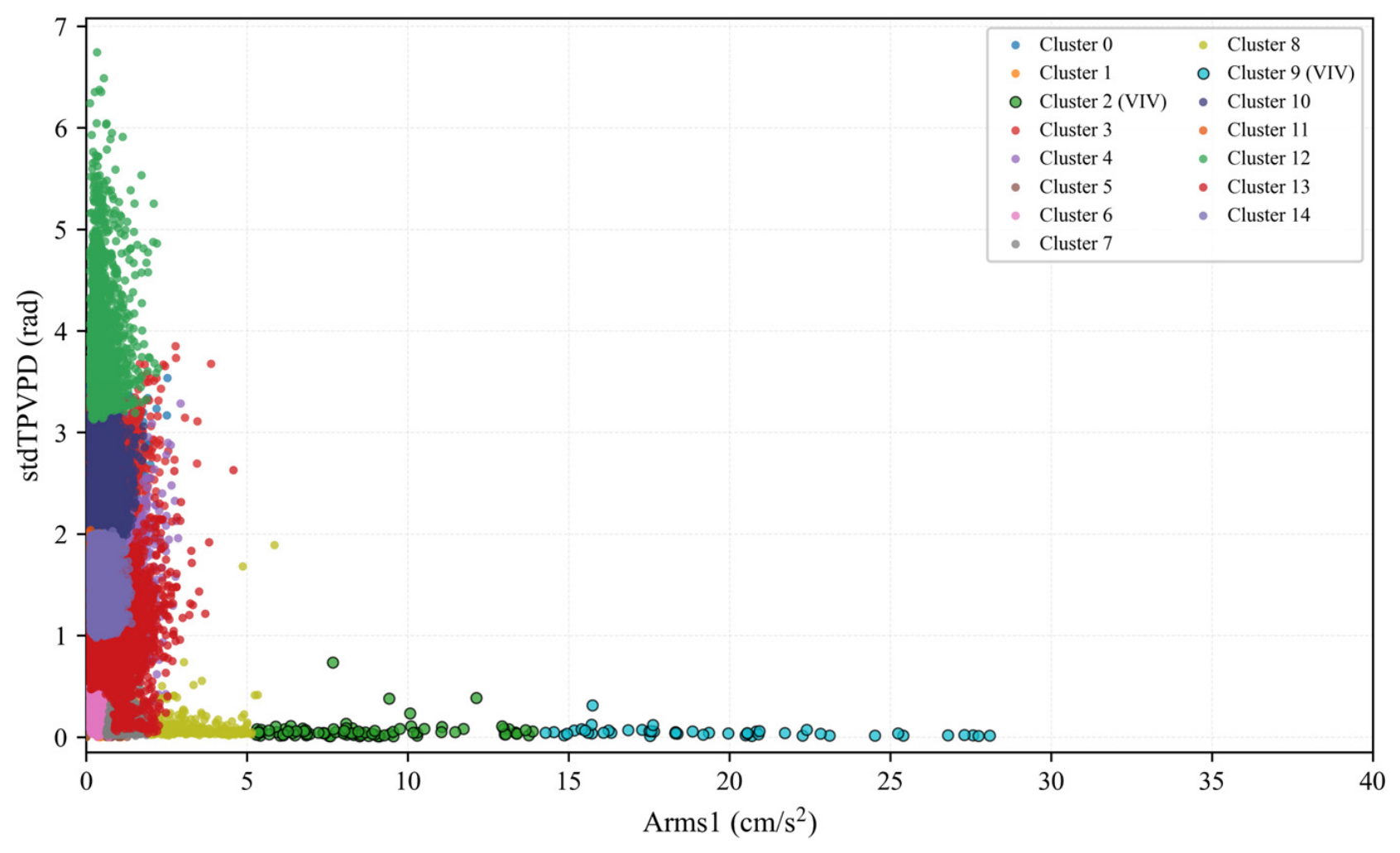
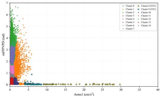
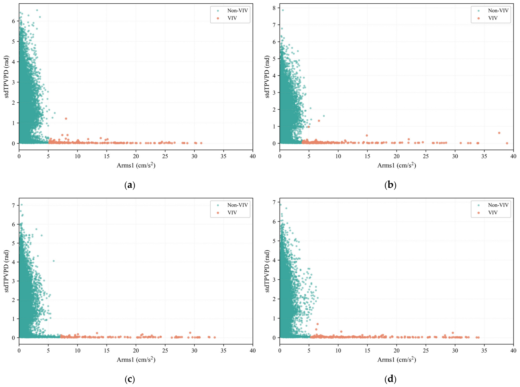
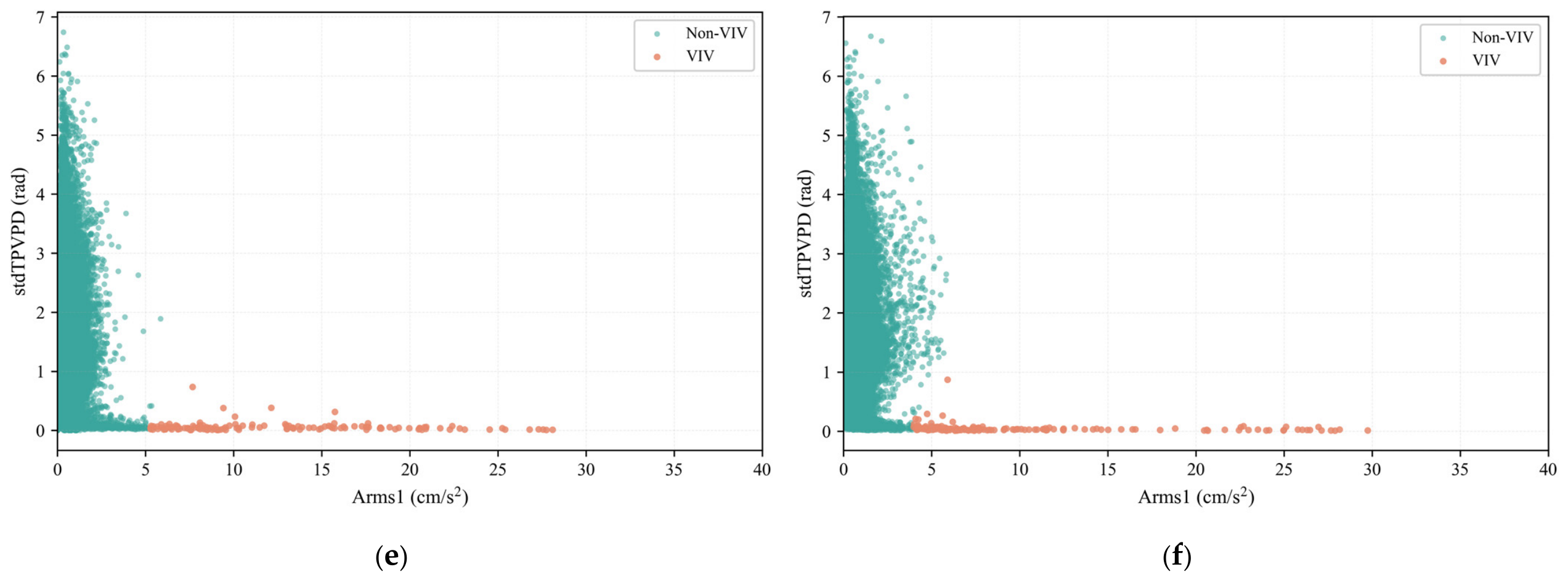
Due to the extremely large size of the long-term monitoring dataset, directly applying clustering analysis to the entire dataset would not only significantly reduce computational efficiency, but also obscure the differences in wind environment and structural dynamic characteristics among different years, thereby degrading the discriminative capability and interpretability of the clustering results. To address this issue, the monitoring data from 2013 to 2018 were divided on an annual basis, resulting in six independent datasets corresponding to the years 2013, 2014, 2015, 2016, 2017, and 2018. Spectral clustering was then applied separately to each annual dataset, and the corresponding clustering results are shown in Figure 11, Figure 12, Figure 13, Figure 14, Figure 15 and Figure 16.
Figure 11.
Clustering results of year 2013.
Figure 12.
Clustering results of year 2014.
Figure 13.
Clustering results of year 2015.
Figure 14.
Clustering results of year 2016.
Figure 15.
Clustering results of year 2017.
Figure 16.
Clustering results of year 2018.
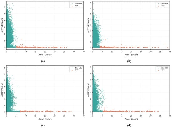
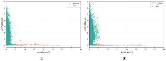
After implementation of the spectral clustering procedure described in Section 2.2 (z-score feature normalization, kNN graph construction with k = 10, Laplacian eigendecomposition, and k-means assignment in the embedding space), the clustering results of each year were interpreted by examining representative vibration time histories and spectra of every cluster. Clusters exhibiting typical VIV characteristics (large amplitude, a single dominant frequency, and a stable TPVPD) were designated as VIV clusters and the remainder as non-VIV clusters. This designation was performed once per annual dataset and is summarized in Table 2; the corresponding classification results are shown in Figure 17. It is emphasized that the reference VIV inventory used for the quantitative validation in Section 3.5 was compiled independently of the present method, following the cluster-analysis-based identification strategy of Li et al. [18] combined with inspection of the original vibration records; it was not used at any stage of feature extraction, clustering, or cluster designation. For operational use, an explicit automated rule that reproduces this designation is introduced in Section 3.5, so that new monitoring windows can be classified without repeating the manual annual analysis.
Table 2.
Cluster designation schemes for each annual dataset.
Figure 17.
VIV classification results: (a) Year 2013; (b) Year 2014; (c) Year 2015; (d) Year 2016; (e) Year 2017; (f) Year 2018.
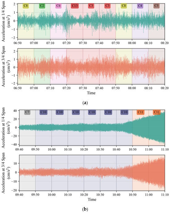
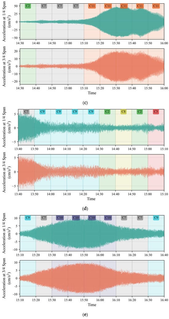
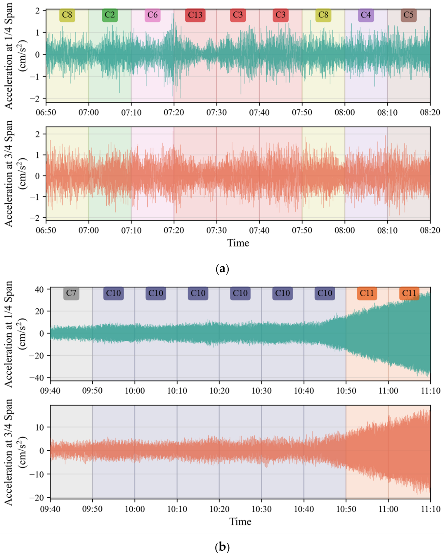
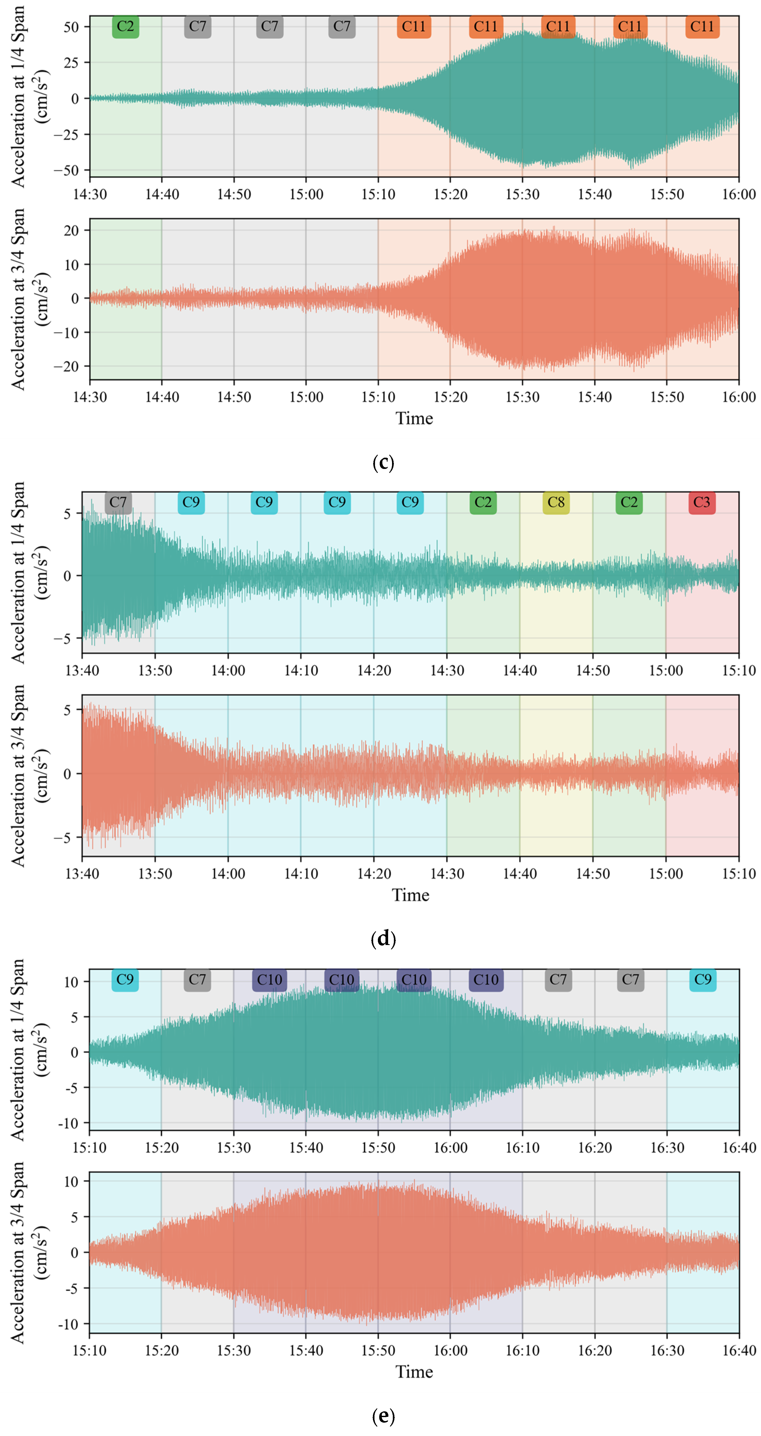
To further investigate the physical significance of the spectral clustering results, the data from 2014 were selected as a representative example. Typical samples from different clusters were extracted and analyzed in detail, as shown in Figure 18. Clear differences can be observed among the clusters in terms of vibration amplitude, spectral characteristics, and TPVPD stability, indicating a strong correspondence between the spectral clustering results and the actual dynamic responses of the bridge under different wind-induced vibration states.
Figure 18.
Typical samples of different clusters in 2014 (vertical acceleration at the 1/4- and 3/4-span positions, with the cluster label of each 10-min window annotated): (a) typical non-VIV (buffeting) windows, with small amplitudes and broadband spectra; (b) weak and transitional VIV windows; (c) initiation and growth stage of a VIV event; (d) steady, large-amplitude VIV state; (e) decay stage of a VIV event returning to buffeting.
Clusters 0, 1, 2, 3, 4, 5, 6, 8, 12, 13, and 14 are identified as typical non-VIV samples. These samples are primarily associated with buffeting responses induced by the turbulent components of the incoming wind. They are characterized by small vibration amplitudes, broadband frequency content with dispersed energy, and unstable TPVPD values, indicating a lack of stable phase synchronization between measurement points.
Clusters 7 and 9 correspond to extremely small-amplitude VIV states or transitional conditions from buffeting to VIV. Such cases typically occur when the wind speed is close to the boundary of the VIV lock-in region, where only weak structural responses can be excited. Although the vibration amplitudes are relatively small, the frequency spectra already exhibit certain single-frequency characteristics, and the TPVPD shows a higher degree of convergence compared with pure buffeting states. Because these clusters contain a mixture of weak VIV and ordinary buffeting windows, they were conservatively designated as non-VIV in the strict scheme of Table 2. The impact of this choice was quantified by repeating the evaluation with clusters 7 and 9 included in the VIV class: the recall increases from 0.93 to 0.97, but the false-positive rate increases sharply from 0.11% to 3.67% (the number of false-positive windows grows from 48 to 1635). The strict designation therefore offers a balanced treatment of transitional states, at the cost of a small number of missed weak-VIV windows; the missed windows are further examined in Section 3.5.
Cluster 10 can be regarded as a small-amplitude VIV state, or as the initiation stage or late decay stage of a large-amplitude VIV event. While the overall vibration amplitude remains relatively small, a clear dominant frequency is present in the spectrum, and the TPVPD becomes stable, indicating that the structure has entered or is about to exit a typical VIV state.
Cluster 11 represents a standard large-amplitude VIV state, characterized by significantly increased vibration amplitudes, highly concentrated spectral energy at a single dominant frequency, and a highly stable TPVPD. This reflects the formation of a stable synchronized vibration pattern of the structure under VIV.
These results demonstrate that the feature space constructed using Arms1, ECC, and the standard deviation of TPVPD, combined with the spectral clustering method, not only enables effective discrimination between VIV and non-VIV responses, but also allows further identification of different stages in the evolution of VIV. The quantitative validation of these results, the contribution of the TPVPD feature, and an automated cluster-assignment rule are presented in Section 3.5.
3.5. Quantitative Validation and Operational Application
The agreement between the identification results and the reference VIV inventory was assessed at the 10-min window level over the 284,897 valid windows of 2013–2018 (about 9.7% of the nominal 315,360 10-min slots were discarded because of missing data). The reference inventory was compiled by the authors independently of the present method, following the cluster-analysis-based identification strategy of Li et al. [18] and inspection of the original vibration records, and was never used in feature extraction, clustering, or cluster designation. Table 3 lists the confusion-matrix entries and the derived metrics for each year and for the pooled dataset. Over the six years, 975 of the 1236 reference VIV windows were correctly identified (recall 0.789) with 108 false-positive windows (precision 0.900, F1 = 0.841, false-positive rate 0.038%). The recall varies among years (0.60–0.96) because a fraction of the reference windows correspond to weak or transitional VIV states, which the strict cluster designation deliberately excludes (see the discussion of clusters 7 and 9 in Section 3.4), whereas the precision remains high (0.79–0.99) in all years. It should be emphasized that the reference inventory is itself derived from a cluster-analysis-based identification and therefore inherits a degree of uncertainty; the metrics should thus be interpreted as agreement with an independently compiled reference rather than as accuracy against an absolute ground truth, and all 369 disagreement windows were additionally verified against the original vibration records and spectra.
Table 3.
Window-level agreement between the identification results and the reference VIV inventory (strict designation of Table 2).
As a validation that does not rely on the reference inventory, the dominant spectral peak of every window classified as VIV was computed from the raw acceleration records and compared with the six documented VIV mode frequencies of the bridge (Table 1). In total, 1081 of the 1083 windows classified as VIV (99.8%) have their spectral peak within ±0.01 Hz of one of the six mode frequencies, and all six modes are represented (Table 1). Notably, 98% of the 108 windows that disagree with the reference inventory also exhibit mode-aligned spectral peaks, suggesting that most of them correspond to genuine weak-VIV or transitional states that are missing from the reference inventory; the same holds for 99% of the 261 missed windows. These findings were further checked by manual inspection of the original time histories and spectra of all disagreement windows.
To isolate the contribution of TPVPD, an ablation study was performed in which the complete procedure (z-score normalization, spectral clustering with K = 15, and cluster-to-class assignment) was repeated with five feature sets: RMS only, ECC only, RMS + ECC, RMS + TPVPD, and RMS + TPVPD + ECC. Two cluster-to-class mapping rules were applied identically to all feature sets: an automatic enrichment rule, in which a cluster is labeled VIV if the fraction of reference VIV windows within it exceeds the annual base rate; and an upper-bound rule, in which the best pair of clusters—analogous to the manual designation of Table 2—is selected to maximize the F1 score. Table 4 reports the pooled results for 2013–2018. With RMS or ECC alone, the VIV windows are scattered across clusters and the identification essentially fails (F1 ≤ 0.05). RMS + ECC attains a high precision but misses about 44% of the reference VIV windows (recall 0.558), because weak and early-stage VIV states cannot be separated from the buffeting background by single-point spectral concentration alone. Replacing ECC by TPVPD raises the recall to 0.751, and the full feature set further improves the F1 score to 0.841 with a recall of 0.790—identical to the manually designated scheme of Table 2. These results quantify the specific contribution of TPVPD: it is primarily responsible for recovering the weak and transitional VIV states that single-point frequency-domain indicators miss.
Table 4.
Ablation study of the clustering features (pooled over 2013–2018; FPR = false-positive rate).
To complete the automation chain and to examine cross-year transferability, an explicit rule was calibrated to assign new samples to the VIV and non-VIV classes without repeating the manual annual analysis. Using the designation of Table 2, the centroids of the VIV and non-VIV windows in the z-scored feature space are computed from the calibration years. A new 10-min window, after normalization with the same calibration statistics, is classified as VIV if it lies closer to the VIV centroid than to the non-VIV centroid. Table 5 lists the results of a chronological cross-year validation in which the rule was calibrated on all previous years and applied to the subsequent year. On the five unseen years, the rule attains a precision of 0.96–0.99 with a false-positive rate below 0.02%, and an F1 score between 0.74 and 0.88 (mean 0.82), which approaches the performance of the per-year clustering with manual designation (pooled F1 = 0.841, Table 3). During bridge operation, the clustering-based designation can therefore be replaced by this simple and transparent classification rule. The detection latency of the operational workflow is dominated by the 10-min classification interval—the 60-s TPVPD sub-windows and the feature extraction require only a few seconds of computation—so an event can be detected within at most about 10 min of its occurrence; claims regarding real-time early warning should be interpreted with this latency in mind.
Table 5.
Cross-year validation of the automated nearest-centroid assignment rule (window level, against the reference VIV inventory).
4. Conclusions
This study presented a field-oriented method for identifying vortex-induced vibration (VIV) events in long-span bridges by integrating a newly proposed Two-Point Vibration Phase Difference (TPVPD) feature with spectral clustering. Unlike conventional VIV identification approaches that rely primarily on single-point vibration indicators or supervised learning with manually labeled samples, the proposed framework exploits the phase-synchronization characteristics of single-mode-dominated responses measured at two spatially separated locations along the bridge span, enabling robust unsupervised identification under realistic monitoring conditions, complemented by an explicit rule-based cluster assignment for operational use.
From a theoretical perspective, TPVPD is derived from modal vibration theory and reflects the time-invariant phase relationship between different points of a structure responding in a single dominant mode. This property distinguishes single-mode-dominated VIV from buffeting-dominated responses, which lack stable spatial phase coherence: during an analyzed VIV event the mean 10-min TPVPD standard deviation was 1.6°, against 126.5° during a strong buffeting episode. TPVPD should be interpreted as a useful indicator of single-mode-dominated responses rather than an exclusive signature of VIV, and therefore used in combination with amplitude and spectral features. Compared with traditional frequency-domain indicators such as the ECC, TPVPD exhibits higher sensitivity to the onset of VIV and provides higher temporal resolution, as quantified by the ablation study (recall 0.558 with RMS + ECC versus 0.790 with the full feature set).
Based on six years (2013–2018) of long-term field monitoring data from a 1650-m main-span suspension bridge (284,897 valid 10-min windows), the TPVPD-based feature set—acceleration RMS, TPVPD standard deviation, and ECC—was combined with spectral clustering to analyze massive unlabeled datasets. VIV and non-VIV responses were effectively separated without prior labeling (pooled window-level F1 = 0.841 against a reference VIV inventory, with a precision of 0.900 and a false-positive rate of 0.038%), and different VIV states, including initiation, steady-state, and decay phases, were further distinguished. All six known VIV modes of the bridge were identified, and 99.8% of the windows classified as VIV exhibited spectral peaks within ±0.01 Hz of one of the six documented mode frequencies. A rule-based assignment calibrated on previous years transferred to subsequent years with F1 scores of 0.74–0.88, supporting operational deployment.
Several limitations should be noted. The framework identifies VIV at the 10-min window level, so the reported detection latency is bounded by the 10-min classification interval rather than being instantaneous. The validation metrics quantify agreement with a reference inventory that was itself compiled by a cluster-analysis-based procedure; although a physical frequency check was performed and all disagreement windows were manually inspected against the original records, a fully independent benchmark is not yet available. The two-side averaging of the vertical accelerations neglects torsional effects, and the rule-based assignment and the selection of K were validated on a single bridge; cross-bridge generalization deserves further study.
Overall, the proposed TPVPD–spectral clustering framework provides an efficient, robust, and scalable solution for long-term VIV identification in long-span bridges. It reduces reliance on wind tunnel tests and manual data inspection and enhances adaptability to complex natural wind environments. Future work will focus on improving the temporal precision of VIV identification (sub-interval onset and termination detection), incorporating torsional responses, extending the framework to other bridges and to vibration state evolution analysis, and developing practical early-warning applications with explicit latency budgets.
Author Contributions
Conceptualization, S.L.; methodology, Y.X. and N.X.; software, Y.X. and N.X.; validation, D.W., N.X. and Y.Z.; formal analysis, Y.X. and N.X.; investigation, Y.Z. and N.X.; resources, D.W.; data curation, N.X.; writing—original draft preparation, D.W., N.X. and Y.X.; writing—review and editing, D.W., N.X. and S.L.; visualization, Y.X. and N.X.; supervision, S.L. and W.C.; project administration, S.L. and W.C.; funding acquisition, S.L. All authors have read and agreed to the published version of the manuscript.
Funding
This study is financially supported by the National Key Research and Development Program of China under grant No. 2022YFC3005303.
Institutional Review Board Statement
Not applicable.
Informed Consent Statement
Not applicable.
Data Availability Statement
The extracted 10-min feature datasets, the reference VIV inventory, and the core code implementing the proposed method are available from the corresponding author upon reasonable request, together with representative sample data to support reproducibility. The raw acceleration monitoring records are available from the corresponding author upon reasonable request.
Conflicts of Interest
Author Du Wu was employed by the company CCCC Highway Consultants Co., Ltd. Authors Yichao Xu and Yufeng Zhang were employed by the company JSTI Group. The remaining authors declare that the research was conducted in the absence of any commercial or financial relationships that could be construed as a potential conflict of interest.
Abbreviations
The following abbreviations are used in this manuscript:
| VIV | Vortex-induced vibration |
| SHM | structural health monitoring |
| TPVPD | Two-Point Vibration Phase Difference |
| CFD | computational fluid dynamics |
| RMS | root-mean-square |
| ECC | Energy Concentration Coefficient |
| SVM | support vector machine |
References
- Kumarasena, T.; Scanlan, R.H.; Morris, G.R. Deer Isle Bridge: Field and Computed Vibrations. J. Struct. Eng. 1989, 115, 2313–2328. [Google Scholar] [CrossRef] [Scilit]
- Smith, I.J. Wind Induced Dynamic Response of the Wye Bridge. Eng. Struct. 1980, 2, 202–208. [Google Scholar] [CrossRef] [Scilit]
- Weber, F.; Maślanka, M. Frequency and Damping Adaptation of a TMD with Controlled MR Damper. Smart Mater. Struct. 2012, 21, 055011. [Google Scholar] [CrossRef] [Scilit]
- Fujino, Y.; Yoshida, Y. Wind-Induced Vibration and Control of Trans-Tokyo Bay Crossing Bridge. J. Struct. Eng. 2002, 128, 1012–1025. [Google Scholar] [CrossRef] [Scilit]
- Zhao, L.; Cui, W.; Shen, X.; Xu, S.; Ding, Y.; Ge, Y. A Fast On-Site Measure-Analyze-Suppress Response to Control Vortex-Induced-Vibration of a Long-Span Bridge. Structures 2022, 35, 192–201. [Google Scholar] [CrossRef] [Scilit]
- Dan, D.; Wang, C.; Shi, H.; Ge, L. Gaussian Process Regression Prediction Model for Vortex-Induced Vibration of Suspension Bridges Driven by Real Bridge Monitoring Data. ASCE-ASME J. Risk Uncertain. Eng. Syst. Part A Civ. Eng. 2025, 11, 04025068. [Google Scholar] [CrossRef] [Scilit]
- Kwok, K.C.S.; Qin, X.R.; Fok, C.H.; Hitchcock, P.A. Wind-Induced Pressures around a Sectional Twin-Deck Bridge Model: Effects of Gap-Width on the Aerodynamic Forces and Vortex Shedding Mechanisms. J. Wind Eng. Ind. Aerodyn. 2012, 110, 50–61. [Google Scholar] [CrossRef] [Scilit]
- Trein, C.A.; Shirato, H.; Matsumoto, M. On the Effects of the Gap on the Unsteady Pressure Characteristics of Two-Box Bridge Girders. Eng. Struct. 2015, 82, 121–133. [Google Scholar] [CrossRef] [Scilit]
- Lee, S.; Kwon, S.-D.; Yoon, J. Reynolds Number Sensitivity to Aerodynamic Forces of Twin Box Bridge Girder. J. Wind Eng. Ind. Aerodyn. 2014, 127, 59–68. [Google Scholar] [CrossRef] [Scilit]
- Ma, R.; Li, F.; Hu, X.; Ge, B.; He, Q. Experiment Study on Vortex-Induced Vibration of a Twin-Box Girder with Large Cantilever Plates. Structures 2023, 55, 891–907. [Google Scholar] [CrossRef] [Scilit]
- Diana, G.; Resta, F.; Belloli, M.; Rocchi, D. On the Vortex Shedding Forcing on Suspension Bridge Deck. J. Wind Eng. Ind. Aerodyn. 2006, 94, 341–363. [Google Scholar] [CrossRef] [Scilit]
- Xue, G.; Laima, S. Quantitative Relationship between Hydrodynamic Forces and Flow Structures for Rectangular Cylinders with Varying Aspect Ratios. Ocean Eng. 2026, 357, 125612. [Google Scholar] [CrossRef] [Scilit]
- Laima, S.; Zhang, L.; Xue, G.; Chen, W.; Li, H. Investigation of Vortex-Induced Vibration Response of Rectangular Prisms with Various Aspect Ratios. Phys. Fluids 2026, 38, 045129. [Google Scholar] [CrossRef] [Scilit]
- Larsen, A.; Esdahl, S.; Andersen, J.E.; Vejrum, T. Storebælt Suspension Bridge—Vortex Shedding Excitation and Mitigation by Guide Vanes. J. Wind Eng. Ind. Aerodyn. 2000, 88, 283–296. [Google Scholar] [CrossRef] [Scilit]
- Frandsen, J.B. Simultaneous Pressures and Accelerations Measured Full-Scale on the Great Belt East Suspension Bridge. J. Wind Eng. Ind. Aerodyn. 2001, 89, 95–129. [Google Scholar] [CrossRef] [Scilit]
- Buka-Vaivade, K.; Nicoletti, V.; Gara, F. Advancing Bridge Resilience: A Review of Monitoring Technologies for Flood-Prone Infrastructure. Open Res. Eur. 2025, 5, 26. [Google Scholar] [CrossRef] [Scilit] [PubMed]
- Liu, J.Q.; Bai, B.C.; Liu, R.H.; Li, W.J.; Zhao, X.F. Lightweight and Hierarchical Adaptive Strain Monitoring for Bridges Based on Microscopic Vision Sensing. Comput.-AIDED Civ. Infrastruct. Eng. 2026, 47. [Google Scholar] [CrossRef] [Scilit]
- Li, S.; Laima, S.; Li, H. Cluster Analysis of Winds and Wind-Induced Vibrations on a Long-Span Bridge Based on Long-Term Field Monitoring Data. Eng. Struct. 2017, 138, 245–259. [Google Scholar] [CrossRef] [Scilit]
- Xu, S.; Ma, R.; Wang, D.; Chen, A.; Tian, H. Prediction Analysis of Vortex-Induced Vibration of Long-Span Suspension Bridge Based on Monitoring Data. J. Wind Eng. Ind. Aerodyn. 2019, 191, 312–324. [Google Scholar] [CrossRef] [Scilit]
- Huang, Z.; Li, Y.; Hua, X.; Chen, Z.; Wen, Q. Automatic Identification of Bridge Vortex-Induced Vibration Using Random Decrement Method. Appl. Sci. 2019, 9, 2049. [Google Scholar] [CrossRef] [Scilit]
- He, M.; Liang, P.; Zhang, Y.; Wang, Y.; Wang, K. Identification, Tracking and Warning of Vortex Induced Vibration Using k-Means Clustering Method. Struct. Infrastruct. Eng. 2024, 20, 380–393. [Google Scholar] [CrossRef] [Scilit]
- Hou, J.; Cao, S.; Hu, H.; Zhou, Z.; Wan, C.; Noori, M.; Li, P.; Luo, Y. Vortex-Induced Vibration Recognition for Long-Span Bridges Based on Transfer Component Analysis. Buildings 2023, 13, 2012. [Google Scholar] [CrossRef] [Scilit]
- Kim, S.; Kim, T. Machine-Learning-Based Prediction of Vortex-Induced Vibration in Long-Span Bridges Using Limited Information. Eng. Struct. 2022, 266, 114551. [Google Scholar] [CrossRef] [Scilit]
- Lim, J.; Kim, S.; Kim, H.-K. Using Supervised Learning Techniques to Automatically Classify Vortex-Induced Vibration in Long-Span Bridges. J. Wind Eng. Ind. Aerodyn. 2022, 221, 104904. [Google Scholar] [CrossRef] [Scilit]

Disclaimer/Publisher’s Note: The statements, opinions and data contained in all publications are solely those of the individual author(s) and contributor(s) and not of MDPI and/or the editor(s). MDPI and/or the editor(s) disclaim responsibility for any injury to people or property resulting from any ideas, methods, instructions or products referred to in the content. |
© 2026 by the authors. Licensee MDPI, Basel, Switzerland. This article is an open access article distributed under the terms and conditions of the Creative Commons Attribution (CC BY) license.