Benchmarking Deformable-Attention Graph Networks and Other Aggregators on Prov-GigaPath Features for Canine Cutaneous Tumor Classification

Abstract

Whole-slide image (WSI) classification in veterinary computational pathology usually freezes a human-pretrained pathology foundation model as the tile encoder and trains a light slide-level aggregator on top. Whether the choice of aggregator matters for small canine cohorts has not been tested under a common protocol. On the public CATCH dataset (350 canine cutaneous tumor WSIs, seven subtypes), we compared 14 aggregators that shared frozen Prov-GigaPath tile embeddings, patient-level five-fold splits, and training budgets: multiple-instance learning (MIL) poolings (including ACMIL), static-graph and dynamic-graph neural networks (GNNs, including WiKG), and GigaPath-DefGNN, a coordinate-aware deformable graph-attention aggregator that we adapted to tile point clouds of up to ~94,000 tiles. On the held-out test partitions, pooled over all 350 WSIs, the 14 aggregators spanned a balanced accuracy of 0.889–0.960. GigaPath-DefGNN reached 0.940 (95% confidence interval 0.910–0.967) with best-validation checkpoints and did not differ significantly from any baseline (exact McNemar tests, smallest Holm-adjusted p = 0.148). Its attention maps matched pathologist tumor annotations no better than those of a graph-attention baseline (median Pearson r 0.226 versus 0.224). Validation-set estimates exceeded held-out balanced accuracy by up to 0.066, and the checkpoint-selection rule alone changed held-out accuracy by up to 0.037 and reordered the models: GigaPath-DefGNN ranked eighth under best-validation selection, first under the latest-top-3 rule, and second with the final weights of a re-run of the same configuration. Repeating the headline comparison on 20× tiles did not change these conclusions; among the graph constructions, one post hoc, exploratory variant (GigaPath-DefGNN on a feature k-nearest-neighbor graph) ranked highest. On frozen Prov-GigaPath features for this cohort, the evaluation design mattered as much as the choice of aggregator. Code, splits, and per-WSI predictions will be made publicly available.

1. Introduction

Canine cutaneous tumors are the most common neoplasm type in veterinary practice, and they span a wide histomorphological range across epithelial, mesenchymal, round-cell, and melanocytic origins. Subtype classification from hematoxylin-and-eosin (H&E) whole-slide images (WSIs) is the first step in almost every downstream clinical pipeline—prognosis estimation, treatment selection, biobank curation—and is still done almost entirely by hand. The public CATCH dataset of 350 canine cutaneous H&E whole-slide images across seven subtypes [1] is, as far as we know, the largest open benchmark for this task, and it is the substrate for this study.

Two structural constraints shape any deep-learning approach here. First, a single 40× H&E slide holds tens of thousands of diagnostically relevant 256 × 256 tile patches, so training end-to-end over all tiles is not feasible on a cohort the size of CATCH. Second, the signal a pathologist relies on—tumor architecture, invasion pattern, the spatial relation between a focal lesion and the surrounding stroma—is spatial, and no single tile carries it on its own. The common approach handles the first constraint by precomputing per-tile features with a frozen pathology foundation model and training a small slide-level aggregator on top. This separates representation cost from supervised-training cost and inherits the foundation model’s data-scale-driven representation quality.

The most widely adopted such foundation models—Prov-GigaPath [2], UNI [3], and CONCH [4]—were pretrained on hundreds of thousands of human whole-slide images. We are not aware of any public pathology foundation model pretrained specifically on canine histology. The working state of the art for veterinary computational pathology is therefore to freeze a human pretrain and train a canine head, and we follow that template. We use Prov-GigaPath, a ViT-G (Vision Transformer, giant configuration) trained with DINOv2 (self-distillation with no labels, version 2) self-supervised learning on about 1.3 billion (1,384,860,229) tiles from roughly 170,000 human WSIs across 31 tissue types, as a frozen tile encoder that produces a 1536-dimensional embedding per tile. Cross-species transfer raises a domain-shift question that the histology domain-adaptation literature has examined in detail [5,6,7]; we return to its canine implications in Section 4. The encoder is context-free at the patch level—each tile is embedded independently of its neighbors within the slide—so whichever aggregator sits downstream has to carry the spatial signal.

Two aggregator families are in common use. Multiple-instance learning (MIL) aggregators—ABMIL [8], DSMIL [9], TransMIL [10], CLAM [11], and more recent variants such as ACMIL [12]—pool tile features with attention, or attention plus clustering, and treat the WSI as an unordered bag of instances; spatial relations enter only implicitly or not at all. Graph neural networks (GNNs) over the tile cloud [13,14,15] build a graph—usually a spatial k-nearest-neighbor (k-NN) graph, a feature k-NN graph, or their union—and pass messages along fixed edges; dynamic-graph methods such as WiKG [16] instead learn the neighborhood from the features. A standard graph-attention network (GAT) [17] computes attention only over the static adjacency, so it cannot attend to a relevant tile that falls just outside the chosen neighborhood.

Once a strong foundation encoder is fixed, it is not obvious that the choice of aggregator matters much. Published comparisons are hard to use to answer this for a veterinary cohort: they differ in encoders, splits, and training budgets; they often report cross-validation estimates on small validation folds; and they rarely state how the evaluated checkpoint was selected. On a cohort of a few hundred slides, each of these choices can move the reported accuracy by amounts comparable to the differences between aggregators.

A parallel 2024–2025 line of work adds learnable spatial structure instead of keeping the graph fixed: deformable-attention graph representations that treat tile coordinates as a first-class input to extend the receptive field beyond fixed adjacency [18], pyramidal multi-scale GNNs [19], state-space hybrids [20], and MIL × foundation-model surveys [21]. We focus on the deformable-attention variant because it is the most direct way to add coordinate awareness to the existing frozen-foundation × GNN recipe. It drops into the GNN slot of an existing pipeline, reuses the static graph as its anchor neighborhood, and only extends the attention receptive field. It needs no multi-magnification feature re-extraction (which the pyramidal approach requires) and no extra sequence-model branch (which the state-space hybrid requires).

Prior deep-learning work on canine histology has focused on mitotic-figure assessment in canine cutaneous mast-cell tumors [22,23] and on multi-domain generalization for mitotic detection [24]; hierarchical cell-tissue graph methods have mostly been studied on human cohorts [25]. Slide-level seven-class subtype classification on canine cutaneous tumors, evaluated end-to-end with a frozen pathology foundation model plus a spatially aware aggregator, is still under-studied. That is the gap this study addresses.

In this study, we ask how much the slide-level aggregator matters, for accuracy and for attention-map interpretability, when frozen Prov-GigaPath features are used on a 350-WSI canine cohort. The contributions are as follows.

A matched-protocol benchmark with held-out evaluation. 14 aggregators—eight MIL poolings, five static- or dynamic-graph GNNs, and a coordinate-aware deformable graph-attention model—are trained on identical embeddings, splits, and training budgets and evaluated on pooled out-of-fold test predictions for all 350 WSIs, with patient-clustered bootstrap confidence intervals and exact McNemar tests (Section 2.2, Section 2.7 and Section 3.1).

Finding 1—the aggregators saturate. The 14 aggregators span a held-out balanced accuracy of 0.889–0.960. Under the primary checkpoint rule, no baseline differs significantly from the coordinate-aware model; it exceeds only the graph isomorphism network (GIN), TransMIL, and WiKG (the three lowest-ranked baselines under the primary rule) under the latest-top-3 rule and only GIN with final weights, and no baseline exceeds it under any rule; and the coordinate-aware model’s attention maps are not better aligned with annotated tumor than a GAT baseline’s (Section 3.1, Section 3.2 and Section 3.4).

Finding 2—evaluation design matters as much as the aggregator. Validation estimates exceed held-out accuracy by 0.012–0.066, and the checkpoint-selection rule changes held-out accuracy by up to 0.037 and reorders the models (Section 3.2). We draw reporting recommendations for small veterinary cohorts from this (Section 4.2).

Method and mechanism. We adapt deformable graph attention [18] to irregular tile point clouds (sparse k-NN, chunked queries, gradient checkpointing) so that it runs on WSIs of up to ~94,000 tiles on one 24 GiB GPU. We relate it formally to the existing aggregators and measure what the learned offsets actually sample (Section 2.4.2).

Corrections and additional analyses. A training safeguard that stopped runs at the first half-precision gradient overflow had terminated our initial graph convolutional network (GCN) runs after 8–10 epochs, and our GIN runs at the first training batch, before any parameter update; these models were retrained with a corrected safeguard, and all other runs were confirmed to have ended by regular early stopping (Section 3.8). We add a graph-construction ablation (Section 3.6), a 20× versus 40× tile-magnification analysis (Section 3.7), and a computational-cost comparison (Section 3.9).

Reproducibility. All code, configurations, locked splits, checkpoints, and per-WSI predictions will be made publicly available at https://github.com/cowrkwithu/GigaPath-DefGNN (MIT license for code, accessed on 10 May 2026).

Section 2 describes the dataset, preprocessing, the aggregators, and the evaluation protocol. Section 3 reports held-out performance, the effect of checkpoint selection, per-class results, attention–annotation alignment, and the ablation, magnification, training-stability, and cost analyses. Section 4 discusses why the aggregators saturate, what this implies for evaluating small cohorts, and the limitations. Section 5 concludes.

2. Materials and Methods

2.1. Dataset

We used the public CATCH (CAnine cuTaneous Cancer Histology) dataset [1], distributed via The Cancer Imaging Archive (TCIA, DOI: 10.7937/TCIA.2M93-FX66). CATCH has 350 H&E-stained whole-slide images at 0.25 μm/pixel (40× equivalent) across seven cutaneous tumor subtypes. Summary statistics are in Table 1.

Table 1. CATCH dataset summary.

Property	Value
Whole-slide images	350 (50 per class)
Tumor subtypes	7: MEL (melanoma), MCT (mast-cell tumor), SCC (squamous cell carcinoma), PNST (peripheral nerve sheath tumor), PLC (plasmacytoma), TRB (trichoblastoma), HIS (histiocytoma)
Unique patients	282
Polygon annotations	12,424 across 13 categories (7 tumor + 6 non-tumor tissue)
Magnification	40× equivalent (0.25 μm/pixel)
Tiles per WSI at 40× (median [interquartile range]; range)	25,826 [13,097–42,322]; 87–93,973

Polygon annotations were created with the open-source SlideRunner tool [26] and are distributed in both MS COCO JSON and SQLite3 formats.

2.2. Cross-Validation Protocol and Checkpoint Selection

We used patient-level five-fold cross-validation with a three-way split per fold (train/validation/test). The split was generated once with seed 42 and never re-randomized, and no patient appears in more than one partition within a fold. The five per-fold test partitions (66, 75, 68, 73, and 68 WSIs) are disjoint and together cover all 350 WSIs from 282 patients, so pooling them yields exactly one out-of-fold prediction per WSI. Validation sets hold 37–39 WSIs per fold (3–8 per class) and training sets 236–247 WSIs. The five MIL models of the original analysis (ABMIL, DSMIL, TransMIL, CLAM-SB, CLAM-MB) used model-initialization seed 42 in every fold; all other models, including those added in this revision, used the per-fold seeds {42, 123, 456, 789, 1024}.

Every model was trained for at most 100 epochs with early stopping on validation balanced accuracy (patience 15), and a checkpoint callback retained the three best epochs by the same metric. The validation set was used only for early stopping and checkpoint selection; the test partitions were never used for training, early stopping, checkpoint selection, or hyperparameter choice. Because validation balanced accuracy is coarse on 37–39 WSIs and often reaches 1.0 within the first ten epochs, the checkpoint choice is itself a source of variation. We use the conventional rule as the primary one; because it was not pre-registered, we also report two alternatives as a sensitivity analysis: (i) best-validation (primary), the earliest retained checkpoint with the maximum validation balanced accuracy; (ii) latest top-3, the most recently saved of the three retained checkpoints; and (iii) final, the weights at the end of training after early stopping. The final weights of the original GigaPath-DefGNN runs were not saved, so rule (iii) is reported for the baselines and for the GigaPath-DefGNN runs added in this revision; in the rule-(iii) comparisons, GigaPath-DefGNN is represented by a re-run of its original configuration (Section 3.10).

2.3. Preprocessing Pipeline

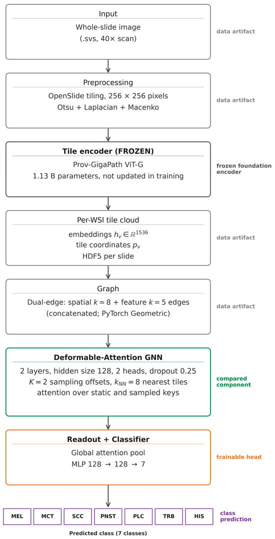
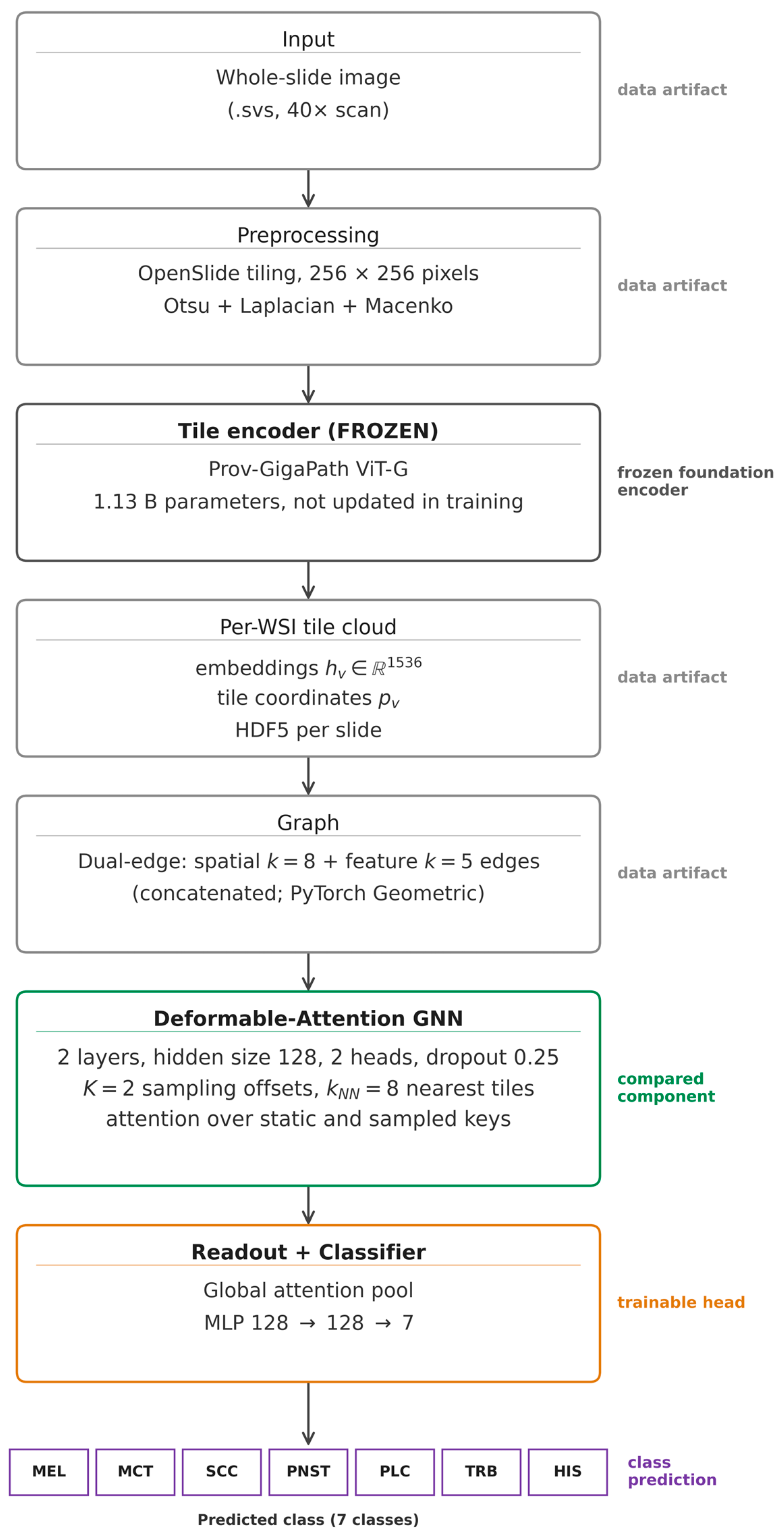
Each whole-slide image went through a three-stage pipeline (Figure 1, top half).

Figure 1. GigaPath-DefGNN pipeline. A frozen Prov-GigaPath vision transformer (ViT-G; 1.13 B parameters) embeds 256 × 256 tiles obtained by OpenSlide tiling, tissue and blur filtering, and Macenko stain normalization. The 1536-dimensional embeddings and tile coordinates are stored per slide, a dual-edge graph (spatial k = 8 and feature k = 5 edges) is built, and a two-layer deformable graph-attention stack (hidden size 128, 2 heads, K = 2 offsets, kNN = 8) is followed by a global attention readout and an MLP classifier (128 → 128 → 7). The deformable layer is the component compared against the other aggregators; every other block is shared by all models.

Tiling. OpenSlide [27] reads the .svs file. Tissue regions were detected by Otsu thresholding on the HSV (hue–saturation–value)-converted image. Non-overlapping 256 × 256-pixel tiles were extracted at the 40× equivalent magnification and kept when the tissue ratio exceeded 0.5 and the Laplacian variance exceeded 100 (a blur filter). Tiles were color-normalized with Macenko stain normalization [28]. This 40× (0.25 μm/pixel) extraction is finer than Prov-GigaPath’s 20× (0.5 μm/pixel) pretraining resolution; the effect of this mismatch is quantified in Section 3.7, where the headline models are also repeated at 20×.

For the magnification analysis (Section 3.7), every slide was also tiled at 20× equivalent (0.5 μm/pixel), matching Prov-GigaPath’s pretraining resolution. The CATCH files contain no native 20× pyramid level, so each 20× tile was obtained by reading a 512 × 512-pixel region at level 0 on a 512-pixel grid and box-filtering it to 256 × 256 pixels, with the same tissue, blur, and Macenko steps as at 40×. The 20× grid is aligned with the 40× grid, so each 20× tile covers exactly the area of four 40× tiles. To reduce tiling time, grid cells whose tissue fraction on a ~16×-downsampled thumbnail was below 1% were skipped before reading. On 57 slides (261,228 kept tiles), this rule skipped 49.5% of the cells and no kept tile (the lowest thumbnail tissue fraction of any kept tile was 0.513), and re-tiling two slides with and without it produced byte-identical tiles. One slide (HIS_22_1, 87 tiles at 40×) yielded only 6 tissue tiles at 20×, below the minimum of 16 tiles per slide applied throughout, and was excluded from the 20× experiments only, which therefore use 349 WSIs; the 20× tile embeddings were computed with the same frozen encoder and precision as at 40×.

Feature extraction. A frozen Prov-GigaPath tile encoder (a vision transformer, ViT-G, with 1.13 B parameters, not updated during training) [2] processed each tile and produced a 1536-dimensional embedding, stored together with the tile’s top-left level-0 coordinates (x, y) in a per-slide HDF5 (hierarchical data format) file. Inference used a batch size of 256 in half-precision (fp16) mixed precision.

Graph construction. For each slide, we built a dual-edge graph by concatenating the edges of (i) a spatial k-NN graph (k = 8) and (ii) a feature k-NN graph (k = 5, cosine similarity), each symmetrized; duplicate edges are kept, giving 26 incoming edges per node on average. The graph is stored as a PyTorch Geometric object with node features, edges, per-edge attributes (inverse distance for spatial edges and cosine similarity for feature edges; not used by any of the models), and tile coordinates.

For the graph-construction ablation (Section 3.6) we used the two branches of the dual-edge graph on their own—the spatial k-NN graph (k = 8) and the feature k-NN graph (k = 5), obtained by keeping only the spatial or only the feature edges of each dual-edge graph, so that the neighbors are identical—and, as an additional variant, a feature-similarity graph that links tiles whose embeddings have a cosine similarity of at least 0.8, keeping at most 8 edges per node (thresholded; it leaves some tiles without edges).

End-to-end preprocessing took about 100 active GPU-hours on a single NVIDIA RTX 3090 (24 GiB VRAM): tiling ~30 GPU-h, feature extraction ~55 GPU-h, and graph construction ~15 GPU-h.

2.4. GigaPath-DefGNN—Coordinate-Aware Deformable Graph Attention

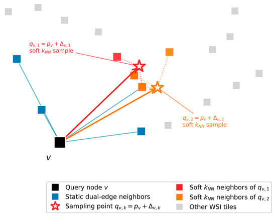
GigaPath-DefGNN (Figure 1, bottom half; Figure 2 for the deformable-attention layer on its own) has three parts: (i) two stacked deformable-attention layers operating on the dual-edge graph and the frozen Prov-GigaPath features, (ii) a Global Attention Readout that pools the per-node embeddings into a slide-level vector through a learned per-node attention gate, and (iii) a two-layer MLP (multilayer perceptron) classifier (128 → 128 → 7, dropout 0.25). Total trainable parameters are about 1.32 M, against ~445 K for the standard GAT baseline at matched hidden/heads/layers; the deformable mechanism roughly triples the aggregator-head parameter count, an overhead of ~875 K. That overhead is dominated not by the OffsetMLP (only ~6.7 K) but by each layer’s independent query, static-key/value, and sampled-key/value projections together with the residual skip projection—each mapping from the 1536-dimensional input in the first layer. Even so, the whole trainable head is ~0.1% of the frozen 1.13 B-parameter Prov-GigaPath encoder. Per-component counts are released in results/param_counts.json (regenerable with scripts/16_param_counts.py).

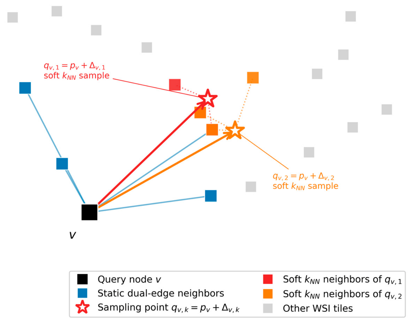
Figure 2. Deformable-attention layer schematic. The query node v (black) sits within its static dual-edge neighborhood (blue). The OffsetMLP predicts K = 2 sampling offsets (red and orange arrows) from (hv, pv) with pv = (xv, yv) to query positions qv,k = pv + Δv,k (open stars). Soft k-nearest-neighbor sampling at each offset pulls in kNN nearest tile features (red and orange squares). Attention is computed jointly over the union of static neighbors and the K sampled positions. Schematic, not to scale: the learned first-layer offsets are much longer than drawn (median 51 tile spacings; Section 2.4.2).

2.4.1. Deformable-Attention Layer

For each node v with embedding h_v and tile coordinate p_v = (x_v, y_v), the layer worked as follows:

$$h_v \in {\mathbb{R}}^{d_{in}}, p_v = \left(x_v, y_v\right) \in {\mathbb{R}}^2$$

1. Offset prediction. A small MLP predicted K = 2 sampling offsets per node:

$${\Delta }_v = \mathit{OffsetMLP}\left(h_v, p_v\right) \in {\mathbb{R}}^{K\times 2}$$

We set K = 2 to fit the densest CATCH WSIs (~94,000 tiles) on a 24 GiB GPU (Section 3.5). The OffsetMLP was initialized with a small output scale. The configuration also specifies an L2 penalty on the offsets, but during the revision we found that this term was never added to the training loss: no offset penalty was applied in any run (Section 3.5). The learned offsets are large (Section 2.4.2).

2. Soft k-nearest-neighbor sampling. For each query coordinate q_v,k = p_v + Δ_v,k:

$$q_{v,k} = p_v + {\Delta }_{v,k}$$

the layer found the k_NN = 8 tile-coordinate nearest neighbors {u₁, …, u_kNN} via torch_cluster.knn (no full N × N distance matrix was materialized), then interpolated features as:

$$s_{v,k} = {\sum }_i {\mathit{softmax}\left(-{\displaystyle \frac{{\Vert q_{v,k} - p_{u_i}\Vert }^2}{T}}\right)}_i · h_{u_i}$$

with temperature T = 1. Queries were processed in chunks to bound peak memory independent of WSI size (1024 queries per chunk in the original runs and 16,384 in the runs added in this revision; the chunk size changes runtime only, not the selected neighbors).

3. Q/K/V projections. Two separate K/V projections—one for the static path, one for the deformable-sampled path—shared a single query projection (static path):

$$q_v = W_Q{h}_v, k_v^{\left(s\right)} = W_K^{\left(s\right)}{h}_v, v_v^{\left(s\right)} = W_V^{\left(s\right)}{h}_v$$

and the deformable-sampled path:

$$k_{v,k}^{\left(d\right)} = W_K^{\left(d\right)}{s}_{v,k}, v_{v,k}^{\left(d\right)} = W_V^{\left(d\right)}{s}_{v,k}$$

4. Vectorized attention over static ∪ deformable. For each destination node v, the attention scores were the scaled dot-products

$$e_{v,u}={\displaystyle \frac{q_v · k_u}{\sqrt{d_{head}}}}$$

over the union of (i) edges from the static dual-edge graph incoming to v and (ii) K virtual self-edges with keys k^(d)_v,1,…,K, where d_head is the per-head dimension. A fused scatter-softmax (PyTorch Geometric’s softmax) was applied to these scores across the union,

$${\alpha }_{v,u}={softmax}_u\left(e_{v,u}\right)$$

and a weighted-sum scatter produced the per-node output:

$${h_v}^{\prime } = W_O {\sum }_{u \in static \cup K_d} {\alpha }_{v,u} · v_u$$

5. Residual + LayerNorm.

$${h_v}^{″}=\mathit{LayerNorm}\left({h_v}^{\prime }+\mathit{skip}\left(h_v\right)\right)$$

The training-time forward pass was wrapped in torch.utils.checkpoint.checkpoint, so the sampling-pass intermediates were recomputed during backward rather than kept in memory; without this, the accumulated activations exhausted memory at about 22 GiB on the largest CATCH WSI.

2.4.2. Relation to Existing Aggregators

To make the difference from existing aggregators explicit, we write each model in one notation. Let h_v be the frozen embedding of tile v, p_v ∈ [0, 1]² its tile coordinate after per-slide min–max normalization, N(v) its in-neighbors in the static dual-edge graph (which has no self-loops), and z the slide vector passed to the classifier. The models differ in (i) the support set over which a node or the slide attends, (ii) the scoring function, and (iii) whether coordinates enter the scoring or only the graph construction.

MIL pooling (ABMIL, CLAM, ACMIL) forms z = Σ_v a_v φ(h_v) with gated-attention weights a_v = softmax_v(w^T[tanh(Vφ(h_v)) ⊙ σ(Uφ(h_v))]) over all tiles, so the support set is the whole slide and coordinates play no role; CLAM-MB and ACMIL use several such branches. DSMIL scores tiles by their similarity to a critical instance. Our TransMIL applies full softmax self-attention to all tiles (Section 2.5). Static graph attention (GAT) computes h′_v = Σ_{u ∈ N(v) ∪ {v}} α_vu W h_u with α_vu = softmax_u(LeakyReLU(a^T[W h_v ‖ W h_u])); coordinates enter only through the spatial edges, and GCN, GraphSAGE (graph sample-and-aggregate), and GIN replace αvu with fixed normalized, mean, or sum weights. Dynamic feature graphs (WiKG) rebuild each node’s neighborhood at every forward pass as the top-k tiles by learned embedding similarity over the whole slide, so the support is learned but chosen in embedding space.

Deformable graph attention (GigaPath-DefGNN; Section 2.4.1) adds K sampled keys W_K^(d) s_v,k to the static keys {W_K^(s) h_u: u ∈ N(v)}, where s_v,k is a softmax-distance-weighted average of the k_NN tiles nearest q_v,k = p_v + Δ_v,k, and scores all keys with a scaled dot product against W_Q h_v. Coordinates therefore enter the scoring itself, a property that no baseline shares. Three properties follow from the definition.

Property 1 (sampling is local averaging). When the squared distances from q_v,k to its k_NN nearest tiles differ by much less than T, the weights approach 1/k_NN and s_v,k becomes the mean of those tiles. Coordinates are min–max normalized per axis and per slide, so adjacent tiles lie so close together that, at T = 1 and for a query point on the tile grid, the weight of a tile three spacings away differs from that of an adjacent tile by 0.012% on the median slide and by at most 0.17% on any of the 350 slides (along the slide’s shorter axis, where the normalized spacing is largest). For query points on or near tissue, each sampled key is therefore, in effect, a local mean taken at a learned location.

Property 2 (small offsets add little). As Δ_v,k → 0, the query point coincides with p_v, and the sampled key becomes the mean of v and its nearest tiles, which largely overlap N(v) (the two neighborhoods can differ because the sampling uses per-axis normalized coordinates and the static graph pixel coordinates). The layer then adds, beyond the static graph, essentially a local mean that includes v’s own embedding; information from outside the neighborhood requires offsets comparable to, or larger than, the tile spacing.

Property 3 (not a GAT at K = 1). For any K, the layer differs from GAT in its scoring function (dot-product versus additive), its projections (separate versus shared key and value), and its static support (no self-loop). Equal validation accuracies of the K = 1 model and GAT (Section 3.5) are therefore not evidence of a functional identity.

What the learned offsets sample. We recorded the offsets of the trained models on all 350 test WSIs (one tile spacing = 256 pixels = 64 μm at 40×). In the first layer, the per-WSI median offset length was 51 tile spacings (median over WSIs; interquartile range 35–78), and on the median WSI, 14% of the query points fell outside the slide’s tile bounding box, and only 48% lay within one tile spacing of a tissue tile. In the second layer, the offsets were shorter (7.1 tile spacings; interquartile range 4.8–10.0), and on the median WSI, 82% of the query points lay within one tile spacing of a tissue tile. By Property 1, the mechanism therefore injects millimeter-scale context in the first layer—often the mean of tissue-boundary tiles near a background point—and sub-millimeter context in the second, rather than deforming the local neighborhood. It gives nodes access to context beyond the static graph that the MIL poolings already obtain through their slide-wide support.

Cost. Per layer, MIL pooling costs O(N d) for N tiles and embedding width d; static graph aggregation costs O(E d) for E edges; our TransMIL (full self-attention) and WiKG (dynamic neighbor search) cost O(N2 d); and the deformable layer costs O((E + N K kNN) d) for attention and sampling plus the k-NN search of the N K query points, which torch_cluster performs by brute force in O(N2 K) distance evaluations. Measured parameters and floating-point operations (FLOPs) are in Section 3.9.

2.5. Baselines

We compared GigaPath-DefGNN with 13 baselines that used the same frozen Prov-GigaPath features, CATCH splits, and training configuration (Section 2.2 and Section 2.6); only the aggregator differed.

MIL aggregators (eight). ABMIL [8], DSMIL [9], TransMIL [10], CLAM-SB and CLAM-MB [11] trained with the common cross-entropy objective only, CLAM-SB and CLAM-MB trained with CLAM’s instance-level clustering loss (“inst.”; top/bottom 8 instances, bag weight 0.7, subtyping setting), and ACMIL [12] (five attention branches, stochastic top-10 instance masking with ratio 0.6, and its branch and attention-diversity losses).

GNN aggregators (five). GCN [29], GraphSAGE [30], GAT [17], and GIN [31] on the dual-edge graph (Section 2.3) with hidden size 128, 2 attention heads (GAT), 2 layers, and dropout 0.25, as in GigaPath-DefGNN, and the dynamic-graph WiKG [16] (top-6 neighbors, bi-interaction aggregation).

All baselines are re-implementations that consume the tile embeddings directly. We state where they depart from the original publications. CLAM-SB without the instance loss differs from gated-attention ABMIL only in its dropout (0.25 versus 0). TransMIL is a standard two-layer Transformer encoder with a class token, without the pyramid position encoding generator (PPEG; it assumes a square tile grid) and without the Nyström approximation. DSMIL averages its instance and bag streams and is trained with the slide loss only. ACMIL and WiKG were ported from the official code, and WiKG’s neighbor search is computed in row chunks so that it fits the largest WSIs in memory (its logits match the official implementation to within 4 × 10⁻⁶).

2.6. Training Configuration

Every model in this paper was trained with the configuration in Table 2; only the aggregator—and, for ACMIL and CLAM (inst.), its auxiliary training losses—differed.

Table 2. Common training configuration of all aggregators.

Hyperparameter	Value
Optimizer	AdamW [32]; learning rate 1 × 10−4; weight decay 1 × 10−5
Scheduler	5 warm-up epochs, then cosine annealing with warm restarts [33] (restart period 95 epochs, so no restart occurred before early stopping); gradient clipping at norm 1.0
Maximum epochs	100, early stopping on validation balanced accuracy (patience 15); top-3 checkpoints retained
Batch	1 WSI per batch, gradient accumulation = 8
Loss	Cross-entropy without class weights (classes are balanced, 50 WSIs each)
Precision	fp16 mixed precision with dynamic loss scaling. The original safeguard stopped a run at the first non-finite gradient; it stopped the published GCN and GIN runs and the first ACMIL and WiKG attempts, which were re-run. Runs started after the correction stop only after 50 consecutive non-finite (scaled) gradients or a non-finite loss. Apart from the stopped published GCN and GIN runs, which are reported only for comparison, every run ended by regular early stopping (Section 3.8)
Splits + seeds	Patient-level five-fold cross-validation; seeds {42, 123, 456, 789, 1024} per fold, except the five original MIL models (seed 42 in all folds)
Hardware	Single NVIDIA RTX 3090 (24 GiB VRAM), 64 GiB RAM
Reproducibility	All random number generators seeded; the PyTorch Geometric scatter operations are non-deterministic on GPU, so repeated fp16 runs agree to within numerical tolerance rather than bit for bit

GigaPath-DefGNN uses hidden size 128, 2 attention heads, 2 layers, dropout 0.25, K = 2 sampling offsets, k_NN = 8, a one-layer OffsetMLP with 64 hidden units computed in single precision (fp32), and per-slide coordinate normalization to [0, 1]. The K = 2 choice is discussed in Section 3.5. No offset penalty was applied (Section 2.4.1).

2.7. Metrics and Statistical Methodology

The primary metric is balanced accuracy (the macro-average of per-class recall) on the pooled out-of-fold test predictions (n = 350 WSIs). Secondary metrics are macro F1 and macro one-versus-rest area under the receiver operating characteristic curve (AUROC). For comparability with the original analysis, we also report the mean ± population standard deviation of the five per-fold test balanced accuracies.

The interpretability metrics (Section 3.4), computed on the test WSIs with at least one annotated tumor tile, were (i) the intersection over union (IoU) between the top-m attended tiles (m = number of annotated tumor tiles) and the CATCH polygon tumor mask, (ii) the Pearson correlation between the continuous attention map and the binary mask, and (iii) the area under the precision–recall curve (AUC-PR) with attention as a tumor-versus-non-tumor score.

The unit of statistical analysis is the WSI. Because some patients contribute more than one WSI, 95% confidence intervals were obtained by a patient-clustered bootstrap: the 282 patients were resampled with replacement, all of a resampled patient’s WSIs were kept together, and 10,000 resamples were drawn [34]. The same resamples were used for all models, so intervals for differences are paired. GigaPath-DefGNN was compared with each baseline by the exact McNemar test on per-WSI correctness [35], with Holm correction across the baselines [36]; per-class comparisons applied the same test to the WSIs of each class. Under rule (iii), the reference is the re-run of the GigaPath-DefGNN configuration (Section 2.2). Comparisons outside these families—the graph-construction variants, the GIN diagnostic variants, and pairs chosen after inspecting the results—are reported with unadjusted p-values and labeled exploratory. The 20× models were compared with their 40× counterparts on the WSIs available at both magnifications, with Holm correction over the two model pairs. Paired attention metrics were compared with the Wilcoxon signed-rank test [37]. The validation ablations of Section 3.5 use fold-level paired t-tests and Cohen’s effect size

$$d_z={\displaystyle \frac{\mathit{mean}\left(\Delta \right)}{\mathit{std}\left(\Delta \right)}}$$

(Cohen’s d_z); with five folds (df = 4), the paired t-test has a power of about 0.14 for d_z = 0.5 at α = 0.05 (two-sided), so a non-significant fold-level result carries little evidential weight in either direction. Non-significant differences are reported as the absence of detectable evidence, not as equivalence.

2.8. Software and Reproducibility

The implementation uses PyTorch 2.10, PyTorch Geometric 2.7, torch_cluster 1.6.3, PyTorch Lightning 2.6, timm 1.0.26, scikit-learn, and SciPy. The revision analyzes are regenerated by scripts/18_test_eval.py (held-out inference), 19_test_stats.py (statistics), 20_complexity.py (parameters and FLOPs), 21_offset_stats.py (learned offsets), 22_magnification_features.py (20× versus 40× features), 24_revision_figures.py (Figure 3 and Figure 4), 06_extract_attention_maps.py (attention–annotation analysis and Figure 5), 23_gin_loss_curves.py (Figure 6), and 25_extract_feature_knn_graphs.py (feature k-NN graphs of Section 3.6). All code, configurations, locked splits, checkpoints, and per-WSI predictions will be made publicly available at https://github.com/cowrkwithu/GigaPath-DefGNN under the MIT license (accessed on 10 May 2026).

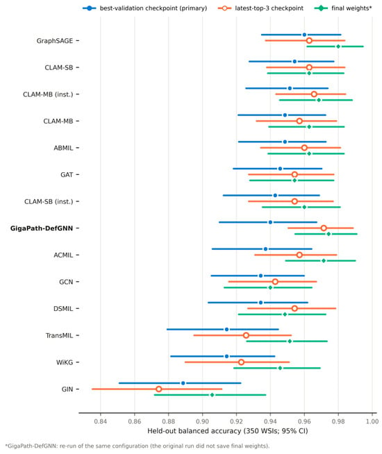
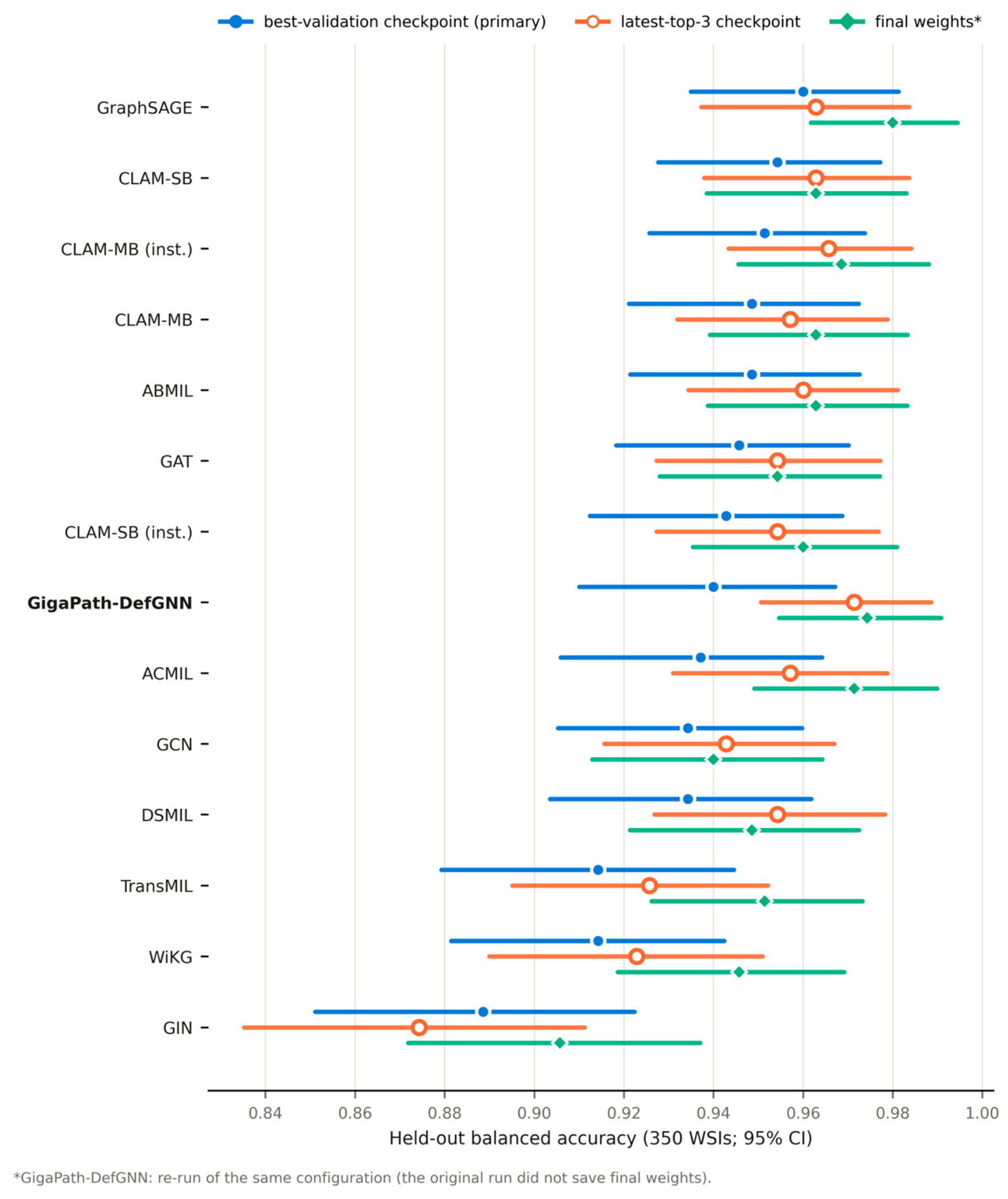
Figure 3. Held-out balanced accuracy of every evaluated aggregator (pooled out-of-fold predictions, 350 WSIs) with patient-clustered bootstrap 95% confidence intervals, under the best-validation (filled circle), latest-top-3 (open circle), and final-weights (diamond) checkpoint rules. The final-weights marker of GigaPath-DefGNN is a rerun of the same configuration, because the original run did not save its final weights (Section 3.10).

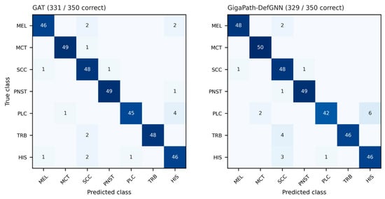
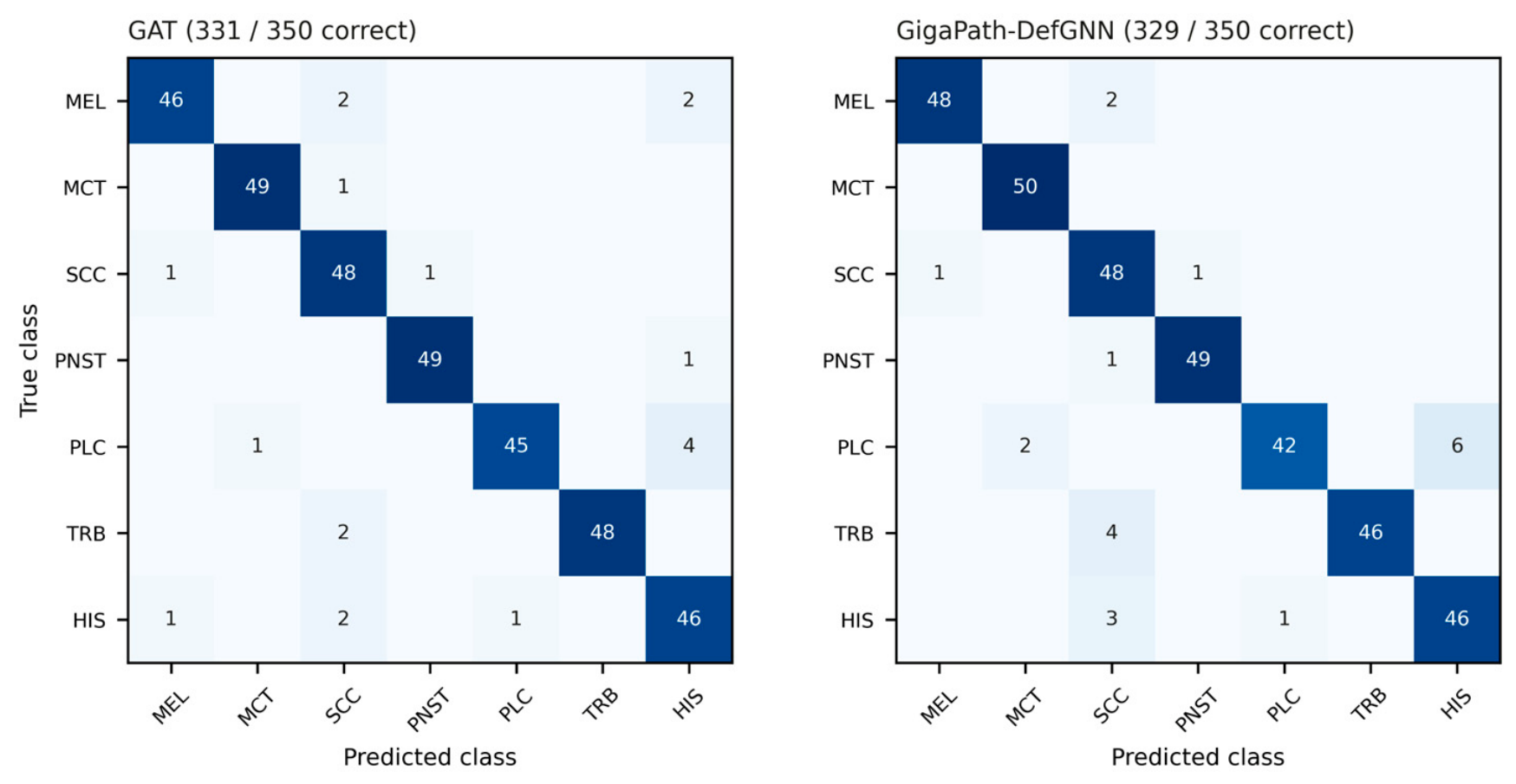
Figure 4. Pooled held-out confusion matrices (350 WSIs; best-validation checkpoints). (Left): GAT. (Right): GigaPath-DefGNN. Rows: true class; columns: predicted class.

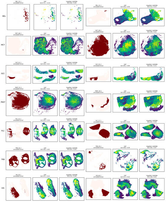
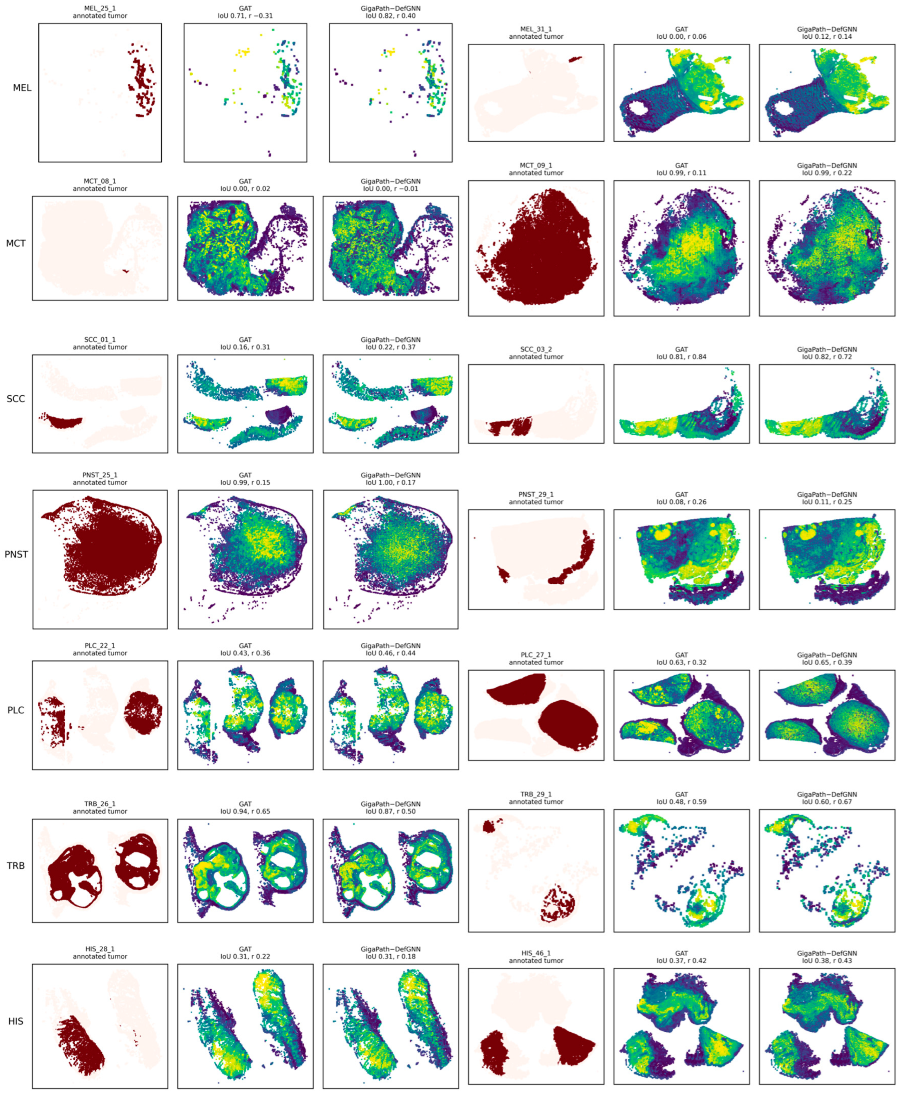
Figure 5. Attention–annotation overlays for 14 test WSIs, two per class, drawn at random (seed 0) from the WSIs with at least 20 tiles mapped to annotated tumor polygons; the selection does not depend on either model. For each WSI: annotated tumor (dark red), GAT readout attention, and GigaPath-DefGNN readout attention (within-slide percentile rank; yellow = highest), with per-WSI IoU and Pearson r. On several slides, the annotated region covers only part of the tissue while both models attend more broadly; the polygons alone cannot show whether the unannotated tissue is non-neoplastic or unannotated.

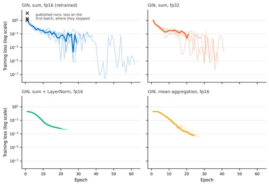
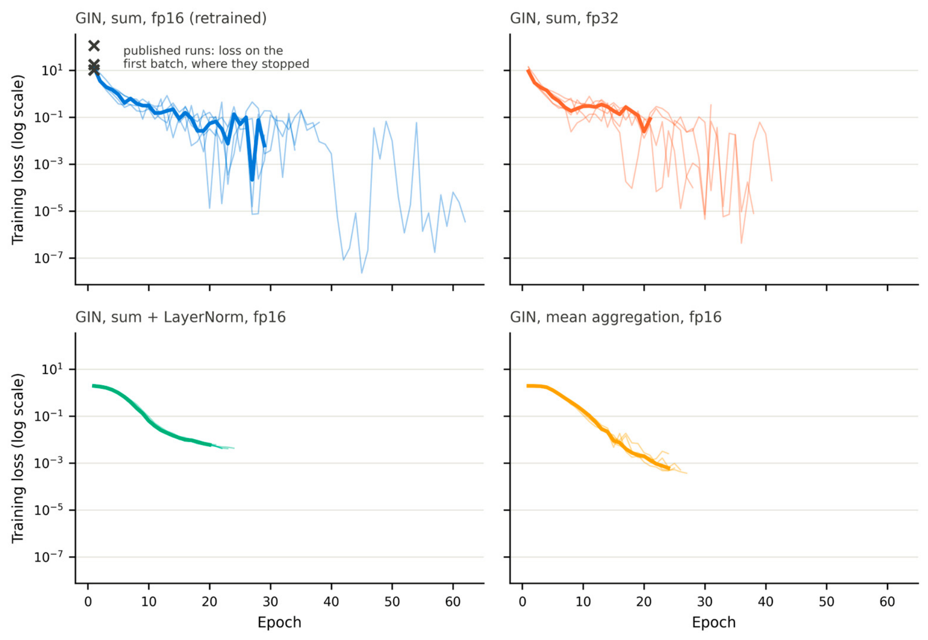
Figure 6. Per-epoch training loss (log scale) of GIN variants retrained with the corrected safeguard: sum aggregation in half precision (fp16; the published configuration) and in single precision (fp32), sum aggregation with LayerNorm, and mean aggregation. Thin lines: folds; thick line: median over folds. Crosses: training loss of the published GIN runs on their first batch, at which they were stopped.

3. Results

3.1. Held-Out Test Performance

Table 3 lists the pooled out-of-fold test performance of GigaPath-DefGNN and the baselines (all 14 aggregators) under the primary best-validation rule.

Table 3. Held-out test performance on all 350 WSIs (pooled out-of-fold predictions; best-validation checkpoints), ordered by balanced accuracy. CI: patient-clustered bootstrap 95% confidence interval. SD: population standard deviation over the five folds. Δ: GigaPath-DefGNN minus baseline, with paired bootstrap 95% CI. b/c: WSIs classified correctly only by GigaPath-DefGNN/only by the baseline. p: exact McNemar test, raw and Holm-adjusted.

Model	Balanced Accuracy [95% CI]	Fold Mean ± SD	Macro F1	Macro AUROC	Δ [95% CI]	b/c	p (Holm)
GraphSAGE	0.960 [0.935, 0.981]	0.964 ± 0.033	0.960	0.998	−0.020 [−0.042, +0.002]	5/12	0.14 (1.00)
CLAM-SB	0.954 [0.928, 0.977]	0.957 ± 0.032	0.955	0.996	−0.014 [−0.037, +0.008]	6/11	0.33 (1.00)
CLAM-MB (inst.)	0.951 [0.926, 0.974]	0.952 ± 0.032	0.952	0.995	−0.011 [−0.038, +0.015]	8/12	0.50 (1.00)
CLAM-MB	0.949 [0.921, 0.972]	0.949 ± 0.029	0.949	0.993	−0.009 [−0.031, +0.013]	5/8	0.58 (1.00)
ABMIL	0.949 [0.921, 0.973]	0.952 ± 0.033	0.949	0.995	−0.009 [−0.031, +0.014]	7/10	0.63 (1.00)
GAT	0.946 [0.918, 0.970]	0.946 ± 0.036	0.946	0.995	−0.006 [−0.027, +0.016]	6/8	0.79 (1.00)
CLAM-SB (inst.)	0.943 [0.912, 0.969]	0.944 ± 0.029	0.944	0.995	−0.003 [−0.026, +0.021]	8/9	1.00 (1.00)
GigaPath-DefGNN	0.940 [0.910, 0.967]	0.942 ± 0.036	0.940	0.997	—	—	—
ACMIL	0.937 [0.906, 0.964]	0.936 ± 0.056	0.938	0.995	+0.003 [−0.022, +0.030]	10/9	1.00 (1.00)
GCN	0.934 [0.905, 0.960]	0.935 ± 0.022	0.934	0.996	+0.006 [−0.022, +0.035]	14/12	0.85 (1.00)
DSMIL	0.934 [0.904, 0.962]	0.936 ± 0.013	0.935	0.993	+0.006 [−0.023, +0.036]	13/11	0.84 (1.00)
TransMIL	0.914 [0.879, 0.945]	0.915 ± 0.061	0.916	0.993	+0.026 [−0.006, +0.060]	20/11	0.15 (1.00)
WiKG	0.914 [0.881, 0.942]	0.916 ± 0.032	0.915	0.991	+0.026 [−0.0002, +0.054]	16/7	0.09 (1.00)
GIN	0.889 [0.851, 0.922]	0.894 ± 0.041	0.890	0.967	+0.051 [+0.011, +0.094]	32/14	0.01 (0.15)

The aggregators span a held-out balanced accuracy of 0.889–0.960, and their bootstrap intervals overlap widely, except that the interval of the retrained GIN lies entirely below those of GraphSAGE, CLAM-SB and CLAM-MB (inst.). GigaPath-DefGNN reached 0.940 [0.910, 0.967] and ranked eighth of 14. No pairwise difference between GigaPath-DefGNN and a baseline was significant (smallest Holm-adjusted p = 0.148), and every paired bootstrap interval for the difference included zero except that against GIN (Δ +0.051 [+0.011, +0.094]), which did not survive Holm correction. Macro AUROC ranged from 0.967 to 0.998 across the models, so the models differ more in their decision thresholds than in how they rank the slides.

The GCN and GIN rows are from runs retrained with the corrected training safeguard (Section 3.8). The initial runs had been stopped after 8–10 epochs (GCN) and at the first training batch, before any parameter update (GIN), and reached 0.914 and 0.154; the retrained GCN reaches 0.934 and the retrained GIN 0.889; the remaining gap of GIN reflects the scale of its unnormalized sum aggregation and disappears with a LayerNorm (Section 3.8). Under matched features, splits, and training budget, the held-out data therefore do not separate coordinate-aware deformable attention from the static-graph, dynamic-graph, and MIL aggregators.

3.2. Checkpoint Selection and Validation Optimism

Table 4 contrasts validation and held-out balanced accuracy under the three checkpoint rules.

Table 4. Validation versus held-out balanced accuracy by checkpoint rule. Validation: mean of the five per-fold validation values (the validation sets differ between folds). Test: balanced accuracy of the pooled out-of-fold predictions (350 WSIs), as in Table 3. Gap = validation − test under the best-validation rule. * The original GigaPath-DefGNN runs did not save their final weights; the rule-(iii) value is that of the re-run of the same configuration (Section 3.10).

Model	Validation (Best)	Test (Best)	Gap	Test (Latest Top-3)	Test (Final)
GraphSAGE	0.983	0.960	+0.023	0.963	0.980
CLAM-SB	0.988	0.954	+0.034	0.963	0.963
CLAM-MB (inst.)	0.976	0.951	+0.025	0.966	0.969
CLAM-MB	0.960	0.949	+0.012	0.957	0.963
ABMIL	0.988	0.949	+0.040	0.960	0.963
GAT	0.984	0.946	+0.038	0.954	0.954
CLAM-SB (inst.)	0.988	0.943	+0.045	0.954	0.960
GigaPath-DefGNN	0.988	0.940	+0.048	0.971	0.974 *
ACMIL	0.980	0.937	+0.043	0.957	0.971
GCN	0.977	0.934	+0.043	0.943	0.940
DSMIL	0.988	0.934	+0.054	0.954	0.949
TransMIL	0.971	0.914	+0.057	0.926	0.951
WiKG	0.964	0.914	+0.050	0.923	0.946
GIN	0.954	0.889	+0.066	0.874	0.906

Validation performance overstated held-out performance for every model: under the best-validation rule the gap was +0.012 to +0.066 (median +0.043; GIN largest, GigaPath-DefGNN +0.048). Several models reach the validation ceiling while differing on the test partitions, so a 37–39-WSI validation set cannot rank models whose true differences are of this size. The checkpoint rule moved pooled test balanced accuracy by amounts comparable to the differences between aggregators: replacing the best-validation checkpoint by the final weights changed it by +0.006 to +0.037 across the baselines (TransMIL +0.037, ACMIL +0.034, WiKG +0.031; median +0.017), whereas two aggregators differed by a median of 0.014 and the aggregators other than the retrained GIN spanned 0.046 in Table 3 (0.914–0.960). The best-validation checkpoints come from early epochs, where the validation metric first saturates.

The ranking itself depends on the rule (Figure 3). Under the latest-top-3 rule, GigaPath-DefGNN had the highest pooled test balanced accuracy (pooled over 350 WSIs: 0.971 [0.951, 0.989]), moving from eighth to first place; it exceeded GIN, TransMIL, and WiKG after Holm correction but no other baseline. With final weights, represented by the re-run of the same configuration (Section 3.10), it reached 0.974 [0.955, 0.991] and ranked second behind GraphSAGE (0.980 [0.962, 0.994]; Δ +0.006 for GraphSAGE, Holm-adjusted p = 1.00), and exceeded GIN after Holm correction but no other baseline. Under none of the three rules did GigaPath-DefGNN significantly outperform a baseline other than these three lowest-ranked ones (GIN, TransMIL and WiKG), and no baseline significantly outperformed it under any rule. With the best-validation rule applied to every model, the validation advantage reported for GigaPath-DefGNN in the original analysis also disappears: ABMIL, DSMIL, CLAM-SB, and CLAM-SB (inst.) all reach the same validation value as GigaPath-DefGNN (0.988) (Table 4).

3.3. Per-Class Performance on Held-Out Data

Table 5 lists per-class F1 on the pooled test predictions (50 WSIs per class; best-validation rule).

Table 5. Per-class F1 on all 350 test WSIs (pooled out-of-fold predictions; best-validation checkpoints).

Model	MEL	MCT	SCC	PNST	PLC	TRB	HIS
GraphSAGE	0.948	0.990	0.935	1.000	0.941	0.980	0.928
CLAM-SB	0.948	0.980	0.935	0.990	0.939	0.969	0.923
CLAM-MB (inst.)	0.948	0.970	0.951	0.990	0.918	0.980	0.906
CLAM-MB	0.959	1.000	0.925	0.980	0.926	0.969	0.885
ABMIL	0.948	0.970	0.926	0.990	0.938	0.969	0.904
GAT	0.939	0.980	0.914	0.980	0.938	0.980	0.893
CLAM-SB (inst.)	0.938	0.980	0.917	0.990	0.928	0.959	0.893
GigaPath-DefGNN	0.970	0.980	0.889	0.980	0.903	0.958	0.902
ACMIL	0.938	0.980	0.925	0.980	0.900	0.969	0.876
GCN	0.882	0.960	0.889	0.980	0.940	0.980	0.911
DSMIL	0.911	0.980	0.941	0.980	0.900	0.980	0.851
TransMIL	0.915	0.949	0.895	0.980	0.882	0.970	0.818
WiKG	0.917	0.970	0.865	0.990	0.854	0.959	0.851
GIN	0.889	0.891	0.889	0.949	0.878	0.928	0.804

Across models, F1 was highest for PNST, MCT, and trichoblastoma (means over models 0.968–0.983) and lowest for histiocytoma (mean 0.882, range 0.804–0.928). Plasmacytoma predicted as histiocytoma—a confusion between two round-cell neoplasms—was the most frequent error of GigaPath-DefGNN (6 of 21 errors) and of GAT (4 of 19), and no aggregator resolved it.

GigaPath-DefGNN had the highest melanoma F1 of all models (0.970) and ranked between third and thirteenth of 14 on the other classes. Its lower squamous cell carcinoma F1 (0.889) did not come from missed carcinomas (48 of 50 SCC slides were recognized) but from 10 slides of other classes predicted as SCC. Per-class exact McNemar tests between GigaPath-DefGNN and each baseline found no difference that survived correction for the number of class-by-baseline comparisons, and the direction of the per-class differences was not stable across checkpoint rules. These data do not support the class-conditional reading of the original analysis (a lift on focal tumors with no change on the diffuse SCC class), which rested on validation sets with 3–8 WSIs per class; we found no evidence of systematic harm to diffuse or irregular tumors either.

Pooled test confusion matrices for GAT and GigaPath-DefGNN are shown in Figure 4.

3.4. Attention–Annotation Alignment on Held-Out Data

We compared the global-attention readout weights of GAT and GigaPath-DefGNN—the readout module is identical in the two models—with the CATCH polygon tumor annotations on the test WSIs, using the metrics of Section 2.7 and the best-validation checkpoints (Table 6). Of the 350 test WSIs, 275 had at least one tile mapped to an annotated tumor polygon and were analyzed; the other 75 had no mapped tumor tile (Section 4.3).

Table 6. Attention–annotation alignment on the 275 test WSIs with annotated tumor tiles (paired by WSI).

Metric	GAT	GigaPath-DefGNN	Mean Paired Δ	Paired Wilcoxon p	WSIs Where GigaPath-DefGNN Is Higher
IoU, mean (median)	0.391 (0.329)	0.381 (0.315)	−0.009	0.11	99/275
Pearson r, mean (median)	0.252 (0.224)	0.253 (0.226)	+0.001	0.90	137/275
AUC-PR, mean (median)	0.477 (0.480)	0.470 (0.474)	−0.007	0.32	138/275

The attention maps of both models were positively associated with the annotated tumor (Pearson r greater than zero, Wilcoxon signed-rank p = 2.0 × 10⁻²⁸ for GAT and 6.6 × 10⁻³¹ for GigaPath-DefGNN), so the readout concentrates on the tumor whether or not coordinates enter the attention. The two models did not differ on any metric (Table 6).

Table 7 breaks the IoU down by class.

Table 7. Per-class attention–annotation IoU on the test WSIs (mean ± sample SD; n = 275).

Class	n	GAT IoU	GigaPath-DefGNN IoU	Δ
MEL	41	0.392 ± 0.348	0.384 ± 0.333	−0.009
MCT	30	0.487 ± 0.445	0.486 ± 0.446	−0.001
SCC	44	0.310 ± 0.292	0.296 ± 0.258	−0.014
PNST	32	0.591 ± 0.450	0.592 ± 0.449	+0.001
PLC	47	0.316 ± 0.329	0.306 ± 0.324	−0.010
TRB	44	0.385 ± 0.395	0.373 ± 0.382	−0.012
HIS	37	0.335 ± 0.296	0.318 ± 0.274	−0.017

Per-class IoU differences ranged from −0.017 to +0.001. This does not reproduce the attention analysis of the original version, in which, on the validation WSIs, the median Pearson correlation rose from 0.147 (GAT) to 0.184 (GigaPath-DefGNN) and melanoma IoU rose by 0.067. That analysis compared the latest of the highest-validation GigaPath-DefGNN checkpoints (the latest-top-3 rule) with GAT’s final weights on 156 validation WSIs (127 paired); with one checkpoint rule and the larger held-out set, neither difference reappears. The interpretability gain therefore joins the accuracy gain as a validation-set effect that does not transfer to held-out data (Section 4.2).

Figure 5 is revised accordingly. The original figure showed, for each class, the two WSIs with the largest IoU gain for GigaPath-DefGNN, a selection that favors that model by construction. The revised figure shows two test WSIs per class drawn at random (fixed seed) from those with at least 20 annotated tumor tiles.

3.5. Ablation

Table 8 summarizes the ablations of the deformable layer. The K and k_NN sweeps (Table 9 and Table 10) and the offset-penalty runs (Table 11) were run in the original analysis and are validation-set results (best-validation checkpoints); they are reported for completeness and, given Section 3.2, should be read as indicative only. Configurations that exceeded the memory of a 24 GiB GPU are marked OOM (out of memory). The graph-construction ablation added in this revision is evaluated on the held-out test partitions (Section 3.6).

Table 8. Ablation dimensions explored for the deformable layer of GigaPath-DefGNN.

Dimension	Default (Headline)	Sweep Range	Status
K (sampling offsets)	2	{1, 2} (feasible); {4, 8} OOM	Completed—Table 9
kNN (k-NN neighbors per query)	8	{4, 8} (feasible); {16} OOM	Completed—Table 10
Offset L2 penalty weight	— (not implemented)	{0, 1 × 10−4}	Not applied (see Table 11)
Graph construction	dual-edge	{spatial k-NN, feature k-NN, feature similarity, dual-edge}	Section 3.6 (test)

Table 9. K ablation (validation balanced accuracy, five-fold patient-level cross-validation). K = 1 and K = 2 use the same OffsetMLP, k_NN = 8, optimizer, and locked splits; only the number of sampled offsets per node differs. Regenerated by scripts/13_k_ablation_table.py. Validation-set results (original analysis).

K	Per-Fold Val_Bacc	Mean	Std	Δ vs. K = 1	Cohen’s dz	Paired-t p
1	[1.0000, 1.0000, 0.9762, 0.9796, 0.9405]	0.9793	0.0218	(ref)	—	—
2	[1.0000, 1.0000, 0.9762, 1.0000, 0.9643]	0.9881	0.0151	+0.0088	0.73	0.179

Table 10. (validation balanced accuracy, five-fold patient-level cross-validation). k_NN = 4 and k_NN = 8 use the same OffsetMLP, K = 2, optimizer, and locked splits; only the number of sampled neighbors differs. Regenerated by scripts/14_knn_ablation_table.py. Validation-set results (original analysis).

kNN	Per-Fold Val_Bacc	Mean	Std	Δ vs. kNN = 8	Cohen’s dz	Paired-t p
4	[1.0000, 1.0000, 1.0000, 1.0000, 0.9643]	0.9929	0.0143	+0.0048	0.45	0.374
8 (headline)	[1.0000, 1.0000, 0.9762, 1.0000, 0.9643]	0.9881	0.0151	(ref)	—	—
16	OOM at the backward step (~1 000 MiB short on a 24 GiB RTX 3090; 22.29 GiB resident before failure)	—	—	—	—	—

Table 11. Two runs of the same GigaPath-DefGNN configuration that were labeled as offset-penalty settings (p = 0 and p = 1 × 10⁻⁴) in the original analysis. The penalty was never added to the training loss, so the rows are repeat runs; the 1 × 10⁻³ row is a single-epoch smoke test. Validation-set results (original analysis).

Penalty	Per-Fold Val_Bacc	Mean	Std	Δ vs. p = 1 × 10−4	Cohen’s dz	Paired-t p
0	[1.0000, 1.0000, 0.9762, 1.0000, 0.9643]	0.9881	0.0151	+0.0000	—	— (identical runs)
1 × 10−4 (default)	[1.0000, 1.0000, 0.9762, 1.0000, 0.9643]	0.9881	0.0151	(ref)	—	—
1 × 10−3	Single-epoch smoke test on fold 0 only(val_bac 0.6466)	—	—	—	—	—

At K = 1, the per-fold validation accuracies of GigaPath-DefGNN equal those of GAT. This is a coincidence of a coarse metric rather than a functional identity (Section 2.4.2, Property 3), and the two values also came from different checkpoint rules (best-validation versus final weights); we therefore no longer interpret K = 1 as a mechanism-off control.

Within the GPU-feasible range, K = 2 was not worse than K = 1 on any fold and was better on two folds. The mean difference (+0.009) is within the fold-to-fold variation, and the held-out results of Section 3.1 show no advantage of the K = 2 model over the baselines.

Both the default of Fu et al. [18] (K = 4) and K = 8 exceeded the memory budget at the attention-scatter step on the largest CATCH WSIs, so larger K could not be tested.

k_NN = 4 and k_NN = 8 differed on one fold only (mean +0.005 for k_NN = 4, paired-t p = 0.37); the headline configuration keeps k_NN = 8.

The offset-penalty sweep of the original analysis (Table 11) did not test a penalty: the penalty term was never added to the training loss, so its two rows are repeat runs of one configuration. Their identical validation results show only that this configuration reproduced on the validation metric.

Taken together, the validation-set ablations show that the model is insensitive to the offset count within the feasible range and to the neighborhood size. They do not show that the coordinate-aware mechanism improves on a static graph, which the held-out evaluation (Section 3.1 and Section 3.4) does not support either.

3.6. Graph-Construction Ablation

To test whether the dual-edge graph is necessary, GAT and GigaPath-DefGNN were trained on the spatial k-NN graph alone, the feature k-NN graph alone, the thresholded feature-similarity graph (Section 2.3), and the dual-edge graph, with everything else unchanged, and evaluated on the held-out test partitions (Table 12).

Table 12. Graph-construction ablation on the 350 held-out WSIs: balanced accuracy with patient-clustered bootstrap 95% CI, macro F1, and macro AUROC under the best-validation rule, and balanced accuracy (BA) under the latest-top-3 and final-weights rules. * Final weights of the re-run of the dual-edge GigaPath-DefGNN configuration (Section 3.10).

Model	Graph	Balanced Accuracy [95% CI]	Macro F1	Macro AUROC	BA, Latest Top-3	BA, Final
GAT	Spatial k-NN (k = 8)	0.954 [0.929, 0.977]	0.955	0.995	0.957	0.954
GAT	Feature k-NN (k = 5)	0.937 [0.907, 0.964]	0.938	0.994	0.954	0.957
GAT	Feature similarity (cos ≥ 0.8)	0.949 [0.922, 0.973]	0.949	0.995	0.949	0.960
GAT	Dual-edge (spatial + feature)	0.946 [0.918, 0.970]	0.946	0.995	0.954	0.954
GigaPath-DefGNN	Spatial k-NN (k = 8)	0.949 [0.923, 0.971]	0.949	0.997	0.966	0.974
GigaPath-DefGNN	Feature k-NN (k = 5)	0.971 [0.951, 0.988]	0.971	0.996	0.980	0.980
GigaPath-DefGNN	Feature similarity (cos ≥ 0.8)	0.923 [0.891, 0.952]	0.923	0.995	0.966	0.969
GigaPath-DefGNN	Dual-edge (spatial + feature)	0.940 [0.910, 0.967]	0.940	0.997	0.971	0.974 *

For GAT, no graph was consistently better: under the primary rule, balanced accuracy ranged from 0.937 to 0.954 across the four graphs, and the dual-edge graph (0.946) lay inside this range. For GigaPath-DefGNN, the spatial-only (0.949) and dual-edge (0.940) graphs were close; the thresholded feature-similarity graph was lowest (0.923), and the feature k-NN graph gave the highest value under all three rules (0.971, 0.980, and 0.980; fold SD ≤ 0.012). Macro F1 followed balanced accuracy for every variant (largest difference 0.001), and macro AUROC was 0.994–0.997 across the eight variants, so the other metrics do not change this picture.

We report the feature k-NN result as exploratory. It was selected after inspecting four graphs under three rules; it is not corrected for this multiplicity, and it did not transfer to GAT, which was lowest on the same graph (0.937). Against the dual-edge GigaPath-DefGNN the feature k-NN variant was correct on 12 WSIs where the dual-edge model was wrong and wrong on 1 where it was right (unadjusted exact McNemar p = 0.003), but against the strongest baselines the difference was not significant (GraphSAGE: 9/5, p = 0.42; CLAM-SB: 10/4, p = 0.18); against all 13 baselines (Holm correction over the baselines, not over the variants inspected) it exceeded only GIN, TransMIL and WiKG. Neither single branch differed significantly from the dual-edge graph for either model under the primary rule, except for this exploratory feature k-NN variant of GigaPath-DefGNN (spatial k-NN versus dual-edge, unadjusted exact McNemar p = 0.25 for GAT and 0.58 for GigaPath-DefGNN; feature k-NN versus dual-edge, p = 0.38 for GAT). The dual-edge graph is therefore not necessary for either model, and whether a feature-only neighborhood combined with coordinate-aware sampling is genuinely better would require a pre-specified test on an independent cohort. The headline configuration is unchanged.

3.7. Tile Magnification: 20× Versus 40×

Prov-GigaPath was pretrained on 20× tiles, whereas our main analysis used 40× tiles. To quantify the effect, we compared, for every WSI, each 20× tile embedding with the mean embedding of the kept 40× tiles (one to four) in the same 512 × 512-pixel region. The cosine similarity of these pairs is compared with three references: a random other region of the same slide, two 40× tiles of the same region, and one 40× tile against the mean of the other 40× tiles of its region. We also computed the linear centered kernel alignment (CKA) between the two sets of embeddings [38], the fraction of 20× tiles whose most similar 40× region is their own, and whether slide-level embeddings transfer across magnifications with a logistic-regression probe over the outer folds. We also repeated the headline experiment (GAT and GigaPath-DefGNN) on 20× tiles (Table 13).

Table 13. Headline models at 20× versus 40×: held-out balanced accuracy on the 349 WSIs available at both magnifications (paired). Δ: 20× minus 40× with paired patient-clustered bootstrap 95% CI. b/c: WSIs correct only at 20×/only at 40×. p: exact McNemar test, raw and Holm-adjusted over the two model pairs. * 40× reference under the final-weights rule: re-run of the GigaPath-DefGNN configuration.

Rule	Model	20×	40×	Δ [95% CI]	b/c	p (Holm)
Best-validation	GAT	0.960	0.945	+0.014 [−0.009, +0.038]	10/5	0.30 (0.30)
Best-validation	GigaPath-DefGNN	0.965	0.940	+0.026 [+0.003, +0.050]	12/3	0.04 (0.07)
Latest top-3	GAT	0.963	0.954	+0.009 [−0.008, +0.026]	6/3	0.51 (1.00)
Latest top-3	GigaPath-DefGNN	0.980	0.971	+0.009 [−0.008, +0.026]	6/3	0.51 (1.00)
Final	GAT	0.963	0.954	+0.009 [−0.011, +0.029]	8/5	0.58 (1.00)
Final	GigaPath-DefGNN	0.980	0.974 *	+0.006 [−0.008, +0.019]	4/2	0.69 (1.00)

The representations differ substantially between magnifications (349 WSIs; medians over slides of per-slide medians). A 20× embedding and the mean 40× embedding of the same region had a cosine similarity of 0.554 (interquartile range 0.486–0.613), against 0.309 for a random other region, 0.743 for two 40× tiles of the same region, and 0.803 for a 40× tile against the mean of the other 40× tiles of its region. The linear CKA between the two embedding sets was 0.875, only 19.6% of the 20× tiles retrieved their own region among the 40× regions of the slide, and 20× embeddings had a slightly larger norm (ratio 1.09). The magnification change thus preserves the global geometry of the embedding space but moves individual tiles far more than the variation among 40× tiles of one region. Slide-level embeddings did not transfer across magnifications: a probe trained and tested at 40× reached 0.937 balanced accuracy and one trained and tested at 20× 0.960, but training at one magnification and testing at the other gave 0.862 (40× → 20×) and 0.851 (20× → 40×).

Despite this shift, the headline models were not worse at 20×. In all six comparisons of Table 13, the 20× model scored at least as high as its 40× counterpart (Δ +0.006 to +0.026), but none of the differences survived Holm correction (smallest adjusted p = 0.07; for GigaPath-DefGNN under the primary rule Δ +0.026 [+0.003, +0.050], unadjusted p = 0.04). Per class (Table 14), the 20× models had a higher F1 for squamous cell carcinoma, plasmacytoma, and histiocytoma in all six comparisons (ΔF1 +0.001 to +0.063); these three classes were involved, as true or predicted class, in every error of GAT (19 of 19) and GigaPath-DefGNN (21 of 21) at 40× under the primary rule (Section 3.3). Mast cell tumor F1 was lower at 20× in five of the six comparisons (by 0.010–0.020 in four of them and by less than 0.001 in one) and higher in one (+0.010), and the other classes changed by −0.011 to +0.041. With 50 WSIs per class, a change of 0.02 in F1 corresponds to about one slide, so these per-class differences are descriptive. At 20×, GigaPath-DefGNN and GAT did not differ under the primary rule (6 WSIs correct only for GigaPath-DefGNN, 4 only for GAT; exact McNemar p = 0.75); with final weights, the counts were 6 and 0 (unadjusted p = 0.03; exploratory, not corrected for the three rules). Because the embeddings are magnification-specific, a model must be trained and applied at the same magnification; given that, 20× tiles, which match the encoder’s pretraining resolution, are at least as informative as 40× tiles for this task. They are also far cheaper: 7093 tiles per WSI at the median (interquartile range 3534–11,287; largest 24,777) against 26,126 at 40× for the same WSIs (3.8 times fewer tiles in total), and training GigaPath-DefGNN took a mean of 8 min per fold instead of 69 min on the same GPU (one 20× fold shared the GPU with another job). For the two headline models, the conclusions of Section 3.1 therefore do not depend on the magnification; the other aggregators were not repeated at 20×.

Table 14. Per-class F1 of the headline models at 20× versus 40× on the 349 WSIs available at both magnifications (pooled held-out predictions). Each cell: F1 at 20× and, in parentheses, the change from 40× (20× − 40×). * 40× reference under the final-weights rule: re-run of the GigaPath-DefGNN configuration.

Rule	Model	MEL	MCT	SCC	PNST	PLC	TRB	HIS
Best-validation	GAT	0.980 (+0.041)	0.990 (+0.010)	0.943 (+0.029)	1.000 (+0.020)	0.939 (+0.001)	0.969 (−0.011)	0.898 (+0.007)
Best-validation	GigaPath-DefGNN	0.980 (+0.010)	0.980 (−0.0004)	0.952 (+0.063)	0.990 (+0.010)	0.949 (+0.046)	0.980 (+0.021)	0.926 (+0.026)
Latest top-3	GAT	0.970 (+0.001)	0.980 (−0.010)	0.962 (+0.036)	0.990 (0.000)	0.939 (+0.009)	0.980 (+0.011)	0.918 (+0.009)
Latest top-3	GigaPath-DefGNN	0.990 (+0.0002)	0.980 (−0.020)	0.980 (+0.029)	1.000 (0.000)	0.960 (+0.012)	0.990 (+0.020)	0.958 (+0.018)
Final	GAT	0.980 (+0.011)	0.960 (−0.020)	0.951 (+0.008)	0.990 (0.000)	0.941 (+0.023)	0.980 (−0.010)	0.936 (+0.045)
Final	GigaPath-DefGNN *	0.990 (+0.0002)	0.980 (−0.020)	0.980 (+0.010)	1.000 (0.000)	0.960 (+0.022)	0.990 (0.000)	0.958 (+0.028)

3.8. Training Stability of GIN and GCN

In the original analysis, GIN performed at chance, and GCN trailed the other graph backbones. Both results were artifacts of a training safeguard that stopped a run at the first non-finite gradient. Under fp16 mixed precision, the gradients are inspected while still loss-scaled, and an occasional non-finite value is the normal overflow signal on which the gradient scaler skips the step and lowers the scale [39]. The safeguard had therefore stopped all five GCN runs after 8–10 epochs, and all five GIN runs at the first training batch, before any parameter update, so the published GIN result was that of an untrained network. It now stops a run only after 50 consecutive non-finite gradients or a non-finite loss. An audit of the early-stopping state stored in the final checkpoints, or of the training logs where no final checkpoint was saved, confirmed that all other runs of the original analysis, including the K and k_NN sweeps and the repeat runs labeled as a penalty sweep, had ended by regular early stopping.

GIN is prone to such overflows because its sum aggregation without normalization produces large activations on graphs with 26 edges per node on average: the first-epoch training loss of the retrained GIN was 9.5–20.1 across folds, against 1.9 with a LayerNorm inside the GIN MLP or with mean aggregation (Figure 6). With the corrected safeguard, every retrained GIN fold ended by regular early stopping (mean best-validation balanced accuracy 0.954); the fp32, LayerNorm, and mean-aggregation variants also ran to regular early stopping (0.953, 0.984, and 0.983). Held-out results of the retrained GCN and GIN are in Table 3.

The held-out results locate the remaining weakness of GIN in the scale of its sum aggregation rather than in numerical precision (balanced accuracy under the best-validation/latest-top-3/final rules): sum aggregation reached 0.889/0.874/0.906 in fp16 and 0.874/0.894/0.886 in fp32, so single precision did not help consistently, whereas adding a LayerNorm reached 0.966/0.974/0.974 and mean aggregation 0.946/0.960/0.957. With the LayerNorm, GIN was among the best models under every rule and did not differ from GraphSAGE (7/5 discordant WSIs, exact McNemar p = 0.77; exploratory). The per-epoch losses show the same picture (Figure 6): with plain sum aggregation, the training loss fluctuates over several orders of magnitude in both precisions, while the normalized variants decrease smoothly. The chance-level GIN of the original version was an untrained network, and the lower accuracy of the retrained GIN reflects an unnormalized sum over about 26 neighbors per node, not a limitation of graph isomorphism networks as such. The GIN variants are diagnostic and outside the comparison family of Table 3.

3.9. Computational Cost

Table 15 lists the trainable parameters and the inference FLOPs of every aggregator on the WSI closest to the median tile count (one of the two closest; MCT_42_1, 26,126 tiles) and on the largest WSI (TRB_10_3, 93,973 tiles). The frozen Prov-GigaPath tile encoder (1,134,953,984 parameters) is shared by all models and excluded.

Table 15. Trainable parameters and inference cost. FLOPs: dense matrix products counted by the PyTorch FLOP counter (sparse scatter aggregation and the k-NN search are not counted). Latency: fp16 inference on one RTX 3090 with no other job on the GPU, median of repeated timed runs after a warm-up; for GigaPath-DefGNN with the 16,384-query chunking of Section 2.4.1, which selects the same neighbors.

Model	Parameters	GFLOPs (Median WSI)	GFLOPs (Largest WSI)	Latency, ms (Median/Largest)
GCN	230,792	11.1	40.1	6/23
GIN	263,818	12.8	46.2	19/73
GraphSAGE	443,784	22.3	80.1	20/76
GAT	444,808	22.3	80.1	11/53
ABMIL	527,112	27.4	98.6	1/3
DSMIL	495,758	25.9	93.2	1/3
TransMIL	1,975,047	1500.7	18,455.6	25/298
CLAM-SB	527,112	27.4	98.6	1/3
CLAM-MB	528,654	27.5	98.9	2/6
CLAM-SB (inst.)	530,710	27.4	98.6	1/3
CLAM-MB (inst.)	532,252	27.5	98.9	2/6
ACMIL	470,447	24.1	86.6	1/3
WiKG	691,976	385.4	4650.8	22/260
GigaPath-DefGNN	1,319,456	90.6	325.9	207/1518

GigaPath-DefGNN needs 4.1 times the dense FLOPs of GAT on the median WSI and 3.0 times its parameters, and its k-NN sampling, which the FLOP count omits, makes it the slowest model in wall-clock time. TransMIL and WiKG have the largest FLOP counts because full self-attention and the dynamic neighbor search are quadratic in the number of tiles. Under the primary (best-validation) rule, no baseline differed significantly from GigaPath-DefGNN; under the latest-top-3 rule, it exceeded only GIN, TransMIL, and WiKG, and with final weights only GIN. The additional cost of the deformable layer therefore buys no consistent benefit on this task.

3.10. Reproducibility of the Headline Run

GigaPath-DefGNN was retrained on the dual-edge graph with the original configuration to check run-to-run reproducibility and to obtain its final weights for rule (iii) (same splits, per-fold seeds, and hyperparameters; the faster query chunking of Section 2.4.1).

The re-run reproduced the original run on held-out data without a significant difference, but not exactly. Under the best-validation rule it reached 0.937 [0.906, 0.964] against 0.940 [0.910, 0.967] for the original run (3 WSIs correct only in the original run and 2 only in the re-run; exact McNemar p = 1.00), and under the latest-top-3 rule 0.960 [0.936, 0.980] against 0.971 [0.951, 0.989] (6 and 2; p = 0.29). Its final weights reached 0.974 [0.955, 0.991]. Two runs of one configuration thus differed by up to 0.011 in balanced accuracy—the size of many of the between-model differences in Table 3. Because the GPU scatter operations are not deterministic (Table 2), this run-to-run variation is part of every result in this paper and is a further reason not to rank aggregators by point estimates on a cohort of this size.

4. Discussion

4.1. Why the Aggregators Saturate

On frozen Prov-GigaPath features, 14 aggregators that differ in support set, scoring, and use of coordinates perform within a narrow band on held-out data, and under the primary checkpoint rule none is separated from the coordinate-aware model. The most plausible reading is that the foundation embeddings already make the seven subtypes largely separable at the tile level, so the remaining errors are concentrated in histologically similar pairs—plasmacytoma and histiocytoma above all—that no pooling rule resolves. The spread between the best and the worst aggregator (0.071 balanced accuracy) is not negligible. Across all 91 pairs of aggregators under the primary rule, 3 differed after Holm correction, and all of them involve the retrained GIN (GIN versus GraphSAGE, CLAM-MB (inst.) and CLAM-SB; smallest adjusted p = 0.002), whose deficit is explained in Section 3.8; 24 pairs had an unadjusted p < 0.05. Among the other thirteen aggregators, no pair differed after correction. The saturation we describe is therefore the absence of any difference that survives correction among the aggregators other than the unnormalized GIN, not evidence that they are equivalent.

The offset measurements (Section 2.4.2) explain why coordinate-aware attention in particular adds little: its learned offsets reach millimeters into the slide and, by Property 1, bring in averaged distant context, which the MIL poolings and TransMIL already obtain through their slide-wide support. The mechanism is therefore a different route to information the other aggregators already have, not a source of new information.

This does not mean that spatial structure is irrelevant in canine cutaneous pathology; it means that, for seven-class subtyping on frozen features at this cohort size, the slide-level aggregator is not where performance is decided. Tasks that depend on spatial arrangement—grading, margin assessment, invasion—or an encoder fine-tuned on canine tissue may behave differently.

4.2. Evaluating Aggregators on Small Cohorts

Two effects in this study are as large as typical differences between aggregators. Validation estimates on 37–39-WSI folds overstated held-out accuracy for every model, and the checkpoint rule changed held-out accuracy and reordered the models (Section 3.2). The apparent advantage of GigaPath-DefGNN in our original analysis came from a validation-set comparison with mixed checkpoint rules, and its apparent interpretability gain rested on the same kind of comparison (Section 3.4); neither survived held-out evaluation with one rule.

For small veterinary cohorts we therefore recommend: (i) evaluate on held-out data, pooling out-of-fold predictions so that every slide is scored once; (ii) take the slide, not the fold, as the unit of analysis, with patient-clustered bootstrap intervals and paired tests on per-slide correctness, which gives far more resolution than a five-fold paired t-test (power about 0.14 at a medium effect); (iii) fix the checkpoint-selection rule in advance, apply it to every model, and report sensitivity to it; (iv) audit that every run ended as intended; and (v) report negative and null results with the same care as positive ones.

4.3. Limitations

The cohort is small: 350 WSIs from 282 patients, 50 per class. The held-out evaluation resolves differences of roughly two to three percentage points at best, and smaller true differences between aggregators cannot be excluded.

The validation-set ablations of Section 3.5 are subject to the same optimism as the other validation results and were not repeated on held-out data.

CATCH is predominantly single-institution. Multi-institution canine cohorts, for example in the style of the MItosis DOmain Generalization (MIDOG) challenge [24], would increase the held-out resolution and test transfer across laboratories.

The Prov-GigaPath tile encoder was frozen and not adapted to canine tissue, so the human-to-canine domain shift is left unaddressed at the representation level [5,6].

The 20× analysis used 40× scans box-filtered to 0.5 μm/pixel rather than native 20× scans, repeated only the two headline models at 20×, and excluded one slide with too little tissue at that magnification; other magnifications (for example, 10×) and other scanners were not evaluated. The embeddings were magnification-specific (Section 3.7), so the results apply to models trained and applied at one magnification.

The deformable model was restricted to K ≤ 2 offsets by GPU memory; the default K = 4 of Fu et al. [18] could not be tested.

Only one foundation model, Prov-GigaPath, was evaluated. We did not run UNI [3] or CONCH [4], so we make no claim that the results transfer to other encoders; whether the aggregators saturate in the same way on other encoders is an open question.

The CATCH annotation coverage is incomplete: on average, 36.2% of the tiles of a slide are mapped to an annotation polygon of any category, and 25.3% to a tumor polygon, and 75 WSIs have no mapped tumor tile. The attention analysis is therefore restricted to the 275 test WSIs with mapped tumor tiles, and IoU and correlation understate attention on tumor that was not annotated.

All baselines are re-implementations with a common training configuration; per-model hyperparameter tuning could change individual results. Three baselines are simplified relative to their publications (CLAM, TransMIL, and DSMIL; Section 2.5).

4.4. Future Work

Several extensions follow from the present study.

• A comparison across foundation encoders (UNI, CONCH, and canine-adapted encoders) under the same protocol.
• Multi-institution canine cohorts, for example in the style of the MIDOG challenge [24], to increase the held-out resolution.
• Tasks in which spatial arrangement is known to matter, such as grading, margin assessment, or invasion.
• Partially fine-tuning the encoder on canine tissue, where aggregator choice may interact with the representation.

5. Conclusions

We benchmarked 14 slide-level aggregators, including a coordinate-aware deformable graph-attention model that we adapted to WSI point clouds, on frozen Prov-GigaPath features for seven-class canine cutaneous tumor classification under one protocol and with held-out evaluation over all 350 CATCH slides. The 14 aggregators performed within 0.889–0.960 balanced accuracy; none differed significantly from the coordinate-aware model under the primary checkpoint rule, and it exceeded only GIN, TransMIL, and WiKG (the three lowest-ranked baselines under the primary rule) under the latest-top-3 rule and only GIN with final weights. Its attention maps were not better aligned with annotated tumor either. Repeating the headline comparison at 20× magnification did not change this picture; one post hoc graph variant of the coordinate-aware model (a feature k-NN graph) ranked highest and warrants a pre-specified test; and the weaker result of GIN was traced to its unnormalized sum aggregation.

Two evaluation choices mattered as much as the aggregator: validation estimates on small folds overstated held-out accuracy, and the checkpoint-selection rule changed held-out accuracy by amounts comparable to the differences between models and reordered the ranking. A comparison that mixed checkpoint rules and relied on validation folds had produced the advantage reported in the original version of this study. We also found and corrected a training safeguard that had stopped the GCN and GIN runs early, and found that an offset penalty described in the original version had never been applied.

For CATCH with frozen Prov-GigaPath features, investment in evaluation design—held-out evaluation, the slide as the unit of analysis, pre-specified checkpoint selection, and run audits—mattered as much as the choice of aggregator; whether this holds for other cohorts and encoders remains to be tested. All code, splits, checkpoints, and per-WSI predictions will be made publicly available.

References

- Wilm, F.; Fragoso, M.; Marzahl, C.; Bertram, C.; Klopfleisch, R.; Maier, A.; Aubreville, M.; Breininger, K. Pan-tumor CAnine cuTaneous Cancer Histology (CATCH) Dataset. Sci. Data 2022, 9, 588. [Google Scholar] [CrossRef] [Scilit]
- Xu, H.; Usuyama, N.; Bagga, J.; Zhang, S.; Rao, R.; Naumann, T.; Wong, C.; Gero, Z.; González, J.; Gu, Y.; et al. A whole-slide foundation model for digital pathology from real-world data. Nature 2024, 630, 181–188. [Google Scholar] [CrossRef] [Scilit] [PubMed]
- Chen, R.J.; Ding, T.; Lu, M.Y.; Williamson, D.F.K.; Jaume, G.; Song, A.H.; Chen, B.; Zhang, A.; Shao, D.; Shaban, M.; et al. Towards a general-purpose foundation model for computational pathology. Nat. Med. 2024, 30, 850–862. [Google Scholar] [CrossRef] [Scilit] [PubMed]
- Lu, M.Y.; Chen, B.; Williamson, D.F.K.; Chen, R.J.; Liang, I.; Ding, T.; Jaume, G.; Odintsov, I.; Le, L.P.; Gerber, G.; et al. A visual-language foundation model for computational pathology. Nat. Med. 2024, 30, 863–874. [Google Scholar] [CrossRef] [Scilit] [PubMed]
- Tellez, D.; Litjens, G.; Bándi, P.; Bulten, W.; Bokhorst, J.-M.; Ciompi, F.; van der Laak, J. Quantifying the effects of data augmentation and stain color normalization in convolutional neural networks for computational pathology. Med. Image Anal. 2019, 58, 101544. [Google Scholar] [CrossRef] [Scilit] [PubMed]
- Stacke, K.; Eilertsen, G.; Unger, J.; Lundström, C. Measuring Domain Shift for Deep Learning in Histopathology. IEEE J. Biomed. Health Inform. 2021, 25, 325–336. [Google Scholar] [CrossRef] [Scilit] [PubMed]
- Lafarge, M.W.; Pluim, J.P.W.; Eppenhof, K.A.J.; Moeskops, P.; Veta, M. Domain-Adversarial Neural Networks to Address the Appearance Variability of Histopathology Images. In Deep Learning in Medical Image Analysis and Multimodal Learning for Clinical Decision Support (DLMIA 2017); Lecture Notes in Computer Science; Springer: Cham, Switzerland, 2017; pp. 83–91, Volume 10553. [Google Scholar] [CrossRef] [Scilit]
- Ilse, M.; Tomczak, J.M.; Welling, M. Attention-based Deep Multiple Instance Learning. In Proceedings of the 35th International Conference on Machine Learning (ICML); PMLR: Stockholm, Sweden, 2018; pp. 2127–2136. [Google Scholar]
- Li, B.; Li, Y.; Eliceiri, K.W. Dual-Stream Multiple Instance Learning Network for Whole Slide Image Classification with Self-Supervised Contrastive Learning. In Proceedings of the IEEE/CVF Conference on Computer Vision and Pattern Recognition (CVPR); IEEE: Piscataway, NJ, USA, 2021; pp. 14318–14328. [Google Scholar]
- Shao, Z.; Bian, H.; Chen, Y.; Wang, Y.; Zhang, J.; Ji, X.; Zhang, Y. TransMIL: Transformer-based Correlated Multiple Instance Learning for Whole Slide Image Classification. Adv. Neural Inf. Process. Syst. 2021, 34, 2136–2147. [Google Scholar]
- Lu, M.Y.; Williamson, D.F.K.; Chen, T.Y.; Chen, R.J.; Barbieri, M.; Mahmood, F. Data-efficient and weakly supervised computational pathology on whole-slide images. Nat. Biomed. Eng. 2021, 5, 555–570. [Google Scholar] [CrossRef] [Scilit] [PubMed]
- Zhang, Y.; Li, H.; Sun, Y.; Zheng, S.; Zhu, C.; Yang, L. Attention-Challenging Multiple Instance Learning for Whole Slide Image Classification. In Computer Vision—ECCV 2024; Lecture Notes in Computer Science; Springer: Cham, Switzerland, 2025; pp. 125–143, Volume 15111. [Google Scholar] [CrossRef] [Scilit]
- Chen, R.J.; Lu, M.Y.; Shaban, M.; Chen, C.; Chen, T.Y.; Williamson, D.F.; Mahmood, F. Whole Slide Images are 2D Point Clouds: Context-Aware Survival Prediction Using Patch-Based Graph Convolutional Networks. In Medical Image Computing and Computer Assisted Intervention—MICCAI 2021; Lecture Notes in Computer Science; Springer: Cham, Switzerland, 2021; pp. 339–349, Volume 12908. [Google Scholar]
- Adnan, M.; Kalra, S.; Tizhoosh, H.R. Representation Learning of Histopathology Images using Graph Neural Networks. In Proceedings of the IEEE/CVF Conference on Computer Vision and Pattern Recognition Workshops (CVPRW); IEEE: Piscataway, NJ, USA, 2020; pp. 4254–4261. [Google Scholar]
- Chan, T.H.; Cendra, F.J.; Ma, L.; Yin, G.; Yu, L. Histopathology Whole Slide Image Analysis with Heterogeneous Graph Representation Learning. In Proceedings of the IEEE/CVF Conference on Computer Vision and Pattern Recognition (CVPR); IEEE: Piscataway, NJ, USA, 2023; pp. 15661–15670. [Google Scholar]
- Li, J.; Chen, Y.; Chu, H.; Sun, Q.; Guan, T.; Han, A.; He, Y. Dynamic Graph Representation with Knowledge-aware Attention for Histopathology Whole Slide Image Analysis. In Proceedings of the IEEE/CVF Conference on Computer Vision and Pattern Recognition (CVPR); IEEE: Piscataway, NJ, USA, 2024; pp. 11323–11332. [Google Scholar]
- Veličković, P.; Cucurull, G.; Casanova, A.; Romero, A.; Liò, P.; Bengio, Y. Graph Attention Networks. In Proceedings of the International Conference on Learning Representations (ICLR), Vancouver, BC, Canada, 30 April–3 May 2018. [Google Scholar]
- Fu, M.; Ling, X.; Chen, Y.; Li, J.; Fu, F.; Yuan, H.; Guan, T.; He, Y.; Zhu, L. Deformable Attention Graph Representation Learning for Histopathology Whole Slide Image Analysis. arXiv 2025, arXiv:2508.05382. [Google Scholar] [CrossRef] [Scilit]
- Ibañez, V.; Szostak, P.; Wong, Q.; Korski, K.; Abbasi-Sureshjani, S.; Gomariz, A. Integrating Multiscale Topology in Digital Pathology with Pyramidal Graph Convolutional Networks. In Proceedings of the IEEE International Symposium on Biomedical Imaging (ISBI); IEEE: Piscataway, NJ, USA, 2024. [Google Scholar] [CrossRef] [Scilit]
- Ding, F.; Cai, C.; Li, J.; Liu, M.; Jiao, Y.; Wu, Z.; Xu, J. Classification of Whole-Slide Pathology Images Based on State Space Models and Graph Neural Networks. Electronics 2025, 14, 2056. [Google Scholar] [CrossRef] [Scilit]
- Xu, H.; Wang, M.; Shi, D.; Qin, H.; Zhang, Y.; Liu, Z.; Madabhushi, A.; Gao, P.; Cong, F.; Lu, C. When Multiple Instance Learning Meets Foundation Models: Advancing Histological Whole Slide Image Analysis. Med. Image Anal. 2025, 101, 103456. [Google Scholar] [CrossRef] [Scilit] [PubMed]
- Bertram, C.A.; Aubreville, M.; Marzahl, C.; Maier, A.; Klopfleisch, R. A large-scale dataset for mitotic figure assessment on whole slide images of canine cutaneous mast cell tumor. Sci. Data 2019, 6, 274. [Google Scholar] [CrossRef] [Scilit] [PubMed]
- Aubreville, M.; Bertram, C.A.; Marzahl, C.; Gurtner, C.; Dettwiler, M.; Schmidt, A.; Bartenschlager, F.; Merz, S.; Fragoso, M.; Kershaw, O.; et al. Deep learning algorithms out-perform veterinary pathologists in detecting the mitotically most active tumor region. Sci. Rep. 2020, 10, 16447. [Google Scholar] [CrossRef] [Scilit] [PubMed]
- Aubreville, M.; Stathonikos, N.; Donovan, T.A.; Klopfleisch, R.; Ammeling, J.; Ganz, J.; Wilm, F.; Veta, M.; Jabari, S.; Eckstein, M.; et al. Domain generalization across tumor types, laboratories, and species—Insights from the 2022 edition of the Mitosis Domain Generalization Challenge. Med. Image Anal. 2024, 94, 103155. [Google Scholar] [CrossRef] [Scilit] [PubMed]
- Pati, P.; Jaume, G.; Foncubierta-Rodríguez, A.; Feroce, F.; Anniciello, A.M.; Scognamiglio, G.; Brancati, N.; Fiche, M.; Dubruc, E.; Riccio, D.; et al. Hierarchical graph representations in digital pathology. Med. Image Anal. 2022, 75, 102264. [Google Scholar] [CrossRef] [Scilit] [PubMed]
- Aubreville, M.; Bertram, C.; Klopfleisch, R.; Maier, A. SlideRunner—A Tool for Massive Cell Annotations in Whole Slide Images. In Bildverarbeitung für die Medizin 2018; Informatik aktuell; Springer Vieweg: Berlin/Heidelberg, Germany, 2018; pp. 309–314. [Google Scholar]
- Goode, A.; Gilbert, B.; Harkes, J.; Jukic, D.; Satyanarayanan, M. OpenSlide: A vendor-neutral software foundation for digital pathology. J. Pathol. Inform. 2013, 4, 27. [Google Scholar] [CrossRef] [Scilit] [PubMed]
- Macenko, M.; Niethammer, M.; Marron, J.S.; Borland, D.; Woosley, J.T.; Guan, X.; Schmitt, C.; Thomas, N.E. A method for normalizing histology slides for quantitative analysis. In Proceedings of the IEEE International Symposium on Biomedical Imaging: From Nano to Macro (ISBI); IEEE: Piscataway, NJ, USA, 2009; pp. 1107–1110. [Google Scholar] [CrossRef] [Scilit]
- Kipf, T.N.; Welling, M. Semi-Supervised Classification with Graph Convolutional Networks. In Proceedings of the International Conference on Learning Representations (ICLR), Toulon, France, 24–26 April 2017. [Google Scholar]
- Hamilton, W.L.; Ying, R.; Leskovec, J. Inductive Representation Learning on Large Graphs. Adv. Neural Inf. Process. Syst. 2017, 30, 1024–1034. [Google Scholar]
- Xu, K.; Hu, W.; Leskovec, J.; Jegelka, S. How Powerful are Graph Neural Networks? In Proceedings of the International Conference on Learning Representations (ICLR), New Orleans, LA, USA, 6–9 May 2019. [Google Scholar]
- Loshchilov, I.; Hutter, F. Decoupled Weight Decay Regularization (AdamW). In Proceedings of the International Conference on Learning Representations (ICLR), New Orleans, LA, USA, 6–9 May 2019. [Google Scholar]
- Loshchilov, I.; Hutter, F. SGDR: Stochastic Gradient Descent with Warm Restarts. In Proceedings of the International Conference on Learning Representations (ICLR), Toulon, France, 24–26 April 2017. [Google Scholar]
- Field, C.A.; Welsh, A.H. Bootstrapping clustered data. J. R. Stat. Soc. Ser. B Stat. Methodol. 2007, 69, 369–390. [Google Scholar] [CrossRef] [Scilit]
- McNemar, Q. Note on the sampling error of the difference between correlated proportions or percentages. Psychometrika 1947, 12, 153–157. [Google Scholar] [CrossRef] [Scilit] [PubMed]
- Holm, S. A simple sequentially rejective multiple test procedure. Scand. J. Stat. 1979, 6, 65–70. [Google Scholar]
- Wilcoxon, F. Individual Comparisons by Ranking Methods. Biom. Bull. 1945, 1, 80–83. [Google Scholar] [CrossRef] [Scilit]
- Kornblith, S.; Norouzi, M.; Lee, H.; Hinton, G. Similarity of Neural Network Representations Revisited. In Proceedings of the 36th International Conference on Machine Learning (ICML); PMLR: Stockholm, Sweden, 2019; pp. 3519–3529. [Google Scholar]
- Micikevicius, P.; Narang, S.; Alben, J.; Diamos, G.; Elsen, E.; Garcia, D.; Ginsburg, B.; Houston, M.; Kuchaiev, O.; Venkatesh, G.; et al. Mixed Precision Training. In Proceedings of the International Conference on Learning Representations (ICLR), Vancouver, BC, Canada, 30 April–3 May 2018. [Google Scholar]
Disclaimer/Publisher’s Note: The statements, opinions and data contained in all publications are solely those of the individual author(s) and contributor(s) and not of MDPI and/or the editor(s). MDPI and/or the editor(s) disclaim responsibility for any injury to people or property resulting from any ideas, methods, instructions or products referred to in the content. |
© 2026 by the authors. Licensee MDPI, Basel, Switzerland. This article is an open access article distributed under the terms and conditions of the Creative Commons Attribution (CC BY) license.