


Abstract
Solar irradiance decomposition models are essential for estimating direct normal irradiance and diffuse horizontal irradiance when only global horizontal irradiance measurements are available. While recent studies have increasingly relied on machine learning techniques, analytical models remain attractive because of their transparency, low computational cost, and ease of implementation. This study proposes a rational function model for the decomposition of global horizontal irradiance into its direct and diffuse components. The model parameters were calibrated using four years of high-quality measurements from four stations of the Baseline Surface Radiation Network (BSRN) representing different climatic conditions. The resulting parameterization combines mathematical simplicity with the ability to reproduce the nonlinear dependence of irradiance components on atmospheric conditions. The model was subsequently validated using independent BSRN datasets not involved in the calibration stage. Its performance was assessed through standard statistical indicators and compared with results reported in the recent literature, including both classical analytical decomposition models and machine-learning approaches. The results demonstrate that carefully calibrated analytical formulations remain a viable alternative to more complex data-driven methods. The proposed rational model provides an effective compromise between accuracy, interpretability, and computational efficiency, making it suitable for solar energy applications requiring reliable irradiance component estimates.
1. Introduction
Solar radiation reaches the Earth’s surface primarily in two components: direct radiation, which reaches the surface from the solar disk without being scattered, and diffuse radiation, which results from the scattering of solar radiation by atmospheric constituents and clouds. The sum of these components on a horizontal surface is the global horizontal irradiance (GHI), described by the fundamental closure equation [1]:
where (DNI) is the direct normal irradiance, (DHI) is the diffuse horizontal irradiance, and (θz) is the solar zenith angle.
GHI = DNI cos θz + DHI
Direct measurements of the beam and diffuse components require specialized and relatively expensive equipment, such as pyrheliometers and shaded pyranometers mounted on sun trackers, making such measurements considerably less widespread than measurements of global irradiance. In contrast, global irradiance is routinely measured at many stations using relatively simple, stationary pyranometers [2]. This disparity in measurement availability has motivated the development of solar irradiance separation, or decomposition models, which allow the direct and diffuse components to be estimated from global irradiance and other readily available information. Moreover, within the physical model chain used for photovoltaic energy conversion, irradiance separation and transposition have been identified as two of the most critical contributors to the overall modeling uncertainty, further highlighting the importance of accurate decomposition of global irradiance into its direct and diffuse components [3].
Accurate estimates of the two components are also essential for calculating plane-of-array irradiance, where the direct and diffuse components contribute differently to the irradiance received by an inclined surface. Errors in the decomposed components can therefore propagate into photovoltaic energy-yield assessments. For concentrating solar applications, accurate estimation of the direct component is particularly important, as direct normal irradiance is the primary solar resource for these systems.
In most empirical decomposition models, the diffuse component is not estimated directly. Instead, the models predict the diffuse fraction, (kd), defined as the ratio of diffuse horizontal irradiance to global horizontal irradiance,
from which the diffuse and direct components can subsequently be obtained using the closure equation.
kd = DHI/GHI
Early irradiance separation models established empirical relationships between the diffuse fraction and the clearness index, (kt), defined as the ratio of global horizontal irradiance to extraterrestrial horizontal irradiance, (kt = GHI/Gext), with the formulations of Liu and Jordan [4] and, subsequently, Erbs et al. [5] becoming among the most widely used approaches. Later studies introduced additional predictors and more flexible functional forms. Reindl et al. [6] incorporated solar geometry, while Skartveit [7] introduced descriptors of the temporal variability of irradiance. A notable development was the work of Boland et al. [8], who introduced a logistic formulation for the diffuse fraction and subsequently developed the multivariate Boland–Ridley–Lauret (BRL) [9] model by incorporating additional predictors. Another important step was the Engerer2 model [10], which employs an adapted logistic function and explicitly incorporates a cloud-enhancement term to account for the increase in diffuse irradiance associated with broken-cloud conditions. In the extensive worldwide assessment of 140 separation models by Gueymard and Ruiz-Arias [2], Engerer2 showed the best overall performance across the considered climate types and was therefore identified as a “quasi-universal” model. Subsequent studies have introduced further empirical formulations, including the Starke [11,12], Abreu [13], and Yang [1,14] model families, while recent developments have increasingly explored machine-learning approaches to capture the nonlinear relationships underlying irradiance separation [15,16,17].
Most separation models proposed in recent years adopt a logistic-type functional form and increasingly incorporate a larger number of predictors. The addition of predictors such as clear-sky irradiance, temporal variability, or other atmospheric and solar-geometry variables may provide additional information for the separation process, but improvements in performance are not necessarily consistent across stations and climatic conditions. In particular, the extent to which increasing the number of predictors provides a systematic advantage over a compact predictor set remains insufficiently explored. Among the commonly used predictors, clear-sky irradiance is commonly included either directly [11] or indirectly [10]. While such predictors may provide additional information for the separation process, their use also introduces an additional source of uncertainty associated with the clear-sky model employed [18,19]. Furthermore, some separation models use different sets of coefficients for distinct climatic zones [12], or solar radiation zones [20,21], thereby introducing an explicit dependence of model parameterization on climate and radiation conditions. Thus, the relative advantages of more extensive predictor sets, climate-specific parameterizations, and compact globally applicable formulations remain an open issue in decomposition modelling.
Several studies have reported that machine-learning models can achieve lower estimation errors than classical analytical formulations [16,17]. However, machine-learning models generally require sufficiently large and representative training datasets, which may need to be developed for individual stations or regions, while their complex data-driven structures may limit the transparency and interpretability of the relationships between predictors and the target variable. In contrast, analytical decomposition models are compact, readily reproducible, and computationally inexpensive, and their functional relationships can be explicitly examined and physically interpreted. This trade-off between predictive performance and model simplicity motivates the development of alternative analytical formulations capable of representing the nonlinear behavior of the diffuse fraction while retaining the transparency and reproducibility of empirical models. In this work, we propose a new decomposition model based on a rational function, providing an alternative to the predominantly logistic formulations used in recent analytical models.
Our previous studies introduced two rational function decomposition models [22]. The first model (M1) used eight predictors selected from variables employed in recently developed high-performing decomposition models, including the clearness index, clear-sky irradiance, the difference between the measured and clear-sky clearness index, and temporal averages of the clearness index. The second model (M2) was designed as a simpler alternative, using only three predictors: the clearness index and its hourly and daily averages. The present study takes a different approach to predictor selection by focusing exclusively on the recent temporal behavior of the clearness index. The proposed model uses four predictors: the current clearness index, its moving averages over the preceding 30 and 180 min, and its standard deviation over the preceding 30 min. Thus, unlike predictors such as the daily average clearness index, which may involve information from a broader period, all temporal predictors in the present model are calculated from irradiance observations preceding the estimation time. This formulation provides a compact predictor set based entirely on information available at the time of estimation, without requiring a clear-sky model or additional atmospheric measurements.
This makes the proposed approach particularly attractive for applications where only global irradiance observations are available.
The remainder of this paper is organized as follows. Section 2 describes the datasets and the development of the proposed separation model, including the definition of the predictors and the analysis of their mathematical behavior. Section 3 presents the model evaluation using independent measurements from 25 BSRN stations and compares it with established empirical and machine-learning approaches at ten BSRN stations. Finally, Section 4 summarizes the main findings and conclusions of the study.
2. Materials and Methods
The methodology consists of two main components: the radiometric datasets used for model development and independent evaluation, and the formulation of the proposed separation model. The datasets and their processing are described first, followed by the mathematical formulation of the model and the definition of its predictors.
2.1. Radiometric Dataset
The radiometric data used for developing and testing the proposed model were collected from the Baseline Surface Radiation Network (BSRN) archive through the Data Retrieval service provided by PANGAEA. The data was downloaded between 14 March and 6 September 2026 [23]. Most of the stations in this network provide GHI, DHI, and DNI measured at 1 min resolution. Parameters such as apparent solar time (AST), solar zenith angle (θz), and extraterrestrial irradiance (Gext) are calculated. The general database developed for this study includes two datasets. The first dataset, denoted D_FIT, was used for developing the proposed model. The second dataset, denoted D_TEST, was designed for testing the performance of the proposed model. The objective of this research is to estimate DNI and DHI utilizing only GHI measurements. Therefore, it is imperative to ensure the quality and reliability of the solar irradiance data used in this study. To accomplish this, a rigorous set of quality control (QC) procedures is employed [24,25],
0 ≤ DNI < Gext/cos θz W/m2
abs(Closr) < 0.08; for θz < 75° and GHI > 50 W/m2
abs(Closr) < 0.15; for θz ≥ 75° and GHI > 50 W/m2
DHI/GHI < 1.05; for θz < 75° and GHI > 50 W/m2
DHI/GHI < 1.10; for θz ≥ 75° and GHI > 50 W/m2
In addition, we incorporated a condition requiring a solar zenith angle of less than 85° to eliminate data points associated with low solar elevation. Closr denotes the closure error in percent, i.e., 100(DIF + DNIcos θz − GHI)/GHI.
The first three criteria (Equations (3)–(5)) define physically possible limits for GHI, DHI, and DNI, respectively, and are used to exclude observations that are physically inconsistent with the available solar irradiance and solar-geometry conditions. These limits account for the dependence of the maximum physically possible irradiance on the extraterrestrial irradiance and solar zenith angle.
The following four criteria (Equations (6)–(9)) are comparison tests between the measured irradiance components. The first two assess consistency through the closure equation, while the latter two constrain the diffuse-to-global irradiance ratio. These tests are intended to identify measurements that may be individually plausible but are mutually inconsistent.
The number of observations, (N), before and after applying the QC procedure for each station in the D_FIT dataset is reported in Table 1. The proposed separation model was developed using the D_FIT dataset introduced in the previous section. The dataset comprises one-minute radiometric measurements collected throughout the complete year 2022 at four stations, whose main characteristics are summarized in Table 1. The model was fitted using the entire D_FIT dataset, while the independent D_TEST dataset was reserved exclusively for subsequent evaluation.
Table 1.
Overview of the radiometric stations used in D_FIT, including their geographic coordinates and the number of observations before and after quality control.
The interpretation of model performance also requires consideration of the accuracy and uncertainty of the underlying BSRN radiometric measurements. The uncertainty of surface broadband solar irradiance measurements can be non-negligible even for high-quality BSRN observations. As an example, Vuilleumier et al. [26] quantified the uncertainty of GHI, DHI, and DNI measurements under realistic long-term operating conditions at the Payerne BSRN station. Using redundant pyranometers and pyrheliometers and applying a formal uncertainty analysis together with quality analysis, they reported uncertainties of approximately 1.8% for GHI and DHI at large signals, after applying the identified corrections. For DNI, the uncertainty remained around 1–1.5%, exceeding the nominal BSRN target of 0.5%. These results illustrate that even measurements performed according to BSRN procedures are affected by instrumental and operational uncertainties [26].
Several effects can become particularly important under unfavorable measurement conditions. At low solar elevations, the accuracy of pyranometric and pyrheliometric measurements may deteriorate because of cosine response, thermal offset, leveling, and alignment effects. For DNI, errors in solar tracking and pointing can introduce additional uncertainty, while shading and soiling can affect diffuse and direct measurements. Vuilleumier et al. [26] also demonstrated that some tracking-related errors may remain difficult to detect through standard quality control procedures. Therefore, the errors reported in the present study should be interpreted relative to the observational uncertainty of the BSRN measurements. Since detailed information on instrument models, calibration history, and operational uncertainties are not available with the same level of completeness for all 27 stations considered here, station-specific observational uncertainty cannot be quantified consistently across the entire dataset. This limitation is acknowledged when interpreting the station-dependent model performance.
2.2. Proposed Separation Model
2.2.1. Predictors Definition
In contrast to most recently proposed separation models, which generally employ logistic-type functional forms [10,11,12,14], the present model is formulated as a rational function. This functional form provides a simple mathematical representation of the relationship between the predictors and the diffuse fraction. Moreover, the proposed model is defined by a single equation with one set of coefficients, without introducing region-specific formulations or separate coefficient sets for different climatic zones [12].
Another distinctive feature of the proposed model is its predictor set. The predictors consist of the clearness index (kt), quantities derived from (kt) through temporal averaging and variability measures, and the solar zenith angle (θz). Thus, the temporal predictors are derived exclusively from the clearness index, while the solar zenith angle provides the additional solar geometry information included in the model.
The clearness index (kt), measures the atmospheric transparency. Averages of kt calculated over the last 30 and 180 min, () captures short- and longer-term atmospheric stability trends. Rolling standard deviations over the last 30 min, (), are used to characterize atmospheric regime variability.
2.2.2. Model Formulation
The model equation, fitted on the D_FIT dataset, with coefficient of determination R2 = 0.936, is as follows:
The model parameters were estimated in R using the nonlinear least squares function nls(). The fitting procedure determines the coefficients of the rational function by minimizing the sum of squared residuals between the measured and estimated diffuse fractions. The performance of each tested formulation was subsequently assessed using nRMSE, together with RMSE, nMBE, and R2. The model structure was established by testing alternative combinations of terms in the numerator and denominator. After identifying a suitable set of terms, the fractional exponents were adjusted iteratively, and the resulting formulations were compared based primarily on their nRMSE and R2 values. This procedure resulted in the final rational function formulation given by Equation (10).
The use of fractional and higher-order exponents was intended to provide additional flexibility for representing the nonlinear dependence of the diffuse fraction on the selected predictors, while retaining a compact rational function structure. The exponents were selected empirically during the model development stage based on the resulting model performance rather than being assigned a priori from a physical relationship.
The 30-min and 180-min averaging windows were selected empirically during model development by testing alternative temporal windows and comparing the resulting model performance. The selected combination provides information on both short-term and longer-term variations in the clearness index while maintaining a limited number of predictors. No explicit physical constraints were imposed on the predicted diffuse fraction during model fitting. The model predictions were retained without clipping or truncation, and values outside the nominal physical interval (0 ≤ kd ≤ 1) were included in the calculation of the performance indicators. Such values are also present in the measured dataset and were retained in the analysis.
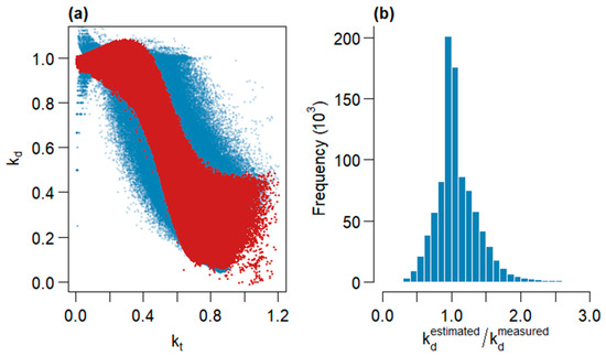
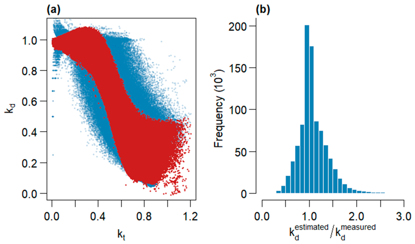
The performance of the proposed formulation for () is illustrated in Figure 1a. Figure 1a shows the measured (in blue) and estimated (in red) diffuse fractions as a function of the clearness index (kt). The close correspondence between the two distributions demonstrates that the proposed rational function model reproduces the observed variation in the diffuse fraction over a broad range of atmospheric conditions. Figure 1b presents the distribution of the estimated-to-measured (kd) ratio, which is concentrated around unity, further confirming the consistency of the model estimates with the measurements.
Figure 1.
(a) Values of diffuse fraction estimated (red) using the proposed model superimposed on the data from the D_FIT dataset (blue). (b) Histogram of the ratio between the estimated and measured diffuse fractions.
2.2.3. Graphical Analysis of Model Behavior
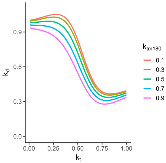
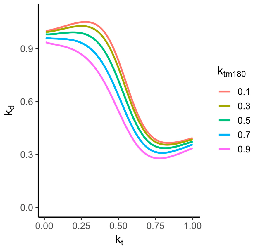
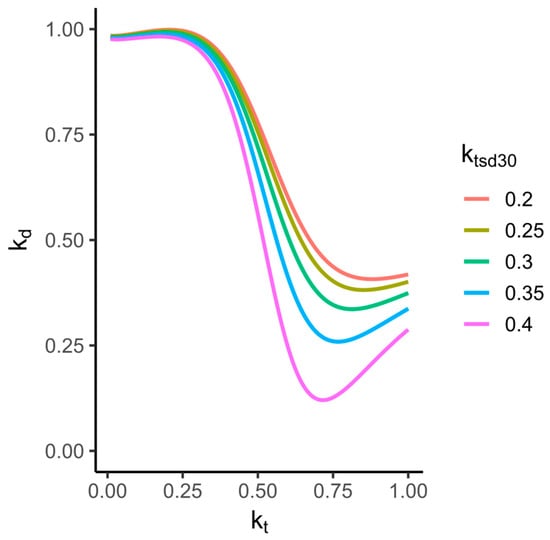
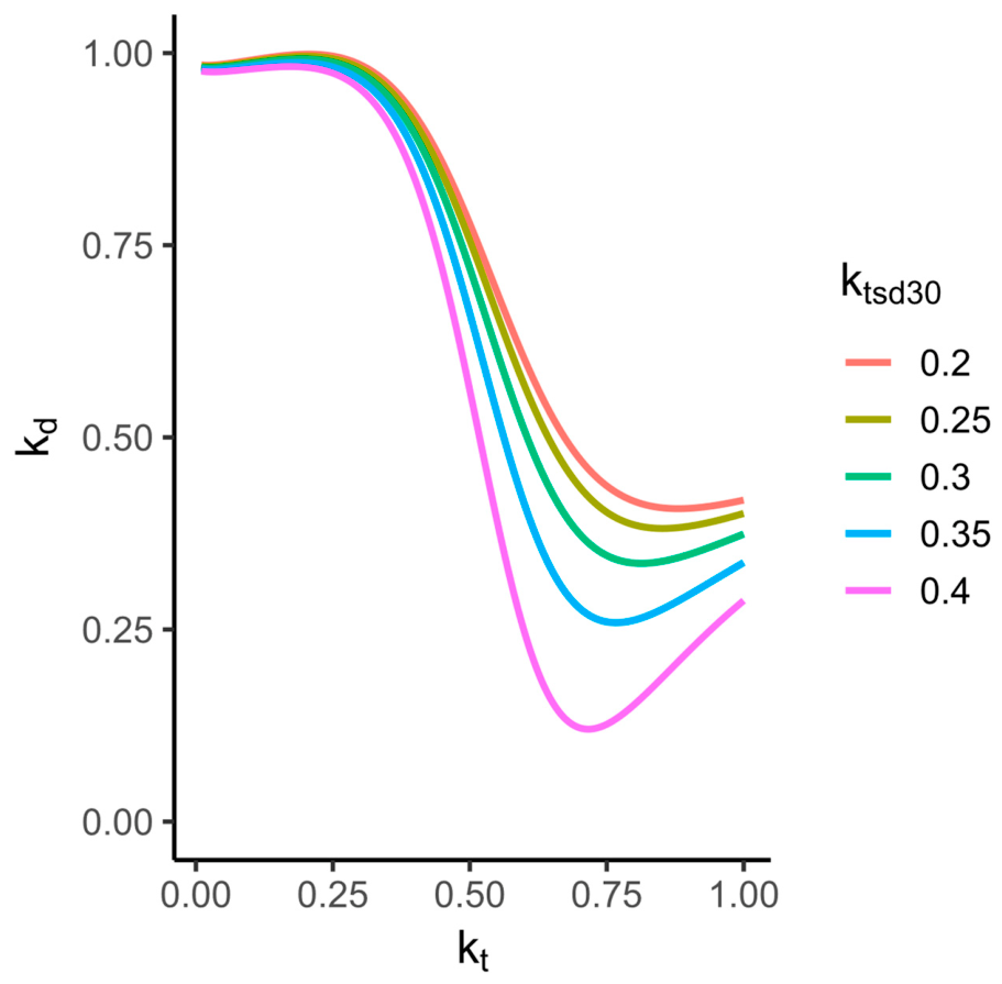
To gain further insight into the behavior of the proposed model, a graphical analysis of model behavior was performed by examining the variation in the estimated diffuse fraction () with the clearness index (kt) while varying the other predictors individually. For each analysis, selected predictors were fixed at representative values, whereas one predictor was varied over a prescribed range. Four cases were considered, corresponding to the 30-min mean clearness index, (), the 180-min mean clearness index, (), the 30-min standard deviation of the clearness index, (), and the solar zenith angle, cos θz. This analysis allows the individual influence of these predictors on the modeled (kd) to be visualized and provides insight into the behavior of the proposed mathematical formulation across different atmospheric and geometric conditions.
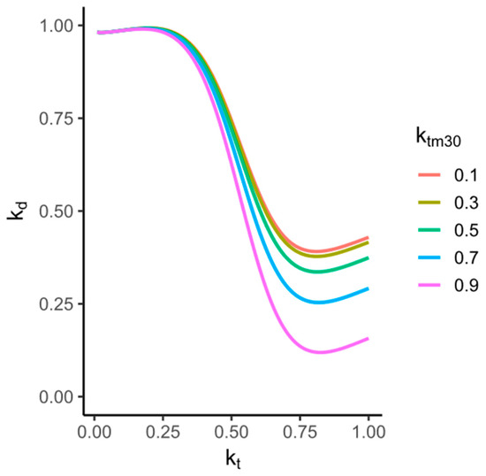
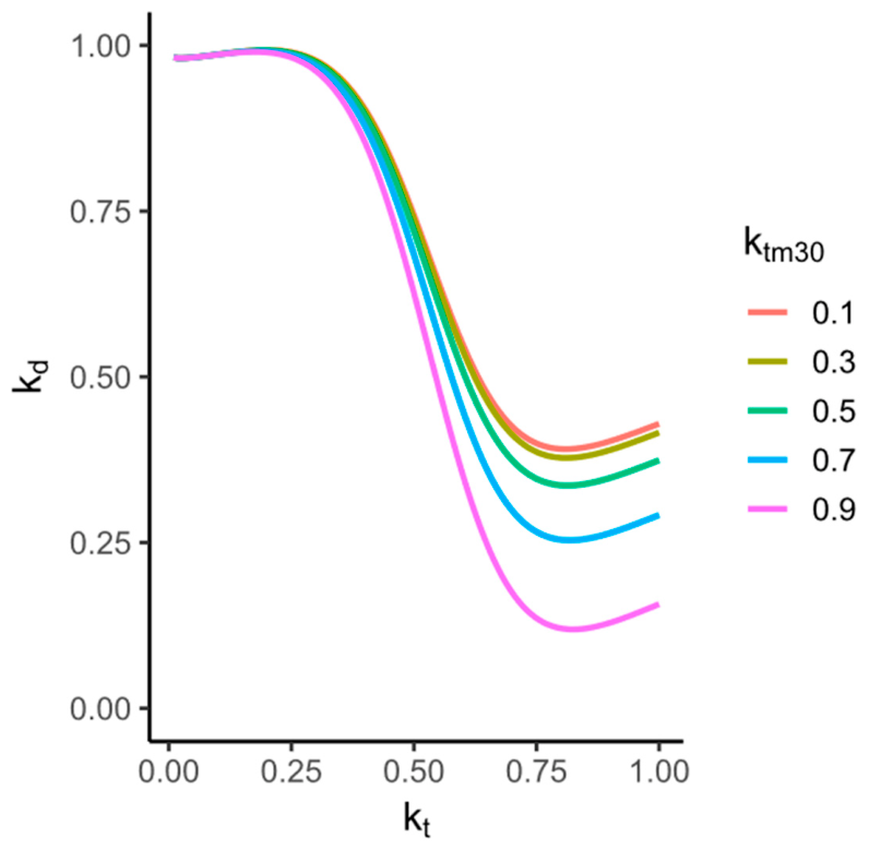
Figure 2 illustrates the dependence of the estimated diffuse fraction, (), on the clearness index, (kt), for different values of the 30-min moving average, (), while the remaining predictors are kept constant at (), (), and (cos θz = 2/3). The influence of () is relatively small at low values of (kt), whereas it becomes increasingly pronounced as (kt) increases. This behavior is consistent with the structure of the proposed model, in which () contributes through a term involving the product (kt ). Thus, the effect of the recent temporal evolution of atmospheric conditions becomes more important under relatively clear-sky conditions, when (kt) is high.
Figure 2.
Dependence of the estimated diffuse fraction, (kd), on the clearness index, (kt), for different values of the 30-min moving average of the clearness index, (), with the remaining predictors fixed at (), (), and (cos θz = 2/3).
Figure 3 illustrates the dependence of the estimated diffuse fraction, (), on the clearness index, (kt), for different values of the 180-min moving average, (), while the remaining predictors are kept constant at (), (), and (cos θz = 2/3). Increasing () from 0.1 to 0.9 produces a systematic downward shift in the (kd) curves, with approximately the same magnitude over the considered range of (kt). Thus, unlike the 30-min moving average, whose influence becomes more pronounced at higher (kt), the 180-min moving average affects the estimated diffuse fraction relatively uniformly across the range of clearness index values. The result indicates that the longer-term evolution of atmospheric conditions contributes to the estimation of (kd) under both cloudy and clear-sky conditions, irrespective of the instantaneous (kt) value. Moreover, the clearer the sky has been over the past three hours, the lower the estimated diffuse fraction.
Figure 3.
Dependence of the estimated diffuse fraction, (kd), on the clearness index, (kt), for different values of the 180-min moving average of the clearness index, (), with the remaining predictors fixed at (), (), and (cos θz = 2/3).
Figure 4 illustrates the dependence of the estimated diffuse fraction, (), on the clearness index, (kt), for different values of the 30-min standard deviation, (), while the remaining predictors are kept constant at (), (), and (cos θz = 2/3). The influence of () is relatively small at low values of (kt), whereas it becomes increasingly pronounced as (kt) increases. The effect of the recent variability of atmospheric conditions becomes more important under relatively clear-sky conditions, when (kt) is high.
Figure 4.
Dependence of the estimated diffuse fraction, (kd), on the clearness index, (kt), for different values of the 30-min standard deviation, (), with the remaining predictors fixed at (), (), and (cos θz = 2/3).
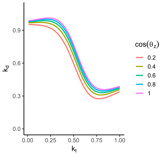
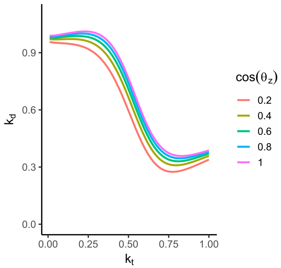
Figure 5 illustrates the dependence of the estimated diffuse fraction, (), on the clearness index, (kt), for different values of the zenith angle, (cos θz), while the remaining predictors are kept constant at (), (), and (). As (cos θz) increases from 0.2 to 1, the (kd) curves exhibit a systematic upward shift, with a relatively similar magnitude over the considered range of (kt). Thus, the zenith angle effect remains significant under both cloudy and clear-sky conditions, irrespective of the (kt) values. The uniform displacement of the curves indicates that the geometric effect represented by (cos θz) acts largely independently of (kt) in the proposed formulation.
Figure 5.
Dependence of the estimated diffuse fraction, (kd), on the clearness index, (kt), for different values of the zenith angle, (cos θz), with the remaining predictors fixed at (), (), and ().
3. Results
The performance of the proposed separation model was evaluated in two complementary stages. First, its predictive performance was assessed using one year of radiometric measurements from 25 BSRN stations, providing a broad validation across diverse atmospheric and climatic conditions. The validation dataset includes both stations also used for model development, for which observations from different years were used, and stations that were not involved in model development. Thus, the former provides a cross-year validation, while the latter provides an assessment at previously unseen stations. Second, the proposed model was compared with six established analytical models and three machine-learning models reported in a recent study based on measurements from ten BSRN stations [25]. This second analysis provides an independent benchmark against both classical and machine-learning approaches.
3.1. Validation of the Proposed Separation Model Across 25 BSRN Stations
The predictive performance of the proposed model was evaluated using the D_TEST dataset, consisting of one year of radiometric measurements from 25 BSRN stations. The geographical distribution and main characteristics of the test stations are summarized in Table 2. For the stations also included in D_FIT, namely GOB and PAY, the test observations correspond to years different from the year used for model development (2022). These data were therefore not used for model fitting and provide a cross-year validation of the proposed model. The remaining stations in D_TEST were not used for model development and provide validation at previously unseen stations.
Table 2.
Overview of the radiometric stations used in D_TEST, including their geographic coordinates and the number of observations before and after quality control.
The performance of the proposed separation model was evaluated using three statistical metrics: the normalized root mean square error (nRMSE), the normalized mean bias error (nMBE), and the coefficient of determination (R2). These metrics provide complementary information on the magnitude of the estimation errors, the systematic bias, and the overall agreement between estimated and measured values, respectively. The metrics were calculated separately for the diffuse horizontal irradiance (DHI) and direct normal irradiance (DNI).
The normalized root mean square error is defined as
where (N) is the number of observations, (yi) and (mi) are the estimated and measured values, respectively.
The normalized mean bias error is calculated as
The coefficient of determination is given by
where is the mean of measured values.
Table 3 summarizes the RMSE, nRMSE, nMBE, and (R2) values obtained at the 25 BSRN stations for the diffuse and direct components estimated with the proposed separation model.
Table 3.
Normalized root mean square error (nRMSE), normalized mean bias error (nMBE), and R2, for the estimation of direct-normal (DNI) and diffuse (DHI) irradiance using the proposed model at each station.
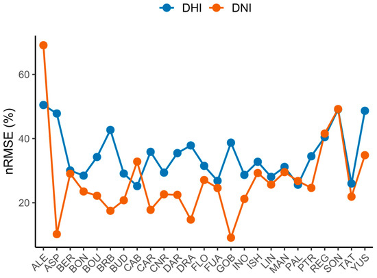
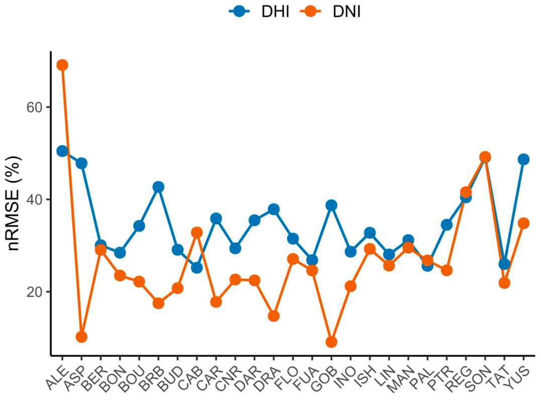
The nRMSE values reported in Table 3 for the diffuse and direct components are graphically illustrated in Figure 6 for the 25 BSRN stations. The figure facilitates the comparison of the model performance across stations and between the two irradiance components. It should be noted that errors in DHI can propagate into the estimated DNI through the closure equation,
Figure 6.
nRMSE obtained for the estimated DHI and DNI using the proposed separation model across the 25 BSRN stations in the (D_TEST) dataset.
Consequently, an error in DHI is amplified by the factor 1/cos θz, particularly at large solar zenith angles corresponding to low solar elevations. Thus, relatively small errors in DHI may result in larger errors in DNI, especially for observations at low solar elevations. This error-propagation effect should be considered when interpreting the station-dependent performance of the direct component.
The largest error was obtained at ALE, where the nRMSE for DNI reached 69.10%, whereas the lowest DNI nRMSE, 9.11%, was obtained at GOB. The relatively good performance at GOB may be partly related to the fact that one of the four years included in the (D_FIT) dataset was recorded at the same station, although from a different year than that used for testing. Thus, the model development dataset includes radiometric data representative of the local atmospheric and climatic characteristics of GOB. In contrast, ALE is located at a very high latitude (82.49° N), associated with markedly different solar geometry and seasonal conditions compared with those represented in the model development dataset. In addition, ALE exhibits a relatively high DHI error (nRMSE = 50.46%), which may contribute to the larger DNI error through the closure equation, particularly at large solar zenith angles. Similarly, the relatively high DNI errors observed at SON and REG (49.90% and 41.55%, respectively) are accompanied by comparatively high DHI errors (49.11% and 40.45%), suggesting that error propagation from the diffuse component may contribute to the station-dependent performance of the derived DNI.
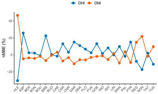
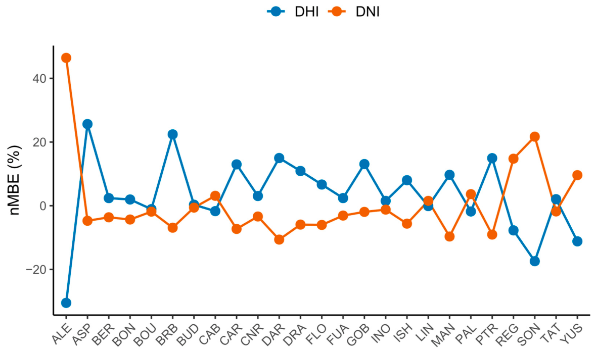
The nMBE values reported in Table 3 are shown graphically in Figure 7 for the diffuse and direct irradiance components across the 25 BSRN stations. The figure provides an overview of the systematic bias of the proposed model and allows the bias characteristics of the two estimated components to be compared across the different stations.
Figure 7.
nMBE obtained for the estimated DHI and DNI using the proposed separation model across the 25 BSRN stations in the (D_TEST) dataset.
As observed by nRMSE, the largest biases were obtained at ALE. For this station, the proposed model yielded an nMBE of +46% for DNI and −30% for DHI, indicating a substantial overestimation of the direct component and underestimation of the diffuse component. For the remaining 24 stations, the nMBE values were considerably lower, ranging from −17.42% for DHI at SON to +25.64% for DHI at ASP. Overall, these results indicate a substantially more balanced model performance across most of the test stations, with ALE representing a clear outlier in terms of systematic bias. The opposite signs of the DNI and DHI biases at ALE are also consistent with the propagation of errors through the closure equation, whereby an underestimation of DHI can contribute to an overestimation of the derived DNI.
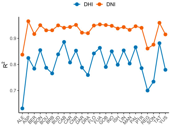
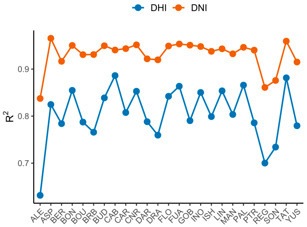
The corresponding (R2) values for the diffuse and direct irradiance components across the 25 BSRN stations are presented in Figure 8. The (R2) values indicate the proportion of the variability in the measured irradiance that is explained by the proposed model.
Figure 8.
Coefficient of determination (R2) obtained for the estimated DHI and DNI using the proposed separation model across the 25 BSRN stations in the (D_TEST) dataset.
Figure 8 shows that the proposed model generally achieves higher (R2) values for DNI than for DHI across most of the 25 BSRN stations, indicating that a larger proportion of the variability in the direct component is captured by the model. As observed by the other performance metrics, the lowest (R2) values are obtained at ALE, with values of 0.837 for DNI and 0.631 for DHI. The next lowest (R2) values for DNI are found at REG (0.860), located in Canada at a latitude of approximately 50°, and at SON (0.875), a high-altitude mountain station located above 3000 m. The relatively lower performance at SON may be associated with the high short-term variability of atmospheric conditions at this site. The reduced performance at REG and ALE may likewise reflect atmospheric and solar conditions that are less represented in the model development dataset. These interpretations should be regarded as possible explanations, as the specific contribution of these factors was not separately investigated in the present study.
3.2. Comparison with Existing Empirical and Machine-Learning Models
To further assess the performance of the proposed separation model, a direct comparison was made with the results reported by Rajagukguk and Lee [25] for ten BSRN stations. Their study evaluated six established empirical separation models and three machine-learning models, namely XGBoost, LightGBM, and CatBoost. The same test years used in their study were considered here, and the radiometric data were subjected to the same quality-control procedure. Thus, the nRMSE values obtained with the proposed model are evaluated under the same test periods and quality-control criteria as those used in their study, providing a consistent basis for comparison with the reported results.
The six empirical decomposition models selected by Rajagukguk and Lee [25] were developed using minute-resolution data and represent recent approaches to the estimation of diffuse and direct solar irradiance. All six models use the clearness index, (kt), as a fundamental predictor, while additional models incorporate solar zenith or elevation angle, atmospheric or seasonal time parameters (AST), moving averages of the clearness index, and clear-sky irradiance. The Engerer2 [10] and Engerer4 [27] models use (kt), solar zenith angle, (AST), and the derived parameters (∆ktc) and (kde). Every model [28] combines (kt) with solar elevation angle, (AST), daily clearness index, and a three-point moving average of (kt). The Starke2 [11] and Starke3 [12] models additionally incorporate clear-sky irradiance and hourly clearness-index information, while the Yang4 [14] model extends the Engerer-type formulation by including the hourly diffuse fraction derived from Engerer2. The input variables used by these models are summarized in Table 4 of the reference study [25].
The reference study also evaluated three machine-learning models based on gradient-boosting algorithms: XGBoost, LightGBM, and CatBoost [29]. These models were trained using the first two years of measurements at each station and subsequently evaluated using the third year. Unlike the empirical models, the machine-learning approaches can learn complex nonlinear relationships between the input predictors and the irradiance components directly from the training data. Their results therefore provide a relevant benchmark for assessing whether the simpler mathematical formulation proposed in the present study can achieve competitive performance without station-specific model training.
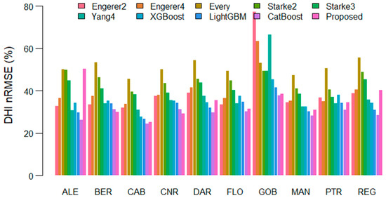
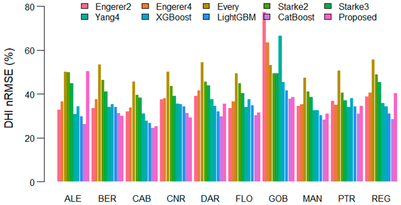
Figure 9 presents the nRMSE values obtained for DHI at the ten BSRN stations, comparing the proposed model with the six empirical models and the three machine-learning models considered in the reference study [25]. The proposed model shows competitive performance across the different stations. In particular, it achieves the lowest nRMSE at BER and CNR, outperforming all nine reference models at these stations. At CAB, DAR, FLO, GOB, and MAN, the proposed model performs better than all six empirical models, although some of the machine-learning models provide lower errors. These results indicate that the proposed mathematical formulation can achieve competitive performance relative to considerably more complex approaches, despite using a single set of coefficients and requiring no station-specific training.
Figure 9.
Comparison of DHI nRMSE values obtained with the considered decomposition models across the ten BSRN stations. Each group represents a station, while the individual bars correspond to the evaluated models.
The least favorable performance is observed at ALE, where the proposed model has the highest nRMSE among all models considered. At REG, it ranks second from the bottom, indicating reduced performance under the atmospheric conditions characteristic of this station. At PTR, however, the proposed model provides a reasonably competitive result. Overall, the comparison shows that the proposed model does not consistently outperform the reference approaches, but it achieves competitive or superior performance at a substantial number of stations, particularly when compared with the empirical models.
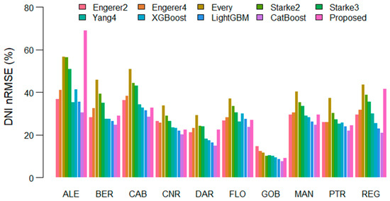
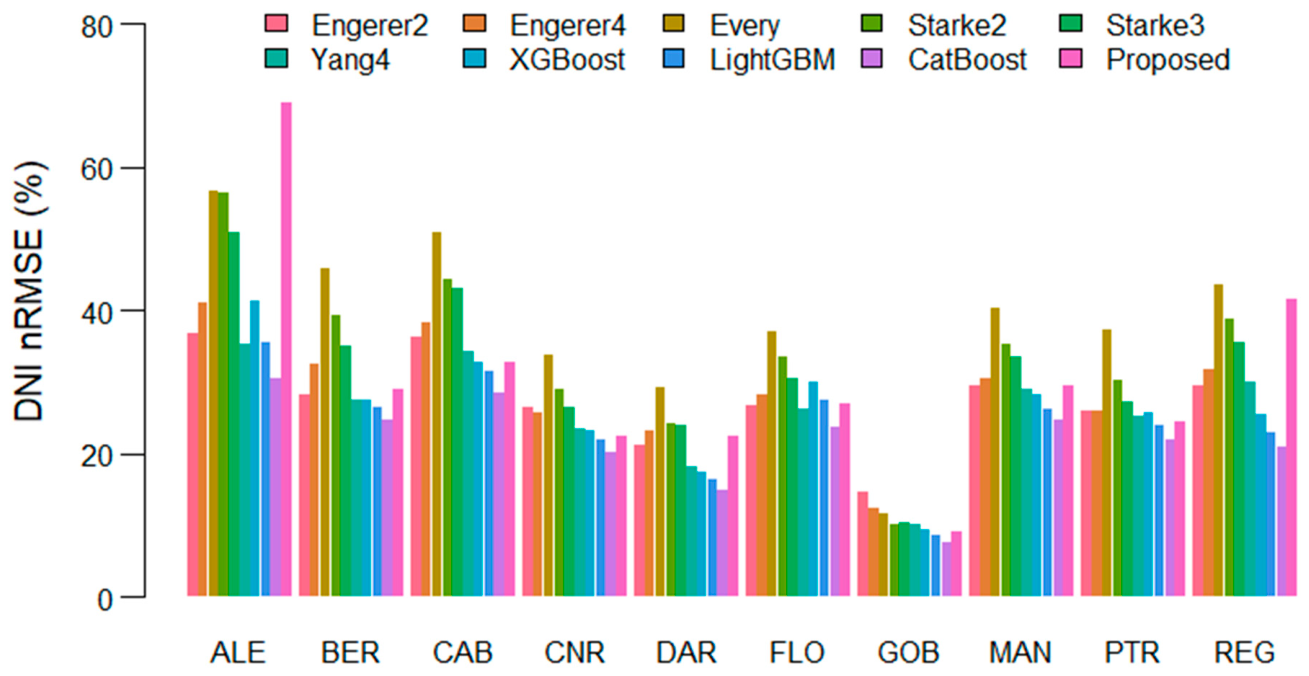
Figure 10 presents the nRMSE values obtained for DNI at the ten BSRN stations. The proposed model shows competitive performance across most of the stations. In particular, at CAB, CNR, GOB, and PTR, it achieves lower nRMSE values than all six empirical models as well as the XGBoost model. These results indicate that the proposed mathematical formulation can provide competitive estimates of the direct irradiance component despite its simpler structure and the absence of station-specific training.
Figure 10.
Comparison of DNI nRMSE values obtained with the considered decomposition models across the ten BSRN stations. Each group represents a station, while the individual bars correspond to the evaluated models.
As observed by DHI, the least favorable performance is obtained at ALE, where the proposed model exhibits the highest nRMSE among all models considered. At REG, it ranks second from the bottom. At the remaining stations, the proposed model provides reasonably competitive results, although some of the reference models achieve lower errors. Overall, the results indicate that the proposed model performs particularly well at several evaluated stations and remains competitive with established empirical and machine-learning approaches for DNI estimation. These findings support the competitiveness of the proposed formulation for the evaluated stations and test periods, but do not establish its superiority under all climatic or atmospheric conditions.
4. Conclusions
A rational function model was proposed for the separation of global solar irradiance into its diffuse and direct components. The model estimates the diffuse fraction using only information derived from global irradiance measurements and solar geometry, incorporating the instantaneous clearness index together with its short- and longer-term temporal characteristics and short-term variability. Unlike many recently developed separation models based on logistic formulations or machine learning algorithms, the proposed approach is described by a single mathematical equation with one set of coefficients and does not require station-specific training.
The sensitivity analysis showed that the model responds consistently to variations in the predictor variables. The 30-min moving average of the clearness index has an increasingly pronounced effect at high clearness index values, whereas the 180-min moving average mainly produces a downward shift in the estimated diffuse fraction. The solar zenith angle effect is manifested primarily as an upward shift in the diffuse fraction with increasing solar elevation, while the influence of the short-term variability of the clearness index reflects the changing atmospheric conditions.
The model was independently evaluated using one year of measurements from 25 BSRN stations. The results demonstrate that the proposed formulation provides generally consistent estimates of both DHI and DNI, although its performance depends on the atmospheric and climatic characteristics of the station. The largest errors and biases were observed at ALE, while comparatively lower performance was also found at REG and SON. In contrast, the model showed good performance at a number of stations, including GOB, where the model development dataset contained measurements from a different year at the same site.
A direct comparison with six empirical decomposition models and three machine-learning models was also made for ten BSRN stations using the same test years and quality control procedure as the reference study. For DHI, the proposed model outperformed all nine reference models at BER and CNR and all six empirical models at CAB, DAR, FLO, GOB, and MAN. For DNI, it outperformed all six empirical models and XGBoost at CAB, CNR, GOB, and PTR. Although the proposed model does not systematically achieve the lowest error at every station, these results demonstrate that a relatively simple mathematical formulation can provide competitive performance compared with both established empirical models and machine-learning approaches.
Overall, the results indicate that the proposed rational function formulation represents a useful alternative for the separation of global solar irradiance into its diffuse and direct components. Its main advantages are its compact mathematical form, the use of predictors derived exclusively from GHI measurements and solar geometry, a single globally defined set of coefficients, and the absence of station-specific model training. These characteristics make the model attractive for applications where a transparent, computationally simple, and broadly applicable separation method is preferred over more complex data-driven approaches.
Author Contributions
Conceptualization, E.P. and A.K.; methodology, E.P.; software, A.K.; validation, E.P. and A.K.; formal analysis, E.P.; investigation, E.P.; resources, E.P.; data curation, A.K.; writing—original draft preparation, A.K.; writing—review and editing, E.P.; visualization, E.P.; supervision, E.P. All authors have read and agreed to the published version of the manuscript.
Funding
This research was funded by a grant from the Ministry of Education and Research, CCCDI–UEFISCDI, project number PN-IV-P6-6.1-CoEx-2024-0154, within PNCDI IV.
Data Availability Statement
The data presented in the study are openly available in the Baseline Solar Radiation Network: https://bsrn.awi.de/ (accessed on 12 September 2026).
Conflicts of Interest
The authors declare no conflicts of interest.
Abbreviations
The following abbreviations are used in this manuscript:
| BSRN | Baseline Surface Radiation Network |
| DHI | Diffuse horizontal irradiance |
| DNI | Direct normal irradiance |
| GHI | Global horizontal irradiance |
References
- Yang, D. Estimating 1-min beam and diffuse irradiance from the global irradiance: A review and an extensive worldwide comparison of latest separation models at 126 stations. Renew. Sustain. Energy Rev. 2022, 159, 112195. [Google Scholar] [CrossRef] [Scilit]
- Gueymard, C.A.; Ruiz-Arias, J.A. Extensive worldwide validation and climate sensitivity analysis of direct irradiance predictions from 1-min global irradiance. Sol. Energy 2016, 128, 1–30. [Google Scholar] [CrossRef] [Scilit]
- Martin János Mayer, M.J.; Gróf, G. Extensive comparison of physical models for photovoltaic power forecasting. Appl. Energy 2021, 283, 116239. [Google Scholar] [CrossRef] [Scilit]
- Liu, B.Y.H.; Jordan, R.C. The interrelationship and characteristic distribution of direct, diffuse and total solar radiation. Sol. Energy 1960, 4, 1–19. [Google Scholar] [CrossRef] [Scilit]
- Erbs, D.G.; Klein, S.A.; Duffie, J.A. Estimation of the diffuse radiation fraction for hourly, daily and monthly-average global radiation. Sol. Energy 1982, 28, 293–302. [Google Scholar] [CrossRef] [Scilit]
- Reindl, D.T.; Beckmann, W.A.; Duffie, J.A. Diffuse Fraction Correlations. Sol. Energy 1990, 45, 1–7. [Google Scholar] [CrossRef] [Scilit]
- Skartveit, A.; Olseth, J.A.; Tuft, M.E. An hourly diffuse fraction model with correction for variability and surface albedo. Sol. Energy 1998, 63, 173–183. [Google Scholar] [CrossRef] [Scilit]
- Boland, J.; Ridley, B.; Brown, B. Models of diffuse solar radiation. Renew. Energy 2008, 33, 575–584. [Google Scholar] [CrossRef] [Scilit]
- Ridley, B.; Boland, J.; Lauret, P. Modelling of diffuse solar fraction with multiple predictors. Renew. Energy 2010, 35, 478–483. [Google Scholar] [CrossRef] [Scilit]
- Engerer, N.A. Minute resolution estimates of the diffuse fraction of global irradiance for southeastern Australia. Sol. Energy 2015, 116, 215–237. [Google Scholar] [CrossRef] [Scilit]
- Starke, A.R.; Lemos, L.F.L.; Boland, J.; Cardemil, J.M.; Colle, S. Resolution of the cloud enhancement problem for one-minute diffuse radiation prediction. Renew. Energy 2018, 125, 472–484. [Google Scholar] [CrossRef] [Scilit]
- Starke, A.R.; Lemos, L.F.L.; Barni, C.M.; Machado, R.D.; Cardemil, J.M.; Boland, J.; Colle, S. Assessing one-minute diffuse fraction models based on worldwide climate features. Renew. Energy 2021, 177, 700–714. [Google Scholar] [CrossRef] [Scilit]
- Abreu, E.F.M.; Canhoto, P.; Costa, M.J. Prediction of diffuse horizontal irradiance using a new climate zone model. Renew. Sustain. Energy Rev. 2019, 110, 28–42. [Google Scholar] [CrossRef] [Scilit]
- Yang, D. Temporal-resolution cascade model for separation of 1-min beam and diffuse irradiance. J. Renew. Sustain. Energy 2021, 13, 056101. [Google Scholar] [CrossRef] [Scilit]
- Rodríguez, E.; Cornejo-Ponce, L.; Cardemil, J.M.; Starke, A.R.; Droguett, E.L. Estimation of one-minute direct normal irradiance using a deep neural network for five climate zones. Renew. Sustain. Energy Rev. 2023, 183, 113486. [Google Scholar] [CrossRef] [Scilit]
- Rodríguez, E.; Droguett, E.L.; Cardemil, J.M.; Starke, A.R.; Cornejo-Ponce, L. Enhancing the estimation of direct normal irradiance for six climate zones through machine learning models. Renew. Energy 2024, 231, 120925. [Google Scholar] [CrossRef] [Scilit]
- Ruiz-Arias, J.A.; Domínguez, E.; Gueymard, C.A. Comparison of conventional and simple artificial neural network models for high-performance separation of global solar irradiance components at minutely resolution. Sol. Energy 2025, 301, 113878. [Google Scholar] [CrossRef] [Scilit]
- Gueymard, C.A. REST2: High-performance solar radiation model for cloudless-sky irradiance, illuminance, and photosynthetically active radiation—Validation with a benchmark dataset. Sol. Energy 2008, 82, 272–285. [Google Scholar] [CrossRef] [Scilit]
- Paulescu, E.; Paulescu, M. A new clear sky solar irradiance model. Renew. Energy 2021, 179, 2094–2103. [Google Scholar] [CrossRef] [Scilit]
- Yang, D.; Gu, Y.; Mayer, M.J.; Gueymard, C.A.; Wang, W.; Kleissl, J.; Li, M.; Chu, Y.; Bright, J.M. Regime-dependent 1-min irradiance separation model with climatology clustering. Renew. Sustain. Energy Rev. 2024, 189, 113992. [Google Scholar] [CrossRef] [Scilit]
- Rodríguez, E.; Cardemil, J.M.; Droguett, E.L. Developing temporal clustering for identifying solar radiation zones to improve separation models. Renew. Energy 2026, 256, 123809. [Google Scholar] [CrossRef] [Scilit]
- Paulescu, E.; Paulescu, M. Minute-Scale Models for the Diffuse Fraction of Global Solar Radiation Balanced between Accuracy and Accessibility. Appl. Sci. 2023, 13, 6558. [Google Scholar] [CrossRef] [Scilit]
- Driemel, A.; Augustine, J.; Behrens, K.; Colle, S.; Cox, C.; Cuevas-Agull’o, E.; Denn, F.M.; Duprat, T.; Fukuda, M.; Grobe, H.; et al. Baseline surface radiation network (BSRN): Structure and data description (1992–2017). Earth Syst. Sci. Data 2018, 10, 1491–1501. [Google Scholar] [CrossRef] [Scilit]
- Yang, D.; Yagli, G.M.; Quan, H. Quality control for solar irradiance data. In Proceedings of the International Conference on Innovative Smart Grid Technologies (ISGT Asia 2018), Singapore, 22–25 May 2018; IEEE: Piscataway, NJ, USA, 2018; pp. 208–213. [Google Scholar] [CrossRef] [Scilit]
- Rajagukguk, R.A.; Lee, H. Application of explainable machine learning for estimating direct and diffuse components of solar irradiance. Sci. Rep. 2025, 15, 7402. [Google Scholar] [CrossRef] [Scilit]
- Vuilleumier, L.; Hauser, M.; Félix, C.; Vignola, F.; Blanc, P.; Kazantzidis, A.; Calpini, B. Accuracy of ground surface broadband shortwave radiation monitoring. J. Geophys. Res.-Atmos. 2014, 119, 13838–13860. [Google Scholar] [CrossRef] [Scilit]
- Bright, J.M.; Engerer, N.A. Engerer2: Global re-parameterisation, update, and validation of an irradiance separation model at different temporal resolutions. J. Renew. Sustain. Energy 2019, 11, 033701. [Google Scholar] [CrossRef] [Scilit]
- Every, J.P.; Li, L.; Dorrell, D.G. Köppen-Geiger climate classification adjustment of the BRL diffuse irradiation model for Australian locations. Renew. Energy 2020, 147, 2453–2469. [Google Scholar] [CrossRef] [Scilit]
- Aksoy, N.; Genc, I. Predictive models development using gradient boosting based methods for solar power plants. J. Comput. Sci. 2023, 67, 101958. [Google Scholar] [CrossRef] [Scilit]

Disclaimer/Publisher’s Note: The statements, opinions and data contained in all publications are solely those of the individual author(s) and contributor(s) and not of MDPI and/or the editor(s). MDPI and/or the editor(s) disclaim responsibility for any injury to people or property resulting from any ideas, methods, instructions or products referred to in the content. |
© 2026 by the authors. Licensee MDPI, Basel, Switzerland. This article is an open access article distributed under the terms and conditions of the Creative Commons Attribution (CC BY) license.