


Abstract
Azimuthal temperature biases in multi-level tower-mounted sensors have long been reported, yet their underlying physical causes remain unclear. In particular, three candidate mechanisms—flow blockage, structural-geometry effects, and instrument-to-instrument differences in radiative sensitivity—have rarely been disentangled within a single observational experiment. Here, we address this gap by using a 100 m lattice tower at the Shouxian National Climate Observatory (32.5° N, 116.8° E), which has base and top widths of 10.0 m and 2.0 m, respectively. East–west symmetric dual temperature sensors and independent bilateral anemometers were installed at 34, 50, 65, and 80 m, with an additional reference anemometer at 95 m. On 12 May 2025, the complete probe-and-shield assembly at 50 m was reversed east–west, whereas the other three levels remained unchanged as negative controls, thereby establishing a difference-in-differences (DID) framework. Using the top-mounted reference wind direction, the bilateral wind-speed difference shows no statistically significant shadow sector at any level, allowing us to reject the flow-blockage (tower-shadow) hypothesis. The structural baseline bias S(z) of the three un-swapped decreases monotonically in magnitude with height (from −0.92 °C at 34 m to −0.28 °C at 80 m) and tracks the height-dependent tower geometry, proxied by the face width W(z), linearly, with stable day–night behavior—pointing to a geometric/orientational origin. After the swap, the 50 m bias amplifies to 3–18 times the baseline and reverses seasonally; the inter-instrument difference in daytime shortwave response is significant (Δα = +46.27 × 10⁻³ °C/(MJ m−2 d−1), 95% CI [+5.71, +91.30]), whereas the nighttime net-longwave difference is directionally consistent but not significant (Δβ = +38.33 × 10⁻³ °C/(W m−2), 95% CI [−1.32, +70.78]). We conclude that instrument-swap-induced homogeneity breaks are more likely caused by inter-instrument differences in radiative-response sensitivity than by a constant offset. This finding has important implications for climate-network homogenization and for azimuthal quality control of tower-mounted sensors.
1. Introduction
As a fundamental variable in boundary-layer meteorology and climatology, the accuracy of air temperature measurements directly affects the reliability of weather analysis, climate monitoring, and numerical model evaluation. In operational practice, temperature sensors are housed in naturally ventilated radiation shields to avoid direct solar heating, yet the shield itself introduces a systematic bias. From an energy-balance perspective, daytime solar shortwave radiation is absorbed by the shield walls and converted to sensible heat [1,2]; the shield’s cooling efficiency depends on natural ventilation and longwave radiative exchange. When ventilation is restricted, the air inside the shield is continuously heated, and the sensor reads higher than the true air temperature [3]. Richardson [4] conducted multi-shield heating-error experiments confirming that this bias grows with incident irradiance and weakens with ambient wind speed, reaching magnitudes of about 1 °C. At night, the physical process reverses: the shield radiates net longwave energy toward the sky and cools below ambient, producing a negative bias [5]. This energy-balance framework carries an implicit, but insufficiently tested, inference—that shield cooling efficiency is further modulated by both the inflow conditions and the shield’s radiative properties. Consequently, when a temperature sensor is mounted beside a large obstacle such as a meteorological tower, an azimuthal observation bias can, in principle, arise through two independent pathways: flow blockage by the tower structure (the tower-shadow effect) and inter-instrument differences in radiative response. Yet these two pathways have rarely been tested and separated within the same experiment.
A growing body of methodological work has sought to correct radiation-shield temperature errors. Jin et al. [6] reconstructed the shield geometry for a naturally ventilated sensor using computational fluid dynamics (CFD) and reduced the root-mean-square error by roughly 40% under daytime conditions. Li et al. [7] trained a neural-network correction model on multi-season field data, achieving residual errors below 0.1 °C at moderate wind speeds. Sakalis [8] proposed an empirical daytime correction for naturally ventilated shields, while Yang et al. [9,10,11] developed a series of correction methods for typical shields such as the DTR503A and designed a low-cost, high-ventilation shield. Jin et al. [12] and Liu et al. [13] further advanced the design and experimental validation of high-accuracy naturally ventilated shields. In the wireless-sensor-network context, Sun et al. [14] and Wang et al. [15] developed solar-radiation-based temperature correction schemes. Notably, Lefevre et al. [16] recently demonstrated substantial sensor-to-sensor variability in radiation-shield errors that varies with irradiance and ventilation—providing direct theoretical support for the point that swapping identical instruments between positions can introduce a systematic step. Collectively, however, these studies assume the sensor is an isolated point measurement, excluding from their modeling framework the systematic error that arises from its azimuth relative to a nearby obstacle such as a tower.
Parallel developments in wind energy have produced a relatively mature framework for analyzing tower shadow and flow distortion. Orlando et al. [17] experimentally quantified the tower-shadow effect on anemometer readings. Lubitz and Michalak [18] and Lubitz [19] established experimental and theoretical models of tower shadow and proposed bilateral complementary anemometry. Farrugia and Sant [20,21] examined data-screening strategies for wind measurements near tubular masts and simulated the response of symmetrically mounted cup anemometers on lattice towers. The theory of flow-distortion effects on scalar-flux measurements traces back to Wyngaard [22], and McCaffrey et al. [23] identified tower-wake distortion using co-located sonic anemometers and lidar. Importantly, these methods were developed primarily for wind-speed measurement and have seldom been applied to the examination of temperature-sensor radiative errors or azimuthal biases. This exposes a clear gap: although azimuthal biases in tower-mounted multi-level temperature observations are long known, the three candidate mechanisms—flow blockage, structural-geometry differences, and inter-instrument differences in radiative sensitivity—have rarely been jointly tested within a single experimental framework.
Against this backdrop, we conducted a controlled instrument-swap experiment on a 100 m gradient tower at the Shouxian National Climate Observatory (32.5° N, 116.8° E). The tower is equipped with east–west symmetric, dual temperature sensors and independent bilateral anemometers at 34, 50, 65, and 80 m, as well as an additional reference anemometer at 95 m. On 12 May 2025, the entire probe, shield, and bracket assembly at 50 m was swapped east–west, while the other three levels remained in place as controls, forming a difference-in-differences (DID) identification framework. Our contributions are threefold: (1) using independent bilateral anemometry and the top reference wind direction, we empirically test and reject the flow-blockage hypothesis on a temperature-observing tower—a negative result that is itself methodologically informative and serves as a reference for similar tower-mounted observations; (2) we exploit the swap to separate, empirically, the structural-geometry effect from the instrument-individual effect, and, drawing on the construction drawings that give tower-face width W(z) as a function of height, we elevate ‘tower geometry’ from background description to a testable independent variable; (3) through dual-channel regression on daytime shortwave dose and nighttime net longwave radiation, we characterize the inter-instrument difference in radiative-response sensitivity, unifying the three candidate mechanisms within one experimental framework. These results directly inform the mechanisms behind homogenization breaks induced by instrument changes in climate networks and the optimization of network homogenization and tower-mounted azimuthal quality control.
2. Materials and Methods
2.1. Site, Tower, and Instrumentation
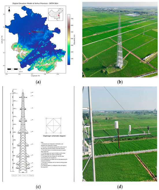
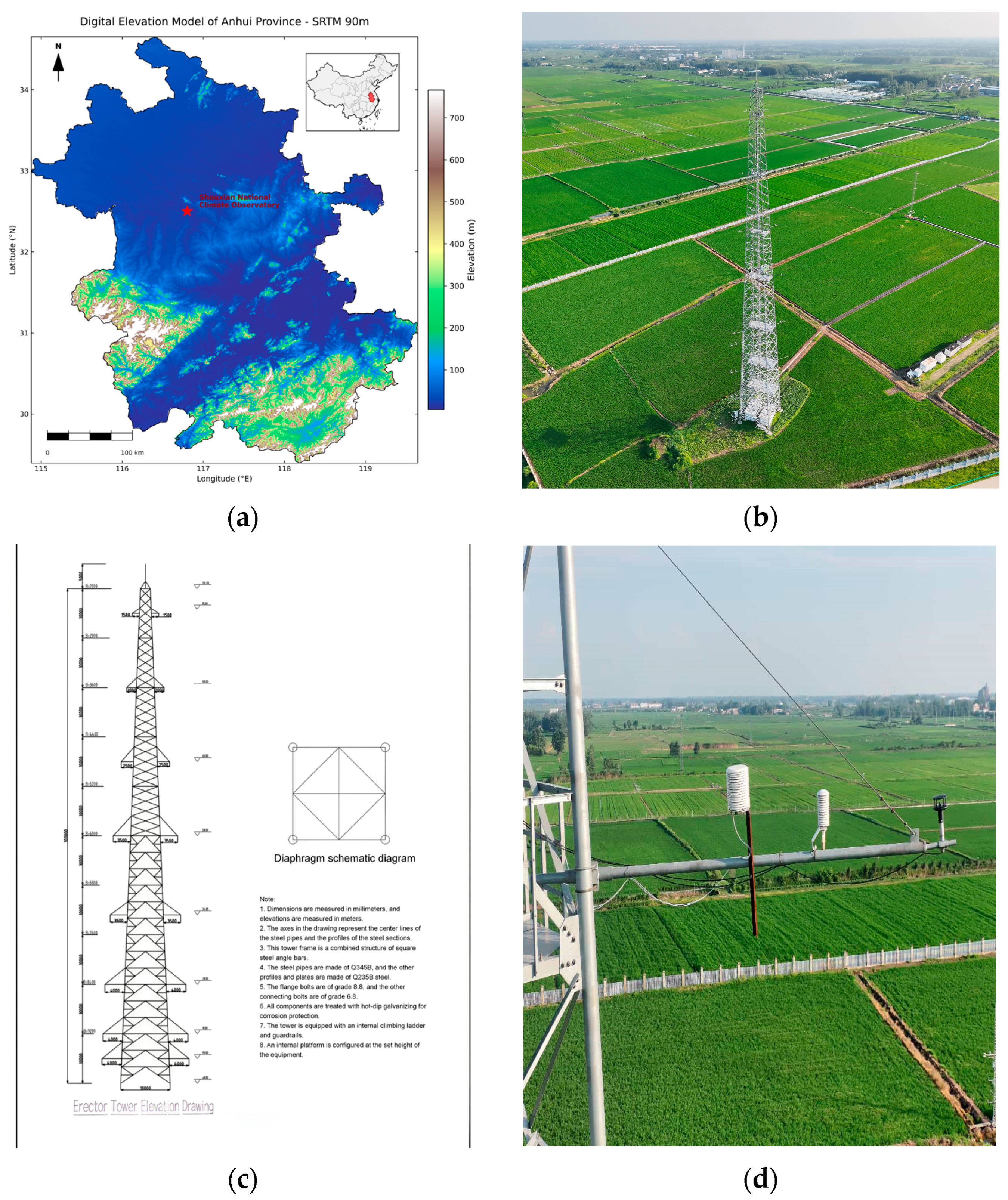
The observations were conducted at the Shouxian National Climate Observatory, located within the Huaihe River Basin Typical Agro-Meteorological Field Experiment Base under the China Meteorological Administration. The station lies at an elevation of 25 m in the central Huaihe River Basin, within a north-subtropical monsoon climate regime characterized by distinct seasons, a mean annual temperature of approximately 15.6 °C, annual precipitation of about 931 mm, and predominantly easterly winds. The station is situated within a uniformly agricultural landscape, characterized by flat, open terrain and the absence of tall structures within a 10 km radius, thereby meeting the World Meteorological Organization (WMO) representativeness criteria for observing stations [24]. The station location and its underlying surface conditions are illustrated in Figure 1a. The data record covers the period from 28 August 2022 to 7 May 2026, and all times are reported in Beijing Standard Time (BJT, UTC+8). The station location is shown in Figure 1a; a full-resolution version of this map is provided in Figure S1.
Figure 1.
(a) Station location: derived from the Anhui Province digital elevation model (SRTM 90 m); the color scale indicates elevation (m). A north arrow is placed at the upper left, a 100 km scale bar at the lower left, and a national-map inset (red dot marking the station’s position within China) at the upper right. The red marker indicates the Shouxian National Climate Observatory (32.5° N, 116.8° E, elevation 25 m). (b) Drone photograph of the 100 m lattice tower: the tower stands in homogeneous agricultural land with flat, open surroundings; the 34/50/65/80 m levels are east–west symmetric observation levels (50 m is the swap level), and an independent reference anemometer is mounted at 95 m. (c) General arrangement drawing of the tower structure (from the construction drawings, December 2020): the left panel is the elevation view (with segmented dimension annotations; base width 10.0 m, top width 2.0 m), and the lower right shows a cross-bracing schematic; the bottom text gives construction notes. (d) Detail of the observation-level boom and instrument mounting: the naturally ventilated radiation shield (white louvered housing at right, enclosing the HMP155A temperature–humidity probe) is fixed to the horizontal boom; the black device beside it is the WindSonic two-dimensional sonic anemometer. The background shows the agricultural underlying surface of the station. (Detailed information for Figure 1c can be found in the Supplementary Materials).
The observation tower is a 100 m-high quadrilateral lattice structure constructed from steel tubes and angle steel (construction drawings completed in December 2020; see Figure 1c). A full-resolution version of the general arrangement drawing is provided in Figure S2. The primary tubular members are made of Q345B steel, whereas the remaining components and plates use Q235B. Structural segments are connected by flanges, with flange bolts of grade 8.8 and other bolts of grade 6.8, and all steel members are protected against corrosion by hot-dip galvanizing. The tower is equipped with an internal ladder and service platforms at 65, 80, and 95 m, and the top section supports a lightning rod, down conductor, and grounding system. The structure is designed for a basic wind pressure of 0.65 kN/m2 (GB 50009-2001) [25], a seismic fortification intensity of 8 degrees (GB 50011-2001) [26], and an ice thickness of 10 mm, with a verticality tolerance better than 1/1500. The tower face width decreases linearly from 10.0 m at the base to 2.0 m at the top, corresponding to a reduction of 0.8 m for every 10 m of height.
where W(z) is the tower-face width (m) at height z (m). Equation (1) yields tower-face widths of approximately 7.28, 6.00, 4.80, and 3.60 m at the 34, 50, 65, and 80 m observation levels, respectively. Drone photographs of the tower and the general arrangement drawing from the construction documents are shown in Figure 1b,c, and the tower geometry and instrument-mounting parameters are summarized in Table 1.
W(z) = 10.0 − 0.08z,
Table 1.
Site and instrument configuration.
Along the tower diagonals, east–west symmetric booms are installed at 34, 50, 65, and 80 m. The boom length is L = 4.0 m at 34 and 50 m, and L = 3.5 m at 65 and 80 m. Together with the tower-face width from Equation (1), the relative boom extension L/W(z) increases monotonically with height from 0.55 (4.0/7.28) at 34 m to 0.97 (3.5/3.60) at 80 m, with intermediate values of 0.67 and 0.73 at 50 and 65 m, respectively. This ratio quantifies how far the sensors extend from the tower body.
At each level, both the east and west sides are equipped with a combined temperature–humidity probe (HMP155A, Vaisala, Vantaa, Finland; Pt100 thermometer, temperature accuracy ±0.17 °C, relative humidity accuracy ±1% RH) housed in identical, naturally ventilated radiation shields. Each side is also equipped with a two-dimensional sonic anemometer (WindSonic, Gill Instruments, Lymington, UK; wind-speed accuracy ±2%, wind-direction accuracy ±3°). The instrumental uncertainty of ΔT has two components. The random component, estimated empirically from first differences in the 1 min ΔT series (robust MAD), is 0.07–0.13 °C and averages down below 10−3 °C in all mean statistics; the systematic component—the fixed inter-probe calibration difference, bounded by ±0.24 °C (√2 × 0.17 °C; ±0.34 °C worst-case)—does not average down, but it cancels in all within-pair contrasts: it adds equally to the day and night means, leaves the radiative-response slopes unchanged, and shifts the 50 m swap contrast by at most 0.48 °C, far below the observed within-group changes of −1.9 to +2.3 °C (Section 3.3). It bounds the absolute magnitude of S(z)—|S(80 m)| = 0.28 °C is comparable to this envelope—but not the swap-attributed conclusions. In addition, an independent reference anemometer (boom length 1.5 m) installed at 95 m provides a wind-direction reference that is free from local obscuration at the observation levels. A separate radiation observatory is equipped with a CMP21 pyranometer (Kipp & Zonen, Delft, The Netherlands; spectral range 285–2800 nm, ISO 9060:2018 [27] spectrally flat Class A) to measure global shortwave radiation and a CGR3 pyrgeometer (Kipp & Zonen, Delft, The Netherlands; spectral range 4.5–42 µm, with an internal temperature sensor for dome-temperature correction) to measure longwave radiation; both instruments operate at a temporal resolution of 1 min. The radiation measurements are single-point station observations and are used as a regional proxy for the common incident radiation at all levels, rather than as directional measurements on each side. All variables are recorded by a CR-series data logger (Campbell Scientific, Logan, UT, USA), with a raw sampling rate of 1 Hz and output as 1 min statistics. All analyses are conducted at the 1 min scale, and daily and grouped statistics are aggregated from the 1 min records. Instrument-mounting details are shown in Figure 1d, and the overall configuration is summarized in Table 1.
2.2. Sensor-Swap Experiment Design and Data Processing
On 12 May 2025, a complete east–west instrument swap was carried out at the 50 m level: the entire eastern probe, shield, and bracket assembly was exchanged with the western assembly. Thus, the swapped unit included both the sensing element and its radiation-protection and mounting components, rather than only the probe. The instruments at 34, 65, and 80 m were left unchanged and served as negative-control levels. Data loss associated with manual operations and power-cycle restart on the swap date is treated as missing for the entire day. Accordingly, the pre-swap period is defined as 28 August 2022 to 11 May 2025 (approximately 2.7 years), and the post-swap period as 13 May 2025 to 7 May 2026 (about 1.0 year).
This design follows a difference-in-differences (DID) identification framework: if the east–west temperature difference is primarily driven by fixed tower-structure or flow-position effects, swapping the physical instruments should not change either the sign or the magnitude of the bias. In contrast, if the bias is determined by instrument-specific attributes (e.g., radiative-response sensitivity, calibration state), the 50 m bias should reverse or exhibit a discrete shift in magnitude after the swap, while the control levels should show no concurrent change. The design is consistent with the methodology of parallel observations and homogenization testing in climate networks [28,29,30]. Given the asymmetric pre/post window lengths and the autocorrelation of meteorological series, uncertainty estimates in all analyses use the day as the resampling unit (block bootstrap or moving-block bootstrap).
Data processing comprised the following steps: (1) Time alignment—temperature, wind, 95 m reference wind, and radiation observations at the four levels were paired by 1 min timestamp; any record with a missing element was discarded as a group. (2) Quality control—missing-value and range checks were applied sequentially (removing records outside instrument range or local climatic extremes, including physically implausible |ΔT| > 10 °C), and radiation data were checked for probe-temperature corrections and pyrgeometer dome-drift anomalies; radiation-response analyses further excluded days with fewer than 720 valid minutes. (3) Day–night and seasonal partitioning—the diurnal decomposition of the structural baseline and the DID grouping followed fixed clock hours: day 06:00–18:00, night 18:00–06:00 BJT; seasons were defined as winter (Dec–Feb), spring (Mar–May), summer (Jun–Aug), and autumn (Sep–Nov). In the radiative-response regression, daytime samples were minutes with solar elevation > 0 and GHI > 50 W m−2, and nighttime samples minutes with solar elevation < 0; solar elevation was computed minute-by-minute from station latitude and longitude using the standard NOAA solar-position algorithm (self-implemented). (4) Calm-wind screening—the nighttime radiative-response analysis used a 1 min wind-speed threshold of <2.0 m/s, with a 1.5 m/s threshold for sensitivity testing. All computations were performed in Python 3.10.20 (NumPy 2.2.5, pandas 2.3.3, SciPy 1.15.3), with a two-sided significance level of 0.05. To diagnose the seasonal sign reversal, the quality-controlled ΔT was additionally conditioned on the minute-wise solar azimuth, and correlated at the daily scale (day- and night-phase means) with solar noon elevation, daily shortwave dose, clearness index, wind speed, relative humidity, BSRN-measured surface albedo, and nighttime net longwave radiation; the un-swapped 65 m level served as a within-tower control.
2.3. Quantification of Azimuthal Bias
To test the mechanism that ‘tower flow blockage (tower shadow) causes east–west ventilation differences, which in turn produce azimuthal asymmetry in shield cooling efficiency, we draw on the concept of complementary anemometry from wind-energy metering [17,18,19,20,21,22,23] and adapt it to the problem of temperature-observation error. Specifically, we use the 95 m top reference wind direction θ95 as the angular reference—rather than taking the wind direction from the higher-speed side as a proxy—to avoid circular reasoning when inferring the obscured position from measurements that may themselves be locally affected by tower shadow. At each level, we then compute the east–west wind-speed difference:
where bin(θ) denotes a 10° wind-direction bin (with wrap-around handling across 0°/360°) boundary. The median ΔV within each bin is taken, and its 95% confidence interval is estimated by block bootstrap; ΔV/V95 normalized by the 95 m wind speed serves as a robustness metric. A bin is flagged as a significant shadow sector when its ΔV confidence interval excludes zero over a contiguous directional range and its sign matches the expectation derived from tower obstruction of the flow of that side. To quantify the detection capability of this negative test, we define the minimum detectable effect (MDE) as a persistent sectoral wind-speed deficit equal to twice the half-width of the widest bin confidence interval: such a deficit is detectable with ≈97.5% probability under a normal approximation (a deficit equal to a single half-width corresponds to ≈50%). The MDE is then compared with the 0.1 m s−1 resolution at which routine meteorological wind-speed observations are reported, as a meteorologically meaningful scale of relevance. This identification is carried out independently for all four levels. For the 50 m level, the analysis is additionally recomputed for the pre- and post-swap periods to verify that the swap does not modify the flow field at that level. Given that the L/W(z) ratio (0.55→0.97) increases with height, the sensor extends progressively farther beyond the tower face, implying that if the tower-shadow mechanism were operative, its influence should diminish with height and be strongest at the lowest levels. Comparing this expectation with the test results validates (or rejects) the tower-shadow hypothesis.
ΔV(θ) = median{V_east − V_west | θ95 ∈ bin(θ)},
Building on the framework, we define the east–west temperature difference ΔT(z, t) = T_east(z, t) − T_west(z, t). For all four levels, the structural baseline bias S(z) is defined as the arithmetic mean of the quality-controlled 1 min records of ΔT over the pre-swap period (28 August 2022 to 11 May 2025, a common baseline window for all four levels):
where W_pre is the set of N(z) valid 1 min ΔT records at level z within the pre-swap window (day and night minutes combined). The day- and night-specific baselines S_day(z) and S_night(z) used in the diurnal decomposition are defined analogously over the corresponding clock-hour subsets (Section 2.2). The uncertainty of S(z) is quantified by the block-bootstrap 95% confidence interval of the daily means (B = 2000). We then regress S(z) separately against height z and against tower-face width W(z)—the two are numerically equivalent by Equation (1), differing only by a linear transformation of the horizontal axis—and report the slope, coefficient of determination R2, p-value, and the sample-size limitation (n = 4 levels). To judge whether the structural effect depends on radiative processes, we split the sample into day and night groups per the rules in Section 2.2 and repeat the regression, comparing whether the two slopes and their confidence intervals overlap; overlapping day–night slopes are taken as evidence that ‘the structural baseline effect is day–night stable and more likely a geometric/orientation difference than a dynamic radiative process.’
S(z) = (1/N(z)) · Σ_{t∈W_pre} ΔT(z, t)
For the 50 m treated level, ΔT(50, t) was divided into eight categories based on season (winter, spring, summer, autumn) and time of day (day 06:00–18:00, night 18:00–06:00 BJT). For each category, pre- and post-swap means were calculated, and the swap effect was quantified as the within-category difference, Change = post − pre. The uncertainty of each group mean is given by the block-bootstrap 95% confidence interval of daily means (B = 5000); the pre/post difference significance was assessed by a Welch t-test on daily means (*** p < 0.001, ** p < 0.01, * p < 0.05, † p < 0.1), and we report the effect multiple |post|/|pre| (the amplification of the post-swap absolute bias relative to the pre-swap baseline) and whether the sign reverses. At the negative-control level, same-group Change values for 34, 65, and 80 m were calculated to assess whether concurrent weather patterns and seasonal progression imposed shared influences across levels. If Change at the control levels fluctuates around zero while the 50 m Change departs substantially from the control envelope, the observed swap effect can be attributed to the instrument rather than to common environmental variation.
2.4. Radiative-Response Regression
To isolate inter-instrument differences in radiative response from any constant offset, we define the period-centered residual:
where S_p(z) is the mean of ΔT(z, t) over the valid minutes of period p, computed in the same manner as Equation (3); S_pre(z) equals the pre-swap structural baseline S(z), and S_post(z) is the corresponding post-swap period mean (13 May 2025 to 7 May 2026). The centering removes the inter-period offset so that the pre- and post-swap residuals center on zero and the regressions below isolate the radiation-dependent slope; since the fitted models estimate the intercept freely, the slope estimates are invariant to the choice of centering constant, and Equations (5) and (6) are written without separate intercept terms. Specifically, the daytime channel aggregates, for each day, all minutes with solar elevation > 0 and GHI > 50 W m−2. The dependent variable is the daily daytime mean ΔT_res, and the independent variable is the daily shortwave dose D_SW (the time integral of minute GHI, in MJ m−2 d−1). Only days with at least 120 valid daytime minutes are retained. A Huber robust regression (IRLS, c = 1.345) of the 50 m daily mean ΔT_res against D_SW is then performed to obtain the slope α, which quantifies the azimuthal temperature-bias response per unit shortwave dose [1,2,5]:
ΔT_res(z, t) = ΔT(z, t) − S_p(z), p∈{pre, post}, t∈W_p,
ΔT_res,day = α · D_SW + ε_day,
The nighttime channel aggregates calm-night minutes defined by solar elevation < 0 and 1 min wind speed < 2.0 m/s. The dependent variable is the nighttime mean ΔT_res, and the independent variable is the nighttime mean net longwave radiation LW_net = L↓ − L↑ (W m−2; positive downward, typically negative at night, indicating net radiative cooling; this sign convention was verified against the data-acquisition program). The resulting slope is β, and only days with at least 120 valid minutes are retained.
ΔT_res,night = β · LW_net + ε_night,
The α and β coefficients of the pre- and post-swap periods are estimated separately, and the inter-instrument differences are defined as Δα = α_post − α_pre and Δβ = β_post − β_pre. Their uncertainty is assessed by moving-block bootstrap (block length 5 d, B = 1000): each resample fits the two-period slopes separately and takes the difference, with the 2.5–97.5% percentiles of the difference distribution forming the 95% confidence interval. A difference is declared significant when the interval excludes zero; when it crosses zero, we describe it only as ‘directionally consistent suggestive evidence’ and make no significance claim. As an internal consistency check, the same estimation is repeated for the un-swapped 34, 65, and 80 m levels (using each level’s own wind speed for calm screening). If the control levels stay stable while the 50 m Δα/Δβ jumps, it supports ‘inter-instrument differences in radiative-response sensitivity’ over ‘changes in the environmental radiation field.’
3. Results
3.1. Negative Result of the Tower-Shadow Test
Throughout the structural analyses below, only data uncontaminated by the swap are used: the structural baseline S(z) at all four levels, including the 50 m swap level, is estimated exclusively over the pre-swap window (28 August 2022 to 11 May 2025), so that by construction no post-swap 50 m temperature data enter the structural baseline, the S(z)–W(z) regression, or the day–night decomposition (Section 3.1 and Section 3.2). The swap outcome (Section 3.3 and Section 3.4) is therefore a separate, add-on audit layered on top of an independently standing tower-structure study, and the structural conclusions remain valid whatever the post-swap record shows.
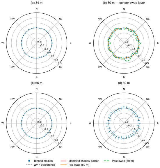
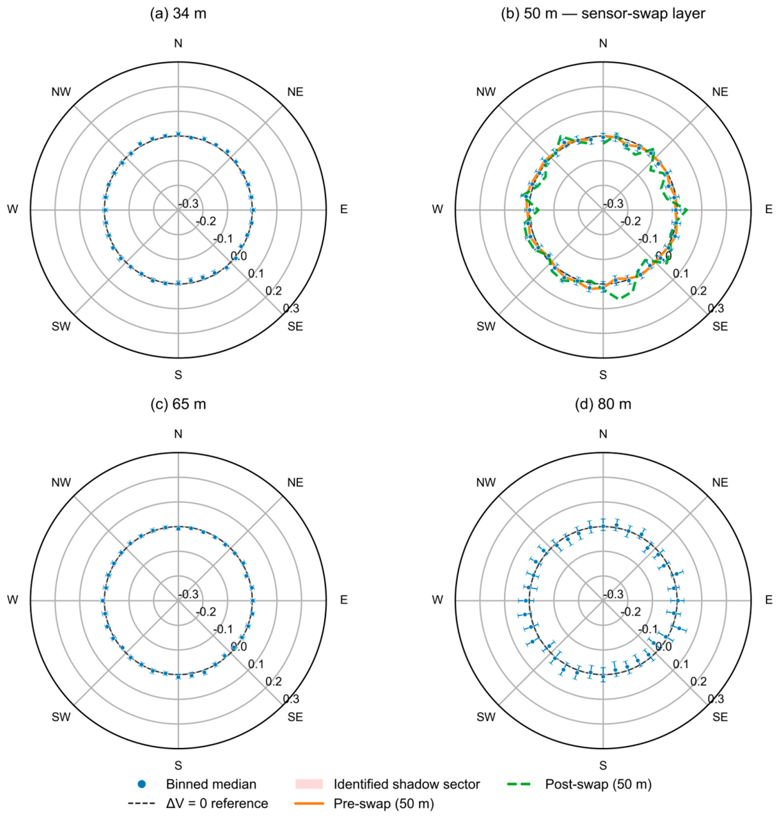
Figure 2 shows the polar-binned (10°) distribution of the east–west wind-speed difference, ΔV = V_east − V_west, as a function of the 95 m top reference wind direction for the four measurement levels. At all four levels, the median ΔV in each directional bin varies only slightly around 0 m s−1, with no systematic reduction in any sector. The block-bootstrap 95% confidence intervals for all bins include zero, and the identification algorithm does not detect any statistically significant shadow sector at 34, 50, 65, or 80 m (Figure 2a–d). The 95 m-normalized ΔV/V95 leads to the same conclusion. The confidence-interval widths do differ across levels—the 80 m error bars are the widest, reflecting stronger high-level turbulence and relatively fewer samples per bin—but the detection capability of the test is explicitly quantifiable. Using the 1 min bilateral wind-speed records (median V95 = 4.5 m s−1), the half-widths of the widest bin confidence intervals are 0.012–0.022 m s−1 across the four levels, giving MDEs of 0.024–0.043 m s−1, i.e., 0.5–1.0% of the ambient wind speed. Notably, these MDEs are all smaller than the 0.1 m s−1 resolution at which routine meteorological wind-speed observations are reported: the detection floor of the test thus lies below the scale at which wind speed is conventionally considered resolved in meteorological practice, and any sectoral deficit escaping detection is smaller than one reporting step of wind speed. Even for the shortest sub-window (the post-swap period of the 50 m level), the MDE is 0.060 m s−1, still below 0.1 m s−1. We further note that the bin medians fluctuate around zero after removal of each level’s all-direction median offset (−0.09 to +0.06 m s−1, a direction-independent inter-anemometer calibration difference within the ±2% accuracy class), with the residual direction-dependent fluctuations confined to ±0.011 m s−1.
Figure 2.
Test outcome for the tower-shadow hypothesis. (a–d) show the polar distribution of the east–west wind-speed difference ΔV = V_east − V_west against the 95 m top reference wind direction for the 34, 50, 65, and 80 m levels, respectively (10° bins; radial coordinate ΔV in m s−1, range −0.3 to +0.3). Blue dots are the bin medians, vertical error bars their block-bootstrap 95% confidence intervals, and the black dashed line the ΔV = 0 reference. In (b), the orange solid and green dashed curves are the bin-median curves for the pre- and post-swap periods of the 50 m swap level, nearly coincident. The pink marker in the legend is reserved for identified significant tower-shadow sectors. Based on the observed data, no sector is flagged at any level; that is, no significant tower shadow was detected. The larger point-to-point scatter of the post-swap (green dashed) curve in (b) reflects the ≈2.7-times smaller directional sample (1.0 yr vs. 2.7 yr per 10° bin) rather than any instrument malfunction; no sector is significant in either window.
Repeating the test for the 50 m swap level by pre- and post-swap periods, the two ΔV–wind-direction curves nearly coincide (Figure 2b), indicating that the swap event itself did not alter the level’s flow field, satisfying the DID precondition that the ambient flow field remains consistent before and after treatment. Moreover, the quantified detection floor bounds the physical relevance of any residual, undetected deficit: even a sectoral deficit at the MDE would alter shield ventilation by less than 0.1 m s−1 (about 1% of the ambient wind speed), changing the radiation-induced shield error (at most ~1 °C under low-wind, high-irradiance conditions [3,4]) by no more than ~0.01 °C—roughly two orders of magnitude below the observed 0.28–0.92 °C structural bias S(z). Undetectable tower-shadow ventilation differences are therefore physically incapable of producing the azimuthal temperature differences. In combination with the monotonic increase in the boom extension ratio L/W(z) from 0.55 at 34 m to 0.97 at 80 m (Table 1), the sensor is progressively farther from the tower with height. Thus, even if a tower-shadow mechanism were present, its influence should diminish with height. The uniformly negative result at all levels is consistent with this geometric expectation and indicates that the east–west symmetric boom design effectively eliminated detectable flow-blockage effects. Consequently, we attribute the observed east–west temperature bias to structural geometry and instrument individuality, and we reject the tower-shadow (flow-blockage) hypothesis.
3.2. Diurnal Behavior and Geometry Linkage of the Structural Baseline
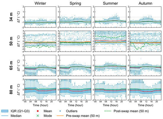
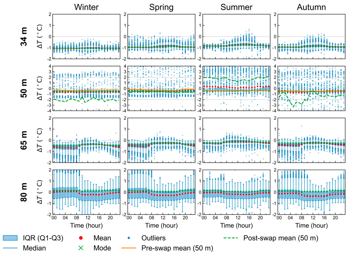
Figure 3 presents the season × hour-of-day (BJT) boxplot panorama of the east–west temperature difference ΔT = T_east − T_west across the four levels. The four rows of Figure 3 (34, 50, 65, and 80 m) are shown at enlarged scale in Figures S3, S4, S5 and S6, respectively. The three un-swapped levels remain stable throughout the year. The 34 m level maintains a median temperature near −0.9 °C in all seasons and exhibits the smallest diurnal amplitude. The 65 m level remains near −0.4 °C, with a slight afternoon increase in summer (12:00–16:00 BJT). The 80 m level consistently shows the smallest absolute temperature magnitude. In contrast, the 50 m level exhibits clear two-regime behavior: the pre-swap mean (orange solid) stays stable near −0.2 to −0.3 °C throughout the year, whereas the post-swap mean (green dashed) drops to about −2 °C in winter and rises to about +2 °C in summer, showing a pronounced seasonally dependent shift.
Figure 3.
Hourly boxplots of the east–west temperature difference ΔT = T_east − T_west, crossing the four observation levels (rows: 34/50/65/80 m) and four seasons (columns: winter/spring/summer/autumn). The box spans the interquartile range (IQR, Q1–Q3), the intra-box line is the median, red dots the mean, green crosses the mode, and whiskers extend to 1.5× IQR with outliers as scattered points. The 50 m row additionally overlays the pre-swap (orange solid) and post-swap (green dashed) hourly mean curves. The horizontal axis is hour (00–23), in BJT (UTC+8). Note that the vertical axis ranges differ by row: −4 to +4 °C for the 50 m row, −2 to +2 °C for the others.
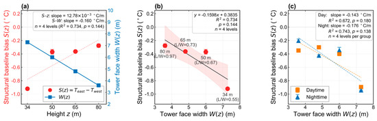
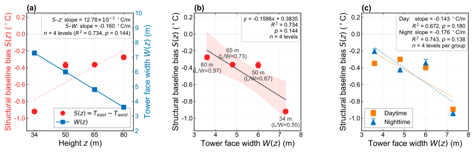
The structural baseline bias S(z), estimated over the pre-swap window, decreases monotonically in magnitude with height: from −0.92 °C at 34 m (95% CI [−0.93, −0.91]) through −0.37 °C at 50 m and −0.36 °C at 65 m to −0.28 °C at 80 m (Figure 4a, Table 2). We note that the 80 m S(z) is a mixed mean of two states before and after a spontaneous step in April–May 2024. The regression slope of S(z) against height z is +12.78 × 10⁻³ °C/m. Because tower-face width W(z) is a linear transform of height, the regression of S(z) against W(z) is numerically equivalent (Figure 4b): S(z) = −0.160·W(z) + 0.384, R2 = 0.734. Because the tower provides measurements at only four discrete vertical levels, all regressions in Figure 4 are fitted to these four independent points, and the fitted lines and confidence bands are drawn strictly within the observed W(z) range without extrapolation. We note that, limited by the n = 4 level sample size, this relationship does not reach the conventional significance level (p = 0.144), and we therefore describe it as a ‘consistent negative trend’ rather than a significant correlation.
Figure 4.
Geometry linkage and diurnal decomposition of the structural baseline bias S(z), based on the four independent observation levels of the tower. (a) S(z) (red dots with 95% CI error bars, left axis) and tower-face width W(z) (blue squares, right axis) versus height z; the height axis is ticked only at the four observation levels (34, 50, 65, 80 m, marked by dotted vertical gridlines), the blue line is the deterministic geometric function W(z) (Equation (1)), and the thin red dashed line is the de-emphasized linear trend of S(z). (b) Linear regression of S(z) on W(z): the black solid line is the fit (y = −0.1598x + 0.3835) drawn only within the observed W(z) span, the pink shaded band is the 95% regression confidence band, and each data point is labeled with its measurement level and L/W ratio; R2 = 0.734, p = 0.144, n = 4 levels, a consistent trend rather than a significant correlation. (c) Diurnal decomposition regression: orange squares and dashed line for daytime (slope −0.143 °C/m, R2 = 0.672, p = 0.180), blue triangles and dashed line for nighttime (slope −0.176 °C/m, R2 = 0.743, p = 0.138), both confined to the observed W(z) span (n = 4 levels per group); the two slopes are similar with overlapping confidence intervals, indicating a day–night stable structural effect.
Table 2.
Pre/post estimates of the structural baseline S(z) and radiative-response coefficients α/β for each level. S(z) is the pre-swap window (28 August 2022 to 11 May 2025) mean; its 95% CI is from daily-mean block bootstrap (B = 2000). α/β are Huber robust-regression slopes; Δ significance is from moving-block bootstrap (block 5 d, B = 1000).
The day–night decomposition further demonstrates the temporal stability of this structural effect (Figure 4c). The daytime regression slope is −0.143 °C/m (R2 = 0.672, p = 0.180), and the nighttime slope is −0.176 °C/m (R2 = 0.743, p = 0.138); these slopes are similar in magnitude and have overlapping confidence intervals. If S(z) were controlled by a radiative diurnal process (e.g., differential solar loading), the day and night slopes should show a clear divergence. Instead, their close agreement indicates that the underlying cause is more likely the intrinsic east–west geometric/orientation difference than a radiative dynamical process. This behavior contrasts sharply with the highly dynamic, season-sensitive bias of the 50 m level after the swap (Section 3.3).
3.3. Swap-Induced Amplification and Sign Reversal
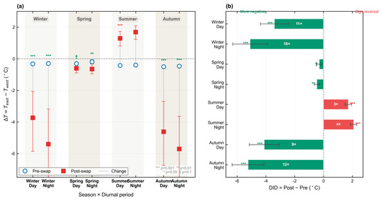
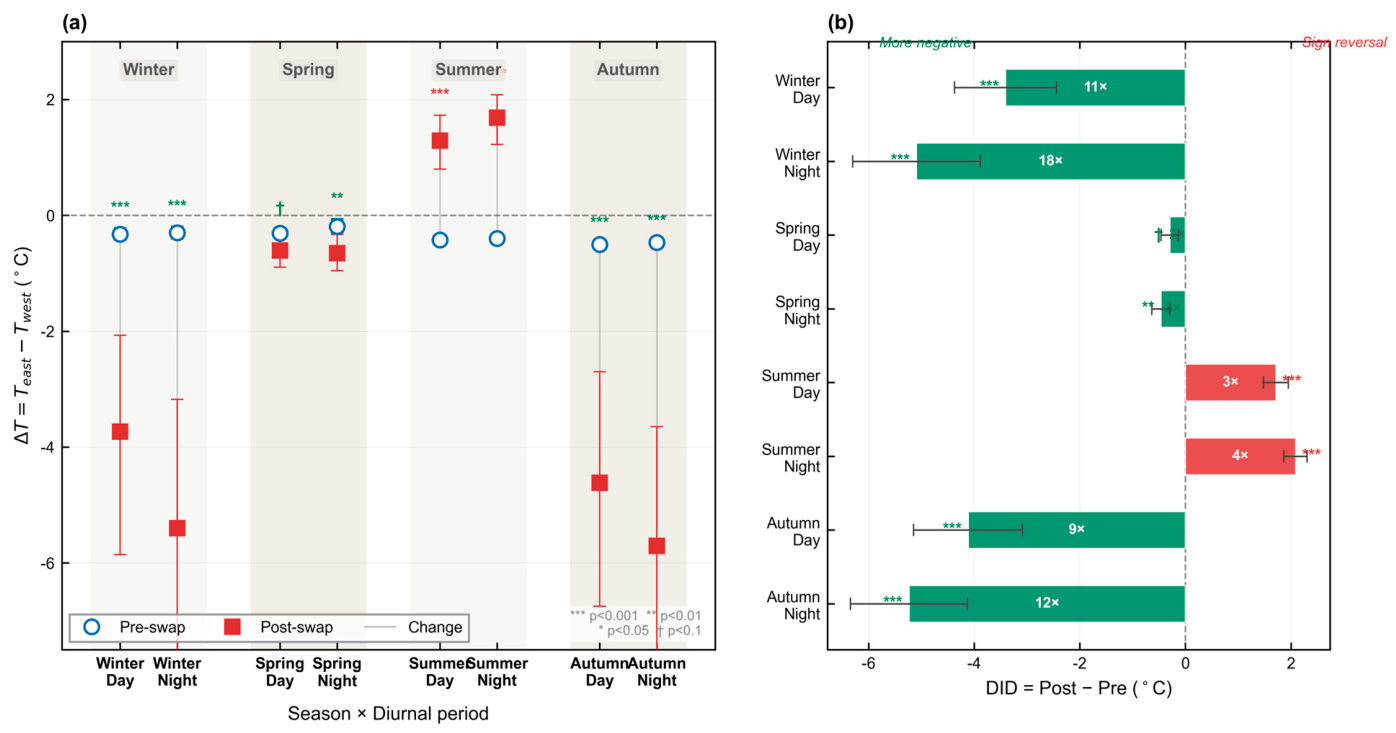
Figure 5a shows the pre-swap (blue hollow circles) and post-swap (red solid squares) group means of the 50 m ΔT across the 8 season × day–night groups. The pre-swap means vary only slightly around 0 °C (between −0.2 and −0.5 °C) with minimal differences among groups. In contrast, the post-swap means diverge markedly: winter and autumn groups shift strongly negative, summer groups become positive, and spring changes the least.
Figure 5.
Season × day–night decomposition of the 50 m swap level into 8 groups. (a) Pre-swap (blue hollow circles) and post-swap (red solid squares) ΔT means per group, gray lines connecting within-group changes, with significance stars above (*** p < 0.001, ** p < 0.01, * p < 0.05, † p < 0.1) and background bands distinguishing the four seasons. (b) Horizontal bar chart of the group DID = post − pre (°C), with black error bars as block-bootstrap 95% confidence intervals and annotations of the multiple relative to the pre-swap baseline absolute value; green bars indicate a more negative post-swap bias, red bars a sign reversal, and the gray dashed line the DID = 0 reference.
The induced effect is quantified using the within-group change DID = post − pre (Figure 5b, Table 3). For winter nights, DID = −5.10 °C, with the post-swap absolute bias reaching 18 times the pre-swap baseline; for winter days, DID = −3.41 °C (11×). For autumn nights, DID = −5.24 °C (12×), and for autumn days, DID = −4.12 °C (9×). All four cases become more negative (all p < 0.001). In contrast, both summer groups reverse sign: summer days show +1.71 °C (3×) and summer nights +2.09 °C (4×), shifting from a negative baseline to a positive bias (both p < 0.001). The two spring groups change least: spring days show −0.30 °C, only marginally significant († p < 0.1), and spring nights −0.46 °C (** p < 0.01). Negative-control checks indicate that same-group Change at the 34 and 65 m control levels fluctuates around zero (absolute value ≤ 0.06 °C) and exhibits no synchronized step analogous to that at 50 m. The 80 m level, which experienced a spontaneous ~+0.7 °C step in April–May 2024, violates the negative-control premise and is therefore excluded from the control evidence. Taken together, the negative-control analysis supports attributing the 50 m effect to the instrument rather than to a shared environmental forcing.
Table 3.
Complete results of the 8-group season × day–night DID decomposition for the 50 m level (exact script output). pre/post are window means of within-group daily means; 95% CI from block bootstrap (B = 5000); p-values from Welch t-tests on daily means; multiple = |post|/|pre|.
3.4. Pre/Post Contrasts in Radiative-Response Coefficients
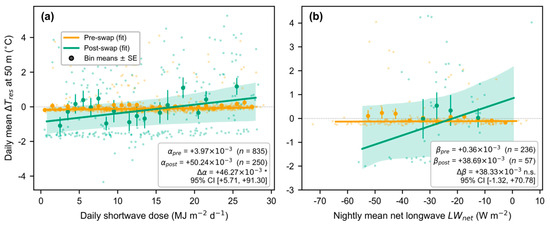
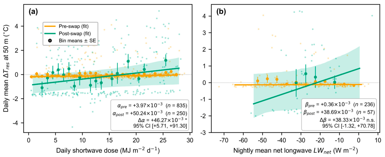
The period-centered residual ΔT_res (Equation (4)) exhibits a distinctly different radiative-forcing response before and after the instrument swap. In the daytime channel (Figure 6), the pre-swap shortwave response coefficient α_pre = +3.97 × 10⁻³ °C/(MJ m−2 d−1) is close to zero, whereas the post-swap coefficient α_post = +50.24 × 10⁻³ °C/(MJ m−2 d−1) is about 12.7 times larger. The inter-instrument difference in the shortwave response, Δα = +46.27 × 10⁻³ °C/(MJ m−2 d−1), has a 95%CI [+5.71, +91.30] that excludes zero and is therefore statistically significant. In other words, after the swap the same daily cumulative shortwave dose produces a substantially stronger temperature-difference response between the two sides. The residual ΔT_res, with the structural baseline removed, shows in the nighttime channel (Figure 6b), β_pre = +0.36 × 10⁻³ °C/(W m−2), β_post = +38.69 × 10⁻³ °C/(W m−2), and the inter-instrument difference Δβ = +38.33 × 10⁻³ °C/(W m−2) is directionally consistent with the daytime result. However, its 95% CI [−1.32, +70.78] spans zero and is therefore not statistically significant (n.s.). Notably, the nighttime DID multiples (winter night 18×, autumn night 12×) actually exceed the daytime multiples (winter day 11×, autumn day 9×), which appears inconsistent with the non-significant Δβ. Potential explanations—including limited calm-wind sampling, longwave radiation not being the sole nighttime driver, and independent contributions from instrument baseline drift—are discussed in Section 4. The regression coefficients, confidence intervals, and significance levels for both periods are summarized in Table 2. We note that both regressions are fitted to the individual daily and nightly means (daytime: n = 835/250 days; nighttime: n = 236/57 nights, pre-/post-swap), while the bin means shown in Figure 6 are visualization aids only; the per-sample explained variance of the post-swap fits is small (R2 ≈ 0.04), so the slope estimates—and the significance assessment of Δα/Δβ—rest on the moving-block bootstrap of all individual samples rather than on the binned points.
Figure 6.
Radiative-response regression results for the 50 m level. (a) Daytime channel: Huber robust regression of the daily mean ΔT_res (east–west temperature difference centered by the period mean; the pre-swap center equals the structural baseline S(z))) against the daily cumulative shortwave dose (n = 835 pre-swap days; 250 post-swap days). (b) Nighttime channel: regression of the nightly mean ΔT_res against the nightly mean net longwave radiation LW_net (positive downward, negative at night; n = 236 pre-swap nights; 57 post-swap nights). In both panels, small semi-transparent dots are the individual daily (nightly) samples to which the Huber regressions are fitted; larger circles with error bars are bin means ± standard error (1 MJ m−2 d−1 bins in (a), 5 W m−2 bins in (b); only bins containing at least 8 samples are shown); solid lines are the Huber fits, shaded bands their moving-block-bootstrap 95% confidence bands, and the gray dotted line the ΔT_res = 0 reference. The per-sample explained variance is small (post-swap R2 = 0.035 in (a) and 0.045 in (b)); in (b) the post-swap slope is anchored by the clear-sky winter nights at LW_net ≤ −40 W m−2 (ΔT_res ≈ −1 to −2 °C). Δα = +46.27 × 10⁻³ °C/(MJ m−2 d−1), 95% CI [+5.71, +91.30] (*, significant); Δβ = +38.33×10⁻³ °C/(W m−2), 95% CI [−1.32, +70.78] (n.s., directionally consistent suggestive evidence). Note that the y-axis ranges differ between the two panels. The seasonal sign reversal of the post-swap hourly mean curves at 50 m is the radiation-conditioned inter-assembly difference quantified by the regressions of Figure 6.
Internal-consistency checks show that the α and β of the 34 and 65 m control levels exhibit no significant pre/post change (both Δα and Δβ 95% CIs straddle zero, Table 2), ruling out the explanation that ‘the climatic mean state or radiation environment itself changed over the observation period.’ The 80 m level shows a significantly negative Δα (−10.68 × 10⁻³, p < 0.001), consistent with its spontaneous April–May 2024 step, and is excluded from control evidence. Only the 50 m level exhibits a significant α jump and a directionally consistent but non-significant β change, corroborating that the 50 m change is assembly-specific rather than a common environmental shift. Which physical attribute of the two assemblies differs—shield-surface aging, ventilation-port condition, or inner-wall reflectivity, candidates consistent with the sensor-to-sensor variability documented by Lefevre et al. [16]—cannot be determined from in situ differential data alone and would require paired laboratory characterization; these are therefore labeled as unconfirmed candidate mechanisms rather than findings.
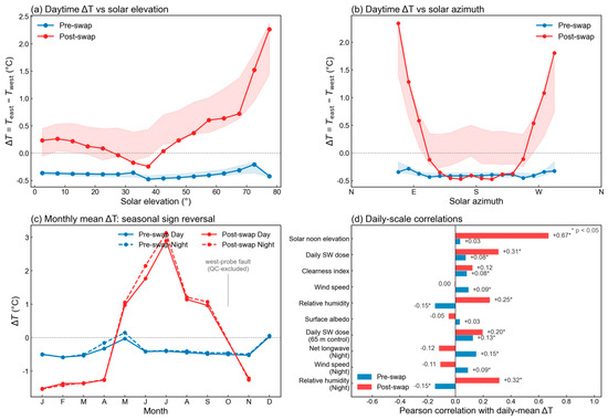
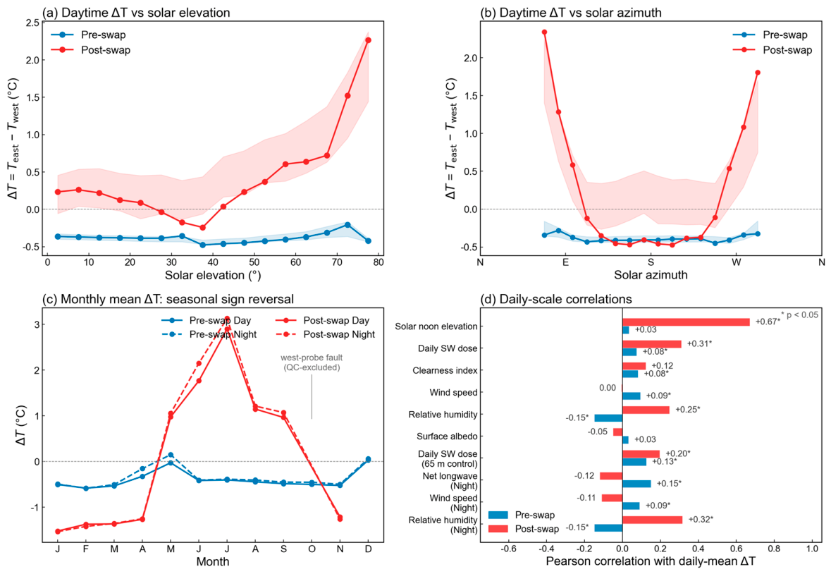
Figure 7 diagnoses the physical regime governing the seasonal reversal. Before the swap, the daytime ΔT is independent of solar geometry: the elevation- and azimuth-conditioned curves remain flat around the structural baseline (r with solar noon elevation = +0.03, n = 889 days), directly corroborating the geometric origin of the baseline. After the swap, the daily daytime ΔT correlates strongly with solar noon elevation (r = +0.67, n = 254, p < 0.001), moderately with the daily shortwave dose (r = +0.31) and relative humidity (r = +0.25), and negligibly with clearness index, wind speed, and surface albedo (|r| ≤ 0.12). Controlling for solar noon elevation, the partial correlations with dose, clearness, wind, and humidity all fall below 0.12 (not significant): the inter-instrument bias is conditioned on the background seasonal radiation regime rather than on day-to-day weather. Consistently, the elevation-conditioned curve is non-monotonic—the ~30° bin combines negative winter-midday and positive summer-morning values, i.e., the same instantaneous sun position produces opposite signs in different seasons—and the azimuth-conditioned curve is broadly symmetric between morning (+1.02 °C) and afternoon (+0.83 °C), excluding a fixed instantaneous-geometry or azimuthal origin. The 65 m control level shows only a weak correspondence (r = +0.20 after the swap), and the nighttime associations remain weak (net longwave −0.12, wind speed −0.11), consistent with the suggestive status of the nighttime mechanism; the humidity association is largely seasonal covariation (partial r = +0.12).
Figure 7.
Physical regime of the seasonal sign reversal at the 50 m level. (a) Daytime ΔT conditioned on solar elevation (5° bins; day-block-bootstrap 95% CI). (b) Daytime ΔT conditioned on solar azimuth (15° bins). (c) Monthly-mean day/night ΔT before and after the swap; the October gap reflects a west-probe fault excluded by quality control. (d) Daily-scale Pearson correlations between day/night ΔT and solar-geometry, cloudiness, ventilation, humidity, and surface-state predictors; asterisks denote p < 0.05. Blue: pre-swap; red: post-swap.
4. Discussion
In this study, we performed a controlled, full-instrument replacement on the 100 m gradient tower at the Shouxian National Climate Observatory, embedding the three candidate mechanisms—flow blockage (tower shadow), structural geometry, and inter-instrument radiative sensitivity—within a unified difference-in-differences (DID) framework for joint evaluation. The main findings are threefold. First, bilateral anemometer measurements at all four levels revealed no statistically significant shadow sector, thereby rejecting the tower-shadow hypothesis. Second, the structural baseline bias S(z) of the three un-swapped levels decreases with height and shows a consistent linear association with the height-dependent tower geometry proxied by W(z) (R2 = 0.734; n = 4, p = 0.144), stable across day and night. Third, after the swap, the 50 m bias increases to 3–18 times the baseline and exhibits a seasonal reversal, accompanied by a pronounced inter-instrument difference in the daytime shortwave response (Δα = +46.27 × 10⁻³ °C/(MJ m−2 d−1)) and a directionally consistent nighttime net longwave difference.
Existing radiation-shield error-correction approaches primarily focus on optimizing shield geometry or applying machine-learning models to improve single-point accuracy [6,7], implicitly treating the sensor as an isolated point measurement for which azimuth-induced systematic error is negligible. Our results demonstrate this assumption can be violated—the 3–18× bias amplification and pronounced seasonal sign reversal produced by the 50 m swap are difficult for conventional single-point correction models to detect or fix. As for the tower-shadow hypothesis, its negative result is directly explained by boom geometry: the boom-length-to-tower-width ratio L/W(z) increases monotonically from 0.55 at 34 m to 0.97 at 80 m. Wind-engineering studies have shown that flow distortion around lattice towers becomes negligible once the boom length exceeds roughly 0.5–0.7 times the tower width [17,20]—our tower’s lowest level (34 m, L/W = 0.55) already approaches this threshold, and the three upper levels (0.67–0.97) comfortably exceed it; moreover, the east–west booms are symmetrically placed along the tower diagonals, so that under most wind directions the two sides experience essentially identical nominal upstream conditions. It is worth noting that although the 80 m level exhibits the most favorable L/W ratio, it also presents the widest confidence interval in the ΔV analysis. This feature reflects stronger turbulence aloft and relatively limited bin samples, rather than indicating any obstruction. Moreover, the close agreement between the pre- and post-swap ΔV–wind-direction curves at 50 m (Figure 2b) further confirms that the swap did not perturb the local flow field, thereby satisfying the key DID precondition.
The absolute value of the structural baseline bias decreases with height (from −0.92 °C at 34 m to −0.28 °C at 80 m) and maintains a consistent linear relationship with W(z). Two independent lines of evidence indicate a geometric rather than radiative-dynamic origin. First, the diurnal decomposition yields nearly identical regression slopes (day −0.143 °C/m, night −0.176 °C/m, overlapping confidence intervals). If S(z) were controlled by a radiation-dependent mechanism (e.g., differential solar loading on the east–west shield surfaces), the day–night slopes would be expected to diverge systematically; instead, their temporal stability points to a persistent east–west asymmetry (background terrain, local albedo, or small geometric offsets in boom installation). We emphasize that this geometric attribution is collective rather than parameter-specific: on this tapered lattice tower, the face width W(z), the distance of each shield from the nearest structural elements, the view factor to the tower, and the effective local exposure all decrease monotonically with height and cannot be separated with n = 4 levels; W(z), available dimension-for-dimension from the construction drawings, serves as their common quantitative proxy, and the S(z)–W(z) association should therefore be read as a link to the height-dependent tower-proximity geometry as a whole rather than to the face width alone. The boom orientation itself is east–west symmetric by design (both booms along the tower diagonals) and cannot produce a signed ΔT unless the installed azimuth deviates from the drawing (limitation (5)). Second, this stable baseline contrasts sharply with the highly dynamic, season-sensitive behavior of the 50 m level after the swap—the stable geometric driver and the dynamic instrument driver operate on different time scales and can be empirically separated by the controlled-swap design. This constitutes, beyond rejecting the tower-shadow hypothesis, our second methodological contribution.
The pronounced daytime shortwave-response difference (Δα = +46.27 × 10⁻³ °C/(MJ m−2 d−1), 95% CI [+5.71, +91.30]) provides direct evidence for an inter-instrument discrepancy in shortwave radiative-response sensitivity. This finding is consistent with Lefevre et al. [16], who reported substantial sensor-to-sensor variability in shield errors and attributed it to shield-surface aging, dust accumulation in ventilation ports, and reduced inner-wall reflectivity. The nighttime result presents an apparent paradox: the nighttime DID multiple (winter night 18×, autumn night 12×) exceeds the corresponding daytime values (winter day 11×, autumn day 9×), yet the nighttime net-longwave difference Δβ = +38.33 × 10⁻³ °C/(W m−2) is not statistically significant (95% CI [−1.32, +70.78]). We consider three non-mutually-exclusive explanations. First, the calm-wind screening (wind speed < 1.5 m/s) substantially reduces the nighttime sample size, thereby weakening statistical power. Second, net longwave radiation may not be the only nighttime driver of the azimuthal temperature difference; residual turbulent mixing and instrument baseline drift can introduce additional variance. Third, if the two shields differ in longwave emissivity, the resulting differential radiative cooling may manifest primarily as an approximately constant offset rather than a change in slope, placing it outside the detection capability of our regression framework. A sensitivity analysis that lowers the calm-wind threshold to 1.5 m/s yields a consistent result (Δβ = +50.97 × 10⁻³ °C/(W m−2), p = 0.16), indicating that the qualitative assessment is robust to the choice of threshold. We therefore characterize the nighttime evidence as ‘directionally consistent suggestive evidence’: the nighttime DID multiple is large but cannot yet be fully accounted for by Δβ alone.
These findings carry direct implications for homogenization practice in climate observing networks. Homogenization algorithms typically detect and correct temperature-series steps induced by instrument changes [28,30], resting on the core assumption that a step corresponds to an approximately constant offset [29,31]. Our swap, however, induces a bias that is anything but constant—its magnitude ranges from −5.10 °C on winter nights to +2.09 °C on summer nights, a seasonal amplitude exceeding 7 °C with sign reversal (Table 3)—so that a single-offset correction would systematically over-correct winter months and under-correct summer months. Meanwhile, the significance of Δα indicates that the bias magnitude depends on incident radiative forcing, so that the same instrument pair can produce different apparent offsets under different radiation environments. We therefore recommend that, where conditions permit, homogenization procedures evaluate step changes as a function of environmental covariates (e.g., solar radiation, wind speed) [28,30], and that station-network metadata record not only instrument-change dates but, where possible, the radiative-response characterization of the paired sensors.
Beyond network homogenization, our audit yields five transferable signatures that other tower-based experiments can watch for after any positional exchange of sensor assemblies: (i) a radiation-conditioned, seasonally reversing ΔT rather than a fixed step change; (ii) a significant change in the regression slope of ΔT against the daily shortwave dose (α contrast); (iii) amplified nighttime ΔT under calm winds, directionally consistent with net-longwave loss; (iv) unchanged bilateral ΔV–wind-direction statistics, confirming flow-field stability and the DID precondition; and (v) the absence of synchronized steps at un-swapped control levels, excluding environmental causes. Where operationally possible, we recommend scheduling paired laboratory characterization of both assemblies around the exchange and a subsequent swap-back test.
This study has several limitations that should be acknowledged. (1) Spatial representativeness: single-tower observations cannot be directly generalized to stations with different tower geometries, boom configurations, or climatic conditions [32]; the S(z)–W(z) relation awaits validation at other sites. (2) Radiation proxy: shortwave and longwave radiation are taken from station-level single-point observations, which neglects the vertical gradient of radiation (e.g., fog, low cloud, or vegetation-canopy effects), which is especially pronounced for the lowest level (34 m). (3) Post-swap duration: the post-swap period is about one year, covering only a single complete seasonal cycle. (4) Statistical power: the S(z)–W(z) regression rests on n = 4 levels and cannot support a formal significance test. (5) Boom magnetic azimuth: the precise magnetic azimuth of each boom (the construction drawing only notes ‘along the tower diagonal’) has not been verified with an on-site compass, and small deviations from true east–west may contribute to the structural baseline. Relatedly, the geometric parameters plausibly governing S(z)—face width, shield-to-structure distance, tower view factor, and local exposure—co-vary monotonically with height on the tapered tower and cannot be disentangled at n = 4 levels; the S(z)–W(z) association therefore identifies the height-dependent tower-proximity geometry collectively, and separating the individual parameters would require dedicated numerical simulation (e.g., CFD) or targeted field measurements. (6) Control-level non-stationarity: the 80 m level exhibited a spontaneous ~+0.7 °C step in April–May 2024, plausibly an unrecorded instrument maintenance or drift, whose maintenance log is still being verified; its S(z) is a mixed mean of two states and its α also differs significantly pre/post, so the negative-control evidence comes only from the 34 and 65 m levels. This event does not affect the validity of the 50 m conclusion—the 50 m step corresponds strictly in time to the controlled swap event, and its magnitude (3–18×) far exceeds the 80 m drift. (7) No physical inspection of the swapped assemblies: after the swap, the two 50 m assemblies were not removed for laboratory examination, constrained by the continuous-operation requirements of the observatory. The audit therefore quantifies the inter-assembly difference without attributing it to a specific unit or physical attribute. A future swap-back test cannot be assumed to restore the pre-swap baseline if the cause is progressive (e.g., shield aging); the decisive protocol for future audits is paired laboratory characterization (shield reflectivity and ventilation inspection) of both assemblies scheduled around the exchange, together with a swap-back test where operationally possible. The above limitations do not affect the core finding—the tower-shadow rejection is robust at all four levels, and the swap-induced bias magnitude far exceeds what azimuthal uncertainty can explain—but they constrain the precision of quantitative generalization. (8) Calibration floor: the upper-level baselines (|S(65 m)| = 0.36 °C, |S(80 m)| = 0.28 °C) are comparable to the ±0.24 °C root-sum-square inter-probe calibration envelope, so their absolute magnitudes should be interpreted within this floor; all swap-contrast conclusions are unaffected (Section 2.1).
5. Conclusions
We integrated the three candidate mechanisms—flow blockage, structural geometry, and inter-instrument radiative sensitivity—into a unified DID experimental framework to enable joint testing and clear separation of their effects. Specifically, the flow-blockage hypothesis is rejected based on the combined evidence from independent bilateral anemometry and the top reference wind direction; the structural baseline bias exhibits a consistent geometric association with tower-face width and remains stable between day and night, indicating a geometric/orientation origin; the 3–18× amplification and seasonal sign reversal revealed by the full-instrument swap are quantified in daytime as a significant inter-instrument difference in shortwave radiative-response sensitivity, with the underlying physical attribute of the assemblies remaining to be identified by laboratory characterization, while the nighttime evidence remains directionally consistent but not significant; the 34 and 65 m control levels show no synchronized step at any time, supporting an instrument-based attribution. The homogeneity break associated with the instrument change is essentially a radiation-conditioned dynamic bias rather than a fixed offset, providing a mechanistic foundation for climate-network homogenization and azimuthal quality control on tower-mounted systems. Future work should validate the S(z)–W(z) relation at additional levels and on towers with different geometries, verify boom magnetic azimuths in situ, and develop a multidriver decomposition framework for nighttime azimuthal bias.
Supplementary Materials
The following supporting information can be downloaded at: https://www.mdpi.com/article/10.3390/app162010025/s1, Figure S1: station location, full-resolution version of Figure 1a; Figure S2: tower general arrangement, full-resolution version of Figure 1c; Figures S3–S6: enlarged single-level versions of the 34, 50, 65, and 80 m rows of Figure 3.
Author Contributions
Conceptualization, L.C. and X.L.; methodology, L.C. and X.L.; software, L.C.; validation, L.C., C.D. and K.Z.; formal analysis, L.C.; investigation, L.C., C.D., K.Z., H.Z., C.Z. and Y.L.; resources, X.L., C.D. and H.Z.; data curation, L.C., K.Z. and H.Z.; writing—original draft preparation, L.C.; writing—review and editing, X.L., C.D., K.Z., H.Z., C.Z. and Y.L.; visualization, L.C.; supervision, X.L.; project administration, X.L.; funding acquisition, X.L. All authors have read and agreed to the published version of the manuscript.
Funding
This research was funded by the Anhui Provincial Natural Science Foundation (Grant No.2408055UQ001) and the Anhui Meteorological Bureau (Innovation and Development Special Project, grant number CXQ202504).
Institutional Review Board Statement
Not applicable.
Informed Consent Statement
Not applicable.
Data Availability Statement
The data presented in this study are available on request from the corresponding author.
Acknowledgments
The authors would like to thank the Shouxian National Climate Observatory for providing all the meteorological observational data used in this study. We are also grateful to the observatory’s staff for their sustained efforts in operating and maintaining the 100 m gradient observation tower, which made this work possible. During the preparation of this manuscript, the authors used Kimi (Moonshot AI, version K3; https://kimi.moonshot.cn) for the purposes of programming the data processing and figure generation and for AI-assisted translation of the manuscript from Chinese to English. The authors have reviewed and edited the output and take full responsibility for the content of this publication.
Conflicts of Interest
The authors declare no conflicts of interest.
Abbreviations
The following abbreviations are used in this manuscript:
| BJT | Beijing time (UTC+8) |
| CFD | computational fluid dynamics |
| DID | difference-in-differences |
| IQR | interquartile range |
| WMO | World Meteorological Organization |
References
- Nakamura, R.; Mahrt, L. Air Temperature Measurement Errors in Naturally Ventilated Radiation Shields. J. Atmos. Ocean. Technol. 2005, 22, 1046–1058. [Google Scholar] [CrossRef] [Scilit]
- Lin, X.; Hubbard, K.G.; Walter-Shea, E.A. Radiation loading model for evaluating air temperature errors with a non-aspirated radiation shield. Trans. ASAE 2001, 44, 1299. [Google Scholar] [CrossRef] [Scilit]
- Lin, X.; Hubbard, K.G.; Walter-Shea, E.A.; Brandle, J.R.; Meyer, G.E. Some Perspectives on Recent In Situ Air Temperature Observations: Modeling the Microclimate inside the Radiation Shields*. J. Atmos. Ocean. Technol. 2001, 18, 1470–1484. [Google Scholar] [CrossRef] [Scilit]
- Richardson, S.J. Multiplate Radiation Shields: Investigating Radiational Heating Errors. Ph.D. Thesis, The University of Oklahoma, Norman, OK, USA, 1995. Available online: https://search.proquest.com/openview/36c2cc8caa7be4b29a8a8b2ebbe60f50/1 (accessed on 15 June 2026).
- Nakamura, R.; Mahrt, L. Air temperature measurement errors in a naturally ventilated multi-plate radiation shield. In Proceedings of the 16th Symposium on Boundary Layers and Turbulence, Portland, ME, USA, 9–13 August 2004; Available online: https://www.researchgate.net/publication/237296536 (accessed on 15 June 2026).
- Jin, W.; Liu, Q.; Dai, W.; Hong, X.; Cao, X.; Sun, H. Optimized Design and Radiation Error Correction of a Naturally Ventilated Air Temperature Sensor for Atmospheric Environmental Monitoring. Sensors 2026, 26, 3853. [Google Scholar] [CrossRef] [Scilit] [PubMed]
- Li, L.; Yuan, K.; Chen, Y. Development of an Air Temperature Observation System Using a Radiation Shield and Neural Network Correction. Sensors 2026, 26, 3715. [Google Scholar] [CrossRef] [Scilit] [PubMed]
- Sakalis, V.D. A New Empirical Method for Correction of Daytime Air Temperature Measurement Errors in Naturally Ventilated Radiation Shields. Bull. Atmos. Sci. Technol. 2022, 3, 9. [Google Scholar] [CrossRef] [Scilit]
- Yang, J.; Liu, Q.; Dai, W.; Ding, R. A Temperature Error Correction Method for a Naturally Ventilated Radiation Shield. J. Atmos. Sol.-Terr. Phys. 2016, 149, 40–45. [Google Scholar] [CrossRef] [Scilit]
- Yang, J.; Liu, Q.; Dai, W. A temperature error correction method for a DTR503A naturally ventilated radiation shield. Heat Transf. Res. 2017, 48, 1421–1432. [Google Scholar] [CrossRef] [Scilit]
- Yang, J.; Deng, X.; Liu, Q.; Ding, R. Design and Experimental Study of an Effective, Low-Cost, Naturally Ventilated Radiation Shield for Monitoring Surface Air Temperature. Meteorol. Atmos. Phys. 2021, 133, 349–357. [Google Scholar] [CrossRef] [Scilit]
- Jin, W.; Zhou, Y.; Tang, J.; Amdadul, H.M. Design and Experimental Validation of a High-Accuracy Naturally Ventilated Radiation Shield for Near-Surface Air Temperature Observation. Atmosphere 2026, 17, 272. [Google Scholar] [CrossRef] [Scilit]
- Liu, Q.; Jin, W.; Yang, J.; Zhu, H.; Dai, W. Design and Experiments of a Naturally-Ventilated Radiation Shield for Ground Temperature Measurement. Atmosphere 2023, 14, 523. [Google Scholar] [CrossRef] [Scilit]
- Sun, X.; Yan, S.; Wang, B.; Xia, L.; Liu, Q.; Zhang, H. Air Temperature Error Correction Based on Solar Radiation in an Economical Meteorological Wireless Sensor Network. Sensors 2015, 15, 18114–18139. [Google Scholar] [CrossRef] [Scilit] [PubMed]
- Wang, B.; Gu, X.; Yan, S. STCS: A Practical Solar Radiation Based Temperature Correction Scheme in Meteorological WSN. Int. J. Sens. Netw. 2018, 28, 22. [Google Scholar] [CrossRef] [Scilit]
- Lefevre, A.; Malet-Damour, B.; Rivière, G. Development of a Metrological Framework Based on Irradiance and Ventilation for the Characterization and Correction of Low-Cost Radiation Shield Errors. Metrology 2026, 6, 50. [Google Scholar] [CrossRef] [Scilit]
- Orlando, S.; Bale, A.; Johnson, D.A. Experimental Study of the Effect of Tower Shadow on Anemometer Readings. J. Wind Eng. Ind. Aerodyn. 2011, 99, 1–6. [Google Scholar] [CrossRef] [Scilit]
- Lubitz, W.D.; Michalak, A. Experimental and Theoretical Investigation of Tower Shadow Impacts on Anemometer Measurements. J. Wind Eng. Ind. Aerodyn. 2018, 176, 112–119. [Google Scholar] [CrossRef] [Scilit]
- Lubitz, W.D. Effects of tower shadowing on anemometer data. In Proceedings of the 11th Americas Conference on Wind Engineering, San Juan, PR, USA, 22–26 June 2009; Available online: https://www.researchgate.net/publication/259757827_Effects_of_Tower_Shadowing_on_Anemometer_Data (accessed on 15 June 2026).
- Farrugia, R.N.; Sant, T. Wind Speed Measurements in the Vicinity of a Tubular Mast: Influence of Data Selection Methods on Wind Speed Average Determination. Wind Eng. 2014, 38, 147–166. [Google Scholar] [CrossRef] [Scilit]
- Farrugia, R.N.; Sant, T. Modelling Wind Speeds for Cup Anemometers Mounted on Opposite Sides of a Lattice Tower: A Case Study. J. Wind Eng. Ind. Aerodyn. 2013, 115, 173–183. [Google Scholar] [CrossRef] [Scilit]
- Wyngaard, J.C. Flow-Distortion Effects on Scalar Flux Measurements in the Surface Layer: Implications for Sensor Design. Bound.-Layer Meteorol. 1988, 42, 19–26. [Google Scholar] [CrossRef] [Scilit]
- McCaffrey, K.; Quelet, P.T.; Choukulkar, A.; Wilczak, J.M.; Wolfe, D.E.; Oncley, S.P.; Brewer, W.A.; Debnath, M.; Ashton, R.; Iungo, G.V.; et al. Identification of Tower-Wake Distortions Using Sonic Anemometer and Lidar Measurements. Atmos. Meas. Tech. 2017, 10, 393–407. [Google Scholar] [CrossRef] [Scilit]
- Stuurman, J.J. Automating Air Temperature Siting Classification of Meteorological Stations According to the World Meteorological Organization Guidelines. Master’s Thesis, Utrecht University, Utrecht, The Netherlands, 2019. Available online: https://studenttheses.uu.nl/bitstream/handle/20.500.12932/32845/ (accessed on 15 June 2026).
- GB 50009-2001; Load Code for the Design of Building Structures. China Architecture & Building Press: Beijing, China, 2002.
- GB 50011-2001; Code for Seismic Design of Buildings. China Architecture & Building Press: Beijing, China, 2001.
- ISO 9060:2018; Solar Energy—Specification and Classification of Instruments for Measuring Hemispherical Solar and Direct Solar Radiation. ISO: Geneva, Switzerland, 2018.
- Kaspar, F.; Hannak, L.; Schreiber, K.-J. Climate Reference Stations in Germany: Status, Parallel Measurements and Homogeneity of Temperature Time Series. Adv. Sci. Res. 2016, 13, 163–171. [Google Scholar] [CrossRef] [Scilit][Green Version]
- Menne, M.J.; Williams, C.N. Homogenization of Temperature Series via Pairwise Comparisons. J. Clim. 2009, 22, 1700–1717. [Google Scholar] [CrossRef] [Scilit]
- Hannak, L.; Friedrich, K.; Imbery, F.; Kaspar, F. Analyzing the Impact of Automatization Using Parallel Daily Mean Temperature Series Including Breakpoint Detection and Homogenization. Int. J. Climatol. 2020, 40, 6544–6559. [Google Scholar] [CrossRef] [Scilit]
- Domonkos, P.; Tóth, R.; Nyitrai, L. Data Quality Control and Dataset Development. In Climate Observations; Elsevier: Amsterdam, The Netherlands, 2023; pp. 59–81. [Google Scholar]
- Steinfeld, G.; Letzel, M.O.; Raasch, S.; Kanda, M.; Inagaki, A. Spatial Representativeness of Single Tower Measurements and the Imbalance Problem with Eddy-Covariance Fluxes: Results of a Large-Eddy Simulation Study. Bound.-Layer Meteorol. 2007, 123, 77–98. [Google Scholar] [CrossRef] [Scilit]

Disclaimer/Publisher’s Note: The statements, opinions and data contained in all publications are solely those of the individual author(s) and contributor(s) and not of MDPI and/or the editor(s). MDPI and/or the editor(s) disclaim responsibility for any injury to people or property resulting from any ideas, methods, instructions or products referred to in the content. |
© 2026 by the authors. Licensee MDPI, Basel, Switzerland. This article is an open access article distributed under the terms and conditions of the Creative Commons Attribution (CC BY) license.