


Abstract
Tidal influence is a well-known phenomenon in the hydrogeology of coastal areas, as it is transmitted through aquifers connected to the sea, generating periodic fluctuations in borehole piezometric levels. The analysis of these fluctuations makes it possible to assess subsurface properties and derive characteristic parameters from the transmission of the pressure wave. Tidal influence results from a complex combination of the gravitational attraction exerted by the Sun and the Moon on the oceanic water mass, the tidal distribution conditioned by ocean morphology, and variable meteorological effects that may be highly localised. The combination of these factors generates oscillations ranging in magnitude from metres to centimetres. Under certain circumstances, such as spring tides coinciding with low atmospheric pressure, these oscillations may cause flooding and other undesirable effects in sensitive areas. The effect of earth tides in inland areas disconnected from the sea, sometimes at high elevations, is also well known and has received increasing scientific attention. Tidal oscillations, which are readily apparent in coastal areas, can also be recorded in certain geological materials, producing fluctuations that can be detected using high-precision sensors. These oscillations are caused by the same gravitational attraction responsible for ocean tides; however, in this case, the gravitational forcing acts on the geological formation itself, giving rise to what is known as an Earth tide or astronomical tide. Recent technological advances have facilitated the detection of these phenomena, which were previously difficult to identify. This study analyses the astronomical influence detected in areas clearly isolated from the sea, focusing on small, low-permeability aquifers where direct gravitational forcing of the groundwater mass cannot account for the observed response. Instead, astronomical forcing acts on the rock mass and indirectly affects piezometric levels. The selected experimental site comprises variable lithologies and different degrees of aquifer confinement and includes numerous research boreholes. It therefore provides an optimal setting for analysing the relationship between lithology and astronomical influence and may serve as a basis for future research in different hydrogeological settings.
1. Introduction
The hydrogeological characterisation of the subsurface environment hinges on two critical aspects that have been the focus of research and countless studies throughout history. The first is the analysis of aquifer recharge, which is intrinsically linked to rain-water infiltration and acts as the primary water source in aquifers. The second involves the determination and understanding of key hydrodynamic parameters, particularly transmissivity (T) and permeability (K), which govern an aquifer’s capacity to transmit water, as well as effective porosity (me) and the storage coefficient (S), which define its water storage potential. The determination of these parameters is essential for ground-water interaction studies, including civil engineering projects, pollution control, and, more recently, the analysis of long-term data to evaluate climate change impacts on groundwater systems. Modern mathematical simulation techniques demand both accurate characteristic parameters and extensive time series data for evaluating past and future scenarios.
Classically, the hydrodynamic parameters of an aquifer are obtained by direct methods based on pumping tests [1,2,3,4], which require the execution of pumping wells, observation piezometers, and pumps. In civil works, the determination of parameters is carried out on an ad hoc basis by means of Slug Tests, Lefranc Tests, and/or Lugeon Tests [5], which are tests that are standardised [6,7,8,9] and have a validity limited to the areas where they are carried out, so they should never be extrapolated to a complete aquifer. Since pumping tests are costly, researchers have long explored indirect methods to determine these parameters, primarily through monitoring water levels (surface and groundwater) and spring flows, including the analysis of depletion coefficients, recession curves, and recharge processes.
This article focuses particularly on the analysis of tidal influence, specifically Earth tides, whose most evident effects occur in the sea but which, as will be shown, also affect groundwater in certain types of inland aquifers, i.e., aquifers with no possible connection to the sea. In oceanography, the harmonic constituents associated with gravitational dynamics resulting from the interaction of the Earth–Sun–Moon system are well known. Analysis of these constituents makes it possible to predict tidal motion, which is essential in coastal areas.
The first harmonic model of the Earth–Sun–Moon system was proposed by Thompson (Lord Kelvin, 1882) [10] and was subsequently developed in depth by the astronomer George Howard Darwin (1901) [11], son of the renowned naturalist Charles Darwin. Darwin introduced a nomenclature for harmonic motions (Darwinian Names), and Doodson (1921) [12] later characterised and parameterised harmonic motions using as many as 400 constituents, thereby establishing a basis for tidal analysis and prediction during the twentieth century.
In simplified terms, the harmonic constituents can be divided into three basic types according to their frequency:
- Diurnal constituents (1 cycle per day): These occur once per day. The mainconstituents are as follows:
- a.
- O1: Principal lunar diurnalconstituent (25.82 h).
- b.
- P1: Principal solar diurnal constituent (24.07 h).
- c.
- K1: Lunisolar diurnal constituent resulting from the interaction between the Moon and the Sun (23.93 h).
- Semidiurnal constituents (2 cycles per day): These exhibit approximately two phases per day. The mainconstituents are as follows:
- a.
- M2: Principal lunar semidiurnal constituent. It is the most important constituent (12.42 h).
- b.
- S2: Principal solar semidiurnal constituent. It is less important than M2 (12 h).
- c.
- N2: Elliptic lunar semidiurnal constituent resulting from variations in the Moon’s orbital distance (elliptical orbit, 12.66 h).
- d.
- K2: Constituent associated with changes in the declination of the Sun and the Moon (11.97 h).
- Long-period constituents: These have periods longer than 1 day. The main constituents are as follows:
- a.
- Mf: Principal lunar fortnightly constituent.
- b.
- Mm: Principal lunar monthlyconstituent.
As shown in Table 1, the main constituents are the principal lunar semidiurnal (M2), principal solar semidiurnal (S2), lunisolar diurnal (K1), and principal lunar diurnal (O1) constituents, which together account for more than 95% of the free-surface oscillation in the open sea. It is important to note that the largest tides do not reach their maximum response when the Moon and/or the Sun are directly above the observation point, but rather through their effect on the ocean, where a complex tidal distribution system develops in which tides rotate around amphidromic points (points at which the tidal amplitude is zero). From these points, cotidal lines (lines joining locations where high tide occurs at the same time) and corange lines (lines joining locations with the same difference between high and low tide) are defined. In the following figure (Figure 1), an observation point at a port on the northern coast of Spain (Bilbao) was selected, and the evolution of the tide observed every 5 min was analysed together with the positions of the Moon and the Sun relative to the observation point. A relevant feature from a hydrogeological perspective can be observed: during spring tides, there is a marked difference between the daily tidal maxima associated with the semidiurnal constituent cycle.
Table 1.
Main harmonic constituents in tidal dynamics.
Figure 1.
Evolution of the tide observed every 5 min between 10 and 25 March 2026 and positions of the Sun and Moon relative to the observation point (red circle): (a) positions during neap-tide periods, when the S2 constituent interferes with M2, and during spring tides, when both constituents reinforce each other, whether the Sun and Moon are above the observation point or on the opposite side of the Earth; (b) lunar phases between neap and spring tides, indicating the position of the Sun relative to the Moon and the observation point; (c) detail of the differences observed between the daily maxima, particularly noticeable during spring tides and associated with the way in which the attraction of the solar and lunar constituents acts.
This complex interaction between gravitational forces produces a resulting harmonic motion that is also influenced by barometric pressure. The tidal signal is therefore separated into two components: an astronomical component and a meteorological or barometric component.
This influence is transmitted to aquifers, either in coastal areas where they are directly connected to the sea or in inland areas where large water bodies are present or where geological materials exhibit a certain degree of “elasticity” in response to gravitational forcing. For this reason, numerous authors use this phenomenon to analyse aquifers by means of indirect techniques of this type.
One of the earliest authors to report tidal influence in aquifers was Meinzer (1939) [13], who analysed possible causes of water-level fluctuations. As early as 1939, he noted fluctuations associated with barometric pressure, earthquakes, ocean and Earth tides, and, for example, railway traffic, all of which had become detectable through the use of new continuous-recording systems (hydrographs). He presented the example of a 270ft (61m) well near Carlsbad, New Mexico, located 500 miles from the coast, in which semidiurnal fluctuations on the order of 0.05 ft (1.52 cm) could be observed.
Research on tidal influence was originally developed from the analysis of water levels in aquifers subjected to direct tidal forcing. These aquifers exhibit periodic oscillations in which attenuation of the tidal-wave amplitude and a phase shift or time lag can be detected and related to the hydrodynamic parameters of the aquifer, specifically transmissivity (T) and the storage coefficient (S). The first author to develop this analytical technique was Ferris [14] in 1951, although he studied confined aquifers on the basis of wave theory applied to flow in a confined porous medium, as developed by Theis (1935) [1] and subsequently adapted to semi-confined media by Jacob (1946) [2] and Hantush and Jacob (1955) [3]. Ferris established methods for determining what is known as aquifer diffusivity [4], i.e., the ratio of transmissivity to the storage coefficient (L2T−1).
Subsequently, other researchers analysed and further developed the technique initiated by Ferris, including Carr and Van der Kamp (1969) [15], Erskine (1991) [16], Pandit, El-Khazen and Sivaramapillai (1991) [17], Crowe (1994) [18], and White and Roberts (1994) [19].
Detailed analyses of the Ferris method can be found in Carrington (1995) [20,21], while the determination of diffusivity is discussed in Pinder et al. (1969) [22]. Numerous examples of applications to coastal aquifers are provided in [23,24,25,26,27]. Further information on groundwater fluctuations can also be found in [4,28,29,30].
In these cases, the piezometric wave generated in a borehole by the passage of a tidal wave through a permeable medium depends on the properties of that medium. Consequently, analysis of this wave transmission makes it possible to obtain key hydrodynamic parameters for aquifer characterisation. These parameters can be used in mathematical simulations to reproduce aquifer responses under different scenarios, such as climate-change scenarios or prolonged droughts. Such simulations must be calibrated against observational data, which requires continuous monitoring over extended periods.
Studies of tidal influence are currently being extended to inland aquifers with no connection to the sea, where periodic oscillations, generally of smaller amplitude, are also observed. In these settings, the influence (astronomical forcing in this case) does not act directly on the groundwater; instead, it acts on the geological medium, causing elastic deformation that is transmitted to the water. Numerous authors are therefore developing methods to determine the poroelastic properties of geological materials and, from piezometric oscillations, infer the geomechanical and hydrogeological characteristics of the subsurface, as well as numerically simulate the process. These approaches are based on Biot (1941) [31], who developed the laws governing consolidation when a geological medium is subjected to pressure, producing an elastic response in a porous medium that is related to changes in pore pressure. Bredehoeft (1967) [32] analysed and developed models aimed at determining aquifer specific storage inferred from tidal oscillations, although some controversy arose regarding the drained versus undrained behaviour of the porous medium, a topic reviewed by Hsieh et al. (1988) [33]. Numerous authors subsequently began to analyse Earth-tide effects in different types of media, including unconfined or partially confined aquifers, as in Maréchal et al. (2010) [34], and crystalline rock masses, as in Rojstaczer (1990) [35]. Mathematical models incorporating the elastic properties of the geological medium are currently being developed, as in Wang et al. (2018) [36] and Bastias et al. (2022) [37]. Of particular relevance is the study by Allégre et al. (2016) [38], which analysed Earth tides in an area of California with characteristics similar to those of the present study in order to obtain permeability values and compare them with values derived from field tests.
The objective of the present study is to demonstrate and corroborate, using real examples, that the analysis of wave transmission through a permeable medium is not limited to classical techniques applied in coastal environments. Owing to the use of high-precision instruments, similar wave phenomena can be observed in detail in settings unrelated to the sea or to large bodies of water. These phenomena result from poroelastic deformation of the rock mass caused by the gravitational attraction of the Sun and the Moon acting on the ground (Earth tides). This deformation, in turn, affects the water contained within the pores (pore pressure), producing an indirect piezometric response that is recorded by the aforementioned high-precision instruments installed in boreholes (observation piezometers) intersecting geological materials with different geological and hydrogeological characteristics.
2. Geological and Hydrogeological Context
2.1. LocalGeology
A study area located far from the sea was selected at a distance of more than 60 km and at elevations above 900 masl. The research area is located in the province of Palencia (Spain), in a zone characterised by major tectonic structures generally associated with thrust faults with décollement horizons in Triassic materials. As a result, the Jurassic materials are deformed, fractured, and tilted. Cretaceous materials were deposited unconformably over the Jurassic units. Consequently, the Jurassic materials exhibit steep dips, whereas the Cretaceous materials show very gentle dips (Figure 2).
Figure 2.
Location of the research area within its geological setting (MAGNA geological mapping by IGME [39]).
The research area focuses particularly on Jurassic materials, which dip eastward at angles ranging from 30° to 60°. The Jurassic sequence is crossed by a major reverse fault that places Middle Jurassic (Dogger) materials over Upper Jurassic (Malm) materials. Consequently, marine limestones predominate on the western slope, whereas continental-origin materials, including lacustrine limestones, sandstones, and marls, coexist in the upper part of the area and on the eastern slope (Figure 3).
Figure 3.
Marker beds at the surface (white), faults (red), and W–E interpretative cross-section based on borehole data.
The arrangement and diverse nature of these materials allow two small aquifers with clearly differentiated behaviour to coexist (Figure 4):
Figure 4.
Observed levels in boreholes tapping the lower aquifer (blue), which shows a rapid response, and the upper aquifer (green), which shows an attenuated response.
- On the one hand, a lower aquifer (Dogger) exhibits a relatively rapid response to recharge, with deeper groundwater levels in a predominantly carbonate medium where recharge occurs from the ground surface through preferential flow within the carbonate materials.
- On the other hand, an upper multilayer aquifer (Malm) shows clear limitations to recharge because clayey and marly low-permeability layers semi-confine the more permeable intervals. Piezometric levels are shallow and show only a limited response to recharge. Farther east, these materials become confined beneath clayey deposits, while sandy and marly materials become less abundant, resulting in a transition from a semi-confined to a confined setting.
A hydrogeologically relevant aspect is that in the area, any piezometric variations observed are solely associated with the influence of recharge (rainfall), barometric pressure, and the possible influence of Earth tides:
- There is no seismic activity in the area.
- There is no extraction activity (pumping) or irrigation activity (potential irrigation return flows) in the aquifers identified.
2.2. Local Investigation
Multiple boreholes, ranging from 50 to 60 m in depth, were drilled in the area. Owing to the inclination of the Jurassic materials, the boreholes intersected a wide variety of lithologies, providing an optimal setting for investigating groundwater behaviour under different conditions. As noted above, the presence of a major fault means that continental-origin materials dominated by low-permeability lithologies occur in one sector (E), whereas more permeable carbonate materials predominate in the opposite sector (W). As shown in the following figure (Figure 5), from west to east there is a transition from predominantly carbonate materials (higher permeability and unconfined conditions), through a central zone in which carbonate materials alternate with clayey, sandy, and marly materials (lower permeability and semi-confined conditions), to deep carbonate materials beneath a thick clayey cover (confined conditions).
Figure 5.
Boreholes in unconfined conditions (blue), semi-confined (green) and confined conditions (orange).
As can be seen, a substantial number of research boreholes are available in the study area. Borehole logging has been carried out in these wells, and the authors installed high-precision dataloggers with a high measurement frequency. The borehole logs indicate a greater abundance of carbonate materials on the western slope, including fossiliferous materials assigned to the Dogger (marine Jurassic), whereas on the eastern slope isolated carbonate beds occur together with abundant clays and marls and, more generally, terrigenous materials indicative of a continental Jurassic origin. Between these two sectors, a fault zone separates two hydrogeologically distinct settings: one unconfined and the other semi-confined (Figure 6).
Figure 6.
Cross-sections showing the transition from Jurassic carbonate materials under unconfined conditions to Jurassic materials under semi-confined conditions: (a) SW–NE cross-section oblique to the strata (approximately 45°), crossing the fault zone; (b) W–E cross-section perpendicular to the strata.
This set of boreholes constitutes an optimal field laboratory for studying issues such as correlations for the characterisation of the Upper Jurassic, recharge in multilayer formations with steep dips, and, finally, the piezometric response, including the influence of Earth tides.
3. Monitoring Network and Observation Period
3.1. Astronomical Forcing
Astronomical forcing has its most evident effect on the sea, in the form of tides, and is therefore monitored in coastal areas, particularly in ports with intense maritime activity. Tidal data were obtained from the monitoring networks of Puertos del Estado [40], whose time series are publicly available. The Bilbao tide gauge was used as a reference because it provides a complete time series without data gaps. This gauge belongs to the REDMAR tide-gauge network [41], which is intended to support port-system operations (e.g., dredging and navigation within certain ports [42]) and to share information with national and international tsunami warning systems. The historical time series provided by the tide-gauge network enable studies of both extreme and mean sea-level regimes, which serve as a reference for the design of coastal works. They also allow monitoring of the port datum and the definition of reference levels, as well as the determination of more accurate harmonic constants for preparing tide tables (astronomical tide prediction), characterisation of the meteorological component of sea level during storms, analysis of long-term mean sea-level evolution, calibration of numerical models of currents, sea level, and tides, and calibration of satellite altimetry data.
As a general rule, REDMAR tide gauges use the local port datum as their vertical reference. In this case, the datum of the Port of Bilbao (Spain) is located 2.063 m below the Spanish national geodetic datum (longitude 3.05° W, latitude 43.35° N). Sea-level data from this tide gauge are available at frequencies as high as one minute. For the present study, however, only hourly data were used. The variable of greatest interest is the sea level associated with astronomical forcing; to obtain it, the barometric influence must be removed, or a barometric pressure representative of the study area must be used (Figure 7).
Figure 7.
Evolution of the astronomical and meteorological tidal components recorded at the Bilbao tide gauge.
3.2. Precipitation Monitoring Network
Precipitation has an important influence on piezometric levels and must therefore always be monitored. Precipitation data were obtained from a station belonging to the integrated automatic monitoring network of the Duero River Basin Authority, specifically the SAIH station on the Camesa River at Villaescusa de las Torres (EA131) [43] (Figure 8).
Figure 8.
Daily precipitation recorded at the Camesa River precipitation station.
3.3. Piezometric Data
High-precision continuous-recording equipment was installed in all research boreholes, including measurement of water-column pressure in each borehole and in situ recording of barometric pressure, at a sampling interval of 15 min.
The following figure (Figure 9) shows the evolution of the hydraulic head observed in the boreholes, using barometrically compensated records and elevations assigned to the piezometric level relative to the borehole-head elevation.
Figure 9.
Piezometric evolution recorded in the boreholes between December 2025 and June 2026 (measurements recorded every 15 min).
3.4. Optimal Analysis Period
A long monitoring period is available, in some cases exceeding 1.5 years, with measurements recorded at 15min intervals. To analyse astronomical forcing, periods must be selected during which piezometric levels are not affected by other factors, the most important being recharge associated with rainfall infiltration.
The periods most strongly affected by storms were January–February 2026 and a short period during the first half of May 2026 (Figure 10). Therefore, the periods from March to April 2026 and from the second half of May through June 2026 were considered optimal for the analysis, together with two possible supplementary analysis periods affected by minor storm events.
Figure 10.
Evolution of the piezometric level in borehole S-3 between December 2025 and June 2026. Periods during which the level is influenced by storm events and periods considered optimal for analysis of astronomical forcing.
Barometric pressure is monitored in the study area (Figure 11) using a barometer installed in one of the boreholes, allowing the local piezometric time series to be compensated. The astronomical component has already been obtained by applying local barometric compensation to the tidal signal. In addition, barometric pressure is used to analyse any influence superimposed on the effect of gravitational attraction and its possible effect on the geological medium.
Figure 11.
Evolution of recorded barometric pressure and precipitation. Periods with precipitation associated with the arrival of low-pressure fronts (storms) are highlighted in red.
In addition to precipitation, temperatures were also considered (Figure 12). Groundwater temperature in the study area remains relatively constant (between 11.3 and 11.4 °C), indicating the degree of isolation from ambient temperature at the ground surface (between 5.3 and 18.6 °C).
Figure 12.
Evolution of piezometric-level depth, air temperature, and groundwater temperature in bore-hole S-3 during the monitoring period.
Finally, the optimal analysis period falls within storm-free intervals during which piezometric levels are relatively stable and which coincide with spring-tide periods, when astronomical forcing is greatest. It is important to note that there are periods in which the declines are particularly faster or slower; this behaviour may be related to the gradual reduction in the maxima of astronomical forcing during the transition from spring to neap tides (Figure 13).
Figure 13.
Evolution of the piezometric level in relation to astronomical tides during the monitoring period, with details of periods in which the reduction in astronomical forcing may accentuate piezometric declines (red arrows).
4. Applicable Methodology
The Ferris formulation (Ferris, 1951 [14]; Todd, 1980 [44]), originally developed for confined aquifers, has been used as a methodological basis. However, its application to free aquifers is possible when the ratio between piezometric oscillations (HPZ) and saturated thickness (b) is less than 0.02 (Roscoe Moss, 1990 [45]; Madan Kumar et al., 2003 [46]). In fact, the latter authors indicate that this formulation is more appropriate for unconfined aquifers, although they recognise certain disparities between the different calculation methods. In the case of the research area, the piezometric oscillations associated with astronomical tides are always on the order of centimetres. Given that
the saturated thickness in the area of investigation is always greater as 10 m. Therefore, the above condition is always met in the area:
HPZ < 2% b < 0.2 (m)
Ferris defined the calculation of the amplitude of a fluctuation of a body of water as follows:
where
HPZ: Amplitude recorded at the control point (m).
HR: Amplitude recorded in the channel (m).
t0: Period of the fluctuation (d).
T: Transmissivity of the aquifer (m2/d) or aquifer transmissivity.
S: Storage coefficient (dimensionless) or aquifer storativity.
d: Distance from point to watercourse (m).
For the purpose of estimating diffusivity, the above expression can be reflected as follows:
where
: Diffusivity of aquifer (m2/d).
With this expression, it is possible to analyse the diffusivity at a distance d from the riverbed on the basis of the amplitude ratio between an observation piezometer and the river. It is therefore a way of analysing the damping of the amplitude of a wave as it propagates through a medium with a given diffusivity.
In relation to this, another effect analysed by Ferris and studied in depth by Ingersoll, Zobel and Ingersoll (1948) [47] is the delay produced in the attenuation of the wave up to the observation point, formulated as follows:
where
tl: Time delay (time lag).
Note that the expression reflects an apparent velocity (Vap) as a function of the inverse of the diffusivity of the aquifer:
Once again, an expression is derived where diffusivity () is expressed as a function of the delay (tl) as follows:
These techniques were obviously developed for coastal environments with direct influence from the sea, but they show the importance and effectiveness of the analysis of the delay and amplitude variation, a technique that is adapted through a new formulation to inland aquifers, without connection to the sea, as will be seen below.
Calculations based on Earth tides are fundamentally based on the work of Hsieh et al. (1988) [33] and were presented by Allégre et al. (2016) [38], in which vertical hydraulic diffusivity is estimated from the amplitude and phase lag of the water-level fluctuation response in the well to Earth-tide strains, as given by the expression
and
where
i: Earth tide frequency component.
h: Hydraulic head.
et: Tidal dilation strain.
Ss: Specific storage.
z: Depth below water table of flow into the well.
The term δ relates the angular frequency of the tidal component to the hydraulic diffusivity with the following expression:
where
ηr: Hydraulic diffusivity (Transmissivity T/Storativity S).
ω: Angular frequency of the Tidal component.
From the expressions (8) and (9), the permeability and the storage coefficient are estimated. Permeability k and hydraulic conductivity K (m/s) can be inferred from hydraulic diffusivity and specific storage as
and permeability k and transmissivity T can be related through
where
ρw: Water density.
g: Gravitational acceleration.
b: Thickness of the saturated open interval of the well.
μ: Dynamic viscosity.
The results were compared with data from pumping tests conducted at the same site, demonstrating that this is a valid methodology for determining hydrogeological parameters. However, it should be noted that specific-storage estimates may be sensitive to the precision of the instruments used.
5. Results and Sensitivity Analysis of the Method
5.1. Results
The clearest results are obtained in borehole S-3, which is used as the reference for comparative purposes (Figure 14). The water level is located within a sequence of low-permeability materials dominated by marls (leaky or semi-confined conditions).
Figure 14.
Piezometric evolution in borehole S-3 and simplified lithological column: (a) limestone and (b) marl or clay.
Following the February rainfall period, a detailed analysis of the dry period between March and April (Figure 15), during which a clear recession in groundwater levels occurs, reveals attenuation of the daily oscillations at an approximate frequency of 14–15 days, coinciding with periods of minimum gravitational forcing (first- and third-quarter Moon). Comparison with astronomical forcing shows that these attenuation periods appear to occur before the onset of neap tides.
Figure 15.
Piezometric evolution in borehole S-3 between March and April: (a) detail of recharge periods and periods of attenuation of daily oscillations at 14–15-day intervals and (b) detail of piezometric evolution in relation to astronomical forcing.
The first step was to analyse the degree of agreement between the oscillations observed in the piezometric level and those recorded at sea as a direct expression of astronomical forcing (excluding the influence of barometric pressure). For this purpose, a detailed period was selected with no significant influence from barometric-pressure variations and minimal precipitation (Figure 16). The period corresponds to the first half of January 2026, encompassing a full-Moon phase (spring tide) and a third-quarter Moon phase (neap tide).
Figure 16.
Piezometric evolution in borehole S-3 during the first half of January 2026: (a) Observed piezometric evolution in relation to precipitation; (b) moving-average-adjusted piezometric evolution in relation to the astronomical tide and lunar phases. The double daily oscillation cycles, with inverted maxima between spring and neap tides, are highlighted; (c) Evolution of barometric pressure.
The figure shows a double daily oscillation corresponding to the position of the Moon above the study area and on the opposite side of the Earth, generating two different maxima. It can also be seen that during the neap-tide period, the pattern reverses and the amplitude is strongly attenuated.
In addition to the variation in amplitude, a phase lag is observed between the piezometric wave and the tidal wave. According to different authors, two possible scenarios may occur, as illustrated in the following figure (Figure 17):
Figure 17.
Scenarios for phase-lag adjustment of the oscillations (arrows indicate the adjusted points): (a) matching piezometric maxima and minima with astronomical-tide maxima and minima and (b) matching piezometric maxima and minima with astronomical-tide minima and maxima.
- A scenario in which piezometric maxima are matched with tidal maxima implies that an increase in gravitational attraction causes piezometric levels to rise. This situation implies compression and, consequently, a reduction in pore pressure, causing water to flow toward the observation piezometer.
- Most authors indicate that an increase in gravitational attraction causes elastic deformation of the geological medium, reducing pore pressure and increasing its storage capacity, thereby favouring a decline in the piezometric level in the observation piezometer. This behaviour was already observed and illustrated by Meinzer (1939) [13], who compared increasing tidal influence with increasing depth to the piezometric level in a well within an inland aquifer in New Mexico. This interpretation implies that piezometric maxima should be matched with tidal minima.
When the adjustment corresponding to the first scenario is applied (Figure 18), the fit of the maxima is good (better than that of the minima), but there is no significant change in the trend that could explain the reversal observed in the piezometric response within the daily maximum cycles or the occurrence of periods with strongly attenuated oscillations in the absence of recharge and significant barometric-pressure variations.
Figure 18.
Matching of piezometric maxima and minima with astronomical-tide maxima and minima, showing in detail the reversal of the piezometric-maximum cycles: (a) matching of piezometric maxima using an astronomical-tide phase lag of 3.1 h and (b) matching of piezometric minima using an astronomical-tide phase lag of 2.9 h.
By contrast, when piezometric maxima and minima are matched with astronomical-tide minima and maxima (Figure 19), an optimal fit is obtained between tidal minima and piezometric maxima, requiring a phase lag of 10.1 h. This optimal fit also explains a cycle reversal that accounts for the attenuation of piezometric oscillations during the change in trend and even the observed piezometric rise occurring in the complete absence of recharge.
Figure 19.
Matching of piezometric maxima and minima with astronomical-tide minima and maxima, showing in detail the reversal of the piezometric-maximum cycles: (a) matching of piezometric minima using an astronomical-tide phase lag of 9.7 h and (b) matching of piezometric maxima using an astronomical-tide phase lag of 10.1 h.
Therefore, in the absence of significant barometric variations and recharge, there is a direct relationship between the daily piezometric-maximum cycles and the astronomical-tide minimum cycles:
- During spring tides, the largest amplitudes are recorded, and the occurrence of one tidal minimum lower than the other is sufficient to generate a piezometric response with a downward trend.
- During neap tides, the difference between the minima is attenuated and reverses, generating attenuation and an upward piezometric response until the difference between the daily minima reverses again.
It is important to note that the phase lag varies between 9.2 and 10.1 h: during spring tides the best fit is close to 9.2 h (Figure 20), whereas during neap tides the phase lag increases to 10.1 h.
Figure 20.
Matching of piezometric maxima with astronomical-tide minima, showing in detail the reversal of piezometric-maximum cycles with a phase lag of 9.2 h.
Detailed periods must be used to analyse these phase lags. Specifically, two periods were selected (Figure 21):
Figure 21.
Detailed analysis periods for phase lags and amplitudes: (a) spring-tide period (2–5 January 2026) and (b) neap-tide period (9–12 January 2026).
- Detailed spring-tide period from 2 to 5 January 2026.
- Detailed neap-tide period from 9 to 12 January 2026.
In the first case, during the spring-tide period (Figure 22), the cycles show phase lags of less than 9 h between the smaller piezometric maximum and the smaller astronomical minimum, reaching as little as 8 h 10 min. In this oscillation, the piezometric rise ranges between 1.49 and 1.01 cm. For the larger oscillations, the phase lag clearly exceeds 9 h (up to 9 h 40 min), and the piezometric rises range between 3.39 and 3.81 cm.
Figure 22.
Detailed analysis of phase lags and amplitudes between 2 and 5 January 2026, during spring tides. Matching of astronomical-tide minima (blue dashed line) with piezometric-level maxima (red dashed line).
In the second case, during the neap-tide period (Figure 23), the cycles show phase lags greater than 9 h between the smaller piezometric maximum and the smaller astronomical minimum. However, when the piezometric-maximum cycles reverse, the phase lags increase markedly, reaching more than 12 h.
Figure 23.
Detailed analysis of phase lags and amplitudes between 9 and 12 January 2026, during neap tides. Matching of astronomical-tide minima (blue dashed line) with piezometric-level maxima (red dashed line).
In this case, the amplitudes are smaller, corresponding to piezometric rises of approximately 1 cm, until the reversal occurs and the rises begin to increase.
The main findings of this analysis are as follows:
- The only way to explain a change in piezometric trend in the absence of recharge or significant barometric variations is to match astronomical-tide minima with the observed piezometric maxima, because reversals of maxima and minima within the daily cycles are detected in both series.
- This adjustment requires a phase lag varying between 9 and 10 h, with the series fitting better at 9 h during spring tides and at 10 h during neap tides. This means that astronomical forcing, as a function of the positions of the Moon and the Sun, affects not only amplitude and phase lag, but also causes the phase lag itself to vary between spring tides (maximum forcing) and neap tides (minimum forcing).
- The relationship between amplitudes within the daily cycles produces variations in the amplitude of the piezometric response. During spring tides, this is capable of generating a downward piezometric trend, whereas the opposite occurs during neap tides, although the response is strongly attenuated in the latter case. The amplitude variation is very significant during spring tides, producing rises and declines greater than 3 cm, whereas during neap tides it is attenuated to values on the order of 1 cm.
- Cycle reversals, which usually occur during neap-tide periods, generate phase lags that may be very significant. In the case analysed, thephaselagexceeded 12 h.
- The direct interpretation of these variations is based on a reduction in pore pressure during periods of greatest tidal influence (greater gravitational attraction), which produces an increase in storage capacity and a decline in piezometric level as water flows from the well into the aquifer. As tidal influence decreases (lower gravitational attraction), the rock mass relaxes and pore pressure gradually increases as it returns toward its original, uninfluenced state. This reduces storage capacity and causes flow toward the well, with the resulting rise in piezometric level. During spring-tide intervals, this process produces a general downward piezometric trend, whereas during neap-tide intervals it can produce a slight upward trend.
5.2. Sensitivity Analysis and Validity of the Method
The method must be extrapolated to other scenarios and even to other observation piezometers in the area in order to assess its validity and confirm the response observed in the rock mass.
Because January 2026 was selected for the detailed analysis, other longer periods encompassing several lunar phases were also analysed. Specifically, two extended periods with little precipitation and minimal barometric variation were selected, both within an overall declining piezometric trend.
The first period corresponds to March and April 2026 and includes two complete full-Moon phases. Figure 24 shows that after the full Moon, when spring tides occur, the tidal minima within each daily cycle reverse, such that the minimum of the first cycle is lower than that of the second. This produces a piezometric response in which piezometric maxima tend to stabilise or even rise despite the overall recession trend. This is interpreted as reduced relaxation of the rock mass and, therefore, higher pore pressure during the second tidal cycle of the day. As conditions progress toward neap tides, tidal oscillations become progressively smaller, as do the differences between the daily minima, leading to stabilisation of groundwater levels and attenuation of the oscillations. The same pattern does not occur to the same extent at new Moon because the differences between tidal minima are smaller. The greatest differences between tidal minima occur as the full-Moon phase approaches, when amplitudes are also greater, resulting in the largest piezometric oscillations, which, as shown above, may exceed 3 cm.
Figure 24.
Analysis of the piezometric time series in piezometer S-3 between March and April 2026, with the astronomical tide adjusted using a phase lag of 10.1 h. Note the correspondence between astronomical-tide minima and the piezometric maxima of each cycle assigned on the basis of the assumed phase lag. Periods of attenuation of the oscillations are indicated; these are related to the onset of neap tides and cycles of progressively rising tidal minima.
The second period corresponds to May and June 2026, a particular interval because the differences between spring and neap tides are smaller than in the previous case. In this period (Figure 25), cycles involving reversals of the tidal minima are very scarce. Consequently, periods of attenuation of the piezometric oscillations are barely detected, and a continuous pattern of daily declines is observed (approximately 1 cm per day, with daily oscillations between 3 and 4 cm).
Figure 25.
Analysis of the piezometric time series in piezometer S-3 between May and June 2026, with the astronomical tide adjusted using a phase lag of 10.1 h. Detail showing the scarcity of tidal minimum reversal cycles due to the small difference between spring and neap tides.
Therefore, the method based on matching daily astronomical minima makes it possible to fit the entire piezometric time series in the absence of recharge. The method shows greater sensitivity when the differences between spring and neap tides are larger, because these conditions make the piezometric oscillations, periods of greater attenuation, and reversals between piezometric maxima within daily cycles more clearly identifiable.
5.3. Extrapolation to Other Piezometers
As indicated above, the study area contains piezometers representing a range of hydrogeological settings associated with Jurassic formations:
- Unconfined aquifers or aquifers with a very low degree of semi-confinement due to the existing dip.
- Semi-confined (leaky) aquifers.
- Confinedaquifers.
In addition, one borehole monitors a Quaternary alluvial aquifer (unconfined) recharged by the Jurassic materials, and a double piezometer monitors semi-confined Cretaceous materials beneath a colluvial cover.
As noted above, the area contains strata dipping steeply eastward and exhibits the following sequence:
- To the west, the materials are predominantly carbonate and behave as an unconfined aquifer (Dogger, marine Jurassic).
- Eastward, numerous interbeds of terrigenous materials begin to appear, with alternating clays, sandstones, and marls interbedded with carbonate beds, all of continental origin (Malm, Purbeck facies, continental Jurassic). Thesematerialsbehave as a semi-confined (leaky) aquifer.
- Farther east, clay layers occur in the upper part of the sequence and confine materials containing thicker carbonate beds than in the previous setting. These are Jurassic materials (Malm, Purbeck facies) approaching the Cretaceous succession.
In the first case, materials behaving as an unconfined aquifer show an almost complete absence of oscillations associated with astronomical forcing (Figure 26). This corroborates observations by numerous authors who rule out tidal influence in inland unconfined aquifers unless their dimensions are sufficiently large to exhibit a direct gravitational response.
Figure 26.
Observed piezometry and detail of the period from 25 March to 3 April in unconfined aquifers: (a) piezometry observed in borehole S-200 and (b) piezometry observed in borehole S-260.
The second case corresponds to the semi-confined sector, where the piezometer used for the main analysis (S-3) is located. Other piezometers tapping the same materials are located in this area and show the same response, although the observed amplitudes reach approximately 2 cm (Figure 27).
Figure 27.
Observed piezometry and detail of the period from 25 March to 3 April in the semi-confined sector of the aquifer: (a) piezometry observed in borehole S-22 and (b) piezometry observed in borehole S-440.
Finally, farther east in the study area, a clayey cover appears and the number of permeable layers decreases, causing the aquifer to become confined. Figure 28 shows that, in the first case (a), the borehole is located in a confined setting and astronomical forcing is markedly reduced, although it remains visible as small oscillations on the order of 1 cm. In the second case (b), the borehole is fully confined and the oscillations are barely visible, with values clearly below 1 cm. This occurs because the materials are predominantly carbonate beneath a clayey cover, while the more silty–sandy and marly materials that favour an elastic response of the geological medium disappear. Thus, the largest amplitudes are observed in the semi-confined setting, whereas increasing confinement is accompanied by the disappearance of the more poroelastic materials. The piezometric response becomes completely attenuated as the system transitions from an aquifer capable of storage variation to one with minimal capacity for such variation. Therefore, this analysis demonstrates that the type of material and aquifer characteristics can be inferred from the observed piezometric response.
Figure 28.
Observed piezometry and detail of the period from 25 March to 3 April in the confined sector of the aquifer: (a) piezometry observed in borehole S-2 and (b) piezometry observed in borehole S-1.
As indicated above, there are two particular cases of interest involving peripheral, subhorizontal aquifers associated with Quaternary and Cretaceous materials. The first case corresponds to a colluvial deposit overlying gently dipping Cretaceous sandstones within a large aquifer. In this case (Figure 29), a clear astronomical influence can be observed in the Cretaceous sandstones, with a phase lag of approximately 9.3 h and variable piezometric amplitudes exceeding 2 cm. Above them, the Quaternary materials show small, poorly defined oscillations (less than 1 cm), interpreted as the result of compression and decompression effects in the Cretaceous aquifer.
Figure 29.
Detail of the piezometric evolution observed in borehole S-COL-UT between 25 March and 4 April 2026: (a) simplified lithological column, construction diagram of the double piezometer, and observed levels (Quaternary and Cretaceous); (b) detail of the piezometric level observed in the Quaternary materials (colluvium); (c) detail of the piezometric level observed in the Cretaceous materials (sandstones), with the astronomical tide adjusted using a phase lag of 9.3 h.
The final case corresponds to a piezometer installed in alluvial materials recharged by the Jurassic aquifer, which is itself affected by Earth tides; the observed response is therefore indirect (Figure 30).
Figure 30.
Detail of the piezometric evolution observed between 15 and 30 April 2026 using the same vertical scale (23 cm): (a) piezometric evolution observed in piezometer S-QAL in Quaternary alluvial materials recharged by Jurassic materials affected by Earth tides and (b) piezometric evolution observed in piezometer S-3 in semi-confined Jurassic materials.
The figure shows that approximately two cycles in the semi-confined Jurassic materials correspond to a single cycle in the Quaternary materials, with a phase lag of nearly 1 day in the transfer of flow from the Jurassic aquifer. Therefore, the oscillations observed in the Quaternary unconfined aquifer are attributed solely to direct recharge from rainfall infiltration and to inflow from the semi-confined Jurassic aquifer.
5.4. Comparison with PyGTide Earth Tide Model
The article uses the tide measured in Bilbao as an astronomical reference, extracting only the astronomical influence (without barometric pressure). The objective is to compare both tide level sequences, given that both are the theoretical final result of the influence of all astronomical components. Furthermore, the area is presented as an optimal scenario due to the absence of pumping and seismic activity, and barometrically stable periods were selected, thus minimising the potential factors that could influence the resulting piezometric data.
Nevertheless, it is advisable to confirm these data using models that calculate the theoretical tidal influence at the site, like for example ETERNA PREDICT [48] or PyGTide [49].
To do this, it is first necessary to determine the amplitude. For this purpose, local barometric-pressure correction was applied, and the corrected water level was then fitted. First, the frequencies of the main harmonic constituents were defined:
- Period of 12.4206 h and frequency of 0.080515 cph (1.93 cpd) for M2.
- Period of 12 h and frequency of 0.083333 cph (2 cpd) for S2.
- Period of 23.9345 h and frequency of 0.041780 cph (1.003 cpd) for K1.
- Period of 25.8193 h and frequency of 0.038729 cph (0.93 cpd) for O1.
The following procedures are applied to the time series using these constituents:
- Harmonic analysis by regression (fitting sine and cosine functions).
- Calculate amplitude and phase lag for each constituent.
- Confidence interval for each constituent (standard error of each coefficient).
- Cross-correlation between the piezometric residual and the theoretical Earth-tide signal.
- Uncertainty calculation.
The calculation then continued with the theoretical Earth tide for the study area, adjusted to the coordinates of piezometer S-3 (Latitude 42.77715° N, Longitude 4.22858° W) and an elevation of 939.741 masl. The Earth tide is obtained for the period 16 March–30 April 2026 (a period with no rainfall) using the PyGTide [49] model and volume strain (volumetric strain in nstr), because it is related to changes in the volume of the medium (Figure 31). Vertical displacement (mm) is also used for complementary checks.
Figure 31.
Theoretical series of volume strain at a point of coordinates (Latitude 42.77715° N, Longitude 4.22858° W) and an elevation of 939.741 masl using Kudryavtsev catalogue (2004). Period between 16 March and 30 April 2026.
The wave catalogue used is Kudryavtsev (2004) [50], which is the most accurate of those available in PyGTide (it is used by default in PyGTide).
A comparison of the two series gives the following values for the harmonic constituents over the period considered (Table 2 and Figure 32):
Table 2.
Comparison of results obtained in the piezometric series and the PyGTide model of volume strain.
Figure 32.
Comparison of the amplitudes obtained in the piezometric series and volume strain for each of the main harmonic components.
The resulting RMSE (Root Mean Squared Error) is 12.182 mm and R2 is 0.396. This means that the M2 constituent is clearly identified, but there is still unexplained variability that should be attributed to the following:
- Barometric influence.
- Sustained downward trend.
- Sensor noise.
- Other constituents not included.
- Cross-correlation of amplitudes shows that the amplitude relationship is more consistent for M2 and S2 than for K1 and O1.
- The semidiurnal constituents show a clearer piezometric response.
- The diurnal constituents have a weaker signal, probably due to noise and the downward trend.
- The amplitude comparison is fully compatible with an Earth-tide response.
- The 95% confidence interval obtained for M2 is 7.98–9.29 mm; that is, for an amplitude of 8.63 mm there is an uncertainty of ±0.65 mm.
Regarding the uncertainty analysis, the main sources of uncertainty are as follows:
- Equipment noise. This is important because the analysis involves small amplitudes, which affects low-amplitude harmonic constituents.
- Barometric influence; some form of delayed barometric response may exist.
- Other factors.
Conclusion: there is a clear influence of M2 (the principal lunar constituent) and S2 (the solar semidiurnal constituent).
The following figure (Figure 33) shows in relative units the piezometric and volume strain series along with the barometric pressure in the period considered.
Figure 33.
Comparison in units of relative amplitudes between the observed piezometric series, volume strain and local barometric pressure. Period between 16 March and 30 April 2026.
5.5. Estimation of Transmissivity (T) and Storativity (S)
An estimate can be made using the Hsieh, Bredehoeft and Farr (1987) [51] model for the tidal response of an open well in a confined aquifer, using the amplitude and phase lag of the piezometric-level response. For this purpose, the M2 piezometric amplitude (8.635 mm) was used for a 101 mm diameter piezometer.
To apply the Hsieh model, the pressure/water-level response relative to dilation must account for the sign change between compression and dilation. Therefore, the equivalent hydraulic phase lag entered into the model is approximately as follows:
169.13° − 180° = −10.87°
In other words, the water level shows an approximately 10.87° hydraulic lag relative to the equivalent pressure perturbation.
Simultaneously fitting amplitude and phase with the Hsieh solution gives the following values:
- T ≈ 1.18 × 10⁻⁵ (m2/s).
- S ≈ 1.36 × 10⁻⁶ (dimensionless).
It should be noted that, according to the described geology, this is a multi-layered aquifer with dips on the order of 40–50º, which complicates the hydrogeological response of the medium. In any case, considering the values obtained as indicative estimates, the permeability tests carried out in the area indicate values between 2.86 × 10⁻⁶ and 3.31 × 10⁻⁸ m/s. Assuming a saturated thickness of 50 m, the following transmissivity values are obtained (Table 3):
Table 3.
Permeability values obtained in tests performed at different depths.
In other words, the transmissivity T value obtained using Hsieh is consistent with the valuesobtained in tests at different depths. These values are indicative, given that the investigated medium is complex, with alternating layers of materials with different permeabilities and significant dips.
6. Discussion
The present study reports observations from a research area that provides an optimal setting for analysing Earth tides. Since research into astronomical forcing on groundwater began, investigators have focused on separating the role of each tidal harmonic constituent, using tools such as ETERNA [48] or PyGTIDE [49], which can generate gravitational-forcing time series and thereby provide, for a given study area, reference values for the main harmonic constituents (M2, S2, K1, and O1). These can then be compared with piezometric observations to infer the degree of elastic deformation of the geological medium (compressibility and bulk modulus) and its hydrogeological properties (hydraulic conductivity K, transmissivity T, storativity S/specific storage Ss), with a view to developing mathematical models that incorporate Earth tides. In the present study, the astronomical tide derived from a coastal tide-gauge sensor was used as the comparative reference. Consequently, the recorded signal already represents the combined effect of all harmonic constituents, with only the barometric influence removed. The agreement between the astronomical and piezometric time series is almost perfect, allowing both series to be directly related. For comparative purposes, an analysis of the main harmonic components has been carried out using the theoretical model of the Earth tide PyGTIDE [49], obtaining a clear dominance of the main lunar component M2 and the semi-diurnal solar component S2, with the minor components K1 and O1 remaining within the possible noise of the equipment.
The aim of this study was not to delve into the determination and analysis of these parameters, which have been analysed by many authors, but rather to focus on the close agreement between the time series and on the importance of cyclic variations in daily minima and maxima in controlling the piezometric response. These variations can accelerate or decelerate recession trends. Particular attention was also given to the importance of spring and neap tides, including both their occurrence during full- and new-Moon periods and the difference in amplitude between these periods, which has a decisive influence on the observed piezometric amplitudes and on the occurrence of phase lags that vary to some extent between spring- and neap-tide periods.
As most authors have indicated, the influence of these processes on aquifers is generally small, producing centimetre-scale oscillations because elastic deformation of the geological medium results in changes in storage. Although this influence might appear minor and of limited hydrogeological relevance, it is widely observed in confined and semi-confined aquifers and has only recently begun to be considered in hydrogeological studies, particularly those dealing with aquifers under water stress and with civil-engineering works. It is especially relevant today because of prolonged drought periods associated with climate change, during which aquifers may undergo critical recession conditions.
This study emphasises the importance of having high-quality piezometric time series as the basis for the analysis, since these observations are the target of all subsequent fitting procedures. Barometric-pressure and piezometric data constitute the primary observational datasets and should therefore be subjected to prior analysis. Existing studies on this topic often lack a preliminary geological and hydrogeological assessment of the piezometric time series used in the analyses. The present study provides an example in which semi-confined materials exhibit a steep dip. Very few authors describe the structural characteristics of semi-confined or confined materials, generally assuming them to be horizontal. The study also demonstrates the importance of knowing the lithological logs when evaluating the poroelastic response of the medium. As shown here, some confined aquifers do not respond to astronomical forcing because they exhibit little or no elastic response. Conversely, there are also settings in which astronomical forcing can be observed in unconfined aquifers because of their direct hydraulic connection to recharge from semi-confined aquifers affected by Earth tides. This provides further insight into aquifer hydrogeological behaviour and recharge, both from rainfall infiltration and from subsurface inflows from other aquifers.
Future research should therefore focus not only on determining hydrogeological and mechanical parameters of the geological medium, but also on establishing aquifer hydrogeological functioning. Indeed, the system should first be characterised as accurately as possible before parameters derived from the astronomical response are determined within the context of that functioning. The authors of the present study continue to collect and process high-precision piezometric time series under different conditions, particularly during prolonged drought periods, when gravitational forcing becomes evident in the absence of recharge events that could alter the observed evolution.
The long-term objective is for this response, which is being observed in an increasing number of aquifers and boreholes, to be incorporated into hydrogeological studies as an additional parameter. This would help explain certain observed trends and improve the characterisation of semi-confined and confined aquifers, which are widespread and particularly important in areas where surface water is less accessible.
7. Conclusions
High-precision piezometric monitoring was carried out in multiple boreholes between November 2025 and June 2026 (8 months), together with monitoring of precipitation, barometric pressure, and astronomical tides. The study area comprises inland aquifers far from the coast, where the structural arrangement of the geological materials produces a transition from an unconfined sector to a semi-confined central sector and, finally, to a confined sector.
Unlike other studies that focus on applying mathematical methods to derive hydrodynamic parameters from Earth tides and subsequently simulate their effects, this study focused on obtaining time series using high-precision equipment with high-frequency recording so that gravitational forcing could be observed as clearly as possible. One of the problems identified in many previous studies is precisely the lack of measurement precision, because Earth tides generate oscillations on the order of centimetres.
The study focused on determining the phase lag and piezometric amplitude relative to the astronomical time series, which are key variables for deriving permeability and storage-coefficient values, as well as on the particular responses observed as a function of variability associated with the different tidal harmonic constituents.
The main contributions of this study are as follows:
- Piezometric levels were monitored during a period in which precipitation influence was fortunately very limited. Consequently, the influence of barometric pressure was also limited, remaining highly stable in the absence of low-pressure fronts. It is important to note that the aquifer is not exploited in the study area; there are no groundwater abstractions and therefore no pumping influence.
- The time series were fitted on the basis of cycles corresponding to the semidiurnal constituents (two cycles per day): mainly M2 and S2. A clear difference is observed between the two daily maxima and minima, and this difference is transmitted to the aquifer. The analysis was conducted without imposing prior assumptions, seeking the best correspondence between the astronomical and piezometric time series. The importance of these two harmonic components in the piezometric series has been demonstrated by comparison with a theoretical Earth tidal model PyGTIDE [49], while the rest of the components are masked by equipment noise.
- Although the apparent best fit occurs with a 3h phase lag between astronomical and piezometric maxima, this fit does not explain the cycle reversals observed in both time series (differences between the daily maxima change sign and vice versa). Ultimately, a clearly optimal fit over the entire time series was obtained between the two tidal maxima and the two piezometric minima, with a phase lag varying from 9.2 to 10.1 h. This fit necessarily implies that when gravitational forcing on the geological medium increases, pore pressure decreases and storage capacity increases, producing flow from the well toward the aquifer and therefore a decline in piezometric level. When gravitational attraction decreases, the geological medium returns toward its unforced state, increasing pore pressure and driving water toward the well, thereby producing a rise in piezometric level.
- It is important to note that the phase lag varies between spring and neap-tide periods: during spring tides the lag is shorter (9.2 h), whereas during neap tides it increases to 10.1 h.
- In relation to the above, distinct spring and neap-tide periods are observed. During spring tides, amplitudes are greater and the overall result of the cycles is a general downward trend, which accelerates aquifer recession curves. During neap tides, the amplitudes are attenuated, in some cases even slowing the piezometric recession.
- Attenuation of the piezometric time series does not occur when tidal amplitudes are at their minimum (neap tides), but rather earlier, particularly following the full-Moon phase, when the daily minima become progressively lower. This produces an upward sequence of minima that further reduces the piezometric amplitude. This phenomenon was observed during several periods following the full-Moon phase (maximum gravitational forcing). However, when the difference between spring and neap tides is relatively small, the process disappears and no alteration of the recession trend occurs.
- Based on the above, any analysis performed in the absence of external influences such as barometric-pressure variations or pumping should take into account the following factors, which affect both the phase lag and the resulting amplitude:
- o
- The lunar phase.
- o
- The difference in amplitude between spring and neap tides (cycles longer than one month).
- o
- Daily-cyclereversalevents.
Because these factors are predictable, they make it possible to reconstruct an unaffected piezometric time series in which only the recession must be estimated, together with a phase lag that accounts for its variability between spring and neap tides and an amplitude related to permeability and the storage coefficient.
- As indicated above, aquifers with different degrees of confinement occur in the study area. The strongest gravitational influence was observed in semi-confined aquifers, with piezometric oscillations of up to 4 cm associated with alternating clay and sand layers containing thin limestone and marl beds. In the confined sector of the aquifer, almost no piezometric oscillation was recorded because the system consists of clays overlying limestones, with low elastic properties and therefore little capacity for pore-pressure variation. The same occurs in the unconfined aquifer sector associated with limestones. In contrast, such an influence was detected in an unconfined Quaternary aquifer recharged by the semi-confined aquifer, with a striking correspondence in which the two daily cycles observed in the semi-confined aquifer are expressed as a single daily cycle in the Quaternary aquifer.
Therefore, careful time-series analysis based on high-quality piezometric records can provide substantial information on aquifer characteristics and functioning from Earth-tide responses. These variations are small and are associated mainly with semi-confined and confined aquifers, many of which have low permeability and consequently limited groundwater resources. However, it is precisely in resource-limited areas, particularly those subject to water stress (for example, areas strongly affected by climate change), that the analysis of recession trends and mathematical simulation are especially important, particularly because Earth tides have been shown to be capable of accelerating recession trends. Earth tides act virtually worldwide and should therefore be considered an additional hydrogeological factor, bearing in mind their direct relationship with semi-confined and confined aquifers with favourable poroelastic properties. They provide a useful tool for assessing the degree of aquifer confinement and are relevant to aquifer characterisation and mathematical modelling.
Author Contributions
Conceptualisation, J.L.H.-P., J.C.-G., J.I.C.-P. and P.C.-G.; methodology, J.L.H.-P., J.C.-G., J.I.C.-P. and P.C.-G.; software, J.L.H.-P., J.C.-G., J.I.C.-P. and P.C.-G.; validation, J.L.H.-P., J.C.-G., J.I.C.-P. and P.C.-G.; formal analysis, J.L.H.-P., J.C.-G., J.I.C.-P. and P.C.-G.; investigation, J.L.H.-P., J.C.-G., J.I.C.-P. and P.C.-G.; resources, J.L.H.-P., J.C.-G., J.I.C.-P. and P.C.-G.; data curation, J.L.H.-P., J.C.-G., J.I.C.-P. and P.C.-G.; writing—original draft preparation, J.L.H.-P., J.C.-G., J.I.C.-P. and P.C.-G.; writing—review and editing, J.L.H.-P., J.C.-G., J.I.C.-P. and P.C.-G.; writing—review and editing, J.L.H.-P., J.C.-G., J.I.C.-P. and P.C.-G.; writing—review and editing, J.L.H.-P., J.C.-G., J.I.C.-P. and P.C.-G.; visualisation, J.L.H.-P., J.C.-G., J.I.C.-P. and P.C.-G.; supervision, J.C.-G. and P.C.-G.; project administration, J.L.H.-P. and P.C.-G.; funding acquisition, J.L.H.-P. All authors have read and agreed to the published version of the manuscript.
Funding
This research received no external funding.
Data Availability Statement
The original contributions presented in this study are included in the article. Further inquiries can be directed to the corresponding author.
Acknowledgments
Generative AI tools (ChatGPT-3.5 by OpenAI) were used to assist in improving the English language, grammar, and style of the manuscript (GPT-3.5 version).
Conflicts of Interest
Author Juan Ignacio Canelo-Perez was the Technical Director of the company Gabinete de EstudiosAmbientales y Agronómicos, Ingenieros S.L. The remaining authors declare that the research was conducted in the absence of any commercial or financial relationships that could be construed as potential conflicts of interest.
References
- Theis, C.V. The relation between the lowering of the piezometric surface and the rate and duration of discharge of a well using groundwater storage. Trans. Am. Geophys. Union 1935, 16, 519–524. [Google Scholar] [CrossRef] [Scilit]
- Jacob, C.E. Radial Flow in a Leaky Artesian Aquifer. Trans. Am. Geophys. Union 1955, 27, 198–208. [Google Scholar] [CrossRef] [Scilit]
- Hantush, M.S.; Jacob, C.E. Non-steady Radial Flow in an Infinite Leaky Aquifer. Trans. Am. Geophys. Union 1955, 36, 95–100. [Google Scholar] [CrossRef] [Scilit]
- Freeze, R.A.; Cherry, J.A. Groundwater; Prentice Hall: Englewood Cliffs, NJ, USA, 1979; p. 229. [Google Scholar]
- US Department of the Interior. Earth Manual, Part 2: A Water Resources Technical Publication Procedure for Constant-Head Hydraulic Conductivity Tests in Single Drill Holes; US Department of the Interior: Washington, DC, USA, 1990.
- ISO 22282-1:2012; Geotechnical Investigation and Testing—Geohydraulic Testing; Part 1: General Rules. ISO: Geneva, Swit-zerland, 2012.
- ISO 22282-2:2012; Geotechnical Investigation and Testing—Geohydraulic Testing; Part 2: Water Permeability Tests in a Borehole Using Open Systems. ISO: Geneva, Switzerland, 2012.
- ISO 22282-3:2012; Geotechnical Investigation and Testing—Geohydraulic Testing; Part 3: Water Pressure Tests in Rock. ISO: Geneva, Switzerland, 2012.
- ISO 22282-4:2012; Geotechnical Investigation and Testing—Geohydraulic Testing; Part 4: Pumping Tests. ISO: Geneva, Swit-zerland, 2012.
- Thomson, W. The Tides. Evening Lecture to the British Association at the Southampton Meeting, Friday, August 25th, 1882. Available online: https://zapatopi.net/kelvin/papers/the_tides.html (accessed on 31 August 2026).
- Darwin, G.H. The Tides and Kindred Phenomena in the Solar System; Houghton, Mifflin and Company: Boston, MA, USA, 1889. [Google Scholar]
- Doodson, A.T. The harmonic development of the tide-generating potential. Proc. R. Soc. A 1921, 100, 305–329, Reprint in Int. Hydrogr. Rev. 1954, 31, 11–35.. [Google Scholar] [CrossRef] [Scilit]
- Meinzer, O.E. Ground Water in the United States, a Summary of Ground-Water Conditions and Resources, Utilization of Water from Wells and Springs, Methods of Scientific Investigation, and Literature Relating to the Subject; Technical Report; U.S. G.P.O.: Washington, DC, USA, 1939. [CrossRef] [Scilit]
- Ferris, J.G. Cyclic fluctuations of water level as a basis for determining aquifer transmissibility. Int. Assoc. Sci. Hydrol. 1951, 33, 148–155. [Google Scholar] [CrossRef] [Scilit]
- Carr, P.A.; Van Der Kamp, G.S. Determining Aquifer Characteristics by the Tidal Method. Water Resour. Res. 1969, 5, 1023–1031. [Google Scholar] [CrossRef] [Scilit]
- Erskine, A.D. The Effect of Tidal Fluctuations on a Coastal Aquifer in the U.K. Groundwater 1991, 29, 556–562. [Google Scholar] [CrossRef] [Scilit]
- Pandit, A.; El-Khazen, C.C.; Sivaramapillai, S.P. Estimation of Hydraulic Conductivity Values in a Coastal Aquifer. Groundwater 1991, 29, 175–180. [Google Scholar] [CrossRef] [Scilit]
- Crowe, C.G. Tidal Variations in Groundwater. Master’s Thesis, University of Durham, Durham, UK, 1994. [Google Scholar]
- White, J.K.; Roberts, T.O.L. The Significance of Groundwater Tidal Fluctuations. In Groundwater Problems in Urban Areas; Wilkinson, W.B., Ed.; Thomas Telford: London, UK, 1994. [Google Scholar] [CrossRef] [Scilit]
- Carrington, R.E. Determination of Aquifer Properties from Tidal Influences on Pore Pressures. Master’s Thesis, Durham University, Durham, UK, October 1995. Available online: http://etheses.dur.ac.uk/5174/ (accessed on 21 July 2026).
- Zhang, M.; Hao, Y.; Zhao, Z.; Wang, T.; Yang, L. Estimation of coastal aquifer properties: A review of the tidal method based on theoretical solutions. WIREs Water 2020, 8, e1498. [Google Scholar] [CrossRef] [Scilit]
- Pinder, G.F.; Bredehoeft, J.D.; Cooper, H.H., Jr. Determination of Aquifer Diffusivity from Aquifer Response to Fluctuations in River Stage. Water Resour. Res. 1969, 5, 850–855. [Google Scholar] [CrossRef] [Scilit]
- Calvache, M.L.; Ibáñez, S.; Duque, C.; Martín-Rosales, W.; López-Chicano, M.; Rubio, J.C.; González, A.; Viseras, C. Numerical modelling of the potential effects of a dam on a coastal aquifer in S. Spain. Hydrol. Process. 2009, 23, 1268–1281. [Google Scholar] [CrossRef] [Scilit]
- Sánchez-Úbeda, J.P.; Calvache, M.L.; Duque, C.; López-Chicano, M. Filtering methods in tidal-affected groundwater headmeasurements: Application of harmonic analysis and continuous wavelet transform. Adv. Water Resour. 2016, 97, 52–72. [Google Scholar] [CrossRef] [Scilit]
- Sánchez-Úbeda, J.P.; Calvache, M.L.; López-Chicano, M.; Duque, C.; Martín-Rosales, W. Estimation of hydrogeological parameters by tidal influence at different depths in the discharge zone of theMotril-Salobreña Coastal Aquifer (Granada). Geogaceta 2013, 53, 131–134. Available online: https://sge.usal.es/archivos/geogacetas/geo54/G54art33.pdf (accessed on 21 July 2026).
- Nieto-López, J.M.; Andreo-Navarro, B.; Mudarra-Martínez, M. Estimación de parámetros hidrogeológicos en los acuíferos costeros del Bajo Guadalhorce (Málaga) mediante el análisis de la influencia de las mareas. Geogaceta 2016, 59, 39–42. Available online: https://sge.usal.es/archivos/geogacetas/geo59/geo59_10p39_42.pdf (accessed on 21 July 2026).
- Linares, L.; López-Geta, J.A. Parra y Alfaro Acuífero detrítico del bajo Guadalhorce, J.L. TIAC ’88. In Technology of Intrusion in Coastal Aquifers; Diputación Provincial de Granada: Granada, Spain, 1988; pp. 287–315. Available online: http://aguas.igme.es/igme/publica/pdftiac_2/in_9.pdf (accessed on 4 June 2026).
- Domenico, P.A. Concepts and Models in Groundwater Hydrology; McGraw-Hill: New York, NY, USA, 1972. [Google Scholar]
- Zhou, X. Determination of aquifer parameters based on measurements of tidal effects on a coastal aquifer near Beihai, China. Hydrol. Process. 2008, 22, 3176–3180. [Google Scholar] [CrossRef] [Scilit]
- Custodio, E.; Llamas, M.R. Hidrología Subterránea; Ed. Omega: Barcelona, Spain, 1976; pp. 519, 873. [Google Scholar]
- Biot, M.A. General theory of three-dimensional consolidation. J. Appl. Phys. 1941, 12, 155–164. [Google Scholar] [CrossRef] [Scilit]
- Bredehoeft, J.D. Response of well-aquifer systems to Earth tides. J. Geophys. Res. 1967, 72, 3075–3087. [Google Scholar] [CrossRef] [Scilit]
- Hsieh, P.A.; Bredehoeft, J.D.; Rojstaczer, S.A. Response of well aquifer systems to Earth tides: Problem revisited. Water Resour. Res. 1988, 24, 468–472. [Google Scholar] [CrossRef] [Scilit]
- Maréchal, J.; Sarma, M.R.; Ahmed, S.; Lachassagne, P. Establishment of earth tides effect on water level fluctuations in an unconfined hard rock aquifer using spectral analysis. Curr. Sci. 2010, 83, 101–104. [Google Scholar] [CrossRef] [Scilit]
- Rojstaczer, S.; Riley, F.S. Response of the water level in a well to Earth tides and atmospheric loading under unconfined conditions. Water Resour. Res. 1990, 26, 1803–1817. [Google Scholar] [CrossRef] [Scilit]
- Wang, C.Y.; Doan, M.L.; Xue, L.; Barbour, A.J. Tidal response of groundwater in a leaky aquifer—Application to Oklahoma. Water Resour. Res. 2018, 54, 8019–8033. [Google Scholar] [CrossRef] [Scilit]
- Bastias Espejo, J.M.; Rau, G.C.; Blum, P. Groundwater responses to Earth tides: Evaluation of analytical solutions using numerical simulation. J. Geophys. Res. Solid Earth 2022, 127, e2022JB024771. [Google Scholar] [CrossRef] [Scilit]
- Allégre, V.; Brodsky, E.E.; Xue, L.; Nale, S.M.; Parker, B.L.; Cherry, J.A. Using Earth-tide induced water pressure changes to measure in situ permeability: A comparison with long-term pumping tests. Water Resour. Res. 2016, 52, 3113–3126. [Google Scholar] [CrossRef] [Scilit]
- IGME, Instituto Geológico y Minero de España. MAGNA 50—Mapa Geológico de España a Escala 1:50.000 (2a Serie); Hoja 133 (Prádanos de Ojeda) 1997. Available online: http://info.igme.es/cartografiadigital/geologica/Magna50Hoja.aspx?intranet=false&id=133 (accessed on 21 July 2026).
- Puertos del Estado. Plataforma PORTUS de Datos Oceanográficos y Meteorológicos. Available online: https://portus.puertos.es/#/ (accessed on 21 July 2026).
- Puertos del Estado. Conjunto de Datos REDMAR. Available online: https://bancodatos.puertos.es/BD/informes/INT_3.pdf (accessed on 15 August 2026).
- Puertos del Estado. Recomendaciones para Obras Marítimas ROM 1.0-09, Bases y Factores para el Proyecto, Agentes Climáticos, Diciembre 2009. Available online: https://www.puertos.es/system/files/2024-04/ROM%201.0-09.pdf (accessed on 15 August 2026).
- Confederación Hidrográfica del Duero. Sistema Integrado de Redes de Control Automáticas. Estación EA131 del río Camesa en Villaescusa de las Torres. Available online: https://www.saihduero.es/risr/EA131 (accessed on 31 July 2026).
- Todd, D.K. Groundwater Hydrology; John Wiley & Sons: New York, NY, USA, 1980; pp. 242–247. [Google Scholar]
- Moss, R. Handbook of Ground Water Development; John Wiley and Sons: New York, NY, USA, 1990; pp. 276–312. [Google Scholar]
- Madan Kumar, J.; Kamii, Y.; Chikamori, K. On the Estimation of Phreatic Aquifer Parameters by the Tidal Response Technique; Water Resour. Manag. 2003, 17, 69–88. [Google Scholar] [CrossRef] [Scilit]
- Ingersoll, L.R.; Zobel, J.Z.; Ingersoll, A.C. Heat Conduction, with Engineering and Geological Applications; McGraw-Hill Book Company: New York, NY, USA, 1948. [Google Scholar]
- ETERNA PREDICT. Enhanced Earth and Ocean Tide Analysis and Prediction Program System. Available online: https://eterna.bkg.bund.de/ (accessed on 18 September 2026).
- PyGTIDE Python Module. Available online: https://github.com/hydrogeoscience/pygtide (accessed on 18 September 2026).
- Kudryavtsev, S. Improved harmonic development of the Earth tide-generating potential. J. Geod. 2004, 77, 829–838. [Google Scholar] [CrossRef] [Scilit]
- Hsieh, P.A.; Bredehoeft, J.D.; Farr, J.M. Determination of aquifer transmissivity from Earth tide analysis. Water Resour. Res. 1987, 23, 1824–1832. [Google Scholar] [CrossRef] [Scilit]
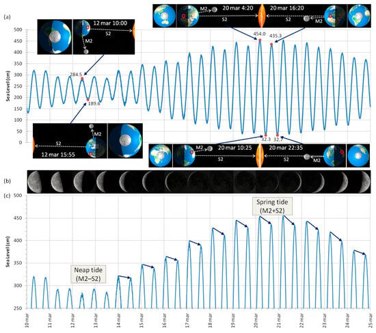
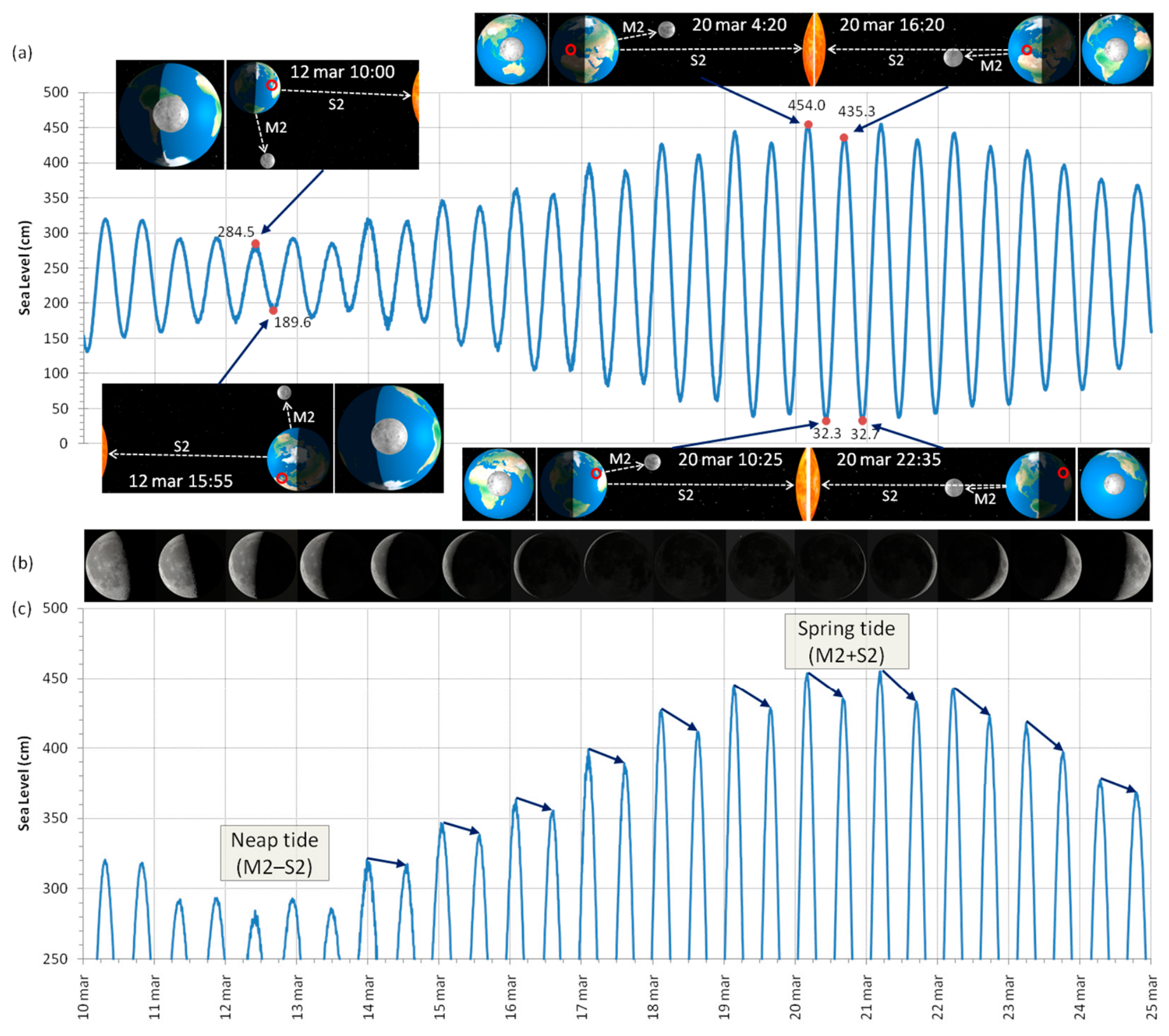
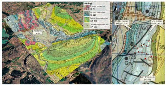
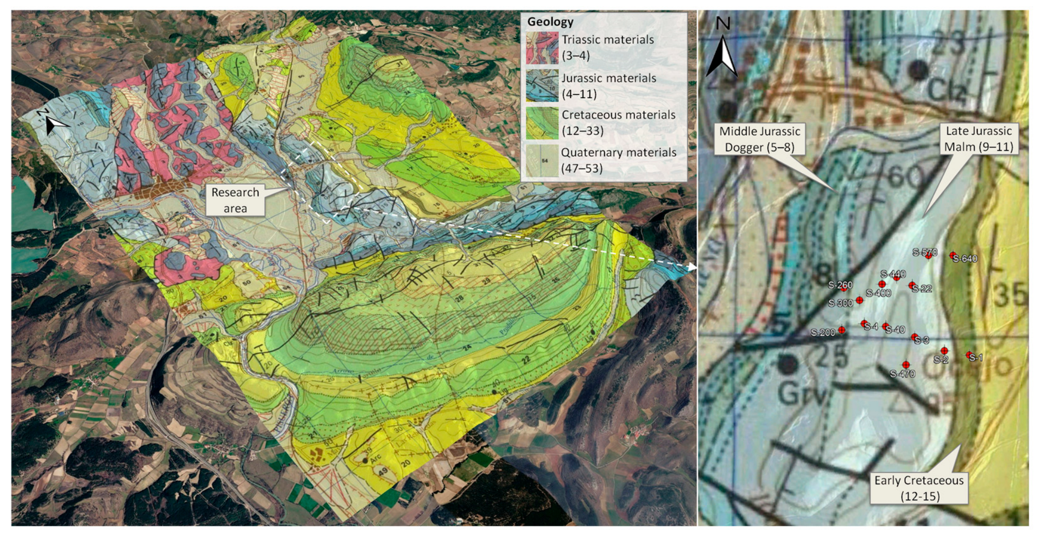
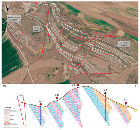
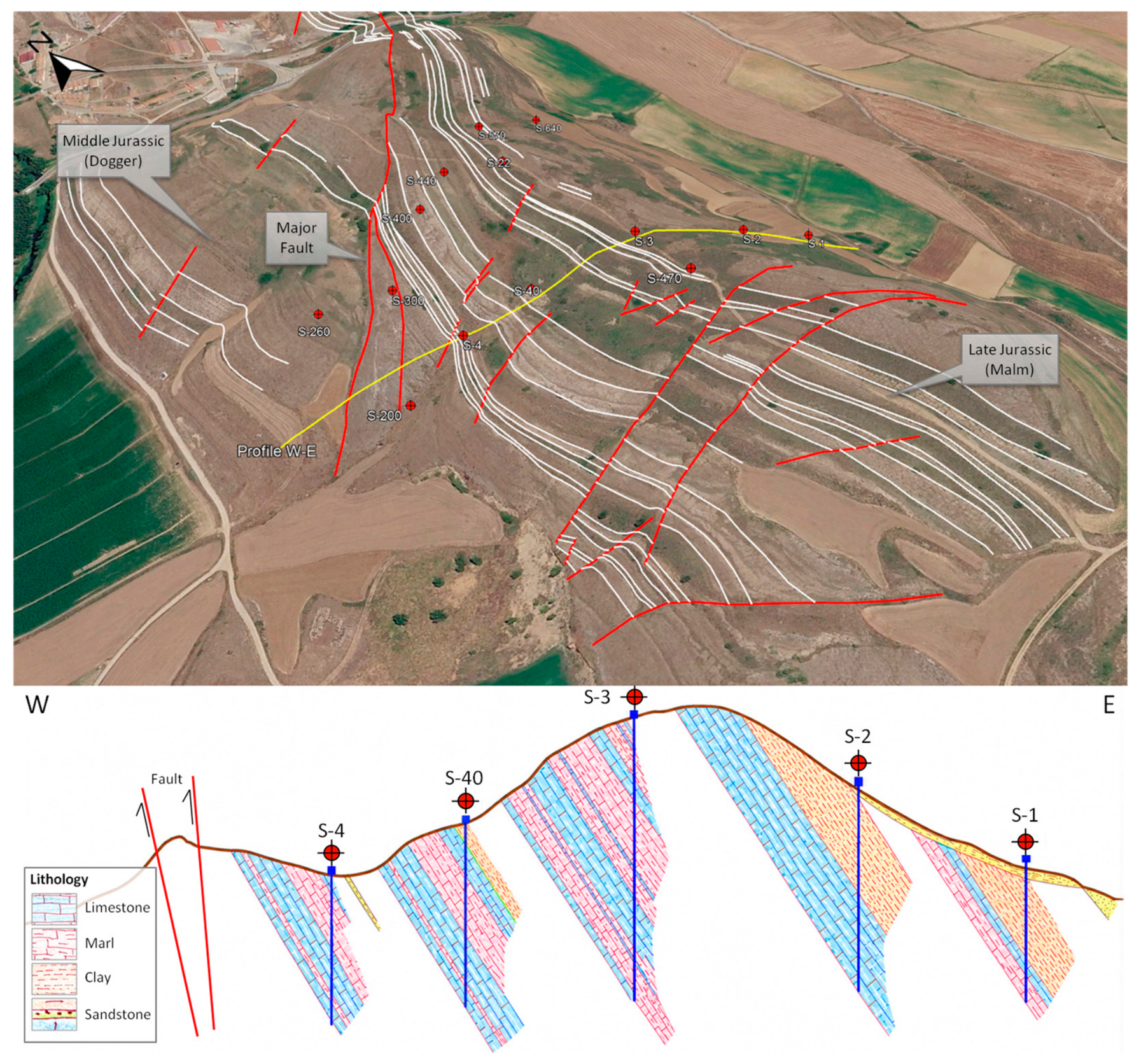
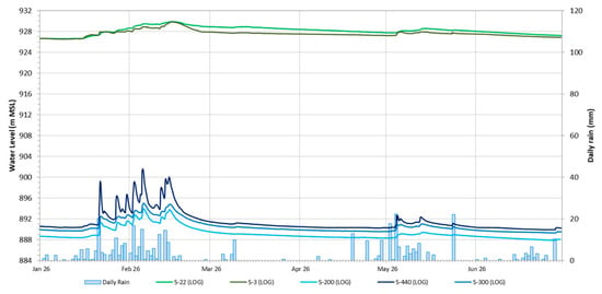
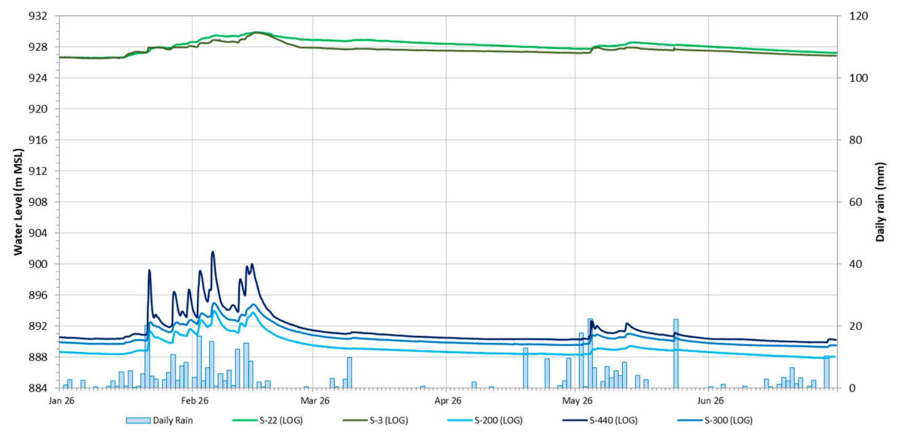
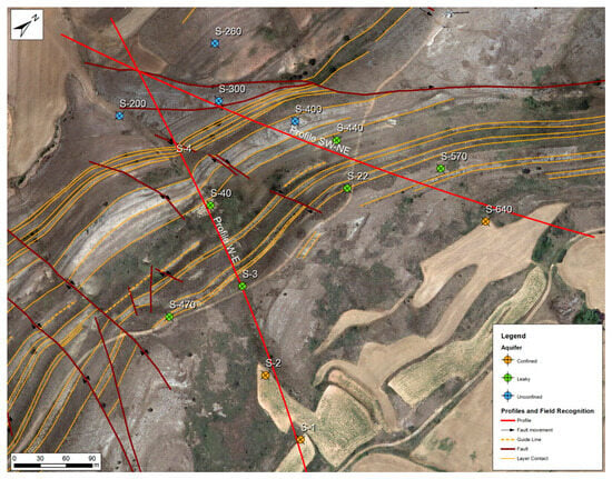
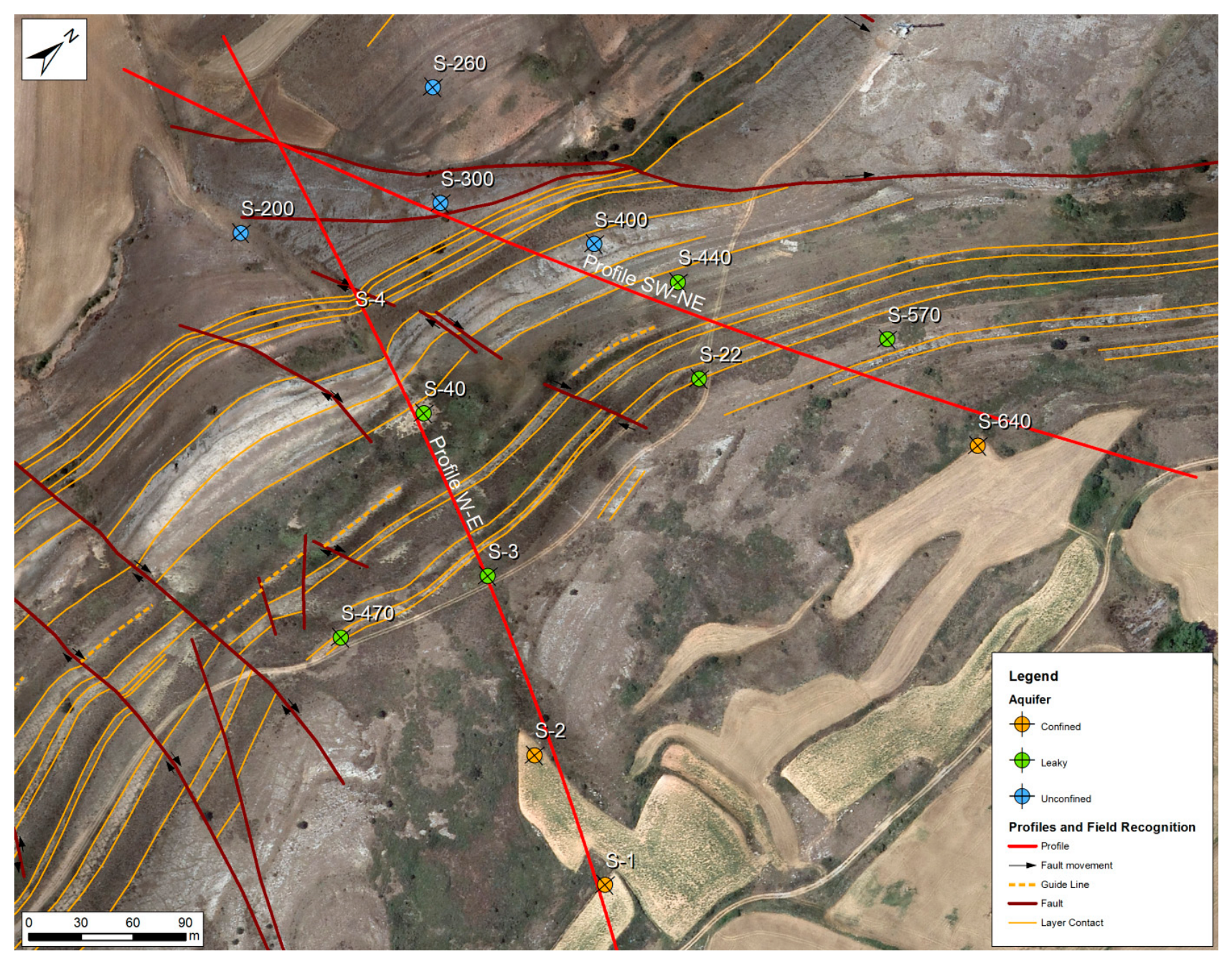
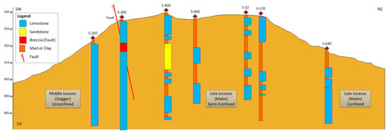
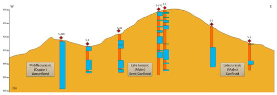
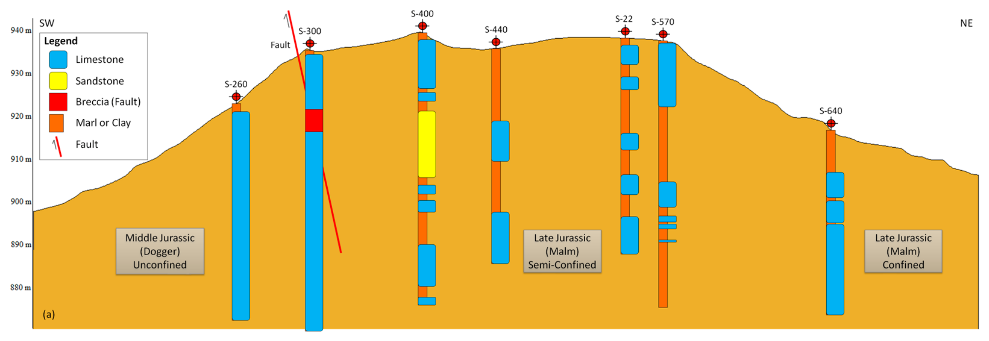
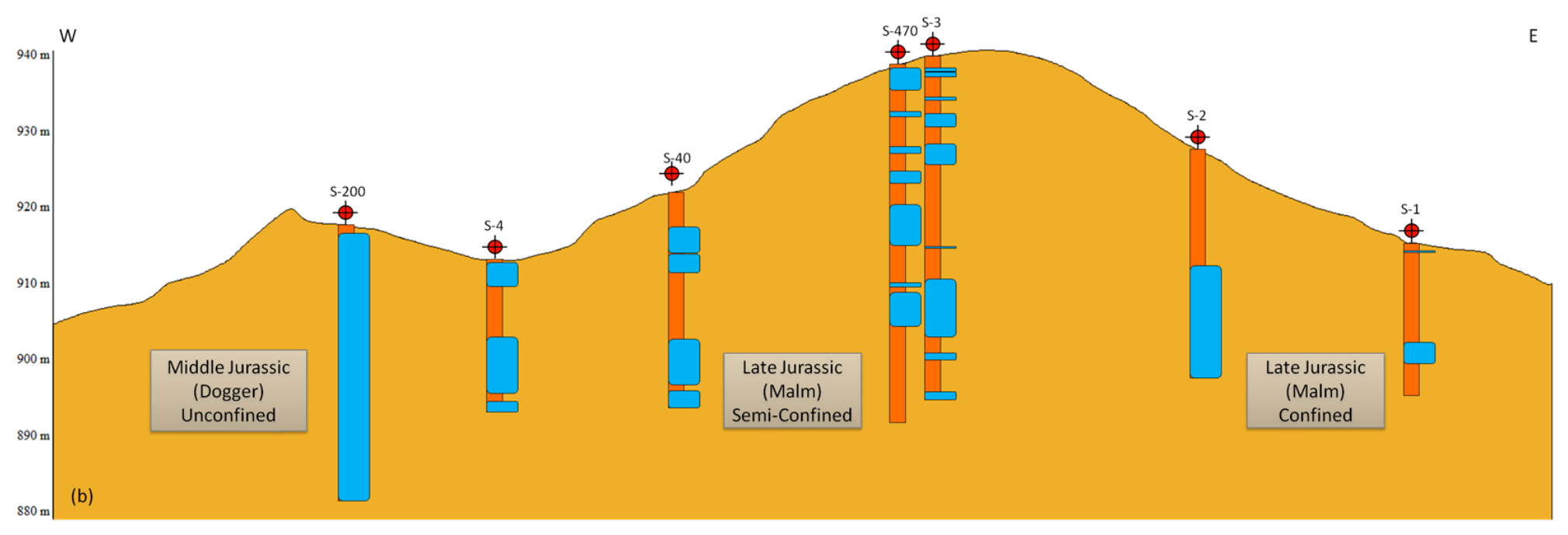
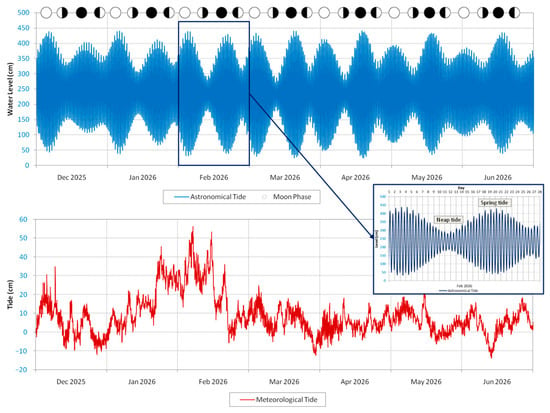
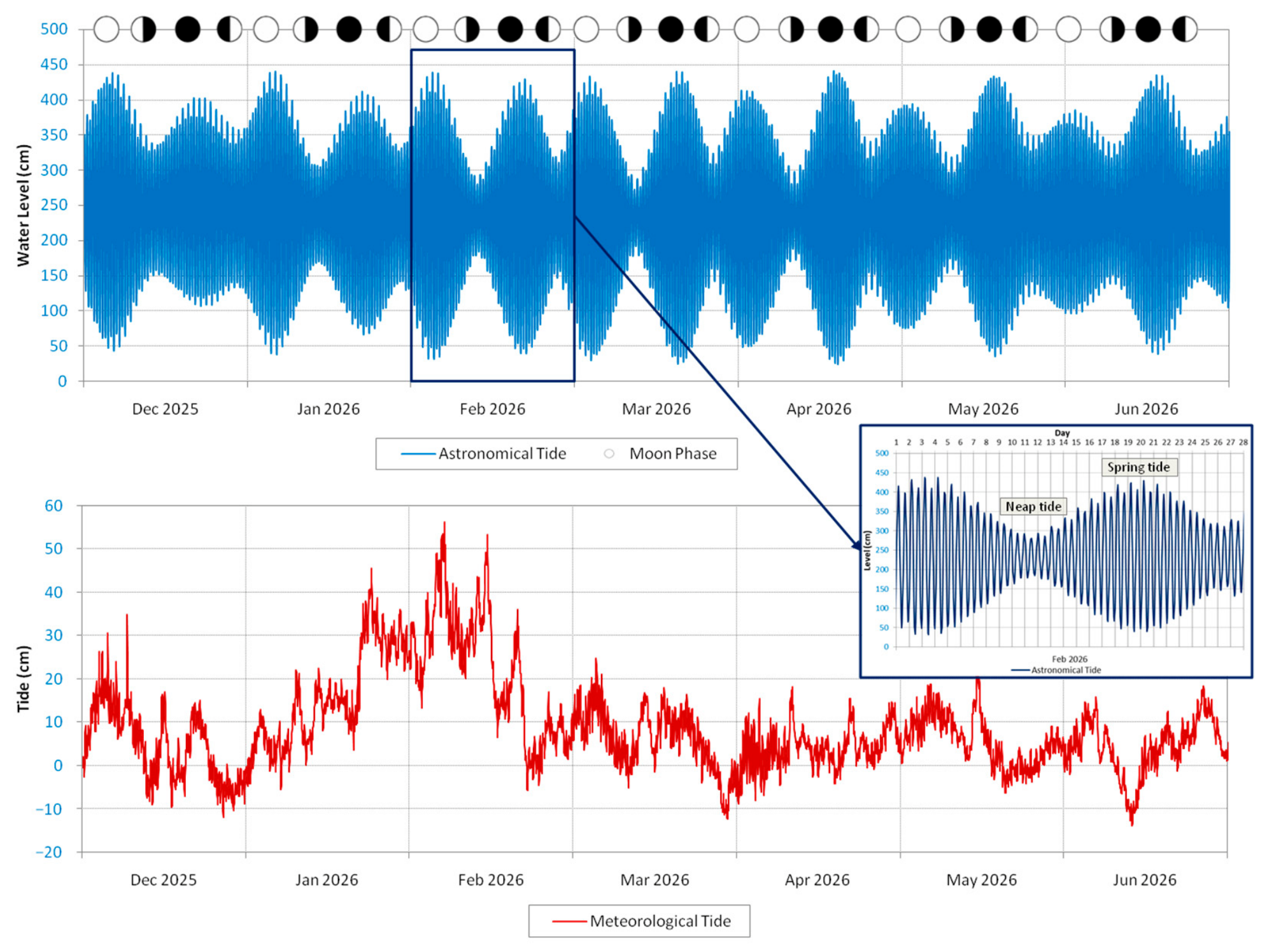
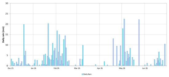
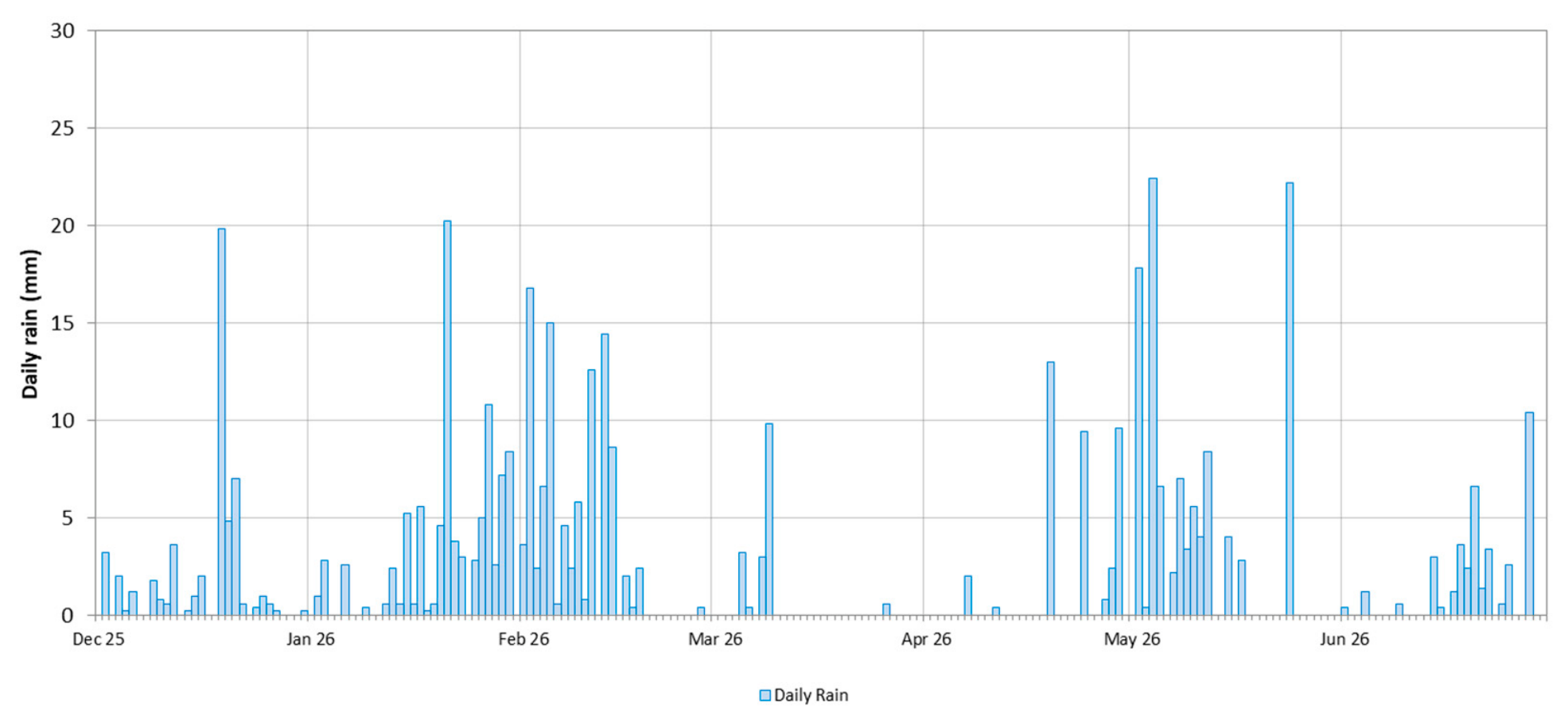
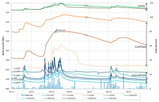
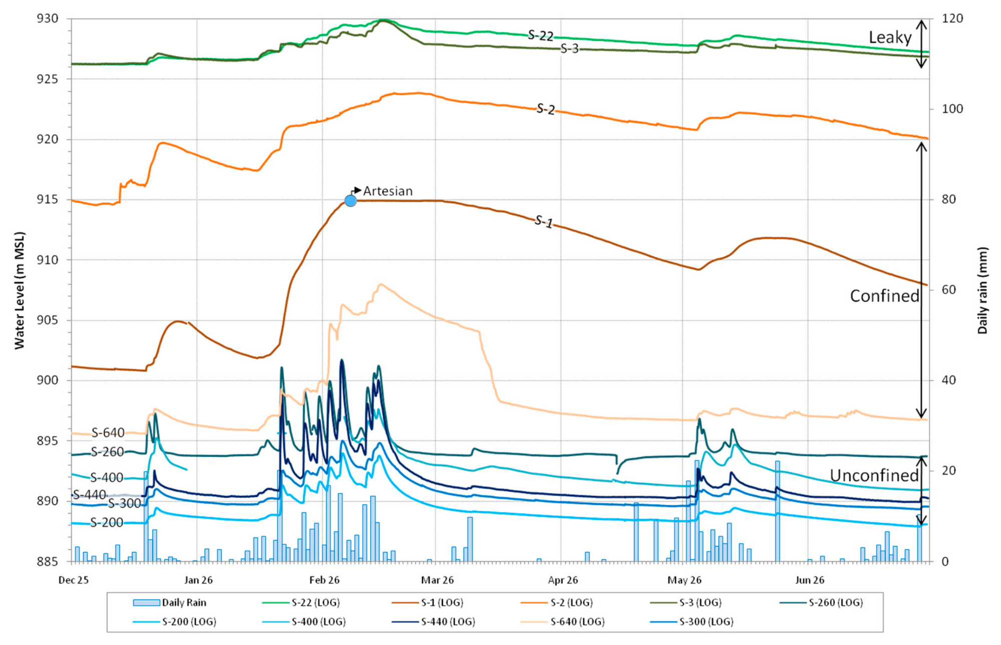
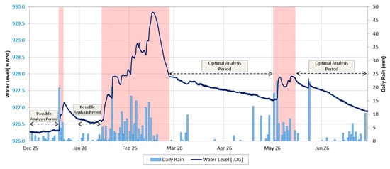
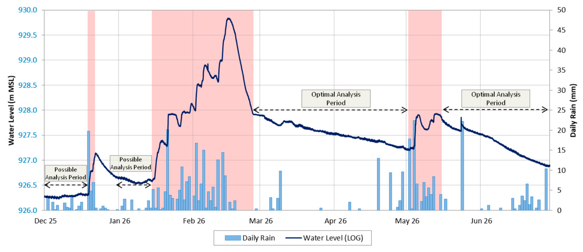
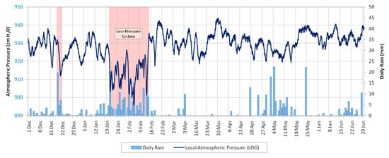
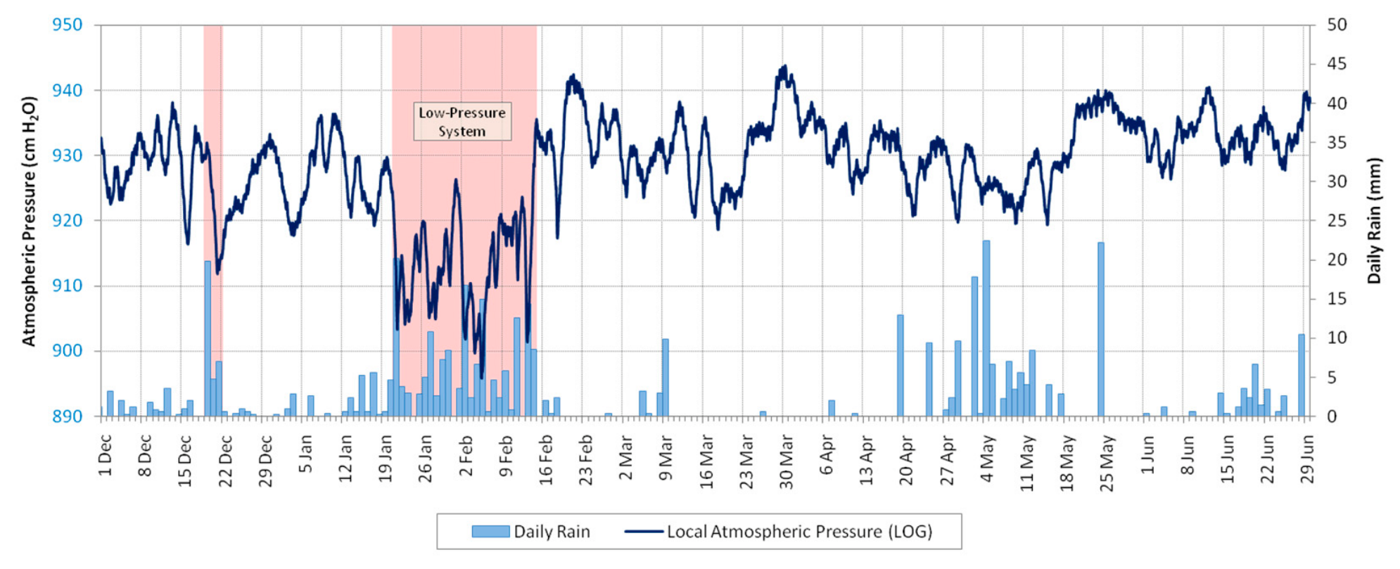
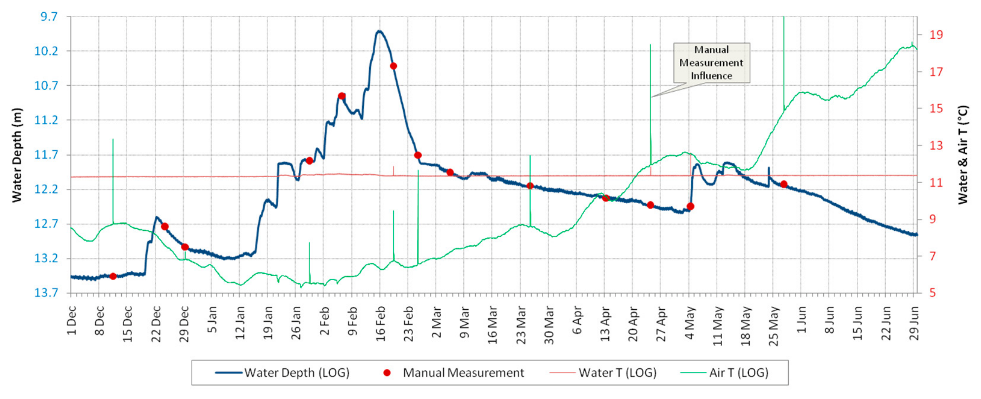
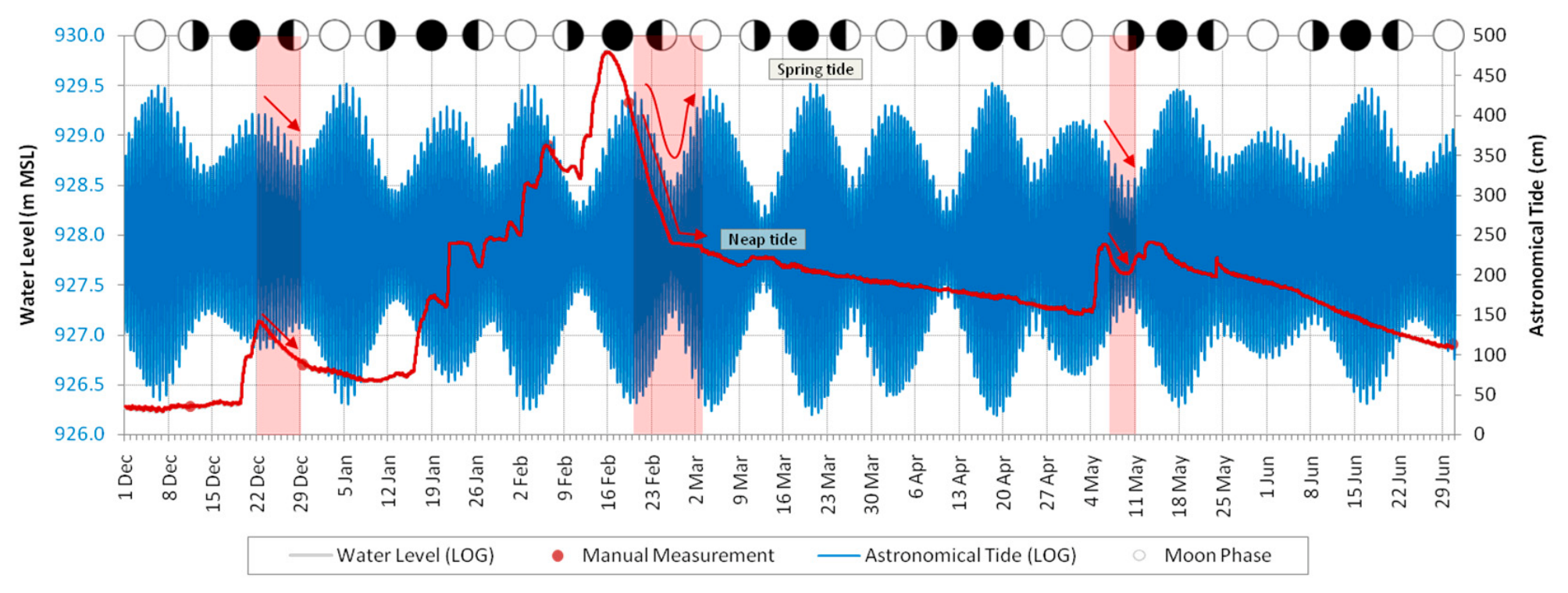
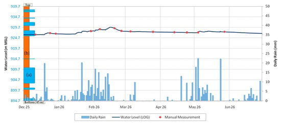
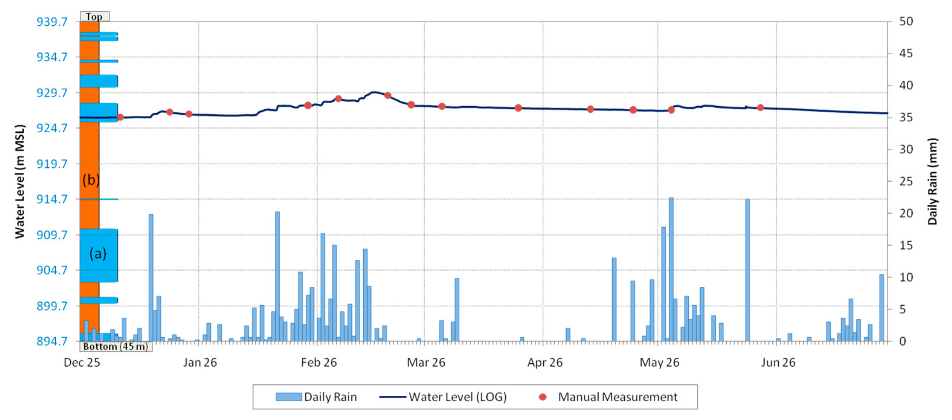
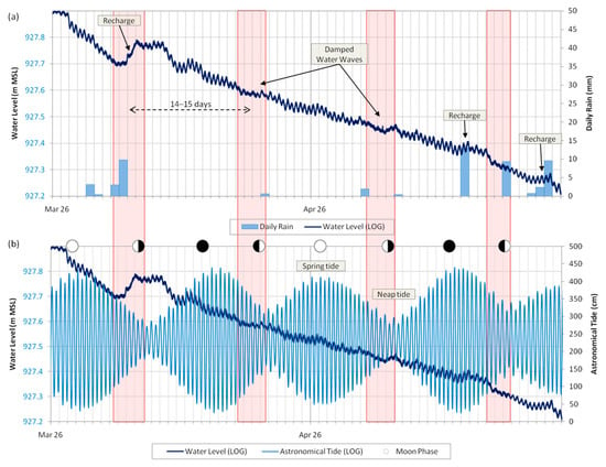
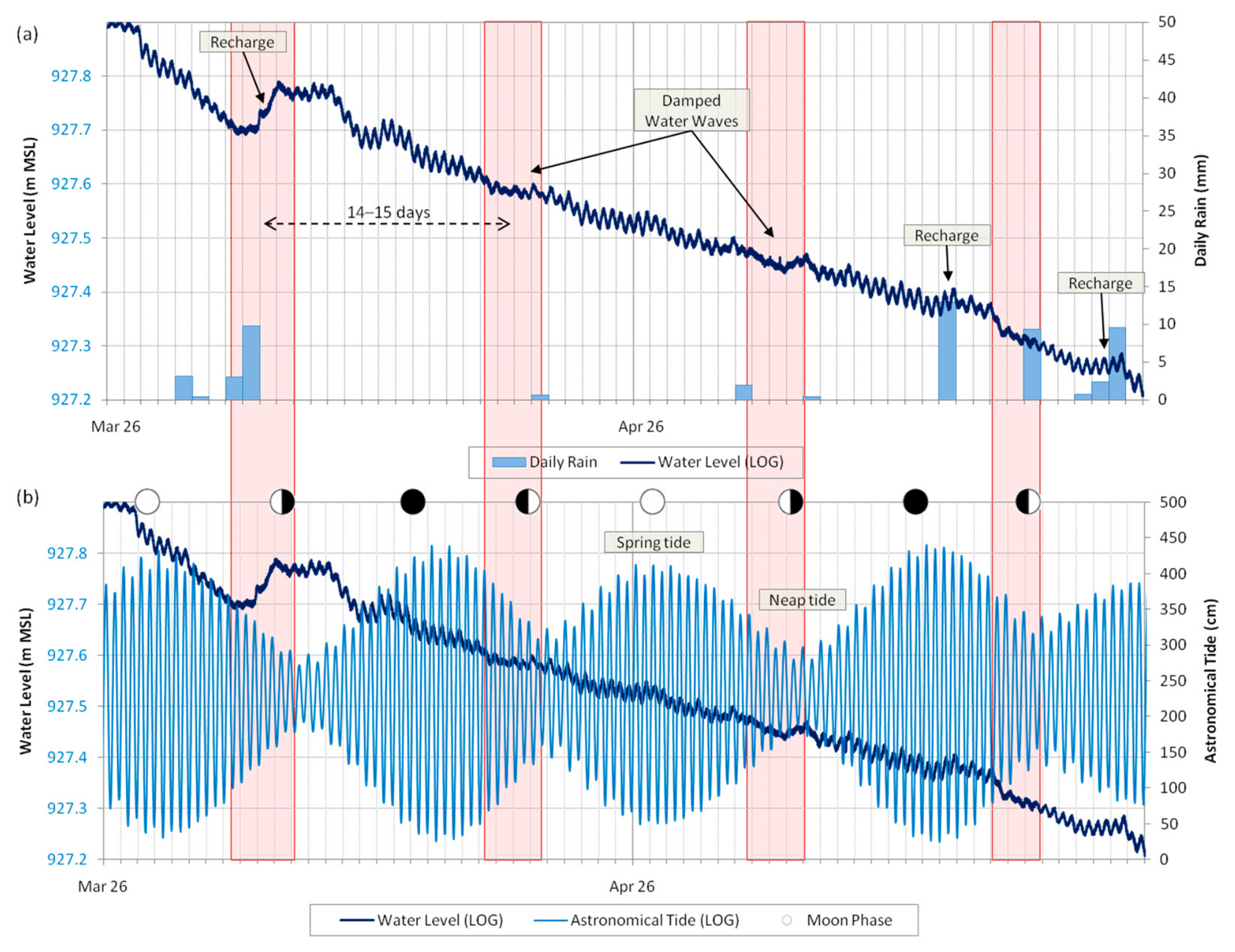
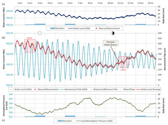
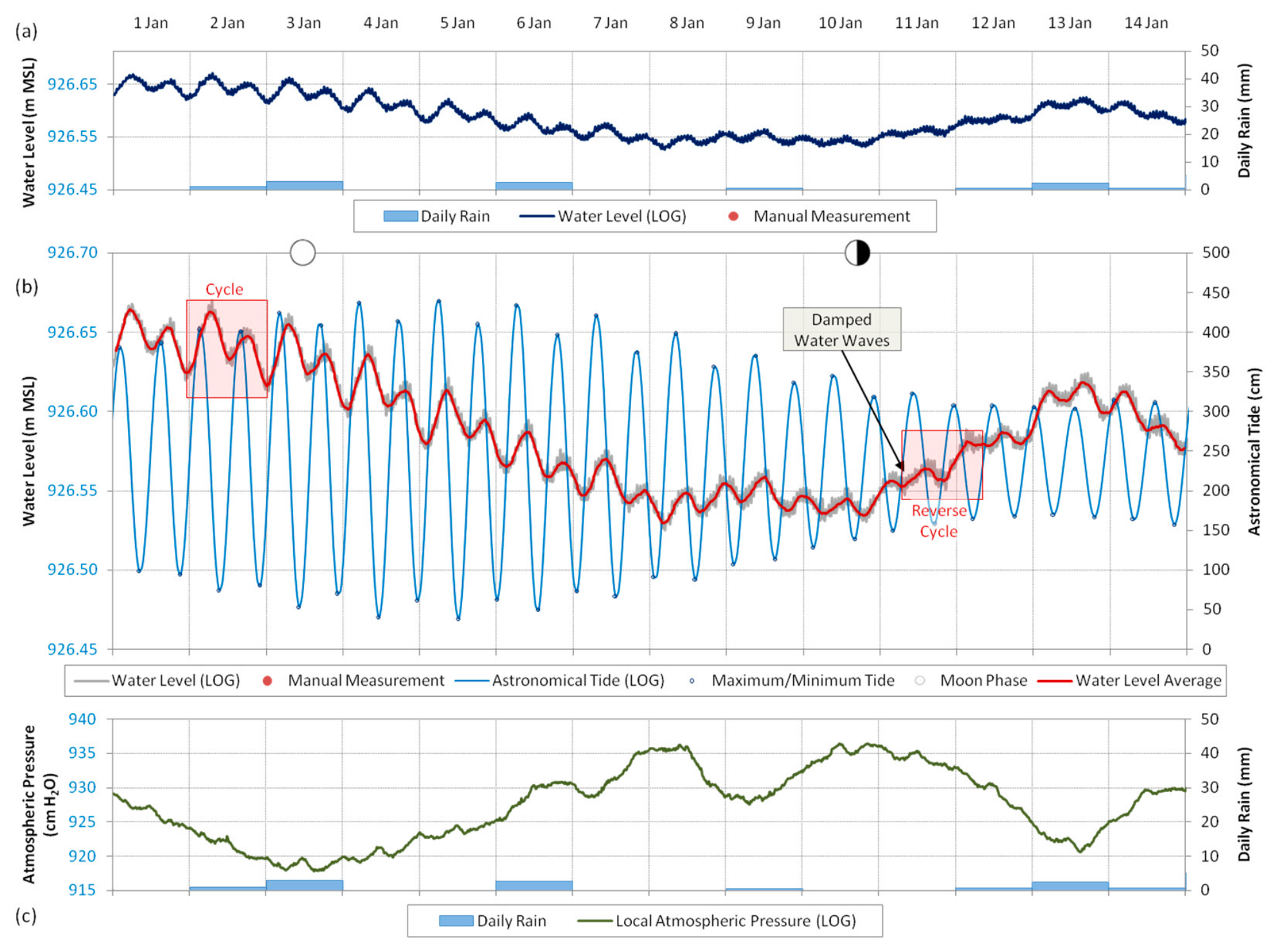
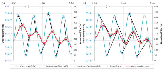
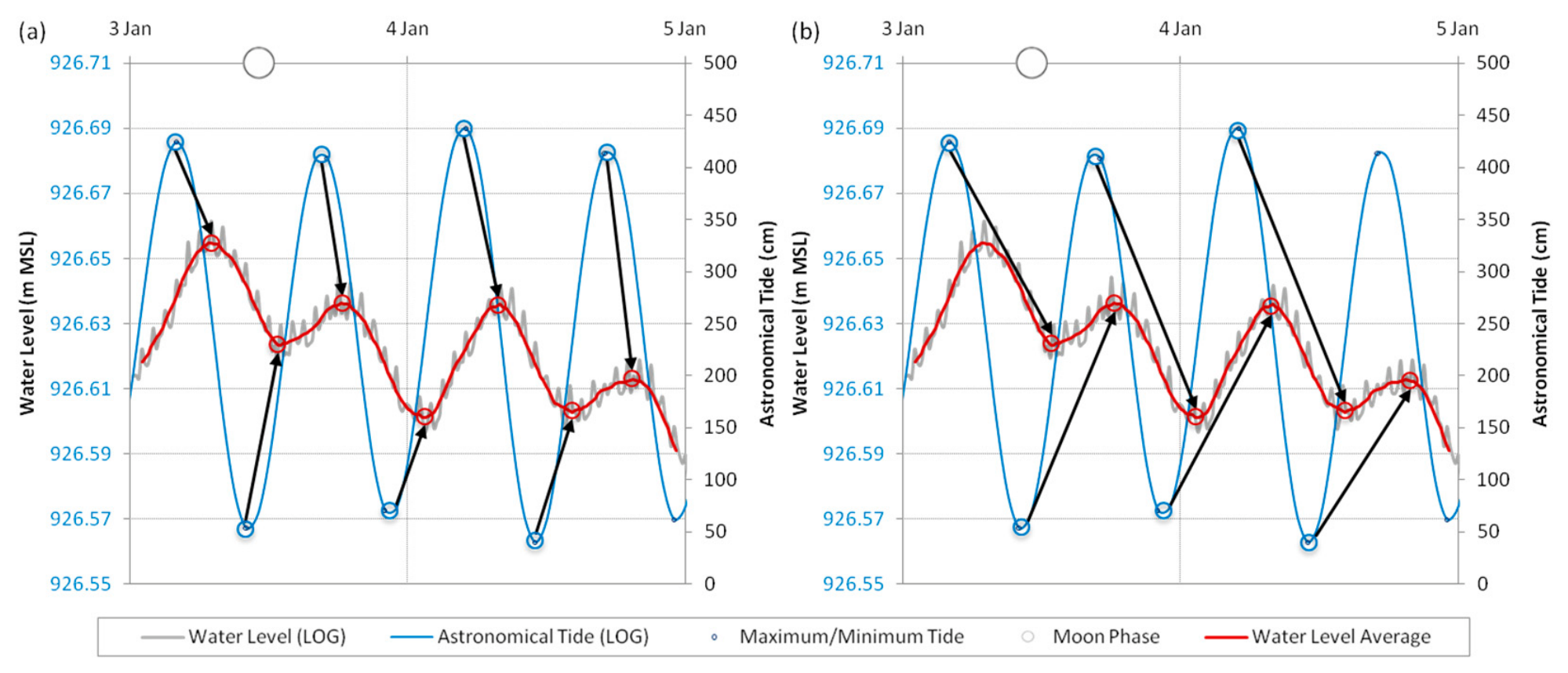
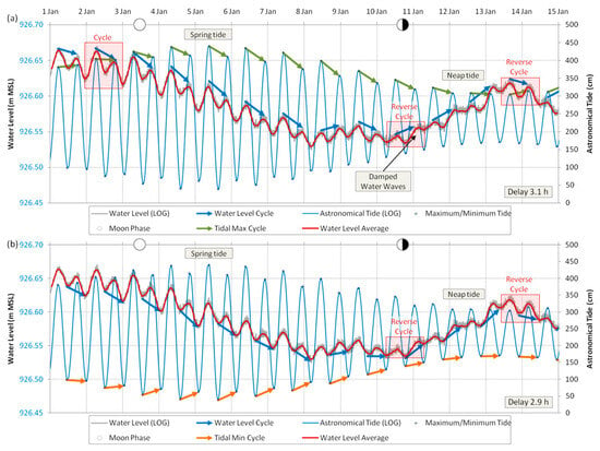
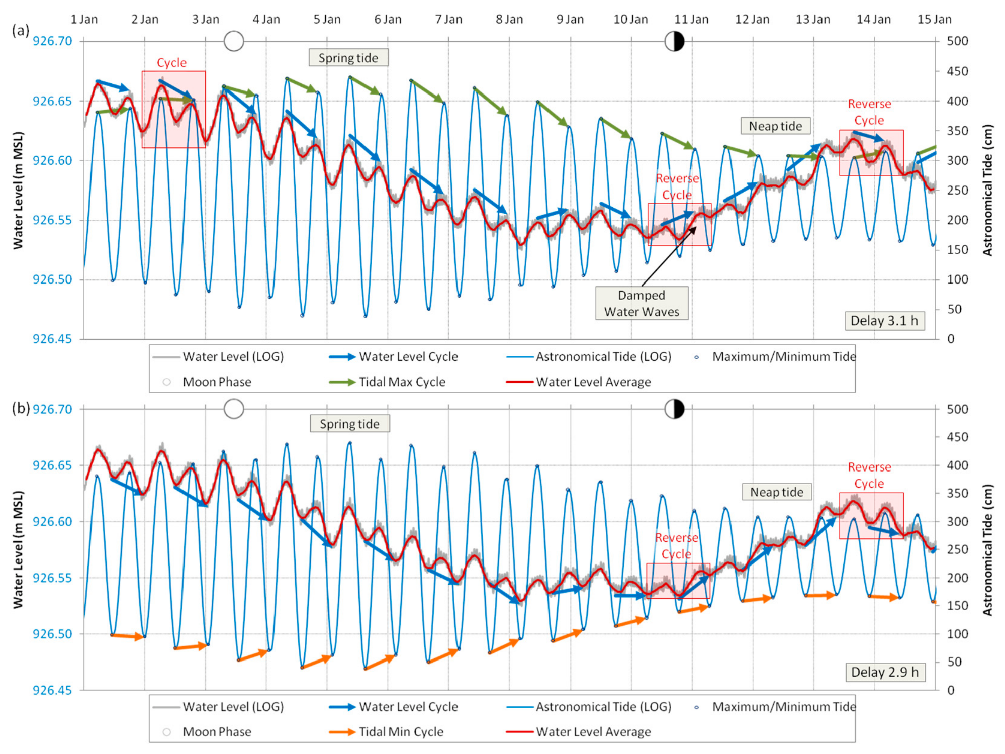
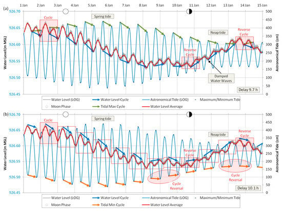
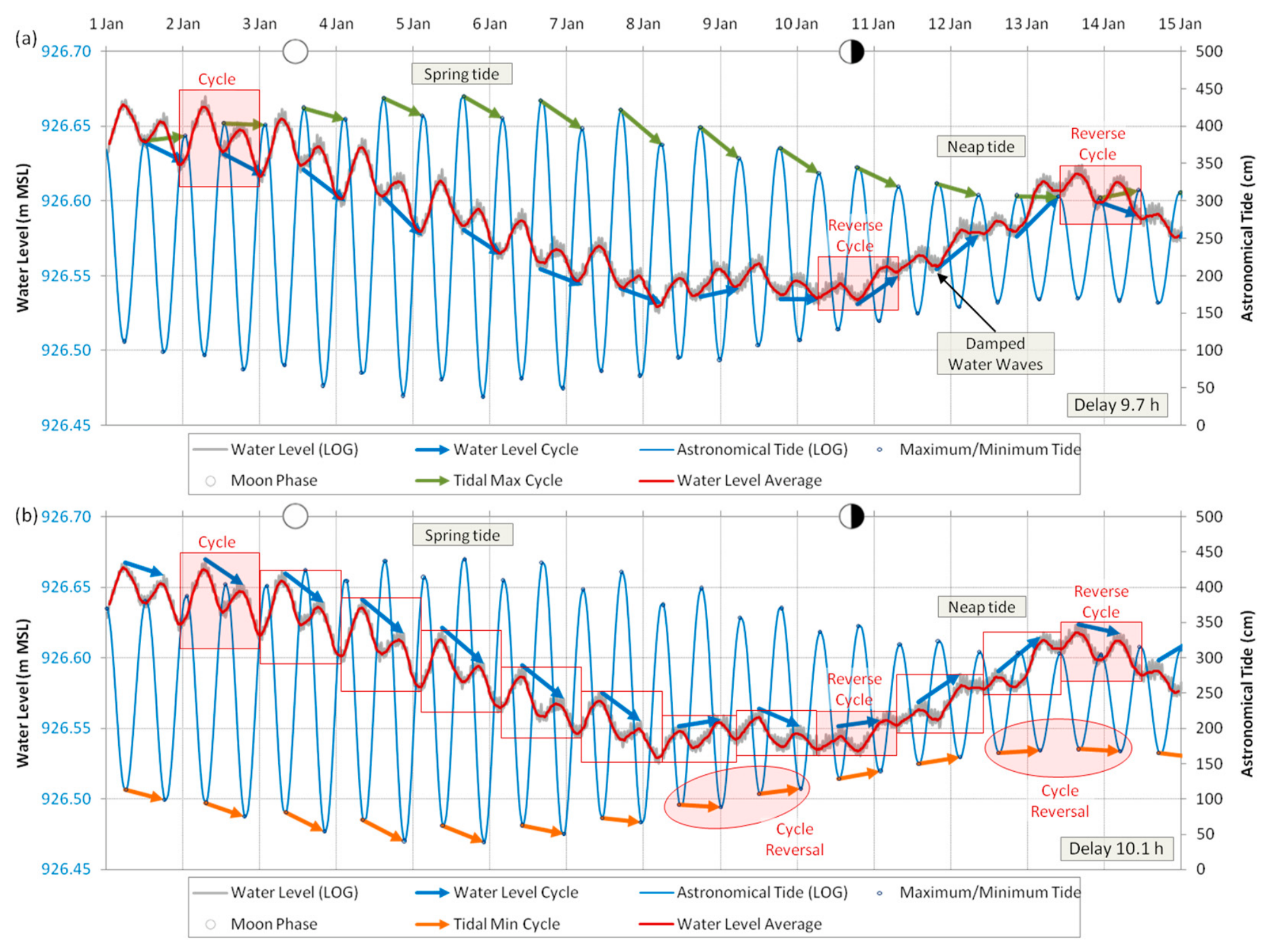
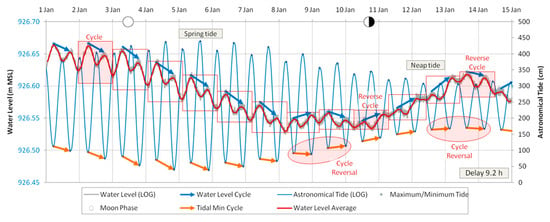
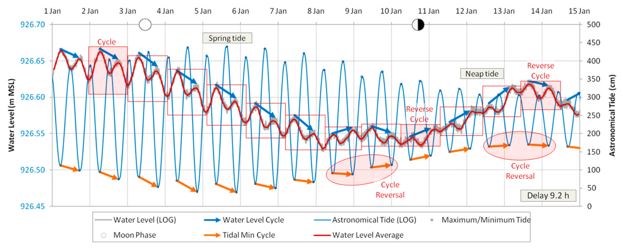
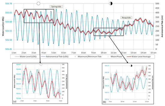
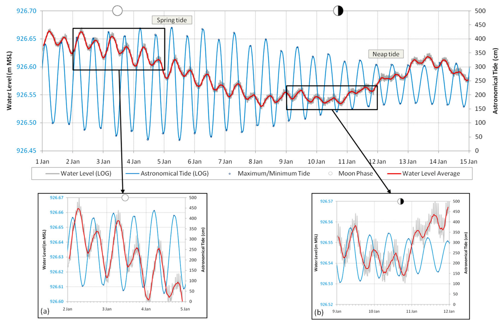
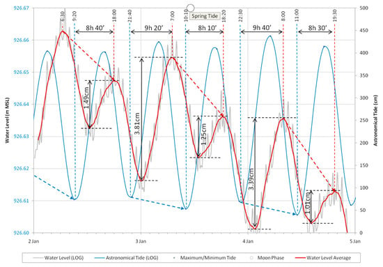
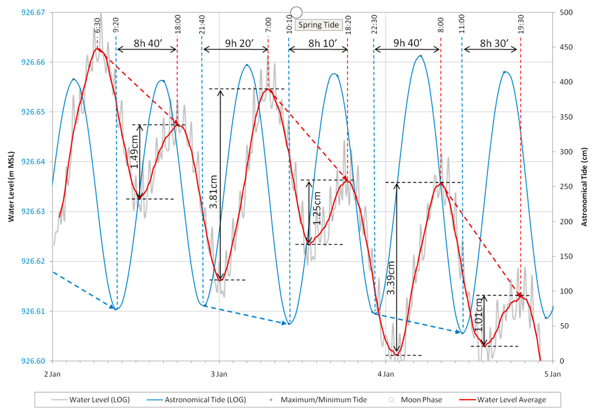
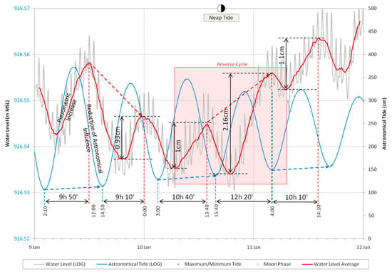
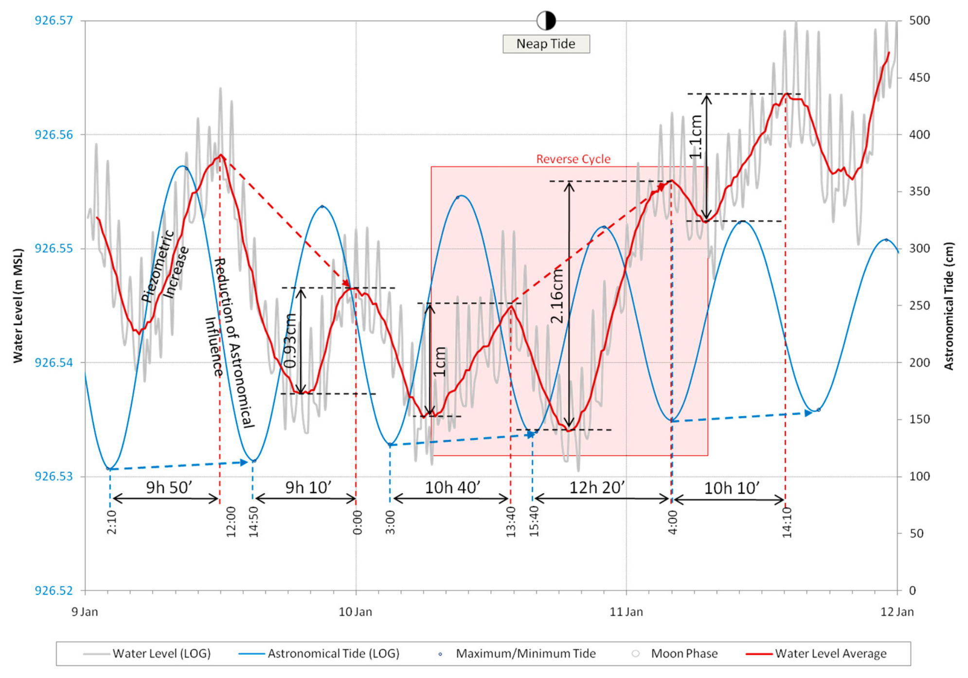
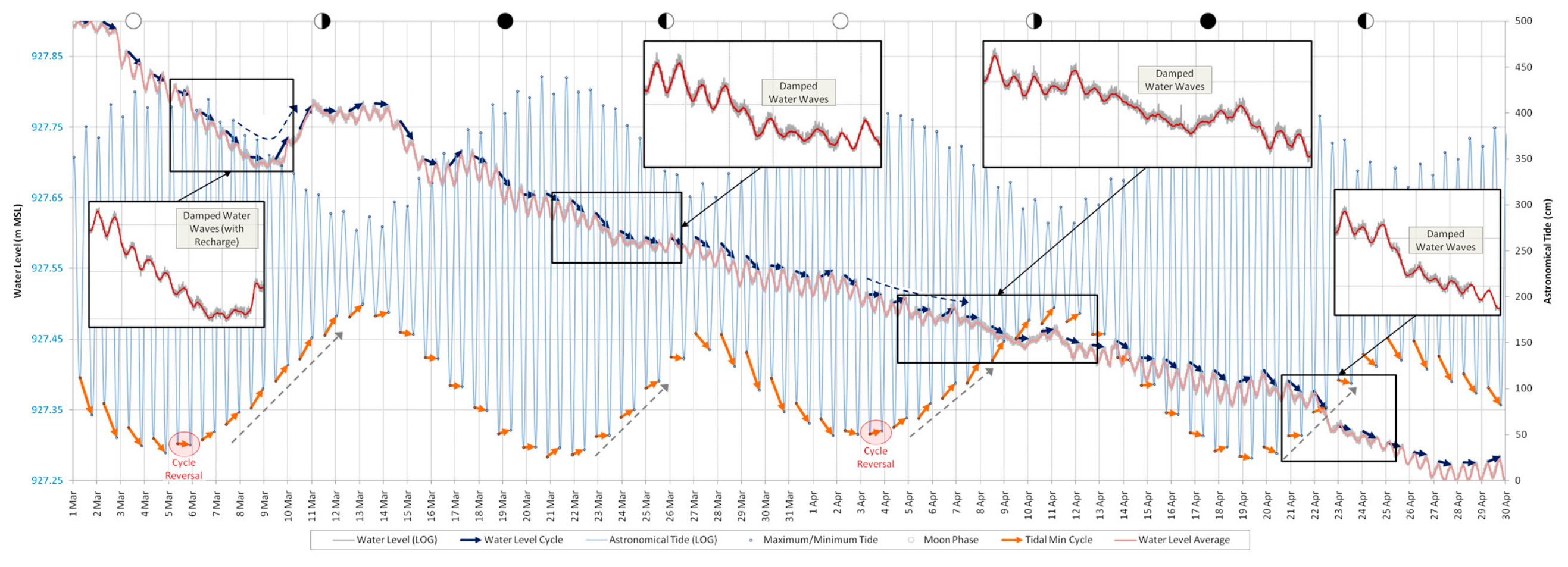
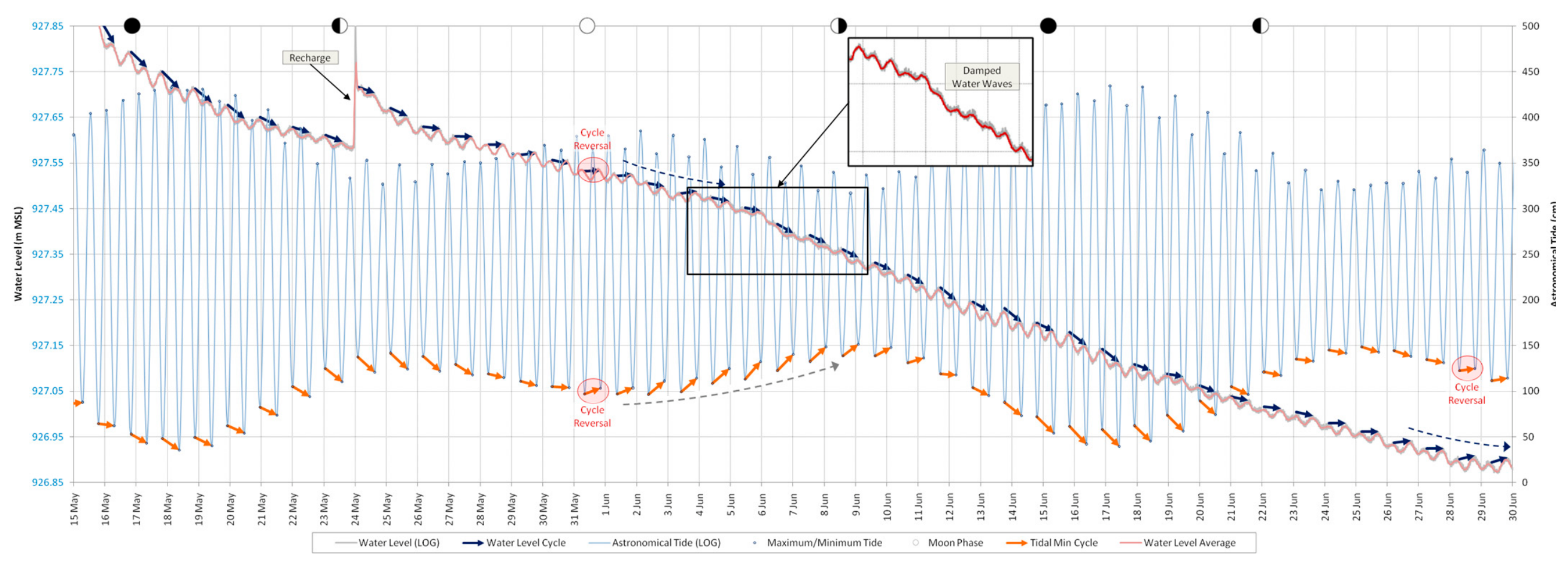
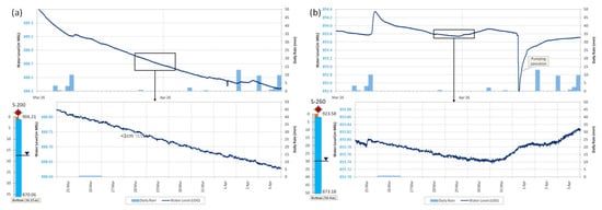
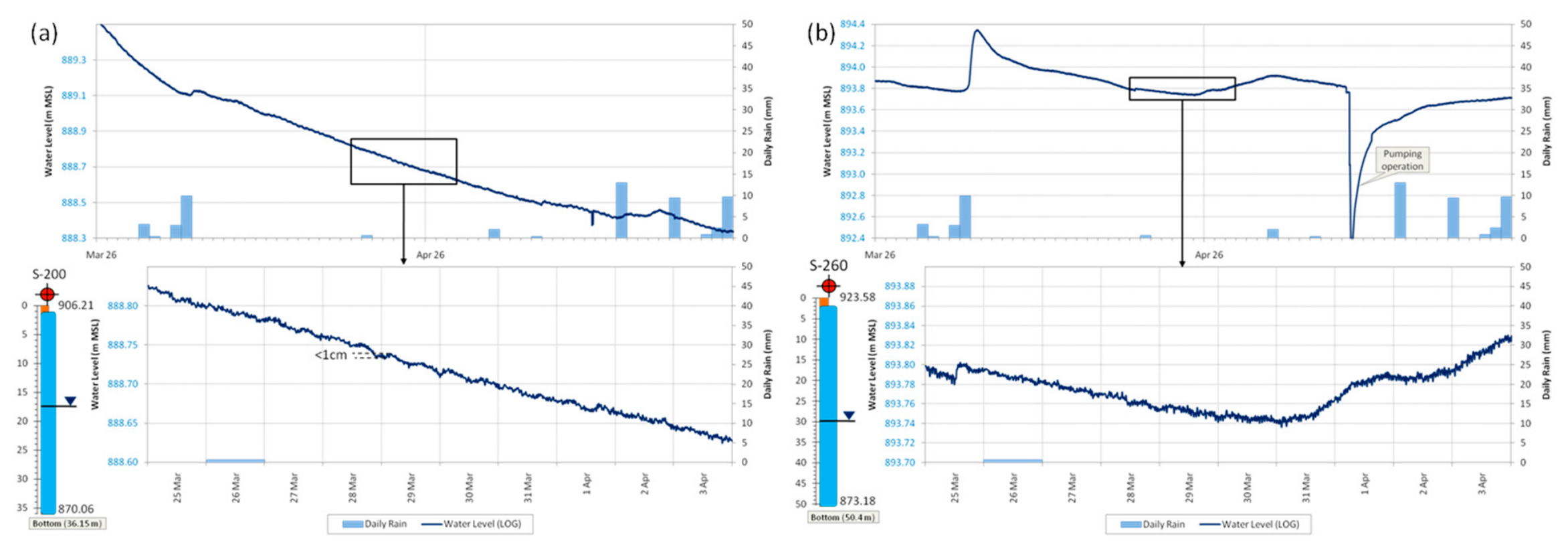
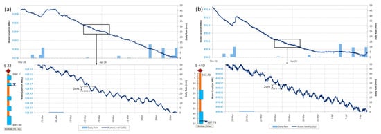
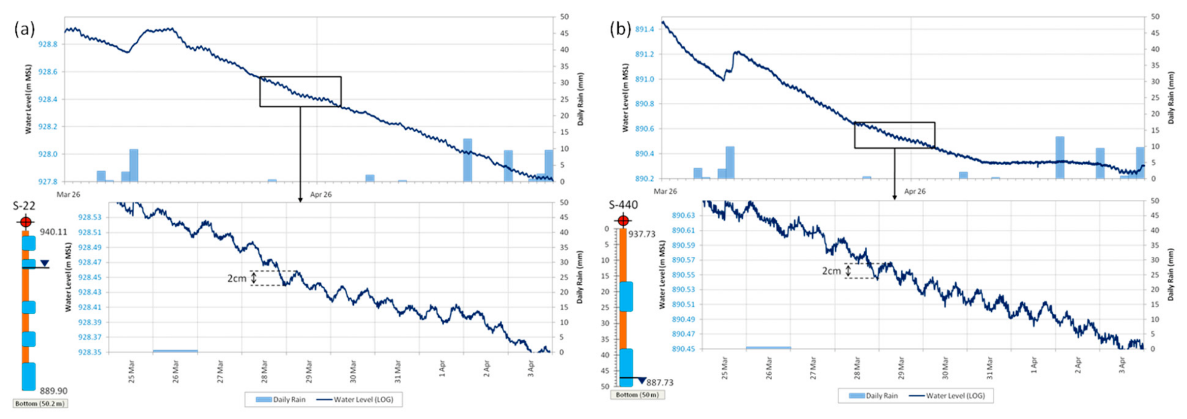
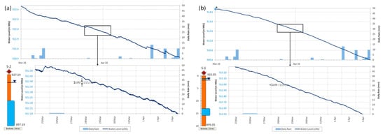
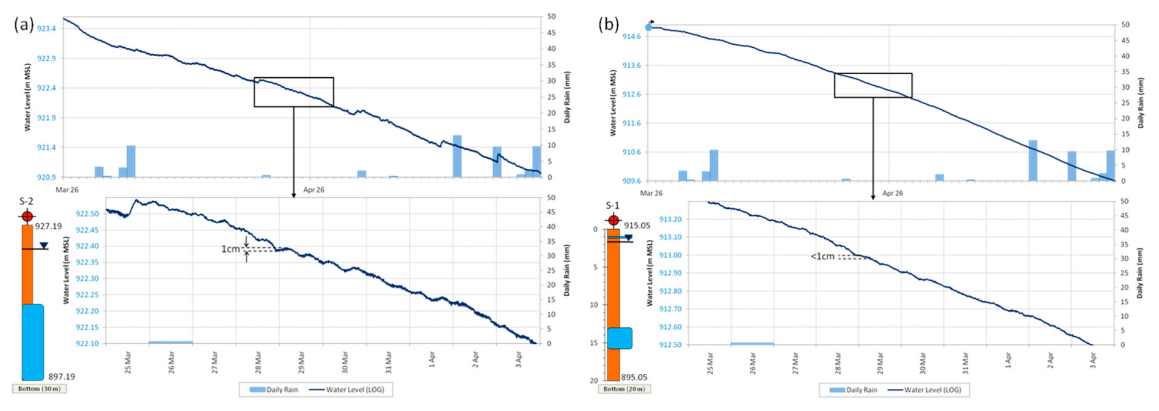
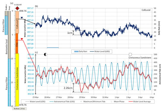
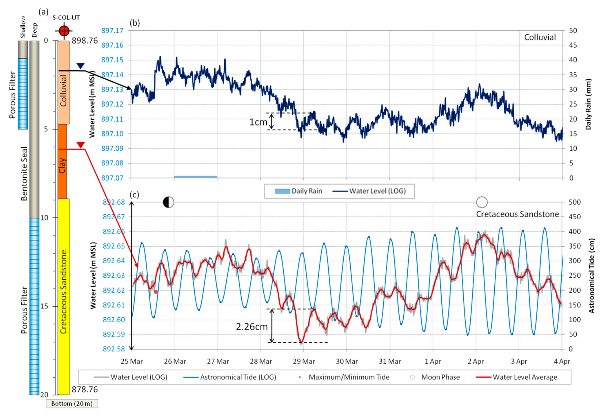
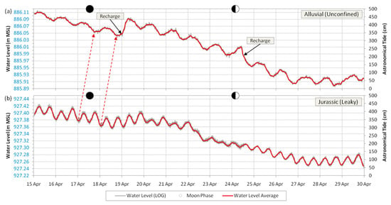
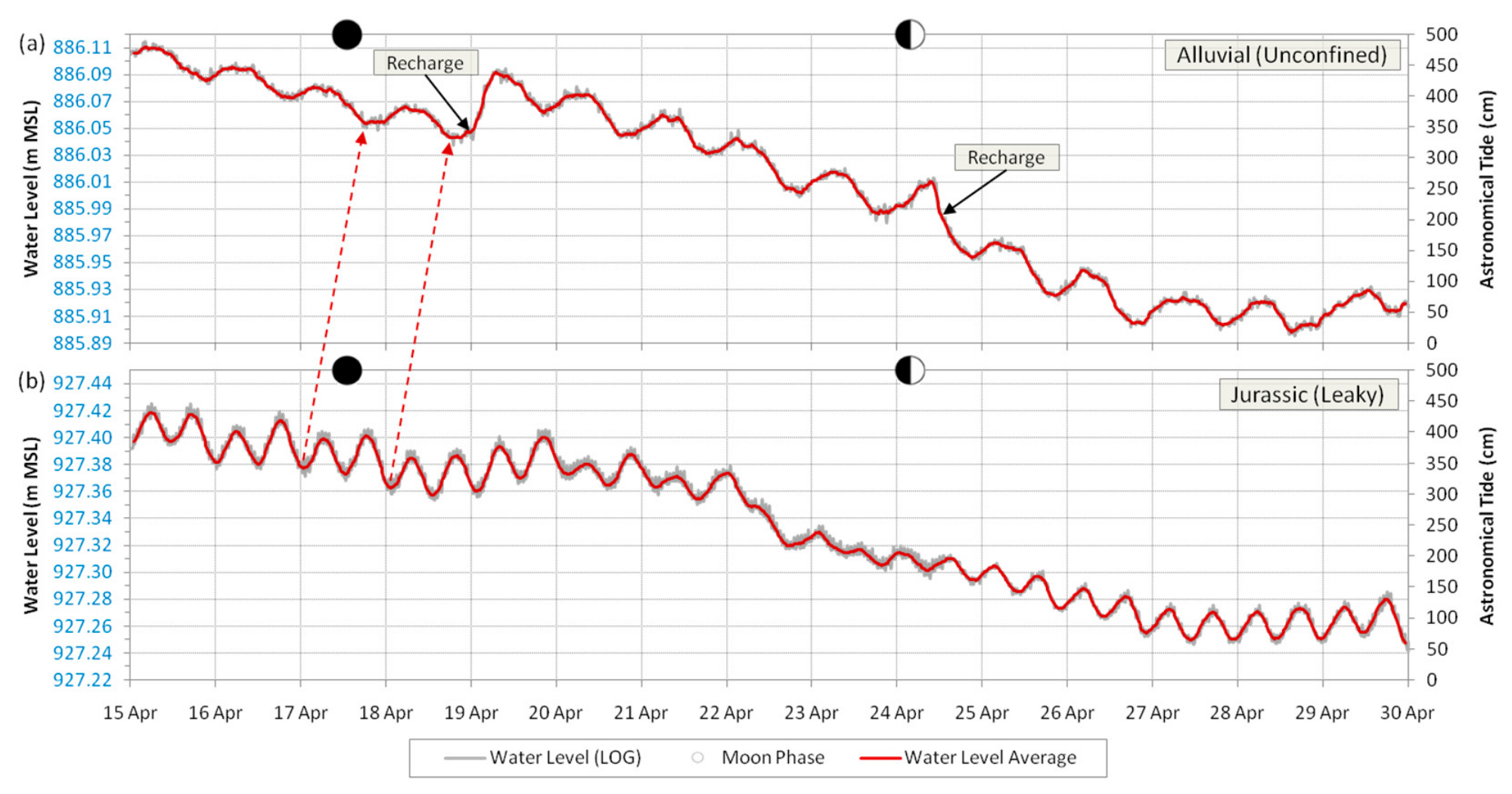
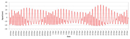
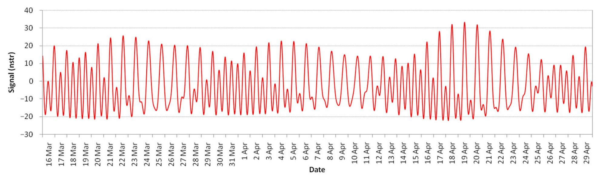
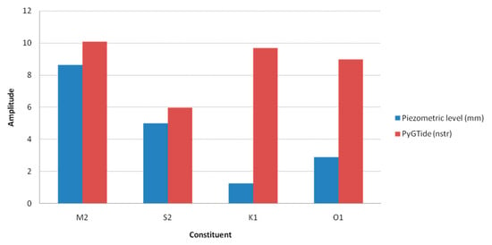
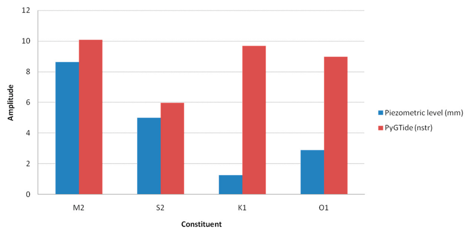
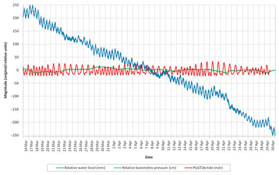
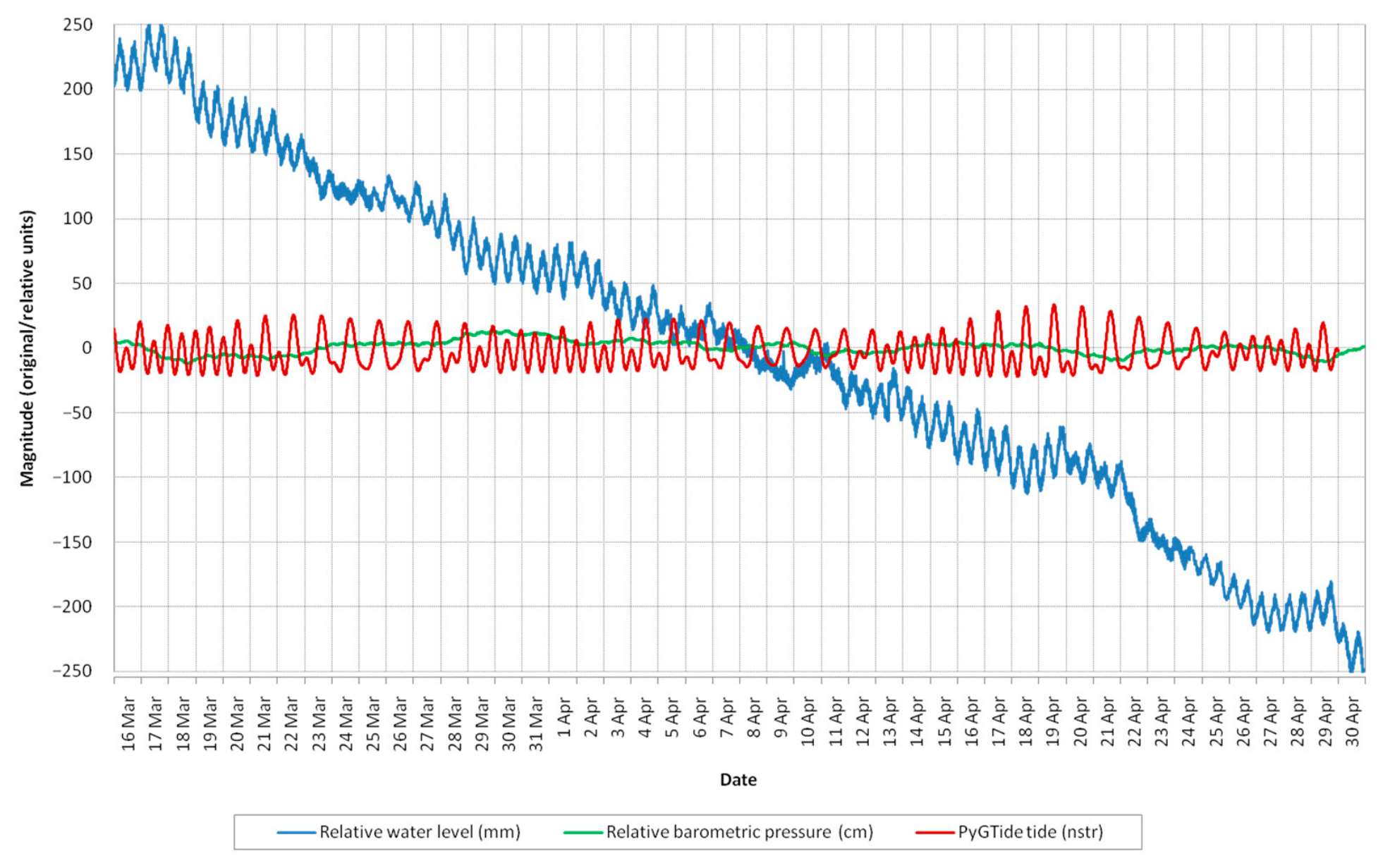

Disclaimer/Publisher’s Note: The statements, opinions and data contained in all publications are solely those of the individual author(s) and contributor(s) and not of MDPI and/or the editor(s). MDPI and/or the editor(s) disclaim responsibility for any injury to people or property resulting from any ideas, methods, instructions or products referred to in the content. |
© 2026 by the authors. Licensee MDPI, Basel, Switzerland. This article is an open access article distributed under the terms and conditions of the Creative Commons Attribution (CC BY) license.