Effects of Vegetation Configuration on Soil Aggregate Stability of Restored Cut Slopes

Abstract

Soil aggregate stability is an important indicator for evaluating the ecological restoration of engineered cut slopes. This study descriptively compared the soil properties and aggregate stability among vegetation treatments in model cut slopes in Wuhan, Hubei Province, Central China. Four treatments were established, each represented by one model slope: bare-slope (BS), grass (GS), shrub (SS), and grass–shrub (GSS). Soils were sampled at 0–10 and 10–20 cm depths approximately two years after vegetation establishment. Soil physicochemical properties and the water-stable aggregate content (WSA), mean weight diameter (MWD), geometric mean diameter (GMD), percentage of aggregate destruction (PAD), and soil erodibility factor (K) were assessed. Vegetated treatments showed a lower bulk density and higher soil organic carbon (SOC) and soil organic matter (SOM) contents than BS. For the 0–20 cm layer, the mean MWD and GMD across the three vegetated treatments were 30.05% and 6.93% higher than those of BS, respectively, whereas the mean PAD and K were 36.31% and 5.90% lower. The GSS had the highest MWD and lowest PAD, whereas the GS had the highest GMD and lowest K. An exploratory Pearson correlation analysis (n = 4) described the associations of SOC and the 1–5 mm macroaggregate fractions with soil aggregate stability indicators; the interpretation was limited to descriptive associations. These findings provide descriptive evidence for evaluating vegetation treatments in cut-slope restoration and may inform the vegetation selection in Central China.

1. Introduction

Soil erosion is the most prevalent land degradation process worldwide [1]. With the extensive development of infrastructure construction, a large number of cut slopes have been formed, whose surfaces are directly exposed to the natural environment for long periods. Due to engineering disturbance and vegetation destruction, the soil degradation and nutrient loss on cut slopes become increasingly severe. The soil structural stability is therefore vulnerable to degradation [2,3]. Consequently, slope erosion and spalling are easily triggered, which may even lead to slope collapse, landslides, and building destruction, seriously challenging engineering safety and the ecological environment [4]. Vegetation restoration is commonly carried out to prevent surface soil and improve the microenvironment after engineering construction [5,6,7]. Soil aggregate is closely related to erosion processes, organic carbon, fertility, and biological community [4,7]. It is an important indicator to reflect the quality of ecological restoration. Therefore, exploring the effects of vegetation restoration on soil aggregate stability and soil erodibility is vitally necessary for evaluating ecological construction performance and optimizing ecological management.

Soil aggregates are basic units of soil structure, generally with diameters of <10 mm, and are closely related to soil physicochemical properties and structural stability. Previous studies have pointed out that soil aggregate stability is influenced by multiple factors [8,9,10,11]. For instance, the soil bulk density is closely related to the soil pore structure and water movement, which may further influence aggregate stability and erosion resistance [9]. The aggregation degree and stability of the soil at various particle sizes are important physical properties that determine soil erodibility [10]. Soil organic carbon (SOC) can bind small soil particles into larger ones and promote the aggregation process [12]. The vegetation configuration also affects soil aggregate stability. With continued plant growth, the content of large aggregates may increase. The soil aggregate structure tends to stabilize as the vegetation community succession progresses [13]. As for cut slopes formed during engineering construction, the surface soil structure and fertility gradually degrade due to artificial disturbance and the absence of vegetation cover. Soil aggregates are disintegrated and fragmented into smaller, more easily transported soil particles and microaggregates by external forces such as rainfall erosion. Such processes disrupt the soil aggregate structure and provide erodible materials for soil particle detachment and subsequent sediment transport [14,15]. Furthermore, soil water retention and the plant growth environment may also be considerably altered [16]. Therefore, evaluating the effects of different vegetation configurations on soil aggregate stability and erodibility is important for improving ecological restoration strategies for cut slopes.

As aforementioned, vegetation can affect soil–water interactions, leading to changes in the microtopographic characteristics and physicochemical properties of surface soil through hydromechanical effects, including soil stabilization, rainfall interception, runoff and sediment reduction, and root water uptake [5,7]. Vegetation restoration is therefore an important means to reduce soil erosion and achieve ecological reconstruction. Some studies have reported the impacts of vegetation on soil physicochemical properties and the anti-erosion capacity. Ali et al. [17] pointed out that the crop roots affect aggregate stability through soil internal forces, van der Waals attractive force, and surface hydration repulsive forces. Li et al. [18] found that the fungal inoculation increased polysaccharide production and aggregate stability in the compacted soil vegetated with Cynodon dactylon. Zhao et al. [19] claimed that the treatments of vegetation restoration significantly modified the runoff hydrodynamic parameters through the hydromechanical effects of plants. Previous studies suggest that soil physicochemical properties, aggregate stability, and erodibility may vary among plant species. Such differences may further affect the distribution, stability, and nutrient content of soil aggregates. In addition, the inputs of organic matter, water, and temperature in surface soil also differ from each other due to different litters, which, in turn, affect the soil aggregation process. Therefore, a reasonable vegetation configuration pattern is crucial to carrying out cut slope prevention and ecosystem reconstruction. The differences in soil physicochemical properties and aggregate stability among different vegetation configurations therefore need to be clarified. The relationships between soil physicochemical properties and aggregate stability under different vegetation configurations also need to be further explored. However, current works of research mainly focus on the fields of agriculture [17], ecology [20], and forestry [21]. Studies in other regions have also reported that the vegetation type and root characteristics are closely related to soil aggregate stability and erosion resistance [13,22], while different vegetation covers may lead to different soil–water responses on slopes [23]. Previous studies have investigated the relationships between the vegetation configuration and SOC in different regions and ecosystems, including the Loess Plateau [24], artificial forests [23], desert [25], and karst regions [26]. Cut slope is a characteristic type of land degradation that is typically represented by severe soil loss and vegetation destruction. High-intensity human disturbance can lead to the fragmentation of large macroaggregates and an increased proportion of microaggregates [27,28]. Under heavy rainfall, soil aggregates on disturbed cut slopes can be fragmented, resulting in decreased soil structural stability and increased soil erodibility. However, current studies on the ecological restoration of cut slopes have mainly focused on root reinforcement and runoff erosion reduction, while comparative studies on the effects of different vegetation configurations on soil aggregate composition and stability remain limited. Therefore, it is imperative to compare the effects of different vegetation configurations on soil aggregates and identify a suitable pattern for bare cut slopes.

To address the aforementioned research gap, this study aimed to explore the effects of different vegetation treatments on the soil aggregate stability of cut slopes. To achieve this objective, Cynodon dactylon and Magnolia multiflora were selected because they are widely distributed in Central China and commonly used for slope restoration, and three vegetation treatments were accordingly designed, namely, grass, shrub, and grass–shrub. Then, model experiments under different vegetation treatments were conducted. Soil physicochemical properties were compared among the three vegetation treatments and the bare-slope control. The differences in soil aggregate stability indicators among vegetation treatments were analyzed. The relationship between soil aggregate stability and soil erodibility was examined. Finally, factors associated with soil aggregate stability and erodibility were identified using correlation analysis. The findings can provide a reference for selecting appropriate vegetation restoration strategies for cut slopes in Central China.

2. Materials and Methods

2.1. Model Slope Construction

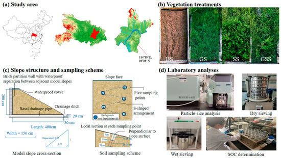
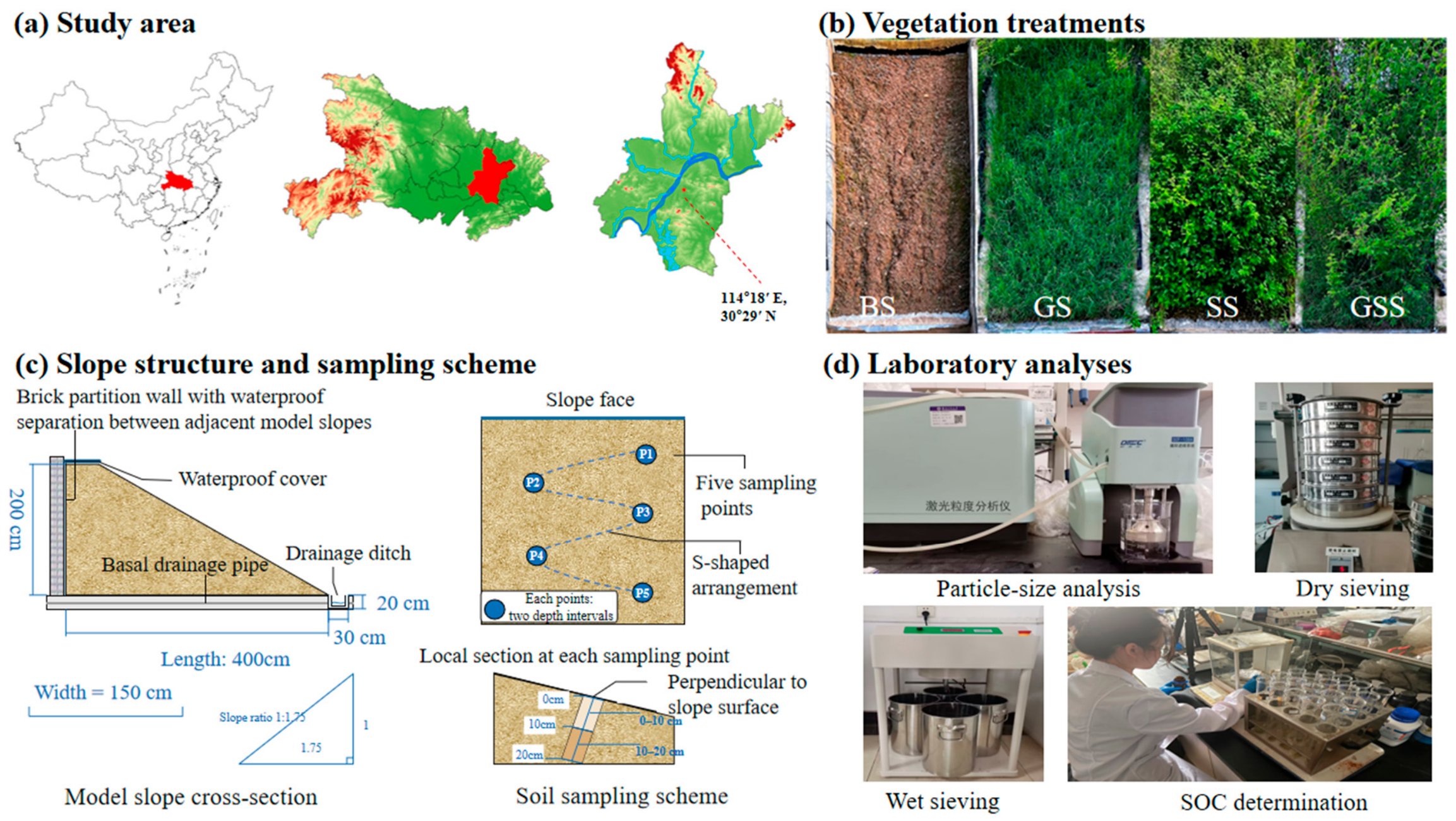
The experimental site is located in Wuhan, Hubei Province, Central China (114°18′ E, 30°29′ N), at an elevation of approximately 30 m. The region has a humid northern subtropical monsoon climate, with a mean annual temperature of 15.8–17.5 °C and mean annual precipitation of approximately 1284.5 mm. To simulate field conditions, four model slopes, each measuring 400 cm (length) × 150 cm (width) × 200 cm (height), were constructed in June 2020 at the field test base of the Key Laboratory of River and Lake Health Smart Perception and Ecological Restoration, Ministry of Education, Hubei University of Technology [29], as shown in Figure 1. The slope ratio was 1:1.75. The fill soil used for all four model slopes was collected from the same cut slope in Wuhan City, Hubei Province. According to the USDA soil texture classification system, the collected soil was classified as silt loam based on its particle-size distribution. A formal soil taxonomic classification under the World Reference Base for Soil Resources (WRB) was not determined for the source soil. The available records did not include the soil-profile descriptions and diagnostic information required for a reliable taxonomic classification. Before filling, the soil was air-dried, crushed, cleaned of visible debris, sieved, and thoroughly mixed to improve the homogeneity of the fill material. The initial water content of the fill soil was approximately 15.6%. The model slopes were constructed in successive 5 cm layers. The target dry density was approximately 1.49 g cm⁻³, corresponding to 85% of the maximum dry density (1.75 g cm⁻³). The required soil mass for each layer was determined from the designed layer volume and the target dry density. The soil for each layer was spread uniformly and manually compacted to the designed compacted thickness of 5 cm. Compaction was controlled primarily through the predetermined soil mass, layer volume, target dry density, and designed compacted thickness, rather than a prescribed number of passes. The same filling and compaction procedure was applied to all four model slopes. The exact number of compaction passes and the specific model of the compaction tool were not retained in the experimental records. After filling, the slopes were watered to facilitate soil settlement before vegetation establishment. The horizontal surface at the top of each model slope was covered with waterproof material to prevent direct rainfall infiltration from the slope crest. A basal drainage pipe was installed at the base of the model slopes to facilitate subsurface drainage. A drainage ditch measuring 30 cm in width and 20 cm in depth was installed at the toe of each model slope. Surface runoff was conveyed to the toe drainage ditch and discharged directly from the experimental system. Runoff was not collected or quantified. Adjacent model slopes were separated by brick partition walls and waterproof material to minimize lateral hydraulic interference. The basic physical properties of the common fill material are presented in Table 1. These values do not constitute slope-specific baseline measurements. No slope-specific baseline measurements were available before vegetation establishment; therefore, initial equivalence among the four model slopes was not independently demonstrated.

Figure 1. Study area location and experimental setup of the model slopes, vegetation treatments, soil sampling scheme, and laboratory analyses. BS, bare slope; GS, grass treatment planted with Cynodon dactylon; SS, shrub treatment planted with Magnolia multiflora; GSS, grass–shrub treatment planted with C. dactylon and M. multiflora; SOC, soil organic carbon. The P1–P5 arrangement shown in (c) is schematic and not to scale.

Table 1. Basic physical parameters of the soil used to fill model slopes.

Initial Water Content	Optimum Water Content	Maximum Dry Density	Natural Dry Density	Plastic Limit	Liquid Limit
15.6%	20%	1.75 g·cm−3	1.5 g·cm−3	23%	41%

In Central China, Cynodon dactylon and Magnolia multiflora are widely distributed and commonly used for slope restoration. Accordingly, three vegetation treatments were established: grass treatment (GS) seeded with C. dactylon, shrub treatment (SS) seeded with M. multiflora, and grass–shrub treatment (GSS) seeded with a 1:1 mixture of the two species. A bare slope (BS) with the same dimensions served as the control. Vegetation was established by direct seeding in June 2020. The seeding density was 30 g m⁻² for GS and SS, while the total seeding density for GSS was 30 g m⁻², with the two species mixed at a 1:1 ratio. The basic characteristics of the four model slopes are presented in Table 2.

Table 2. Model slope design.

Vegetation Treatment	Slope Ratio	Vegetation Configuration	Seeding Density
BS	1:1.75	-	-
GS	1:1.75	Cynodon dactylon	30 g/m2
SS	1:1.75	Magnolia multiflora	30 g/m2
GSS	1:1.75	Cynodon dactylon and Magnolia multiflora	30 g/m2

All four model slopes were located within the same open experimental site and had the same orientation and aspect, thereby receiving comparable natural rainfall and solar exposure. During the two-year vegetation establishment period, all four model slopes, including BS, received irrigation and fertilization according to the same general management principles. Irrigation was applied as needed, mainly during early vegetation establishment and subsequent dry periods, rather than on a fixed schedule. In the vegetated treatments, mowing or trimming was performed as needed when vegetation growth became excessive or maintenance was required. Replanting or reseeding was undertaken as needed where vegetation establishment was insufficient or plants were missing. For the bare-slope treatment, spontaneously established vegetation was manually removed to maintain the bare-slope condition. Detailed treatment-specific records of irrigation and fertilization timing, frequency, and amounts, and of fertilizer type, were not retained. Records of the dates and numbers of mowing/trimming and replanting/reseeding operations were also not retained.

2.2. Soil Sampling

Soil sampling was conducted in October (autumn), approximately two years after vegetation establishment. All four model slopes were sampled on the same day. Five sampling locations (P1–P5) were selected within each model slope using an S-shaped sampling pattern. Exact coordinates and distances from the crest, toe, and lateral boundaries were not recorded. No rainfall occurred, and no artificial irrigation was applied to any of the four model slopes during the seven consecutive days preceding sampling. A separate pre-sampling soil-moisture record was available for BS, but its sampling depth, location, and replication details could not be confirmed. Corresponding pre-sampling records were not available for GS, SS, or GSS. At each sampling location, soil samples were collected from the 0–10 cm and 10–20 cm layers along a direction perpendicular to the slope surface. Before sampling, the aboveground vegetation at each sampling location was carefully cut with scissors to expose the soil surface, and surface litter and visible plant residues were removed with minimal disturbance to the underlying soil.

For soil aggregate analysis, soil collected from the five sampling locations within the same soil layer was combined to form a composite sample of approximately 1 kg. The samples were placed in rigid plastic containers and transported to the laboratory to minimize disturbance of the original soil structure. Visible stones, roots, and plant residues were manually removed. The samples were naturally air-dried under ventilated laboratory conditions and gently broken into approximately 10 mm aggregates before aggregate-size analysis.

For SOC and SOM determination, soil collected from the five sampling locations within each soil layer was combined and stored in sealed plastic bags. After visible stones and roots were removed, the samples were air-dried, ground, and sieved before chemical analysis. For pH determination, soil collected from P1–P5 within each model slope and soil depth was combined to form one composite sample. For particle-size analysis, soil collected from P1–P5 within each model slope and soil depth was combined to form one composite sample before analysis.

For the determination of soil bulk density, soil water content, total porosity, and field capacity, undisturbed soil samples were collected separately from the 0–10 cm and 10–20 cm layers at each of the five sampling locations using 100 cm³ cutting rings. The five sampling locations within each model slope represented within-slope subsamples rather than independent replicates of the vegetation treatment.

2.3. Laboratory Analysis

The initial water content, natural dry density, liquid limit, plastic limit, maximum dry density, and optimum water content of the fill soil were determined according to the Standard for Geotechnical Testing Method (GB/T 50123-2019). Water content was determined by the oven-drying method, density by the cutting-ring method, liquid and plastic limits by the liquid–plastic limit test, and maximum dry density and optimum water content by the compaction test. Soil bulk density, soil water content, total porosity, and field capacity were determined using undisturbed soil samples collected with 100 cm³ cutting rings [30]. The cutting-ring samples were weighed under field-moist conditions and then immersed in water for 12 h, with the water level maintained at the upper edge of the rings. After saturation, the samples were weighed and subsequently oven-dried at 110 °C to constant mass. Soil bulk density was calculated as the oven-dry soil mass divided by the cutting-ring volume, while soil water content, total porosity, and field capacity were calculated from the corresponding field-moist, saturated, and oven-dry masses. Soil pH was determined potentiometrically according to HJ 962-2018 at a soil-to-water ratio of 1:2.5 using a PHSJ-3E pH meter (Shanghai INESA Scientific Instrument Co., Ltd., Shanghai, China) [31]. The content of aggregates with different particle sizes was determined using dry and wet sieving methods [32]. Soil organic carbon (SOC) was determined using the potassium dichromate oxidation method [33]. Soil organic matter (SOM) was subsequently calculated from SOC using a conversion factor of 1.724 (SOM = SOC × 1.724). Both SOC and SOM were expressed as percentages of soil dry mass [33]. Soil particle-size distribution was determined using an LT3600 Plus laser particle-size analyzer(Linkoptik Instruments Co., Ltd., Zhuhai, China). Before measurement, the soil samples were air-dried, ground, cleared of visible roots, stones, and other debris, and sieved. No additional chemical pretreatment for the removal of organic matter or carbonates was applied.

The dry-sieving procedure was conducted as follows. Visible stones, plant residues, and roots were first removed manually. The air-dried soil samples were gently broken into approximately 10 mm aggregates to minimize artificial breakage. Then, a 200 g subsample was placed in a sieve stack with aperture sizes of 5, 3, 2, 1, 0.5, and 0.25 mm and mechanically sieved for 10 min. Seven aggregate-size fractions were obtained: >5 mm, 3–5 mm, 2–3 mm, 1–2 mm, 0.5–1 mm, 0.25–0.5 mm, and <0.25 mm. Each fraction was collected and weighed separately. A 200 g sample mass was used to obtain a representative initial aggregate-size distribution and to provide sufficient material for the determination of individual aggregate fractions.

For wet sieving, a 50 g subsample was proportionally reconstructed according to the mass distribution of the aggregate-size fractions obtained by dry sieving. This procedure preserved the representative initial aggregate-size distribution while reducing excessive sample accumulation, sieve clogging, and overloading during wet sieving. The reconstructed sample was placed in a sieve stack with aperture sizes of 5, 3, 2, 1, 0.5, and 0.25 mm using a MINC-100 soil aggregate analyzer (Mince Instrument Equipment (Xiamen) Co., Ltd., Xiamen, China). The sample was prewetted in water for 5 min and subsequently oscillated at 30 oscillations min⁻¹ with an amplitude of 4 cm for 30 min. After wet sieving, the aggregates retained on each sieve were carefully transferred into aluminum containers, oven-dried at 105 °C to constant mass, and weighed.

The mean weight diameter (MWD), geometric mean diameter (GMD), percentage of aggregate destruction (PAD), water-stable aggregate content (WSA), and soil erodibility factor (K) were used to characterize aggregate stability [24,34,35,36]. Larger MWD, GMD, and WSA values and lower PAD and K values indicate greater aggregate stability. For the calculation of MWD and GMD, the representative diameters of the >5, 3–5, 2–3, 1–2, 0.5–1, 0.25–0.5, and <0.25 mm aggregate classes were 6.5, 4.0, 2.5, 1.5, 0.75, 0.375, and 0.15 mm, respectively. W_i represents the mass fraction of each aggregate-size class (dimensionless, 0–1). MWD and GMD were calculated separately for dry-sieved and water-stable aggregates; for water-stable aggregates, the calculation was based on the six fractions retained above 0.25 mm.

The MWD is an important parameter describing particle size distribution of aggregates. It can be computed by Equation (1) [24,35].

$$\mathit{MWD}=\sum _{i=1}^n\left(W_i{X}_i\right)$$

(1)

where X_i is the representative diameter of the ith aggregate-size class (mm), W_i is the mass fraction of the ith aggregate-size class (dimensionless, 0–1), and n is the number of aggregate-size classes. The representative diameters of the >5, 3–5, 2–3, 1–2, 0.5–1, 0.25–0.5, and <0.25 mm classes were 6.5, 4.0, 2.5, 1.5, 0.75, 0.375, and 0.15 mm, respectively.

The GMD describes the particle size distribution of aggregates, which is calculated by Equation (2) [24,35].

$$\mathit{GMD}=\exp \left[\frac{{\displaystyle \sum _{i=1}^n}(W_i\ln R_i)}{{\displaystyle \sum _{i=1}^n}{W}_i}\right]$$

(2)

where R_i is the representative diameter of the ith aggregate-size class (mm), and W_i is the corresponding mass fraction (dimensionless, 0–1). MWD and GMD were calculated separately for dry-sieved and water-stable aggregates. For water-stable aggregates, the calculations were based on the six fractions retained above 0.25 mm.

The percentage of aggregate destruction (PAD) reflects the degree of aggregate breakdown under water action. Lower PAD values indicate greater aggregate stability. PAD was calculated using Equation (3) [24,34].

$$PAD={\displaystyle \frac{W_{d>0.25}-W_{w>0.25}}{W_{d>0.25}}}\times 100\%$$

(3)

where W_d>0.25 and W_w>0.25 represent the >0.25 mm aggregates in dry and wet sieving, respectively, %.

Accordingly, the mass proportion of water-stable aggregate (WSA) could be calculated by Equation (4) [24,36].

$$WSA={\displaystyle \frac{{\displaystyle {\sum }_{i=1}^n{m}_i}}{\mathrm{m}}}\times 100\%$$

(4)

where m_i is the mass of ith water-stable aggregate fraction >0.25 mm, g; and m is the total initial mass of the soil sample used for wet sieving, g.

The soil erodibility factor (K) reflects the susceptibility of soil to erosion and was calculated using Equation (5) [35].

$$K=7.954\times \left\{0.0017+0.0494\times \exp \left[-0.5\times {\left({\displaystyle \frac{\lg GMD+1.675}{0.6986}}\right)}^2\right]\right\}$$

(5)

Each laboratory determination was performed in triplicate, and the mean value of the three analytical replicates was used for subsequent calculations.

2.4. Data Analysis

Data were organized and preliminarily processed using Excel 2021. Each vegetation treatment was represented by one model slope, which constituted the experimental unit. The five cutting-ring samples collected within each model slope and soil depth were within-slope subsamples and were not independent vegetation-treatment replicates.

For pH, SOC, and SOM, the reported means and standard deviations (SDs) were based on triplicate analytical measurements of one composite sample per model slope and soil depth (n = 3 analytical measurements). These SDs represent analytical variability. For soil bulk density, soil water content, total porosity, and field capacity, the value reported for each model slope and soil depth was the arithmetic mean of the five within-slope cutting-ring subsamples (n = 5), and the corresponding SD describes variability among those five subsamples.

Because the four vegetation treatments were not independently replicated at the model-slope level, inferential statistical tests were not used to compare BS, GS, SS, and GSS or to test vegetation treatment × soil depth interactions. Therefore, no post hoc multiple-comparison tests were performed, and differences among vegetation treatments and soil depths were described descriptively. Values reported for the 0–20 cm soil layer were calculated as the arithmetic mean of the corresponding values for the 0–10 and 10–20 cm layers.

Exploratory Pearson correlation analysis was performed using SPSS 16.0 to describe associations among soil physicochemical properties, aggregate-size fractions, and aggregate stability indicators. The analysis used one 0–20 cm mean value for each of the four model slopes, one per vegetation treatment (n = 4). Only Pearson correlation coefficients (r) are reported. Given the four observations, interpretation is limited to descriptive, exploratory associations and does not establish causal relationships. All figures were prepared using Origin 2021.

3. Results and Analysis

3.1. Soil Physicochemical Properties

Differences in soil properties were observed among different vegetation treatments (Table 3). Vertically, the soil bulk density gradually declined along with the increasing depth. Among the four vegetation treatments, the soil bulk density was ranked as GSS < SS < GS < BS, and the mean value of the three vegetated treatments was approximately 7.1% lower than that of BS. The total porosity was ranked as SS (45.47%) < GS (47.33%) < BS (48.75%) < GSS (49.00%). Moreover, the porosity of the topsoil was higher than that of the sublayer in SS and GSS, whereas the opposite pattern was observed in GS and BS. As for the soil water retention capacity, differences could be found among the four vegetation treatments. In the 0–20 cm soil layer, the soil water content in GSS (28.41%) and GS (24.23%) was higher than that in BS (22.99%) and SS (21.98%). The field capacity was also the highest in GSS (21.84%), followed by BS (19.72%), GS (19.45%), and SS (18.89%). The GSS had the highest observed soil water content and field capacity among the four model slopes. Vertically, the soil water content in all four treatments showed 0–10 cm < 10–20 cm. The field capacity showed 0–10 cm > 10–20 cm in SS and GSS, but 0–10 cm < 10–20 cm in GS and BS.

Table 3. Soil physicochemical properties under different vegetation treatments and soil depths.

Vegetation Treatment	Depth /cm	Bulk Density /g·cm−3	Porosity /%	Water Content /%	Field Capacity /%	pH	SOC (%)	SOM (%)
SS	0–10	1.44 ± 0.03	46.39 ± 0.61	21.70 ± 0.53	19.20 ± 0.73	7.99 ± 0.05	3.056 ± 0.125	5.269 ± 0.216
	10–20	1.42 ± 0.02	44.54 ± 0.73	22.26 ± 0.57	18.57 ± 0.83	7.75 ± 0.04	1.527 ± 0.134	2.633 ± 0.231
GS	0–10	1.49 ± 0.03	44.96 ± 1.12	24.16 ± 1.03	18.27 ± 0.65	8.18 ± 0.03	3.572 ± 0.241	6.158 ± 0.415
	10–20	1.47 ± 0.03	49.70 ± 1.24	24.29 ± 0.95	20.63 ± 0.72	7.92 ±0.06	1.481 ± 0.071	2.55 ± 0.122
GSS	0–10	1.28 ± 0.01	49.49 ± 1.76	27.87 ± 1.56	21.96 ± 1.12	8.21 ± 0.08	4.023 ± 0.155	6.936 ± 0.267
	10–20	1.26 ± 0.02	48.51 ± 1.84	28.94 ± 1.37	21.72 ± 1.08	8.11 ± 0.09	2.396 ± 0.120	4.131 ± 0.207
BS	0–10	1.51 ± 0.04	48.51 ± 0.91	22.69 ± 1.24	19.55 ± 0.93	8.24 ± 0.11	2.071 ± 0.110	3.570 ± 0.190
	10–20	1.49 ± 0.03	48.98 ± 0.58	23.29 ± 1.37	19.88 ± 0.62	8.19 ± 0.13	1.057 ± 0.080	1.822 ± 0.137 1

¹ Values are presented as arithmetic mean ± standard deviation (SD). For pH, SOC, and SOM, the means and SDs are based on triplicate analytical measurements of one composite sample per model slope and soil depth (n = 3 analytical measurements); these SDs represent analytical variability. For soil bulk density, soil water content, total porosity, and field capacity, the means and SDs are based on five within-slope cutting-ring subsamples per model slope and soil depth (n = 5 subsamples); these SDs represent variability among the five subsamples. The five subsamples are not independent vegetation-treatment replicates. SOC and SOM are expressed as percentages of soil dry mass.

The soil pH ranged from 7.75 to 8.24 among the four vegetation treatments. The highest pH value was observed in BS(8.22). The vegetated treatments generally showed lower pH values than BS. The vegetated treatments generally showed lower pH values than BS. SOC and SOM also differed among the vegetation treatments. In the 0–20 cm soil layer, the SOC was ranked as BS(1.564%) < SS(2.292%) < GS(2.527%) < GSS(3.210%). The SOM was ranked as BS(2.696%) < SS(3.951%) < GS(4.357%) < GSS(5.534%). Compared with BS, the mean SOC and SOM contents of the three vegetated treatments were approximately 71.1% higher. These percentages were calculated using the mean values of SS, GS, and GSS relative to BS. Vertically, both SOC and SOM in four slopes presented topsoil > sublayer soil. The differences of SOC between the two layers in BS, GS, SS, GSS were 1.014, 2.091, 1.529, and 1.627, respectively, and that of SOM in the four slopes were 1.748, 3.605, 2.636, and 2.805, respectively. The SOC and SOM contents and their depth-related patterns differed among vegetation treatments.

3.2. Soil Particle-Size Distribution

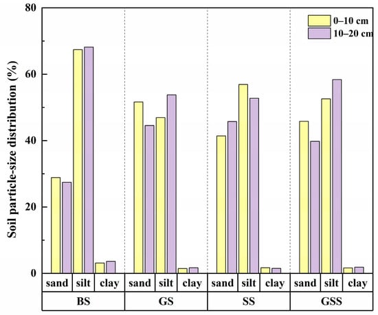
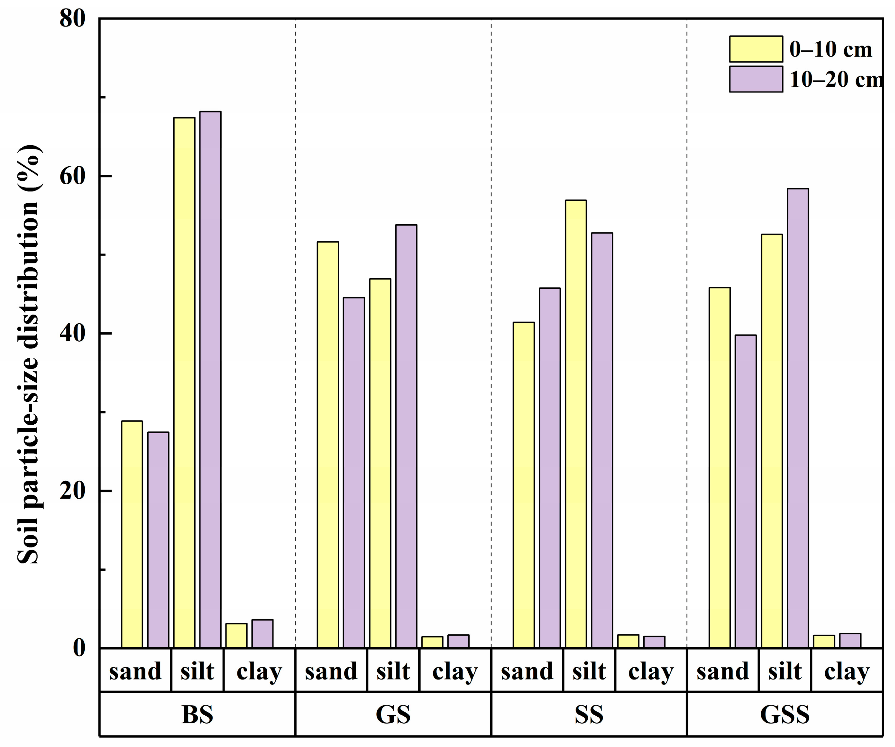
The soil particle-size distribution affects aggregate stability, permeability, and fertility. It is mainly divided into the following categories: sand (0.050~2.000 mm), silt (0.002~0.050 mm), and clay (≤0.002 mm). The proportions of soil particles differed among the four vegetation treatments (Figure 2). After two years of vegetation establishment, the vegetated treatments generally had lower silt and clay contents and higher sand contents than BS. In the 0–20 cm soil layer, all four slope soils presented silt > sand > clay. Among them, the silt content was higher than 50%, and ranked as BS(67.785%) > GSS(55.473%) > SS(54.822%) > GS(50.358%). The clay content ranged from 1.564% to 3.359%, and was ranked as BS(3.359%) > GSS (1.737%) > SS(1.602%) > GS(1.564%). Vertically, the sand content in GS, GSS, and BS showed 0–10 cm > 10–20 cm, whereas the silt content showed 0–10 cm < 10–20 cm. In SS, the sand and silt fractions showed the opposite vertical patterns.

Figure 2. Soil particle-size distribution under different vegetation treatments and soil depths.

3.3. Soil Aggregate-Size Distribution

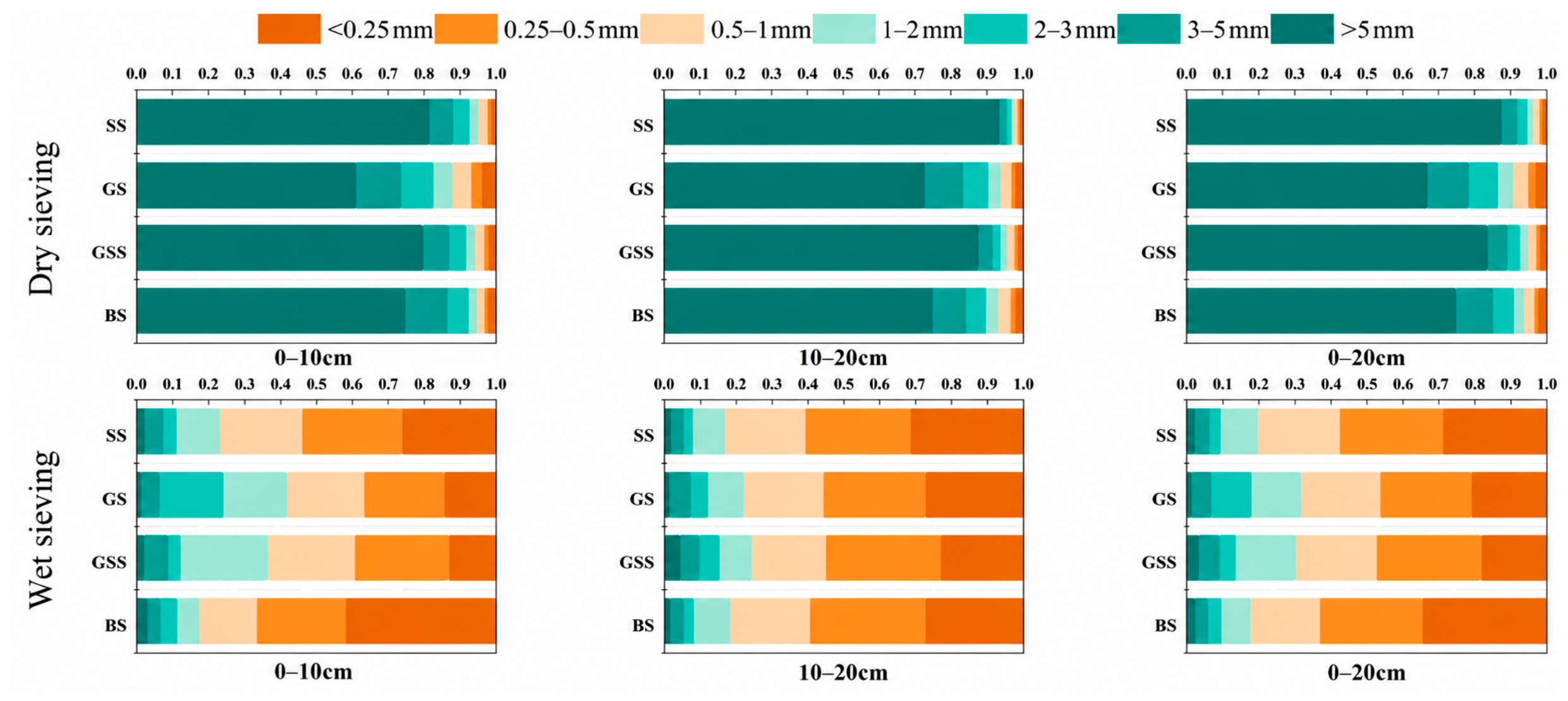
Figure 3 presents the size distribution of soil aggregates derived by dry and wet sieving. Overall, the non-water-stable and water-stable aggregates were divided into seven fractions and showed differences among the four vegetation treatments. As the size grade increased, the non-water-stable aggregates gradually decreased, while the water-stable aggregates increased. Under dry sieving conditions, the >5 mm aggregates in SS (175.53 g) and GSS (167.67 g) were higher than that in BS (148.51 g). Although the >5 mm fraction in GS (134.13 g) was slightly lower than that in BS, the 2–5 mm fraction increased. As for wet sieving, the content of water-stable aggregates was GSS(40.98 g) > GS(39.59 g) > SS(35.65 g) > BS(32.73 g). The >1 mm aggregates showed GS(15.86 g) > GSS(15.15 g) > SS(9.92 g) > BS(8.83 g). In the 0–20 cm layer, the vegetated treatments showed higher water-stable aggregate contents than BS. The grass treatment showed a higher water-stable aggregate content than the shrub treatment. The proportions of the 1–0.5 mm and 0.5–0.25 mm fractions exceeded 40%, which were dominant in water-stable aggregates. The >5 mm and 3–5 mm fractions accounted for 1.23–4.4% and 3.41–6.63%, respectively, and their contents were relatively stable. Comparably, variations were observed in the 2–3 mm and 1–2 mm fractions. In the 2–3 mm fraction, GSS and GS contained relatively more water-stable aggregates than SS and BS. In the 1–2 mm fraction, the order of water-stable aggregate content was GSS(8.39 g) > GS(6.90 g) > SS(5.25 g) > BS(4.08 g). GSS showed the highest content of the 1–2 mm water-stable aggregate fraction among the four vegetation treatments (Figure 3).

Figure 3. Proportion of aggregate size distribution derived by dry and wet sieving under different vegetation treatment.

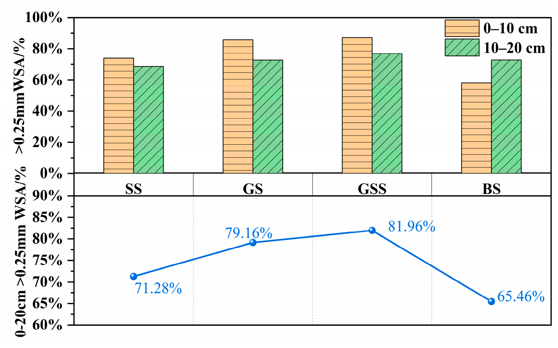
Generally, >0.25 mm aggregates are considered macroaggregates, while <0.25 mm aggregates are referred to as microaggregates. The WSA of the four vegetation treatments differed from each other (Figure 4). In the overall 0–20 cm layer, the WSA presented GSS (81.96%) > GS (79.16%) >SS (71.28%) > BS (65.46%). In the 0–10 cm layer, the WSA was ranked as GSS (86.98%) > GS (85.60%) > SS (73.94%) > BS (58.18%). In the 10–20 cm layer, such differences narrowed, with WSA ranging from 68.62% to 76.94%. The WSA of BS presented topsoil < sublayer soil, whereas the opposite pattern was observed in the three vegetated treatments. In the 0–10 cm layer, the three vegetated treatments showed higher WSA values than BS (Figure 4). Notably, the WSA of GSS was higher than that of the other three vegetation treatments in the 0–10 cm, 10–20 cm, and overall 0–20 cm soil layers.

Figure 4. Comparison of WSA associated with different vegetation treatments.

3.4. Soil Aggregate Stability Indicators

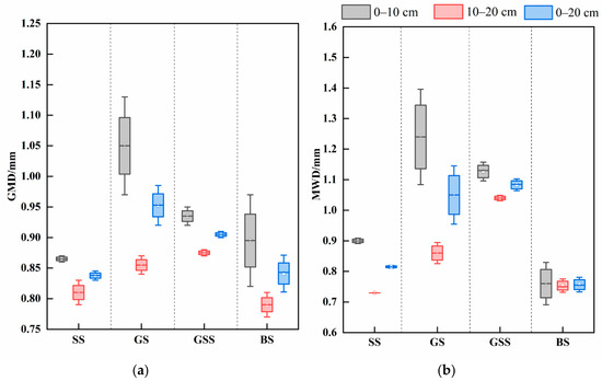
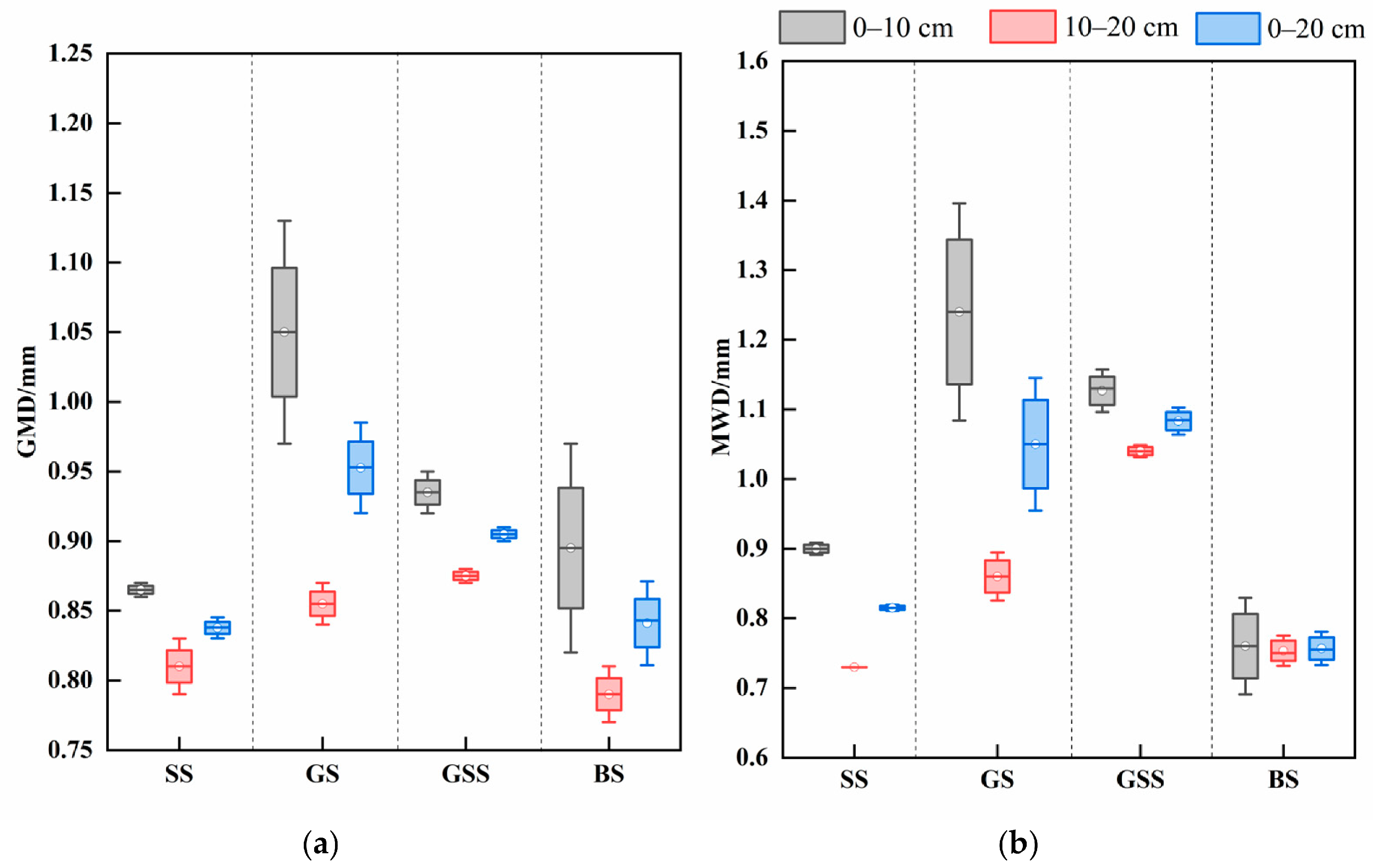
Figure 5 shows the results of GMD and MWD associated with different vegetation treatments and soil depths. In the 0–10 cm layer, GMD followed GS > GSS > BS > SS, whereas MWD followed GS > GSS > SS > BS. In the 10–20 cm layer, GMD followed GSS > GS > SS > BS, whereas MWD followed GSS > GS > BS > SS. In the overall 0–20 cm layer, GS had the highest GMD (0.952 mm), followed by GSS (0.905 mm), BS (0.839 mm), and SS (0.836 mm). MWD was highest in GSS (1.085 mm), followed by GS (1.049 mm), SS (0.815 mm), and BS (0.756 mm). It was worth noting that the differences in GMD and MWD between the two soil layers were relatively large in GS, especially for the 0–10 cm layer. The smallest difference between the two soil layers occurred in SS for GMD and in BS for MWD.

Figure 5. Comparison of GMD and MWD associated with different vegetation treatment and soil depths: (a) GMD; and (b) MWD.

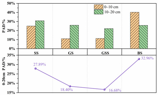
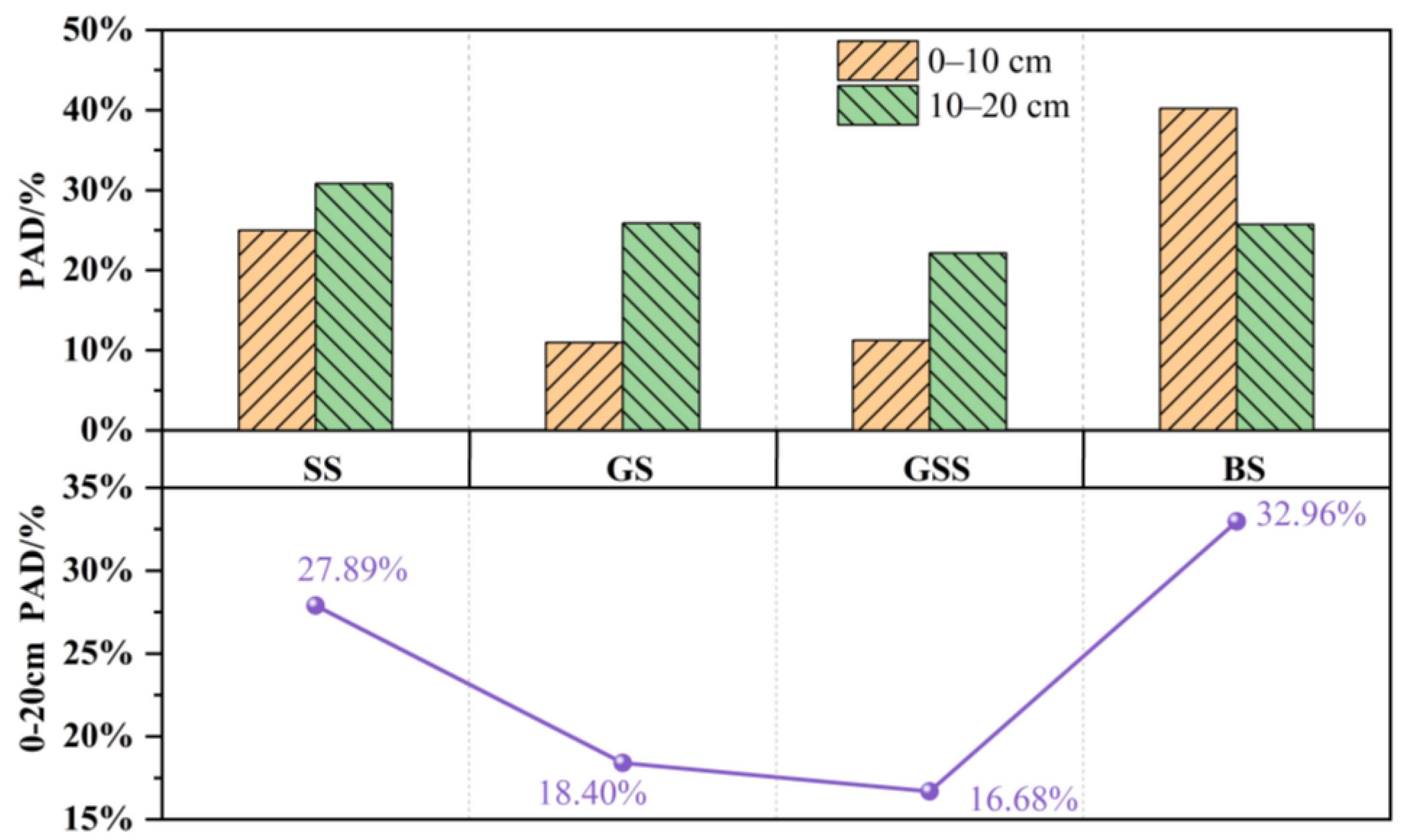
In the 0–20 cm layer, all three vegetated treatments had lower PAD than BS (Figure 6). In the 0–20 cm layer, PAD followed BS (32.96%) > SS (27.89%) > GS (18.40%) > GSS (16.68%). The mean PAD of SS, GS, and GSS was 36.31% lower than BS. The differences from BS were more pronounced in the 0–10 cm layer, where PAD was 24.96% in SS, 10.95% in GS, 11.24% in GSS, and 40.20% in BS. In the 10–20 cm layer, PAD was 30.81% in SS, 25.86% in GS, 22.13% in GSS, and 25.72% in BS. GSS had the lowest PAD, whereas SS and GS had a higher PAD than BS. GSS had the lowest PAD in the 0–20 cm layer.

Figure 6. Variation characteristics of PAD associated with different vegetation treatment and soil depths.

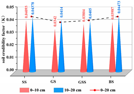
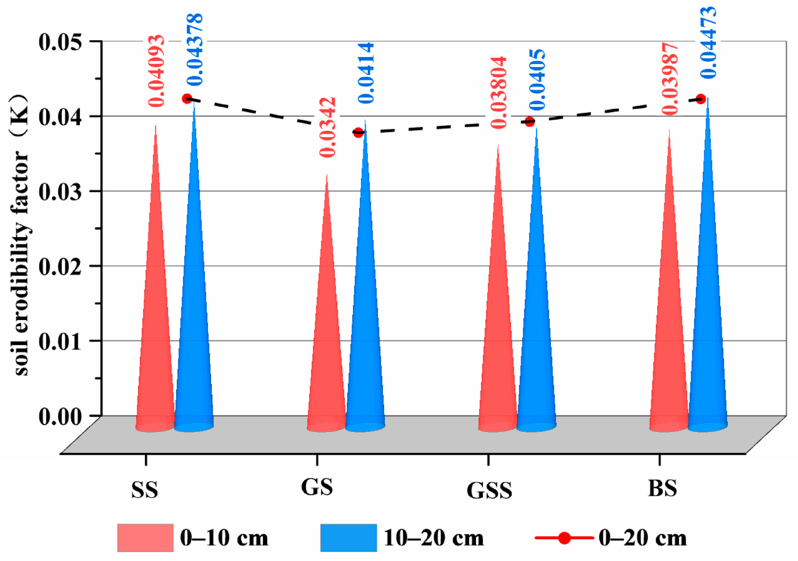
Figure 7 compares the K values among the four vegetation treatments. In the 0–20 cm layer, K was 0.04235 in SS, 0.04230 in BS, 0.03927 in GSS, and 0.03780 in GS, following SS > BS > GSS > GS. Vertically, K also differed between the two soil layers. In the 0–10 cm layer, K ranged from 0.03420 in GS to 0.04093 in SS, with values of 0.03804 in GSS and 0.03987 in BS. The differences of K in the 10–20 cm layer decreased. In the 10–20 cm layer, K was 0.04378 in SS, 0.04140 in GS, 0.04050 in GSS, and 0.04473 in BS. Overall, K increased with soil depth in all four vegetation treatments. The topsoil (0–10 cm) therefore showed a lower erodibility than the sublayer (10–20 cm). In the 0–20 cm layer, GS had the lowest K, followed by GSS. The mean K of SS, GS, and GSS was 5.90% lower than BS. In conclusion, GS and GSS showed a lower soil erodibility than SS.

Figure 7. Comparison of K associated with different vegetation treatment and soil depths.

3.5. Results of Exploratory Pearson Correlation Analysis

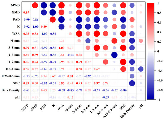
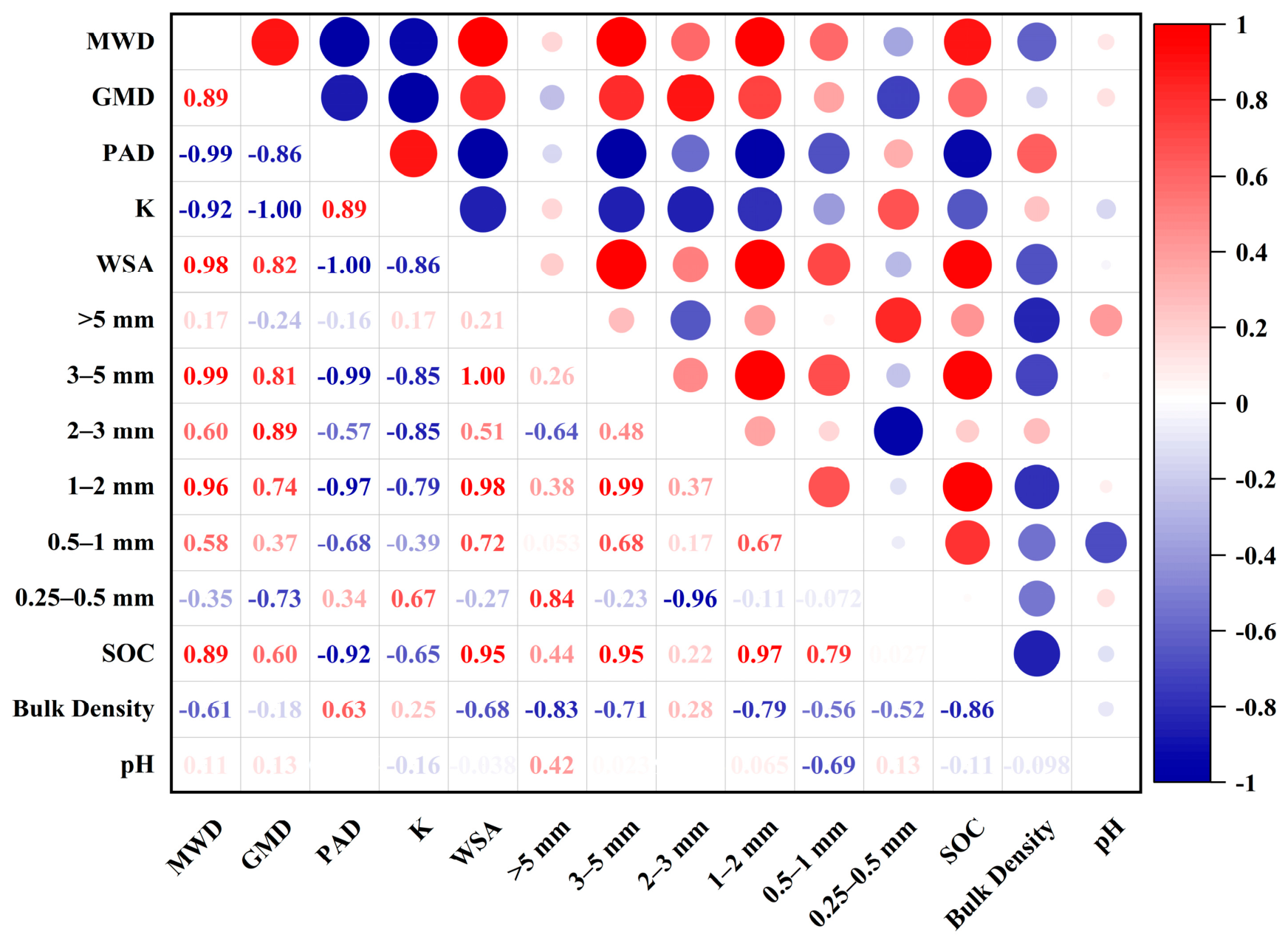
An exploratory Pearson correlation analysis of the 0–20 cm values from the four model slopes (n = 4) gave negative coefficients between the soil bulk density and MWD (r = −0.605), GMD (r = −0.179), and WSA (r = −0.679), and positive coefficients with PAD (r = 0.626) and K (r = 0.251) (Figure 8). For the 3–5 mm aggregate fraction, the coefficients with MWD, WSA, and PAD were 0.986, 0.998, and −0.994, respectively; the corresponding coefficients for the 1–2 mm fraction were 0.965, 0.983, and −0.972. The coefficients between soil pH and the five aggregate stability indicators ranged from −0.167 to 0.132. The coefficients between SOC and the 3–5 mm and 1–2 mm aggregate fractions were 0.953 and 0.973, respectively. Because SOM was calculated from SOC using a conversion factor of 1.724, only SOC was retained in the revised correlation analysis to avoid redundancy. The interpretation of these coefficients is limited to descriptive, exploratory associations among the four model slopes.

Figure 8. Exploratory Pearson correlation matrix among soil properties, aggregate-size fractions, and soil aggregate stability indicators. The analysis used the 0–20 cm mean values of the four model slopes, one per vegetation treatment (n = 4). Only Pearson correlation coefficients (r) are reported, and interpretation is limited to descriptive, exploratory associations. Red and blue indicate positive and negative coefficients, respectively, and circle size represents the absolute value of r. Values in the lower triangle represent r. MWD, mean weight diameter; GMD, geometric mean diameter; PAD, percentage of aggregate destruction; WSA, water-stable aggregate content; K, soil erodibility factor; SOC, soil organic carbon.

4. Discussion

4.1. Effect of Vegetation Configuration on Soil Physicochemical Properties

Due to the combined effects of climate, plant litter, and roots, soil physicochemical properties show vertical variation, which further affects the erosion resistance capacity at different depths. Soil bulk density represents its compaction degree. The lower the soil bulk density, the looser the soil texture, the better the porosity, and the stronger the aeration and water permeability [9]. These have positive impacts on enhancing the soil anti-erosion capacity. The soil particle arrangement and pore structure affect the water retention characteristics and SOC content, thereby altering soil erodibility [26]. Recent studies have also shown that erosion-related differences in soil moisture, density-related properties, porosity, and particle-size distribution may vary with soil depth [37]. In this study, the vegetated treatments showed a lower soil bulk density than BS, and the soil bulk density was greater in the topsoil than in the sublayer (Table 3). This is consistent with the studies of Shellito et al. [38] and Ma et al. [5]. In addition, GSS exhibited the highest water content and total porosity, and the lowest bulk density (Table 3). Compared with GS and SS, the total porosity of GSS was 3.53% and 7.76% higher, respectively, while its soil bulk density was 14.19% and 11.19% lower, respectively. These differences cannot be attributed solely to the mixed vegetation treatment. Soil pH is a fundamental parameter of soil chemical properties [39]. In this study, the soil pH ranged from 7.75 to 8.24 (Table 3). Compared with BS, the pH values of GS, SS, and GSS were lower by 0.17, 0.35, and 0.06 pH units, respectively. The vegetated treatments generally showed a lower soil pH than BS. This may be related to organic compounds secreted by plant roots into the rhizosphere environment [40]. Vegetation restoration may alter the soil microenvironment and microbial activity, thereby affecting soil pH [41]. Herbaceous plants commonly have a higher coverage and more developed roots in the surface layer than shrubs. SOC and SOM are binding substances of soil aggregates, which can promote the formation of macroaggregates [42,43,44]. Therefore, high SOC and SOM contents are conducive to aggregate formation and soil aggregate stability. On the contrary, soil aggregates provide protective sites for SOC and SOM. The decomposition of microorganisms can be slowed down, which is beneficial for the stability and accumulation of SOC and SOM [36,45]. Therefore, the formation and transformation of soil aggregates are closely related to the process of soil carbon sequestration. In this study, SOC and SOM differed among vegetation treatments and soil depths, with both showing GSS > GS > SS > BS in the 0–20 cm layer. With depth, both SOC and SOM showed 0–10 cm > 10–20 cm (Table 3). This may partly reflect contributions from plant litter and dead roots. The higher SOC and SOM contents observed in GSS may partly reflect the differences in organic matter inputs associated with the mixed vegetation treatment [4,18].

4.2. Effect of Vegetation Configuration on Soil Aggregate Composition

The soil particle-size distribution determines the soil texture, porosity, and fertility, which, in turn, affect SOC, SOM, and plant growth. The soil used in this study was classified as silt loam according to the USDA soil textural classification, with sand particles (0.05–2 mm) accounting for 28.142%. Compared with BS, the vegetated treatments generally showed higher sand contents and lower silt and clay contents. Aggregate-size distributions also differed among the vegetation treatments in this study. The non-water-stable aggregates reflect the ability of soil aggregates to resist mechanical external forces, and the water-stable aggregates reflect soil stability characteristics. In this study, the >5 mm fractions in SS and GSS and the 2–5 mm fractions in GS were higher than those in BS (Figure 3). The dominant fractions of the wet-sieved aggregates in the vegetated treatments were 0.25–0.5 mm and 0.5–1 mm. Moreover, the soil aggregate stability is closely related to the proportion of >0.25 mm water-stable aggregates, namely, WSA, which was ranked as GSS (81.96%) > GS (79.16%) > SS (71.28%) > BS (65.46%) in this study (Figure 4). The higher 0–20 cm WSA values observed in the vegetated treatments relative to BS are consistent with the patterns reported by Fattet et al. [13], Li et al. [18], and Tang et al. [46]. This may be attributed to the fact that the formation of macroaggregates depends on the bonding effect of cementing materials produced by vegetation. The litters accumulating in surface soil would be decomposed by microorganisms to produce organic colloids such as humus and polysaccharides [47]. The roots also secrete organic acids, amino acids, and polysaccharides [48]. These materials can gather dispersed soil particles into macroaggregates through chemical bond and physical entanglement [40,48]. Meanwhile, the vegetated treatments showed a lower bulk density and differences in soil porosity compared with BS (Table 3). These changes may provide favorable conditions for microbial activity and organic matter decomposition, making it easier for microaggregates to cluster into macroaggregates [15,45]. On the other hand, plant canopies and litters significantly reduce water erosion [14]. Macroaggregates are less susceptible to destruction and thus accumulate in surface soil. It is worth noting that the WSA of GSS was higher than that of the other vegetation treatments (Figure 4). This difference may be related to the differences in litter inputs and root characteristics between grass and shrub, as suggested by previous studies. Previous studies have pointed out that the number of macroaggregates around the fibrous root system is significantly higher than in rootless areas [49]. Compared with Magnolia multiflora, Cynodon dactylon has a more developed fibrous root system, which may contribute to greater root-derived organic inputs according to previous studies. This may partly explain the higher macroaggregate contents observed in GS and GSS.

A major limitation of this study is that the initial equivalence among the four model slopes was not independently demonstrated because slope-specific baseline measurements were not obtained before vegetation establishment. The common soil source, thorough mixing, and common construction procedures were intended to improve initial comparability but did not establish equivalence. Therefore, the differences observed after two years are interpreted descriptively and cannot be attributed solely to vegetation treatments. Unmeasured initial between-slope variability cannot be excluded as a contributor to these differences. The lack of detailed management records is a methodological limitation and a potential source of confounding, as management-related effects cannot be completely separated from vegetation-treatment differences. The incomplete pre-sampling soil-moisture information limits the assessment of antecedent moisture differences among the model slopes and their possible influence on the water-related results.

4.3. Effect of Vegetation Configuration on Soil Aggregate Stability

GMD, MWD, PAD, and K are critical indicators reflecting soil aggregate stability. In this study, aggregate stability indicators differed descriptively among the four model slopes. For the 0–20 cm layer, the mean MWD and GMD of SS, GS, and GSS were 30.05% and 6.93% higher than BS, respectively, while their mean PAD and K were 36.31% and 5.90% lower, respectively (Figure 5, Figure 6 and Figure 7). For MWD and GMD, the vegetated mean was calculated as (SS + GS + GSS)/3, and the percentage increase relative to BS was calculated as [(vegetated mean − BS)/BS] × 100%, using unrounded values for the 0–20 cm layer. For PAD and K, the percentage reduction relative to BS was calculated as [(BS − vegetated mean)/BS] × 100%, using unrounded values for the 0–20 cm layer. This is consistent with most research findings of Peng et al. [50], Zhou et al. [24], and Zhang et al. [3]. As aforementioned, vegetation restoration may provide organic matter and enhance soil–root interactions. The increased SOC and SOM may contribute to the stabilization of soil particles. These processes may contribute to the greater stability and erosion resistance of surface soil aggregates on cut slopes. This study also found that soil aggregate stability and erosion resistance differed with soil depth, with the surface soil showing greater stability than the sublayer soil. As were indicated by the stability indicators; the GMD and MWD of all vegetated treatments showed 0–10 cm > 10–20 cm (Figure 5), while PAD and K showed 0–10 cm < 10–20 cm (Figure 6 and Figure 7). This may be related to more favorable litter, temperature, water, and oxygen conditions in surface soil. Such conditions may favor microbial activity and macroaggregate formation, thereby contributing to lower soil erodibility. Vegetation treatment is another factor associated with the distribution and stability of aggregates. In the 0–20 cm layer, GMD followed GS > GSS > SS, whereas MWD followed GSS > GS > SS among the three vegetated treatments. Moreover, GS and GSS showed relatively high SOM contents, while their pH values were lower than that of BS but higher than that of SS (Table 3). In the 0–20 cm layer, GS and GSS had a higher MWD and GMD and lower PAD and K than SS. Overall, grass showed better performance in soil physicochemical properties and erosion resistance than shrub. Compared with the single-plant treatments, the grass–shrub treatment corresponded to a higher total porosity, water content, SOC, and SOM, and lower bulk density (Table 3). This may be related to differences in root characteristics [40,51] and species diversity [52]. Vannoppen et al. [22] suggested that fibrous root systems are more effective than main root systems in erosion reduction. This is due to the fact that fibrous roots contact and bind more soil particles around them. Soil detachment can be considerably reduced by huge fibrous roots rather than the main root system [18]. Previous studies have reported contrasting root architectures between the two species: Cynodon dactylon develops a dense root system mainly distributed in shallow soil, whereas Magnolia multiflora is characterized by a thicker and longer main root with developed lateral roots [53]. Such differences in root traits may partly explain the higher SOC and SOM observed in GS and GSS, although root biomass and root secretions were not directly measured in this study. Differences in the canopy and root architecture between the two species may also contribute to the observed soil responses. These differences may partly explain the relatively lower aggregate stability observed in SS compared with GS and GSS. Mixed vegetation can enhance plant diversity and structural complexity. Liu et al. [49] found that the species diversity index is significantly positively correlated with soil quality. Bai et al. [52] also claimed that mixing plant with complementary ecological niches can improve both the mechanical and water stability of surface soil aggregates.

4.4. Exploratory Pearson Correlation Analysis of Soil Aggregate Stability

The exploratory Pearson correlation analysis describes associations among the four model slopes (n = 4), with the interpretation limited to descriptive patterns. In this study, the soil bulk density was negatively correlated with MWD, GMD, and WSA, and positively correlated with PAD and K (Figure 8). The coefficients for the 3–5 mm and 1–2 mm aggregate fractions were positive with MWD and WSA and negative with PAD (Figure 8). The coefficients between soil pH and the five aggregate stability indicators ranged from −0.167 to 0.132 within these four observations. Because SOM was calculated from SOC using a conversion factor of 1.724, only SOC was retained in the revised correlation analysis to avoid redundancy. SOC had positive coefficients with the 3–5 mm and 1–2 mm aggregate fractions (r = 0.953 and 0.973, respectively; Figure 8). Almeida et al. [54] and Zhou et al. [24] also reported that the SOC is closely related to 1–2 mm aggregates, MWD, K, and soil bulk density. These exploratory associations do not establish the mechanisms underlying aggregate formation or causal relationships among the measured variables. The contents of SOC and SOM also differed among vegetation treatments. Comparably, SOC and SOM were highest in the grass–shrub treatment (Table 3). As for aggregate stability indicators, the performance of the grass–shrub and grass treatments was almost the same. Overall, the grass–shrub and grass treatments showed a relatively favorable performance in soil aggregate stability.

5. Conclusions

This study descriptively compared the soil aggregate composition and stability among vegetation treatments two years after establishment. Because the initial equivalence among the four model slopes was not independently demonstrated, the observed differences cannot be attributed solely to vegetation treatments. The soil physicochemical properties, particle-size distribution, and stability indicators were successively analyzed. The correlations among soil properties, aggregate-size fractions, and aggregate stability indicators were also analyzed. Some main conclusions were drawn as follows:

(1)

The soil physicochemical properties differed among vegetation treatments and between the two soil layers. Compared with BS, the mean bulk density of the three vegetated treatments was approximately 7.1% lower, while the mean SOC and SOM contents were approximately 71.1% higher. Compared with BS, the pH values of GS, SS, and GSS were lower by 0.17, 0.35, and 0.06 pH units, respectively. Vertically, the soil water content was lower in the 0–10 cm layer than in the 10–20 cm layer for all treatments, whereas the bulk density, SOC, and SOM were higher in the 0–10 cm layer. The field capacity showed different depth-related patterns among treatments. Comparably, the grass–shrub treatment showed more favorable overall soil properties than the single-plant treatments.

(2)

Both the water-stable aggregate content and WSA followed GSS > GS > SS > BS. Vertically, the macroaggregate content and WSA were generally higher in the topsoil than in the sublayer soil. The vegetated treatments showed higher macroaggregate contents than BS, particularly in the 1–5 mm fractions. The grass treatment showed a higher water-stable aggregate content than the shrub treatment.

(3)

Aggregate stability indicators differed among the four model slopes. For the 0–20 cm layer, the mean MWD and GMD of SS, GS, and GSS were 30.05% and 6.93% higher than BS, respectively, while their mean PAD and K were 36.31% and 5.90% lower, respectively. In all three vegetated treatments, MWD and GMD were higher and PAD and K were lower in the 0–10 cm layer than in the 10–20 cm layer. GS had the highest GMD and lowest K, whereas GSS had the highest MWD and lowest PAD in the 0–20 cm layer.

(4)

An exploratory Pearson correlation analysis (n = 4) showed positive associations of the 3–5 mm and 1–2 mm aggregate fractions with MWD and WSA, negative associations with PAD, and positive associations of SOC with these fractions. The interpretation is limited to descriptive associations among the four model slopes and does not establish causality.

These findings provide experimental evidence for understanding the relationship between the vegetation configuration and soil aggregate stability on restored cut slopes. The results also provide a practical reference for vegetation selection in cut-slope restoration in Central China and other regions with comparable environmental and engineering conditions.

References

- Zhao, W.; Zhang, K.; Cen, Y.; Hu, W.; Yang, C.; Yang, Q. Response law and prediction model of soil erosion considering vegetation and litter cover under different rainfall intensities in the Loess Plateau. Soil Tillage Res. 2025, 251, 106559. [Google Scholar] [CrossRef] [Scilit]
- Hunakunti, A.; McBratney, A.B.; Minasny, B.; Field, D.J. Assessing soil erosion vulnerability using a novel capacity–condition framework (CCF): A case study from New South Wales, Australia. Int. Soil Water Conserv. Res. 2025, 13, 771–794. [Google Scholar] [CrossRef] [Scilit]
- Zhang, Y.; Li, P.; Liu, X.; Xiao, L. Changes in Soil Aggregate Fractions, Stability, and Associated Organic Carbon and Nitrogen in Different Land Use Types in the Loess Plateau, China. Sustainability 2022, 14, 3963. [Google Scholar] [CrossRef] [Scilit]
- Bora, M.J.; Bordoloi, S.; Pekkat, S.; Garg, A.; Sekharan, S.; Rakesh, R.R. Assessment of soil erosion models for predicting soil loss in cracked vegetated compacted surface layer. Acta Geophys. 2022, 70, 333–347. [Google Scholar] [CrossRef] [Scilit]
- Ma, R.; Hu, F.; Xu, C.; Liu, J.; Yu, Z.; Liu, G.; Zhao, S.; Zheng, F. Vegetation restoration enhances soil erosion resistance through decreasing the net repulsive force between soil particles. CATENA 2023, 226, 107085. [Google Scholar] [CrossRef] [Scilit]
- Xu, J.; Liu, M.; Yi, J.; Li, S.; Zhang, J.; Zhang, H. Influence of vegetation restoration strategies on seasonal soil water deficit in a subtropical hilly catchment of southwest China. CATENA 2025, 248, 108578. [Google Scholar] [CrossRef] [Scilit]
- Yan, Y.; Zhen, H.; Zhai, X.; Li, J.; Hu, W.; Ding, C.; Qi, Z.; Qiao, B.; Li, H.; Liu, X.; et al. The role of vegetation on earth bunds in mitigating soil erosion in Mollisols region of Northeast China. CATENA 2021, 196, 104927. [Google Scholar] [CrossRef] [Scilit]
- Chen, B.; Zhang, X. Effects of slope vegetation patterns on erosion sediment yield and hydraulic parameters in slope-gully system. Ecol. Indic. 2022, 145, 109723. [Google Scholar] [CrossRef] [Scilit]
- Ilek, A.; Kucza, J.; Szostek, M. The effect of the bulk density and the decomposition index of organic matter on the water storage capacity of the surface layers of forest soils. Geoderma 2017, 285, 27–34. [Google Scholar] [CrossRef] [Scilit]
- Mangalassery, S.; Sjögersten, S.; Sparkes, D.L.; Sturrock, C.J.; Mooney, S.J. The effect of soil aggregate size on pore structure and its consequence on emission of greenhouse gases. Soil Tillage Res. 2013, 132, 39–46. [Google Scholar] [CrossRef] [Scilit]
- Mikha, M.M.; Green, T.R.; Untiedt, T.J.; Hergret, G.W. Land management affects soil structural stability: Multi-index principal component analyses of treatment interactions. Soil Till Res. 2024, 235, 105890. [Google Scholar] [CrossRef] [Scilit]
- Wang, H.; Yue, C.; Mao, Q.; Zhao, J.; Ciais, P.; Li, W.; Yu, Q.; Mu, X. Vegetation and species impacts on soil organic carbon sequestration following ecological restoration over the Loess Plateau, China. Geoderma 2020, 371, 114389. [Google Scholar] [CrossRef] [Scilit]
- Fattet, M.; Fu, Y.; Ghestem, M.; Ma, W.; Foulonneau, M.; Nespoulous, J.; Le Bissonnais, Y.; Stokes, A. Effects of vegetation type on soil resistance to erosion: Relationship between aggregate stability and shear strength. CATENA 2011, 87, 60–69. [Google Scholar] [CrossRef] [Scilit]
- Liu, Y.; Wu, J.; Li, C. Model simulation of vegetation canopy precipitation interception in grassland ecosystems on the northeast margin of the Qinghai-Tibet Plateau. Ecol. Model. 2024, 488, 110576. [Google Scholar] [CrossRef] [Scilit]
- Yu, Z.; Zhang, J.; Zhang, C.; Xin, X.; Li, H. The coupling effects of soil organic matter and particle interaction forces on soil aggregate stability. Soil Tillage Res. 2017, 174, 251–260. [Google Scholar] [CrossRef] [Scilit]
- Zheng, J.; Zhang, J.; Ren, B.; Lin, H.; Li, Z.; Gu, F.; Zhu, B.; Harerimana, B.; Zhou, M. Soil aggregates, carbon and nitrogen content, and water retention across land uses in the Reshui River Catchment. Ecol. Eng. 2026, 222, 107807. [Google Scholar] [CrossRef] [Scilit]
- Ali, W.; Hussain, S.; Chen, J.; Hu, F.; Liu, J.; He, Y.; Yang, M. Cover crop root-derived organic carbon influences aggregate stability through soil internal forces in a clayey red soil. Geoderma 2023, 429, 116271. [Google Scholar] [CrossRef] [Scilit]
- Li, M.; Chen, X.W.; Leung, A.K. Grass species and mycorrhizal fungi improved aggregate stability of compacted and vegetated soils. Plant Soil 2025, 511, 1081–1099. [Google Scholar] [CrossRef] [Scilit]
- Zhao, Z.; Shi, P.; Niu, H.; Bai, L.; Cao, M.; Zu, P.; Li, Z. Response of soil organic carbon loss to runoff hydrodynamic parameters under vegetation and terracing measures on the Loess Plateau. CATENA 2025, 254, 108885. [Google Scholar] [CrossRef] [Scilit]
- Zhang, Y.; Zhen, Q.; Ma, W.; Jia, J.; Li, P.; Zhang, X. Dynamic responses of soil aggregate-associated organic carbon and nitrogen to different vegetation restoration patterns in an agro-pastoral ecotone in northern China. Ecol. Eng. 2023, 189, 106895. [Google Scholar] [CrossRef] [Scilit]
- Liu, G.; Duan, X.; Yan, G.; Sun, X.; Jiang, S.; Xing, Y.; Wang, Q. Changes in Soil Aggregates and Glomalin-Related Soil Protein Stability During the Successional Process of Boreal Forests. J. Soil Sci. Plant Nutr. 2024, 24, 1335–1348. [Google Scholar] [CrossRef] [Scilit]
- Vannoppen, W.; De Baets, S.; Keeble, J.; Dong, Y.; Poesen, J. How do root and soil characteristics affect the erosion-reducing potential of plant species? Ecol. Eng. 2017, 109, 186–195. [Google Scholar] [CrossRef] [Scilit]
- Hayati, E.; Abdi, E.; Saravi, M.M.; Nieber, J.L.; Majnounian, B.; Chirico, G.B.; Wilson, B.; Nazarirad, M. Soil water dynamics under different forest vegetation cover: Implications for hillslope stability. Earth Surf. Process. Landf. 2018, 43, 2106–2120. [Google Scholar] [CrossRef] [Scilit]
- Zhou, Y.; Ma, H.; Xie, Y.; Lu, Q.; Shen, Y.; Ma, J. Response of soil aggregate stability and erodibility to different treatments on typical steppe in the Loess Plateau, China. Restor. Ecol. 2022, 30, e13593. [Google Scholar] [CrossRef] [Scilit]
- Li, X.; Yang, H.; Yang, R. Divergent changes of carbon and nitrogen in the density fractions of soil organic matter after revegetation in the Tengger Desert, north China. Land Degrad. Dev. 2024, 35, 2867–2883. [Google Scholar] [CrossRef] [Scilit]
- Gan, F.; Shi, H.; Gou, J.; Zhang, L.; Dai, Q.; Yan, Y. Responses of soil aggregate stability and soil erosion resistance to different bedrock strata dip and land use types in the karst trough valley of Southwest China. Int. Soil Water Conserv. Res. 2024, 12, 684–696. [Google Scholar] [CrossRef] [Scilit]
- Fu, D.; Yang, H.; Wang, L.; Yang, S.; Li, R.; Zhang, W.; Ai, X.; Ai, Y. Vegetation and soil nutrient restoration of cut slopes using outside soil spray seeding in the plateau region of southwestern China. J. Environ. Manag. 2018, 228, 47–54. [Google Scholar] [CrossRef] [Scilit] [PubMed]
- Hao, G.; Dong, Z. Vegetation succession accelerated the accumulation of soil organic carbon on road-cut slopes by changing the structure of the bacterial community. Ecol. Eng. 2023, 197, 107118. [Google Scholar] [CrossRef] [Scilit]
- Zhou, X.; Hu, K.; Xiao, H.; Yang, Y.; Chen, J.; Cheng, Y. Effects of vegetation on the spatiotemporal distribution of soil water content in re-vegetated slopes using temporal stability analysis. CATENA 2024, 234, 107570. [Google Scholar] [CrossRef] [Scilit]
- Martínez, F.S.J.; Ortega, F.M.; Monreal, F.C.; Kravchenko, A.; Wang, W. Soil aggregate geometry: Measurements and morphology. Geoderma 2015, 237, 36–48. [Google Scholar] [CrossRef] [Scilit]
- Jiang, F.; Wu, R.; Ma, Y.; Wang, Y.; Chen, Q.; Liang, Q.; Hou, L. Cropping systems reshape the distribution and risks of microplastics in soil aggregates in a karst agricultural region. J. Hazard. Mater. 2026, 501, 140902. [Google Scholar] [CrossRef] [Scilit] [PubMed]
- Polakowski, C.; Sochan, A.; Ryżak, M.; Beczek, M.; Mazur, R.; Majewska, K.; Turski, M.; Bieganowski, A. Measurement of soil dry aggregate size distribution using the laser diffraction method. Soil Tillage Res. 2021, 211, 105023. [Google Scholar] [CrossRef] [Scilit]
- Bi, Y.; Li, M.; Du, X.; Christie, P. Soil aggregation and aggregate-associated organic carbon flows are affected by different restoration patterns on reclaimed mine soil in the Loess Plateau of China. Land Degrad. Dev. 2023, 34, 4950–4963. [Google Scholar] [CrossRef] [Scilit]
- Gholoubi, A.; Emami, H.; Caldwell, T. Deforestation effects on soil aggregate stability quantified by the high energy moisture characteristic method. Geoderma 2019, 355, 113919. [Google Scholar] [CrossRef] [Scilit]
- Dai, W.; Feng, G.; Huang, Y.; Tewolde, H.; Shankle, M.W.; Jenkins, J.N. Soil aggregate stability and erosion resistance in response to integration of cover crops and poultry litter in a no-till rainfed soybean cropping system. Soil Tillage Res. 2024, 244, 106245. [Google Scholar] [CrossRef] [Scilit]
- Ren, C.; Liu, K.; Dou, P.; Shao, X.; Zhang, D.; Wang, K.; Liu, X.; Li, J.; Wang, K. Soil Nutrients Drive Microbial Changes to Alter Surface Soil Aggregate Stability in Typical Grasslands. J. Soil Sci. Plant Nutr. 2022, 22, 4943–4959. [Google Scholar] [CrossRef] [Scilit]
- Živanović, N.; Rončević, V.; Sadeghi, S.H.; Čebašek, V.; Rupar, V.; Polovina, S.; Ćorluka, S. Surface soil physical property fingerprint of piping influenced gully erosion. Geoderma Reg. 2026, 44, e01062. [Google Scholar] [CrossRef] [Scilit]
- Shellito, P.J.; Small, E.E.; Livneh, B. Controls on surface soil drying rates observed by SMAP and simulated by the Noah land surface model. Hydrol. Earth Syst. Sci. 2018, 22, 1649–1663. [Google Scholar] [CrossRef] [Scilit]
- Jin, Z.; Luo, D.; Yu, Y.; Yang, S.; Zhang, J.; Cao, G. Soil pH changes in a small catchment on the Chinese Loess Plateau after long-term vegetation rehabilitation. Ecol. Eng. 2022, 175, 106503. [Google Scholar] [CrossRef] [Scilit]
- Liu, L.; Zhang, K.; Wang, P.; Shi, W.; Liu, J.; Li, Y. Effects of root traits on soil detachment capacity driven by farmland abandonment. CATENA 2024, 239, 107951. [Google Scholar] [CrossRef] [Scilit]
- Gómez-Leyva, J.F.; Segura-Castruita, M.A.; Hernández-Cuevas, L.V.; Íñiguez-Rivas, M. Arbuscular Mycorrhizal Fungi Associated with Maize (Zea mays L.) in the Formation and Stability of Aggregates in Two Types of Soil. Microorganisms 2023, 11, 2615. [Google Scholar] [CrossRef] [Scilit] [PubMed]
- Liu, Z.; Wang, M.; Liu, X.; Wang, F.; Ji, X.; Li, X.; Bao, Y. Mapping soil organic matter contents under the impact of soil erosion intensity. Geoderma 2025, 462, 117532. [Google Scholar] [CrossRef] [Scilit]
- Wang, R.; Wu, H.; Sardans, J.; Li, T.; Liu, H.; Peñuelas, J.; Dijkstra, F.A.; Jiang, Y. Carbon storage and plant-soil linkages among soil aggregates as affected by nitrogen enrichment and mowing management in a meadow grassland. Plant Soil 2020, 457, 407–420. [Google Scholar] [CrossRef] [Scilit]
- Witcombe, A.M.; Tiemann, L.K.; Chikowo, R.; Snapp, S.S. Diversifying with grain legumes amplifies carbon in management-sensitive soil organic carbon pools on smallholder farms. Agric. Ecosyst. Environ. 2023, 356, 108611. [Google Scholar] [CrossRef] [Scilit]
- Lin, Z.; Huang, Z.-g.; Liao, D.-l.; Huang, W.-x.; Huang, J.; Deng, Y.-s. Effects of soil organic matter components and iron aluminum oxides on aggregate stability during vegetation succession in granite red soil eroded areas. J. Mt. Sci. 2022, 19, 2634–2650. [Google Scholar] [CrossRef] [Scilit]
- Tang, F.K.; Cui, M.; Lu, Q.; Liu, Y.G.; Guo, H.Y.; Zhou, J.X. Effects of vegetation restoration on the aggregate stability and distribution of aggregate-associated organic carbon in a typical karst gorge region. Solid Earth 2016, 7, 141–151. [Google Scholar] [CrossRef] [Scilit]
- Wei, Y.; Zhang, Y.; Wilson, G.W.T.; Guo, Y.; Bi, Y.; Xiong, X.; Liu, N. Transformation of litter carbon to stable soil organic matter is facilitated by ungulate trampling. Geoderma 2021, 385, 114828. [Google Scholar] [CrossRef] [Scilit]
- Lee, J.-T.; Shih, C.-Y.; Hsu, Y.-S. Root biomechanical features and wind erosion resistance of three native leguminous psammophytes for coastal dune restoration. Ecol. Eng. 2023, 191, 106966. [Google Scholar] [CrossRef] [Scilit]
- Liu, J.; Zhao, C.; Li, C.; Lei, L.; Ta, F.; Lai, S.; Feng, Y.; Zhou, Z.; Jin, M. Mixed planting mode is the best measure to restore soil quality in alpine mines. Soil Tillage Res. 2024, 244, 106209. [Google Scholar] [CrossRef] [Scilit]
- Peng, J.; Wang, J.; Yang, Q.; Long, L.; Li, H.; Guo, Z.; Cai, C. Spatial variation in soil aggregate stability and erodibility at different slope positions in four hilly regions of northeast China. CATENA 2024, 235, 107660. [Google Scholar] [CrossRef] [Scilit]
- Giuliani, L.M.; Hallett, P.D.; Loades, K.W. Effects of soil structure complexity to root growth of plants with contrasting root architecture. Soil Tillage Res. 2024, 238, 106023. [Google Scholar] [CrossRef] [Scilit]
- Bai, Y.; Zhou, Y.; Du, J.; Zhang, X. Tree species identity affects nutrient accumulation and stoichiometric in soil aggregates in mixed plantations of subtropical China. CATENA 2024, 236, 107752, Corrigendum in CATENA 2024, 242, 108147. [Google Scholar] [CrossRef] [Scilit]
- Sui, Z.; Yuan, W.; Yi, W.; Yang, W. Stability analysis of ecological slopes based on a 3D finite element model. Adv. Mater. Sci. Eng. 2021, 2021, 3785943. [Google Scholar] [CrossRef] [Scilit]
- de Almeida, W.S.; Panachuki, E.; de Oliveira, P.T.S.; da Silva Menezes, R.; Sobrinho, T.A.; de Carvalho, D.F. Effect of soil tillage and vegetal cover on soil water infiltration. Soil Tillage Res. 2018, 175, 130–138. [Google Scholar] [CrossRef] [Scilit]
Disclaimer/Publisher’s Note: The statements, opinions and data contained in all publications are solely those of the individual author(s) and contributor(s) and not of MDPI and/or the editor(s). MDPI and/or the editor(s) disclaim responsibility for any injury to people or property resulting from any ideas, methods, instructions or products referred to in the content. |
© 2026 by the authors. Licensee MDPI, Basel, Switzerland. This article is an open access article distributed under the terms and conditions of the Creative Commons Attribution (CC BY) license.