Intelligent Automated Crop Monitoring System Based on Unmanned Aerial Vehicles and Deep Learning for Smart Agriculture

Featured Application

The proposed framework is intended as a basis for developing decision-support tools for precision agriculture. By combining UAV imagery, semantic segmentation, RGB-based heterogeneity analysis, and monitoring-priority assessment, the approach may support more targeted field inspection and spatially informed crop monitoring. Further multi-field validation and agronomic calibration are required before operational deployment.

Abstract

The rapid development of precision agriculture technologies requires intelligent systems capable of automatically analyzing unmanned aerial vehicle (UAV) imagery and transforming image-processing results into structured information for crop-monitoring decision support. This study develops and computationally validates an integrated framework combining deep learning-based semantic segmentation, RGB-based spatial interpretation, image-space vectorization of candidate RGB heterogeneity zones, and monitoring-priority assessment. Experimental validation was performed using the open-access dataset “High-Resolution RGB Images and Corresponding Masks of Agricultural Fields”, comprising mixed agricultural vegetation scenes. Following data-integrity verification, 326 valid RGB image–reference mask pairs were retained and divided into 21,324 non-overlapping 512 × 512-pixel patches. U-Net-ResNet50, DeepLabV3-ResNet50, and FCN-ResNet50 were evaluated in three repeated source-image-grouped holdout experiments using the full dataset. U-Net-ResNet50 achieved the highest held-out performance, with mean Precision = 0.9946 ± 0.0008, Recall = 0.9931 ± 0.0021, vegetation IoU = 0.9877 ± 0.0020, and Dice = 0.9938 ± 0.0010, and was therefore selected for subsequent spatial analysis. Its segmentation outputs were combined with VARI, ExG, and GLI indices to identify candidate RGB heterogeneity zones, which were converted into image-space vector objects in source-image pixel coordinates. The revised full-data analysis generated 58,206 candidate RGB heterogeneity zones. These regions represent visible canopy heterogeneity rather than physiologically confirmed crop stress and are intended to support targeted field verification and monitoring prioritization. The results demonstrate the feasibility of an end-to-end UAV RGB processing workflow that transforms pixel-level segmentation outputs into structured spatial information for precision-agriculture monitoring and decision support.

1. Introduction

1.1. The Relevance of the Issue

Global population growth, the increasing impact of climate change, limited land and water resources, and the need to ensure food security are shaping new demands on the development of modern agriculture. Under these conditions, traditional approaches to managing agricultural production are increasingly proving to be insufficiently effective due to their limited ability to account for the spatial heterogeneity of crops, the dynamic nature of natural and climatic factors, and the need for rapid management decision-making. That is why the digital transformation of the agricultural sector is viewed as one of the key areas for ensuring sustainable development, increasing agricultural productivity, and promoting the rational use of natural resources [1,2,3]. The integration of sensing, environmental information, forecasting, and intelligent control has also been demonstrated in automated greenhouse systems [4].

One of the fundamental concepts of the digital transformation of the agricultural sector is Smart Agriculture, which integrates precision farming technologies, the Internet of Things (IoT), unmanned aerial vehicles (UAVs), remote sensing, artificial intelligence, big data, and decision support systems into a single information and analytical environment. Unlike traditional precision farming, which focuses primarily on the spatial differentiation of agricultural operations, Smart Agriculture involves the creation of integrated digital ecosystems capable of continuously monitoring the state of agrosystems, automatically processing heterogeneous data, and generating recommendations in real time [1,2,5].

The key component of such systems is crop condition monitoring, since the timely detection of signs of plant stress, nutrient deficiencies, water stress, and the spread of diseases, weeds, or pests determines the effectiveness of subsequent agronomic measures. Losing even a few days in the early stages of pathological processes can lead to a significant reduction in yield and a decline in product quality. Timeliness is particularly important in crop production, because delays in performing operations within optimal agrotechnical windows can result in measurable product losses and require corresponding management decisions [6]. Therefore, modern crop production technologies require automated systems capable of promptly obtaining reliable information about the spatial condition of crops and supporting management decisions based on objective data [6,7,8].

Traditional field monitoring, which relies on visual inspection of plants by agronomists, remains one of the most common methods for assessing the condition of crops. However, this approach is characterized by significant labor intensity, high operational costs, the subjectivity of expert assessments, and the inability to quickly survey large areas. Furthermore, localized outbreaks of damage may go unnoticed until they have spread significantly, which reduces the effectiveness of measures to contain problem areas. That is why the automation of monitoring processes is one of the priority areas for the development of modern digital agriculture [2,8].

Over the past decade, remote sensing technologies have become widely used, providing regular data on the condition of vegetation. Satellite systems allow for the monitoring of large areas; however, their use is limited by insufficient spatial resolution, fixed imaging intervals, and the significant impact of cloud cover on the quality of the data obtained. For many practical applications of precision agriculture, these limitations significantly reduce the ability to detect local changes in crop conditions in a timely manner [9,10].

Unmanned aerial vehicles (UAVs) have emerged as an effective alternative to satellite monitoring, providing ultra-high-resolution imagery, the ability to conduct flights promptly at the required time, and the generation of detailed, georeferenced information on the condition of agricultural crops. Modern UAV platforms can be equipped with RGB, multispectral, hyperspectral, thermal imaging, and LiDAR sensors, which significantly expand the capabilities for analyzing the physiological condition of plants. The use of high-precision GPS/RTK positioning ensures centimeter-level accuracy in the spatial georeferencing of the acquired data, which is a key prerequisite for creating digital maps of crop heterogeneity and implementing precision agriculture technologies [1,11,12,13].

Alongside the rapid development of unmanned aerial platforms, artificial intelligence and deep learning methods are being actively integrated into the analysis of aerial imagery. While early studies primarily relied on classical machine learning methods and spectral indices, current research increasingly draws on convolutional neural networks (CNNs), object detection models from the YOLO family, and architectures such as U-Net, DeepLab, Mask R-CNN, and other semantic segmentation models. These approaches enable the automatic detection of signs of disease, weeds, nutrient deficiencies, water stress, and other factors affecting plant productivity [6,8,14].

Despite significant progress in the development of computer vision and deep learning, most existing research focuses on solving specific applied problems, such as plant classification, disease detection, or the calculation of vegetation indices. Much less attention is paid to the creation of comprehensive intelligent systems that combine automated flight planning, high-precision geospatial data collection, data transmission, preprocessing, semantic segmentation, and the integration of the results into decision support systems. A review of the current literature indicates that the integration of UAVs, high-precision sensors, artificial intelligence, and intelligent information systems is identified as one of the most promising areas of development for Smart Agriculture in the coming years [1,2,3,6,8,14].

The relevance of this study stems from the need to develop an intelligent, automated crop monitoring system that combines the advantages of unmanned aerial vehicles, high-precision positioning, modern sensor systems, computer vision methods, and deep learning for the timely detection and segmentation of problem areas. This approach not only improves the accuracy of crop condition assessments but also lays the technological foundation for the implementation of autonomous decision-support systems, digital twins of agroecosystems, and next-generation Smart Agriculture technologies.

1.2. Analysis of Current Research

The rapid development of precision agriculture technologies over the past decade has significantly changed approaches to monitoring the condition of crops. While early research focused primarily on the use of satellite imagery and traditional methods of digital image processing, the current stage is characterized by the integration of unmanned aerial vehicles (UAVs), high-precision sensor systems, remote sensing technologies, artificial intelligence, and deep learning. This combination enables the acquisition of highly detailed spatial data, the automatic detection of anomalies, and decision support in near real time [15,16,17].

One of the most dynamic areas of contemporary research is the development of unmanned aerial vehicles (UAVs) as versatile platforms for collecting geospatial data. A review by Wang et al. [18] shows that UAVs have become a key component of precision agriculture systems due to their high mobility, flexible data acquisition, and ability to provide high-resolution imagery for precision agriculture applications. Unlike satellite monitoring, unmanned platforms provide local monitoring of individual fields, allowing for the rapid detection of crop heterogeneity, early signs of plant stress, and other factors that affect the productivity of agroecosystems [15,18].

The development of sensor technologies is a key component of modern monitoring systems. Most current research uses RGB cameras as the primary source of information for computer vision algorithms. At the same time, multispectral, hyperspectral, and thermal imaging sensors provide additional information about the physiological state of plants, allowing for the assessment of photosynthetic activity, water deficit, nutrient availability, and the development of pathological processes. The integration of different types of sensors significantly increases the informational value of monitoring, although it simultaneously increases the complexity of preprocessing and analyzing multimodal data [18,19,20].

In parallel with improvements in hardware, there has been intensive development of computer vision algorithms. Classical methods based on spectral indices, statistical texture characteristics, or manual feature extraction are gradually giving way to machine learning and deep learning methods. Review articles note that the use of convolutional neural networks (CNNs) has made it possible to significantly improve the accuracy of aerial image analysis, automate the feature extraction process, and minimize the influence of human error [21,22,23].

Modern deep learning models cover a wide range of applied tasks: crop classification, weed detection, water stress assessment, nutrient deficiency detection, yield prediction, and disease progression analysis. Researchers pay particular attention to the use of ResNet, EfficientNet, DenseNet, Vision Transformer (ViT), and Swin Transformer architectures and their modifications, which demonstrate high accuracy even under challenging imaging conditions. At the same time, the review by Chettri et al. [14] emphasizes that the effectiveness of modern models depends to a large extent on the quality of training datasets, the representativeness of the data, and the ability to adapt models to new operating conditions.

A separate area of current research is semantic image segmentation, which enables the determination of the spatial boundaries of individual objects with pixel-level accuracy. Unlike classification or detection tasks, semantic segmentation allows for the creation of digital maps of crop heterogeneity, the localization of damage hotspots, and the determination of the affected area. The most widely used architectures remain U-Net, DeepLabV3+, PSPNet, SegNet, HRNet, Mask R-CNN, SegFormer, and Mask2Former. A review of current research indicates that these models provide the highest accuracy when analyzing highly detailed aerial images captured by UAVs [18,21,24,25].

A significant number of recent studies focus on the integration of artificial intelligence technologies with decision support systems. The results of automated aerial image analysis are used to create maps of spatial heterogeneity, predict crop yields, assess the risk of disease outbreaks, plan localized fertilizer application, optimize irrigation systems, and automate the management of agricultural processes. Review studies emphasize that the further development of Smart Agriculture is directly linked to the transition from individual image analysis algorithms to comprehensive digital platforms that integrate UAVs, IoT, GIS, digital twins, and artificial intelligence tools [16,18,20,26,27,28,29].

Despite significant progress, current research also identifies a number of unresolved issues. Intelligent decision-support systems have also been applied to the planning of plant-protection operations, where agrometeorological data are used to forecast feasible time windows for field work [30]. These include the models’ insufficient generalization ability when transitioning between different crop species, fields, growing seasons, and agroclimatic conditions, a high dependence on large annotated datasets, the significant computational costs of modern deep learning models, the complexity of integrating multimodal data, and the insufficient adaptation of algorithms for execution directly on UAV onboard computing systems. Furthermore, most models are tested only on isolated experimental datasets, which limits their scalability in production environments [15,21,24,25,31].

Recent reviews demonstrate a shift in the scientific paradigm from the development of individual classification or segmentation algorithms to the creation of integrated intelligent monitoring systems. Particular emphasis is placed on the use of multimodal data, transformer architectures, self-supervised learning, federated learning, and fundamental computer vision models capable of operating with limited labeled data. It is precisely the comprehensive integration of UAV technologies, high-precision sensors, computer vision, deep learning, and decision support systems that is viewed as the main direction for the development of next-generation digital agriculture [18,20,24,25,31].

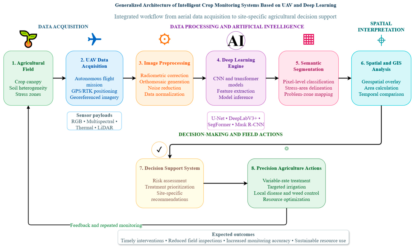
A review of current research indicates that intelligent crop monitoring is gradually shifting from the use of individual image analysis algorithms to the development of comprehensive hardware–software systems in which artificial intelligence algorithms are integrated with decision-support tools and instruments for managing complex technical systems [25,26,27,28,29]. The typical architecture of such solutions encompasses sequential stages of geospatial data collection using UAVs, image preprocessing, the application of deep learning models, semantic segmentation of problem areas, spatial analysis of results, and the generation of recommendations for performing differentiated agrotechnological operations. A generalized architecture of modern intelligent crop monitoring systems is shown in Figure 1.

As shown in Figure 1, the intelligent monitoring process is cyclical. The results of spatial analysis and the decision support system are used to plan local agronomic measures, after which data is collected again. This feedback loop ensures regular updates on the condition of crops, evaluation of the effectiveness of implemented operations, and timely adjustments to management decisions. At the same time, a review of the literature shows that most existing studies implement only individual elements of this architecture, while fully automated end-to-end solutions remain under-researched.

1.3. Research Gap

Despite the rapid development of artificial intelligence, computer vision, and UAV technologies, many existing studies in precision agriculture remain focused on individual analytical tasks, including crop classification, weed detection, disease recognition, and semantic segmentation. Comparatively less attention has been paid to end-to-end workflows that connect UAV imagery, automated image analysis, spatial interpretation, and decision support within a single processing framework [18,20,32,33,34,35].

Systematic reviews from recent years show that modern computer vision methods achieve high accuracy rates when performing specific tasks; however, their use is largely limited to laboratory or experimental settings. At the same time, most models are evaluated using standard metrics such as Accuracy, Precision, Recall, F1-score, or Intersection over Union, while the issue of their practical integration into the production processes of agricultural enterprises has not been sufficiently studied [25,29]. Consequently, the outputs of automated image analysis are not always transformed into spatially explicit information that can be directly used to prioritize field inspection and support subsequent agronomic decision-making.

The limited generalizability of modern deep learning models remains a significant scientific challenge. Despite significant progress in the development of convolutional neural networks, transformer architectures, and semantic segmentation algorithms, their effectiveness depends largely on the characteristics of the training datasets. Changes in crop type, soil type, weather conditions, UAV flight altitude, sensor type, or agroclimatic zone often lead to a decrease in model accuracy, which significantly limits their potential for widespread practical application [29,32,34]. Furthermore, recent studies highlight the lack of open, representative datasets that would simultaneously cover different crops, growing seasons, sensor types, and natural and climatic conditions.

Another pressing issue is the integration of multimodal data. Most existing studies use only one type of information, obtained from RGB cameras, multispectral sensors, or thermal imaging sensors. At the same time, current trends in the development of digital agriculture are focused on the comprehensive use of diverse information sources, including data from UAVs, satellite remote sensing, ground-based IoT sensors, geographic information systems, and digital elevation models. However, effective methods for integrating such data, synchronizing it spatially and temporally, and analyzing it jointly using artificial intelligence remain underdeveloped [35,36,37].

The issue of transitioning from image analysis results to supporting managerial decision-making warrants special attention. An analysis of the current literature shows that most existing systems end at the classification or segmentation stage, while geospatial analysis, the automatic generation of maps of problem areas, the prioritization of agrotechnological measures, and the evaluation of management alternatives are implemented only in a few studies [35,36,37,38]. The lack of integrated mechanisms for interaction between artificial intelligence algorithms, geoinformation technologies, and decision support systems significantly limits the practical value of most of the proposed approaches.

In addition, modern deep learning models are characterized by high computational complexity and significant hardware requirements. This complicates their implementation directly on board unmanned aerial vehicles and limits the ability to analyze data in real time. Despite the active development of edge intelligence and edge AI concepts, most current research remains in the experimental testing phase, and questions regarding the optimization of models for autonomous operation on energy-efficient computing platforms remain unresolved [34,38,39].

An analysis of the current state of research leads to the conclusion that the main scientific gap lies not in the absence of specific computer vision algorithms or deep learning models, but in the insufficient integration of all components of intelligent monitoring within a single information and analytical system. There is a need to develop a comprehensive approach that would combine the automated collection of highly detailed geospatial data using UAVs, modern methods of deep learning and semantic segmentation, geoinformation analysis, multimodal data integration, and the generation of evidence-based recommendations to support managerial decision-making in precision agriculture technologies [37,38,39,40]. Similar approaches to integrating heterogeneous data and mathematically justifying the parameters of complex technical systems are also applied when modeling the energy systems of agricultural enterprises [24]. Risk-oriented planning approaches are also applied to agricultural production systems, particularly when assessing resource requirements and uncertainties associated with the procurement of agricultural raw materials [41,42,43].

1.4. Objective and Scientific Contribution

The objective of this study is to develop and computationally validate an intelligent crop-monitoring framework that integrates UAV RGB imagery, deep learning-based semantic segmentation, RGB-based spatial interpretation, vectorization of candidate RGB heterogeneity zones, and a decision-support module for prioritizing field inspection in precision agriculture.

Unlike approaches that consider image analysis and decision support as separate stages, the proposed framework integrates UAV image preprocessing, semantic segmentation, RGB-based spatial interpretation, vectorization of candidate problem zones, and monitoring prioritization within a unified information workflow. This enables the transformation of image-level model outputs into structured information for targeted field inspection.

The research concept involves the comprehensive use of modern Earth remote sensing technologies, unmanned aerial vehicles, computer vision algorithms, deep learning models, geographic information systems, and spatial analysis tools. The combination of these components enables the creation of a unified information cycle that ensures the automated collection, processing, analysis, and interpretation of data on the condition of agricultural crops, with the resulting findings subsequently used to support managerial decision-making. The concept of configuring spatially distributed decision-support systems is also used in modeling other geographically distributed security systems [5].

The scientific contribution of this study lies in the development of an integrated methodological framework that combines semantic segmentation of UAV RGB imagery with RGB-based proxy assessment, vectorization of candidate RGB heterogeneity zones, and multi-criteria prioritization of image regions for subsequent field monitoring.

The main contributions of this study are as follows:

• Development of an integrated crop-monitoring framework connecting UAV image processing, semantic segmentation, RGB-based spatial interpretation, and decision support within a unified workflow;
• Comparative evaluation of U-Net, DeepLabV3, and FCN architectures for binary semantic segmentation of agricultural vegetation in high-resolution UAV RGB images;
• Development of an RGB-based procedure for identifying and vectorizing candidate RGB heterogeneity zones from segmented vegetation regions and quantitatively characterizing their spatial properties;
• Development of a decision-support procedure that integrates RGB-based heterogeneity indicators and spatial characteristics to prioritize image regions for subsequent field inspection.

The practical value of the proposed approach lies in its potential to serve as a foundation for developing modern digital platforms for crop monitoring, designed to identify problem areas in a timely manner, optimize the use of material and technical resources, improve the efficiency of field operations, and support decision-making in precision agriculture systems.

2. Materials and Methods

2.1. General Concept and Research Methodology

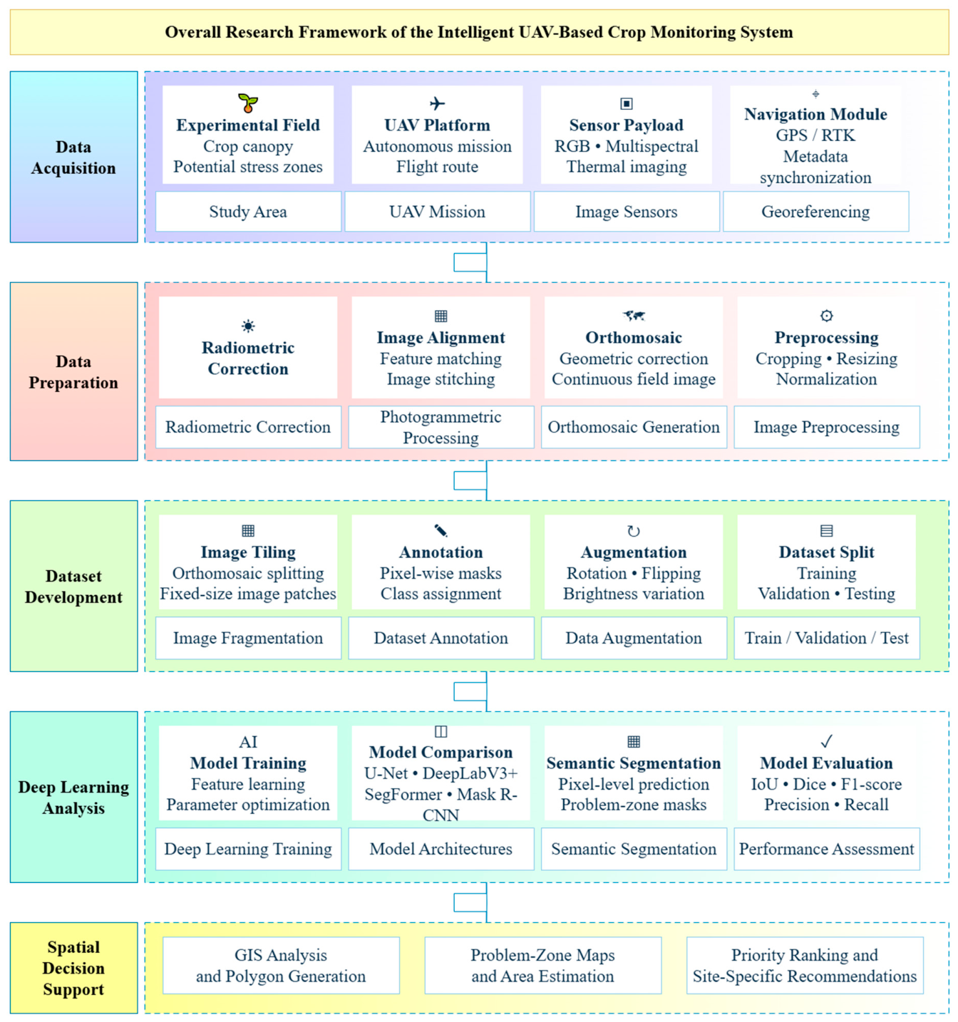
The research methodology is designed as a sequential process for transforming UAV crop imagery into structured information about vegetation cover and candidate problem zones. The experimental workflow combines dataset preparation, semantic segmentation, RGB-based spatial interpretation, vectorization, and decision-support analysis. A complementary UAV acquisition and geospatial processing architecture is proposed for subsequent field deployment. This approach is consistent with current trends in UAV monitoring, in which individual data collection and analysis operations are integrated into a single information process [2,17,18,21].

The primary model-development and internal evaluation experiments were performed using high-resolution RGB imagery and corresponding reference masks from the open-access dataset acquired using a DJI Air 2S UAV (SZ DJI Technology Co., Ltd., Shenzhen, China). In addition, RGB imagery independently acquired with a DJI Mavic 3 Multispectral (SZ DJI Technology Co., Ltd., Shenzhen, China) was used for pilot field acquisition and external validation of the selected U-Net-ResNet50 model. Multispectral and thermal channels were not used for model training or quantitative segmentation evaluation in the present study.

In the proposed field-deployment workflow, UAV imagery may be acquired using RGB or multispectral sensors together with positioning metadata required for subsequent geospatial processing. In the present study, this acquisition workflow was pilot-tested using the DJI Mavic 3 Multispectral, while the primary model-development experiments remained based on the open DJI Air 2S RGB dataset [9,17,18].

For future field deployment, the acquired UAV imagery can undergo radiometric and geometric correction, photogrammetric alignment, and orthomosaic generation. In the experimental part of this study, the RGB images and corresponding reference masks available in the open dataset were used directly and divided into equal 512 × 512-pixel patches for subsequent model development. The specific parameters of photogrammetric processing, the size of the fragments, and the normalization method are presented in Section 2.5.

Each source RGB image in the open dataset was accompanied by a corresponding pixel-wise reference mask. During tiling, identical spatial cropping was applied to both the RGB image and its reference mask, after which the resulting image–mask patches were assigned to the training, validation, and test subsets. This division takes into account the spatial origin of the images to ensure that adjacent fragments from the same area do not end up in both the training and test sets simultaneously. This reduces the risk of data leakage and ensures a more objective assessment of the model’s ability to handle new areas [23,25].

During the deep learning phase, the models are trained to perform pixel-level recognition of classes defined in the annotation protocol. The models produce pixel-level segmentation masks that reflect the spatial distribution of annotated vegetation patches and serve as the basis for further spatial analysis and assessment of potential problem areas. The models are compared using identical sample structures and consistent training conditions. IoU, the Dice coefficient, Precision, Recall, and the F1-score are used for evaluation, which allows for separate consideration of localization accuracy and errors related to missed or incorrectly detected pixels [6,22,23].

In the final experimental stage, the segmentation results are combined with RGB-based vegetation indicators to identify candidate RGB heterogeneity zones. These zones are converted into image-space vector objects for which pixel-based coordinates, geometric boundaries, and relative areas are calculated. The resulting indicators are subsequently used by the decision-support module to prioritize image regions for further field inspection. In future georeferenced field deployment, these vector objects can be transformed into geographic coordinates and integrated with GIS platforms.

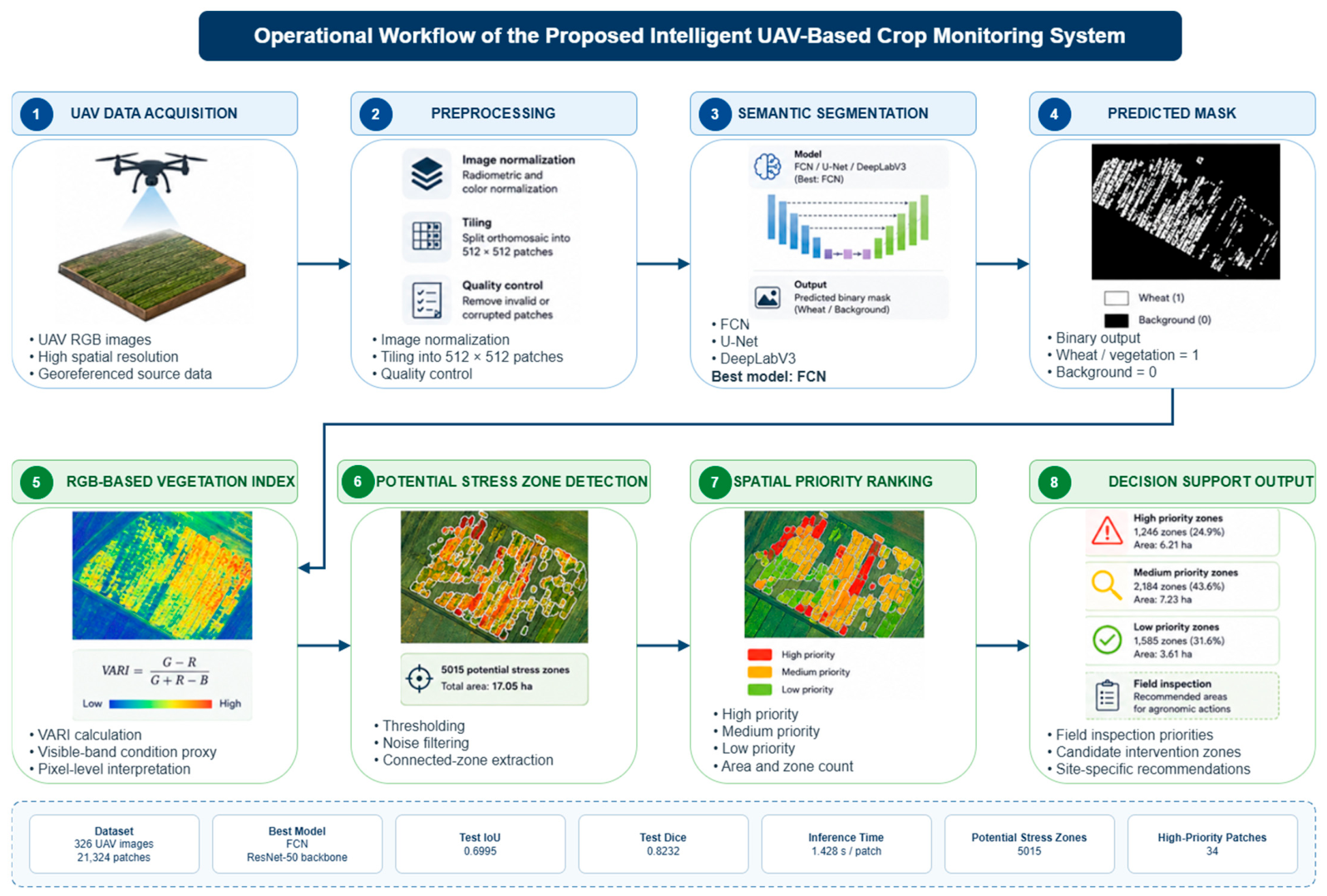
Thus, Figure 2 illustrates the overall framework of the proposed intelligent crop-monitoring system. The following sections describe the experimental dataset, proposed UAV hardware configuration and flight protocol, preprocessing procedures, dataset preparation, deep learning models, training strategy, spatial interpretation, and decision-support procedures.

2.2. Experimental UAV Data Set

To experimentally validate the proposed intelligent monitoring system, we used the open dataset “High-Resolution RGB Images and Corresponding Masks of Agricultural Fields,” available in the open repository Zenodo (Record 12607112) [42]. The use of an open dataset ensures the reproducibility of experiments, the possibility of independent verification of the obtained results, and a fair comparison of the performance of different deep learning models under identical conditions.

The dataset contains high-resolution RGB aerial images of agricultural fields captured using a DJI Air 2S unmanned aerial vehicle, together with corresponding reference masks. According to the repository description, the imagery covers several agricultural categories, including orchards, olive groves, green wheat, and vineyards. Because verified image-level crop labels were not available, no crop-specific subset was selected, and the dataset was treated as a mixed agricultural vegetation dataset. Following an automated data-integrity and image–mask pairing audit, 326 unambiguous valid RGB image–reference mask pairs were retained and used in the subsequent stages of the study.

The Zenodo repository description reports 325 source images; however, the reproducibility audit of the downloaded archive identified 326 unambiguous decodable RGB–mask pairs. Therefore, the retained count reported here reflects the actual set of image–mask pairs used in the final computational experiment.

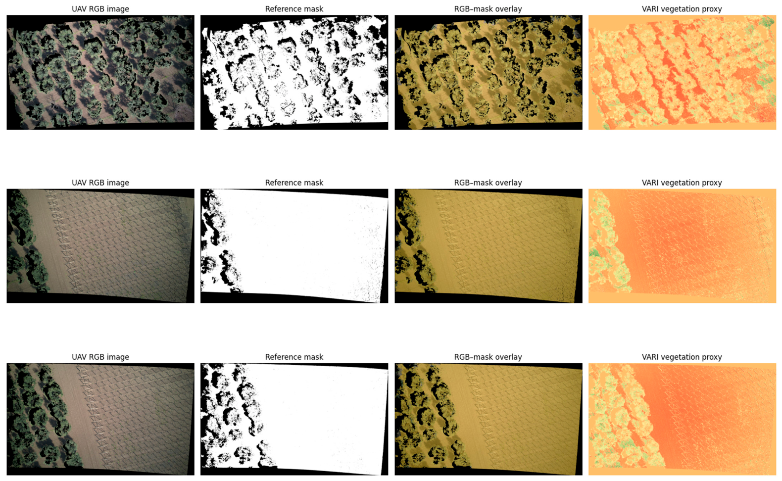
Examples of raw aerial images, reference masks, and their combinations are shown in Figure 3. These examples demonstrate varying spatial distributions of vegetation cover, heterogeneity in crop density, and the complexity of boundaries between vegetation and background objects. It is precisely these characteristics that make the dataset suitable for evaluating the effectiveness of modern semantic segmentation methods.

The main characteristics of the dataset used are presented in

Table 1. Composition and scope of the experimental UAV RGB dataset.

Characteristic	Value
Dataset source	Zenodo Record 12607112
UAV platform	DJI Air 2S
Dataset-level agricultural categories	Orchards; olive groves; green wheat; vineyards
Repository-reported RGB images	325
Retained decodable RGB–mask pairs in the reproducibility audit	326
Verified image-level crop labels	Not available
Segmentation target	Annotated agricultural vegetation vs. background/non-target
Generated patches	21,324
Patch size	512 × 512 pixels

. All source materials are provided in TIFF format, which allows the original quality of the aerial images to be preserved without loss, and the availability of pixel-level reference masks enables the use of supervised learning models for semantic segmentation.

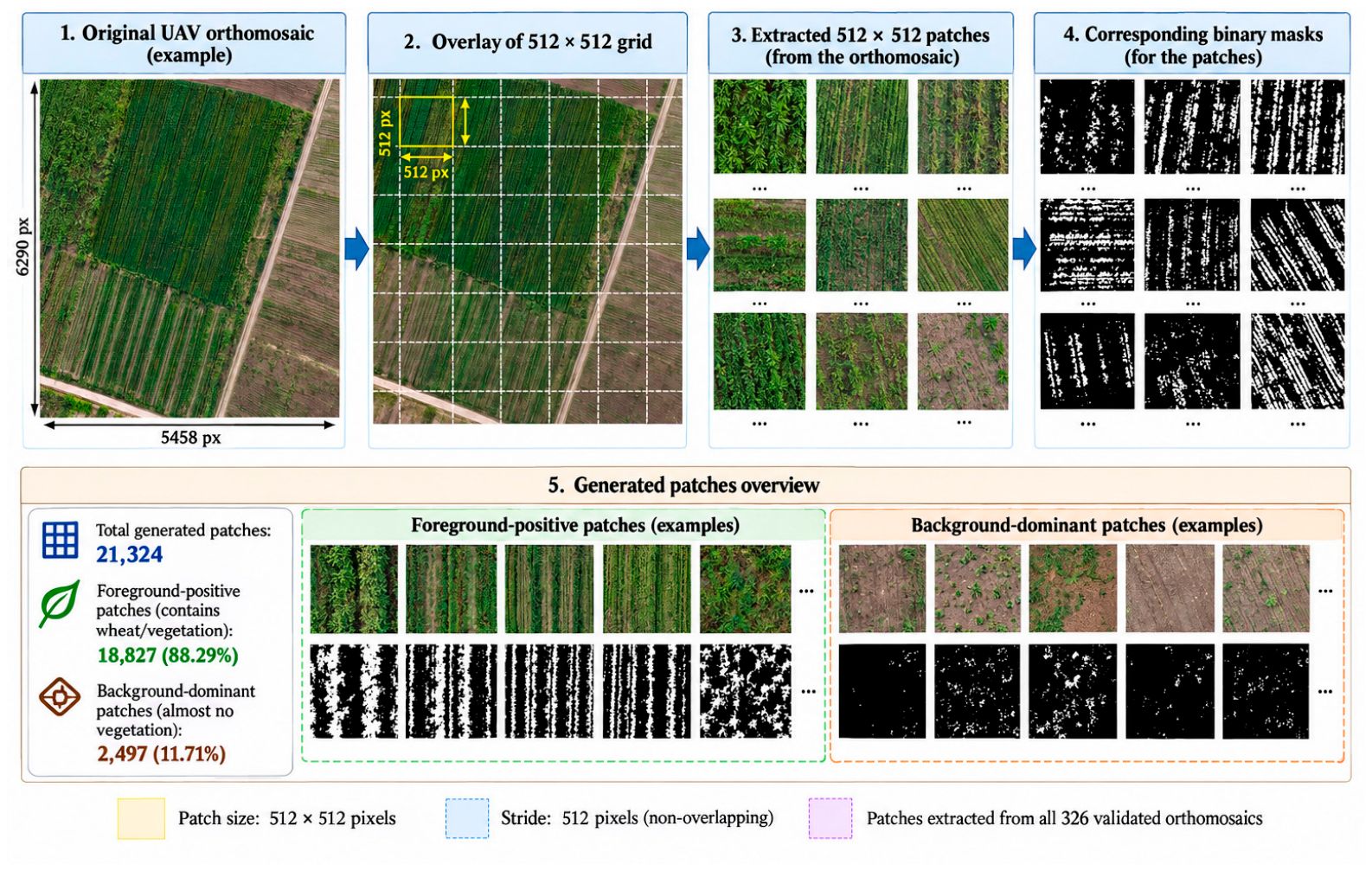
Analysis of the audited dataset showed that the source UAV RGB images have high spatial resolution and represent heterogeneous agricultural vegetation scenes. To standardize the model input, the 326 retained RGB image–mask pairs were automatically divided into 21,324 non-overlapping patches of 512 × 512 pixels. Based on the foreground fraction in the corresponding reference masks, 19,999 patches were classified as foreground-dominant (>50% vegetation pixels), whereas 1325 patches were classified as background-dominant (≤50% vegetation pixels).

Thus, the resulting patch dataset contains a broad range of vegetation-cover conditions and was used for subsequent model development, repeated grouped evaluation, and comparative semantic segmentation analysis (Table 1).

The source RGB data are individual high-resolution UAV images provided as raw drone outputs rather than orthomosaics. According to the repository documentation, the corresponding masks were generated using orthomosaic processing software and were not reported as manually delineated expert annotations. Therefore, throughout this study, they are referred to as reference masks rather than definitive ground-truth masks. The automated masks may contain residual uncertainties related to vegetation-boundary delineation, omission or commission errors, and local image–mask correspondence. The reproducibility audit verified file integrity, decodability, image–mask pairing, and dimensional consistency but did not constitute an independent expert re-annotation of the masks.

When creating the experimental dataset, special attention was paid to avoiding spatial information leakage between samples. To achieve this, the division into training, validation, and test sets was not performed randomly for individual fragments but was based on the original aerial photographs. This approach ensures that adjacent sections of the same field do not end up in different samples simultaneously, thereby ensuring a more objective assessment of the generalization ability of deep learning models.

2.3. DJI Mavic 3 Multispectral Platform and Pilot Field Validation

The DJI Mavic 3 Multispectral (Mavic 3M) was used for pilot field validation of the hardware component of the proposed crop-monitoring framework and to assess the feasibility of transferring the developed computational workflow to real UAV data acquisition conditions. The platform integrates an RGB camera, multispectral sensors, and RTK positioning capabilities, enabling the acquisition of spatially referenced field imagery.

The study comprised two complementary experimental components. The open-access RGB dataset acquired using a DJI Air 2S UAV was used for model training, internal validation, architecture selection, and repeated held-out testing. Separately, the DJI Mavic 3 Multispectral platform was used for pilot field data acquisition and independent external validation of the selected U-Net-ResNet50 model. The Mavic 3M imagery was not used for model training, hyperparameter selection, or internal model comparison. Instead, independently annotated RGB image patches acquired over a wheat field were used exclusively to evaluate the transferability of the trained model to a different UAV platform and real field conditions without additional retraining or fine-tuning.

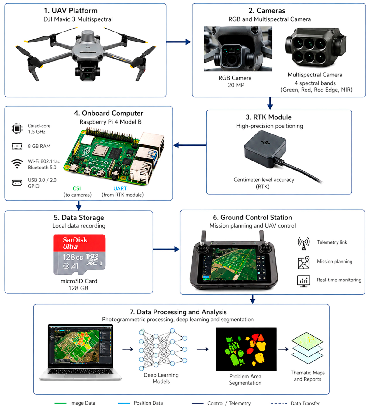
The architecture of the proposed hardware-software system is shown in Figure 4. It includes a UAV platform, RGB and multispectral cameras, an RTK module, a Raspberry Pi 4 single-board computer, a local data storage system, a ground control station, and a module for subsequent photogrammetric and intelligent data processing.

In the proposed hardware architecture, high-precision spatial georeferencing can be provided by the integrated RTK positioning system. The use of RTK correction data enables centimeter-level positioning and spatial synchronization of the acquired images with geographic coordinates. Such georeferencing is required for the subsequent generation of spatially referenced products and the integration of semantic segmentation results with geographic information systems.

The proposed architecture includes a Raspberry Pi 4 Model B single-board computer with 8 GB of RAM (Raspberry Pi Ltd., Cambridge, UK) as an auxiliary onboard computing unit. It can be used for telemetry recording, preliminary data processing, temporary data storage, and communication with external sensor modules. The specific implementation of interfaces between the onboard computer, UAV sensors, and positioning system depends on the selected hardware configuration and will be investigated during future field deployment of the system.

A 128 GB microSD memory card is proposed for local storage of telemetry and auxiliary monitoring data. The Raspberry Pi 4 supports USB 3.0, USB 2.0, Wi-Fi IEEE 802.11ac, Bluetooth 5.0, and GPIO interfaces, which provide flexibility for communication with peripheral devices and external sensor modules within the proposed monitoring architecture.

Flight mission planning and automated UAV control are to be carried out using DJI Pilot 2 (version v2.5.1.15, SZ DJI Technology Co., Ltd., Shenzhen, China) software, which allows users to create flight routes, set aerial photography parameters, monitor mission execution, and automatically synchronize telemetry data with photographic data. The general technical specifications of the hardware and software configuration proposed for future field deployment are presented in

Table 2. Technical specifications of the UAV platform and onboard hardware.

Component	Specification
UAV platform	DJI Mavic 3 Multispectral
UAV type	Multirotor
RGB camera	20 MP
RGB sensor	CMOS
Sensor resolution	20 MP
Multispectral channels	Green (560 nm), Red (650 nm), Red Edge (730 nm), Near Infrared (860 nm)
RTK positioning	Integrated DJI RTK module
Positioning accuracy	Centimeter-level (RTK)
Onboard computer	Raspberry Pi 4 Model B
Processor	Broadcom BCM2711
RAM	8 GB
Local storage	microSD 128 GB
Camera interface	CSI
RTK interface	UART
Wireless communication	Wi-Fi IEEE 802.11ac, Bluetooth 5.0
External interfaces	USB 3.0, USB 2.0, GPIO
Flight mission software	DJI Pilot 2
Coordinate synchronization	Automatic geotagging using GPS/RTK metadata

.

2.4. UAV Image Acquisition and Data Preparation

2.4.1. Flight Mission Planning

For pilot field validation of the proposed monitoring framework, UAV image acquisition was performed using the DJI Mavic 3 Multispectral platform. The field experiment was designed to verify UAV-based image acquisition, spatial referencing, and subsequent transfer of the acquired imagery to the developed processing workflow. Flight mission planning was performed in DJI Pilot 2, where the field boundaries, automatic flight route, altitude, UAV speed, and image-acquisition parameters were defined. A lawnmower-pattern flight route with 80% forward overlap and 70% side overlap was used to support orthomosaic generation.

The pilot flight was conducted at an altitude of 100 m above ground level and a flight speed of 6 m·s⁻¹. The camera was oriented in the nadir direction (90°), with 80% forward overlap and 70% side overlap. Image acquisition was performed between 10:00 and 13:00 under clear to partly cloudy conditions, with wind speed not exceeding 3.2 m·s⁻¹. The main parameters of the pilot field experiment are summarized in

Table 3. Parameters of the pilot UAV field-acquisition experiment using the DJI Mavic 3 Multispectral.

Parameter	Value
UAV platform	DJI Mavic 3 Multispectral
Flight altitude	100 m
Flight speed	6 m·s−1
Camera angle	90° (Nadir)
Forward overlap	80%
Side overlap	70%
Flight time	10:00–13:00
Weather conditions	Clear to partly cloudy
Wind speed	≤3.2 m·s−1
RGB image format	JPEG
Multispectral format	TIFF
Positioning	RTK
Estimated RGB GSD at 100 m	2.69 cm·pixel−1
Estimated multispectral GSD at 100 m	4.61 cm·pixel−1

.

The spatial resolution of the images (Ground Sampling Distance, GSD) was determined using the classical photogrammetric equation:

$$\mathit{GSD}={\displaystyle \frac{H\cdot p}{f}},$$

(1)

where H—flight altitude above the field surface, m; p—physical size of the sensor pixel, mm; f—focal length of the lens, mm.

For the proposed flight altitude of 100 m, the estimated GSD is approximately 2.69 cm·pixel⁻¹ for the RGB camera and 4.61 cm·pixel⁻¹ for the multispectral camera. These values characterize the proposed Mavic 3M field-acquisition configuration and were not used to determine the spatial resolution of the open RGB dataset employed for experimental validation. The main parameters of the proposed flight protocol are presented in Table 3.

2.4.2. Image Preprocessing

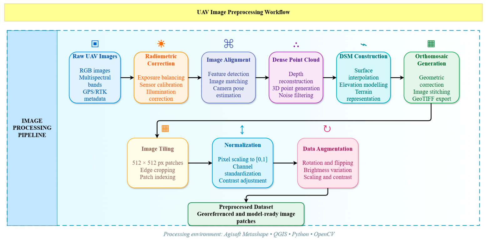
Preprocessing of aerial photographs in the proposed system involves the use of Agisoft Metashape Professional 2.1.2 (Agisoft LLC, St. Petersburg, Russia) for photogrammetric processing, QGIS 3.34 LTR for geospatial analysis, and Python 3.10.12 with OpenCV 4.10.0 for automated image preparation for training deep learning models. When using georeferenced data, the results can be transformed into a unified coordinate system–WGS 84/UTM Zone 35N (EPSG:32635)–which enables their subsequent integration with geographic information systems.

The proposed preprocessing pipeline includes radiometric correction, automatic image alignment, the generation of a dense point cloud and a digital surface model (DSM), and the creation of an orthomosaic. Upon completion of photogrammetric processing, the orthophoto is exported in GeoTIFF format and automatically divided into 512 × 512-pixel segments, which are used for further training of semantic segmentation models.

For the experimental validation performed using the open Zenodo RGB dataset, the available RGB images and corresponding reference masks were used directly. The experimental preprocessing included image–mask integrity verification, image tiling into 512 × 512-pixel patches, normalization, and preparation of the data for semantic segmentation. No additional UAV image acquisition or RTK-based photogrammetric reconstruction was performed as part of the experimental validation reported in this study. The overall preprocessing sequence is shown in Figure 5.

The proposed preprocessing pipeline generates a standardized set of image segments suitable for subsequent annotation and training of semantic segmentation models. The combination of photogrammetric processing, normalization, and augmentation reduces the impact of variations in lighting, scale, and image orientation, thereby improving the robustness of the models when analyzing new aerial images. For the experimental validation, only those preprocessing operations applicable to the available open dataset were performed, namely image–mask integrity verification, tiling, resizing, normalization, and data preparation for semantic segmentation. Radiometric correction, RTK-based georeferencing, photogrammetric reconstruction, DSM generation, and orthomosaic generation belong to the proposed field-deployment workflow and were not performed in the current experiment.

2.5. Deep Learning Dataset and Model Development

2.5.1. Dataset Preparation

After preprocessing, the original RGB images were automatically divided into non-overlapping patches measuring 512 × 512 pixels, which were used as the basic units for training semantic segmentation models. This approach preserved sufficient spatial context for vegetation-cover analysis while enabling efficient use of computational resources during model training.

Experimental validation was performed using the open-access dataset “High-Resolution RGB Images and Corresponding Masks of Agricultural Fields”, which contains high-resolution individual UAV RGB images and corresponding software-generated reference masks [42]. Because verified image-level crop labels were unavailable, the dataset was treated as a mixed agricultural vegetation dataset rather than a winter-wheat-specific subset. The 326 retained image–mask pairs yielded 21,324 non-overlapping patches, including 19,999 foreground-dominant and 1325 background-dominant patches.

For the open Zenodo dataset, the supplied reference masks were used directly for model development and internal evaluation; no additional manual pixel-wise re-annotation of the Zenodo masks was performed. The independent Mavic 3M field-validation subset was annotated separately to obtain vegetation reference masks for external model evaluation. The models were trained using a two-class semantic segmentation scheme comprising the following classes:

(1)

Background/non-target—background and non-target objects;

(2)

Annotated vegetation region—pixels belonging to the vegetation regions represented by the reference masks.

The total number of generated segments was defined as:

N = N_train + N_val + N_test,

(2)

where N_train, N_val and N_test are the number of fragments in the training, validation, and test sets, respectively.

To reduce source-image-level information leakage, a source-image-grouped holdout strategy was used. All patches originating from the same source UAV image were assigned exclusively to the training, validation, or test subset within each repeat. This grouping prevents patches from the same source image from appearing in different subsets; however, it does not guarantee full geospatial independence because spatial overlap between different source UAV images could not be excluded. Verified field identifiers and geospatial metadata sufficient to reconstruct non-overlapping field-level blocks were not available for the open dataset. Therefore, the adopted procedure is referred to throughout the manuscript as source-image-grouped splitting rather than spatially independent splitting (

Table 4. Structure of the experimental UAV image dataset.

Seed	Training Source Images	Training Patches	Validation Source Images	Validation Patches	Test Source Images	Test Patches
42	228	14,872	49	3203	49	3249
123	228	14,910	49	3127	49	3287
2026	228	14,950	49	3251	49	3123

).

In each repeated experiment, all 21,324 retained patches were used, with no patch-level subsampling. The grouping procedure ensured that patches derived from the same source image were assigned exclusively to one subset within a given repeat.

2.5.2. Deep Learning Models

Three deep learning architectures were evaluated for semantic segmentation: U-Net-ResNet50, DeepLabV3-ResNet50, and FCN-ResNet50. These models were selected due to their different architectural designs and widespread use in the analysis of high-resolution aerial images.

The FCN architecture implements a fully convolutional approach to pixel-wise image classification without using fully connected layers. U-Net uses an encoder–decoder structure with skip connections, which combine high-level semantic features with detailed spatial information. DeepLabV3 employs atrous convolutions and multiscale context aggregation to capture vegetation patterns at multiple spatial scales.

The source RGB images were divided into 512 × 512-pixel patches and resized to 256 × 256 pixels for model training. To ensure a fair architectural comparison, all three evaluated models used a ResNet-50 encoder/backbone initialized with ImageNet1K V2 pretrained weights. U-Net was implemented as a ResNet50-based encoder–decoder architecture with skip connections, while DeepLabV3-ResNet50 and FCN-ResNet50 used their standard architecture-specific segmentation heads. Thus, the compared models differed primarily in their decoder/head design rather than in backbone initialization or transfer-learning strategy.

The models were trained using a composite loss function combining weighted cross-entropy and Dice loss:

L = λL_CE + (1 − λ)L_Dice,

(3)

where L_CE—categorical cross-entropy, and L_Dice—Dice loss.

λ_CE = λ_Dice = 0.5.

(4)

Equal weighting was used to balance pixel-wise classification accuracy and spatial overlap during model optimization.

The cross-entropy loss function was defined using the formula:

$$L_{\mathit{CE}}=-{\displaystyle \frac{1}{N}}{\displaystyle \sum _{i=1}^N{\displaystyle \sum _{c=1}^C{y}_{\mathit{ic}}\log (p_{\mathit{ic}}+\epsilon )}}.$$

(5)

where N is the number of pixels; C is the number of semantic classes, with C = 2; y_ic is the reference-label indicator for pixel i and class c; p_ic is the corresponding probability predicted by the model after the softmax transformation; and ε is a small constant introduced for numerical stability.

The Dice Loss function was calculated using the following expression:

$$L_{\mathit{Dice}}=1-{\displaystyle \frac{1}{C}}{\displaystyle \sum _{c=1}^C\frac{2{\displaystyle \sum _{i=1}^N{p}_{\mathit{ic}}}{y}_{\mathit{ic}}+\epsilon }{{\displaystyle {\displaystyle \sum _{i=1}^N}{p}_{\mathit{ic}}}+{\displaystyle {\displaystyle \sum _{i=1}^N}{y}_{\mathit{ic}}}+\epsilon }}.$$

(6)

where N is the number of pixels; C is the number of classes; p_ic is the predicted probability for pixel i and class c; y_ic is the corresponding one-hot encoded reference-label value; and ε = 10⁻⁶ is used to ensure numerical stability.

The main configurations of the evaluated models are summarized in

Table 5. Configuration of the evaluated deep learning models under the standardized comparison protocol.

Model	Encoder/Backbone	Input Size	Backbone Initialization	Decoder/Head Initialization	Parameters	Loss Function
U-Net-ResNet50	ResNet-50	256 × 256	ImageNet1K V2	Random	32.51 M	Cross-Entropy + Dice
DeepLabV3-ResNet50	ResNet-50	256 × 256	ImageNet1K V2	Random	39.63 M	Cross-Entropy + Dice
FCN-ResNet50	ResNet-50	256 × 256	ImageNet1K V2	Random	32.95 M	Cross-Entropy + Dice

. All architectures used the same 256 × 256 input resolution, ResNet-50 backbone, ImageNet1K V2 backbone initialization, combined Cross-Entropy and Dice loss, and common optimization protocol. Architecture-specific decoder/head components were randomly initialized. This standardization removes the transfer-learning asymmetry present in the previous experimental design and provides a more controlled basis for comparing the segmentation architectures (Table 5).

2.5.3. Training Strategy

All models were trained under identical experimental conditions using the PyTorch library. To ensure a fair comparison of architectures, we used the same input image size, a common loss function, the same optimization algorithm, and a unified evaluation strategy. All models were trained within the same experimental evaluation framework using the PyTorch library. The same input resolution, loss formulation, optimization algorithm, dataset-splitting strategy, and evaluation metrics were applied. For all three architectures, the ResNet-50 backbone was initialized using the same ImageNet1K V2 pretrained weights, whereas the architecture-specific decoder or segmentation head was randomly initialized.

Parameter optimization was performed using the AdamW algorithm, which combines adaptive learning rate adjustment with weight regularization. The best model was selected based on the maximum Intersection over Union (IoU) value obtained on the validation set:

$$e^{*}=\underset{e\in \{1,\dots ,E\}}{\mathrm{argmax}}{\mathit{IoU}}_{\mathrm{val}}^{(e)}.$$

(7)

where e^* denotes the epoch corresponding to the highest validation IoU; E is the total number of completed training epochs; and ${\mathit{IoU}}_{\mathrm{val}}^{(e)}$ is the validation IoU obtained after epoch e. The model weights corresponding to e^* were retained as the final checkpoint.

Early stopping was controlled by validation vegetation IoU. Training was required to continue for at least 10 epochs and was allowed to proceed for a maximum of 30 epochs. After the minimum epoch requirement was satisfied, training was terminated only when validation IoU failed to improve for five consecutive epochs. The checkpoint corresponding to the highest validation IoU was retained for evaluation. Thus, an early best epoch did not imply immediate termination of training. The main parameters of the training process are presented in

Table 6. Main training parameters of the evaluated deep learning models.

Parameter	Value
Model input size	256 × 256 pixels
Source patch size	512 × 512 pixels
Backbone	ResNet-50 for all architectures
Backbone initialization	ImageNet1K V2 pretrained
Decoder/head initialization	Random
Optimizer	AdamW
Loss function	Cross-Entropy + Dice
Model selection criterion	Highest mean validation vegetation IoU across repeated runs
Repeated seeds	42, 123, 2026

.

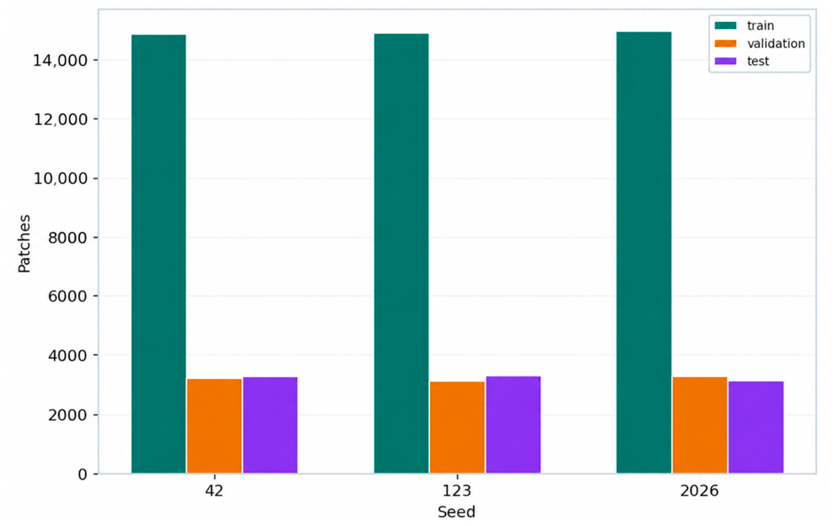
The comparative evaluation was performed in full-data mode without patch subsampling. To assess the robustness of the results, three repeated source-image-grouped holdout experiments were conducted using random seeds 42, 123, and 2026. Each repeat used all 21,324 retained image patches. For seed 42, the training, validation, and held-out test subsets contained 14,872, 3203, and 3249 patches, respectively; for seed 123, they contained 14,910, 3127, and 3287 patches; and for seed 2026, they contained 14,950, 3251, and 3123 patches. All patches originating from the same source image were assigned to a single subset within each repeat, and no source-image group overlap occurred between the training, validation, and test subsets. Model selection was based on the highest mean validation vegetation IoU across the three repeated experiments, whereas the test subsets remained held out until final evaluation. Performance was summarized using the mean and standard deviation across the three repeats, and uncertainty was additionally assessed using 1000-replicate group-bootstrap 95% confidence intervals.

Data augmentation was applied only to the training subset and was performed synchronously for each RGB image and its corresponding reference mask. Horizontal and vertical flips were independently applied with probabilities of 0.5. Random rotations were selected uniformly from 0°, 90°, 180°, and 270°. In addition, an RGB-only brightness/contrast-like perturbation was applied with a probability of 0.4 using a multiplicative factor uniformly sampled from 0.85 to 1.15 and an additive intensity shift from −10 to +10. Validation and test images were not augmented. After resizing to 256 × 256 pixels, RGB values were normalized using the ImageNet mean and standard deviation.

The use of a unified training strategy and identical optimization parameters ensured a fair comparison of the architectures under study and allowed for an objective assessment of their ability to perform semantic segmentation of high-resolution UAV images.

External field validation was additionally performed using RGB imagery acquired with the DJI Mavic 3 Multispectral over a wheat field during the pilot experiment described in Section 2.4. A representative set of non-overlapping 512 × 512-pixel image patches was selected from the field imagery and manually annotated to obtain independent vegetation reference masks. The selected U-Net-ResNet50 model, trained exclusively on the open DJI Air 2S dataset, was applied to the Mavic 3M image patches without additional fine-tuning or parameter adjustment. Segmentation performance was evaluated using Precision, Recall, vegetation IoU, and Dice coefficient calculated from globally aggregated pixel-level confusion counts. This procedure was used to assess the transferability of the trained model to independently acquired UAV imagery collected using a different platform and under real field conditions.

2.6. RGB-Based Spatial Interpretation and Decision-Support Algorithm

Following semantic segmentation, an RGB-based spatial analysis procedure was applied to the vegetation regions identified by the best-performing semantic segmentation model. The purpose of this stage was not to diagnose physiological crop stress, but to detect spatial heterogeneity in vegetation appearance and identify areas requiring subsequent field verification. Therefore, the detected regions are consistently referred to as candidate RGB heterogeneity zones. Such zones may reflect canopy gaps, soil exposure, shadows, senescence, crop-density differences, or other variations in RGB appearance and should not be interpreted as evidence of a specific physiological disorder.

For each analyzed image patch, the red (R), green (G), and blue (B) channels were converted from the original 8-bit representation to floating-point values in the range [0,1]. Three visible-band vegetation indices were then calculated: the Visible Atmospherically Resistant Index (VARI), Excess Green Index (ExG), and Green Leaf Index (GLI).

The VARI index was calculated as:

$${\mathit{VARI}}_i={\displaystyle \frac{G_i-R_i}{G_i+R_i-B_i+\epsilon }}.$$

(8)

where R_i, G_i and B_i are the normalized red, green, and blue channel values of pixel i, respectively; ε = 10⁻⁶ is a small constant introduced to prevent division by zero.

The Excess Green Index was calculated as:

$$E{x}_{G_i}=2G_i-R_i-B_i.$$

(9)

where $E{x}_{G_i}$ represents the relative predominance of the green component for pixel i.

The Green Leaf Index was determined as:

$${\mathit{GLI}}_i={\displaystyle \frac{2G_i-R_i-B_i}{2G_i+R_i+B_i+\epsilon }}.$$

(10)

The calculated VARI, ExG, and GLI values were restricted to the interval [−1,1]. To avoid forcing each image patch into the same relative index range, patch-specific normalization was not used in the final analysis. Instead, fixed normalization bounds were estimated exclusively from vegetation pixels in the training subset of the reference split. For each RGB vegetation index, the 5th and 95th percentiles of the training data were calculated once and subsequently applied unchanged to all held-out image patches:

$$I_k^{\mathit{norm}}=\mathrm{clip}\left({\displaystyle \frac{I_k-Q_{5,k}^{\mathit{train}}}{Q_{95,k}^{\mathit{train}}-Q_{5,k}^{\mathit{train}}+\epsilon }},0,1\right).$$

(11)

where I_k denotes the value of VARI, ExG, or GLI for pixel p; $Q_{5,k}^{\mathit{train}}$ and $Q_{95,k}^{\mathit{train}}$ are the 5th and 95th percentiles of index k, estimated exclusively from reference vegetation pixels in the training subset; and the clipping operation restricts the normalized value to [0,1].

The same normalization bounds were applied to every validation and held-out test patch. These percentiles serve only as fixed RGB scaling constants and should not be interpreted as physiologically validated thresholds.

The normalized vegetation indices were integrated into a single RGB Appearance Score. The relative contributions of VARI, ExG, and GLI were set to 0.40, 0.35, and 0.25, respectively:

$$C_i=0.40{\mathit{VARI}}_i^{*}+0.35\mathit{Ex}{G}_i^{*}+0.25{\mathit{GLI}}_i^{*}.$$

(12)

where ${\mathit{VARI}}_i^{*}$, $\mathit{Ex}{G}_i^{*}$ and ${\mathit{GLI}}_i^{*}$ are the robustly normalized values of the corresponding RGB vegetation indices.

Candidate RGB heterogeneity pixels were identified only within the vegetation mask predicted by the semantic segmentation model. A pixel was assigned to the candidate RGB heterogeneity class when its RGB Appearance Score was below 0.30:

$$M_i=\left\{\begin{array}{ll}1,\hfill & i\in M_{\mathrm{crop}}\mathrm{and}{C}_i<0.30,\hfill \\ 0,\hfill & \mathrm{otherwise},\hfill \end{array}\right..$$

(13)

where M_i is the binary candidate RGB heterogeneity mask; M_crop denotes the predicted vegetation mask.

The threshold of 0.30 was heuristically specified for the proof-of-concept RGB screening procedure and should not be interpreted as a physiologically validated threshold for a specific type of crop stress.

To suppress isolated noise, the initial candidate RGB heterogeneity mask was processed using an 8-connected component analysis. Connected components with an area smaller than 30 pixels were removed. The remaining connected components were considered individual RGB-based candidate RGB heterogeneity zones.

For each image patch j, the relative proportion of candidate RGB heterogeneity pixels within the predicted vegetation region was determined as:

$$S_j={\displaystyle \frac{N_{\mathrm{stress},j}}{N_{\mathrm{crop},j}}}.$$

(14)

where N_stress,j is the number of pixels retained in the candidate RGB heterogeneity mask, and N_crop,j is the total number of pixels classified as vegetation in image patch j.

For presentation as a percentage, S_j was multiplied by 100%.

The average RGB-based condition of the vegetation within each image patch was characterized by the Mean RGB Appearance Score:

$${\overline{C}}_j={\displaystyle \frac{1}{N_{\mathrm{crop},j}}}{\displaystyle \sum _{i\in M_{\mathrm{crop},j}}{C}_i}.$$

(15)

where ${\overline{C}}_j$ represents the Mean RGB Appearance Score for image patch j.

After filtering, each retained connected component was represented as an image-space vector object characterized by its pixel area, centroid, contour geometry, and bounding box. Patch-level coordinates were transformed to the coordinate system of the corresponding source image using the known patch offsets. The resulting coordinates are expressed exclusively in source-image pixels and are not geographic coordinates. No affine transformation to a projected coordinate reference system was applied to the Zenodo RGB dataset because the required georeferencing metadata were not available. Therefore, the resulting polygons should be interpreted as localized computer-vision vector objects rather than GIS features.

The derived RGB indicators were subsequently integrated into a decision-support procedure for prioritizing image patches requiring further field inspection. For each analyzed image patch j, an integrated Priority Score was calculated as:

$$P_j=0.50S_j+0.30(1-{\overline{C}}_j)+0.20{\displaystyle \frac{Z_j}{Z_{\max }}}.$$

(16)

where P_j ∈ [0,1] is the integrated monitoring priority score; S_j is the normalized share of candidate RGB heterogeneity pixels; ${\overline{C}}_j$ is the Mean RGB Appearance Score; Z_j is the number of candidate RGB heterogeneity zones detected in image patch j; and Z_max is the maximum number of candidate RGB heterogeneity zones observed among all analyzed image patches.

Thus, the Priority Score simultaneously accounts for the relative extent of RGB-based vegetation heterogeneity, the RGB Appearance Score deficit, and the spatial fragmentation of the detected candidate RGB heterogeneity zones.

Based on the calculated Priority Score, image patches were assigned to one of three monitoring-priority classes:

$${\mathit{Priority}}_j=\left\{\begin{array}{ll}\mathit{Low},\hfill & P_j<0.20,\hfill \\ \mathit{Medium},\hfill & 0.20\le P_j<0.45,\hfill \\ \mathit{High},\hfill & P_j\ge 0.45.\hfill \end{array}\right..$$

(17)

Low-priority patches were assigned to routine UAV monitoring, medium-priority patches were recommended for targeted field inspection and verification of crop condition, and high-priority patches were assigned the highest priority for ground verification and subsequent site-specific agronomic assessment.

The baseline parameters of the RGB-based decision-support procedure were defined as follows: VARI, ExG, and GLI weights of 0.40, 0.35, and 0.25, respectively; an RGB heterogeneity threshold of 0.30; Priority Score weights of 0.50, 0.30, and 0.20; and Low–Medium–High priority boundaries of 0.20 and 0.45. These parameters were treated as heuristic baseline settings rather than agronomically calibrated constants. Their robustness was therefore evaluated through a dedicated sensitivity and ablation analysis described below.

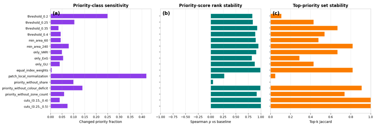
Sensitivity analysis was performed on a deterministic subset of 200 held-out image patches. One-at-a-time perturbations included RGB heterogeneity thresholds of 0.20, 0.25, 0.35, and 0.40; minimum connected-component areas of 60 and 240 source-image pixels; single-index VARI, ExG, and GLI formulations; equal RGB-index weights; removal of individual Priority Score components; alternative priority-class boundaries of 0.15/0.40 and 0.25/0.50; and patch-local normalization as an ablation comparator. In addition, 40 joint perturbation scenarios were generated by simultaneously varying the normalized RGB-index and Priority Score weights by ±20%, the heterogeneity threshold within 0.24–0.36, and the priority boundaries within 0.16–0.24 and 0.40–0.50.

Robustness was assessed using Spearman rank correlation of Priority Scores relative to the baseline, Jaccard similarity of the top-20 ranked patches, the fraction of patches changing priority class, the mean RGB heterogeneity share, the number of detected zones, and the number of high-priority patches. The analysis was used solely to assess robustness of the heuristic formulation and should not be interpreted as empirical agronomic calibration.

3. Results

3.1. Implementation of the Proposed Intelligent Crop Monitoring System

To verify the functionality of the proposed intelligent automated crop monitoring system, a complete software pipeline was implemented, covering all key stages of data processing–from the analysis of raw UAV images to the generation of recommendations regarding spatially localized areas requiring further inspection. The implementation was carried out in Python 3.10.12 using PyTorch 2.2.2, OpenCV 4.10.0, NumPy 1.26.4, Pandas 2.2.2, GeoPandas 0.14.4, and scikit-image 0.23.2, which ensured the automated execution of all analysis stages.

Quantitative validation was performed using the open-access UAV RGB dataset described in Section 2.2, following the data-preparation and evaluation protocol presented in Section 2.4 and Section 2.5.

A general overview of the proposed system’s operation is shown in Figure 6. The system begins by loading the input UAV RGB images and corresponding reference masks. After normalization and automatic segmentation, the image fragments are transferred to the deep learning module, where semantic segmentation of vegetation cover is performed. The resulting segmentation masks are used for further spatial analysis, calculation of the VARI RGB index, and identification of candidate RGB heterogeneity zones. In the final stage, the system generates a priority map of plots and recommendations for their field inspection.

The implemented software pipeline integrated semantic segmentation, RGB-based spatial interpretation, image-space vectorization of candidate RGB heterogeneity zones, and monitoring-priority assessment. Quantitative segmentation evaluation was based on the open dataset, while UAV field acquisition was assessed separately in the pilot Mavic 3M experiment.

Thus, the implemented system provides an end-to-end cycle of automated analysis of UAV imagery–from the acquisition of raw data to the generation of information necessary to support decision-making in precision agriculture systems. This integration of modules for preprocessing, semantic segmentation, spatial analysis, and the assessment of candidate RGB heterogeneity zones lays the foundation for near-real-time monitoring after further computational optimization of crop conditions and the further development of intelligent agricultural management systems.

3.2. Characteristics of the Experimental UAV Dataset

An experimental validation of the proposed intelligent system was performed on the open dataset «High-Resolution RGB Images and Corresponding Masks of Agricultural Fields,» which contains individual high-resolution UAV RGB images of agricultural fields and corresponding software-generated semantic-segmentation reference masks. The RGB images represent raw UAV camera outputs rather than photogrammetrically generated orthomosaics. The experimental dataset comprised RGB images and corresponding reference masks from the mixed agricultural scenes provided in the Zenodo repository. These scenes include orchards, olive groves, green wheat, and vineyards. Because verified image-level crop metadata were unavailable, the analysis was not restricted to a single crop category. Therefore, all reported segmentation results refer to the broader task of agricultural vegetation segmentation.

In the first stage, an automated check of the dataset structure was performed, which included verifying the number of files, the consistency of image and mask dimensions, encoding modes, and spatial alignment. As shown in Figure 3, the check confirmed the presence of 326 valid pairs of RGB images and corresponding masks. All images contained three color channels (RGB), while the masks were represented as binary images with two class values. The spatial dimensions of the source UAV RGB images ranged approximately from 5092 × 2926 to 6287 × 3765 pixels, indicating significant variation in the areas of the study sites and the configurations of the flight routes.

Foreground coverage varied substantially among the source UAV images; the corresponding descriptive statistics are summarized in

Table 7. Statistical characteristics of the foreground coverage in the experimental UAV dataset.

Statistic	Foreground Share (%)
Mean	64.55
Median	81.24
Standard deviation	31.30
Minimum	4.56
25th percentile	66.42
75th percentile	85.60
Maximum	89.96

. The 326 retained RGB image–mask pairs yielded 21,324 non-overlapping patches of 512 × 512 pixels, comprising 19,999 foreground-dominant and 1325 background-dominant patches (Figure 7).

Repeated source-image-grouped holdout experiments produced comparable training, validation, and held-out test subset sizes and foreground proportions across seeds 42, 123, and 2026 (Figure 8).

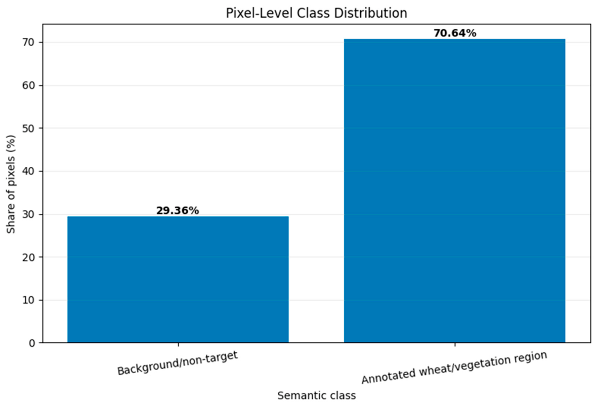
The class distribution at the individual-pixel level was analyzed separately. The results are shown in Figure 9. It was found that 3,948,918,946 pixels (70.64%) belong to the «Annotated vegetation region» class, while 1,641,039,710 pixels (29.36%) belong to the «Background/non-target» class. This ratio indicates a moderate class imbalance, which is typical for semantic segmentation tasks involving high-resolution UAV images. At the same time, the predominance of the target class ensures a sufficient number of training examples for the stable optimization of deep learning model parameters.

An in-depth analysis of the compiled dataset is presented in Table 7. The results indicate significant spatial heterogeneity in the experimental data. The average vegetation cover across individual source UAV images was 64.55%, while the median value reached 81.24%. This difference between the mean and the median is explained by the presence of individual areas with low vegetation density or a significant proportion of bare soil. The minimum proportion of the target class was only 4.56%, while the maximum reached 89.96%, confirming the substantial variability in imaging conditions and crop structure.

The standard deviation (31.30%) also indicates a wide range of vegetation coverage across individual source UAV images. At the same time, the interquartile range (66.42–85.60%) shows that most images are characterized by a fairly high proportion of vegetation cover. This heterogeneity is a significant advantage of the resulting dataset, as it allows for the evaluation of the robustness of deep learning models not only in typical field areas but also under complex conditions associated with varying crop densities, heterogeneity in vegetation structure, and changes in surface texture characteristics.

Overall, the dataset provided heterogeneous agricultural vegetation scenes and a consistent basis for the subsequent repeated source-image-grouped comparison of the segmentation architectures.

3.3. Pilot Field Acquisition and External Model Validation Using the DJI Mavic 3 Multispectral

A pilot field experiment was conducted using the DJI Mavic 3 Multispectral platform to verify the practical applicability of the proposed UAV data-acquisition workflow. The experiment confirmed the feasibility of acquiring high-resolution RGB imagery together with spatial positioning metadata under field conditions and transferring the collected data to the subsequent image-processing workflow.

The pilot field experiment was used both to verify the UAV data-acquisition workflow and to provide an independent external evaluation of the selected segmentation model. The Mavic 3M imagery was not used for model training, architecture selection, or internal validation. Instead, the selected U-Net-ResNet50 model was applied to independently annotated RGB image patches acquired over the wheat field without additional retraining or fine-tuning. This enabled a quantitative assessment of model transferability under independent field conditions and using a different UAV platform.

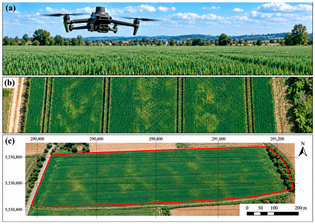
Figure 10 presents the results of the pilot field validation of the DJI Mavic 3 Multispectral platform in the vicinity of Dubliany, Lviv Oblast, Ukraine. Panel (a) illustrates the UAV used during the field survey of wheat crops, panel (b) shows a representative RGB image acquired during the flight, and panel (c) presents the spatially referenced orthomosaic of the study field with the field boundary and coordinate grid. These results demonstrate the feasibility of UAV-based image acquisition, spatial referencing, and transfer of the acquired data to the subsequent processing workflow under the tested pilot conditions.

The Mavic 3M imagery was not used for training, model selection, or internal validation. Instead, an independently annotated subset of the pilot field imagery was used exclusively for external evaluation of the selected U-Net-ResNet50 model. Thus, the field experiment provided an additional assessment of model transferability to imagery acquired with a different UAV platform and under independent field conditions.

To complement the hardware and acquisition validation, the selected U-Net-ResNet50 model was additionally evaluated on independently acquired Mavic 3M RGB imagery from the wheat field (Figure 10). The model was applied without retraining or fine-tuning. Performance was quantified against manually prepared vegetation reference masks using the same pixel-level metrics as in the main experiment. The comparison between the internal held-out evaluation and the independent field validation is presented in

Table 8. Comparison of U-Net-ResNet50 segmentation performance on the open UAV dataset and independent DJI Mavic 3 Multispectral field imagery.

Evaluation Dataset	UAV Platform	Agricultural Scene	Model Adaptation	Precision	Recall	Vegetation IoU	Dice
Open UAV dataset, held-out test sets	DJI Air 2S	Mixed agricultural vegetation	Internal repeated grouped evaluation	0.9946 ± 0.0008	0.9931 ± 0.0021	0.9877 ± 0.0020	0.9938 ± 0.0010
Independent pilot field imagery	DJI Mavic 3 Multispectral	Wheat field, Dubliany, Lviv Oblast	External validation, no retraining	0.9323 ± 0.0009	0.9221 ± 0.0045	0.9115 ± 0.006	0.9214 ± 0.007

.

The independent Mavic 3M field validation showed lower segmentation performance than the internal DJI Air 2S evaluation, with Precision = 0.9323 ± 0.0009, Recall = 0.9221 ± 0.0045, IoU = 0.9115 ± 0.0060, and Dice = 0.9214 ± 0.0070. The decrease is expected under external field conditions and reflects differences in UAV platform, sensor characteristics, illumination, and scene structure. Nevertheless, the model retained high segmentation accuracy without retraining, indicating good cross-platform transferability and supporting its potential use for real-field monitoring.

3.4. Performance Evaluation of Deep Learning Models

All performance results reported in this section were obtained from the revised full-data experiments. No FAST_MODE subsampling was used. Each repeated experiment used all 21,324 retained patches, with source-image grouping maintained between the training, validation, and held-out test subsets.

After generating the experimental dataset, a comparative evaluation of three modern semantic segmentation architectures was performed: U-Net, DeepLabV3, and FCN. All models were trained under identical conditions using the same training, validation, and test sets, which ensured the objectivity of the comparison and eliminated the influence of differences in data structure on the final results.

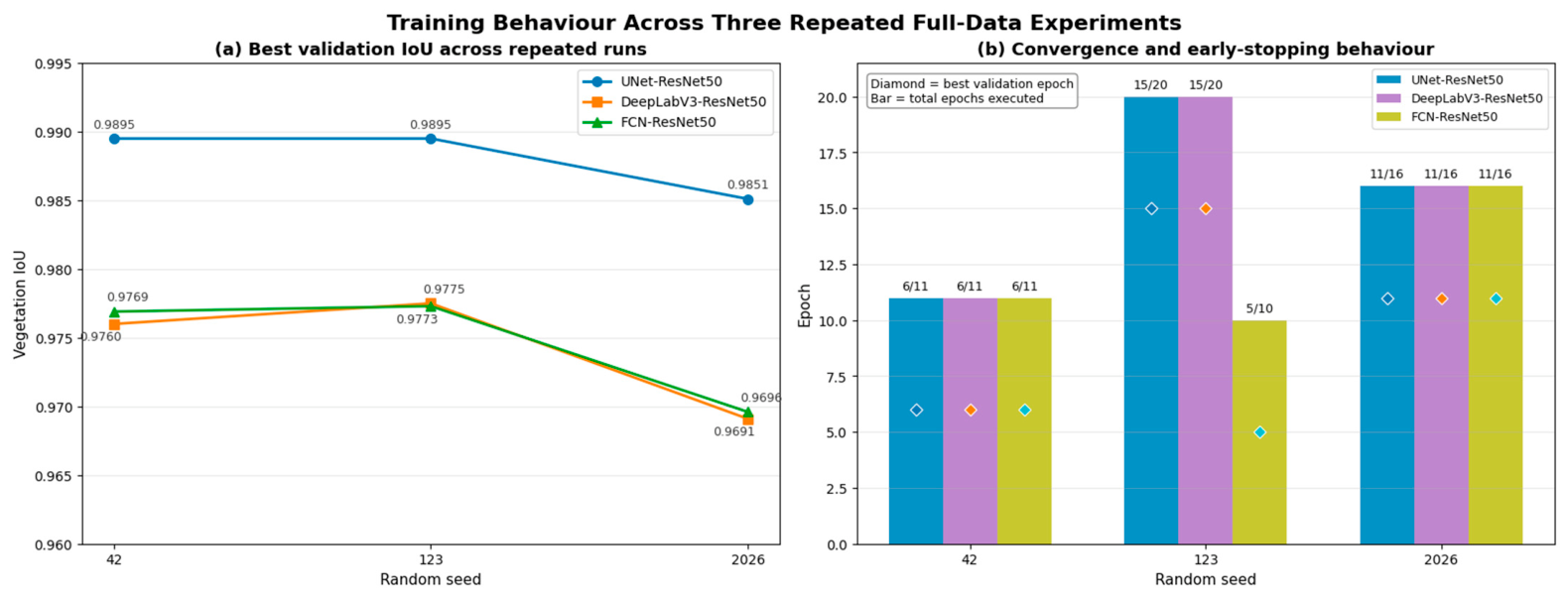
The full-data repeated evaluation substantially strengthened the statistical basis for comparing the three segmentation architectures. Each architecture was trained and evaluated in three source-image-grouped holdout experiments using random seeds 42, 123, and 2026, with all 21,324 retained image patches participating in each repeat (Figure 11).

U-Net-ResNet50 consistently achieved the highest validation IoU across all three repeated experiments. The best validation epochs varied among the models and data splits, while the convergence patterns indicate that all architectures reached stable solutions within 10–20 training epochs under the adopted early-stopping protocol.

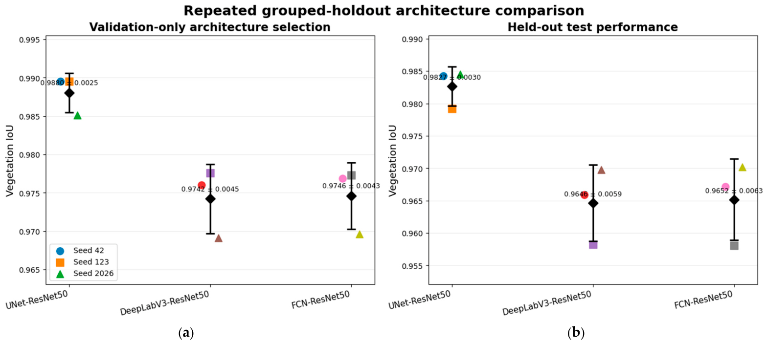
Architecture selection was performed exclusively on the validation subsets. U-Net-ResNet50 achieved the highest mean validation vegetation IoU of 0.9880 ± 0.0025, compared with 0.9746 ± 0.0043 for FCN-ResNet50 and 0.9742 ± 0.0045 for DeepLabV3-ResNet50. Therefore, U-Net-ResNet50 was selected for the subsequent spatial-analysis stage.

The same ranking was observed on the held-out test subsets, with U-Net-ResNet50 achieving the strongest mean segmentation performance and low variability across the three repeated source-image-grouped experiments (

Table 9. Held-out segmentation performance across three repeated source-image-grouped experiments (mean ± SD).

Model	Precision	Recall	IoU	Dice	Mean IoU	Pixel Accuracy
U-Net-ResNet50	0.9946 ± 0.0008	0.9931 ± 0.0021	0.9877 ± 0.0020	0.9938 ± 0.0010	0.9559 ± 0.0039	0.9893 ± 0.0016
DeepLabV3-ResNet50	0.9928 ± 0.0006	0.9801 ± 0.0041	0.9732 ± 0.0046	0.9864 ± 0.0024	0.9098 ± 0.0083	0.9767 ± 0.0038
FCN-ResNet50	0.9919 ± 0.0012	0.9814 ± 0.0039	0.9735 ± 0.0050	0.9866 ± 0.0026	0.9103 ± 0.0095	0.9769 ± 0.0041

).

U-Net-ResNet50 achieved the highest mean vegetation IoU (0.9877 ± 0.0020) and Dice coefficient (0.9938 ± 0.0010). FCN-ResNet50 and DeepLabV3-ResNet50 showed slightly lower but comparable performance, with mean IoU values of 0.9735 ± 0.0050 and 0.9732 ± 0.0046, respectively.

Figure 12 provides a visual comparison of the repeated validation and held-out test results. The model ranking remained consistent across the three source-image-grouped experiments.

Training histories showed stable convergence across all repeats. Although the best validation epoch varied among seeds and architectures, the minimum 10-epoch training requirement prevented premature termination before the early-stopping criterion was applied.

A more detailed assessment of the best-performing U-Net-ResNet50 model is presented in

Table 10. Held-out segmentation performance of the best-performing U-Net-ResNet50 model across three repeated grouped-holdout experiments (mean ± SD).

Class	Precision	Recall	F1-Score	IoU	Dice	Accuracy
Background/non-target	0.8418 ± 0.0360	0.8232 ± 0.0376	0.8081 ± 0.0177	0.7329 ± 0.0190	0.8081 ± 0.0177	0.9893 ± 0.0017
Vegetation target	0.9918 ± 0.0012	0.9902 ± 0.0028	0.9908 ± 0.0017	0.9827 ± 0.0030	0.9908 ± 0.0017	0.9893 ± 0.0017

. The values reported in Table 10 are based on globally aggregated pixel-level confusion counts; per-patch macro metrics were analyzed separately as secondary diagnostics. Across the three held-out test sets, the model achieved a mean vegetation Precision of 0.9946 ± 0.0008, Recall of 0.9931 ± 0.0021, IoU of 0.9877 ± 0.0020, and Dice coefficient of 0.9938 ± 0.0010. The mean IoU across both classes was 0.9559 ± 0.0039, while the pixel accuracy reached 0.9893 ± 0.0016. The small standard deviations indicate stable segmentation performance across the three repeated grouped-holdout experiments.

The per-patch analysis confirmed the stable performance of U-Net-ResNet50 across the three held-out test sets. The model achieved particularly high segmentation quality for the vegetation class, with a mean IoU of 0.9827 ± 0.0030 and a Dice coefficient of 0.9908 ± 0.0017. Lower performance for the background/non-target class reflects the greater heterogeneity of non-vegetation regions, including soil, field boundaries, shadows, and other background objects.

Overall, all three evaluated architectures demonstrated high semantic-segmentation performance under the repeated full-data protocol. U-Net-ResNet50 consistently achieved the highest validation and held-out test performance and was therefore selected for the subsequent spatial interpretation stage. The selected model was used to generate vegetation masks for RGB-based heterogeneity analysis, spatial vectorization, and prioritization of image regions for subsequent field inspection.

3.5. RGB-Based Spatial Interpretation and Heterogeneity Zone Mapping

Following semantic segmentation, the RGB-based spatial interpretation procedure described in Section 2.6 was applied to the vegetation regions predicted by the selected U-Net-ResNet50 model. VARI, ExG, and GLI were calculated and normalized using the fixed training-derived reference bounds, after which the integrated RGB Appearance Score was used to identify candidate RGB heterogeneity pixels and spatially connected candidate RGB heterogeneity zones. These zones represent variations in canopy color and visible appearance and are not interpreted as evidence of a specific physiological or agronomic stress.

Table 11. Summary of the final RGB-based spatial analysis for the held-out reference subset.

Parameter	Value
Analyzed held-out image patches	3249
Candidate RGB heterogeneity zones	58,206
Spatial representation	Image-space vector objects
Coordinate system	Source-image pixel coordinates
Georeferenced output	No
Interpretation	Candidate RGB canopy heterogeneity; not physiologically confirmed crop stress

summarizes the final RGB-based spatial-analysis output obtained for the held-out reference subset using the selected U-Net-ResNet50 model.

The analysis revealed substantial variation in RGB appearance within the segmented vegetation regions. The detected candidate RGB heterogeneity areas represent differences in visible canopy color and texture that may arise from multiple causes, including canopy gaps, exposed soil, shadows, senescence, lodging, weed competition, or other scene-dependent effects. Therefore, these areas are treated exclusively as screening targets for subsequent field verification rather than as diagnoses of water deficit, nutrient deficiency, disease, or other physiological crop stress.

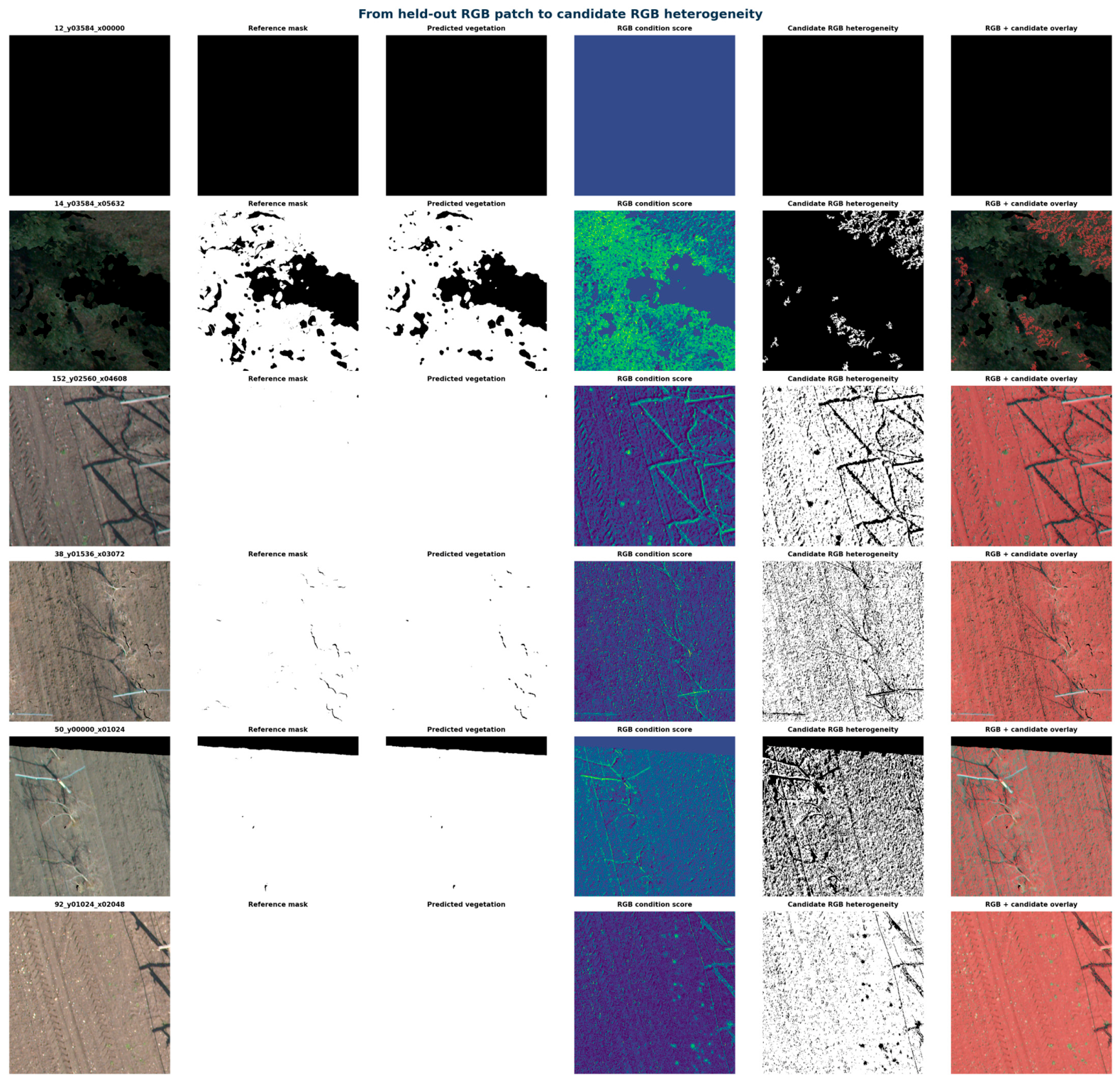
Representative examples of the complete processing sequence are shown in Figure 13. The figure presents the original RGB image patches, reference vegetation masks, predicted vegetation masks, RGB-based condition scores, candidate RGB heterogeneity masks, and overlays of the detected regions on the original imagery. The selected examples illustrate agricultural scenes with different vegetation structures and background conditions, consistent with the mixed composition of the experimental dataset. The results demonstrate that the proposed approach can localize spatial heterogeneity within segmented vegetation regions, including areas with complex geometry and uneven spatial distribution. The detected regions represent RGB-based canopy color heterogeneity and should not be interpreted as diagnoses of specific physiological crop stress.

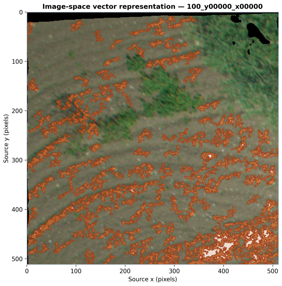
As shown in

Table 12. Spatial characteristics of automatically detected candidate RGB heterogeneity zones.

Zone ID	Source Image	Area (pixels)	Area (%)	Centroid (x, y)	Bounding Box (xmin, ymin, xmax, ymax)
c91_stress_1	c91	36	0.055	(114.8, 2.4)	(1646, 2048, 1655, 2056)
c91_stress_2	c91	34	0.052	(252.6, 2.7)	(1786, 2048, 1792, 2055)
c91_stress_3	c91	142	0.217	(101.5, 58.4)	(1633, 2090, 1642, 2124)
c91_stress_4	c91	4731	7.219	(219.2, 103.4)	(1681, 2093, 1792, 2217)
c91_stress_5	c91	12,740	19.440	(58.4, 184.3)	(1536, 2146, 1701, 2304)

, the detected candidate RGB heterogeneity regions were converted into image-space vector objects characterized by pixel area, centroid coordinates, contour geometry, and bounding boxes. All coordinates refer to the source-image pixel coordinate system and therefore describe relative spatial location within the original RGB image rather than geographic position. In the revised full-data analysis, 58,206 candidate RGB heterogeneity zones were generated. These objects provide a structured representation for subsequent image-space analysis but are not treated as georeferenced GIS polygons.

The results demonstrate that high-resolution RGB imagery can be used to identify and spatially characterize variations in vegetation appearance. The detected candidate RGB heterogeneity zones represent screening targets for subsequent field verification and should not be interpreted as physiologically confirmed crop-stress areas.

After the automatic detection of candidate RGB heterogeneity zones, the detected regions were converted into image-space vector objects and characterized by their pixel area, centroid coordinates, geometric boundaries, and bounding boxes. Figure 14 presents an example of this image-space vector representation, where the locations and relative sizes of individual zones are shown in the source-image pixel coordinate system. In the revised full-data analysis, the proposed algorithm identified 58,206 candidate RGB heterogeneity zones. These coordinates describe relative positions within the source UAV images and should not be interpreted as georeferenced geographic coordinates.

Figure 14 demonstrates the transformation of pixel-level segmentation outputs into image-space vector objects characterized by geometric parameters and relative spatial position. In the present Zenodo-based analysis, these objects remain in source-image pixel coordinates. Their transformation into georeferenced GIS objects would require georeferenced source imagery and a valid image-to-world transformation. The resulting image-space information is subsequently used for monitoring-priority assessment. Unlike traditional segmentation maps, the proposed approach not only locates problem areas but also provides their quantitative spatial characterization, which lays the foundation for automated planning of further field surveys and prioritization of agronomic measures.

3.6. Decision Support for Precision Crop Monitoring

In the final stage, the RGB-based indicators were integrated into the decision-support procedure defined by Equation (16). For each analyzed image patch, the Priority Score combined the normalized RGB heterogeneity share, the Mean RGB Appearance Score deficit, and the normalized number of candidate RGB heterogeneity zones with weights of 0.50, 0.30, and 0.20, respectively. According to Equation (17), the analyzed patches were classified into Low (P < 0.20), Medium (0.20 ≤ P < 0.45), and High (P ≥ 0.45) monitoring-priority classes.

The final decision-support analysis was performed on 3249 held-out image patches. Of these, 208 patches (6.40%) were classified as Low priority, 403 (12.40%) as Medium priority, and 2631 (80.98%) as High priority, while seven patches (0.22%) were not assigned a priority class. The resulting distribution is shown in Figure 15. These priority classes reflect the adopted heuristic Priority Score configuration and should be interpreted as screening categories for targeted visual or field verification rather than as agronomically validated intervention classes.

The Priority Score was also used to rank individual held-out image patches requiring the greatest attention during subsequent verification. As shown in Figure 15, the highest scores were obtained for patches 128_y01536_x03072 (0.7444), 92_y01536_x02048 (0.7331), 152_y01536_x04096 (0.7329), and 151_y01536_x04096 (0.7325). These high-ranking patches were characterized primarily by a large RGB heterogeneity share combined with a relatively low Mean RGB Appearance Score. Accordingly, the ranking identifies image regions for prioritized visual or field verification and should not be interpreted as evidence of physiologically confirmed crop stress or as a direct recommendation for agronomic treatment.

The quantitative characteristics of the highest-ranked image patches are presented in

Table 13. Characteristics of the highest-ranked UAV image patches identified by the RGB-based decision-support procedure.

Rank	UAV Image Patch ID	RGB Heterogeneity Share (%)	Mean RGB Appearance Score	Detected Candidate RGB Heterogeneity Zones	Priority Score	Recommended Action
1	128_y01536_x03072	94.54	0.1176	2	0.7444	Prioritize visual verification; no treatment diagnosis
2	92_y01536_x02048	94.56	0.1440	1	0.7331	Prioritize visual verification; no treatment diagnosis
3	152_y01536_x04096	93.16	0.1331	2	0.7329	Prioritize visual verification; no treatment diagnosis
4	151_y01536_x04096	92.61	0.1370	3	0.7325	Prioritize visual verification; no treatment diagnosis
5	152_y00000_x03584	93.94	0.1370	1	0.7321	Prioritize visual verification; no treatment diagnosis
6	281_y02048_x02560	91.89	0.1170	1	0.7279	Prioritize visual verification; no treatment diagnosis
7	281_y01536_x03072	91.81	0.1231	1	0.7256	Prioritize visual verification; no treatment diagnosis
8	128_y01024_x03072	92.02	0.1272	1	0.7254	Prioritize visual verification; no treatment diagnosis
9	136_y00000_x03072	94.12	0.1660	1	0.7243	Prioritize visual verification; no treatment diagnosis
10	152_y01024_x04096	91.71	0.1389	2	0.7239	Prioritize visual verification; no treatment diagnosis

. For each patch, the RGB heterogeneity share, Mean RGB Appearance Score, number of detected candidate RGB heterogeneity zones, and integrated Priority Score were determined. These indicators provide a structured basis for ranking image patches according to monitoring priority and identifying areas that warrant targeted visual or field verification.

Table 13 shows that the highest Priority Scores were generally associated with a high RGB heterogeneity share combined with a relatively low Mean RGB Appearance Score. The number of detected zones also contributed to the integrated ranking, although the highest-ranked patches were not necessarily those containing the largest number of individual zones. Thus, the proposed procedure performs a multi-criteria prioritization rather than ranking image patches according to a single indicator. Because the Priority Score is based on heuristic RGB-derived parameters, the resulting ranking should be interpreted as a screening tool for targeted visual or field verification and not as evidence of physiologically confirmed crop stress or as a direct recommendation for agronomic treatment.

The proposed approach extends conventional semantic segmentation by integrating RGB-based heterogeneity analysis, image-space vectorization, and monitoring-priority assessment. U-Net-ResNet50 was selected under the repeated source-image-grouped evaluation protocol and subsequently used for the spatial-analysis stage. The final full-data analysis generated 58,206 candidate RGB heterogeneity zones across 3249 held-out image patches. The resulting priority ranking provides structured screening information for targeted verification rather than a direct diagnosis of crop stress or a treatment recommendation.

3.7. Sensitivity Analysis of the Decision-Support Parameters

The sensitivity analysis showed that the decision-support ranking was relatively stable under moderate perturbations of most baseline parameters, although several components had a stronger influence on the results. Equal weighting of VARI, ExG, and GLI produced a Spearman correlation of 0.9914 with the baseline ranking, with only 1.0% of patches changing priority class. Changing the priority boundaries to 0.15/0.40 or 0.25/0.50 preserved the Priority Score ranking completely (ρ = 1.000), while changing the assigned priority class for 4.0% and 7.5% of patches, respectively.

The RGB heterogeneity threshold had a greater influence. Thresholds of 0.25, 0.35, and 0.40 produced rank correlations of 0.8476, 0.9486, and 0.9159, respectively, whereas the more pronounced reduction to 0.20 yielded ρ = 0.8331 and changed the priority class of 25.0% of patches. Removal of the RGB heterogeneity-share component from the Priority Score caused the largest ranking change (ρ = 0.0545; top-20 Jaccard = 0), demonstrating that this component has a dominant influence on prioritization. In contrast, removal of the RGB appearance-deficit or zone-count components retained substantially higher rank agreement (ρ = 0.9901 and 0.9382, respectively). Patch-local normalization also substantially altered the results (ρ = 0.2735; 42.0% priority-class changes), supporting the use of fixed training-derived normalization in the primary analysis.

To quantify the robustness of the heuristic decision-support formulation, the baseline parameters were systematically perturbed, and the resulting rankings were compared with the reference configuration. The main sensitivity results are summarized in

Table 14. Sensitivity of the decision-support procedure to selected parameter perturbations.

Scenario	Spearman ρ	Top-20 Jaccard	Changed Priority Class
Baseline	1.0000	1.0000	0.0%
Threshold = 0.20	0.8331	0.1111	25.0%
Threshold = 0.25	0.8476	0.4286	10.5%
Threshold = 0.35	0.9486	0.6667	3.5%
Threshold = 0.40	0.9159	0.5385	4.5%
Equal RGB-index weights	0.9914	0.8182	1.0%
Without heterogeneity share	0.0545	0.0000	10.0%
Without RGB appearance deficit	0.9901	0.9048	14.0%
Without zone count	0.9382	0.7391	6.0%
Priority cuts 0.15/0.40	1.0000	1.0000	4.0%
Priority cuts 0.25/0.50	1.0000	1.0000	7.5%
Patch-local normalization	0.2735	0.0526	42.0%

.

The normalization strategy was additionally evaluated by replacing the fixed training-derived bounds with the original patch-local normalization. This substantially altered the decision-support results (Spearman ρ = 0.2735, top-20 Jaccard = 0.0526, and 42.0% of priority classifications changed), confirming that patch-local normalization introduces considerable instability. Therefore, fixed training-derived normalization was retained for the final analysis.

The results show that moderate changes in most parameter settings preserved the overall ranking structure, whereas the RGB heterogeneity threshold, removal of the heterogeneity-share component, and patch-local normalization produced the largest deviations from the baseline. This confirms that the proposed Priority Score should be interpreted as an exploratory screening tool rather than as an agronomically calibrated decision rule.

Figure 16 shows that moderate perturbations of most parameters preserve the overall ranking structure, whereas the RGB heterogeneity threshold, removal of the heterogeneity-share component, and patch-local normalization have the strongest influence on the resulting priorities. Accordingly, the proposed Priority Score is retained as an exploratory screening metric rather than an agronomically calibrated decision rule.

4. Discussion

The results demonstrate three principal capabilities of the proposed framework. First, UAV RGB images can be segmented at the pixel level using deep learning models with satisfactory accuracy under the investigated conditions. Second, RGB-based indicators can reveal spatial heterogeneity within segmented vegetation areas, although these patterns should be interpreted only as proxy indicators of potential stress rather than as evidence of a specific physiological disorder. Third, the derived spatial indicators can be integrated into a multi-criteria procedure for prioritizing areas that require subsequent field inspection.

The experimental part was based on the open dataset «High-Resolution RGB Images and Corresponding Masks of Agricultural Fields,» acquired using a DJI Air 2S and compiled for several types of agricultural land, including green wheat crops [42]. The use of an open dataset is a key advantage of this work, as it ensures the reproducibility of the procedures for generating patches, training models, and verifying results.

Dividing the source material into 21,324 fragments measuring 512 × 512 pixels allowed us to standardize the input data while preserving sufficient local detail. Source-image-based separation of the training, validation, and test subsets reduced the risk of spatial information leakage that could otherwise occur if adjacent patches from the same source image were randomly distributed across different subsets. A similar dependence of accuracy on spatial imaging conditions, terrain, flight altitude, and scene structure has also been observed in other UAV studies. In particular, Zhu et al. demonstrated that changes in flight altitude affect the spatial resolution and accuracy of wheat biomass estimation, while Li et al. identified significant differences in plant segmentation accuracy between flat and topographically complex areas [44,45].

The repeated full-data comparison showed that U-Net-ResNet50 achieved the highest validation and held-out segmentation performance under the adopted experimental protocol. Across the three held-out test subsets, U-Net-ResNet50 achieved mean Precision = 0.9946 ± 0.0008, Recall = 0.9931 ± 0.0021, vegetation IoU = 0.9877 ± 0.0020, and Dice = 0.9938 ± 0.0010. FCN-ResNet50 and DeepLabV3-ResNet50 also demonstrated high segmentation performance, but their mean vegetation IoU values were lower [45,46,47,48]. These results characterize performance under the present experimental conditions and should not be interpreted as evidence of universal architectural superiority.

The repeated source-image-grouped experiments were complemented by independent external validation using DJI Mavic 3 Multispectral RGB imagery acquired over a wheat field. Without retraining or fine-tuning, U-Net-ResNet50 achieved Precision = 0.9323 ± 0.0009, Recall = 0.9221 ± 0.0045, vegetation IoU = 0.9115 ± 0.0060, and Dice = 0.9214 ± 0.0070. The decrease relative to the internal held-out evaluation is consistent with a domain shift associated with differences in UAV platform, sensor characteristics, illumination, and scene structure. These results provide preliminary evidence of cross-platform transferability; however, broader validation across additional fields, growing seasons, phenological stages, and acquisition conditions remains necessary [46,49].

A visual analysis of the FCN’s predictions showed that the model reproduced large, continuous areas of vegetation cover with sufficient accuracy, but could miss small or ambiguous fragments. This is consistent with the Precision = 0.8824 and Recall = 0.7713 metrics: the model was less likely to incorrectly classify the background as vegetation, but failed to detect some of the target pixels. Such errors in UAV segmentation are often associated with shadows, bare soil, variations in crop density, small plants, weeds, and textural similarities between neighboring classes. In the study by Li et al., small plants and weeds were among the main causes of segmentation omissions, while Wieme et al. emphasized the need for multi-year field data and a wide range of real-world scenes to ensure model robustness [45,49].

Another contribution of this work is the transition from binary vegetation segmentation to RGB-based spatial interpretation. The predicted vegetation masks were used to identify candidate RGB heterogeneity zones reflecting variations in canopy color and visible appearance. In the revised full-data analysis, 58,206 candidate RGB heterogeneity zones were converted into image-space vector objects characterized by pixel area, centroid coordinates, geometric boundaries, and bounding boxes. This demonstrates that pixel-level model outputs can be transformed into structured spatial information suitable for subsequent monitoring-priority assessment. Because the experimental Zenodo imagery was not georeferenced, the resulting objects are expressed in source-image pixel coordinates; their integration with GIS-based workflows would require georeferenced source imagery and a valid image-to-world transformation.

An important limitation is that the vectorized heterogeneity zones obtained from the open RGB dataset remain in source-image pixel coordinates. Consequently, the present computational experiment demonstrates image-space vectorization rather than a fully georeferenced GIS workflow. Transformation into a projected coordinate reference system, such as EPSG:32635, requires georeferenced source imagery and a valid image-to-world affine transformation. This functionality is therefore considered a subsequent deployment step rather than an experimentally validated component of the present dataset analysis.

At the same time, the term «potential stress zone» should be used with caution in this study. The VARI index and the derived RGB Appearance Score reflect differences in the color and structure of vegetation cover, but a similar visual signal may be caused by water deficit, insufficient nitrogen supply, disease, weed infestation, sparse planting, shading, or changes in light conditions. The study by Dong et al. confirms the effectiveness of UAV systems for detecting water stress, but such systems rely on specifically selected spectral, thermal, or structural features and field reference measurements [50]. Similarly, Wieme et al. used field-validated symptoms to train a system for detecting Alternaria solani, whereas the current dataset lacks reference labels for a specific physiological stress [49]. Therefore, the generated maps should be interpreted as maps of candidate areas for verification, rather than as maps of confirmed disease or nutrient deficiency.

A comparison with multimodal studies also points to directions for further improvement. Combining RGB and NIR data–or full multispectral data–allows for the simultaneous consideration of both textural-structural and physiological characteristics of vegetation. In the AgriFusion model, RGB–NIR multimodal fusion was used specifically to enhance semantic segmentation of complex agricultural scenes [51]. The primary model-development and architecture-comparison results were obtained using the open DJI Air 2S RGB dataset, whereas the DJI Mavic 3 Multispectral imagery was used separately for independent external field validation of the selected U-Net-ResNet50 model. The external experiment therefore complements, rather than replaces, the repeated internal evaluation and provides preliminary evidence of model transferability across UAV platforms and field-acquisition conditions.

In the final full-data decision-support analysis, 208 of the 3249 held-out image patches were classified as Low priority, 403 as Medium priority, and 2631 as High priority, while seven patches were not assigned a priority class. The ranking integrates RGB heterogeneity share, RGB Appearance Score deficit, and spatial fragmentation. Because these components remain heuristic and have not been agronomically calibrated, the resulting classes should be interpreted as relative monitoring priorities rather than direct indicators of crop treatment requirements.

The weights used in the Priority Score and the thresholds defining the Low, Medium, and High priority classes were heuristically specified for the proof-of-concept decision-support module and have not yet been independently validated against agronomic field observations. Future field validation should therefore assess these weights and thresholds using ground observations, agronomic measurements, and independently verified crop-condition data. Without such verification, the «Immediate field inspection» recommendation is justified as a monitoring measure, but not as an automatic decision regarding the application of fertilizers, pesticides, or irrigation. This aligns with the general logic of modern UAV research, where remote zoning is used for targeted plot selection, and the final diagnosis is confirmed by field measurements [49,50].

A further limitation concerns the spatial independence of the evaluation data. Grouping all patches from the same source UAV image within a single subset substantially reduces direct leakage between training and evaluation data, but it does not exclude possible spatial overlap between different source images, particularly when consecutive UAV frames were acquired with substantial forward or side overlap. Because verified field, flight, or non-overlapping geospatial-block identifiers were not available for the open dataset, a strict field-level or geospatial-block-level split could not be reconstructed. Consequently, the present results should be interpreted as source-image-grouped generalization rather than fully independent field-level generalization. Future validation should employ field-level or explicitly non-overlapping geospatial-block splits using independently acquired UAV datasets.

Future research should focus on five interrelated tasks. First, the models should be externally validated using UAV imagery acquired from independent fields, growing seasons, phenological stages, and imaging conditions, preferably using field-level or explicitly non-overlapping geospatial-block splits. Second, RGB imagery should be complemented with Red Edge and NIR channels, thermal data, and field measurements of moisture, nitrogen status, and disease symptoms. Third, source-image pixel coordinates should be transformed into georeferenced coordinates using valid GeoTIFF metadata or an image-to-world transformation to enable subsequent integration with GIS platforms. Fourth, predictive uncertainty should be quantified and incorporated into the decision-support procedure to avoid overconfident recommendations in ambiguous regions. Fifth, the weights and thresholds of the integrated priority index should be calibrated and validated using field observations and the economic consequences of intervention.

Beyond segmentation accuracy, a key contribution of this study is the implementation of an end-to-end workflow linking UAV RGB imagery, semantic segmentation, RGB-based heterogeneity analysis, image-space vectorization, and monitoring-priority assessment. This integration demonstrates the potential of the proposed system to reduce the scope of comprehensive field surveys and to target resources toward the most heterogeneous areas. At the same time, an agronomically specific interpretation of crop stress requires multispectral or thermal data and field validation; therefore, the current version of the system should be considered a screening and prioritization tool rather than a standalone method for definitive agronomic diagnosis.

5. Conclusions

This study developed and computationally validated an intelligent framework for automated crop monitoring that integrates UAV imagery, computer vision methods, deep learning models, RGB-based spatial analysis, and decision-support tools within a unified information workflow for precision agriculture. Unlike traditional approaches, the proposed system provides a full data processing cycle—from the analysis of UAV images to the generation of spatially localized recommendations for field monitoring.

Experimental validation was conducted using a mixed agricultural UAV RGB dataset under a repeated source-image-grouped full-data evaluation protocol. Among the evaluated architectures, U-Net-ResNet50 achieved the highest held-out performance, with mean Precision = 0.9946 ± 0.0008, Recall = 0.9931 ± 0.0021, vegetation IoU = 0.9877 ± 0.0020, and Dice = 0.9938 ± 0.0010, and was therefore selected for subsequent RGB-based spatial analysis.

Independent external validation using DJI Mavic 3 Multispectral RGB imagery acquired over a wheat field, without additional retraining or fine-tuning, yielded Precision = 0.9323 ± 0.0009, Recall = 0.9221 ± 0.0045, vegetation IoU = 0.9115 ± 0.0060, and Dice = 0.9214 ± 0.0070. These results provide preliminary evidence of cross-platform model transferability under the tested field conditions.

The developed framework transforms vegetation-segmentation outputs into candidate RGB heterogeneity zones, represents them as image-space vector objects, and integrates the resulting indicators into a monitoring-priority assessment. The final full-data spatial analysis generated 58,206 candidate RGB heterogeneity zones. These regions represent visible canopy heterogeneity and should not be interpreted as diagnoses of specific physiological crop stress.

The main limitations concern the use of software-generated reference masks in the open dataset, possible spatial overlap between different source UAV images, the absence of georeferencing metadata for the Zenodo imagery, and the heuristic nature of the RGB-based decision-support parameters. Although the independent Mavic 3M experiment provides preliminary external validation, broader field-level validation across additional crops, fields, seasons, and imaging conditions, together with multispectral or thermal data and field-based agronomic measurements, is required before operational deployment.

A further limitation concerns the reference masks supplied with the open dataset. These masks were generated using image-processing software rather than independently delineated by agronomic experts. Consequently, residual labeling uncertainty may remain, particularly along vegetation boundaries and in visually ambiguous regions. The reported segmentation metrics should therefore be interpreted as agreement with the supplied reference masks rather than as agreement with definitive biological ground truth. Independent expert annotation or field-validated reference data would be required for a stricter assessment of absolute segmentation accuracy.

The main limitations concern the use of software-generated reference masks, the absence of independent agronomic validation, possible spatial overlap between different source UAV images, and the lack of georeferencing metadata for the open RGB dataset. Future work should therefore focus on external field-level validation, multimodal UAV imagery, georeferenced spatial outputs, uncertainty quantification, and field-based calibration of the decision-support parameters.

References

1. Gamboa-Cruzado, J.; Estrada-Gutierrez, J.; Bustos-Romero, C.; Rivero, C.A.; Valenzuela, J.N.; Romero, C.A.T.; Gamarra-Moreno, J.; Amayo-Gamboa, F. A Review of Drones in Smart Agriculture: Issues, Models, Trends, and Challenges. Sustainability 2026, 18, 507. [Google Scholar] [CrossRef] [Scilit]
2. Silva, J.A.O.S.; Siqueira, V.S.; Mesquita, M.; Vale, L.S.R.; Silva, J.L.B.; Silva, M.V.; Lemos, J.P.B.; Lacerda, L.N.; Ferrarezi, R.S.; Oliveira, H.F.E. Artificial Intelligence Applied to Support Agronomic Decisions for the Automatic Aerial Analysis Images Captured by UAV: A Systematic Review. Agronomy 2024, 14, 2697. [Google Scholar] [CrossRef] [Scilit]
3. Ariza-Sentís, M.; Vélez, S.; Martínez-Peña, R.; Baja, H.; Valente, J. Object Detection and Tracking in Precision Farming: A Systematic Review. Comput. Electron. Agric. 2024, 219, 108757. [Google Scholar] [CrossRef] [Scilit]
4. Syrotiuk, V.; Syrotyuk, S.; Ptashnyk, V.; Tryhuba, A.; Baranovych, S.; Giełzecki, J.; Jakubowski, T. A Hybrid System with Intelligent Control for the Processes of Resource and Energy Supply of a Greenhouse Complex with Application of Energy Renewable Sources. Przegląd Elektrotechniczny 2020, 96, 149–152. [Google Scholar] [CrossRef] [Scilit]
5. Konieczna, A.; Padyuka, R.; Tryhuba, A.; Lub, P.; Ptashnyk, V.; Borek, K.; Rygało-Galewska, A.; Dybek, B.; Anders, D.; Klimek, K.; et al. Improving the Efficiency of Computer Networks Based on the Use of Seamless Wi-Fi Technology—The Use of Artificial Intelligence for Sustainable Agriculture. Appl. Sci. 2026, 16, 7916. [Google Scholar] [CrossRef] [Scilit]
6. Tryhuba, A.; Padyuka, R.; Tymochko, V.; Lub, P. Mathematical Model for Forecasting Product Losses in Crop Production Projects. CEUR Workshop Proc. 2022, 3109, 25–31. [Google Scholar]
7. Liu, X.; Luo, Z.; Yang, W.; Yuan, Y.; Gou, R. Semantic Segmentation of Agricultural Images: A Survey. Inf. Process. Agric. 2024, 11, 172–186. [Google Scholar] [CrossRef] [Scilit]
8. Epifani, L.; Caruso, A. A Survey on Deep Learning in UAV Imagery for Precision Agriculture and Wild Flora Monitoring: Datasets, Models and Challenges. Smart Agric. Technol. 2024, 9, 100625. [Google Scholar] [CrossRef] [Scilit]
9. Makam, S.; Komatineni, B.K.; Meena, S.S.; Meena, U. Unmanned Aerial Vehicles (UAVs): An Adoptable Technology for Precise and Smart Farming. Discov. Internet Things 2024, 4, 12. [Google Scholar] [CrossRef] [Scilit]
10. Guebsi, R.; Mami, S.; Chokmani, K. Drones in Precision Agriculture: A Comprehensive Review of Applications, Technologies, and Challenges. Drones 2024, 8, 686. [Google Scholar] [CrossRef] [Scilit]
11. Tsouros, D.C.; Bibi, S.; Sarigiannidis, P.G. A Review on UAV-Based Applications for Precision Agriculture. Information 2019, 10, 349. [Google Scholar] [CrossRef] [Scilit]
12. Kamilaris, A.; Prenafeta-Boldú, F.X. Deep Learning in Agriculture: A Survey. Comput. Electron. Agric. 2018, 147, 70–90. [Google Scholar] [CrossRef] [Scilit]
13. Maddikunta, P.K.R.; Hakak, S.; Alazab, M.; Bhattacharya, S.; Gadekallu, T.R.; Khan, W.Z.; Pham, Q.-V. Unmanned Aerial Vehicles in Smart Agriculture: Applications, Requirements, and Challenges. IEEE Sens. J. 2021, 21, 17608–17619. [Google Scholar] [CrossRef] [Scilit]
14. Chettri, K.; Sen, B.; Ghosal, P. Deep Learning for Precision Agriculture: A Systematic Review of Methods, Challenges, and Future Directions. Knowl. Inf. Syst. 2026, 68, 35. [Google Scholar] [CrossRef] [Scilit]
15. Lei, L.; Yang, Q.; Yang, L.; Shen, T.; Wang, R.; Fu, C. Deep Learning Implementation of Image Segmentation in Agricultural Applications: A Comprehensive Review. Artif. Intell. Rev. 2024, 57, 149. [Google Scholar] [CrossRef] [Scilit]
16. Bae, W.D.; Alkobaisi, S.; Safdar, M.F.; Chouhan, P. A Taxonomy of Machine Learning for UAV-Enabled Precision Agriculture: A Structured Survey. AgriEngineering 2026, 8, 249. [Google Scholar] [CrossRef] [Scilit]
17. Saha, S.; Ghose, D.; Konar, A.; Nagar, A.K. Machine Learning for Precision Agriculture Using Imagery from Unmanned Aerial Vehicles (UAVs): A Survey. Drones 2023, 7, 382. [Google Scholar] [CrossRef] [Scilit]
18. Wang, D.; Zhao, M.; Li, Z.; Xu, S.; Wu, X.; Ma, X.; Liu, X. A Survey of Unmanned Aerial Vehicles and Deep Learning in Precision Agriculture. Eur. J. Agron. 2024, 161, 127477. [Google Scholar] [CrossRef] [Scilit]
19. Liu, J.; Xiang, J.; Jin, Y.; Liu, R.; Yan, J.; Wang, L. Boost Precision Agriculture with Unmanned Aerial Vehicle Remote Sensing and Edge Intelligence: A Survey. Remote Sens. 2021, 13, 4387. [Google Scholar] [CrossRef] [Scilit]
20. Xu, F.; Yao, X.; Zhang, K.; Yang, H.; Feng, Q.; Li, Y.; Yan, S.; Gao, B.; Li, S.; Yang, J.; et al. Deep Learning in Cropland Field Identification: A Review. Comput. Electron. Agric. 2024, 222, 109042. [Google Scholar] [CrossRef] [Scilit]
21. Osco, L.P.; Marcato Junior, J.; Ramos, A.P.M.; de Castro Jorge, L.A.; Fatholahi, S.N.; de Andrade Silva, J.; Matsubara, E.T.; Pistori, H.; Gonçalves, W.N.; Li, J. A Review on Deep Learning in UAV Remote Sensing. Int. J. Appl. Earth Obs. Geoinf. 2021, 102, 102456. [Google Scholar] [CrossRef] [Scilit]
22. Wu, X.; Li, W.; Hong, D.; Tao, R.; Du, Q. Deep Learning for UAV-Based Object Detection and Tracking: A Survey. Remote Sens. 2022, 14, 1370. [Google Scholar] [CrossRef] [Scilit]
23. Dalal, M.; Mittal, P. A Systematic Review of Deep Learning-Based Object Detection in Agriculture: Methods, Challenges, and Future Directions. Comput. Mater. Contin. 2025, 84, 57–91. [Google Scholar] [CrossRef] [Scilit]
24. Charisis, C.; Argyropoulos, D. Deep Learning-Based Instance Segmentation Architectures in Agriculture: A Review of the Scopes and Challenges. Smart Agric. Technol. 2024, 8, 100448. [Google Scholar] [CrossRef] [Scilit]
25. Dobosz, B.; Gozdowski, D.; Koronczok, J.; Žukovskis, J.; Wójcik-Gront, E. Deep Learning Segmentation Models for UAV-Based Detection of Crop Damage in Rapeseed Using RGB Imagery. Agriculture 2026, 16, 536. [Google Scholar] [CrossRef] [Scilit]
26. Gao, J.; Liao, W.; Nuyttens, D.; Lootens, P.; Xue, W.; Alexandersson, E.; Pieters, J. Cross-Domain Transfer Learning for Weed Segmentation and Mapping in Precision Farming Using Ground and UAV Images. Expert Syst. Appl. 2024, 246, 122980. [Google Scholar] [CrossRef] [Scilit]
27. Cheng, J.; Zhu, Y.; Zhao, Y.; Li, T.; Chen, M.; Sun, Q.; Gu, Q.; Zhang, X. Application of an Improved U-Net with Image-to-Image Translation and Transfer Learning in Peach Orchard Segmentation. Int. J. Appl. Earth Obs. Geoinf. 2024, 130, 103871. [Google Scholar] [CrossRef] [Scilit]
28. Zheng, Z.; Yuan, J.; Yao, W.; Yao, H.; Liu, Q.; Guo, L. Crop Classification from Drone Imagery Based on Lightweight Semantic Segmentation Methods. Remote Sens. 2024, 16, 4099. [Google Scholar] [CrossRef] [Scilit]
29. Sandoval-Pillajo, L.; García-Santillán, I.; Pusdá-Chulde, M.; Giret, A. Weed Detection Based on Deep Learning from UAV Imagery: A Review. Smart Agric. Technol. 2025, 12, 101147. [Google Scholar] [CrossRef] [Scilit]
30. Tryhuba, I.; Tryhuba, A.; Grabovets, V.; Bodak, V.; Horodetska, N. Forecasting the Duration of Work in Plant Protection Projects. CEUR Workshop Proc. 2023, 3453, 96–105. [Google Scholar]
31. Tryhuba, A.; Kotenko, V. Intelligent Information System for Resource Planning in Grain Crops Delivery Projects on the Basis of Machine Learning. In 2023 IEEE 18th International Conference on Computer Science and Information Technologies (CSIT); IEEE: New York, NY, USA, 2023; pp. 1–4. [Google Scholar] [CrossRef] [Scilit]
32. Saini, P.; Nagesh, D.S. A Review of Deep Learning Applications in Weed Detection: UAV and Robotic Approaches for Precision Agriculture. Eur. J. Agron. 2025, 168, 127652. [Google Scholar] [CrossRef] [Scilit]
33. Kuan, Y.; Goh, K.; Lim, L. Systematic Review on Machine Learning and Computer Vision in Precision Agriculture: Applications, Trends, and Emerging Techniques. Eng. Appl. Artif. Intell. 2025, 148, 110401. [Google Scholar] [CrossRef] [Scilit]
34. Bazrafkan, A.; Igathinathane, C.; Bandillo, N.; Flores, P. Optimizing Integration Techniques for UAS and Satellite Image Data in Precision Agriculture—A Review. Front. Remote Sens. 2025, 6, 1622884. [Google Scholar] [CrossRef] [Scilit]
35. Xing, Y.; Liu, X.; Wang, X. Integrating UAVs, Satellite Remote Sensing, and Machine Learning in Precision Agriculture: Pathways to Sustainable Food Production, Resource Efficiency, and Scalable Innovation. Front. Agron. 2025, 7, 1670380. [Google Scholar] [CrossRef] [Scilit]
36. Buitrago Bolívar, E.; Rico Franco, J.A.; Rojas Amador, S. Crop and Soil Monitoring in Precision Agriculture with UAVs and Artificial Intelligence: A Review. Tecnura 2024, 28, 75–103. [Google Scholar] [CrossRef] [Scilit]
37. Kizielewicz, B.; Wątróbski, J.; Sałabun, W. Multi-criteria Decision Support System for the Evaluation of UAV Intelligent Agricultural Sensors. Artif. Intell. Rev. 2025, 58, 194. [Google Scholar] [CrossRef] [Scilit]
38. Kondysiuk, I.; Bashynsky, O.; Grabovets, V.; Dembitskyi, V.; Myskovets, I. Formation and Risk Assessment of Stakeholders Value of Motor Transport Enterprises Development Projects. In 2021 IEEE 16th International Conference on Computer Sciences and Information Technologies (CSIT); IEEE: New York, NY, USA, 2021; Volume 2, pp. 303–306. [Google Scholar] [CrossRef] [Scilit]
39. Mowla, M.N.; Mowla, N.; Chowdhury, S.R.; Rabie, K.M.; Shongwe, T. Unmanned Aerial Vehicles (UAVs) for Smart Agriculture with Machine Learning: A System-Oriented Review of Methods, Applications, and Challenges. Smart Agric. Technol. 2026, 13, 101880. [Google Scholar] [CrossRef] [Scilit]
40. Pu, X.; Yang, D.; Gong, C.; Zhu, F.; Zhou, R. Bridging Lab and Field: A Review and Roadmap for Unmanned Aerial Vehicle-Based Field Crop Counting with Deep Learning. Smart Agric. Technol. 2025, 12, 101639. [Google Scholar] [CrossRef] [Scilit]
41. Tryhuba, A.; Komarnitskyi, S.; Tryhuba, I.; Hutsol, T.; Yermakov, S.; Muzychenko, A.; Muzychenko, T.; Horetska, I. Planning and Risk Analysis in Projects of Procurement of Agricultural Raw Materials for the Production of Environmentally Friendly Fuel. Int. J. Renew. Energy Dev. 2022, 11, 569–580. [Google Scholar] [CrossRef] [Scilit]
42. Canistro, F.; De Marinis, P.; Vessio, G.; Castellano, G. High-Resolution RGB Images and Corresponding Masks of Agricultural Fields. Zenodo 2024. Version v1. [Google Scholar] [CrossRef]
43. Zhang, S.; Wang, X.; Lin, H.; Dong, Y.; Qiang, Z. A Review of the Application of UAV Multispectral Remote Sensing Technology in Precision Agriculture. Smart Agric. Technol. 2025, 12, 101406. [Google Scholar] [CrossRef] [Scilit]
44. Zhu, W.; Rezaei, E.E.; Nouri, H.; Sun, Z.; Li, J.; Yu, D.; Siebert, S. UAV Flight Height Impacts on Wheat Biomass Estimation via Machine and Deep Learning. IEEE J. Sel. Top. Appl. Earth Obs. Remote Sens. 2023, 16, 7471–7485. [Google Scholar] [CrossRef] [Scilit]
45. Li, Q.; Zhou, Z.; Qian, Y.; Yan, L.; Huang, D.; Yang, Y.; Luo, Y. Accurately Segmenting/Mapping Tobacco Seedlings Using UAV RGB Images Collected from Different Geomorphic Zones and Different Semantic Segmentation Models. Plants 2024, 13, 3186. [Google Scholar] [CrossRef] [Scilit]
46. Zhang, G.; Yan, H.; Zhang, D.; Zhang, H.; Cheng, T.; Hu, G.; Shen, S.; Xu, H. Enhancing Model Performance in Detecting Lodging Areas in Wheat Fields Using UAV RGB Imagery: Considering Spatial and Temporal Variations. Comput. Electron. Agric. 2023, 214, 108297. [Google Scholar] [CrossRef] [Scilit]
47. Azizi, A.; Zhang, Z.; Rui, Z.; Li, Y.; Igathinathane, C.; Flores, P.; Mathew, J.; Pourreza, A.; Han, X.; Zhang, M. Comprehensive Wheat Lodging Detection after Initial Lodging Using UAV RGB Images. Expert Syst. Appl. 2024, 238, 121788. [Google Scholar] [CrossRef] [Scilit]
48. Zhu, Q.; Wang, K.; Liang, D.; Tang, J. WLUSNet: A Lightweight Wheat Lodging Segmentation Network Based on UAV Image. Comput. Electron. Agric. 2025, 237, 110587. [Google Scholar] [CrossRef] [Scilit]
49. Wieme, J.; Leroux, S.; Cool, S.R.; Van Beek, J.; Pieters, J.G.; Maes, W.H. Ultra-High-Resolution UAV-Imaging and Supervised Deep Learning for Accurate Detection of Alternaria solani in Potato Fields. Front. Plant Sci. 2024, 15, 1206998. [Google Scholar] [CrossRef] [Scilit]
50. Dong, H.; Dong, J.; Sun, S.; Bai, T.; Zhao, D.; Yin, Y.; Shen, X.; Wang, Y.; Zhang, Z.; Wang, Y. Crop Water Stress Detection Based on UAV Remote Sensing Systems. Agric. Water Manag. 2024, 303, 109059. [Google Scholar] [CrossRef] [Scilit]
51. Li, X.; Qiao, L.; Yang, C. AgriFusion: Multiscale RGB–NIR Fusion for Semantic Segmentation in Airborne Agricultural Imagery. AgriEngineering 2025, 7, 388. [Google Scholar] [CrossRef] [Scilit]
Figure 1. Generalized architecture of intelligent crop monitoring systems based on UAV technologies and deep learning.
Applsci 16 09747 g001
Figure 2. Overall research framework of the intelligent UAV-based crop monitoring system, including data acquisition, data preparation, dataset development, deep learning analysis, and spatial decision support.
Applsci 16 09747 g002
Figure 3. Representative RGB images and corresponding reference masks from the mixed agricultural dataset used in the study.
Applsci 16 09747 g003
Figure 4. Proposed hardware architecture of the intelligent UAV-based crop monitoring system, including data acquisition, RTK positioning, onboard processing, and geospatial data analysis.
Applsci 16 09747 g004
Figure 5. Proposed UAV image preprocessing workflow, including radiometric correction, photogrammetric processing, orthomosaic generation, image tiling, normalization, and data augmentation prior to deep learning.
Applsci 16 09747 g005
Figure 6. Operational workflow of the proposed intelligent UAV-based crop monitoring system, including UAV image acquisition, preprocessing, semantic segmentation, RGB-based heterogeneity zone mapping, spatial analysis, and decision support.
Applsci 16 09747 g006
Figure 7. Automatic generation of 512 × 512 image patches from the source high-resolution UAV RGB images.
Applsci 16 09747 g007
Figure 8. Distribution of image patches among the training, validation, and test subsets for seeds 42, 123, and 2026.
Applsci 16 09747 g008
Figure 9. Pixel-level distribution of semantic classes in the experimental UAV dataset.
Applsci 16 09747 g009
Figure 10. Pilot field validation using the DJI Mavic 3 Multispectral: (a) UAV platform used for field acquisition; (b) representative RGB image acquired during the pilot flight; (c) spatially referenced image/orthomosaic obtained from the field acquisition.
Applsci 16 09747 g010
Figure 11. Training behavior of U-Net-ResNet50, DeepLabV3-ResNet50, and FCN-ResNet50 across the three repeated full-data experiments. The figure summarizes validation IoU and convergence characteristics for seeds 42, 123, and 2026. Diamonds indicate the best validation epoch, whereas bars indicate the total number of executed epochs.
Applsci 16 09747 g011
Figure 12. Repeated source-image-grouped comparison of the evaluated architectures: (a) validation vegetation IoU used exclusively for architecture selection; (b) vegetation IoU obtained on the held-out test subsets. Points represent individual repeats, while diamonds and error bars indicate mean values and standard deviations.
Applsci 16 09747 g012
Figure 13. RGB-based spatial interpretation of candidate canopy color heterogeneity in representative held-out agricultural vegetation patches. From left to right: original RGB patch, reference vegetation mask, predicted vegetation mask, RGB-based condition score, candidate RGB heterogeneity mask, and overlay of the detected heterogeneity regions on the original RGB image. In the RGB condition score maps, the color gradient represents relative variation in the calculated RGB-based condition score, while the colored overlay highlights candidate RGB heterogeneity regions detected within the predicted vegetation area.
Applsci 16 09747 g013
Figure 14. Representative image-space vectorization of candidate RGB heterogeneity zones. Detected regions are represented as vector contours in source-image pixel coordinates. The brown/orange contours indicate the boundaries of the detected candidate RGB heterogeneity zones, while the underlying image shows the original RGB patch. The coordinates are not georeferenced and do not correspond to a geographic coordinate reference system; transformation to GIS coordinates requires georeferenced source imagery and a valid image-to-world transformation.
Applsci 16 09747 g014
Figure 15. Decision-support results for the held-out image patches: (a) distribution of exploratory monitoring-priority classes; (b) twelve image patches with the highest heuristic Priority Scores. The resulting priorities are intended to support targeted visual or field verification and should not be interpreted as treatment recommendations or physiologically confirmed crop-stress diagnoses.
Applsci 16 09747 g015
Figure 16. One-at-a-time sensitivity and ablation analysis of the RGB-based decision-support procedure: (a) fraction of image patches changing priority class relative to the baseline; (b) Spearman rank correlation of Priority Scores with the baseline; and (c) Jaccard similarity of the top-20 priority sets.
Applsci 16 09747 g016