Unlocking Low-Carbon Heat: Geothermal Feasibility and Thermal Breakthrough in Carboniferous Sandstone Aquifers

Abstract

Decarbonisation is crucial for mitigating climate change, with ground source heat pumps (GSHPs) playing a key role in reducing reliance on gas for space heating. This study investigates the potential of an open-loop GSHP system in the Carboniferous Millstone Grit of Ilkley, West Yorkshire, using Ilkley Lido and surrounding sports facilities as an example heating demand. The feasibility of systems installed at depths less than 150 m is examined, considering both shallow and deeper geological conditions. Available data on subsurface geology, hydrogeology, and geothermal gradients are utilised to characterise the formations and target depths, with cross-sectional models developed to assess the potential. The Marchup Grit aquifer is identified as the primary target due to its relatively shallow depth (~90 m), expected subsurface temperature (~14.5 °C), and moderate transmissivity. Additional geothermal potential is also considered in the Warley Wise Grit and Pendleside Limestone. The study contrasts borehole and field data with literature findings, including measurements at outcrop level of the Marchup Grit. To assess the feasibility of an open-loop GSHP system, a doublet configuration is simulated, matching the estimated heat demand of the facilities. The results demonstrate that an open-loop doublet system is conditionally feasible within the Marchup Grit aquifer; however, long-term operational performance remains sensitive to thermal feedback (estimated at ~22 years analytically for a 300 m well spacing and 8–10 years numerically under a 130 m minimum spacing constraint at peak abstraction rates). By reducing abstraction to 70% of the peak heating demand, long-term sustainability can be improved. Overall, while the system exhibits preliminary potential, commercial implementation remains subject to confirmatory site-specific borehole drilling, hydrochemical sampling, and long-duration pumping tests to validate reservoir capacity and optimise system longevity.

1. Introduction

The benefits of utilising geothermal energy are clear, with a globally inexhaustible resource, low emission of CO₂ and other pollutants, stable base load of energy, and low lifetime costs, while some limitations need to be considered at an early stage in project development [1,2,3,4]. These include resource depletion at reservoir level, and high upfront cost and initial risk [5]. With thorough characterisation and assessment, these risks can be managed to reduce uncertainty, allowing efficient development of well systems.

Research into geothermal energy utilisation across the UK has naturally focused on those aquifers and regions that have the highest potential temperatures and flows, such as the coalfields of Britain [6,7], Carboniferous limestones [8], and Permo-Triassic sandstones [9]. However, great potential still exists in areas/aquifers outside of these identified resources for use on a smaller scale, and research should, therefore, attempt to assess the feasibility of these resources. This study assesses the feasibility of open-loop GSHP systems in the Carboniferous Millstone Grit of Ilkley and uses the estimated space heating requirements of Ilkley Lido and surrounding sports facilities as an example of a possible heating scenario.

Beyond evaluating local viability, this study establishes a transferable, multi-stage screening framework for de-risking low-enthalpy open-loop GSHP schemes within data-sparse, fractured, multilayered sedimentary basins. By synthesising legacy borehole records, multi-scale discontinuity logging, digital core thresholding, and coupled analytical–numerical thermal feedback simulations, this methodology demonstrates how sub-formation anisotropy and structural compartmentalisation can be pre-screened before committing capital to deep borehole drilling.

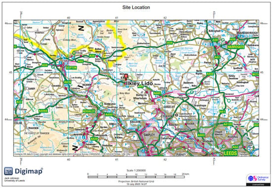
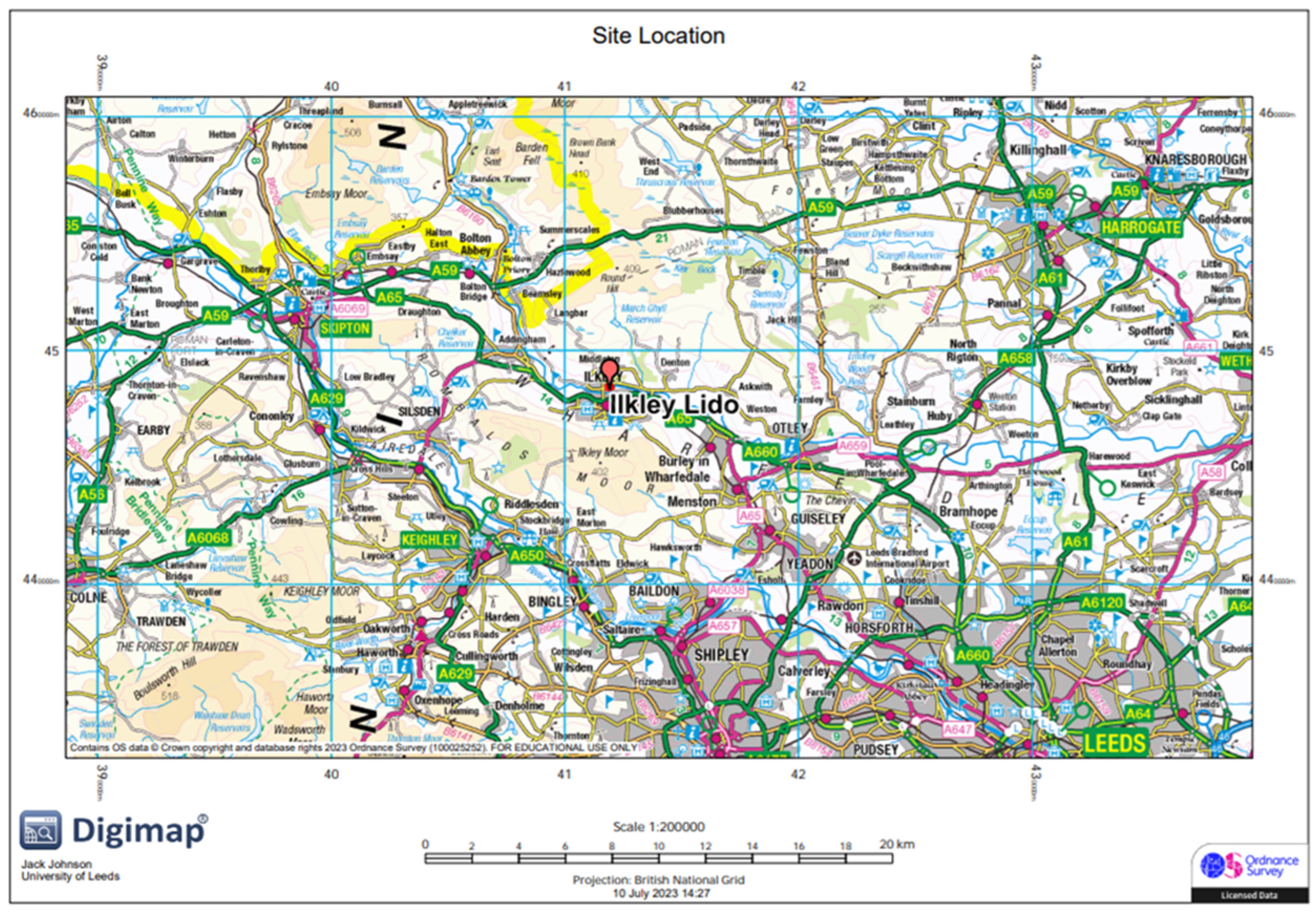
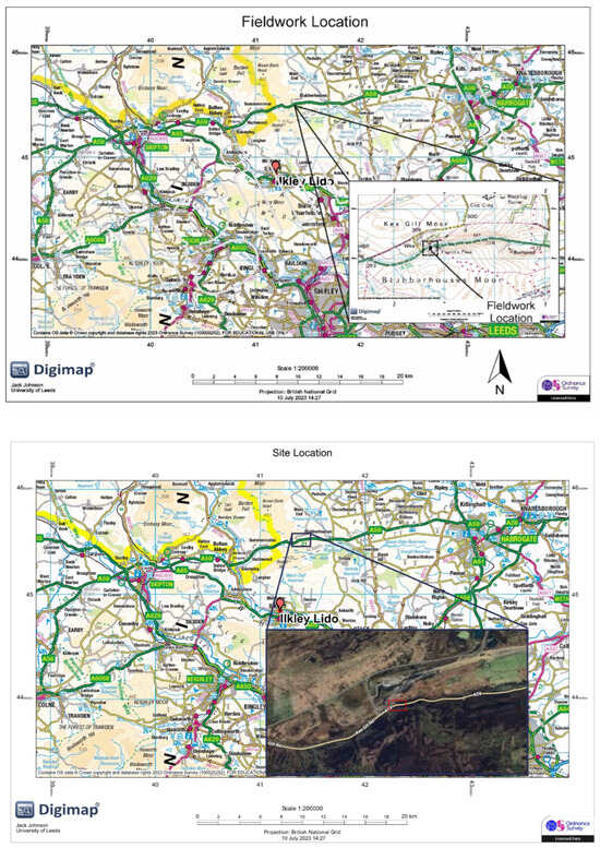
Ilkley Lido and the surrounding sports facilities (‘the study area’) are situated to the north of the River Wharfe in Ilkley, West Yorkshire, shown in Figure 1. The Lido has indoor and outdoor swimming facilities. The surrounding area comprises the sports facilities, with Ilkley Cricket Club within 250 m to the west and Ilkley Rugby Club within 250 m to the southwest. Residential land use dominates further west beyond the cricket club, and Ilkley town centre is around 800 m southwest.

Figure 1. Regional location map of the study area within Yorkshire [10]. The immediate site-specific boundary encompassing Ilkley Lido.

The study outlines key concepts through a literature review. Section 3 outlines the approach taken for data collection and processing. After this, a detailed outline of the study area and relevant information on the ground conditions are presented. Fieldwork was undertaken as part of the study and the data are presented following the outline of regional information. A conceptual ground model based upon the available information is presented, which is the basis of any geothermal well system. The heat demand of the facilities and pool heating is also estimated, which feeds into the feasibility assessment of geothermal systems. A discussion around the data and feasibility is then undertaken, which critically assesses the findings.

2. Background

A geothermal resource consists of a reservoir (aquifer) that holds a source of extractable heat, also termed as geothermal target, which is classified as low enthalpy (low temperature) at less than 150 °C, and mid–high enthalpy as above 150 °C (high temperature) [11]. Shallow geothermal resources tend to be low enthalpy, and deeper resources are high enthalpy due to the increase in temperature with geothermal gradient.

Hydraulic conductivity (permeability) and thermal conductivity are key properties in the propagation of heat in the subsurface. Therefore, high-porosity and high-permeability rocks and soils are the most suitable targets for geothermal heat extraction [11,12]. Heat transport in aquifers is driven by either convection (dominant in active, high-enthalpy systems) or conduction (dominant in passive, low–medium enthalpy) [12,13].

2.1. Ground Source Heat Pumps (GSHPs)

A GSHP can use the ground as a heat source or sink. The heat pump passes water over a low-boiling-point refrigerant, then compresses and superheats it. The increase in thermal energy is extracted via a heat exchanger for space heating via air or water, or the process can be run in reverse to achieve space cooling [12,14]. Energy is consumed in the operation of heat pumps to run heat exchangers and in ancillary processes. The operation of a heat pump in heating mode is characterised by the coefficient of performance (COP_h), which is defined as the ratio between the useful thermal energy (H) and the energy consumed to obtain it (E) in Equation (1) [14]:

$${\mathit{COP}}_h= {\displaystyle \frac{H}{E}}.$$

(1)

Increasing the input temperature and decreasing output temperature results in higher COP. Ideal COP values are between 3.0 and 4.0 under operational conditions [12].

The useful heating effect (H) of a GSHP can be calculated using Equation (2):

$$H = {\displaystyle \frac{Z x ∆\theta x S_{\mathit{VCwater}}}{\left(1-\frac{1}{{\mathit{COP}}_h}\right)}} ,$$

(2)

where Z is flow rate (Ls⁻¹), ∆θ is temperature drop across the heat pump, and S_VCwater is the specific heat capacity of water (4180 JL⁻¹K⁻¹).

Reversing the process can provide space cooling. The cooling effect, C (kW), can be calculated using Equation (3):

$$C = {\displaystyle \frac{Z x ∆\theta x S_{\mathit{VCwater}}}{\left(1+\frac{1}{{\mathit{COP}}_c}\right)}},$$

(3)

and Equation (4):

$$\mathit{COPc} = {\displaystyle \frac{C}{E}},$$

(4)

where COP_c is the coefficient of performance for a GSHP in cooling mode.

Design of abstraction wells in open-loop systems is dependent on the depth to aquifer, groundwater level, hydraulic conductivity, yield of the well, which determines the design diameter, and the lithology of the aquifer [11,12].

Heat extraction occurs through forced advection of groundwater rather than conduction, which results in higher rates of heat extraction when compared to closed-loop systems. However, the risk of clogging/fouling of heat exchangers is present, dependent on water chemistry and particulates [15]. A doublet arrangement is common with open-loop systems that utilises an abstraction well and a reinjection well. This can allow for increased well efficiency, increasing the sustainability of the system by stabilising pressures in the aquifer and increasing/stabilising yields from the abstraction well [16].

Closed-loop systems do not require the abstraction of water and can, therefore, be utilised practically anywhere that a temperature gradient exists. However, a higher upfront cost is usually associated with closed-loop borehole arrays due to the need for more boreholes to meet similar demands in open-loop systems [12].

2.2. Hydraulic and Thermal Feedback

In a doublet arrangement, reinjecting cooled water after abstraction may induce cool water flow back to the abstraction well, and this process is termed hydraulic feedback. Ref. [17] states this will occur when (Equation (5)):

$$L < {\displaystyle \frac{2Z}{\mathit{T\pi i}}},$$

(5)

where L is the borehole spacing (m), T is aquifer transmissivity (m²/day), Z is pumping rate (m³/day), and i is the natural hydraulic gradient. An estimate for the time it takes for breakthrough of the cooled water into the abstraction well can be made using Equation (6):

$$t_{\mathit{hyd}} = \pi n_{e}D{\displaystyle \frac{L^2}{3Z}} ,$$

(6)

where n_e is the effective porosity as a fraction, and D is the aquifer thickness (m). This does not account for fracture flow and assumes a low natural hydraulic gradient but can be assumed to be a worst-case scenario [12].

Thermal breakthrough times are slower than hydraulic breakthrough times because heat travels via conduction, exchange between groundwater and the aquifer matrix, and through advection of groundwater [12,18]. An estimate of thermal breakthrough times can be made using Equation (7), given by [12]:

$$t_{\mathit{the}}= \mathit{\pi D}{\displaystyle \frac{S_{\mathit{vcaq}}{L}^2}{3S_{\mathit{vcwat}}Z}},$$

(7)

where t_the is thermal breakthrough time, s_vcaq is the volumetric heat capacity of the aquifer, and s_vcwat is the volumetric heat capacity of water.

The analytical relationships formulated in Equations (5)–(7) assume an idealised, homogeneous, non-leaky 2D confined aquifer with uniform thickness, constant effective porosity, and steady-state planar regional flow. In structurally complex, multilayered basins, such as the Millstone Grit Group, localised fault throw, lithological interbedding, and discrete fracture networks violate pure Darcian homogeneity. Consequently, these closed-form equations cannot resolve preferential channelling or 3D thermal dissipation; instead, they serve as first-order analytical screening baselines that approximate worst-case, direct piston displacement advective breakthrough times.

3. Methodology and Area of Interest

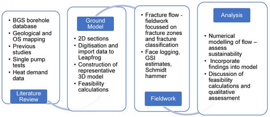
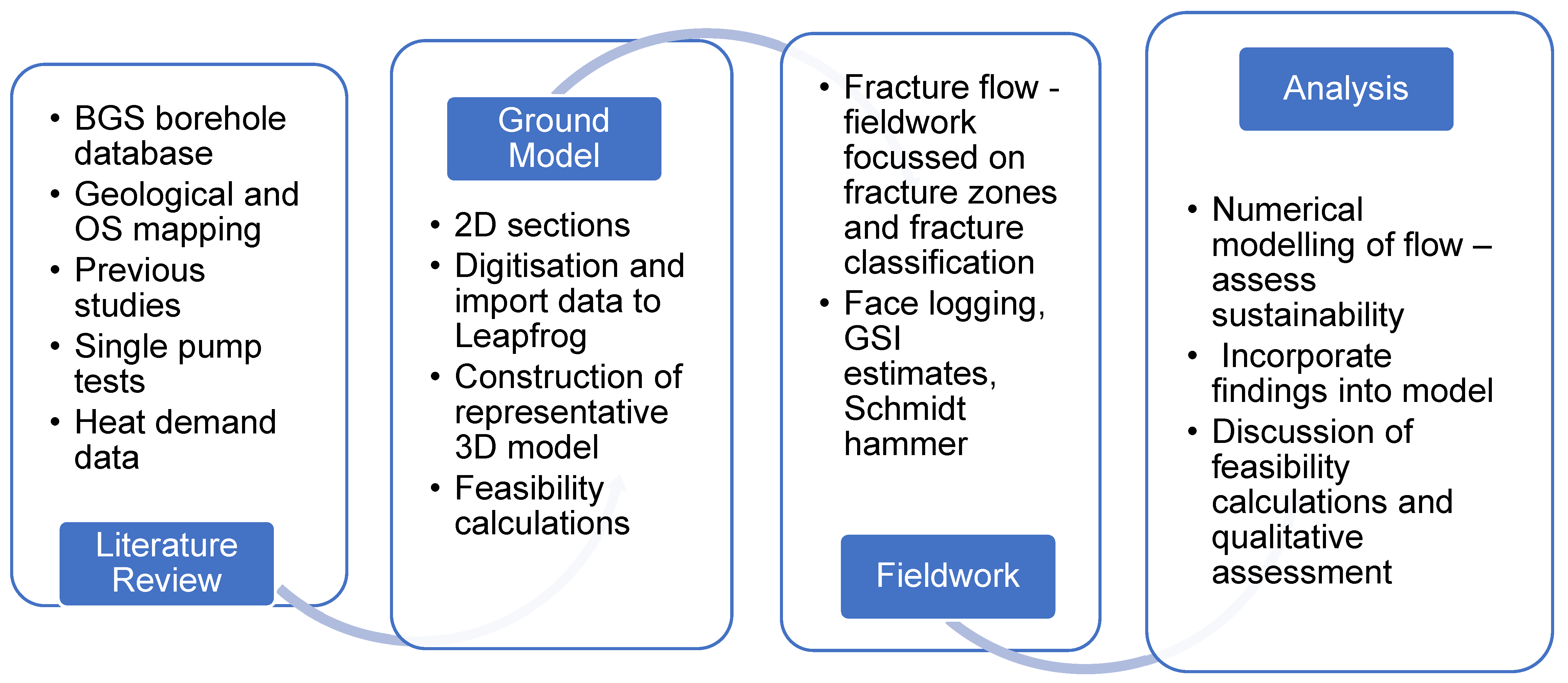
This study makes use of open-source data, with the main source of information being accessed through Ref. [19]. Figure 2 shows an outline of the approach to data collection and processing, the focus of fieldwork, and the process for analysing the data.

Figure 2. Flow chart showing the four key steps of the methodology developed and adopted in this research work (in chronological order from left to right).

The general approach to data collection and analysis for the study was guided by the World Bank Geothermal Handbook [5] and the Australian Geothermal Reporting Code [20].

Processing of pump test data was undertaken using the [21] straight line method. Cross-sections were built using BGS mapping and available sources, with data then imported into Leapfrog^® Geo 2023.1 software. A 3D model was built using these data and processed borehole data. Feasibility assessment was undertaken using the model as a frame of reference, the equations outlined in Section 2, and finally compared to a numerical model of flow to understand the sustainability in terms of thermal and hydraulic feedback to an open-loop system. Results from fieldwork were also incorporated, including logging in accordance with BS EN ISO 14689:2018 and BS5930:2015+A1:2020, Schmidt hammer testing according to the ISRM suggested method [22], and discontinuity surveys. Several hand samples were also taken to estimate the porosity of the target aquifer. Image analysis using ImageJ (v.1.54) software was also undertaken to estimate porosity through auto-thresholding of images to reduce user bias. Mean fracture spacing was calculated to estimate fracture permeability, and an average permeability including the matrix permeability.

3.1. Geological Setting and Stratigraphy

The geological setting of the study area is demonstrated in Figure 3, and lies to the south of the Askrigg Block, within the Huddersfield Basin [23]. The Carboniferous sequence is understood to rest on strongly deformed Lower Palaeozoic sediments at depth.

Figure 3. Showing the location of Ilkley in relation to structural features and geology at surface [23].

Crustal extension during the late Devonian and into the Dinantian resulted in formation of horst and graben structures trending east–northeast and displacement of hundreds of metres, during which time shallow marine carbonates and muds dominated the depositional system [24]. A major change in depositional environment occurred in the early Namurian (Upper Carboniferous) as clastic fluvio-deltaic conditions prevailed, which led to deposition of the Millstone Grit [25]. Regional post-extensional subsidence occurred concurrently with deposition of these sediments, and the estimated maximum thickness of the sediments is between 1.3 km and 1.6 km [24]. Deposition of coal measures then followed.

Following the Carboniferous, the Variscan Orogenic event caused basin inversion and reactivation/reversal of faulting along with folding. Some of the faulting is thought to relate to Dinantian transfer faults, with surface displacements in the tens of metres [23,24].

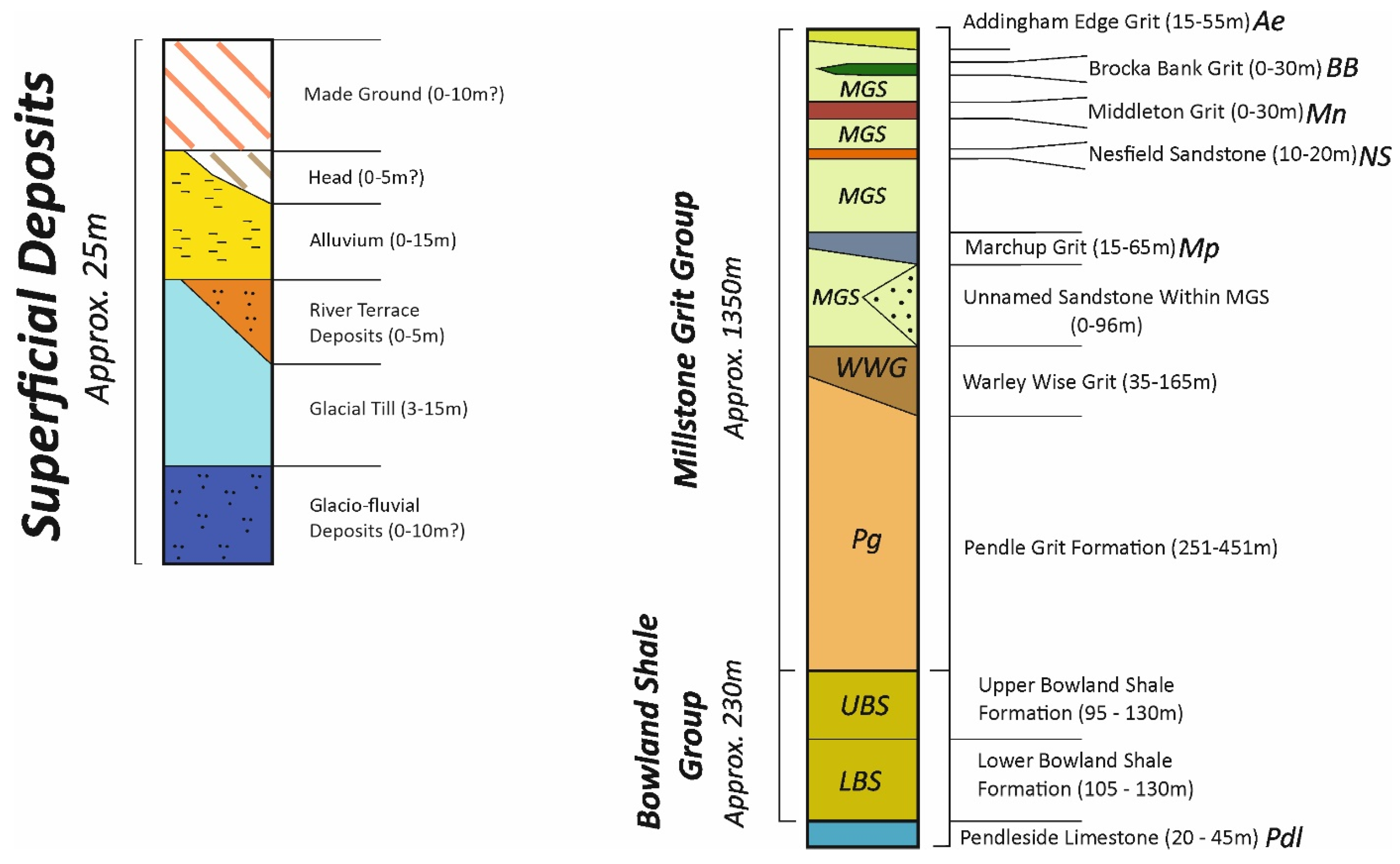
The area has been glaciated, with the last being in the Devensian. Glaciers occupied the lower topographic areas and carved out ‘U’-shaped valleys, leading to formation of elliptical melt out channels up to 50 m thick, corresponding to the current locations of main river catchments [23]. After the Devensian, the current configuration of river catchments was established, and alluvium was deposited. River terrace deposits are also present due to river entrenchment [24]. The generalised stratigraphy of the study area is presented in Figure 4.

Figure 4. Generalised vertical section for the study area, showing thicknesses and major groups. Developed using BGS 1:50,000 sheet 69 map and cross-sections constructed during this study.

Many of the formations are variable in thickness, with the major controls being topographic relief, subsidence, and distance from sediment source. A general description of each of the units is given in Table 1.

Table 1. Engineering geological descriptions for the geology of the study area, using borehole logs, Refs. [23,24].

Geological Unit	Engineering Geological Unit	Description
Made Ground	Anthropogenic Soil	Highly variable, mixture of cohesive and non-cohesive materials
Head	Mixed cohesive and non-cohesive soils	Slipped predominantly cohesive soil (sandy CLAY), poorly consolidated
Alluvium		Mixture of SAND and GRAVEL, SILT and CLAY. High lateral variability, normally consolidated
River Terrace Deposits		Very loose SAND and GRAVEL
Glacial Till		Stiff sandy gravelly CLAY
Glacio-fluvial Deposits		Dense dark grey fine to coarse gravelly COBBLES with finer material (sandy clay)
Addingham Edge grit (Ae)	Moderately strong to strong, medium- to very-coarse-grained SANDSTONE	Medium- to very-coarse-grained, occasionally pebbly, thickly cross-bedded feldspathic SANDSTONE
Brocka Bank Grit (BB)		Fine upward coarsening massive or cross-bedded SANDSTONE
Middleton Grit (Mn)		Medium- to coarse-grained locally pebbly and cross-bedded quartz-felspathic SANDSTONE
Nesfield Sandstone (Ns)		Fine-grained upward coarsening thinly bedded and laminated quartz-arenitic SANDSTONE
Marchup Grit (Mp)		Greyish white medium- to very-coarse-grained cross-bedded SANDSTONE
Warley Wise Grit (WWG)		Very-coarse-grained pebbly cross-bedded SANDSTONE
Pendle Grit (PG)		Medium- to coarse-grained massive felspathic SANDSTONE interbedded with siltstone and very thin mudstone
Millstone Grit Shales (MGS)	Weak to moderately strong MUDSTONE, SILTSTONE, and SHALE	Fissured MUDSTONE, SILTSTONE, and SHALE. Discontinuities are vertical, sub-horizontal, sub-vertical, extremely closely spaced, with some clay infill. Some ironstone concretions and calcite veins
Bowland Shale Group (LBS and UBS)		Fissured calcareous MUDSTONE, SILTSTONE, and SHALE

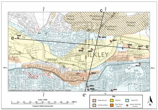
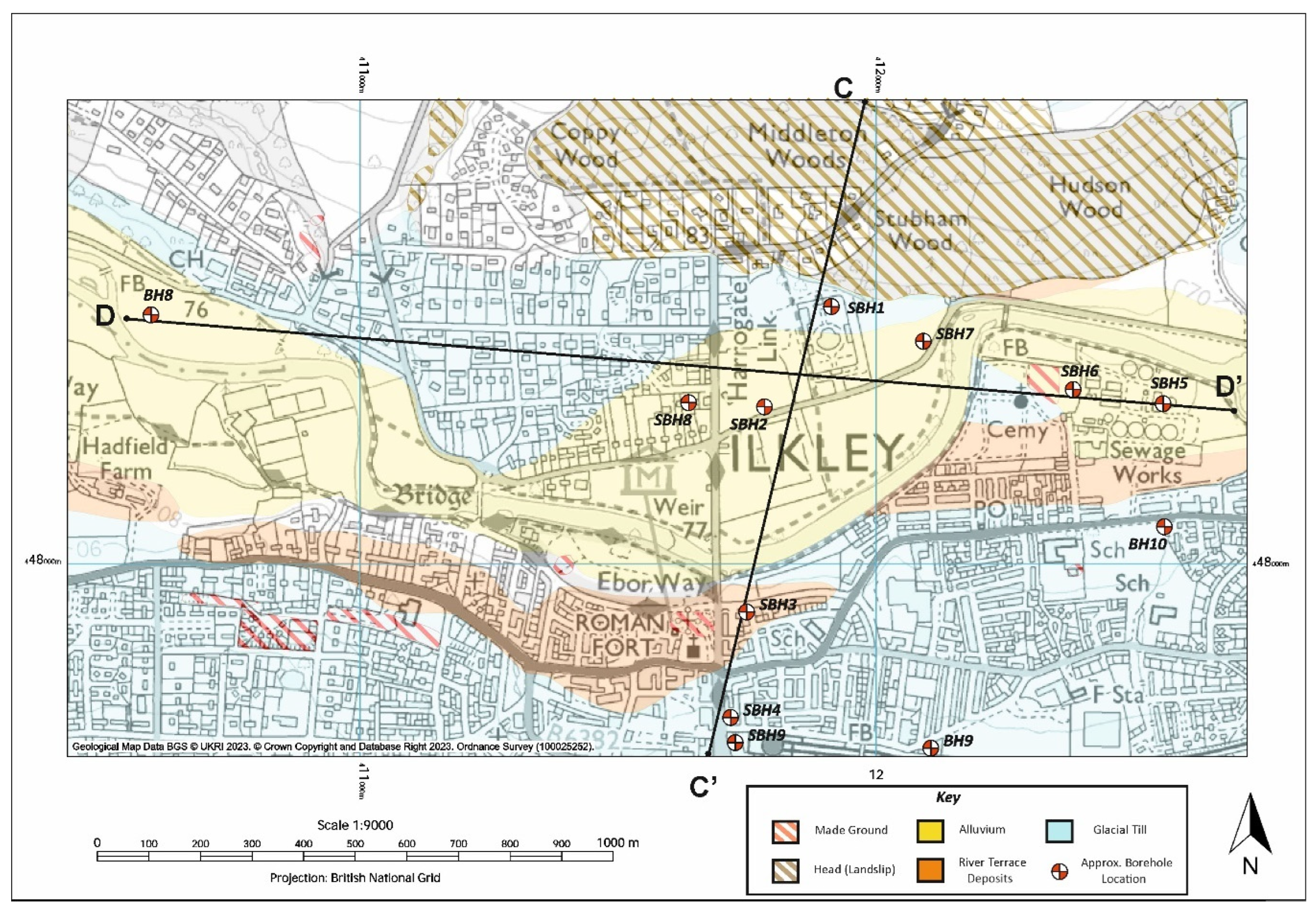
The superficial deposit map for the study area is illustrated in Figure 5, with the borehole locations overlain.

Figure 5. Superficial deposit map for the study area. Ilkley Lido is located roughly at SBH1. Base map downloaded from [10].

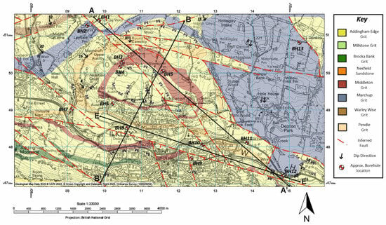
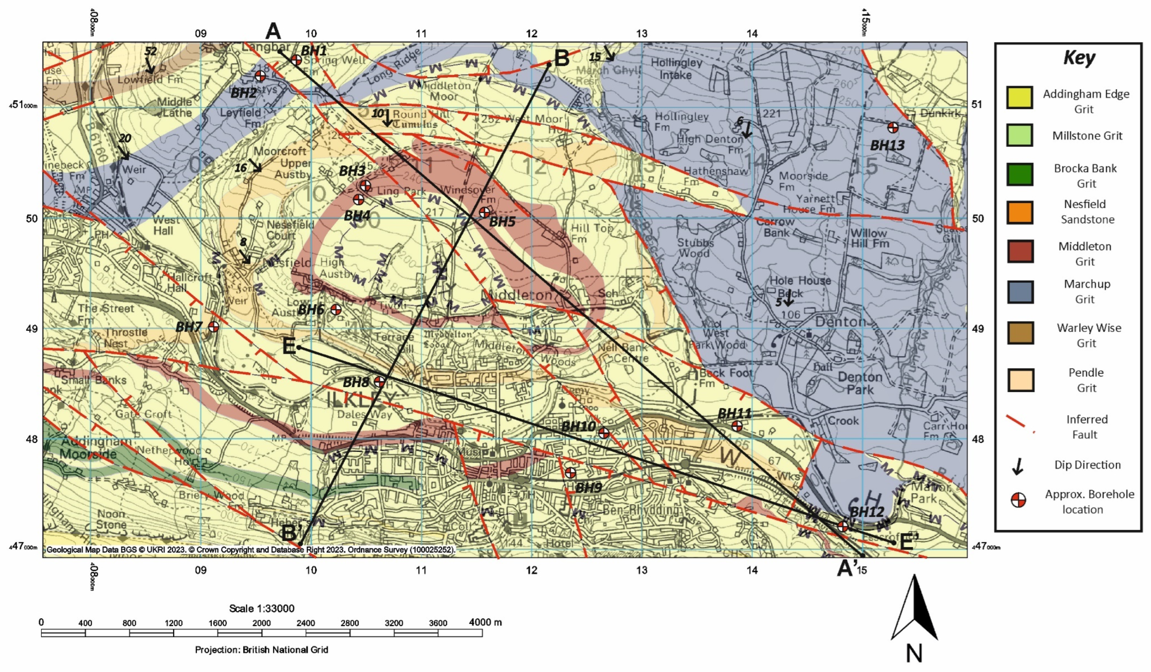
Figure 6 shows the bedrock geology mapping. Outcrop exposure across the region is relatively poor due to vegetation cover and superficial cover. Therefore, the boundaries shown for most faults and geological formations are inferred.

Figure 6. Bedrock geological map of the study area. Base map from [10].

3.2. Geological Structure

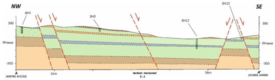
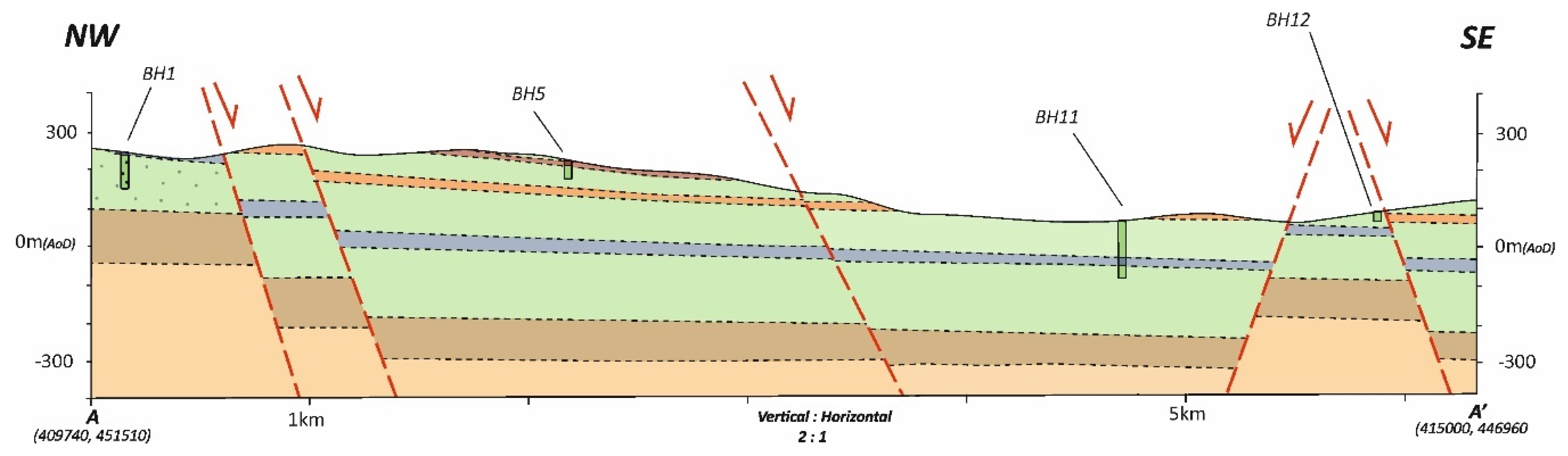
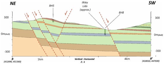
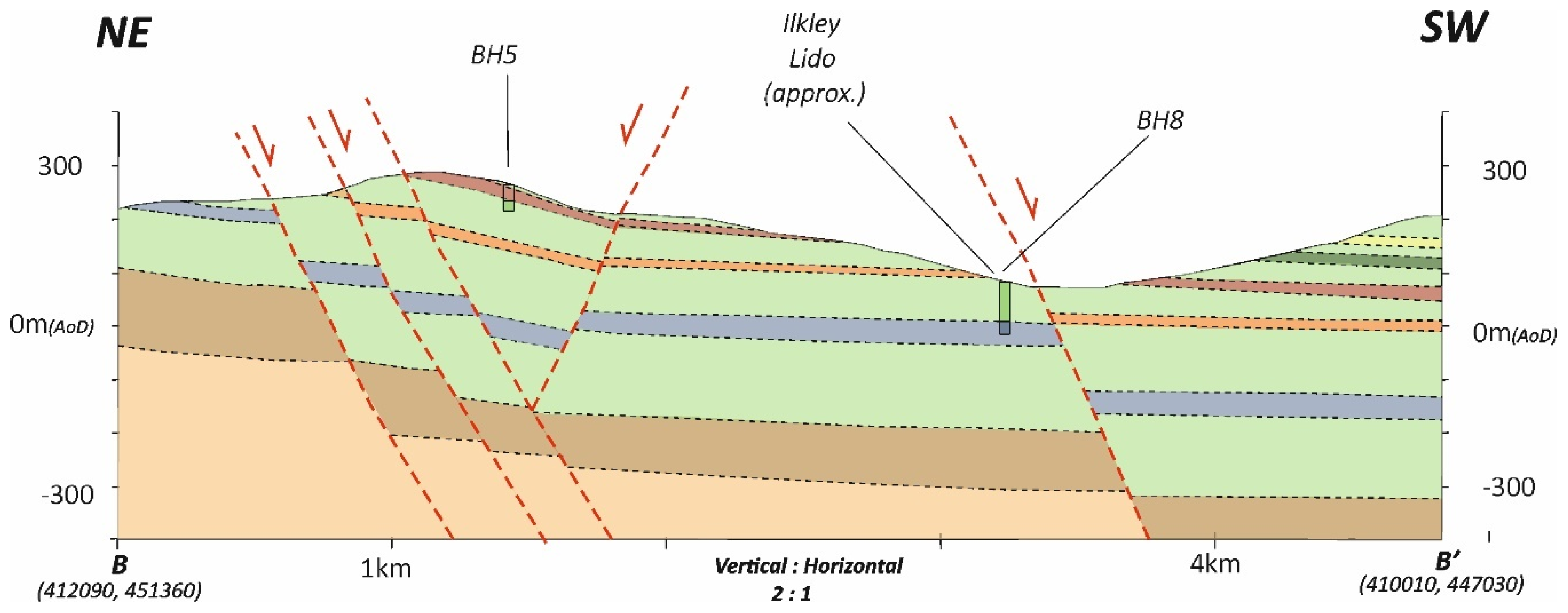
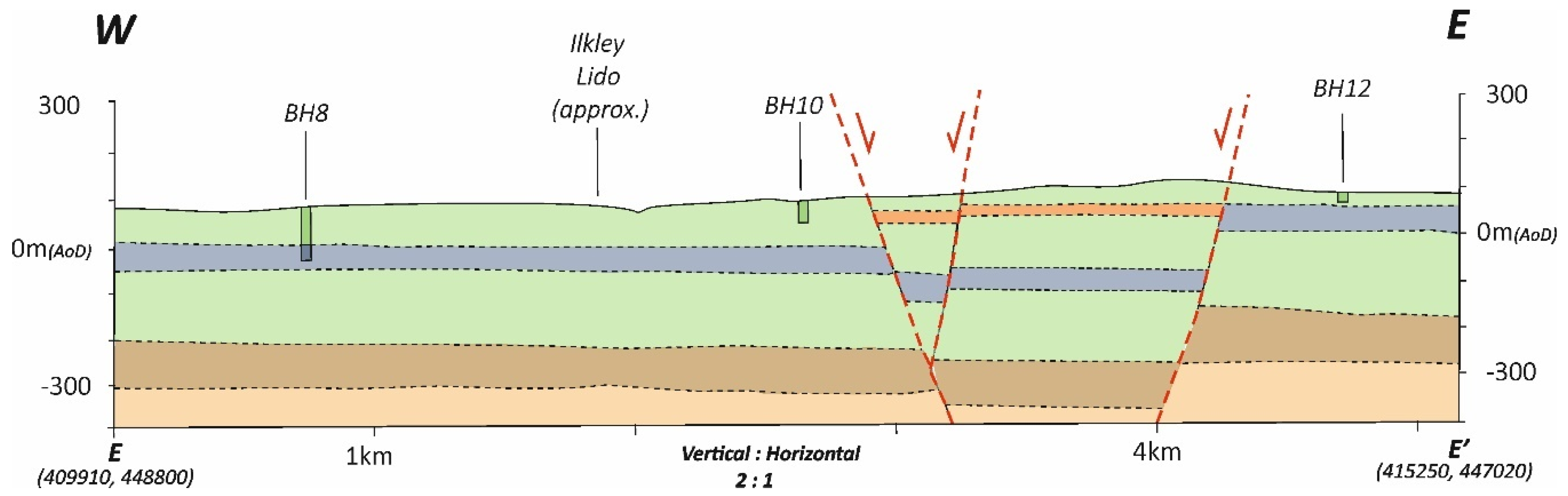
Several geological cross-sections have been produced for this study using all available sources of information and are presented in Figure 7, Figure 8 and Figure 9. Their location and orientation are shown in Figure 6 and Figure 7. Regional dips are between 5° and 10° to the southeast. Namurian strata generally follow the regional trend but can have steeper dips and varying strikes due to faulting [23,24].

Figure 7. Section A-A’, typical horst and graben structures associated with the extensional tectonic regime are prevalent. The MGS in the northwest, around BH1, is an outlier in the study area, comprised predominantly of sandstone, as opposed to shale and mudstone. BH11 fully penetrates Mp and is the nearest borehole with pump test data to the site.

Figure 8. Section B-B’ crosses the faulted block where the study area lies. The beds to the northeast are inferred to be inclined at a greater angle, possibly due to growth faulting. BH8 is the closest borehole to the site and partially penetrates the Marchup Grit (Mp).

Figure 9. Section E-E’ crosses the fault block where the study area lies in the west. An inferred graben structure lies to the east of the site.

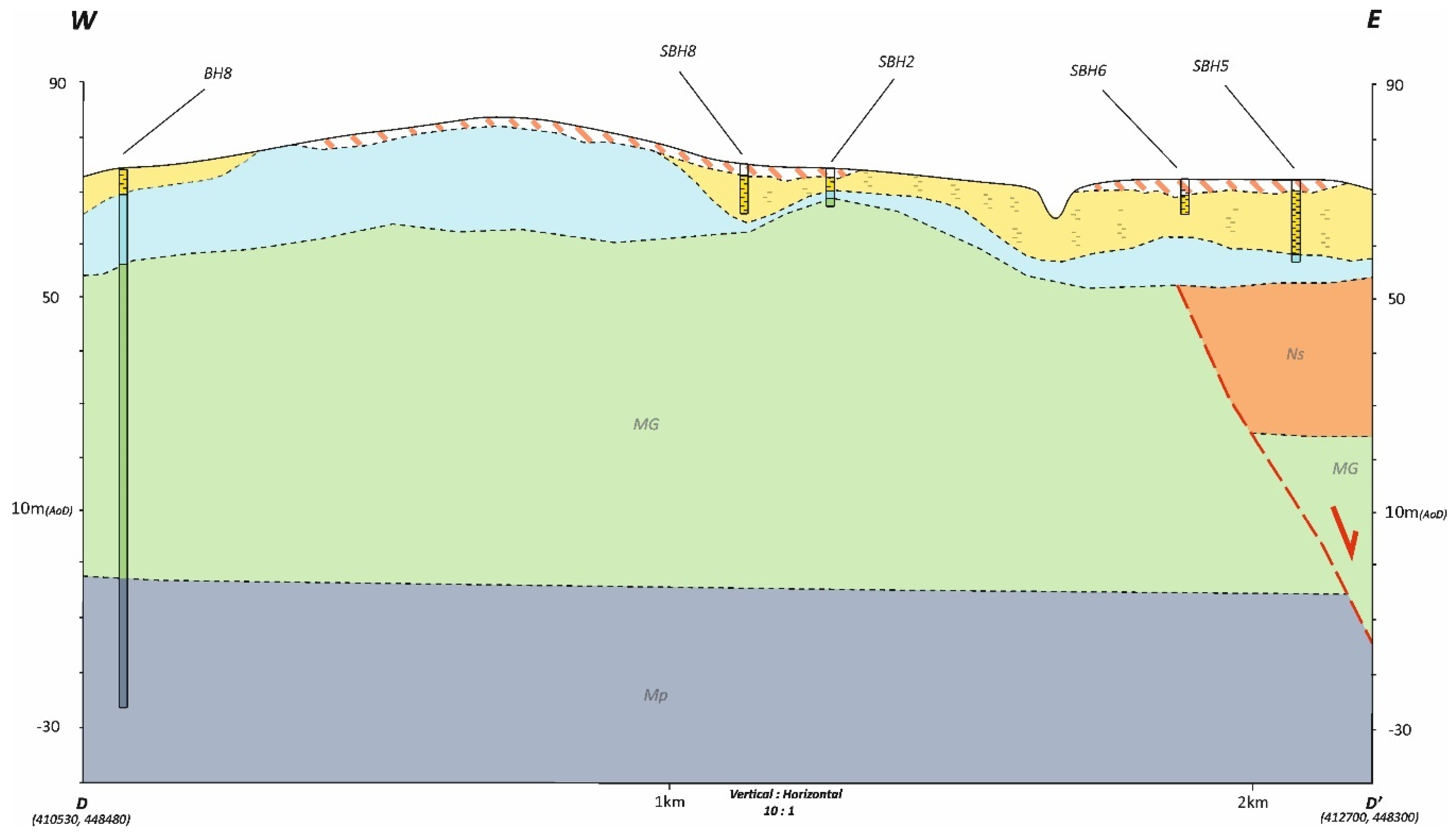
Figure 10 demonstrates the thicknesses of the superficial deposits in the study area and their interactions with the bedrock and faulting below. The cross-section is intended to be illustrative only, as the vertical scale is exaggerated 10:1 to the horizontal scale.

Figure 10. Section D-D’. The variable depth to bedrock is illustrated in this section and inferred between boreholes. A fault is also inferred at this location based on BGS mapping near the site.

3.3. Historic and Current Surrounding Land Use

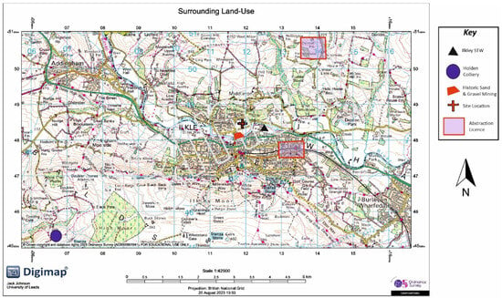
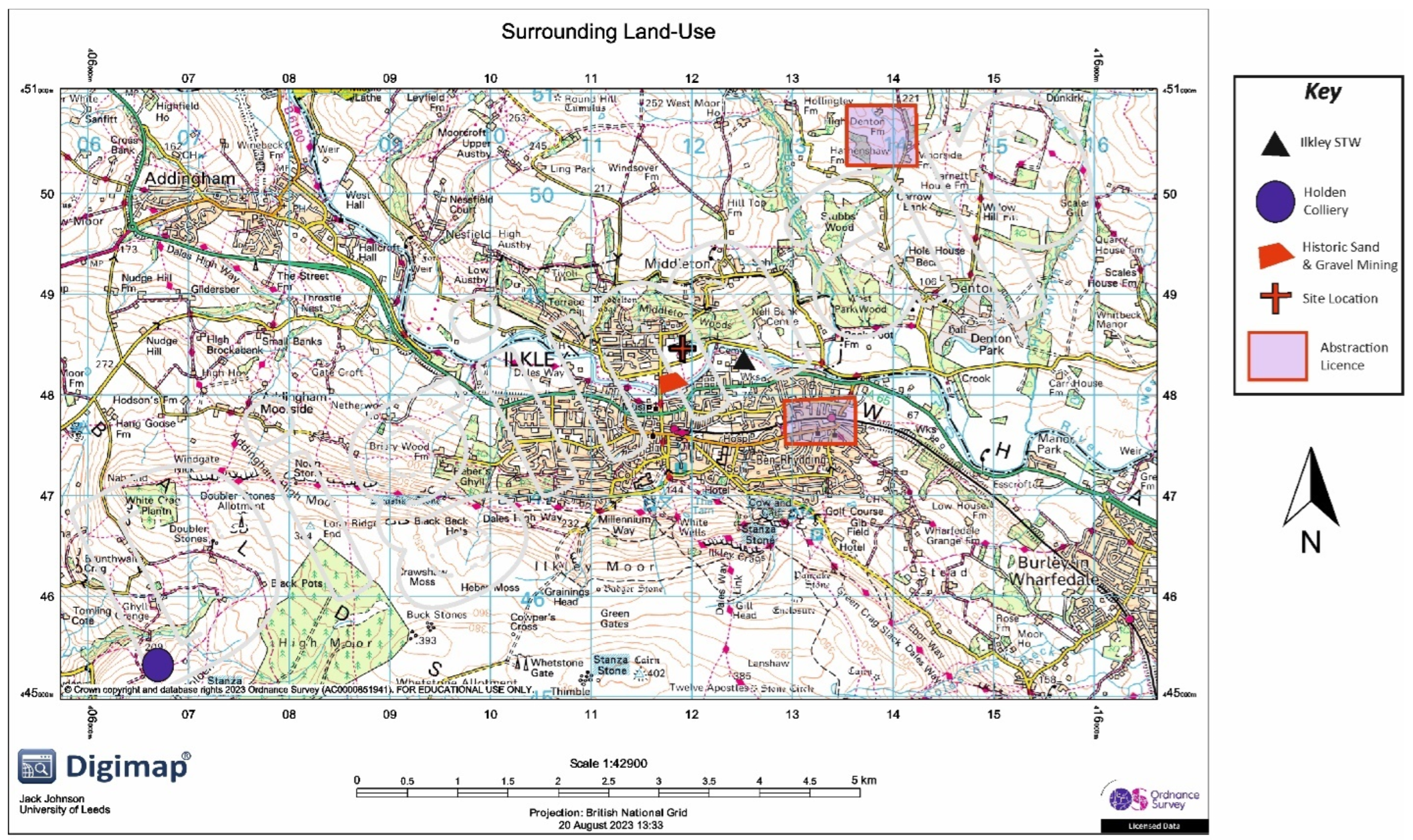
Surrounding land use has the potential to impact groundwater resources in the area; therefore, the historic and current land uses with the largest potential for impacts to a geothermal scheme are assessed. Figure 11 shows the approximate location of the most pertinent surrounding land uses.

Figure 11. Location of Holden Colliery, Ilkley sewage treatment works (STWs), past gravel mining and abstractions in relation to Ilkley Lido and surrounding sports facilities.

The impact of the mining activities is thought to have a negligible impact on the study area, as the regional hydraulic gradient is assumed to be at around 0.01 to the southeast, along the general dip of beds. Therefore, groundwater from Holden Colliery is likely to move to the southeast by the majority and is not likely to reach the study area.

3.4. Hydrogeology

A summary of the available data regarding aquifer properties of the Dinantian Strata and MG group of rocks on a regional basis is given in Table 2. [25] states that the Millstone Grit series of rocks is a multilayered aquifer in which massive sandstone horizons form discrete aquifers, with intervening mudstones and shales. Regionally important aquifers are the WWG and Dinantian Limestones. The data show a wide range in values, which demonstrates the importance of fracture flow in the study area.

Table 2. Aquifer properties from BGS regional studies [26]. Arithmetic mean values in brackets (). Information is from sampling outcrops and BH’s across the Pennine region, with varying amounts of data, from 1 sample to over 100.

Group/Unit Name	Porosity (%)	Storage Coefficient	Specific Capacity (m3/Day)	Hydraulic Conductivity (m/Day)	Transmissivity (m2/Day)	BH Yields (m3/Day)
Dinantian Limestones	1.0–1.3	3 × 10−4	0.35–1900 (91)	-	0.1–1015 (153)	240–1920 (up to 9600 in Malham)
Namurian Sandstones	6–23 (14)	1.3 × 10−2–1 × 10−4	0.54–9092 (140)	3 × 10−4–0.7 (5 × 10−3)	0.6–1059 (93)	432–864 (up to 864)

In addition to the above, nearby historic boreholes with records of pump tests have been processed and are presented in Table 3. The testing was within Mp, but the exact test sections are unknown so are likely to have included contributions to flow from MGS.

Table 3. Mp transmissivity estimates based on BH pump test data.

ID	T (m2 Day−1)	Comments
BH3	20	Partially penetrating Mp
BH4	14	Partially penetrating Mp
BH9	4	Does not penetrate Mp
BH11	11	Fully penetrating Mp, shots fired down the borehole, which is likely to have altered natural transmissivity
BH13	58	Partially penetrates Mp (base assumed to be within 5 m)

Analysis of the pump tests assumes an infinite, non-leaky aquifer pumped from a fully penetrating well, which is not the case for the study area, as the MGS will be contributing to groundwater flow above and below the Mp, and most of the pump tests only partially penetrated the aquifer. In addition, shots were fired in BH11 before the pump test, which is likely to have changed the natural transmissivity.

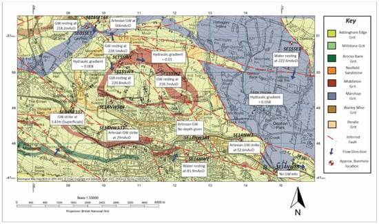
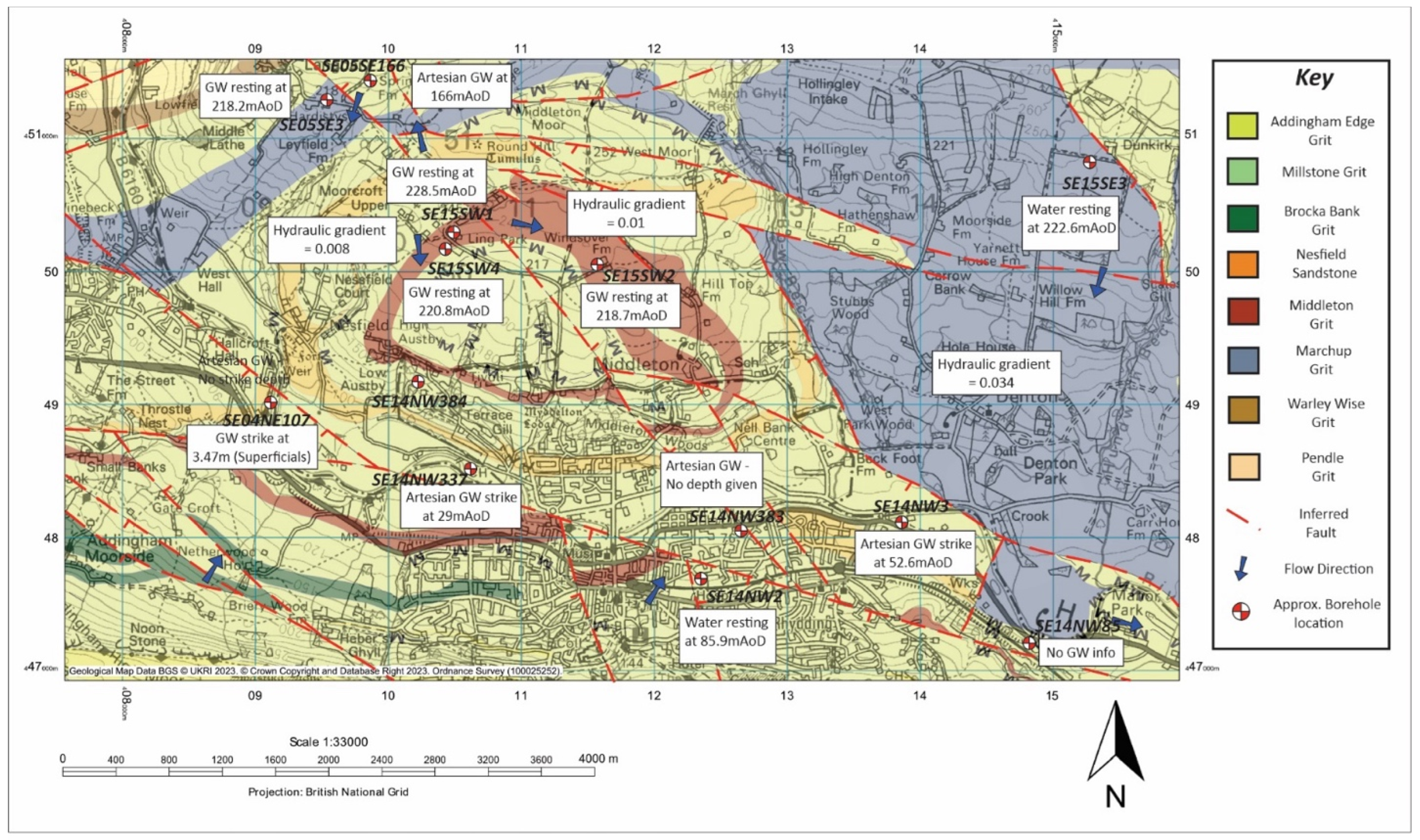
The hydraulic gradient of the confined aquifer comprising Mp with contribution from fracture networks in the MGS is estimated to be between 0.01 and 0.034. The estimate is based on differences in head between several boreholes in the study area, as no hydraulic gradient is available in the literature. Figure 12 shows the estimated flow directions and hydraulic gradients for the study area.

Figure 12. Groundwater flow map showing estimated direction of flow in Marchup Grit based on historic borehole records and topography.

Many of the boreholes do not have groundwater head recorded, only the fact that artesian groundwater was encountered. As the pressure head cannot be correctly determined, these have only been considered qualitatively. The overall direction of flow over the area is assumed to be to the centre of the valley in Ilkley, and generally to the southeast, following the general regional dip of the beds. The same is assumed for the other formations; however, a hydraulic gradient cannot be estimated due to lack of data.

3.5. Groundwater Chemistry

From available chemistry testing, a general decrease in hardness is noted from northwest to southeast (down the general hydraulic gradient), along with an increase in pH, and low levels of nitrate across most tested samples except in BH6. [25] states that the natural baseline in reductive environments within the aquifer is marked by the presence of higher levels of Mn and Fe (>0.5 mg/L and >2.5 mg/L, respectively), and low levels of NO₃-N, which [27] states are indicative of reducing waters.

However, there are still levels of nitrate, and Fe with Mn is not particularly high, so this could be indicative of some groundwater mixing occurring between the layered aquifers, or simply because of mixing of groundwater during drilling of boreholes and sampling.

3.6. Geothermal Properties of Strata in the Study Area

Background heat flow in the UK is fairly uniform at 52 mWm⁻² (disregarding the SW of England), and the average geothermal gradient is 26 °Ckm⁻¹ but can exceed 35 °Ckm⁻¹ locally [9]. Heat flow maps produced by [9] show that the study area lies within a background heat flow area of between 50 and 60 mWm⁻². [6] states that the mean geothermal gradient of Yorkshire’s coalfields, which are immediately to the SE of Ilkley, is 32.3 °Ckm⁻¹. This value should be taken as an upper limit, as the gradient in the coalfields is likely higher than at the study area due to extensive mining causing increased heat from increased groundwater flows and chemical breakdown in mine workings. Table 4 highlights estimates of the thermal properties of strata in the study area.

Table 4. Estimated thermal properties of the main strata in the study area. Thermal conductivity (λ) and volumetric heat capacity (S_vc) are from [12]. Densities are from BH logs. Specific heat capacity (S_c) is calculated by dividing S_vc by density.

Unit	Thermal Conductivity (Wm−1 k−1)	Volumetric Heat Capacity (MJm3 k−1)	Bulk Density (Mg/m3)	Specific Heat Capacity (MJm)
Sandstone	3.75 (±0.16)	2.20 (±0.25)	2.45 (±0.25)	0.90 (±0.25)
Shale	1.80 (±0.16)	2.30 (±0.25)	2.10 (±0.25)	1.10 (±0.25)
Limestone	3.14 (±0.13)	2.40 (±0.25)	2.00 (±0.25)	1.20 (±0.25)

Thermal conductivity variations between massive sandstone beds (λ = 3.75 W/(m*K)) and interbedded mudstones/shales (λ = 1.80 W/(m*K)) establish a highly anisotropic thermal domain. While high-conductivity sandstones facilitate rapid conductive heat extraction during advective flow, low-conductivity shale boundary layers act as insulating caprocks that retard conductive thermal recharge from adjacent strata. Incorporating generic thermophysical constants introduces a +/− 10–15% uncertainty in simulated plume dissipation rates.

4. Fieldwork

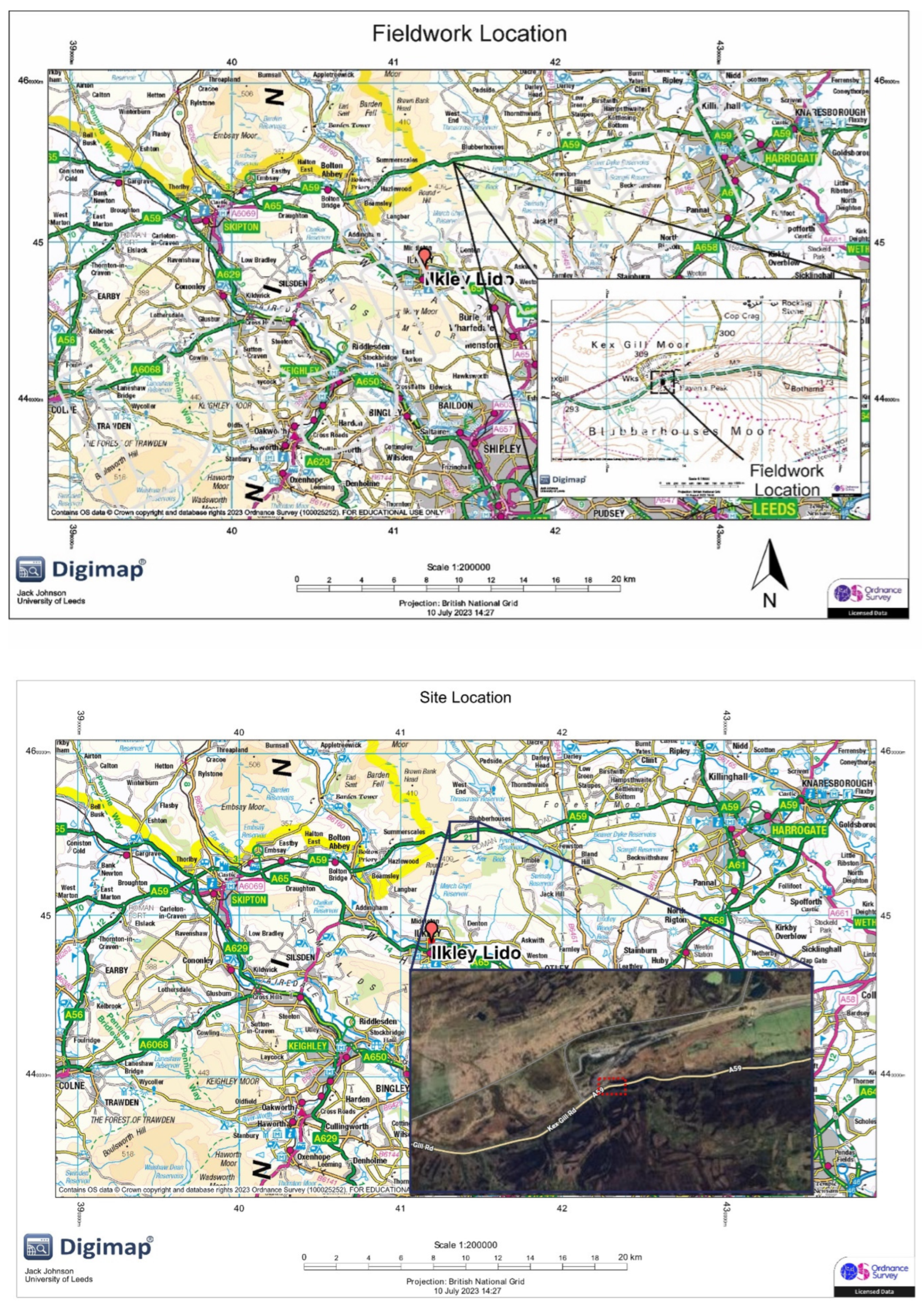
Fieldwork was undertaken on 1 August 2023. The objective of the fieldwork was to obtain information on the target aquifer (Mp). The location of the studied outcrop in relation to the study area is demonstrated in Figure 13.

Figure 13. Location of fieldwork undertaken on 1 August 2023 [10].

4.1. Geological Description of Outcrop

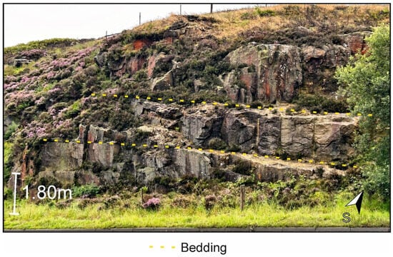
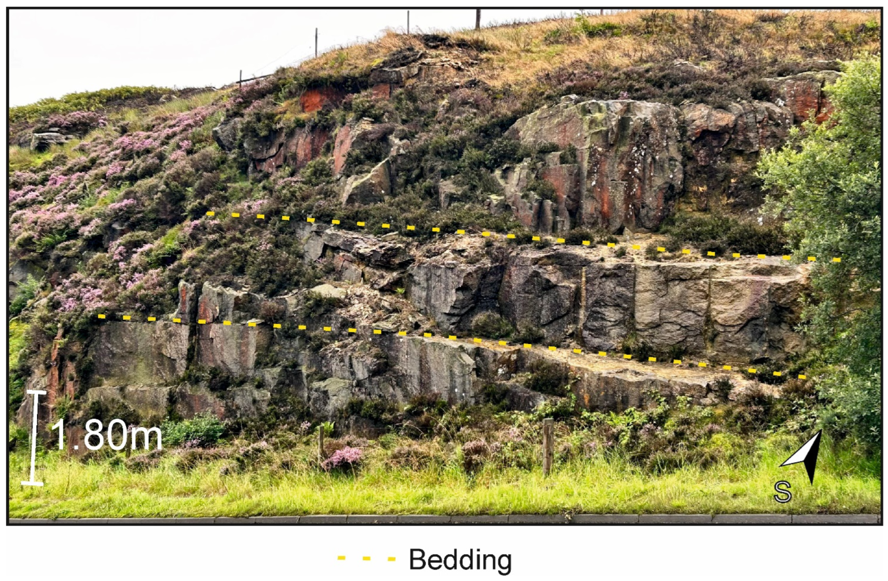
An annotated photo of the studied outcrop is presented in Figure 14. The bedding is outlined by dashed yellow lines. It should be noted that vertical blast marks are present along the rock face and this may have also influenced the condition of discontinuities.

Figure 14. View of the outcrop where data were collected.

Table 5 shows the geological engineering descriptions of the encountered units during fieldwork. Two distinct units were recorded, a strong coarse sandstone (SST1), and a moderately strong, very coarse sandstone (SST2). The main distinction between the two units was the increase in grain size and effects of weathering, with a subangular fine quartz gravel being present in SST2, and SST2 being weathered to sand in places. However, small bands of quartz gravel were also present in SST1. GSI is estimated at between 62 and 68 for the entire rock mass, and the two units are considered representative of Mp.

Table 5. Descriptions of the encountered geology in the field (west of Blubberhouses), recorded from the top of the exposure to the base.

Description	Interpretation	Thickness (m)	Depth to Base (m)
Moderately strong weathered to very weak, thickly bedded to very thickly bedded, greyish white very coarse SANDSTONE with some subangular gravel of quartz. Discoloured orangish brown, decomposed to very coarse sand and fine gravel in places. (SANDSTONE 2 (SST2))	Marchup Grit	1.5	1.5
Strong weathered to very weak, thickly bedded to very thickly bedded, greyish white coarse to very coarse SANDSTONE with occasional inclusions of carbonaceous material up to 2 mm in diameter. Discoloured orangish brown. (SANDSTONE 1 (SST1))	Marchup Grit	1	2.5
Moderately strong weathered to very weak, thickly bedded to very thickly bedded, greyish white very coarse SANDSTONE with much subangular gravel of quartz. Discoloured orangish brown, decomposed to very coarse sand and fine gravel in places. (SST2)	Marchup Grit	3	5.5
Strong weathered to very weak, thickly bedded to very thickly bedded, greyish white coarse to very coarse SANDSTONE with occasional inclusions of carbonaceous material up to 2 mm in diameter and occasional thin bands of quartz gravel. Discoloured orangish brown. (SST1)	Marchup Grit	1.35	6.85

4.2. Discontinuity Surveys

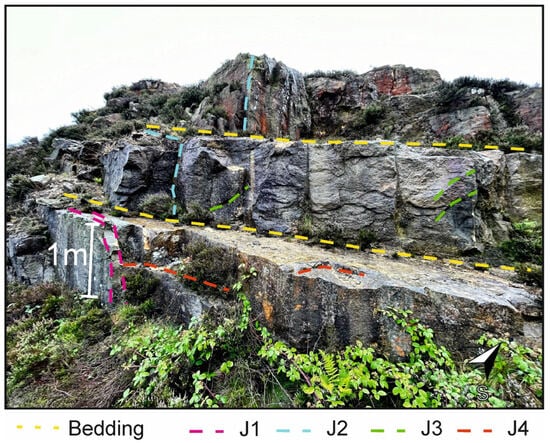
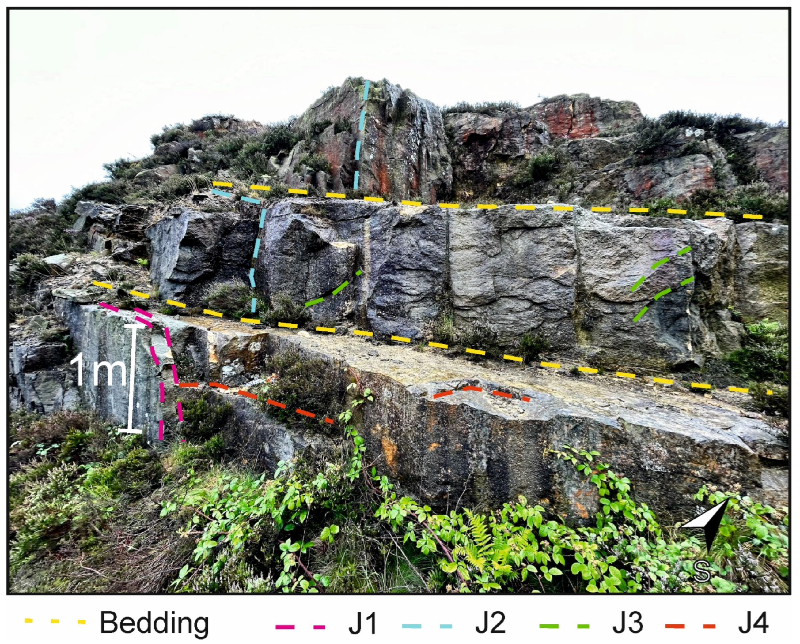
The identified joint sets and bedding in the outcrop are highlighted in Figure 15. The main joint sets are J1 and J2, which are sub-vertical and dip towards ~160° and ~30°, respectively. These joint sets are likely to intersect throughout the formation and have a clayey sand/sand infill in areas. The minor sets (J3 and J4) appear to have a lower persistence and, therefore, are much less likely to intersect.

Figure 15. Closer view of the main section of outcrop, with main discontinuity sets annotated.

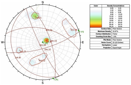
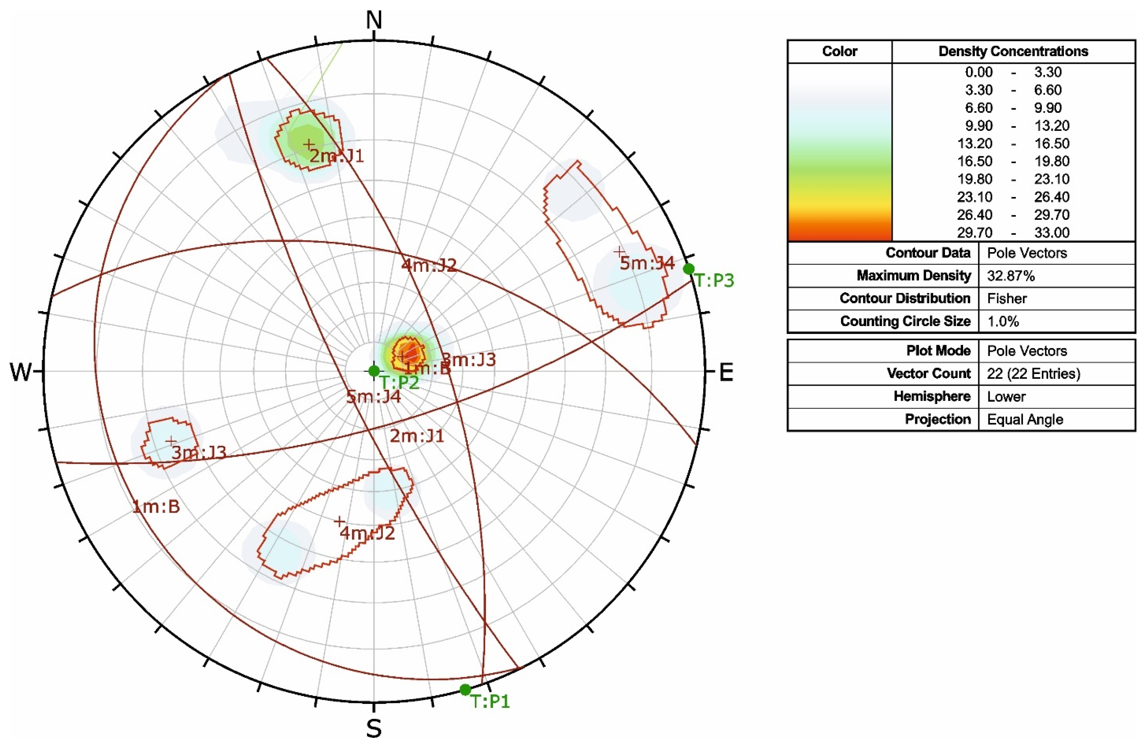
Figure 16 demonstrates that J1 has a higher frequency throughout the outcrop. The dense area near the centre shows the bedding. The other joint sets have a lower frequency.

Figure 16. Stereonet diagram of the discontinuity sets, plotted in Dips (Rocscience^®) using 22 joint measurements. Transects denoted by P1 (into face), P2 (vertical), and P3 (across face).

The mean joint spacing for the Mp was calculated using data from the discontinuity surveys undertaken at the outcrop. These values are presented in Table 6.

Table 6. Calculated mean joint spacing for the Mp, with the x direction being across the face (72–74°), y direction into the face (164–166°), and z vertical.

Mean Spacing in x Plane (m)	Mean Spacing in y Plane (m)	Mean Spacing in z Plane (m)	Average Aperture (mm)
0.62	0.38	0.60	4.8

It should be noted that the Marchup Grit exposure at Kex Gill (Blubberhouses, ~12 km north of Ilkley Lido) provides direct geometric and sedimentological access to the target unit. Although stratigraphically continuous, surface exposures are subject to mechanical weathering and overburden stress relief, which naturally widens aperture dimensions (measured surface mean aperture = 4.8 mm). Consequently, to parameterise the confined subsurface reservoir conservatively, an effective fracture aperture of 1.0 mm and an effective porosity of 10% were adopted for equivalent porous medium-flow calculations.

To bridge the gap between idealised porous media models and the fractured Carboniferous bedrock, field discontinuity surveys (joint sets J1 and J2) and microscopic pore thresholding were synthesised into weighted permeability tensors (Equation (11), see Section 4.4). This equivalent continuous porous medium (ECPM) approach adapts standard continuum calculations to fractured sandstone conditions by explicitly incorporating both primary matrix permeability and secondary fracture transmissivity.

4.3. Porosity Estimates

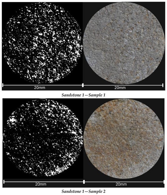
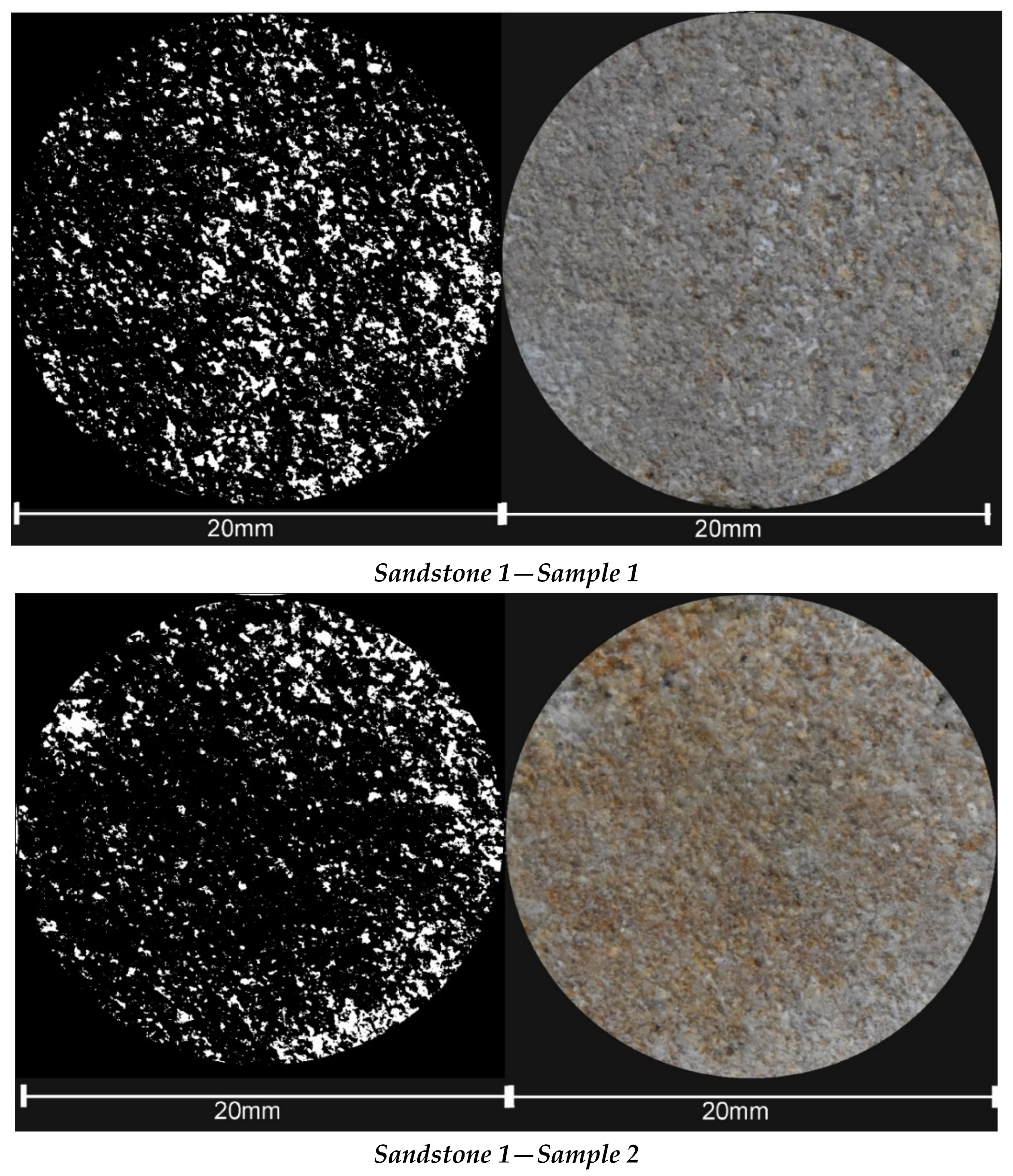
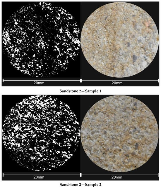
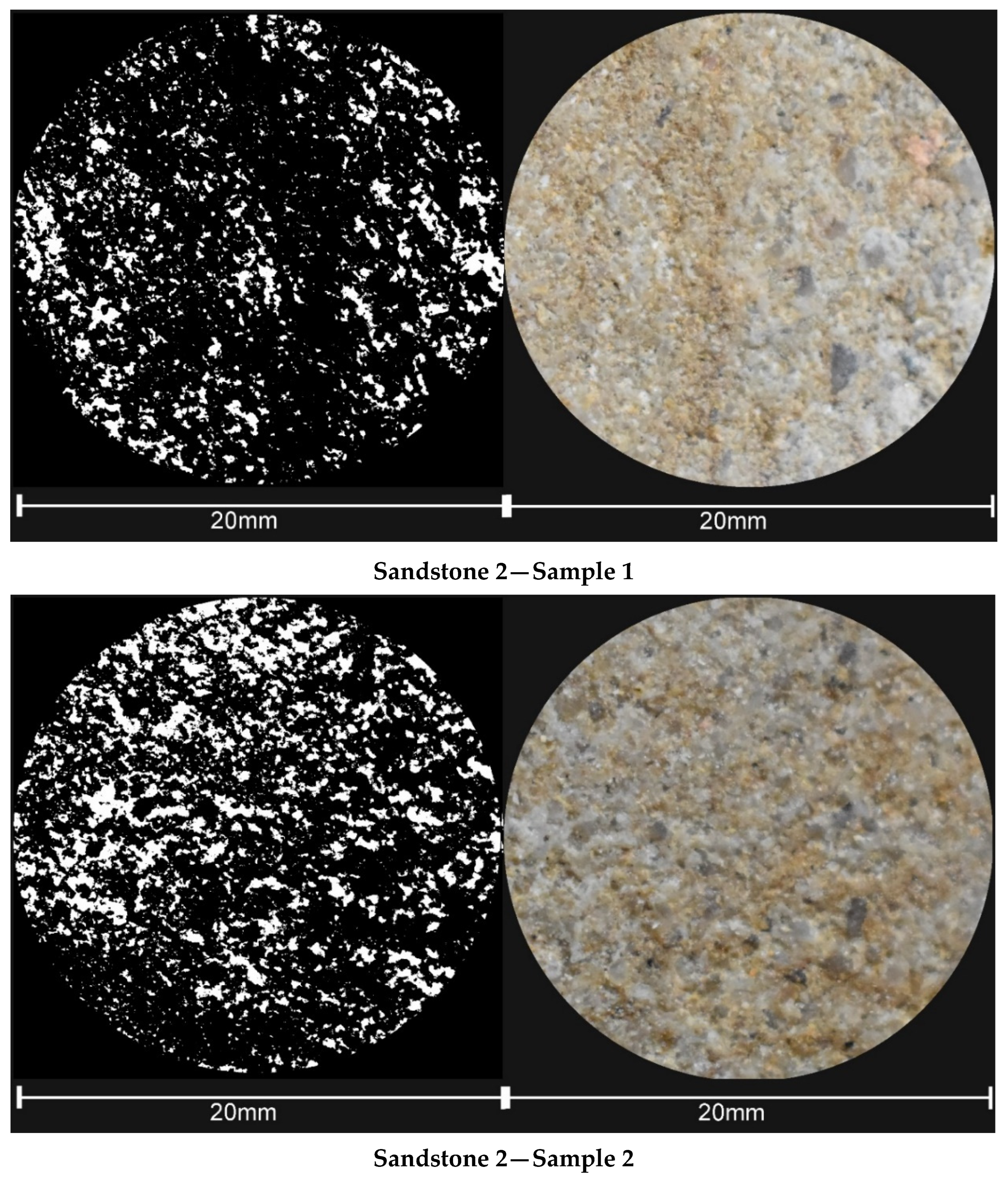
Images of hand samples taken from the outcrop were analysed to estimate the porosity of Mp and are displayed in Figure 17 and Figure 18. The images were analysed using the auto-threshold function in ImageJ to reduce bias; however, this cannot be eliminated, as ultimately selection of an appropriate image is still required. The samples were prepared by sawing the faces vertically.

Figure 17. Hand sample photos of Sandstone 1. Taken using a Nikon D3500 24 Megapixel camera. Image on the left was processed using ImageJ and the auto-threshold function.

Figure 18. Hand sample photos of Sandstone 2. Taken using a Nikon D3500 24 Megapixel camera. Image on the left was processed using ImageJ and the auto-threshold function.

A porosity can be calculated from the image with a threshold applied to the measured pixel area of the image, which corresponds to pore space in the rock. Table 7 shows the estimated values from the four hand samples. The values are suitable as estimates and fit within the regional values for Namurian Sandstones. A mean porosity for both units is reported, as this is more applicable to the formation based on expected values and limitations with the data along with processing techniques.

Table 7. Estimated porosity values from processed hand sample images.

Sample Number	Estimated Porosity (%)	Mean Porosity (%)
SST1—S1	12.8	13.8
SST1—S2	10.3
SST2—S1	12.7
SST2—S2	19.2

4.4. Fracture and Matrix Permeability

Using the estimates of porosity and fracture spacing, an estimate of fracture permeability within the Mp has been made. The RPGZ model [28] was used to calculate matrix permeability using Equation (8):

$$K_h = {\displaystyle \frac{d^2{\phi }^{3m}}{4\alpha m^2}},$$

(8)

where K is horizontal matrix permeability in m², d is the mean grain size, φ is porosity, m is the cementation exponent (assumed as 2), and α is equal to 8/3.

Estimation of vertical matrix permeability can be made using Equation (9):

$$K_v = {\displaystyle \frac{K_h}{3}},$$

(9)

and fracture permeability can be estimated from Equation (10) [18]:

$$K_f = {\displaystyle \frac{b^3}{12s}},$$

(10)

where b is fracture aperture, and s is the mean fracture spacing.

A weighted arithmetic mean value for horizontal permeability can then be calculated using Equation (11):

$$K_{\mathit{hm}} = {\displaystyle \frac{{(k}_f \times b) + {(k}_h\times s)}{(b + s)}}.$$

(11)

The equations above were used to calculate an average horizontal permeability for Mp. Table 8 shows the estimated values calculated with discontinuity and matrix porosity data estimated from fieldwork data.

Table 8. Estimates of hydraulic conductivity of Mp, based on average values taken from fieldwork data.

Φ (%)	kh (m/Day)	Kv (m/Day)	Kf (m/Day)	khm (m/Day)	kvm (m/Day)
10	3.2 × 10−15	1 × 10−15	5.2 × 10−12	1.2 × 10−3	4 × 10−4

A lower porosity of 10% was used in the calculations to represent the effective porosity, and calculations were made using average joint spacing of 0.6 m and an aperture of 1 mm to provide conservative estimates of permeability, as apertures are likely to close with increased overburden pressure. The estimate of k_hm fits within the quoted range in the literature for hydraulic conductivity of Namurian sandstones.

To bridge the gap between idealised porous media models and the fractured Carboniferous bedrock, field discontinuity surveys (joint sets J1 and J2) and microscopic pore thresholding were synthesised into weighted permeability tensors (Equation (11)). This equivalent continuous porous medium (ECPM) approach adapts standard continuum calculations to fractured sandstone conditions by explicitly incorporating both primary matrix permeability and secondary fracture transmissivity. While this continuum representation captures the bulk hydrodynamic transmission of the formation under regional gradients, localised preferential flow along individual dilated fracture corridors cannot be fully resolved at this scale.

4.5. Schmidt Hammer Testing

Four Schmidt hammer tests were undertaken to provide estimates of unconfined compressive strength (UCS). The mean rebound values taken from 20 measurements at each test location and the estimated UCS value are both reported in Table 9 below.

Table 9. Estimates of UCS from Schmidt hammer data. Assuming a bulk density of 2450 kg/m³.

	Test 1 (SST1)	Test 2 (SST1)	Test 3 (SST2)	Test 4 (SST2)
Mean ‘R’ Value	41	44.5	26.5	19
UCS (MPa)	70	90	52	21
Mean UCS (MPa)	80		36.5

There is a clear difference between the values, with the mean UCS of SST1 being over double the UCS of SST2. This demonstrates either anisotropy between the beds or heterogeneity between the lateral extents of the beds, which could be because of weathering.

5. Heat Demand

Gas and electricity usage was supplied by Ilkley Rugby Club, and Table 10 shows the heating and cooling demand of the building based on the usage.

Table 10. Heating and cooling demand of Ilkley Rugby Club, based on usage data kindly supplied by the Rugby Club. Assumed 12 h of operation per day for cooling and heating.

	Usage (kWh)	Usage per Day (kWh)	Usage per Day (kW)
Annual Electricity Usage	42,570			Cooling Demand
Peak Electricity Usage		160	13.5
Mean Electricity Usage		68	5.6
Annual Gas Usage	109,860			Heating Demand
Peak Gas Usage		460	38.5
Mean Gas Usage		300	25

The baseline thermal load is derived from metred gas and electrical records supplied by Ilkley Rugby Club, operating on an operational profile of 12 h/day. To estimate the combined load of the Ilkley Lido complex, a geometric scaling factor of 1.7 was applied, matching the total heated footprint (1460 m² vs. 860 m²) shown in Table 11. Heating demand strongly dominates the site profile across autumn, winter, and spring. While space cooling demands are minimal for municipal Lido halls under UK climatic conditions, a theoretical cooling load (assuming 50% summer HVAC electrical split) is modelled to assess bidirectional thermal regeneration of the aquifer.

Table 11. Estimates for Ilkley Lido buildings’ heating and cooling demand.

	Peak (kW)	Mean (kW)
Heating Demand	65.4	42.4
Cooling Demand	22.9	9.5

The estimate assumes that the buildings are constructed of similar materials, that the usage is similar and over the same time, and that the buildings are insulated to the same standards.

6. Feasibility Study

6.1. Conceptual Ground Model

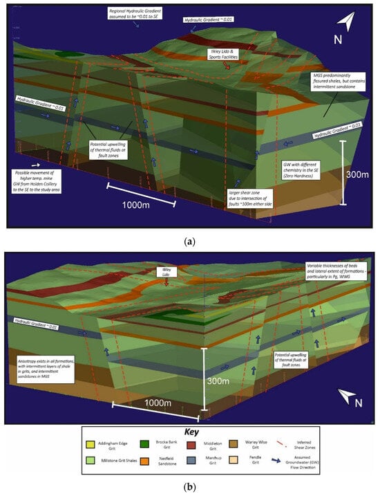
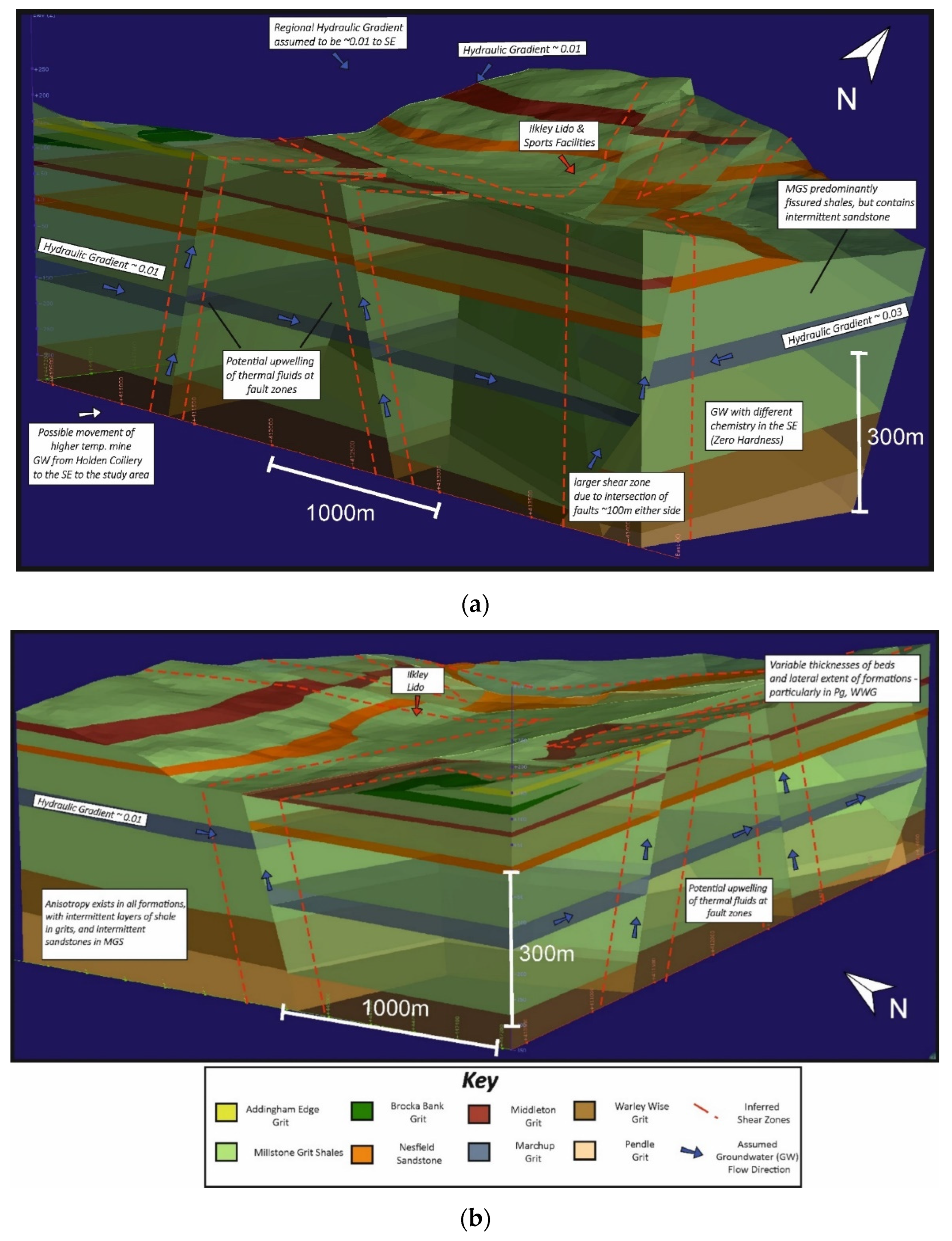
This section outlines the conceptual ground model for the study area, which was constructed from all available data. A representative 3D model of the geology of the area is outlined in Figure 19.

Figure 19. Conceptual geological model produced in Leapfrog Geo software. The model illustrates the likely 3D architecture of the area surrounding Ilkley Lido. (a) A view of the model facing northwest. A large shear zone is noted to the southeast of the site and highlighted in the model. A historic colliery is located within approximately 5 km and may contribute higher-temperature water to the area. (b) A view of the conceptual model facing northeast with Ilkley Lido around the centre. The variable thicknesses of beds are not adequately expressed due to scale and distal data points.

Flow lines denote the approximate flow direction, and parameters are superimposed on the figure. Fault shear zones can act as a conduit for fluid flow and are marked on the image. However, faulted zones can also have the opposite effect, where aquitards of the MGS are brought into contact with the formations that comprise aquifers.

The fracture zones are assumed to be at least ~100 m either side of faults due to evidence of significant fracturing in BH12, which is recorded at ~100 m from faults in the southeast. The discontinuities recorded in this log are sub-vertical, vertical, sub-horizontal, and horizontal, with rock core recorded as non-intact and having zero rock quality designation values. Although the borehole represents a very small area it can be used to broadly state that the fracturing within the MGS is extensive, at least around the shear zones, and this will have a positive effect on expected flows in those areas overall. Numerous calcite veins are also recorded, which according to [29] are more numerous, with increased levels of cooling of hydrothermal fluids at distal areas to upflow zones along faults.

Groundwater chemistry is variable between harder waters in the northeast of the study area, and very soft water in the southeast. Available information suggests that the hardness of the water at the site is likely to decrease down gradient, and the expected level of hardness is <100 mg/L. However, groundwater conditions are not static, especially where wells are introduced into an aquifer. There is a risk of increasing hardness over time if zones of calcite alteration (which are confirmed to the southeast) are affected by changing gradients and head, which could dissolve the calcite and bring it to the abstraction well in solution.

Methane and other gases, such as hydrogen sulphide, could potentially be present at depth based on comments of sulphur odours from wells on nearby BH logs (BH11) and due to the nature of the underlying Bowland Shales Group. However, Ref. [30] shows that groundwater flow can retain significant amounts of ground gas, specifically methane at depth, so there could be a relatively low risk if GW levels and gradients are maintained.

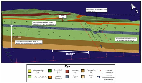
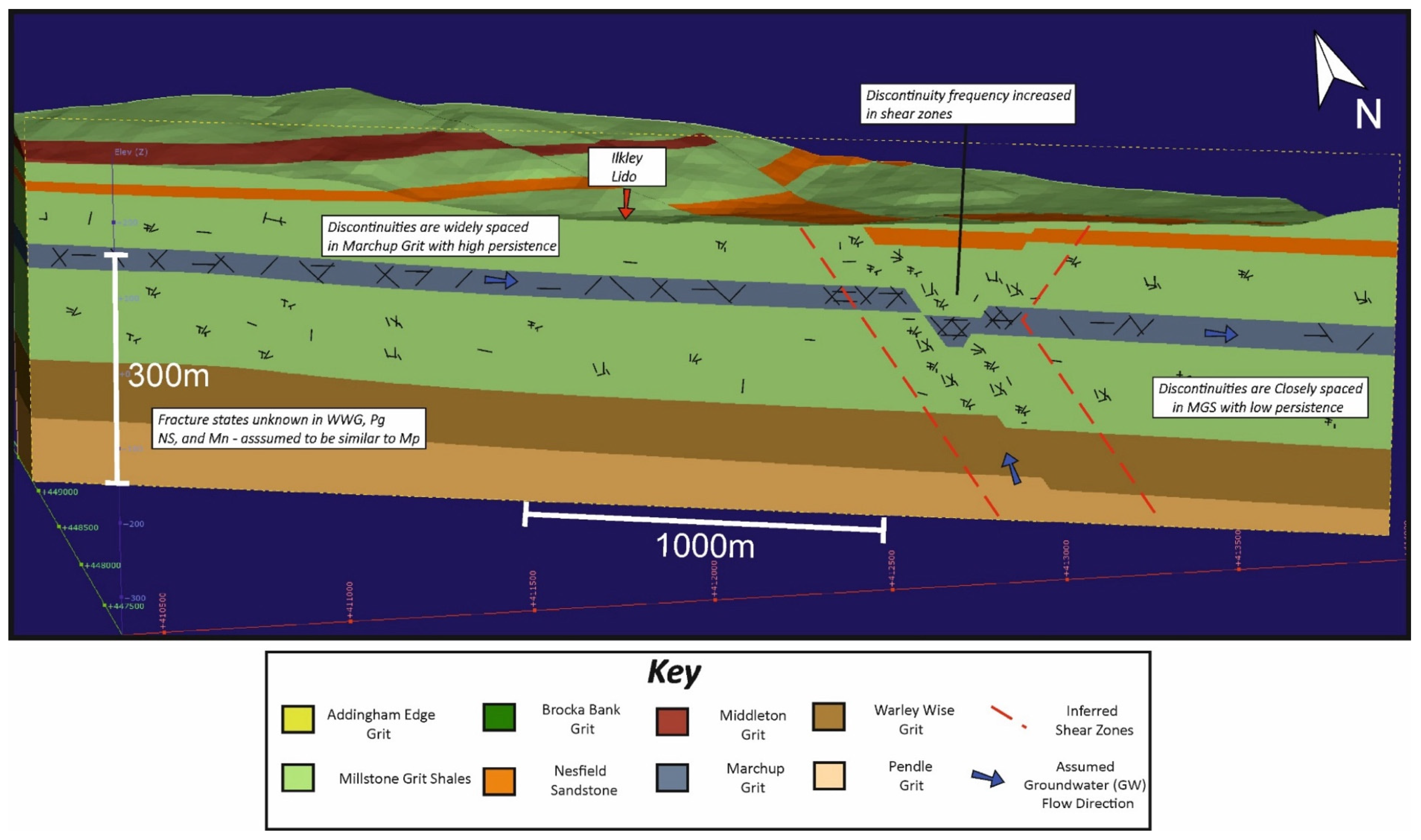
Fieldwork identified four major planes of discontinuities in Mp, with both being near-vertical joint sets, and two sub-vertical sets. These fractures are illustrated in Figure 20 and will affect the vertical and horizontal permeability of the formation, which will also be affected by the variability in characteristics of the two units that make up this aquifer.

Figure 20. Conceptual model looking NE. Annotated surface is a slice through the model orientated NW to SE.

The other major consideration of the ground model is the fact that the formations all have some degree of anisotropy, with the grits having variable amounts of interbedded shales and marine bands, and the MGS having some intermittent sandstones. Each of these units will have negative and positive contributions to flow in each respective formation.

Superficial deposits are omitted from the model. However, the cross-section shown in Figure 10 demonstrates the expected superficial geology. Alluvium and glacial till are recorded in boreholes, and potentially glacio-fluvial deposits near the River Wharfe. The presence of glacio-fluvial deposits is likely but cannot be confirmed due to lack of data. These are likely the most suitable superficial deposits for GSHP systems due to the potential for high porosity and groundwater flows.

6.2. Geothermal Gradient

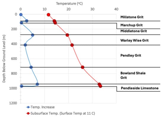
Using the conceptual geothermal model, and thermal properties given in the literature, an assessment of the geothermal gradient has been made for the study area. Table 12 shows the calculated values for the geothermal gradient and the expected temperatures at depth. Uncertainty increases with depth due to the lack of data regarding the depth of strata below the base of boreholes (maximum depth is 152 m in BH11), and all thermal properties are estimated due to lack of site-specific data.

Table 12. Estimated geothermal gradients and subsurface temperatures based on available data for each formation. Uncertainties are estimated based upon the reliability and applicability of the data to the assumed ground conditions and depths. Data are estimated from cross-sections, geological models, and regional data in the BGS Bradford sheet 69 1:50,000 mapping, along with [9,12,23].

Strata	Depth to Base (mbgl)	Thermal Conductivity (Wm−1K−1)	Geothermal Gradient (Km−1)	Subsurface Temperature (°C)
Alluvium	5 (±0.5)	1.7 (±0.3)	0.032 (±0.005)	11.7 (±1)
Millstone Grit	90 (±1)	1.8 (±0.3)	0.031 (±0.005)	14.1 (±0.5)
Marchup Grit	115 (±5)	3.75 (±0.16)	0.015 (±0.005)	14.5 (±0.5)
Millstone Grit	280 (±10)	1.8 (±0.3)	0.031 (±0.005)	19.5 (±1)
Warley Wise Grit	415 (±20)	3.75 (±0.16)	0.015 (±0.005)	21.5 (±1)
Pendle Grit	715 (±100)	3.75 (±0.16)	0.015 (±0.010)	25.9 (±2)
Bowland Shale	945 (±100)	1.8 (±0.3)	0.031 (±0.010)	32.9 (±2)
Pendleside Limestone	970 (±100)	3.14 (±0.13)	0.018 (±0.010)	33.4 (±2)

The graph in Figure 21 demonstrates that the highest increases in temperature are in the formations predominantly comprised of shales and mudstones. This results in higher expected temperatures in the more permeable underlying formations of Mp, WWG, and Pdl. The mean geothermal gradient for the strata at ground level to the base of Mp is 0.026 °Cm⁻¹.

Figure 21. Temperature variation with depth directly below the study area. Data are derived from geothermal gradient calculations in Table 12.

6.3. Estimated Flow Rates to Meet Heat Demand

Using the values in the literature presented in Section 3 and calculated values in Section 4, entered into Equations (2) and (3), flow rates can be estimated to match the example heat demand for Ilkley Lido. Table 13 shows the estimated flow rates required by assuming typical parameters for a heat pump with a COP of 4, and assuming a refrigerant with a typical boiling point of 7 °C is used.

Table 13. Estimated flow rates to meet heating and cooling demand for Ilkley Lido, within strata to approximately 1 km below ground level. Rounded to the nearest 5 m³day⁻¹.

Strata	Mean Cooling Flow Rate (m3day−1)	Peak Cooling Flow Rate (m3day−1)	Mean Heating Flow Rate (m3day−1)	Peak Heating Flow Rate (m3day−1)
Alluvium	55	130	140	220
Millstone Grit	35	85	95	140
March Up Grit	35	80	90	135
Millstone Grit	20	50	55	80
Warley Wise Grit	20	40	45	70
Pendle Grit	15	30	35	55

Based upon these estimates, shallow aquifers within the superficial deposits are not deemed to be feasible for open-loop systems beneath the study area, as the required flow rates are likely to be unachievable on a short- or long-term basis. The same can be said for the Millstone Grit Shale, which is unlikely to yield significant groundwater flows due to being comprised of low-transmissivity shales and mudstones.

The flow rates within Mp could be feasible, with nearby boreholes yielding 432 m³/day, as discussed in Section 4.5, and a nearby pump test undertaken in the same geological section (BH11) recorded average yields of 190 m³/day over 12 days. The WWG and PG could also be considered but the Mp is at a shallower depth and is likely to yield the required amounts of groundwater. The expected flow rate to meet peak heating demand for the Rugby Club and Lido would be approximately 220 m³/day, which is slightly higher than the nearby yields, but it should be noted that at the end of the pump tests the wells were still presenting artesian conditions.

6.4. Expected Drawdown

Drawdowns within the wells can be approximated based on transmissivity and pumping rates [31]. The expected drawdown should be at least ten metres above the top of an abstraction within confined aquifers to prevent clogging and precipitation of minerals within the aquifer, which can progressively deteriorate the quality and rates of groundwater achievable [12]. Equation (12) was used to estimate drawdowns using transmissivity values from pump test data:

$$S_{w }= {\displaystyle \frac{2Z}{T}}.$$

(12)

Table 14 shows the expected drawdowns based on this equation for the different flow rates and range of transmissivities. The base of the Mp is assumed to be around 88 m below the ground level of the Lido. Therefore, drawdowns will reach the top of the aquifer if an abstraction of 220 m³/day is pursued, and transmissivities are ~5 m²/day or less.

Table 14. Range of drawdowns based on lowest and mean values of T in the study area.

Source	T (m2day−1)	Pump Rate (m3day−1)	Sw (m)
Lowest T from pump tests	4	220	110
		135	68
Mean T from pump tests	25.8	220	17
		135	11

6.5. Well Spacing

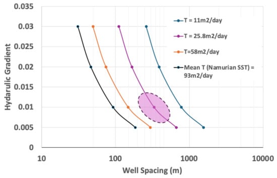
Using the equations outlined in Section 2.2, an estimate of optimal well spacing can be made. Optimal well spacing is a spacing that results in negligible or no hydraulic and thermal feedback from the injection well to the abstraction well. Using conservative values as an upper and lower range, the optimal well spacing based on hydraulic feedback is outlined as the shaded area in Figure 22 and corresponds to between 290 m and 940 m. The mean transmissivity, as reported by [26], is the black line on the plot, to give context.

Figure 22. Plot of well spacing against the hydraulic gradient, with transmissivities of aquifers from pump test data in Section 4.5. The hydraulic gradient is varied to fit the range of expected values.

The available space at Ilkley Lido restricts the spacing of the wells to a more realistic range of approximately 130 m to 350 m; therefore, some degree of hydraulic feedback, and subsequently thermal feedback, is inevitable depending on the final well layout and actual ground conditions.

6.6. Hydraulic and Thermal Feedback Results

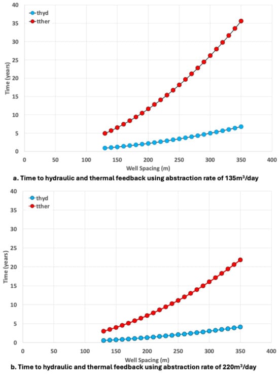
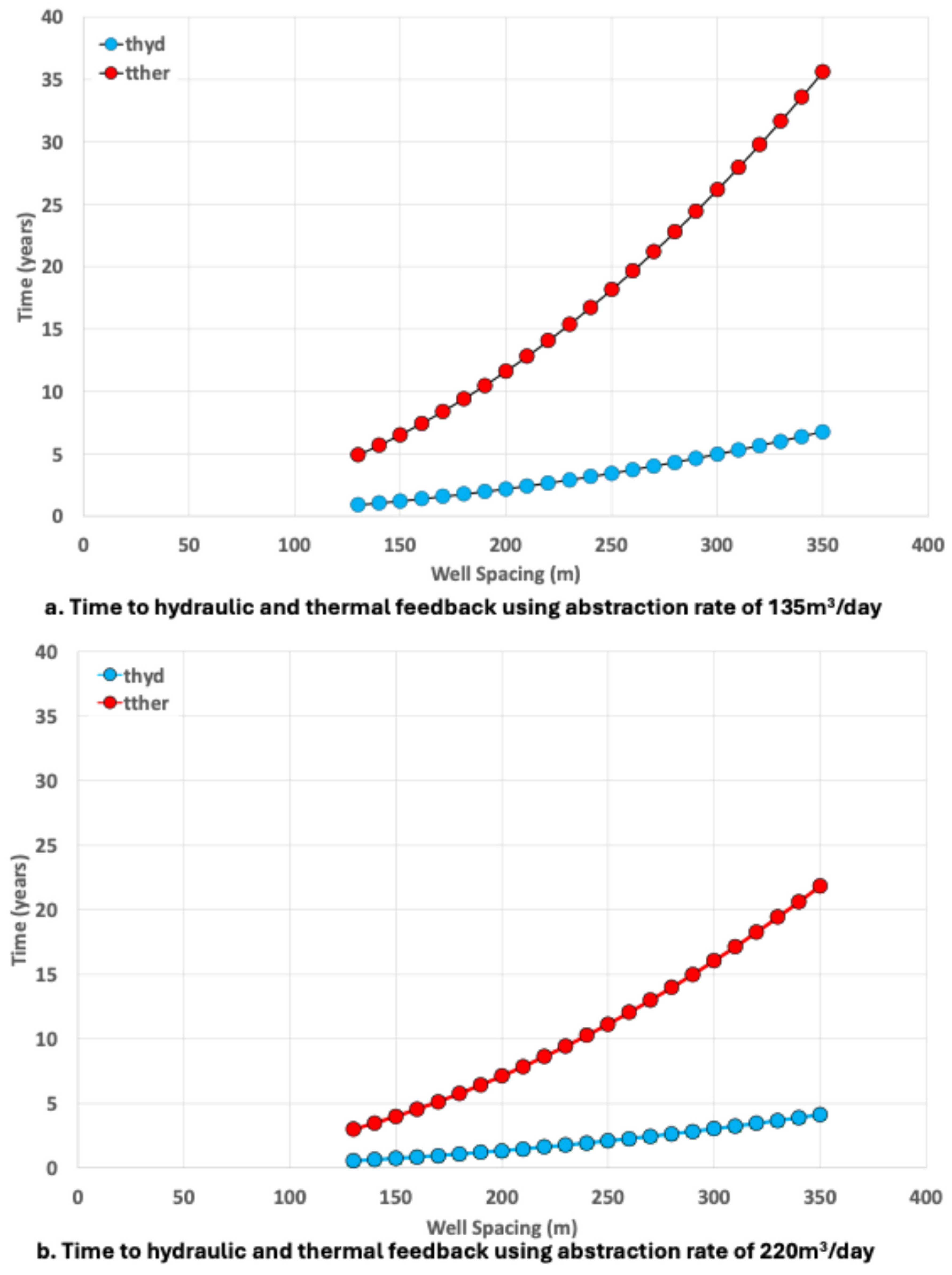
Using the equations in Section 2.2, an estimate of hydraulic and thermal feedback time has been made. Figure 23 demonstrates the effect of increasing well spacing on feedback times, for a system abstracting at the required rates for only the Lido (a), and for the Lido and surrounding sports facilities (b).

Figure 23. Plots of well spacing against time to hydraulic and thermal feedback for heating and cooling of only Ilkley Lido (a), and for the Lido and surrounding sports facilities (b).

The time to thermal feedback can be significantly increased by maximising the well spacing, with an increase between minimum and maximum spacing of around 20 years for a system supporting the Lido and surrounding facilities.

However, applying these idealised empirical formulas directly to the heterogeneous Marchup Grit introduces distinct physical biases. While Equations (6) and (7) calculate breakthrough assuming an infinite, homogeneous 2D aquifer with uniform matrix advection, the actual subsurface environment at Ilkley is governed by fracture networks, structural compartmentalisation, and variable ambient gradients. Consequently, these analytical estimates serve primarily as a baseline screening envelope that must be cross-examined against both site-specific structural conditions and numerical modelling.

7. Finite Element Modelling of Flow

A representative FEM has been built in COMSOL Multiphysics version 6.0 [32] to approximate fluid and heat flow within the target aquifer of Mp and surround MGS, through a net heating GSHP scheme based on the feasibility study. Fluid flow is approximated through Darcys Law, and heat flow through advection, dispersion, and conduction. The model investigates the change over a period of ten years as an initial estimate of aquifer development during implementation. This period is suitable, as making assumptions far into the future could lead to erroneous conclusions, given that most data used in this study are not truly representative of the actual site conditions and are an approximation.

The model is a simplified version of the geometry at the Lido, with a flat topography, no change in the dip angle of the beds, and with no interaction with faults. This approach was taken because of computational restrictions on processing power, and ultimately due to time constraints. Due to this and the underlying assumptions regarding material properties, the model should not be used as an explicit solution for flow dynamics in the aquifer but is suitable as a starting point to understand the dynamics of the aquifer, and how they might change over time. The model also allows comparison of results from empirical estimates of thermal breakthrough times.

Finite element numerical modelling was implemented to overcome the inherent physical limitations of empirical breakthrough formulas. While analytical equations assume instantaneous thermal equilibrium and 1D advective travel, the coupled FEM framework in COMSOL Multiphysics resolves transient 2D Darcian flow coupled with simultaneous conductive, advective, and dispersive heat transfer. The simplified geometry was adopted to isolate primary doublet hydrodynamic–thermal interactions under constrained boundary conditions, serving as an initial benchmark prior to 3D discrete-fracture modelling.

7.1. Model Configuration

The chosen geometry has been simplified and depicts a doublet arrangement with a spacing of 130 m as a worst-case scenario. The model extents were selected to give a suitable distance from the well locations, but without being too far as to increase computation times unnecessarily. The boundaries were set to ‘open’ on the y-axis for the Darcian flow module and closed on the x-axis, effectively making the upper and lower boundaries impermeable. The heat transfer within porous media module was set in the same manner, so that model boundaries were also open to heat flow along the y-axis and closed on the x-axis.

The material parameters outlined in the previous sections of this study were used to estimate material properties in the model, albeit lowered slightly to account for uncertainties with data collection and the extent of fracturing within the target aquifer. The mesh setup was configured for fluid dynamics and was set to extra fine, giving a maximum element size of 2.73 m and minimum size of 3.15 mm, with smaller element sizes populating the areas of the model where flow conditions may be more dynamic. Overall, the model setup is justified for the purpose of the study and objectives of the modelling, which is as an initial estimate of the flow conditions in the aquifer over time.

To ensure full model transparency and reproducibility, the complete configuration of the 2D finite element numerical simulation is summarised in Table 15. The model couples Darcy’s Law for fluid dynamics with heat transfer in porous media within COMSOL Multiphysics. Lateral model boundaries (y-axis) were assigned open hydraulic heads matching the regional hydraulic gradient (i = 0.01) alongside convective heat outflow conditions, while the upper and lower boundaries (x-axis) were specified as impermeable and thermally insulated to isolate the doublet exchange within the local sedimentary sequence. An extra-fine triangular mesh was generated with severe refinement surrounding the 130 m spaced abstraction and reinjection wellbores (minimum element size of 3.15 mm), grading to a maximum element size of 2.73 m in the far field. Grid independence testing confirmed that doubling element resolution altered simulated breakthrough temperatures by less than 0.5%.

Table 15. Finite element numerical model configuration and simulation parameters in COMSOL Multiphysics [32].

Category	Parameter/Feature	Specified Value	Units	Governing Law/Implementation Basis
Domain Geometry	Domain Dimensions (X × Y)	460 × 210	m	Sized laterally to eliminate boundary-effect interference on flow lines
	Target Aquifer Thickness (D)	30	m	Marchup Grit sandstone layer between −80 m and −110 m depth
	Overburden Strata	80	m	Millstone Grit Shale (MGS) confining low-permeability caprock
	Underburden Strata	100	m	Basal Millstone Grit Shale extending to base of model (−210 m)
	Doublet Well Spacing (L)	130	m	Conservative minimum spacing constrained by site boundaries
Hydraulic Setup	Governing Flow Formulation	Darcy’s Law	—	∇ · (ρ u) = Q_m, where u = −(κ/μ) ∇p
	Aquifer Horizontal Hyd. Conductivity (Kh)	1.2 × 10−3	m/day	Field-derived equivalent continuous porous medium (ECPM)
	Aquifer Vertical Hyd. Conductivity (Kv)	4.0 × 10−4	m/day	Vertical anisotropy ratio (Kv = Kh/3)
	Confining Shales Hyd. Conductivity	1.0 × 10−6	m/day	Low-permeability aquitard representation
	Abstraction/Injection Flow Rate (Z)	135	m3/day	Matched to peak space heating demand of Ilkley Lido complex (1.56 L/s)
	Natural Regional Hydraulic Gradient (i)	0.01	—	Regional southeasterly gradient applied as constant-head boundary condition
	Hydraulic Boundary Conditions	Open (y)/Closed (x)	—	Specified head at lateral boundaries; impermeable no-flow top and bottom
Thermal Setup	Heat Transfer Formulation	Porous Media Heat Transfer	—	(ρ Cp)_eff (∂T/∂t) + ρ_f Cp_f u · ∇T = ∇ · (λ_eff ∇T)
	Target Aquifer Baseline Temperature	14.5	°C	Estimated in situ fluid temperature at ~90 m bgl
	Injected Fluid Temperature	10.0	°C	Δθ = 4.5 K temperature drop across GSHP evaporator circuit
	Sandstone Thermal Conductivity (λs)	3.75	W/(m·K)	Matrix baseline derived from core lithology literature
	Shale Thermal Conductivity (λsh)	1.80	W/(m·K)	Lower thermal conductivity of confining boundary mudstones
	Aquifer Volumetric Heat Capacity (SVCaq)	2.20	MJ/(m3·K)	Sandstone matrix volumetric heat capacity
	Fluid Volumetric Heat Capacity (SVCw)	4.18	MJ/(m3·K)	Standard thermophysical properties of groundwater
	Geothermal Gradient	0.026	°C/m	Applied as initial linear thermal condition across model depth
	Thermal Boundary Conditions	Open (y)/Closed (x)	—	Convective outflow at lateral boundaries; thermally insulated top and base
Mesh and Solver	Mesh Type	Triangular (Extra Fine)	—	Physics-controlled mesh tailored for fluid dynamics
	Element Dimensions	Min: 3.15 mm; Max: 2.73 m	—	Strong refinement around well boundaries; relaxed in far field
	Total Mesh Elements	~48,500	—	Mesh convergence confirmed: doubling elements caused <0.5% thermal variance
	Time-Stepping Solver	PARDISO (Transient)	—	Backward differentiation formula (BDF), 0 to 10-year operational span

7.2. Results and Analysis

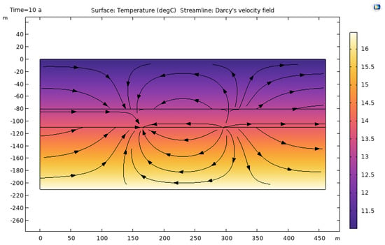
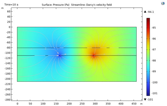
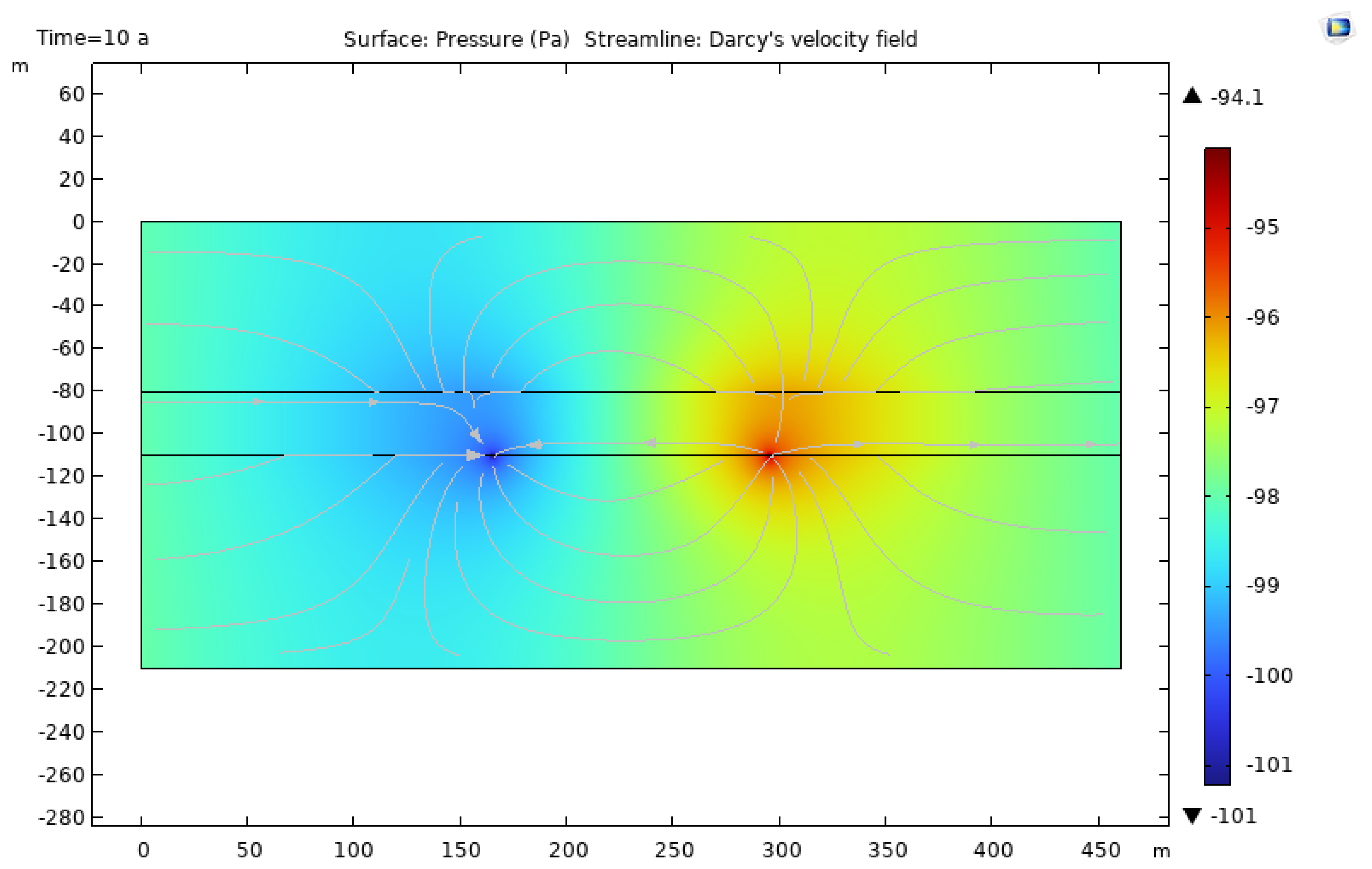
The flow field overlying the natural geothermal gradient at the point of implementation is illustrated in Figure 24.

Figure 24. Initial flow field and geothermal gradient at start of abstraction and injection, with the abstraction well on the left and injection well on the right.

The pressure field conditions are stable with time and do not vary considerably from zero years to ten years (Figure 25). This is because the injection well increases pressures while the abstraction well reduces them, which has a net effect of stabilising pressures.

Figure 25. Theoretical flow field after 10 years of operation.

An induced flow direction to the abstraction well from the injection well occurs at the start of abstraction, as the wells will lower and elevate the hydraulic head, respectively, in their immediate surroundings, which causes an induced hydraulic gradient between the wells.

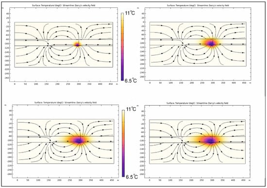
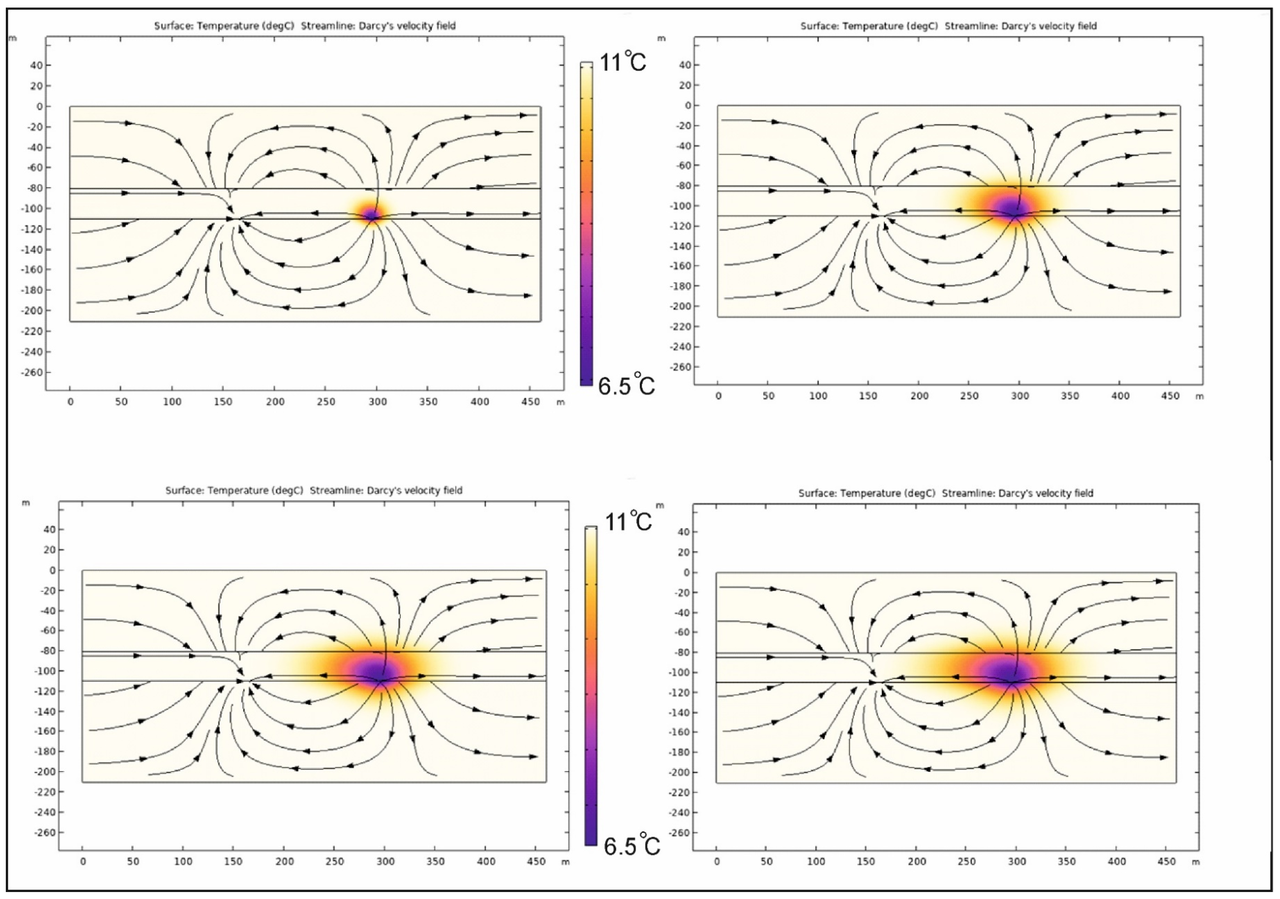
Over time, the development of a cooler water plume occurs from one year to ten years, as illustrated in Figure 26. The plots show the change in temperature between a stable background temperature of the surrounding rock mass and the cooler plume of water, which is reinjected at a temperature reduced by 4.5 °C after utilisation in the GSHP scheme. The cooled water steadily migrates from the injection well on the right to the abstraction well on the left, along the induced hydraulic gradient. Based on these plots, the time at which thermal breakthrough will occur is at around eight to ten years from initial implementation.

Figure 26. Plots of thermal plume development over time. At one year (top left), five years (top right), eight years (bottom left), and ten years (bottom right).

The results of numerical modelling have shown that if injection and abstraction rates are matched, overall pressures will have no net change. The results of pressure distribution are as expected and are likely to hold true in practice, on the proviso that injection and abstraction rates are maintained at the same rate.

Based on the plots of temperature flow, migration of the cooled injection water is likely to occur after around 9 to 10 years. Migration of the cooled groundwater takes longer than expected in the model when compared to the empirical analysis of breakthrough times. This is likely because the numerical model considers the natural laws of dispersion, advection, and conduction in calculation of heat flow, whereas the empirical method is a simplified assessment. Therefore, the results from the FEM analysis can be assumed to provide a more conservative value for breakthrough times compared to results from empirical analysis.

While empirical equations calculate thermal breakthrough based solely on 1D advective travel times, the finite element model incorporates 2D hydrodynamic dispersion, thermal conduction into adjacent low-permeability strata, and buoyant fluid mixing. Consequently, the apparent delay in numerical breakthrough (8–10 years at 130 m spacing) compared to empirical formulas (4.5 years at 130 m spacing) reflects the inclusion of multi-directional thermal diffusion. However, in the absence of site-specific transient pump test calibration, both numerical and analytical estimates should be interpreted as complementary screening envelopes rather than definitive predictions.

Many simplifications and assumptions have been made to build the model and analyse the results, including simplifying the geometries, along with assuming thermal, geological, and hydrogeological parameters of the expected strata. In addition, the heterogeneity and anisotropy of both the Mp and MGS will play a major role in the flow of heat and fluids. The model does not consider the variability in the Mp or MGS below the formation scale. Increased flow and, therefore, reduced breakthrough times, could be possible where extensive fracturing occurs, which will increase permeability within the Mp. The omission of fault structures in the 2D continuum model represents a fundamental simplification. As established in the 3D conceptual model, fault shear zones (such as those observed adjacent to BH12) can exhibit fracture densities significantly higher than the host sandstone mass. If a doublet array intersects a continuous, high-permeability fault corridor aligned along the hydraulic gradient, preferential channelling will occur, potentially accelerating thermal breakthrough significantly faster than predicted by matrix-dominated simulations. Consequently, ignoring high-permeability faults risks overestimating operational breakthrough longevity. Conversely, fault gouge development or fault-induced juxtaposition of sandstone against impermeable Millstone Grit Shales would induce reservoir compartmentalisation, restricting yield and accelerating localised drawdown. The fieldwork undertaken during this study demonstrated that the aquifer shows some anisotropy with variable thicknesses of sandstone that have different porosities, strengths, and slightly different fracture networks. The MGS also contains thin sandstone beds, which could increase permeabilities further if fractures connect these beds up- and down-sequence.

8. Discussion of Key Findings

The study has shown the range of estimated depths to the base of each expected formation in the study area, within approximately 1 km below ground level. Shear zones around the inferred faults of the area could act as barriers or conduits for fluid flow. Overall, evidence of upwelling of groundwater along shear zones points towards the fault zones in the study area increasing fluid flow. Fieldwork identified two main joint sets with high persistence within the Mp and identified anisotropy within the formation between two units of sandstone.

The Mp aquifer was selected as the most suitable target based on the depth to strata (~90 m), reasonable transmissivity estimates, and modest subsurface temperatures (~14.5 °C). Pump tests indicate a range of transmissivities between 4 m²/day and 58 m²/day, with a mean of 25.8 m²/day. Temperatures in the WWG could be ~21.5 °C and around ~33.4 °C in the Pdl.

A combined heat demand of 104 kW was estimated to supply peak heating requirements for the Lido and Rugby Club, which corresponds to a required flow rate of 220 m³/day. A flow rate of 135 m³/day would be suitable to meet peak demand for the Lido building space heating only.

Drawdowns in an open-loop well system within the Mp could reach the top of the aquifer or even deplete the aquifer depending on the prevailing transmissivity beneath the study area. Drawdowns of between 17 m and 110 m, and 11 m and 68 m, are estimated, based on pump rates of 220 m³/day and 135 m³/day, and the lowest and average transmissivity values, respectively.

Using a doublet (abstraction and injection well), optimal well spacing is estimated at around 290 m to 940 m and is limited to a maximum of ~350 m due to space restrictions. Thermal feedback times at a well spacing of 300 m may be in the region of 26 to 16 years, based on an abstraction/injection rate of 135 m³/day and 220 m³/day, respectively. FEM demonstrated that the actual feedback times are likely to be higher, with breakthrough times at around 8 years for a well spacing of 130 m, compared to around 4.5 years when using empirical methods.

To critically appraise whether analytical calculations remain valid under these in situ conditions, several competing geological mechanisms must be considered:

• Fracture networks vs. matrix flow: Analytical formulas distribute flow uniformly across an assumed effective bulk porosity. Outcrop surveys, however, demonstrate that flow in the Marchup Grit is governed by persistent sub-vertical joint sets (J1 and J2). Where connected fracture corridors bridge the doublet, localised advective velocity will exceed bulk matrix velocity, potentially causing initial cold-water breakthrough earlier than predicted by Equations (6) and (7).
• Fault juxtaposition and compartmentalisation: Analytical solutions assume an infinite boundary domain. At Ilkley, normal faulting can throw sandstone against thick mudstone/shale aquitards (MGS), truncating lateral reservoir continuity. Placing both wells within a narrow, fault-bounded graben restricts available aquifer volume and accelerates thermal recycling.
• Hydraulic gradient uncertainty: Critical spacing and stagnation points (Equation (5)) are sensitive to the ambient hydraulic gradient, which is estimated between 0.01 and 0.034 based on regional boreholes. Lower ambient gradients diminish natural downstream advective flushing, thereby expanding the recirculating capture zone between the doublet wells.
• Conductive thermal buffering from aquitards: In contrast to the accelerating effects of fractures, analytical equations completely neglect conductive heat transfer from adjacent confining units. The low-permeability Millstone Grit Shales bounding the aquifer act as continuous conductive thermal reservoirs, replenishing heat into the sandstone matrix. This physical buffering counteracts cold-plume development and delays systemic temperature drops—a mechanism absent in empirical piston-flow equations but captured by numerical finite element modelling.

The most suitable aquifer for exploitation of shallow geothermal energy is Mp. If further space heating as part of a geothermal cluster would be considered, abstractions within the Mp may be suitable, but deeper, thicker strata (WWG) should also be considered, as the potential yields from a BH within the Mp may not be large enough to sustainably operate a well system abstracting over 190 m³/day. However, uncertainty regarding geometry and physical properties of deeper strata, such as WWG, is higher due to lack of data.

The sustainability of the systems can be improved by maximising well spacing. At the highest possible well spacing (based on limitations on space) of 350 m, thermal breakthrough times are much larger, at around 22 to 36 years. As the FEM analysis has shown, these values should be taken as conservative estimates and are likely to be higher in practice, indicating that a sustainable open-loop well system is feasible in the Mp at the given abstraction rates.

From a techno-economic perspective, open-loop doublet configurations exhibit distinct capital expenditure (CAPEX) and operational expenditure (OPEX) trade-offs compared to closed-loop borehole heat exchangers (BHEs). Meeting the 104 kW peak space heating demand via a closed-loop array would require approximately 15 to 20 vertical boreholes drilled to depths of 100–150 m, representing a substantial upfront capital drilling expenditure. Conversely, an open-loop scheme significantly reduces initial drilling CAPEX by utilising only two dedicated doublet wells targeted into the Marchup Grit (~90–115 m depth). However, open-loop systems incur higher ongoing OPEX, including parasitic electrical consumption from submersible abstraction pumps, regular mechanical maintenance, and water filtration to mitigate mineral scaling or particulate clogging. Furthermore, thermal breakthrough directly impacts operating costs: a 2 °C decline in abstraction fluid temperature degrades heat pump COP by approximately 4–6%, progressively increasing annual grid electricity consumption and lengthening the payback period. Modulating the system design to supply 70% of the peak thermal load minimizes initial pump ratings and capital sizing while effectively buffering against premature thermal depletion.

The conceptual ground model outlines the assumed architecture of the study area based on surface mapping and borehole logs. The surface mapping is not entirely reliable, as superficial coverage of the study area is widespread and most of the boundaries are inferred. Additionally, when building the 3D model, it was clear that some of the boundaries were incorrect due to the 3D geometries below the surface being unfeasible because of high dip angles. Boreholes are inconsistently distributed, and the quality of information is highly variable, with many of the logs only containing a drillers description of the bore. This could result in some unquantified heterogeneity and anisotropy within the formations, as detailed logging is not available. The effect of these issues is that the model geometries are not entirely reliable, although they are suitable as an initial estimate and to guide assessment of geothermal heating potential.

Faults can act as barriers and can induce compartmentalisation in aquifers where aquicludes/aquitards are adjacent to the aquifers. Lithofacies, diagenesis, dissolution features, and fractures have a major role in reservoir quality [12,13]. The model highlights areas where aquitards are adjacent to the aquifer but the nature of the fracture network is not completely understood, which could result in increased or decreased flows. Based on all the information in this study, increased flows seem likely, as a high degree of fracturing is recorded near shear zones in MGS, along with calcite veins and changes in groundwater chemistry, but this cannot be confirmed until site-specific investigations are conducted.

The calculation of the geothermal gradient and subsequent subsurface temperatures was undertaken using regional heat fluxes, assumed thermal properties, and relied upon the depth to the base of each formation from the conceptual model and literature. Given that the conceptual model has inherent inaccuracies, and that thermal properties are not obtained directly, the estimates also have an appreciable level of uncertainty attached. Uncertainty increases with depth to each formation, as borehole records do not extend beyond 152 m in the study area, and the thicknesses of the deeper formations (WWG and Pg in particular) can vary by 100–200 m.

Flow rates are estimated based upon the heat demand and assume a COP of 4 and boiling point of refrigerant at 7 °C. This will result in variations in the required flow rates, as they are dependent on the actual refrigerant and COP of the unit used in any system, along with expected subsurface temperatures. The COP value and boiling points are standard for GSHP systems [12] and are reasonable to assume. Although the other variables are less certain, the flow rates are suitable initial estimates.

Optimal well spacing, expected drawdowns, and thermal feedback hold much more uncertainty in their estimation owing to the density and quality of hydrogeological data, methods of analysis, and assumptions that apply to the underlying equations. The flows in the region are dominated by fracture networks, and where these are not present, flow is reduced significantly [15,26]. The range of these estimates is highly variable due to the range of transmissivities in the study area, which is related to the fracture network.

The parameter baseline adopted in the numerical modelling (Table 15) reflects central conservative estimates; however, the actual subsurface domain is subject to substantial parametric uncertainty, as documented across Table 2, Table 3 and Table 4, and 8. Critical hydrogeological sensitivity is governed by the wide transmissivity bounds (4 to 58 m²/day). Under the lower-bound transmissivity (4 m²/day), peak abstraction yields excessive drawdowns (S_w = 68 m at 135 m³/day and S_w = 110 m at 220 m³/day), which would pull the piezometric surface below the top of the confined Marchup Grit horizon (~88 m depth), triggering mineral precipitation and severe borehole dewatering. Conversely, at mean or upper-bound transmissivities (T >= 25.8 m²/day), drawdown remains manageable (S_w <= 17 m), confirming that hydrodynamic viability hinges on intersecting transmissive fracture corridors. Furthermore, variations in effective fracture aperture (0.5 to 1.5 mm at depth vs. 4.8 mm at surface outcrop; Table 6), effective porosity (6% to 19.2%; Table 7), and regional hydraulic gradient (0.01 to 0.034; Figure 12) collectively modulate the calculated analytical thermal feedback window between 16 and 36 years. These sensitivities underscore that while the system is conditionally feasible, exploratory borehole drilling and multi-rate pumping tests are indispensable to pinpoint localised transmissivity before finalising pump specifications and depth settings.

The [21] method of calculating transmissivities is suitable in non-leaky, confined aquifers, where pump tests fully penetrate the aquifer and steady-state conditions are not reached. Although the aquifer is confined, leakage will occur through fracture networks, and some of the tests did not fully penetrate Mp, so these assumptions do not hold true. The actual values of transmissivity are unknown below most of the study area and the range is large, so estimates could be proven to be inaccurate following investigation of the actual conditions.

Thermal feedback estimates are uncertain because of the reasons above but are more constrained by using FEM analysis, which produced results that concur with the empirical analysis. Despite this, the simplification of the FEM model and exclusion of fracture networks also results in the possibility of lower or higher thermal breakthrough times in practice. Movement along fractures will result in higher flows and will mean that some of the cooled water will reach the abstraction well before the main plume [12]. The dynamics of the aquifer may also change with time. Decrease of formation pore pressure because of depletion will increase effective stresses and cause the apertures (widths) of the hydraulic fractures to reduce; therefore, fracture conductivity decreases [18]. The risk of this occurring is tangible if the fracture network around the injection well permits loss of pressure due to higher transmissivities.

In addition to the above, artesian groundwater conditions could have a beneficial impact on the system by decreasing the amount of energy input required to pump from an abstraction well but could also introduce difficulties in the injection well. The effect of this should be considered.

Overall, the findings of this study point towards an open-loop well system within the Mp being conditionally feasible, based upon the synthesised preliminary data. Reducing the design flow rates to match 70% of the peak thermal demand offers a viable mitigation pathway to delay thermal breakthrough and preserve heat pump efficiency. Nonetheless, because these conclusions rest on generalised regional parameters, idealised boundary conditions, and uncalibrated models, the system cannot be designated as definitively viable at this screening stage. Detailed intrusive investigations—specifically exploratory coring, on-site multi-rate pumping tests, and hydrochemical analysis—are essential prerequisites before finalising engineering designs or committing capital.

9. Concluding Remarks

This feasibility study has processed and collated open-access information from the BGS to assess the potential for a GSHP at the study area in Ilkley. The shallow ground conditions comprise variable superficial deposits to a maximum depth of around 25 mbgl near the Lido, with Carboniferous Millstone Grit shales and sandstones below. Potential targets for exploitation though GSHP’s include the Marchup Grit at around 90 mbgl, possibly deeper grit formations, and Pendleside Limestone at depths of >700 mbgl.

Fieldwork at outcrops of the Marchup Grit demonstrated that the formation is variable between two sandstone units, and analysis of data in the literature showed yields required in an open-loop doublet to match the heat demand of the Lido and surrounding facilities could be met. However, the sustainability of the system may be impacted by thermal feedback from an injection well. Reducing the overall output to match 70% of space heating demand, along with maximising spacing, could improve sustainability in the long term. Thermal feedback is estimated to occur within approximately 22 years when utilising an optimal spacing of 300 m based on analytical calculations but reduces to 8–10 years under a spatially constrained spacing of 130 m, as demonstrated by transient finite element numerical modelling (at 135 m³/day).

Sustainable abstraction rates should be pursued to allow adequate time to recoup upfront capital costs and make any project cost-efficient. Further investigation can aid in characterising the ground conditions and refining designs, as well as allowing for full appreciation of the potential impacts to the local groundwater regime.

Using FEM to further refine the estimated hydrogeological regime and assess thermal feedback should be undertaken. The model in this report is simplified and, therefore, future modelling should include more representative site geometries, account for fractures and faults, and ideally include results from investigations.

In addition, regional studies show the potential for geothermal systems in Carboniferous limestones [9,26]. However, there is a lack of specific information regarding flows in the region to be able to come to tangible conclusions at the study area. Further work should assess these units to the northwest of Ilkley, specifically aiming to characterise the fractures at outcrop, and possibly using borehole records in other areas of the UK as an analogy for the expected conditions beneath the study area.

In conclusion, while the shallow Marchup Grit demonstrates conditional feasibility as a low-carbon geothermal source, field development should proceed with caution. Definitive confirmation of system viability will ultimately require on-site borehole drilling, hydrochemical characterisation to assess scaling potential, and calibrated long-duration pumping tests to substantiate long-term hydrodynamic and thermal sustainability.

References

- Ng, C.; Paraskevopoulou, C.; Shaw, N. Stability Analysis of Mineshafts used for Minewater Heat Recovery in the UK. Geotech. Geol. Eng. 2019, 37, 5245–5268. [Google Scholar] [CrossRef] [Scilit]
- Agrawal, M.; Zurita, M.; Paraskevopoulou, C.; Admiraal, H.; Cornaro, A.; Gupta, A. Underground Urbanism: Re-Imagining the Role of Underground Spaces for India’s Urban Future; National Institute of Disaster Management (NIDM), Ministry of Home Affairs, Government of India: Delhi, India, 2022; p. 39.
- Green, N.; Paraskevopoulou, C.; Branham, E.; Clarke, R.; Shaw, N. Using legacy data to investigate the geothermal potential of UK’s aquifers: A feasibility study at the University of Leeds, UK. Geoenergy Sci. Eng. 2025, 254, 214025. [Google Scholar] [CrossRef] [Scilit]
- Paraskevopoulou, C.; Cornaro, A. Utilising the subsurface for sustainable green energy solutions—Potential examples from the UK. In Proceedings of the 19th World Conference of the Associated Research Centers for the Urban Underground Space (ACUUS 2025), Belgrade, Serbia, 4–7 November 2025. [Google Scholar]
- Gehringer, M.; Loksha, V. Geothermal Handbook: Planning and Financing Power Generation; Energy Sector Management Assistance Program (ESMAP) Technical Report 002/12; The World Bank: Washington, DC, USA, 2012. [Google Scholar]
- Farr, G.; Busby, J.; Wyatt, L.; Crooks, J.; Schofield, D.I.; Holden, A. The temperature of Britain’s coalfields. Q. J. Eng. Geol. Hydrogeol. 2020, 54, 20–109. [Google Scholar] [CrossRef] [Scilit]
- Paraskevopoulou, C.; Connolly, A.; Kearsey, T.; Shaw, N. Utilising the Subsurface for Sustainable Green Energy Solutions. In Underground Spaces for Climate Resilience and Sustainability; Agrawal, M., Ed.; Advances in 21st Century Human Settlements; Springer: Singapore, 2025; pp. 115–138. [Google Scholar] [CrossRef] [Scilit]
- Jones, D.J.R.; Randles, T.; Kearsey, T.; Pharaoh, T.C.; Newell, A. Deep geothermal resource assessment of early carboniferous limestones for Central and Southern Great Britain. Geothermics 2023, 109, 102649. [Google Scholar] [CrossRef] [Scilit]
- Busby, J. Geothermal energy in sedimentary basins in the UK. Hydrogeol. J. 2014, 22, 129–141. [Google Scholar] [CrossRef] [Scilit]
- Digimap. Digimap Onshore Mapping Service; EDINA, University of Edinburgh: Edinburgh, UK, 2023; Available online: https://digimap.edina.ac.uk (accessed on 10 July 2023).
- Thain, I.; Reyes, A.G.; Hunt, T. A Practical Guide to Exploiting Low Temperature Geothermal Resources; GNS Science Report 2006/09; GNS Science: Wairakei, New Zealand, 2006; 76p. [Google Scholar]
- Banks, D. An Introduction to Thermogeology: Ground Source Heating & Cooling, 2nd ed.; John Wiley & Sons Ltd.: Chichester, UK, 2012. [Google Scholar]
- Moeck, I.S. Catalog of geothermal play types based on geologic controls. Renew. Sustain. Energy Rev. 2014, 37, 867–882. [Google Scholar] [CrossRef] [Scilit]
- Sarbu, I.; Calin, S. General Review of Ground-Source Heat Pump Systems for Heating and Cooling of Buildings. Energy Build. 2014, 70, 441–454. [Google Scholar] [CrossRef] [Scilit]
- Abesser, C. Open-Loop Ground Source Heat Pumps and the Groundwater Systems: A Literature Review of Current Applications, Regulations and Problems; British Geological Survey Open Report OR/10/045; BGS: Keyworth, UK, 2007; 31p. [Google Scholar]
- Lund, J.W.; Freeston, D.H.; Boyd, T.L. Direct utilization of geothermal energy 2010 worldwide review. Geothermics 2011, 40, 159–180. [Google Scholar] [CrossRef] [Scilit]
- Clyde, C.G.; Madabhushi, G.V. Spacing of Wells for Heat Pumps. J. Water Resour. Plan. Manag. 1983, 109, 203–212. [Google Scholar] [CrossRef] [Scilit]
- Zhang, J.J. Applied Petroleum Geomechanics: Chapter 2—Rock Physical and Mechanical Properties; Elsevier: Cambridge, MA, USA, 2019; pp. 45–98. [Google Scholar] [CrossRef] [Scilit]
- British Geological Survey (BGS). GeoIndex Onshore Portal; BGS: Keyworth, UK, 2023; Available online: https://mapapps2.bgs.ac.uk/geoindex/home.html (accessed on 12 August 2023).
- Australian Geothermal Energy Group (AGRC). The Geothermal Reporting Code: Australian Code for Reporting of Exploration Results, Geothermal Resources and Geothermal Reserves, 2nd ed.; Australian Geothermal Energy Association: Unley, SA, Australia, 2010. [Google Scholar]
- Cooper, H.H.; Jacob, C.E. A generalized graphical method for evaluating formation constants and summarizing well field history. Trans. Am. Geophys. Union 1946, 27, 526–534. [Google Scholar] [CrossRef] [Scilit]
- Aydin, A. ISRM Suggested Method for Determination of the Schmidt Hammer Rebound Hardness: Revised Version. Int. J. Rock Mech. Min. Sci. 2008, 45, 25–33. [Google Scholar] [CrossRef] [Scilit]
- Aitkenhead, N.; Barclay, W.J.; Brandon, A.; Chadwick, R.A.; Chisholm, J.I.; Cooper, A.H.; Johnson, E.W. British Regional Geology: The Pennines and Adjacent Areas, 4th ed.; HMSO for the British Geological Survey: London, UK, 2002. [Google Scholar]
- Waters, C.N. Geology of the Bradford District—A Brief Explanation of the Geological Map Sheet 69 Bradford (England & Wales); Sheet Explanation of the British Geological Survey; BGS: Keyworth, UK, 1999. [Google Scholar]
- Morton, A.C.; Whitham, A.G. The Millstone Grit of northern England: A response to tectonic evolution of a northern source land. Proc. Yorks. Geol. Soc. 2002, 54, 47–56. [Google Scholar] [CrossRef] [Scilit]
- Abesser, C.; Shand, P.; Ingram, J. Baseline Report Series: 18. In The Millstone Grit of Northern England; British Geological Survey Commissioned Report No. CR/05/015N; BGS: Keyworth, UK, 2005. [Google Scholar]
- Jones, H.K.; Morris, B.L.; Cheney, C.S.; Brewerton, L.J.; Merrin, P.D.; Lewis, M.A.; MacDonald, A.M.; Coleby, L.M.; Talbot, J.C.; McKenzie, A.A.; et al. The Physical Properties of Minor Aquifers in England and Wales; British Geological Survey Technical Report WD/00/4; Environment Agency R&D Publication 68; BGS: Keyworth, UK, 2000; 234p. [Google Scholar]
- Bernward Hölting, B.; Coldewey, W.G. Physicochemical Processes in Groundwater Flow; Springer Textbooks in Earth Sciences, Geography and Environment; Springer: Berlin/Heidelberg, Germany, 2018. [Google Scholar] [CrossRef] [Scilit]
- Glover, P.W.J.; Zadjali, I.I.; Frew, K.A. Permeability prediction from MICP and NMR data using an electrokinetic approach. Geophysics 2006, 71, 49–60. [Google Scholar] [CrossRef] [Scilit]
- Reyes, A.G. Petrology of Philippines geothermal systems and the application of alteration mineralogy to their assessment. J. Volcanol. Geotherm. Res. 1990, 43, 279–309. [Google Scholar] [CrossRef] [Scilit]
- Schout, G.; Griffioen, J.; Hassanizadeh, S.M.; de Louw, P.G.B. Impact of stray gas on groundwater quality in a multi-layered aquifer system. Sci. Total Environ. 2020, 705, 135834. [Google Scholar]
- COMSOL AB. COMSOL Multiphysics® Reference Manual, Version 6.0; COMSOL AB: Stockholm, Sweden, 2021. [Google Scholar]
Disclaimer/Publisher’s Note: The statements, opinions and data contained in all publications are solely those of the individual author(s) and contributor(s) and not of MDPI and/or the editor(s). MDPI and/or the editor(s) disclaim responsibility for any injury to people or property resulting from any ideas, methods, instructions or products referred to in the content. |
© 2026 by the authors. Licensee MDPI, Basel, Switzerland. This article is an open access article distributed under the terms and conditions of the Creative Commons Attribution (CC BY) license.