


Abstract
Long-duration diesel engine condition monitoring requires vibration descriptors that remain comparable over time despite path-dependent structural responses and physical measurements acquired on different schedules. A methodological need therefore remains for transparent multi-location screening followed by retention of one unchanged descriptor across a complete endurance sequence. This study develops an evidence chain workflow using a 300 h WP4.6 whole-engine endurance test at 2100 r/min and 600 N·m. In a representative synchronized record, cylinder pressure and nine vibration channels were sampled at 200 kHz, while complete eleven-node longitudinal histories were available only for liner X/Y/Z. After operating boundary and record integrity checks, multi-domain screening selected cylinder-2 Liner-Y 3–7 kHz integrated band power and retained this definition unchanged across all endurance nodes. The descriptor increased overall from 78.57 to 613.68 a.u.2 (; Spearman ) but remained non-monotonic, including a 40.0% decrease from 180 to 210 h. Mean cumulative bearing shell loss progressed from 3.126 to 6.590 and 10.776 mg at 100, 200, and 300 h, while post-test liner geometry showed a self-referenced circumferential-mean peak of 12.17 m and maximum ovality of 26.67 m. These non-equivalent physical measurements provide complementary context rather than synchronized wear labels. The workflow therefore supports auditable long-duration response screening and inspection prioritization for the present engine–sensor configuration, without establishing calibrated wear prediction or universal transferability of the selected channel or frequency band.
1. Introduction
The durability of a diesel engine depends in part on the condition of its principal friction pairs. The cylinder liner–piston ring interface governs combustion-chamber sealing, piston guidance, and oil control, while the crankshaft–bearing shell interface supports cyclic gas and inertia loads through lubricated sliding contact. During prolonged operation, both interfaces are exposed to changing pressure, motion, lateral force, temperature, and lubrication. Bore geometry, surface inspection, component weighing, lubricant analysis, and wear-debris examination can reveal accumulated condition [1,2,3,4,5,6,7,8]; however, these measurements are normally obtained at maintenance or disassembly stages. They provide direct or outcome-based physical evidence but do not preserve the temporal evolution of the running engine during an uninterrupted endurance test.
Vibration monitoring can fill part of this temporal gap because measurements can be repeated without interrupting the test. Engine-surface vibration has been used to characterize combustion events [9,10,11,12,13], and the relation between cylinder pressure and external structural response makes combustion an excitation reference rather than an interchangeable durability metric [9,10,11,14]. Interpretation nevertheless remains inseparable from the operating boundary: combustion, valve train impacts, reciprocating inertia, piston secondary motion, shaft dynamics, and structural resonances overlap in multi-source, non-stationary signals. Changes in speed, torque, or thermal and lubrication state may therefore appear as changes in a candidate durability feature [15]. Transmission path and sensor placement can likewise alter the measured response [16,17]. A recent diesel engine monitoring review identifies non-stationarity, noise, operating condition dependence, and sensor placement as persistent challenges across contemporary processing approaches [16]. Dynamic signals must therefore be interpreted with retained operating variables and explicit limits on what the measured response can represent [18,19].
Piston slap and liner-local vibration provide a more direct basis for near-source observation. Piston lateral motion and impact have been related to measurable vibration and noise [20,21,22,23,24], while vibration and acoustic emission studies show that severe liner or piston scuffing can produce detectable high-frequency responses [25,26,27]. Measurements near the block and liner support observations closer to the source [28,29,30], although liner vibration can also couple with fluid and structural phenomena such as cavitation [31]. Transmission path studies further show that sensor locations are not physically interchangeable. Measurements near the combustion wall and main-bearing region have resolved multiple pathways for combustion-induced vibration [17], and recent piston–liner transmission modeling likewise supports path-aware interpretation [32]. Liner-adjacent vibration is therefore physically relevant, but neither a long-term increase nor a selected band uniquely identifies one internal mechanism.
Transmission path and sensor selection must consequently form part of the analysis. A far-field sensor can integrate several structural paths, whereas a near-source direction can be amplified or attenuated by local stiffness, mounting geometry, and directional load transfer. The X, Y, and Z liner signals are directional projections rather than statistical replicates, and the largest short-record amplitude is not necessarily the most useful long-term response. Sensor and feature selection should therefore be evaluated jointly from response distinguishability, physical position, record integrity, and longitudinal coverage.
The selected signal representations serve complementary purposes. Time-domain statistics summarize amplitude and impulsiveness, whereas the fast Fourier transform and Welch power spectral density support transparent spectral screening and a reproducible fixed-band integrated power definition. The continuous wavelet transform (CWT) provides multiscale localization of non-stationary oscillatory morphology; the complex Morlet wavelet is used here as a practical oscillatory analyzing wavelet rather than a demonstrated optimum. The CWT maps were independently normalized and were therefore used only for qualitative morphology rather than absolute cross-channel amplitude comparison; the normalization procedure is specified in Section 2.4. The short-time Fourier transform (STFT) provides a fixed time–frequency grid for band-occupancy visualization and the supplementary high-energy-area ratio (HEAR), with the expected fixed-window resolution trade-off. Fourier-domain and wavelet analyses can thus provide complementary views [33], while general rotating machinery evidence describes the trade-offs between fixed-window and multiresolution methods [34]. Because wavelet representation and derived features can depend on the mother wavelet and decomposition settings [35], the final longitudinal feature is not selected from absolute CWT amplitude. Order/cyclic analyses, adaptive decomposition, deconvolution, and data-driven classification address rotation-normalized events, mode or source separation, or fault recognition [36,37,38,39,40,41]; the present objective is instead to retain one interpretable descriptor under one processing definition throughout a scheduled multi-hundred-hour endurance sequence.
Prior work has combined diesel engine vibration with post-test component mass loss and liner-surface evidence in hot-engine wear studies [42]. Extended engine health monitoring has also paired repeated vibration measurements with less-frequent lubricant property and chemical measurements, preserving different observation schedules across evidence domains [43]. Together with recent work on diesel engine condition monitoring and transmission path characterization [16,17,33], these studies establish a basis for cross-domain condition assessment. Comparatively limited methodological attention, however, has been given to transparently screening multiple structural vibration channels over a multi-hundred-hour whole-engine endurance test, reducing them to one channel–frequency-band descriptor, and retaining its definition across every scheduled node while preserving the original, non-equivalent observation schedules of the physical evidence.
The engineering question is therefore whether an auditable screening procedure can identify one configuration-specific vibration descriptor, freeze its definition after selection, and retain it throughout a complete 300 h endurance sequence while keeping subsequent physical evidence on its true observation basis. This study addresses that question using a WP4.6 four-cylinder diesel engine. The representative comparison includes nine synchronized vibration channels, whereas complete eleven-node longitudinal histories are available only for liner X/Y/Z. The analysis proceeds from record integrity, operating boundary, and combustion-repeatability checks to multi-location time-domain and spectral comparison, qualitative CWT and fixed-grid STFT examination, channel–feature screening, longitudinal evaluation over the eleven measured liner nodes, and bounded comparison with bearing shell mass loss and post-test liner geometry.
Three evidence-backed contributions follow. First, an auditable multi-location screening framework combines operating boundary checks, record integrity, structural position, within-record response comparison, and complete endurance-node coverage for candidates entering longitudinal ranking so that channel selection is not determined by single-record amplitude alone; in the present dataset, only liner X/Y/Z have complete eleven-node histories. Second, after retrospective screening within the available endurance sequence, one configuration-specific channel–frequency-band descriptor is selected; its channel identity, frequency limits, and processing definition are then frozen and kept unchanged across all eleven endurance nodes. The contribution lies in definition-invariant longitudinal retention rather than universal transfer of the selected direction or band. Third, feature selection is separated from subsequent physical interpretation: bearing shell mass loss and post-test liner geometry are compared with the vibration trajectory on their actual observation schedules, without interpolation into artificial synchronized wear labels or feedback into feature definition. This is a schedule-preserving methodological safeguard rather than a new signal-processing algorithm. For the present engine–sensor configuration, this procedure ultimately identifies Liner-Y 3–7 kHz integrated band power as the retained longitudinal descriptor. The resulting evidence provides bounded cross-domain physical context for a durability-sensitive vibration response; it does not establish calibrated wear prediction, continuous wear reconstruction, unique-source attribution, or universal transferability.
2. Experimental System, Measurements, and Analysis Framework
This section converts the evidence chain defined in the Introduction into a reproducible acquisition and analysis protocol. The organization follows the experimental order: Section 2.1 defines the engine, endurance condition, and recorded operating boundary; Section 2.2 defines the synchronized pressure–vibration hierarchy; Section 2.3 preserves the actual timing and form of the wear evidence; Section 2.4 specifies the conventional signal analyses; and Section 2.5 states the channel–feature decision rules and statistical limits. This order ensures that operating conditions and excitation references are established before a vibration channel or feature is selected.
2.1. Test Engine, Endurance Protocol, and Operating Records
The experiment was conducted on a WP4.6 four-cylinder diesel engine installed on a whole-engine endurance platform. The complete engine, rather than an isolated component, was tested so that combustion excitation, reciprocating inertia, shaft-system coupling, structural transmission, lubrication, cooling, and dynamometer loading remained present. The prescribed endurance duration was 300 h at a nominal operating condition of 2100 r/min and 600 N·m. The fixed speed–load point was prescribed by the endurance protocol before vibration analysis and was retained to reduce operating condition uncertainty in within-test comparison; it was not selected retrospectively to optimize the 3–7 kHz response. The test-cell control system recorded speed, torque, temperatures, pressures, and environmental variables. The six retained test-cell records characterize the observed operating envelope of the endurance program; they do not constitute node-by-node operating verification for all eleven vibration measurements. Their numerical comparability is evaluated in Section 3 rather than assumed here.
The complete experimental design combined the 300 h endurance chain with a synchronized dynamic hierarchy centered on cylinder 2: cylinder pressure provided an excitation reference, liner X/Y/Z provided near-source responses, and cylinder head and main-bearing-region X/Y/Z provided structurally transmitted responses. The three evidence streams retained their actual measurement schedules. Vibration was recorded at 11 nodes from 0 to 300 h, bearing shells were weighed at 100, 200, and 300 h, and liner geometry was surveyed post-test; consequently, 300 h is the only exact vibration–bearing overlap. Figure 1 documents the actual whole-engine endurance test bench, multichannel data acquisition hardware, and representative sensor installations at the main-bearing region and Cylinder-2 liner.
Figure 1.
Representative photographs of the 300 h whole-engine endurance test and vibration measurement system: (a) whole-engine endurance test bench; (b) multichannel data acquisition hardware; (c) main-bearing-region sensor installation; and (d) Cylinder-2 liner accelerometer installation. All panels show the actual experimental setup.
As listed in Table 1, the retained equipment records identify a Kistler 6052C cylinder pressure sensor, an OMRON E6B2-CWZ5G crank angle encoder, a Donghua Testing DH8303 high-speed acquisition system, and 1A313E three-axis vibration sensors. The engine was manufactured by Weichai Power Co., Ltd. (Weifang, China); the CE52HA dynamometer was supplied by Hangzhou Yike Electromechanical Technology Co., Ltd. (Hangzhou, China); the 6052C pressure sensor by Kistler Instrumente AG (Winterthur, Switzerland); the E6B2-CWZ5G encoder by OMRON Corporation (Kyoto, Japan); and the DH8303 acquisition system and 1A313E vibration sensors by DongHua Testing Technology Co., Ltd. (Jingjiang, China). Cylinder pressure and vibration were sampled synchronously at 200 kHz. The model identifiers make the acquisition chain traceable, while the functional column states how each item contributes to the evidence sequence used in the subsequent analysis.
Table 1.
Principal test object and measurement equipment.
2.2. Synchronized Dynamic Measurement Layout
The synchronized measurement hierarchy separated the recorded quantities into reference, near-source, and structurally transmitted levels. Cylinder-2 pressure (AI2-23) formed the combustion reference level and was used to assess local event timing and within-record cycle repeatability. Cylinder-2 liner vibration formed the near-source level, with X/Y/Z retained as AI1-29/AI1-28/AI1-30. Cylinder head X/Y/Z (AI1-19/AI1-20/AI1-21) and main-bearing-region X/Y/Z (AI2-05/AI2-06/AI2-07) formed the upper- and lower-structure transmission levels. The crank angle encoder supplied the phase reference but was not treated as a condition feature.
The second cylinder was used because the retained test configuration combined cylinder pressure measurement with local three-axis liner sensing at that cylinder. The cylinder head and main-bearing-region signals were not substitutes for the liner signal; they were included to determine whether a large response originated near the liner or reflected a different transmission path. This distinction is essential because combustion, piston–liner interaction, valvetrain excitation, cranktrain motion, and structural resonances may contribute simultaneously to an external vibration record.
The liner X, Y, and Z signals were treated as directional projections under a common excitation environment, and no direction was designated as the main channel before analysis. In the project coordinate definition, liner Y is oriented in the crankshaft-axial direction from the free end toward the flywheel. Table 2 links each retained channel group to its measured quantity and admissible analytical role; the channel identifiers are included so that every plotted response can be traced back to the acquisition record.
Table 2.
Synchronized measurement hierarchy and interpretation boundaries.
The hierarchy is intended to prevent path-amplified responses from being interpreted as source-specific condition evidence and to prevent separately scheduled physical measurements from being treated as synchronized condition labels.
The distinction between near-source and structurally transmitted responses was maintained throughout interpretation. A change in a liner channel was therefore not automatically assigned to liner wear, and a change near the main-bearing region was not automatically assigned to bearing shell wear. The subsequent physical measurements provide stage-level and terminal component condition context for the endurance-scale vibration evolution; they are not treated as source-specific validation of the vibration feature.
2.3. Measurement Schedule and Physical Wear Evidence
As specified in Table 3, the dynamic and physical measurements were available on different schedules and in different data forms. Vibration records were retained at eleven nominal endurance nodes from 0 to 300 h in 30 h increments. Bearing shell weighing was available only at 100, 200, and 300 h, and cylinder-2 liner geometry was measured after completion of the endurance test. Stating these schedules before analysis prevents the datasets from being made artificially synchronous by interpolation or by creation of unmeasured values.
Table 3.
Measurement schedule, data form, and permitted comparison.
For bearing position j and weighing stage h, the cumulative combined shell mass loss was calculated from the recorded pre-test upper- and lower-shell masses as
where the masses are in grams and is in milligrams. Differences between successive measured stages were calculated only as and . The pre-test masses are calculation references for material loss; they are not an independently observed 0 h bearing-wear node. Therefore, no “relative-to-0 h bearing wear” trajectory, fitted wear law, or significance claim was constructed. Moreover, the 30 h vibration schedule does not contain exact 100 or 200 h records. Only 300 h is shared exactly by both schedules, so the 100 and 200 h evidence is compared by stage order and interval context rather than by interpolated synchronous pairs.
The cylinder-2 liner survey contained eight diameter lines from 0 to 157.5 in 22.5 increments, 37 retained measurement heights below the top-chamfer exclusion region, and three repeat readings at each line–height point. Because each diameter line represents an unoriented axis, major-axis angles are defined modulo 180; accordingly, 157.5 is equivalent to . A fixed robust aggregation rule was applied to all 296 repeat triplets before spatial summaries were formed. If the range of a triplet was no greater than 3 m, its arithmetic mean was retained; if the range exceeded 3 m, its median was retained. The 3 m threshold was the 90th percentile of the observed triplet-range distribution and was applied uniformly rather than adjusted point by point. Under this rule, 28 of 296 triplets (9.46%) were median-processed. For the non-flagged triplets, the median residual standard error was 0.333 m; the corresponding repeatability-only estimate for a self-referenced difference was 0.471 m. These values characterize repeat dispersion in the retained survey and are not used to reconstruct an unmeasured pre-test bore map.
Each diameter line was then referenced to its own minimum robust value. The circumferential-mean relative geometry at each height was calculated as the mean of the eight line-specific relative values, whereas ovality was calculated as the maximum minus minimum of the eight robust diameters at that height. This self-referencing removes line offsets but also prevents the result from being interpreted as absolute wear depth. Because no pre-test bore map was available, the liner evidence describes only the final height-dependent and circumferentially non-uniform geometry; it cannot establish when that geometry developed or how much material was removed during each endurance interval.
The pressure, vibration, and phase reference channels within the representative high-rate dynamic record were acquired synchronously. This synchronization does not extend to every evidence stream over the full 300 h campaign: the eleven-node liner X/Y/Z longitudinal vibration histories, six retained test-cell records, bearing shell weighing stages, and post-test liner survey retain their respective observation schedules. Cross-domain comparisons therefore preserve the actual measurement times and do not create artificial synchronous pairs.
2.4. Signal Preprocessing and Conventional Analyses
The analysis was intentionally ordered from conventional signal descriptions to feature selection. All signal preprocessing, screening, and feature calculations reported in this study were performed offline as post-processing of retained records; no inline or real-time implementation was evaluated. Each retained vibration record was checked for finite values, usable length, abnormally low-amplitude or dropout behavior, local saturation, and gross broadband contamination, after which the retained signal was demeaned. The exported vibration amplitudes were retained in the arbitrary units of the acquisition chain; comparisons therefore apply within this fixed chain, and no calibrated acceleration magnitude is claimed. Absolute amplitude differences among structural locations are interpreted only within the present acquisition chain and should not be read as calibrated structural-transfer gains. Two analysis scales were kept distinct. The synchronized waveform and CWT comparisons use the same 20 ms (4000-sample) excerpt from one representative record so that channel shapes are compared on a common time base. In contrast, the eleven-node RMS, PSD-derived integrated band power, and HEAR sequences were calculated from each node’s full retained exported segment. No missing endurance node was filled, no bearing stage was interpolated, and records were not resampled or truncated to manufacture equal-duration observations. The full node segments contained 2,052,479–3,890,420 samples (10.262–19.452 s), corresponding to 249–473 complete Welch windows under the reported 16,384-sample window and 8192-sample overlap. Across the retained liner X/Y/Z longitudinal subset, the eleven endurance nodes comprise 84,862,092 scalar vibration samples in total. This total refers only to the retained liner X/Y/Z longitudinal vibration subset and should not be interpreted as the size of the complete experimental dataset, which additionally includes other dynamic channels, operating records, and physical inspection data. Density normalization, frequency bins, and the 3–7 kHz integration limits were fixed across nodes; segment length therefore changed the number of Welch averages, not the spectral or feature definition.
Time-domain screening used root-mean-square (RMS), absolute peak amplitude, and Pearson kurtosis. For a demeaned record with N samples, RMS was calculated as
Frequency-domain screening began with the discrete Fourier transform. To reduce the sensitivity of a single-periodogram display to finite-window fluctuations, the reported power spectral density (PSD) was estimated by Welch averaging with a 16,384-sample Hann window, 8192-sample overlap, 16,384-point FFT, and one-sided density normalization. Linear PSD is reported in a.u.2/Hz. Logarithmic spectra use one common arbitrary reference across channels and are used only for visual comparison; no calibrated decibel quantity is claimed.
For any candidate interval , integrated band power was calculated from the linear PSD as
The resulting integrated band power has units of a.u.2. The 3–7 kHz interval was retained as a fixed empirical candidate band from the representative multi-channel spectral comparison and physically relevant medium-to-high-frequency ranges reported in piston slap and liner contact studies [22,23,32]. The cited studies motivate examination of this region, while the exact interval remains specific to the present engine–sensor configuration. Applying one fixed definition across all nodes makes the subsequent comparison reproducible and auditable; global bandwidth optimization was outside the scope of this screening study.
For the representative record, the descriptive 3–7/0.5–7 kHz integrated power ratio was defined as
This dimensionless ratio was used as a descriptive screening dimension for spectral concentration, but not as a stand-alone criterion for final channel–feature selection.
Two time–frequency methods were used to examine whether spectral energy was persistent or concentrated in local events. Continuous wavelet analysis used a complex Morlet wavelet with on representative windows and a 1–20 kHz display grid. For display, each CWT map was normalized independently by the 95th percentile of power in that channel; colors therefore support within-panel morphology assessment but not absolute cross-panel power comparison. Short-time Fourier transform (STFT) used a 512-sample Hann window, 50% overlap (256 samples), a 256-sample step, and a 512-point FFT. STFT power was obtained as the one-sided squared FFT magnitude normalized by the Hann-window energy; the interior one-sided bins were doubled, and no logarithmic conversion was used for HEAR. Representative maps supported channel and feature interpretation, while HEAR was calculated from the full retained Liner-Y segment at every vibration node. Neither the map morphology nor HEAR was converted into a wear quantity.
Morlet CWT was used as a practical oscillatory analyzing wavelet for qualitative multiscale localization of transient vibration structures; it is not claimed to be optimal. A different mother wavelet could alter time–frequency localization, effective resolution, morphology, local amplitude, and any wavelet-derived features, so invariance across wavelets is not assumed. STFT and CWT serve complementary roles: STFT provides a fixed, reproducible time–frequency grid suitable for cross-record comparison and HEAR visualization, with a fixed-resolution trade-off, whereas CWT provides multiscale localization but depends on the selected wavelet and scale mapping. The final longitudinal descriptor is therefore not selected from absolute CWT amplitude.
For a supplementary scalar description of the STFT, the high-energy area ratio (HEAR) was defined as
where is the linear, window-energy-normalized STFT power at endurance node h. The implemented 3–7 kHz interval contained ten discrete bins spanning 3125–6640.625 Hz. The threshold was calculated once from the 0 h band-power bins using the population standard deviation and then held fixed for all nodes. The fixed is a baseline-relative engineering reference rather than an optimized multivariable or universal alarm threshold. Deployment-level threshold calibration would require healthy-population data across engines and operating conditions together with explicit false-alarm and missed-detection assessment. This engineering definition identifies time–frequency activity above the typical 0 h baseline level. HEAR and RMS are complementary descriptions of the same Liner-Y response rather than independent validation of the integrated band power descriptor.
2.5. Channel–Feature Selection and Descriptive Statistics
The analysis followed a fixed decision sequence. First, the retained operating records characterized the available operating envelope, and the cylinder pressure record established within-record repeatability. Second, synchronized time-domain, FFT/Welch–PSD, CWT, and STFT results were compared across the liner, cylinder head, and main-bearing-region channels. Third, only channels with adequate record integrity and sufficient endurance-node coverage entered long-term comparisons. Fourth, candidate features were evaluated across the eleven vibration nodes. Finally, the selected vibration sequence was placed beside the bearing shell and liner evidence on their actual observation schedules.
The nine synchronized vibration channels entered the representative common-window and spectral comparisons. Complete eleven-node histories were retained only for liner X/Y/Z; consequently, longitudinal ranking and the final channel choice were restricted to those three directions, while the head and main-bearing-region channels served as representative transmission path contrasts.
Main channel selection was not based on the largest instantaneous amplitude. A candidate had to satisfy five criteria: (1) usable record integrity; (2) a consistent physical location and direction; (3) distinguishability from far-field structural responses in the common-window comparison; (4) complete coverage of the eleven measured endurance nodes; and (5) a feature trend that was interpretable under fixed processing parameters. The main feature was selected only after conventional analyses in the time, frequency, and time–frequency domains. Overall RMS and HEAR were retained as complementary descriptors when they helped determine whether the primary trend was a broadband amplitude effect or a persistent band-limited change.
The channel–feature pair was selected retrospectively from the complete eleven-node vibration sequence. Slope, , and Spearman were used as descriptive within-test ranking statistics. Bearing shell and liner measurements were retained on their actual observation schedules and used as cross-domain physical context rather than artificially synchronized targets. Accordingly, the analysis provides an engineering screening result for the present test configuration rather than an out-of-sample predictive model.
Retained project scripts and tabulated outputs were used for signal processing and figure regeneration. Together with the equations and schedules reported above, the project analysis record preserves the fixed sampling frequency, transform parameters, band limits, channel identifiers, node schedules, and wear calculation rules used in this study.
3. Operating Boundary and Multi-Channel Feature Screening
This section implements the selection logic established in Section 2. The record audit retained complete eleven-node histories for all three liner directions, whereas the cylinder head and main-bearing-region channels were available only for representative synchronized comparisons; no absent long-term record was filled. With that availability boundary established, Figure 2 first constrains the operating and local combustion reference boundary. Figure 3, Figure 4 and Figure 5 then compare the synchronized channels in the time, frequency, and time–frequency domains without presupposing a preferred direction. Figure 6 connects the representative STFT to an explicit channel–feature matrix, and Table 4 together with Figure 7 complete the decision using all eleven endurance nodes. This order separates candidate-band identification from final feature selection and prevents the main channel from being chosen solely because it has the largest amplitude in one record.
Figure 2.
Operating and combustion reference boundaries: (a) speed and torque across six retained test-cell records; (b) thermal-variable means ± standard deviations and full ranges; (c) pressure-variable means ± standard deviations and full ranges; and (d) cycle-wise peak-pressure sequence and distribution for the representative 448-cycle synchronized record. In panel (d), the dashed horizontal line marks the mean peak pressure of 15.373 MPa. Panels (a–c) constrain the retained operating envelope, whereas panel (d) establishes repeatability only within the displayed record.
Figure 3.
Representative 20 ms (4000-sample) time-domain comparison of nine synchronized vibration channels: (a–c) cylinder-2 liner X/Y/Z; (d–f) cylinder head X/Y/Z; and (g–i) main-bearing-region X/Y/Z. RMS, absolute peak, and Pearson kurtosis are reported for the same displayed window. Colors are used only to distinguish the plotted channel traces and do not encode an additional quantitative variable. The comparison shows that directional waveform structure and measurement position, rather than amplitude alone, must enter the channel decision.
Figure 4.
FFT/Welch frequency-domain comparison: (a) liner direction PSD levels; (b) representative Y-direction PSD levels at the liner, cylinder head, and main-bearing region; and (c) 3–7 kHz integrated band power for all nine channels. The shaded region marks the candidate band. All PSD curves use one common arbitrary reference, so the logarithmic levels are comparative rather than calibrated decibels. The largest integrated band power occurs outside the liner and is not used as the selection criterion.
Figure 5.
Morlet CWT comparison over the common 20 ms window and 1–20 kHz grid: (a–c) liner X/Y/Z; (d) cylinder head Y; and (e) main-bearing-region Y. Dashed lines mark 3 and 7 kHz. Power is normalized separately by the 95th percentile of each channel and therefore represents within-channel organization rather than cross-channel magnitude. Main finding: the CWT panels distinguish transient morphology across structural locations but do not independently select Liner-Y.
Figure 6.
STFT and initial channel–feature screening: (a) approximately 180 ms Liner-Y STFT with 3 and 7 kHz boundaries; (b) maximum band bin power per frame shown against the fixed 0 h HEAR threshold, which is applied to every linear 3–7 kHz time–frequency bin; and (c) screening matrix for long-term completeness, the descriptive 3–7/0.5–7 kHz integrated power ratio, linear integrated band power trend , and Spearman . For the cylinder head and main-bearing-region channels, N/A denotes no complete 11-node longitudinal series, not absence of representative synchronized data; an em dash in a trend cell denotes that the channel is not eligible for longitudinal ranking. Main finding: only liner X/Y/Z satisfy complete eleven-node longitudinal coverage, and Liner-Y provides the strongest eligible long-term ordering.
Table 4.
Complete record-screening and descriptive trend evidence for liner direction selection. All three rows contain values at the eleven measured nodes; the X statistics are reported only as a non-ordered audit reference. “Power” denotes the 3–7 kHz integrated band power defined in Equation (3).
Figure 7.
Eleven-node comparison of the two positively ordered liner directions: (a) RMS sequences; (b) 3–7 kHz integrated band power sequences; and (c) normalized slope, linear-fit , and Spearman descriptors used for the Y/Z decision. For visualization only, the integrated band power slopes in panel (c) were normalized by the larger absolute value of the Y/Z integrated band power slopes. All measured Y and Z nodes, including the local maxima at 180 h, are retained. Main finding: compared with Liner-Z, Liner-Y provides the stronger combined longitudinal ordering and is therefore retained as the primary channel.
3.1. Operating Boundary and Within-Record Combustion Repeatability
The first analytical step was to characterize the nominal loading boundary represented by the available slow-variable records. As shown in Figure 2a, the six retained test-cell records were tightly grouped around the prescribed speed and torque. The mean speed was 2100 ± 1 r/min, with a range of 2098–2101 r/min, and the mean torque was 600.0 ± 0.1 N·m, with a range of 599.9–600.1 N·m. Thus, the retained records show small speed and load deviations relative to the 2100 r/min and 600 N·m set points. They characterize the observed operating envelope but do not provide node-by-node verification for all eleven vibration measurements.
Figure 2b,c define the accompanying thermal and pressure envelope. The coolant outlet temperature was 81.1 ± 1.3 C, the oil temperature was 108.6 ± 2.4 C, and the oil pressure was 445.5 ± 9.1 kPa. By comparison, the ambient temperature covered 28.9–47.6 C and the fuel temperature covered 39.5–71.6 C. The figure therefore establishes stable dynamometer loading and bounded auxiliary conditions for the retained records, while preserving the wider environmental and fuel temperature variation as part of the test boundary.
Figure 2d provides a separate check of cycle-to-cycle repeatability within the representative synchronized record used for the local channel comparison. Its 448 detected cycles had a mean peak pressure of 15.373 MPa, a sample standard deviation of 0.091 MPa, and a coefficient of variation of 0.595%. The narrow distribution supports treating this record as a common local combustion reference for Figure 3, Figure 4, Figure 5 and Figure 6. Because this evidence comes from one record, it does not establish invariant combustion across all endurance nodes; cylinder pressure is used as an excitation reference rather than as a liner condition feature.
3.2. Representative Time-Domain Comparison Across Nine Vibration Channels
Figure 3 compares all nine synchronized vibration channels over the same 20 ms interval. The liner X, Y, and Z directions had RMS values of 30.03, 22.96, and 29.61 a.u., respectively, and Pearson kurtosis values of 4.49, 6.06, and 4.68. Their absolute peaks were 142.73, 136.16, and 153.69 a.u., respectively. Each direction contained an impulsive response packet near the middle of the window, but the amplitude, polarity distribution, and decay pattern differed. The three liner axes therefore represent distinct directional projections of the same operating event rather than interchangeable replicate measurements.
The largest response occurred outside the liner. Cylinder head Z reached an RMS of 74.86 a.u., and main-bearing-region Z reached 92.81 a.u.; the latter was 3.09 times the Liner-X RMS in the same window. These channels occupy different structural positions and transmission paths; their higher amplitudes therefore reflect a path-dependent response and are insufficient for liner sensitivity selection. Figure 3 consequently motivates the separation of near-source liner responses from upper-structure and crankcase path responses.
3.3. FFT/Welch Spectral Comparison and Candidate-Band Definition
The same channels were next compared in the frequency domain using Welch-averaged PSD. As shown in Figure 4a, the liner directions have visibly different spectral organization inside the candidate 3–7 kHz interval. Their integrated band power values were 288.25, 71.29, and 286.26 a.u.2 for X, Y, and Z, respectively. Liner-Y had the smallest local band magnitude in this representative record; its later selection therefore arose from the longitudinal criteria rather than from the largest initial candidate-band response.
Figure 4b,c further separate local spectral structure from propagation path magnitude. Cylinder head Z had a 3–7 kHz integrated band power of 391.47 a.u.2, whereas the main-bearing-region X, Y, and Z values were 422.13, 1592.25, and 5884.71 a.u.2. The nearly two-order spread across the nine channels shows that absolute integrated band power is strongly dependent on measurement position and structural transmission. The 3–7 kHz interval was retained because it provided a common, distinguishable spectral region for subsequent fixed-parameter comparison, but neither its single-record magnitude nor its broadband fraction was used alone to select the main channel.
3.4. Morlet CWT Comparison of Transient Spectral Organization
Figure 5 applies the Morlet CWT to five channels over the same 20 ms window used for the time-domain comparison and on a common 1–20 kHz frequency grid. The liner directions show different transient organizations: Liner-Z develops a comparatively sustained 3–7 kHz response after approximately 10 ms, whereas Liner-Y contains a more localized band response accompanied by short high-frequency activity. Cylinder head Y shows a pronounced high-frequency burst, while main-bearing-region Y contains broader, more distributed activity inside the candidate band. These differences reinforce that direction and propagation path alter the time–frequency response; the panels are not scaled copies of one waveform.
Each CWT panel was normalized by the 95th percentile of its own channel power. The colors therefore preserve the timing and frequency organization within a channel but cannot be compared as absolute power across panels. Figure 5 consequently serves as a morphology check: it shows why a fixed scalar criterion is still required, but it does not by itself select Liner-Y.
Together, Figure 3, Figure 4 and Figure 5 show why the conventional analyses precede feature selection. Time-domain statistics describe amplitude and impulsiveness, Welch spectra identify candidate frequency intervals, and CWT reveals transient organization. Long-term availability and node-level ordering then complete the endurance channel decision.
3.5. STFT Description and Transparent Channel–Feature Screening
Figure 6a extends the local analysis from the 20 ms comparison window to an approximately 180 ms Liner-Y STFT. Repeated broadband events and band-limited activity cross the dashed 3 and 7 kHz boundaries, showing that the candidate interval is occupied repeatedly rather than being defined by one isolated Fourier peak. In Figure 6b, the line shows the maximum 3–7 kHz bin power in each time frame only to visualize the fixed threshold. The threshold itself is the mean plus one population standard deviation of all 0 h linear band-power bins and is applied to every corresponding time–frequency bin at every endurance node; HEAR is the percentage of bins exceeding it.
Figure 6c summarizes long-term completeness, the descriptive 3–7/0.5–7 kHz integrated power ratio, and the longitudinal ordering statistics. All three liner directions have 11 long-term nodes. By contrast, the retained cylinder head and main-bearing-region channels support the synchronized representative comparison but have no complete 11-node longitudinal series, which is why their completeness cells read N/A and they are not eligible for longitudinal ranking. For the liner directions, the descriptive ratios of 3–7 kHz integrated band power to 0.5–7 kHz integrated band power were 0.369 for X, 0.192 for Y, and 0.666 for Z. The lowest ratio belongs to Y; this value is reported as a descriptive screening dimension for spectral concentration and was not used as a stand-alone criterion for final channel–feature selection.
The long-term integrated band power descriptors provide the decisive separation. Liner-X produced and Spearman ; Liner-Y produced and ; and Liner-Z produced and . Figure 6c therefore identifies Liner-Y as the leading candidate because it combines a near-source position and complete node coverage with the strongest ordered 3–7 kHz integrated band power sequence. Section 3.6 then checks this decision against the full directional histories rather than accepting the matrix alone.
The screening values are descriptive summaries of one measured engine–sensor sequence. Because the candidate ranking and the displayed endurance histories use the same eleven nodes, they document a traceable retrospective within-test selection rather than an independently validated ranking across engines or installations. The subsequent Section 4 history is therefore a descriptive presentation of the selected response, not a holdout or validation result.
3.6. Long-Term Directional Comparison and Primary Feature Selection
The full directional histories were inspected before the main channel decision. All three liner axes contain values at the eleven nominal nodes, and at each node, the X, Y, and Z features were calculated from exported segments of equal duration; segment duration varied jointly among nodes from 10.26 to 19.45 s, giving 249–473 complete Welch windows per node. Liner-X nevertheless showed strong reversals: its RMS was 12.40, 64.97, 14.57, and 8.38 a.u. at 120, 210, 240, and 300 h, respectively, while its 3–7 kHz integrated band power ranged from 11.34 a.u.2 at 300 h to 1508.90 a.u.2 at 210 h. Because no independent in situ sensitivity record is available to distinguish directional physics from installation or record effects, these values are shown without smoothing for audits and are treated as a non-ordered directional reference rather than as evidence of wear reversal.
Table 4 reports the complete descriptive statistics for all three directions, including the X values rather than suppressing them after inspection. Liner-Y and Liner-Z both show positive RMS slopes, but the Y-direction integrated band power sequence has substantially higher linear and rank ordering. The coefficients describe the measured vibration response under the retained installation; they are not material loss rates.
Figure 7 then compares the two directions with positive overall trend descriptors across the eleven measured nodes. Figure 7a,b show the Y- and Z-direction RMS and 3–7 kHz integrated band power histories, while Figure 7c places normalized slope, linear-fit , and Spearman on one decision scale. Liner-X remains visible in Figure 6c and Table 4; it is omitted from Figure 7 only so that the final Y/Z comparison is not visually dominated by its 210 h excursion.
Figure 7a,b preserve the local fluctuations in both directions. Liner-Y RMS increased from 26.47 to 44.16 a.u. between 0 and 300 h, with a descriptive slope of 0.0572 a.u./h, , and Spearman . Liner-Z RMS changed from 30.40 to 39.57 a.u.; its slope was 0.0429 a.u./h, with and . Both directions reached a local maximum at 180 h and decreased at 210 h. The final decision therefore depends on overall ordering across all nodes while retaining the measured non-monotonic behavior.
The band-limited comparison provides the clearest separation. Liner-Y 3–7 kHz integrated band power increased from 78.57 to 613.68 a.u.2, with a slope of 1.689 a.u.2/h, , and . Liner-Z changed from 324.00 to 396.55 a.u.2, but its was 0.103 and was 0.555. After the common 180 h local maximum, Z-direction integrated band power remained within approximately 383–397 a.u.2 from 210 to 300 h, whereas Y-direction integrated band power rose from 353.58 to 613.68 a.u.2 over the same nodes.
The evidence chain therefore converges on cylinder-2 Liner-Y as the main channel and its 3–7 kHz integrated band power as the primary feature. The decision is supported jointly by complete node coverage, near-source position, the strongest integrated band power rank ordering, and an accompanying positive RMS trend rather than by the largest representative amplitude or band fraction. Liner-Y RMS is retained as a complementary overall-amplitude descriptor, and HEAR is retained as a supplementary time–frequency descriptor derived from the same signal. This selection defines the 0–300 h response-tracking analysis for the present engine, coordinate definition, sensor installation, acquisition chain, and fixed processing settings.
4. Evolution of the Primary Feature over 300 h
With the selected channel–feature definition carried forward unchanged from Section 3, Figure 8 presents the eleven-node cylinder-2 Liner-Y history as primary 3–7 kHz integrated band power in Figure 8a, complementary broadband RMS in Figure 8b, and supplementary time–frequency occupancy (HEAR) in Figure 8c. All three descriptors were calculated from the same retained Liner-Y records without interpolation, smoothing, or point removal.
Figure 8.
Measured evolution of the selected cylinder-2 Liner-Y response over 0–300 h: (a) primary 3–7 kHz integrated band power; (b) complementary RMS; and (c) supplementary HEAR derived from the same vibration records. Dashed lines are descriptive least-squares fits. In panel (a), the blue filled markers highlight the 0 h and 300 h endpoints; the open circular markers denote the measured endurance nodes. All eleven nodes are retained, showing the overall upward ordering, the local peak at 180 h, and the common decrease at 210 h.
4.1. Primary 3–7 kHz Integrated Band Power Evolution
Figure 8a traces the selected 3–7 kHz integrated band power through the full endurance sequence. The response rose from 78.57 a.u.2 at 0 h to 308.62 a.u.2 at 90 h. A modest decrease of approximately 6% occurred from 90 to 120 h, from 308.62 to 290.24 a.u.2, after which the response increased to 352.05 a.u.2 at 150 h and 589.26 a.u.2 at 180 h. The largest local reversal occurred from 180 to 210 h when integrated band power decreased by 40.0% from 589.26 to 353.58 a.u.2. After 210 h, the feature increased to 446.64, 504.95, and 613.68 a.u.2 at 240, 270, and 300 h, respectively; the 300 h value exceeded the 180 h local maximum.
Across the endpoints, the net increase was 535.1 a.u.2, or 681.1% relative to the 0 h value, and eight of the ten adjacent intervals increased. The descriptive least-squares slope was 1.689 a.u.2/h with ; the rank association with endurance time was Spearman . Thus, both endpoint separation and node ordering support an overall upward evolution, whereas the two observed decreases show that the response was neither monotonic nor adequately represented as a smooth degradation law. Here, is used only as a descriptive linear-ordering statistic and Spearman as a rank association measure; neither is interpreted as evidence of a linear degradation or wear law.
4.2. Complementary RMS and HEAR Evolution
Figure 8b shows that RMS followed a broadly compatible, but less frequency-specific, trajectory. It increased from 26.47 a.u. at 0 h to 44.16 a.u. at 300 h, corresponding to a 66.8% endpoint increase. Nine of the ten adjacent intervals increased, and the descriptive statistics were a slope of 0.0572 a.u./h, , and Spearman . Unlike the primary feature, RMS reached its largest value at 180 h (47.04 a.u.); it decreased to 39.47 a.u. at 210 h and recovered only partly to 44.16 a.u. at 300 h. RMS therefore establishes a broad amplitude progression but provides weaker late-test separation than the selected integrated band power.
The STFT-derived HEAR in Figure 8c provides a complementary measure of elevated time–frequency activity, using the fixed 0 h threshold defined in Section 2.4. It increased by 43.23 percentage points, from 9.05% at 0 h to 52.28% at 300 h. Its descriptive slope was 0.149 percentage points/h, with and Spearman . HEAR reached 52.25% at 180 h, decreased to 39.85% at 210 h, and subsequently rose above the earlier peak to 52.28% at 300 h. Integrated band power, RMS, and HEAR thus provide complementary frequency-specific, broadband-amplitude, and time–frequency views of the same measured response.
4.3. Endurance-Scale Interpretation and Transition to Physical Evidence
Taken together, Figure 8 supports an endurance-scale upward evolution superimposed on local node-to-node variability. The two local decreases differed in their multi-descriptor behavior. From 90 to 120 h, integrated band power decreased from 308.62 to 290.24 a.u.2, whereas RMS increased from 34.55 to 35.13 a.u. and HEAR increased from 35.07% to 36.07%. In contrast, the 180–210 h interval showed a 40.0% integrated band power reduction together with concurrent decreases in RMS and HEAR. This contrast is consistent with a more band-specific fluctuation over 90–120 h and a broader response change over 180–210 h.
The local reversals highlight the distinction between a dynamic state response and cumulative material loss. The post-210 h increase further shows that the 210 h reduction did not persist as a permanently lower response level, and the measured value at 300 h exceeded the 180 h local maximum. The 3–7 kHz integrated band power is therefore carried forward as the primary durability-sensitive response descriptor for cross-domain comparison in Section 5.
5. Physical Wear Evidence and Cross-Domain Comparison
The endurance-scale vibration evolution gains physical context when it is placed alongside independently measured component condition. Bearing shell weighing records accumulated material loss at three stages, whereas the post-test cylinder-2 liner survey resolves terminal condition in the axial and circumferential directions. These non-equivalent measurement streams provide complementary stage-wise and spatial context for the dynamic response history.
5.1. Main-Bearing Shell Mass Loss at the Measured Stages
Figure 9a first establishes the measurement basis. Vibration was recorded at eleven nodes separated by 30 h, whereas bearing shell weighing was performed at 100, 200, and 300 h; consequently, 300 h is the only exact overlap. Equation (1) uses the pre-test upper- and lower-shell masses as calculation references for cumulative loss. The reported bearing observations therefore remain the three measured stages, and no vibration value is interpolated at 100 or 200 h.
Figure 9.
Measurement alignment and main bearing shell mass loss progression: (a) eleven vibration nodes and three bearing-weighing stages, with 300 h as the only exact overlap; (b) cumulative upper-plus-lower shell mass loss at five bearing positions; and (c) position-wise increments for the three 100 h intervals, with diamonds denoting five-position means. All plotted bearing values are calculated from masses measured at the stated stages, and no vibration value is interpolated.
As shown in Figure 9b, cumulative upper-plus-lower shell mass loss increased from one measured stage to the next at all five bearing positions. The five-position mean rose from 3.126 mg at 100 h to 6.590 mg at 200 h and 10.776 mg at 300 h; the final value was 3.45 times the 100 h mean. The corresponding position-wise ranges shifted upward from 2.10–5.55 mg to 4.97–8.67 mg and then to 8.19–14.29 mg. Position 4 was the highest-loss position at every stage and reached 14.29 mg at 300 h, whereas Position 3 had the lowest terminal value at 8.19 mg. The five-position mean is used only as a descriptive summary of the measured crankshaft support system and is not treated as a cylinder-2-specific reference. Position-wise results are retained to preserve the observed spatial heterogeneity rather than allowing the mean to conceal individual-bearing behavior. The bearing data therefore contain two consistent features across the measured stages: a common upward progression and a persistent dependence on bearing position.
The equal-duration stage increments in Figure 9c add a second view of this progression. Their five-position means were 3.126, 3.464, and 4.186 mg for the intervals ending at 100, 200, and 300 h, respectively. Relative to the preceding interval, the mean increased by 10.8% and then by 20.8%. The position-wise ranges were 2.10–5.55, 2.48–4.62, and 3.22–5.62 mg, so the final 100 h interval had the largest mean increment even though the individual-position distributions overlapped. With five positions and three stage intervals, this result is treated as a descriptive increase in measured material removal rather than as an estimated acceleration law.
5.2. Post-Test Cylinder-Liner Relative Geometry
After the 300 h test, the cylinder-2 liner was surveyed along eight diameter lines at 37 retained heights, with three readings at each line–height point. Figure 10 organizes the robustly aggregated evidence into the circumferential-mean axial profile in Figure 10a, the X/Y-aligned profiles in Figure 10b, ovality and major-axis direction in Figure 10c, and the bounded three-stream evidence closure in Figure 10d. The arithmetic mean was used when the range of a repeat triplet was no greater than 3 m; otherwise, the median was retained. Each diameter line was referenced to its own minimum robust value; the X- and Y-aligned profiles are therefore interpreted only through their respective within-line axial shapes, not through their relative vertical ordering.
Figure 10.
Post-test cylinder-2 liner geometry and evidence closure: (a) circumferential-mean relative geometry from eight self-referenced diameter lines; (b) independently self-referenced X- and Y-aligned profiles, interpreted only by their respective within-line axial shapes; (c) robust ovality and major-axis direction, with angles defined modulo 180; and (d) integration of vibration, bearing, and liner evidence. In panel (a), the gray open-square dashed curve shows circumferential-mean relative geometry, the blue filled marker highlights the 12.17 m peak, and the vertical dashed guide marks its 8 mm height. In panel (c), the blue point-line shows robust ovality and the blue filled marker highlights its 26.67 m maximum, whereas the gray short marks show the major-axis line using the right-hand axis. The circumferential-mean profile shows an upper-liner axial peak, while ovality and major-axis direction separately describe circumferentially non-uniform terminal geometry.
Figure 10a shows a pronounced axial structure. The circumferential-mean relative geometry reached 12.17 m at 8 mm below the liner top, decreased to its minimum of 5.33 m at 20 mm, and formed a secondary high region of 10.87–11.04 m between 40 and 50 mm. The independently self-referenced X- and Y-aligned profiles in Figure 10b show their respective within-line axial shapes. Because the minimum of each diameter line was subtracted independently, their relative vertical ordering and any apparent intersection are not interpreted as physical diameter differences; only the axial shape within each line is retained for interpretation.
The ovality and major axis direction results in Figure 10c provide separate evidence of circumferential non-uniformity. Robust ovality ranged from 7.33 to 26.67 m and peaked at approximately 16 mm. The major-axis line remained at 0 from 8 to 40 mm, changed to 157.5 at 45 mm (equivalent to modulo 180), was 135 from 50 to 70 mm, and then remained at 112.5 from 90 to 180 mm. The terminal bore was therefore both height-dependent and circumferentially non-uniform. Because no full-height pre-test bore map is available, these measurements describe terminal relative geometry and circumferential form rather than absolute wear depth or the time at which each feature developed.
5.3. Comparison with the Vibration Feature Evolution
The cross-domain evidence is most informative when its temporal and spatial components are distinguished. Temporally, the mean cumulative bearing shell loss increased across all three weighing stages, while Liner-Y 3–7 kHz integrated band power showed an overall increase across the eleven vibration nodes. Both reached their largest reported values at the end of the endurance program. At the exact 300 h overlap, integrated band power was 613.68 a.u.2, RMS was 44.16 a.u., and the five-position mean cumulative shell loss was 10.776 mg. This common terminal node anchors the stage-level agreement without converting the 100 and 200 h bearing measurements into artificial synchronous vibration pairs. The bearing mean remains a descriptive crankshaft support summary; no one-to-one spatial correspondence between the cylinder-2 liner sensor and an individual main-bearing position is assumed.
Spatially, the liner survey supplies terminal physical context for the near-source cylinder-2 response. The 12.17 m circumferential-mean peak near the liner top describes a height-dependent axial profile, while the 26.67 m ovality peak and the major axis direction sequence separately establish circumferentially non-uniform terminal geometry. The independently self-referenced X- and Y-aligned profiles contribute only within-line axial-shape context and are not used to infer cross-direction diameter ordering. These observations are physically relevant to the measured liner response, while the bearing results independently establish progressive material loss in the crankshaft support friction pair.
Figure 10d summarizes the evidence closure while preserving the distinct roles of the three data streams. The vibration history supplies temporal response evolution, bearing weighing provides direct staged material loss evidence, and the liner survey supplies terminal spatial context. Their coexistence during the same endurance program provides cross-domain physical context for interpreting the selected 3–7 kHz feature as a durability-sensitive response descriptor. The comparison is therefore interpreted at the system level rather than as a source-specific vibration–wear calibration.
Because no continuous liner-wear time series was acquired, these data do not support a direct quantitative vibration–liner-wear correlation, liner-wear estimation, or calibrated wear prediction.
6. Discussion
The principal methodological insight is that endurance sensitivity requires more than a large vibration amplitude or a wear-like trend. Different evidence types answer different questions: multi-channel vibration establishes where a repeatable dynamic response can be followed in time, bearing shell weighing documents staged material loss, and liner geometry supplies terminal spatial context. Together, these roles separate longitudinal tracking, cross-domain physical context, and the unresolved question of source-specific quantification. In this paper, the term “evidence chain” denotes the ordered integration of non-equivalent measurement streams and does not imply a causal chain, a fully synchronous validation sequence, or source isolation. The discussion therefore considers channel–feature selection, bounded engineering association, and practical reuse in that order.
6.1. Interpretation of the Channel and Feature Selection
The first distinction is between instantaneous discriminability and longitudinal usefulness. Time–frequency event identification and vibration-based scuffing studies show that engine-surface signals can distinguish excitation events or pronounced fault states [12,25,26,27], but endurance tracking additionally requires complete coverage and ordered behavior across time. In the present representative records, the largest RMS and 3–7 kHz integrated band power occurred in structurally transmitted channels, whereas Liner-Y had neither the largest local amplitude nor the largest candidate-band fraction. Because engine-surface vibration superposes combustion-related events, piston secondary motion, localized impacts, and multiple structural paths [20,21,22,23,24,31,32,44], an amplitude-only rule would preferentially select path gain and source superposition. Liner-Y was retained because it combined record integrity, a near-source position, complete node coverage, and the clearest within-test endurance ordering.
The second distinction is between a one-record spectral contrast and an auditable endurance descriptor. Liner-Y 3–7 kHz integrated band power produced and Spearman , compared with and for Liner-Y RMS and and for Liner-Z integrated band power in the same band. The 3–7 kHz interval was retained as a fixed empirical definition based on the representative spectral comparison and physically relevant frequency ranges reported in previous piston–liner studies. Under this fixed definition, Liner-Y showed substantially stronger longitudinal ordering than X and Z. For endurance tracking, the methodological priority is a fixed and reproducible response definition; the exact interval remains conditional on the present configuration. Because the channel–feature pair was selected retrospectively from the same eleven-node sequence, slope, , and Spearman describe within-test ordering rather than out-of-sample validation.
The two local reversals sharpen this interpretation. The modest 90–120 h decrease was confined to integrated band power, whereas RMS and HEAR increased slightly; the 180–210 h interval showed a 40.0% integrated band power reduction together with concurrent RMS and HEAR decreases. The former is consistent with a more band-specific fluctuation, and the latter with a broader response change. These intervals bracket the 100 and 200 h bearing-weighing stages, respectively, but no vibration record was acquired immediately before and after either stage, so the comparison remains temporal context rather than an inspection-related causal explanation. The reversals identify the feature as a dynamic state response rather than a cumulative material loss quantity, while the post-210 h measurements show renewed increases to the largest integrated band power value at 300 h.
6.2. Engineering Association with Physical Wear Evidence
The value of the cross-domain comparison lies in the different information supplied by each measurement stream: vibration preserves temporal response evolution, bearing shell weighing provides direct staged material loss evidence, and the liner survey supplies terminal spatial context. The five-position bearing mean increased from 3.126 mg at 100 h to 10.776 mg at 300 h, every position progressed across the measured stages, and the final 100 h interval had the largest mean increment. Liner-Y integrated band power resolves 11 vibration nodes, increased overall, and reached its largest value at 300 h. The sole exact 300 h vibration–bearing pair and the two terminal maxima anchor a directionally consistent stage-level comparison, while the position-wise bearing trajectories retain the measured spatial heterogeneity.
The liner survey adds spatial localization at the terminal state. The upper-liner circumferential-mean peak of 12.17 m describes axial variation, while the 26.67 m ovality peak and major axis direction sequence separately describe circumferentially non-uniform terminal geometry. The independently self-referenced X- and Y-aligned profiles are interpreted only through their respective within-line axial shapes. This spatial structure is relevant because measurements close to the liner retain a stronger local component of piston–liner response [28,29,30], but the dynamic sensor Y axis is not interpreted as a direct static geometric-wear direction.
Together, the measurements demonstrate the coexistence of an evolving whole-engine vibration response and independently measured friction-pair condition changes during the same endurance program. The selected Liner-Y signal is a near-liner observation embedded in the coupled whole-engine structural response, and the five-position bearing mean is a descriptive summary of crankshaft support condition rather than a cylinder-2-specific reference. The comparison is therefore interpreted as a system-level engineering association rather than a source-specific vibration–wear calibration.
6.3. Practical Scope and Future Validation
The potentially reusable element is the transparent decision framework rather than the selected Y direction or numerical 3–7 kHz band. For a fixed engine–sensor installation, the procedure audits record integrity, characterizes the available operating envelope, compares near-source and transmitted channels in the time, frequency, and time–frequency domains, fixes one channel–feature pair, and retains that definition at every endurance node before consulting physical inspection. For another engine–sensor configuration, the procedure can be repeated and may identify a different channel–feature combination. Within the tested configuration, a persistent departure in the selected integrated band power can motivate joint review of RMS, HEAR, operating records, and component condition, providing a practical basis for trend monitoring and inspection prioritization [18,19].
For another engine, sensor installation, or materially different operating regime, the operating boundary must be re-established, candidate channels and frequency bands re-screened, and longitudinal ranking repeated before the selected channel–band–processing definition is frozen again. Variable operating conditions may require pre-specified stratification or normalization, and prospective or independent validation is required; the present Liner-Y direction and 3–7 kHz interval do not transfer directly.
The eleven nominal nodes reflect the measurement schedule of the present endurance program rather than an algorithmic requirement. Another node schedule can be used, but longitudinal ranking must be repeated; fewer nodes reduce temporal resolution and the ability to resolve local reversals or transition periods.
The present scope comprises one engine–sensor configuration and no independent endurance dataset. The six retained operating records are not fully node-matched to the eleven vibration measurements, so thermal and lubrication effects cannot be quantitatively separated from the dynamic response. The bearing and vibration schedules are unmatched at 100 and 200 h, the liner survey has no matched pre/post full-height bore map, and installation variability was not quantified. Changes in thermal state, lubrication, mounting, sensor condition, structural transmission, mechanical disturbances, or unrelated faults can shift the vibration baseline or spectral content and therefore reduce descriptor specificity. The present workflow is consequently a trend-screening framework rather than a source-isolating fault-diagnostic scheme. Within these boundaries, the selected feature remains a durability-sensitive response descriptor for the retained operating envelope rather than a calibrated wear quantity, quantitative wear predictor, or unique-source signature.
A future online implementation would require simultaneous multichannel acquisition bandwidth compatible with the 200 kHz sampling rate, appropriate anti-aliasing and input dynamic range, sufficient buffering and storage/streaming capacity, processing resources for the fixed FFT/STFT windows, phase reference integration, and acceptable processing latency. These are implementation considerations only; no real-time hardware platform was implemented or validated in the present study.
The highest-value next step is a synchronized prospective protocol. Exact vibration and cylinder pressure records should be added at the physical inspection stages, liner geometry should be mapped before and after the test, installation variability should be quantified, and the complete procedure should be repeated across engines or nominal conditions using pre-specified selection and holdout rules. Cross-engine prospective evaluation would test the reusable decision framework while allowing each configuration to converge on its own channel–feature combination.
7. Conclusions
This study established a transparent evidence chain workflow for long-duration vibration response screening in a 300 h whole-engine endurance test. By combining operating envelope characterization, multi-channel time–frequency comparison, longitudinal channel–feature ranking, and physical condition measurements on their actual observation schedules, cylinder-2 Liner-Y 3–7 kHz integrated band power was identified as the most ordered durability-sensitive response descriptor within the present engine–sensor configuration.
The primary feature increased overall from 78.57 to 613.68 a.u.2, with a descriptive slope of 1.689 a.u.2/h, , and Spearman . The measured history retained a modest 90–120 h decrease and a 40.0% decrease over 180–210 h; after 210 h, the feature increased through 446.64 and 504.95 a.u.2 to 613.68 a.u.2 at 300 h, exceeding the 180 h local maximum. Mean cumulative bearing shell loss progressed from 3.126 to 6.590 and 10.776 mg across the three measured stages, while the terminal liner survey showed a 12.17 m circumferential-mean relative geometry peak and 26.67 m maximum ovality. These non-equivalent measurements provide complementary cross-domain physical context for the dynamic response history.
The result remains configuration-dependent and represents a retrospective within-test screening outcome rather than a universal wear metric or quantitative wear model. The potentially reusable contribution is the transparent sequence of operating envelope review, time–frequency comparison, longitudinal ranking, and physical context assessment. Future work should evaluate this framework prospectively using node-synchronized operating variables and independent endurance datasets.
Supplementary Materials
The following supporting information is submitted with this manuscript: https://www.mdpi.com/article/10.3390/app16199682/s1, Supplementary_Data_S1.zip, containing the processed minimum dataset, analysis parameters, provenance manifest, and verification script supporting the principal scalar results.
Author Contributions
Conceptualization, H.P. and H.M.; methodology, H.M.; software, H.M.; validation, H.M.; formal analysis, H.M.; investigation, H.M.; resources, H.P.; data curation, H.M.; writing—original draft preparation, H.M.; writing—review and editing, H.P. and H.M.; supervision, H.P. All authors have read and agreed to the published version of the manuscript.
Funding
This research received no external funding.
Data Availability Statement
A processed minimum dataset and a verification script supporting the principal scalar results are provided as Supplementary Materials. The complete 200 kHz pressure and vibration records are available from the corresponding author upon reasonable request, subject to test platform and file transfer constraints.
Acknowledgments
The authors acknowledge the support of the engine test platform and data acquisition work at Shanghai University of Engineering Science. During the preparation of this manuscript, the authors used OpenAI ChatGPT (GPT-5.6) and OpenAI Codex (GPT-5) solely for English-language polishing, including grammar correction, wording refinement, and readability improvement. The authors reviewed and revised all AI-assisted text and take full responsibility for the content of the manuscript.
Conflicts of Interest
The authors declare no conflicts of interest.
References
- Tung, S.C.; McMillan, M.L. Automotive tribology overview of current advances and challenges for the future. Tribol. Int. 2004, 37, 517–536. [Google Scholar] [CrossRef] [Scilit]
- Meng, Y.; Xu, J.; Jin, Z.; Prakash, B.; Hu, Y. A review of recent advances in tribology. Friction 2020, 8, 221–300. [Google Scholar] [CrossRef] [Scilit]
- Richardson, D.E. Review of power cylinder friction for diesel engines. J. Eng. Gas Turbines Power 2000, 122, 506–519. [Google Scholar] [CrossRef] [Scilit]
- Rao, X.; Sheng, C.; Guo, Z.; Yuan, C. A review of online condition monitoring and maintenance strategy for cylinder liner-piston rings of diesel engines. Mech. Syst. Signal Process. 2022, 165, 108385. [Google Scholar] [CrossRef] [Scilit]
- Wakiru, J.M.; Pintelon, L.; Muchiri, P.N.; Chemweno, P.K. A review on lubricant condition monitoring information analysis for maintenance decision support. Mech. Syst. Signal Process. 2019, 118, 108–132. [Google Scholar] [CrossRef] [Scilit]
- Hong, W.; Cai, W.; Wang, S.; Tomovic, M.M. Mechanical wear debris feature, detection, and diagnosis: A review. Chin. J. Aeronaut. 2018, 31, 867–882. [Google Scholar] [CrossRef] [Scilit]
- Yan, X.P.; Zhao, C.H.; Lu, Z.Y.; Zhou, X.C.; Xiao, H.L. A study of information technology used in oil monitoring. Tribol. Int. 2005, 38, 879–886. [Google Scholar] [CrossRef] [Scilit]
- Zhu, X.; Zhong, C.; Zhe, J. Lubricating oil conditioning sensors for online machine health monitoring—A review. Tribol. Int. 2017, 109, 473–484. [Google Scholar] [CrossRef] [Scilit]
- Ji, S.; Lan, X.; Lian, J.; Wang, H.; Li, M.; Cheng, Y.; Yin, W. Combustion parameter estimation for ICE from surface vibration using frequency spectrum analysis. Measurement 2018, 128, 485–494. [Google Scholar] [CrossRef] [Scilit]
- Zhao, X.; Cheng, Y.; Wang, L.; Ji, S. Real time identification of the internal combustion engine combustion parameters based on the vibration velocity signal. J. Sound Vib. 2017, 390, 205–217. [Google Scholar] [CrossRef] [Scilit]
- Zhao, X.; Li, Z.; Li, Z.; Wang, L. Combustion parameters estimation based on multi-channel vibration acceleration signals. Appl. Therm. Eng. 2019, 158, 113835. [Google Scholar] [CrossRef] [Scilit]
- Vulli, S.; Dunne, J.F.; Potenza, R.; Richardson, D.; King, P. Time-frequency analysis of single-point engine-block vibration measurements for multiple excitation-event identification. J. Sound Vib. 2009, 321, 1129–1143. [Google Scholar] [CrossRef] [Scilit]
- Barelli, L.; Bidini, G.; Buratti, C.; Mariani, R. Diagnosis of internal combustion engine through vibration and acoustic pressure non-intrusive measurements. Appl. Therm. Eng. 2009, 29, 1707–1713. [Google Scholar] [CrossRef] [Scilit]
- Pan, B.; Zhou, J.; Wang, L.; Zhao, X. Identification of combustion parameters from cylinder head vibration signal with the influence of random road excitation. Mech. Syst. Signal Process. 2023, 200, 110670. [Google Scholar] [CrossRef] [Scilit]
- Dong, Y.; Hu, Y.; Ji, S.; Pan, C.; Yue, Y.; Liao, G. Research on Characterization Parameters of Main Bearing Wear Condition Based on Vibration Signals; SAE Technical Paper 2026-01-5003; SAE International: Warrendale, PA, USA, 2026. [Google Scholar] [CrossRef] [Scilit]
- Afanaseva, O.; Pervukhin, D.; Khatrusov, A. Vibration-Based Condition Monitoring of Diesel Engines in Industrial Energy Applications: A Scoping Review. Energies 2025, 18, 5717. [Google Scholar] [CrossRef] [Scilit]
- Oguchi, H.; Hashimoto, D.; Mikami, M. Analysis of Transmission Pathways of Combustion-Induced Vibration in a Diesel Engine Using Wavelet Cross-Correlation Analysis Method. Meas. Energy 2024, 4, 100020. [Google Scholar] [CrossRef] [Scilit]
- Jones, N.B.; Li, Y.H. A review of condition monitoring and fault diagnosis for diesel engines. Tribotest 2000, 6, 267–291. [Google Scholar] [CrossRef] [Scilit]
- Peng, Y.; Dong, M.; Zuo, M.J. Current status of machine prognostics in condition-based maintenance: A review. Int. J. Adv. Manuf. Technol. 2010, 50, 297–313. [Google Scholar] [CrossRef] [Scilit]
- Ungar, E.E.; Ross, D. Vibrations and noise due to piston slap in reciprocating machinery. J. Sound Vib. 1965, 2, 132–146. [Google Scholar] [CrossRef] [Scilit]
- Cho, S.H.; Ahn, S.T.; Kim, Y.H. A simple model to estimate the impact force induced by piston slap. J. Sound Vib. 2002, 255, 229–242. [Google Scholar] [CrossRef] [Scilit]
- Dolatabadi, N.; Theodossiades, S.; Rothberg, S.J. On the identification of piston slap events in internal combustion engines using tribodynamic analysis. Mech. Syst. Signal Process. 2015, 58–59, 308–324. [Google Scholar] [CrossRef] [Scilit]
- Buzzoni, M.; Mucchi, E.; Dalpiaz, G. A CWT-based methodology for piston slap experimental characterization. Mech. Syst. Signal Process. 2017, 86, 16–28. [Google Scholar] [CrossRef] [Scilit]
- Chen, J.; Randall, R.B.; Peeters, B. Advanced diagnostic system for piston slap faults in IC engines, based on the non-stationary characteristics of the vibration signals. Mech. Syst. Signal Process. 2016, 75, 434–454. [Google Scholar] [CrossRef] [Scilit]
- Moosavian, A.; Najafi, G.; Ghobadian, B.; Mirsalim, M.; Jafari, S.M.; Sharghi, P. Piston scuffing fault and its identification in an IC engine by vibration analysis. Appl. Acoust. 2016, 102, 40–48. [Google Scholar] [CrossRef] [Scilit]
- Moosavian, A.; Najafi, G.; Ghobadian, B.; Mirsalim, M. The effect of piston scratching fault on the vibration behavior of an IC engine. Appl. Acoust. 2017, 126, 91–100. [Google Scholar] [CrossRef] [Scilit]
- Ramteke, S.M.; Chelladurai, H.; Amarnath, M. Diagnosis of liner scuffing fault of a diesel engine via vibration and acoustic emission analysis. J. Vib. Eng. Technol. 2020, 8, 815–833. [Google Scholar] [CrossRef] [Scilit]
- Guo, W.; Piao, J.; Zhang, Y. Cylinder block surface vibration research on diesel cylinder liner wear. J. Vib. Meas. Diagn. 2005, 25, 289–291. [Google Scholar]
- Liu, J.; Liu, Z.; Hu, Z. Application of integrated wavelet–EEMD in cylinder wall clearance detection of internal combustion engine. J. Phys. Conf. Ser. 2019, 1168, 022058. [Google Scholar] [CrossRef] [Scilit]
- Li, G.; Gu, F.; Wang, T.; You, J.; Ball, A. Investigation into the vibrational responses of cylinder liners in an IC engine fueled with biodiesel. Appl. Sci. 2017, 7, 717. [Google Scholar] [CrossRef] [Scilit]
- Liu, D.; Li, G.; Sun, N.; Zhu, G.; Cao, H.; Wang, T.; Gu, F. Vibration-induced cavitation in cylinder liners caused by piston slaps. Int. J. Mech. Sci. 2024, 267, 109025. [Google Scholar] [CrossRef] [Scilit]
- Liu, S.; Gao, L.; Xing, M.; Cui, Y. Vibration transmission in lubricated piston-liner systems: Experimental and multi-physics coupled analysis. Int. J. Mech. Sci. 2025, 288, 110002. [Google Scholar] [CrossRef] [Scilit]
- Takahashi, N.; Nakagawa, S.; Mikami, M. Investigation of Combustion-Induced Vibration Sources in a Diesel Engine in the Time-Frequency Domain Using the Wavelet Analysis Method and Wavelet Cross-Correlation Analysis Method. Meas. Energy 2025, 5, 100037. [Google Scholar] [CrossRef] [Scilit]
- Bai, Y.; Cheng, W.; Wen, W.; Liu, Y. Application of Time-Frequency Analysis in Rotating Machinery Fault Diagnosis. Shock Vib. 2023, 2023, 1–16. [Google Scholar] [CrossRef] [Scilit]
- Pérez-Torres, A.; Sánchez, R.V.; Barceló-Cerdá, S. Selection of the Level of Vibration Signal Decomposition and Mother Wavelets to Determine the Level of Failure Severity in Spur Gearboxes. Qual. Reliab. Eng. Int. 2024, 40, 3439–3451. [Google Scholar] [CrossRef] [Scilit]
- Randall, R.B.; Antoni, J.; Chobsaard, S. The relationship between spectral correlation and envelope analysis in the diagnostics of bearing faults and other cyclostationary machine signals. Mech. Syst. Signal Process. 2001, 15, 945–962. [Google Scholar] [CrossRef] [Scilit]
- Léonard, F. Time domain cyclostationarity signal-processing tools. Mech. Syst. Signal Process. 2015, 62–63, 100–112. [Google Scholar] [CrossRef] [Scilit]
- Braun, S. The synchronous (time domain) average revisited. Mech. Syst. Signal Process. 2011, 25, 1087–1102. [Google Scholar] [CrossRef] [Scilit]
- Antoni, J.; Daniere, J.; Guillet, F. Effective vibration analysis of IC engines using cyclostationarity. Part I: A methodology for condition monitoring. J. Sound Vib. 2002, 257, 815–837. [Google Scholar] [CrossRef] [Scilit]
- Xi, W.; Li, Z.; Tian, Z.; Duan, Z. A feature extraction and visualization method for fault detection of marine diesel engines. Measurement 2018, 116, 429–437. [Google Scholar] [CrossRef] [Scilit]
- Zhu, X.; Zhang, J.; Wang, X.; Wang, H.; Song, Y.; Pei, G.; Gou, X.; Deng, L.; Lin, J. Improved deep residual shrinkage network for a multi-cylinder heavy-duty engine fault detection with single channel surface vibration. Energy AI 2024, 16, 100356. [Google Scholar] [CrossRef] [Scilit]
- Xu, Y.; Rao, X.; Guo, Z.; Liu, Z.; Yin, H.; Hu, H.; Yuan, C. Effects of Fuel Composite Additives on the Vibration, Wear and Emission Performances of Diesel Engines under Hot Engine Tests. Eng. Fail. Anal. 2024, 160, 108156. [Google Scholar] [CrossRef] [Scilit]
- Yadav, J.; S, A.K.; Kurre, S.K.; Gaur, P.; Khan, T.; Junaedi, H.; Sebaey, T.A. Integrated Mechanical and Chemical Diagnostics for Engine Health Monitoring Using Biodiesel Blends. ACS Omega 2026, 11, 7433–7450. [Google Scholar] [CrossRef] [Scilit]
- Delvecchio, S.; Bonfiglio, P.; Pompoli, F. Vibro-acoustic condition monitoring of internal combustion engines: A critical review of existing techniques. Mech. Syst. Signal Process. 2018, 99, 661–683. [Google Scholar] [CrossRef] [Scilit]
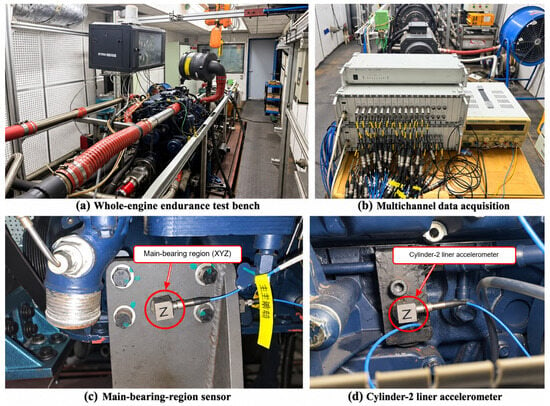
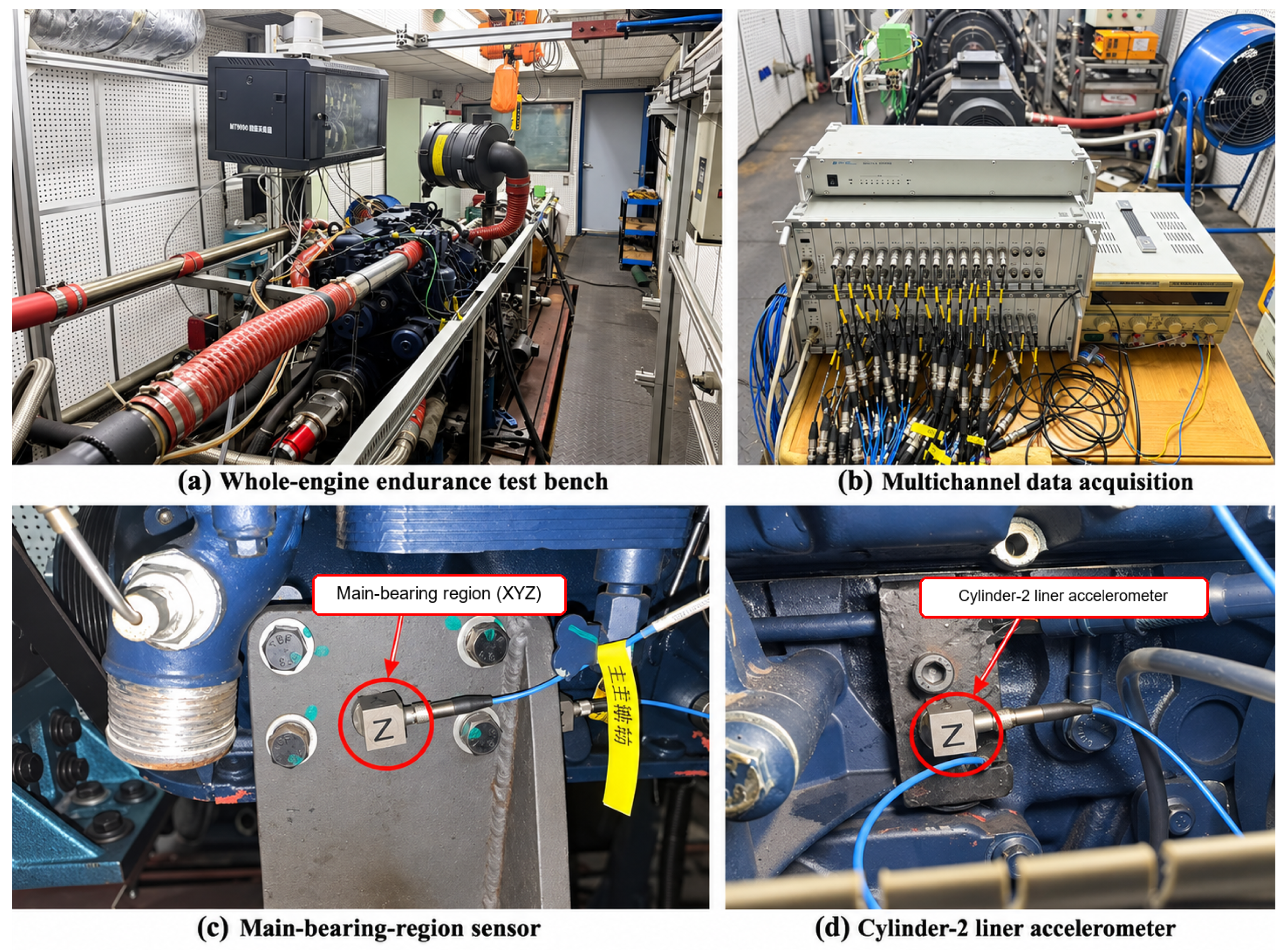
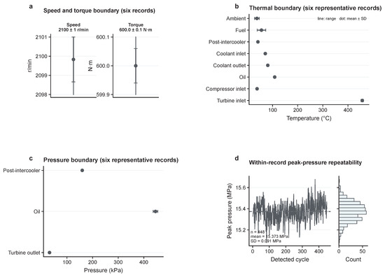
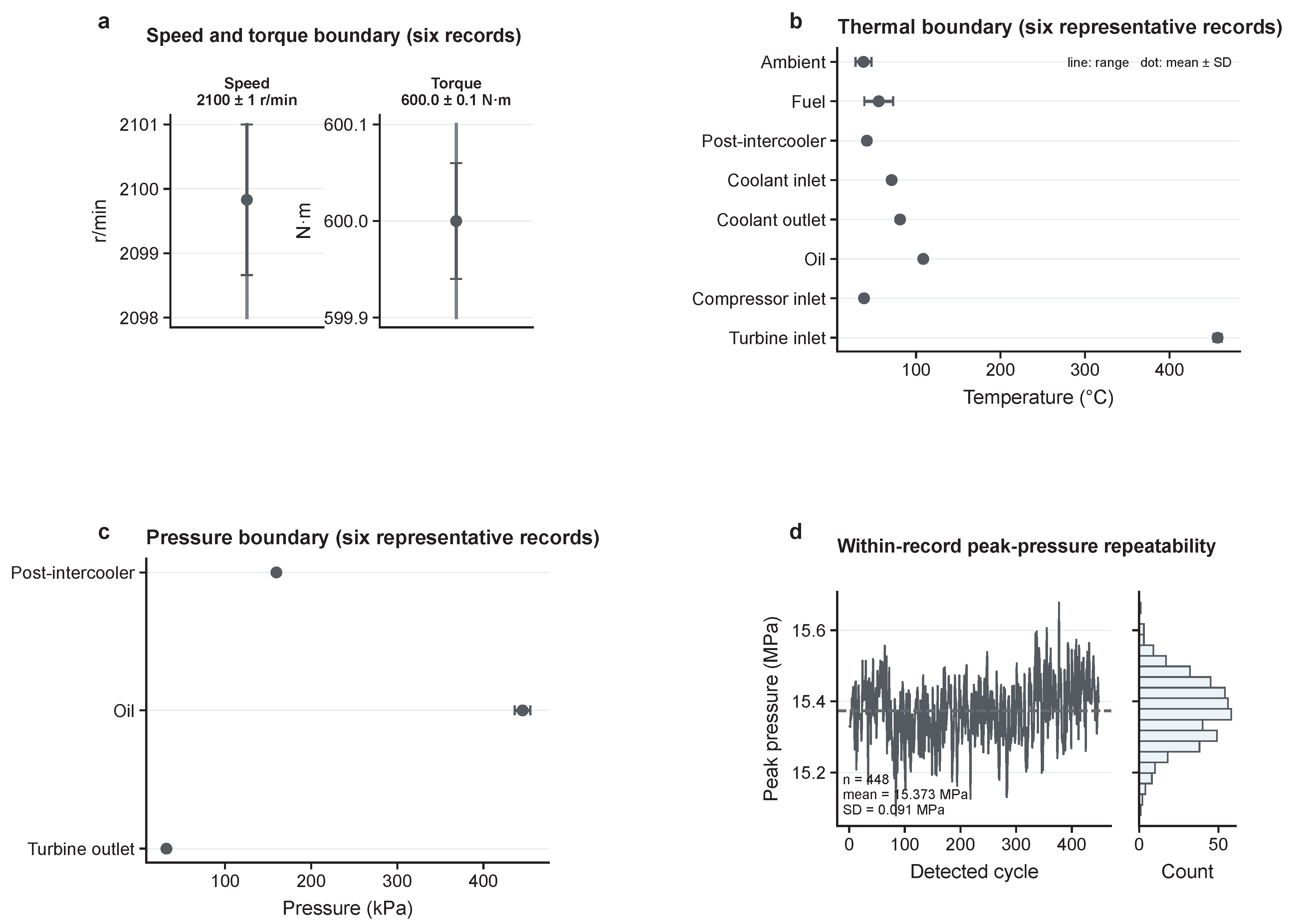
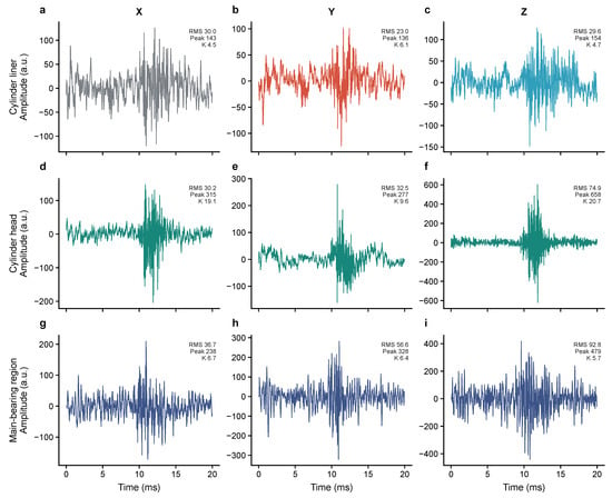
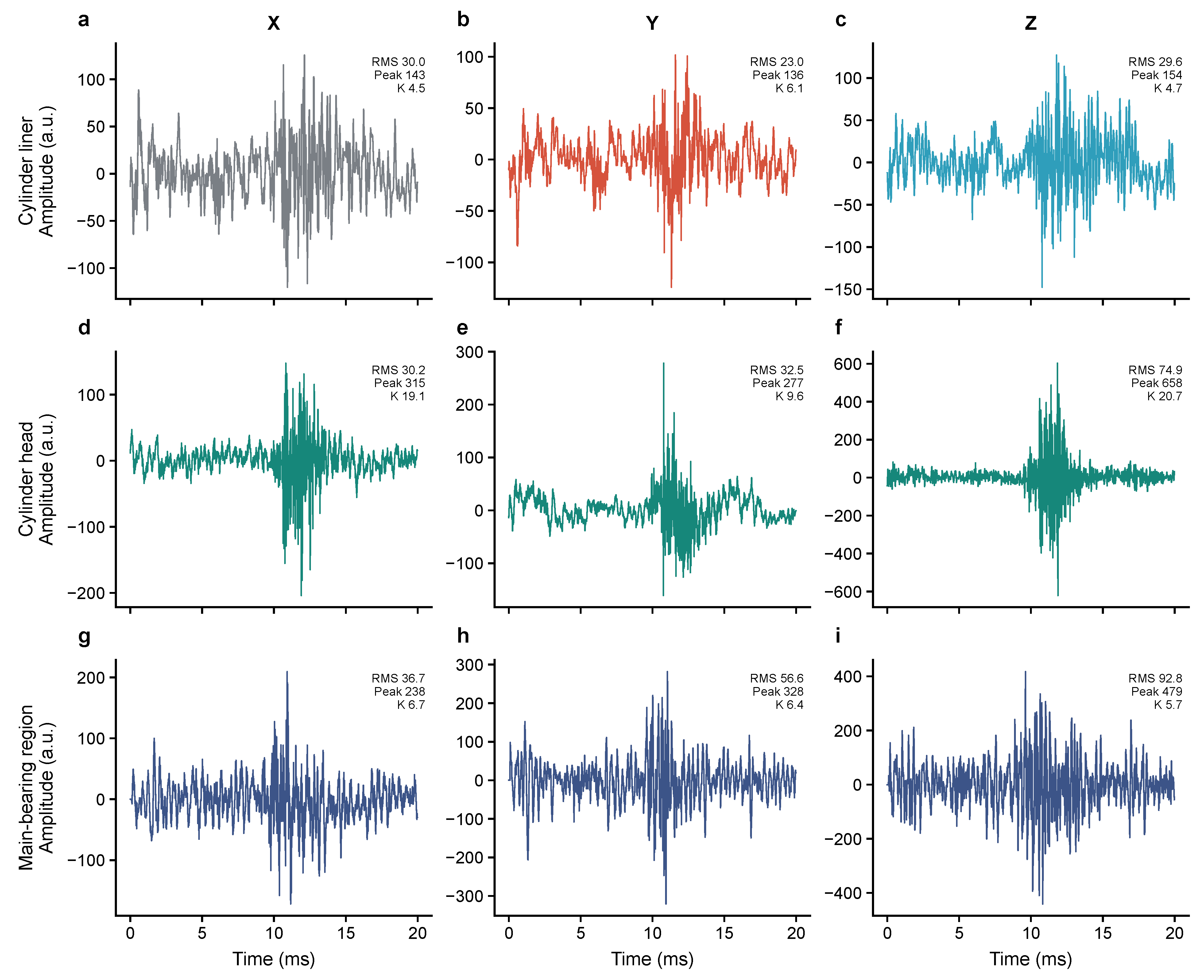
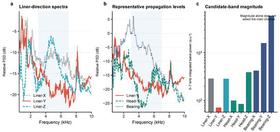
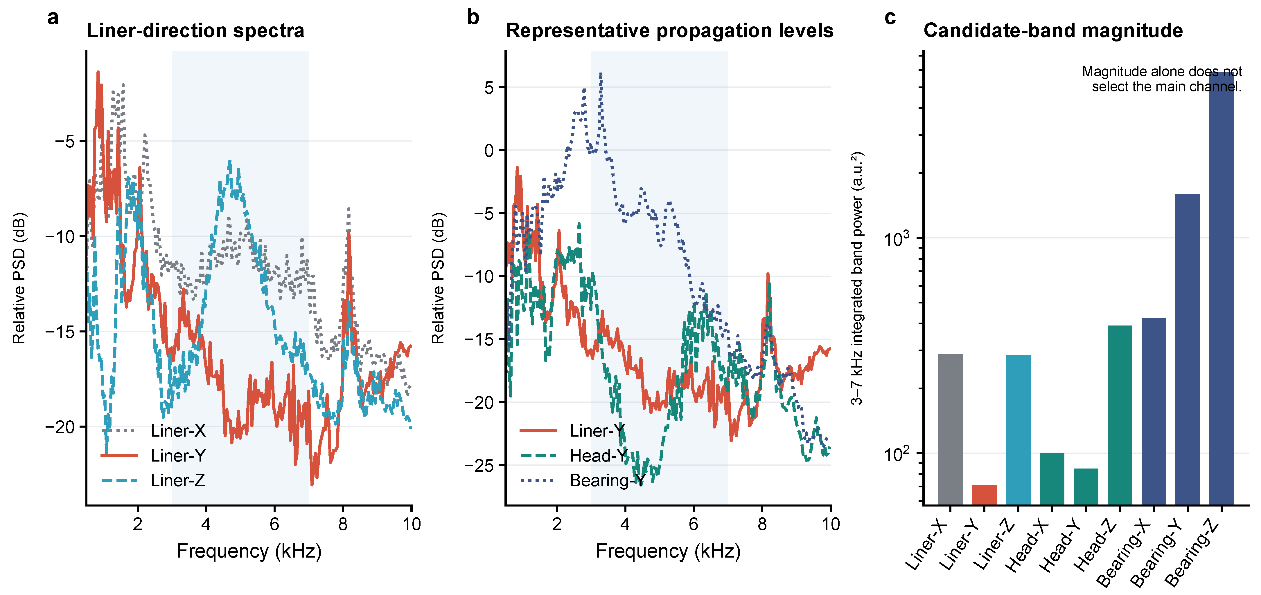
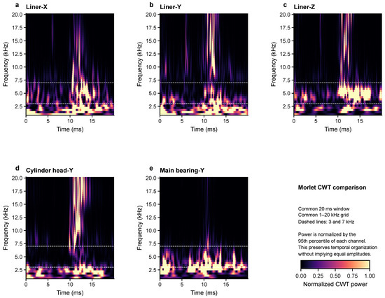
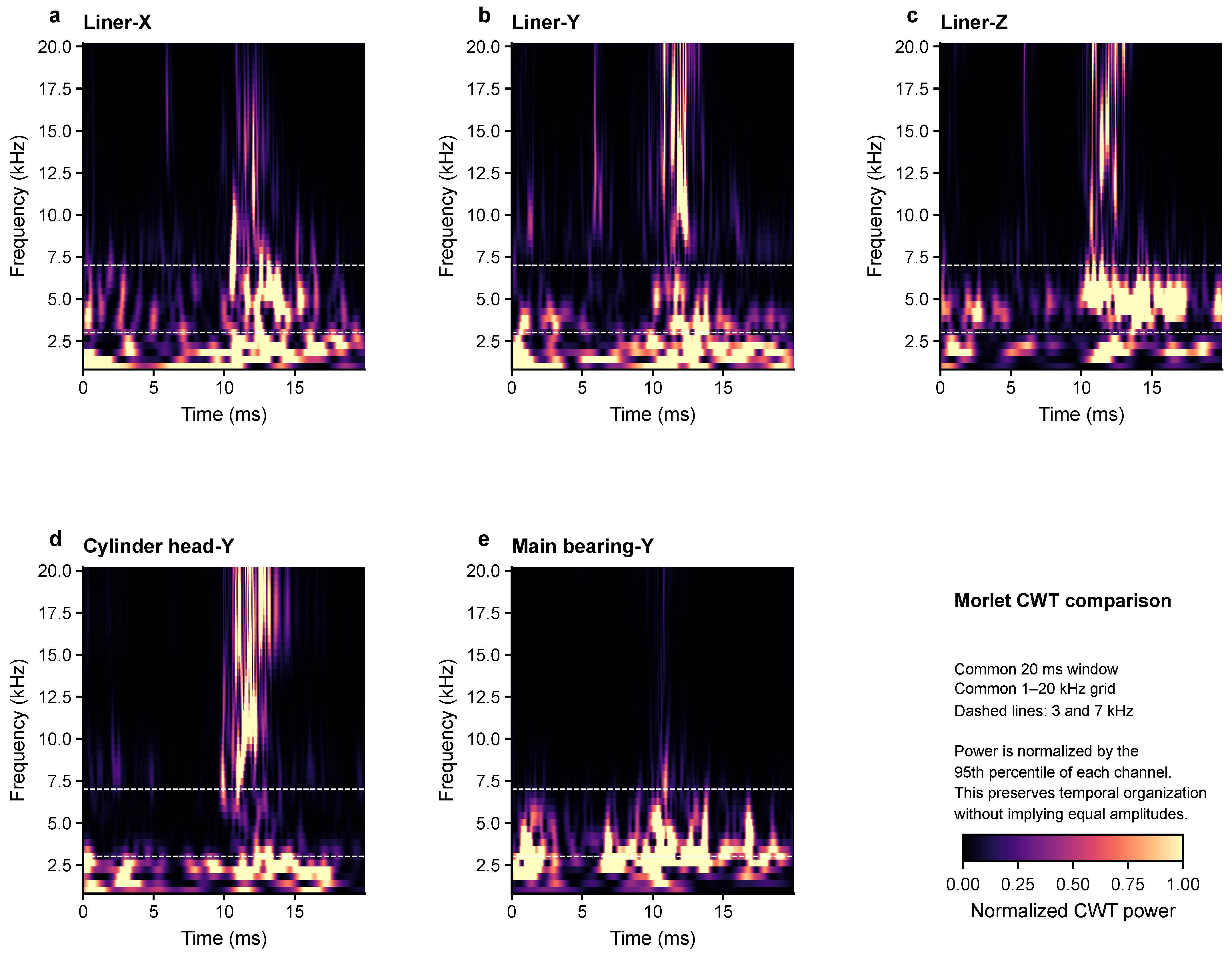
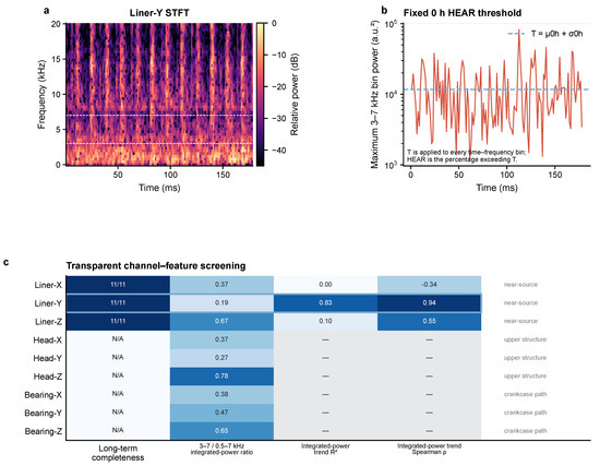
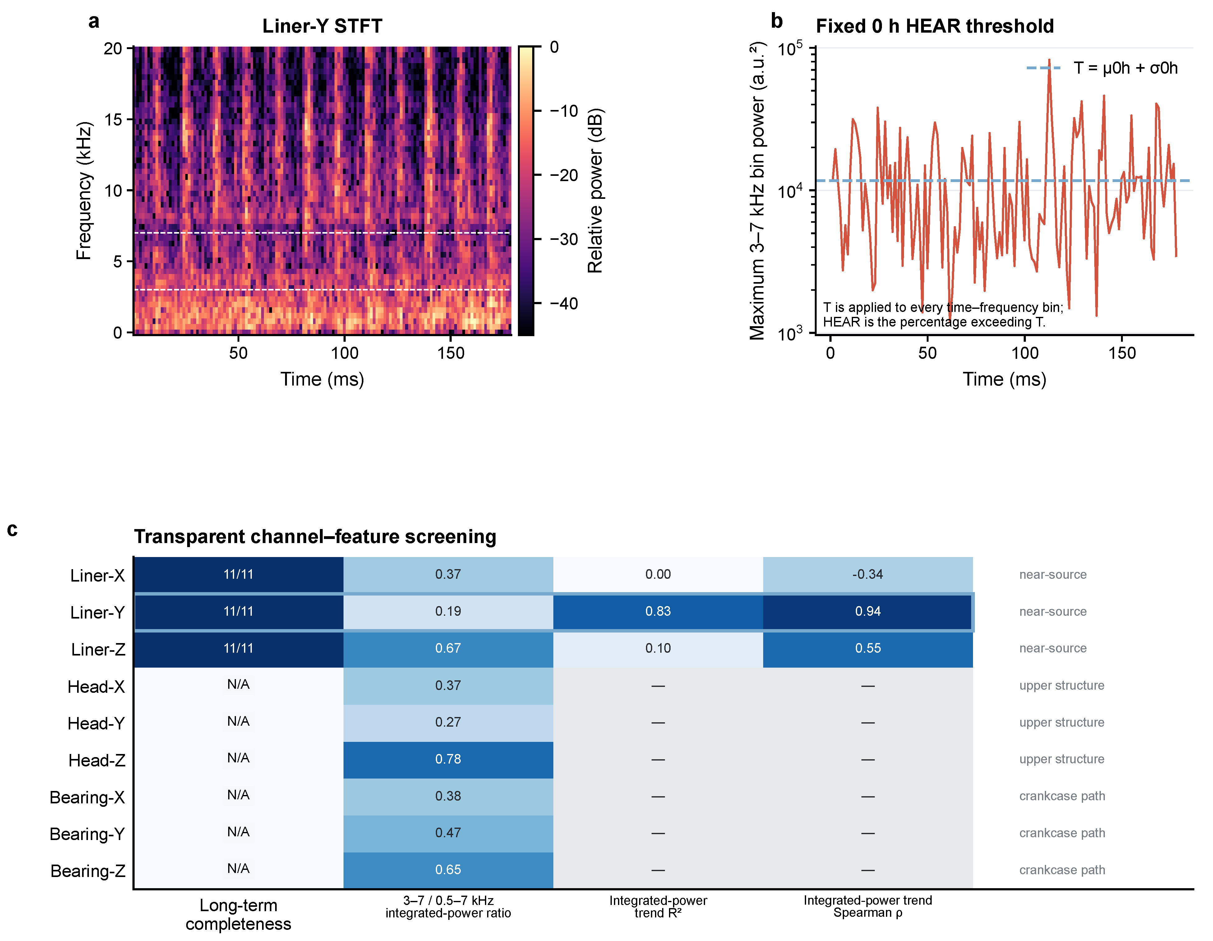
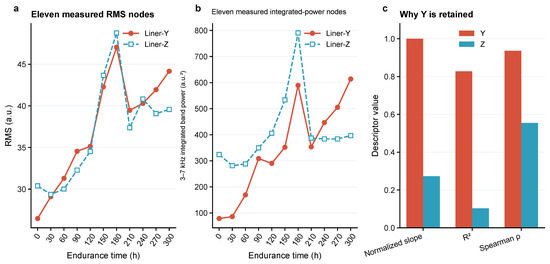
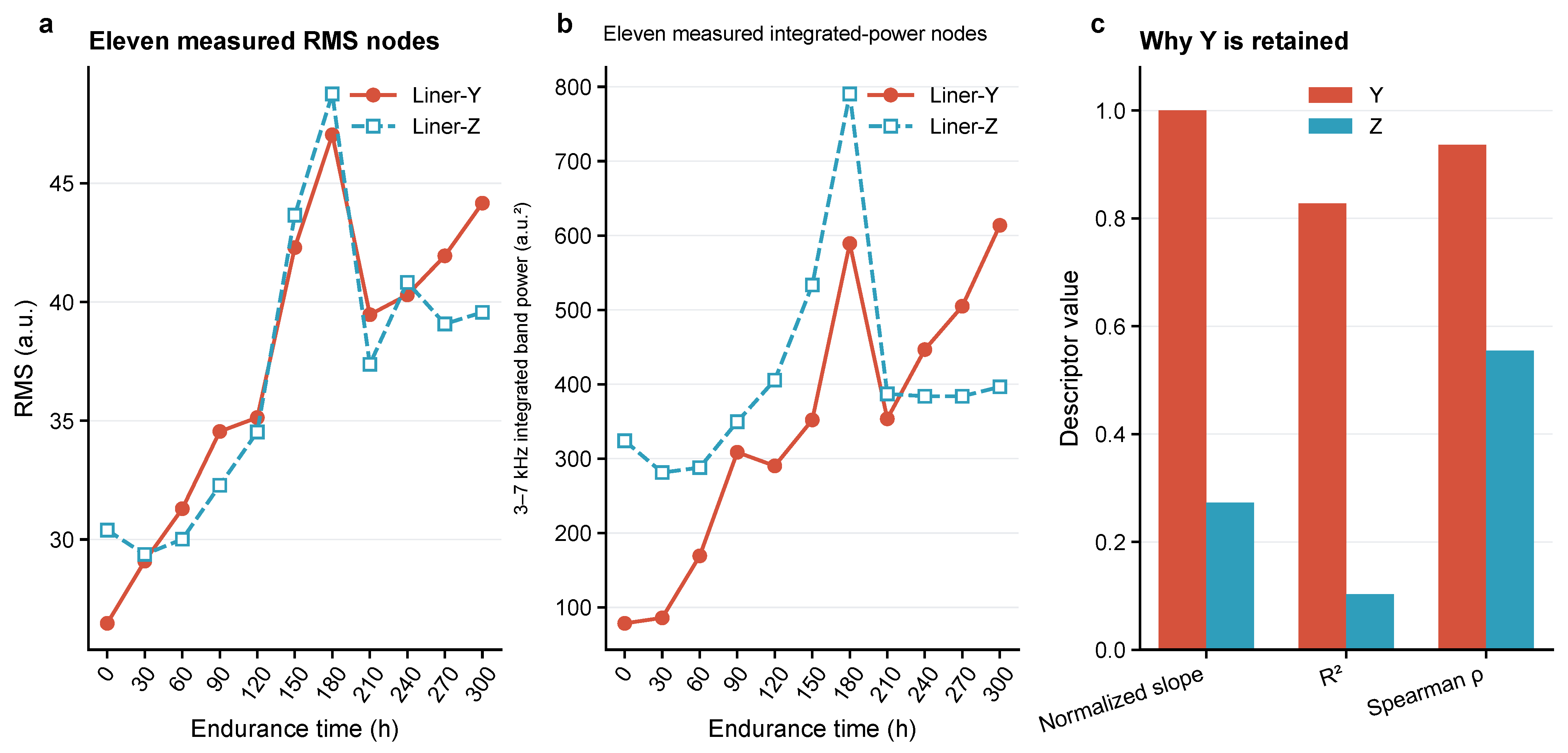
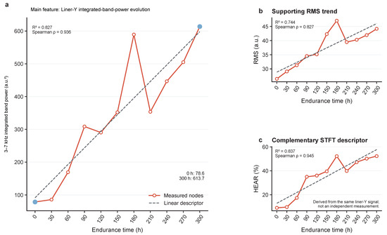
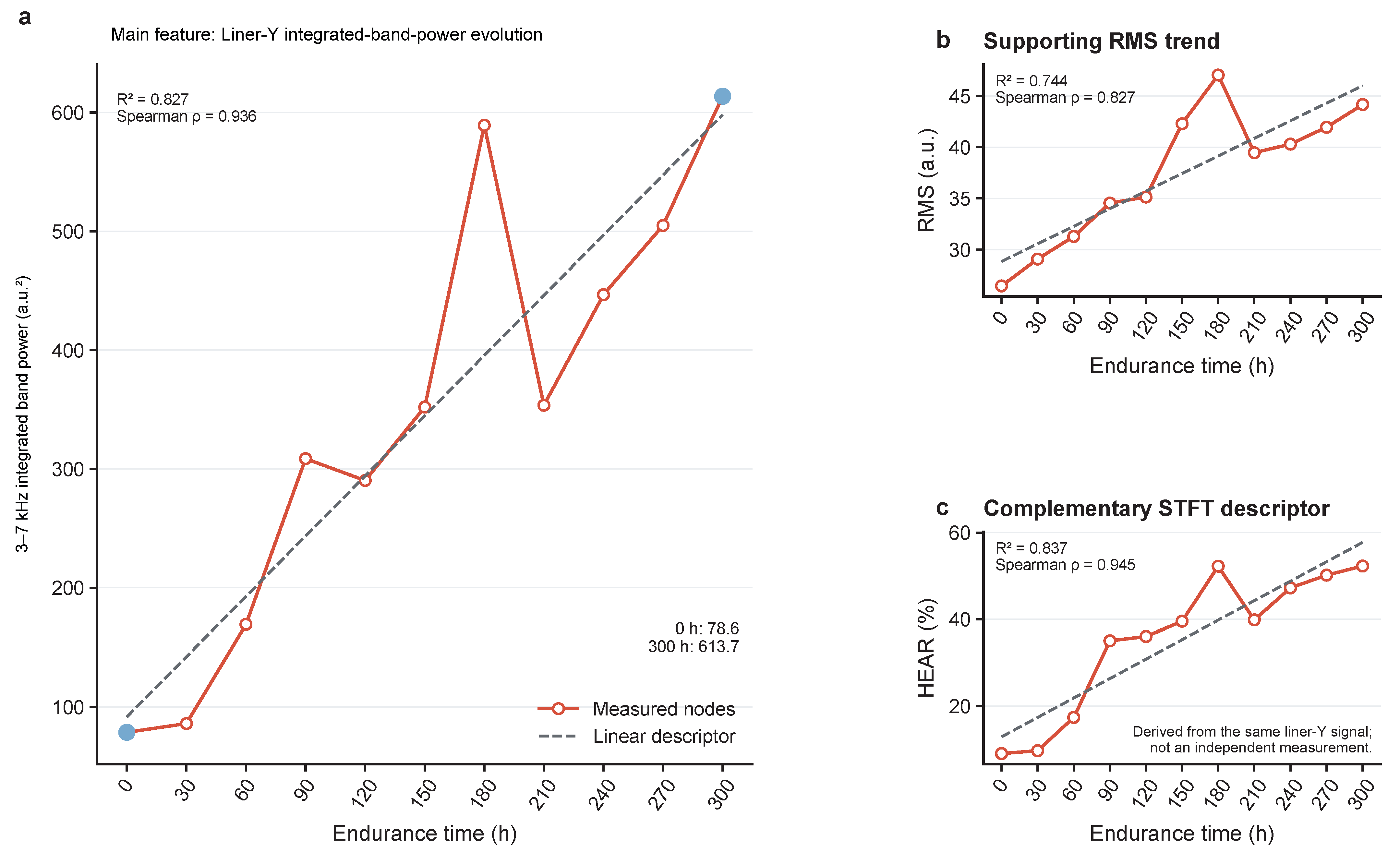
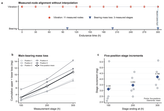
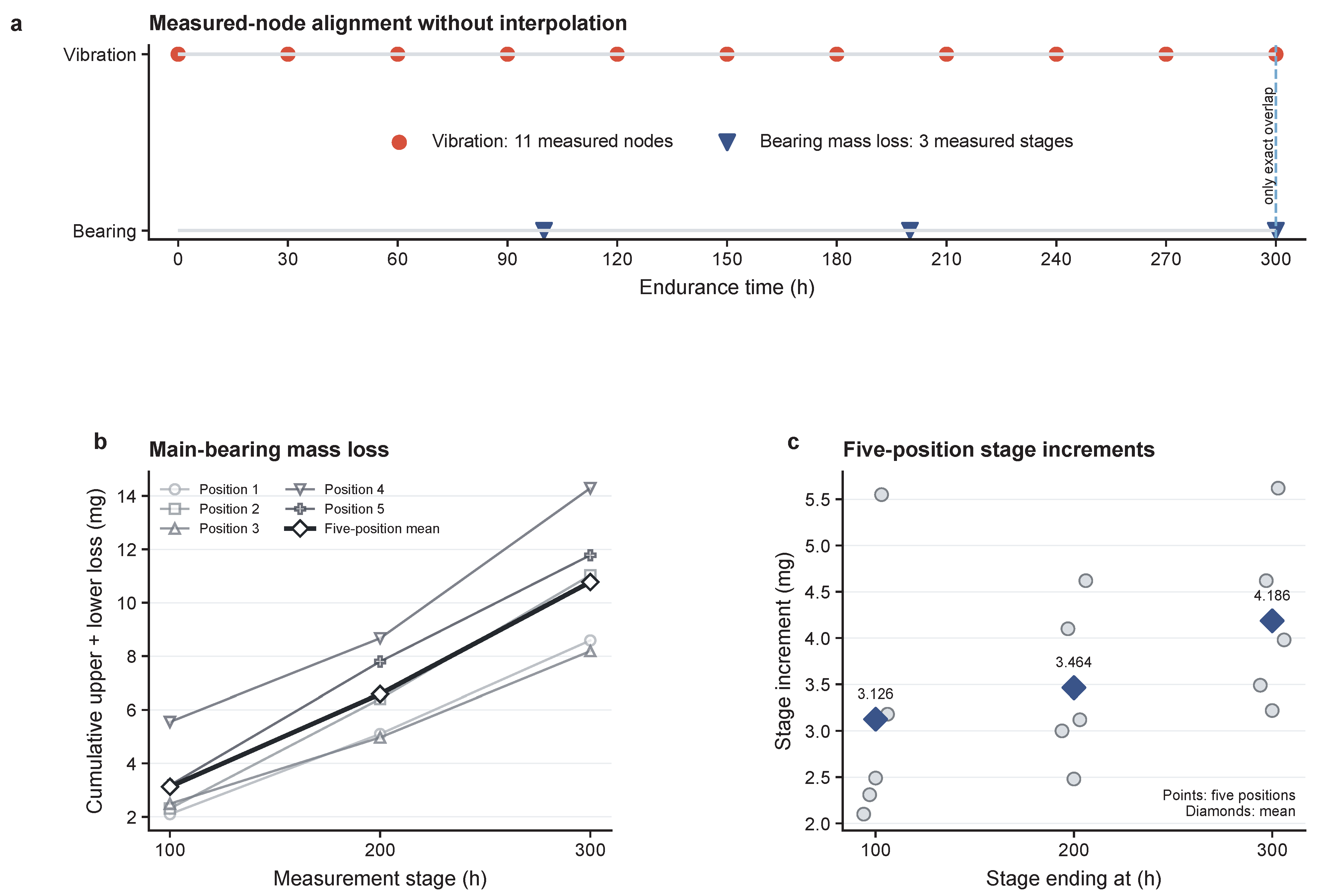
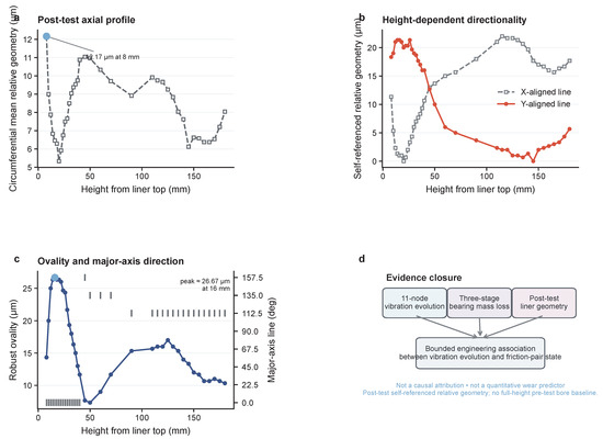
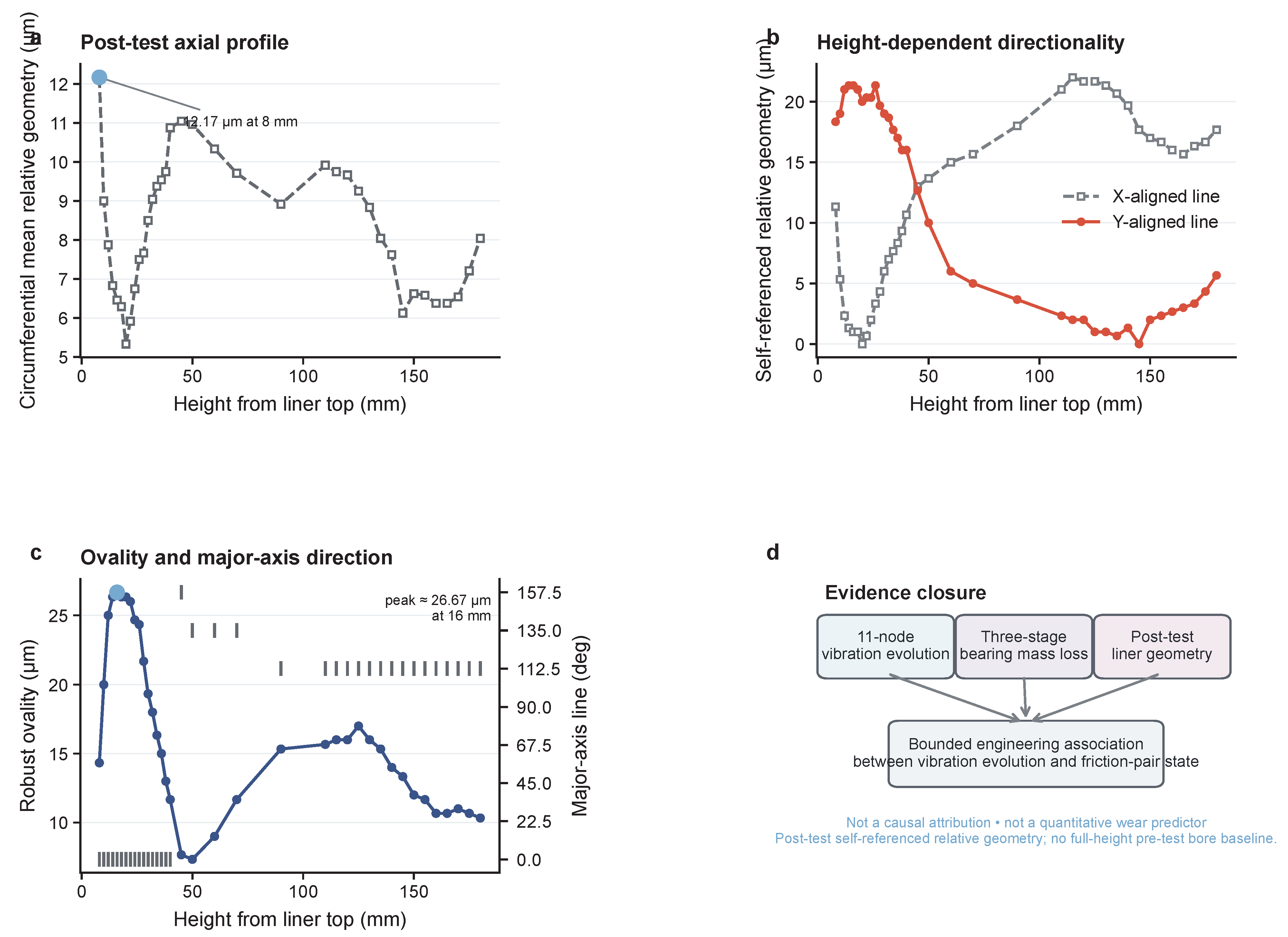

Disclaimer/Publisher’s Note: The statements, opinions and data contained in all publications are solely those of the individual author(s) and contributor(s) and not of MDPI and/or the editor(s). MDPI and/or the editor(s) disclaim responsibility for any injury to people or property resulting from any ideas, methods, instructions or products referred to in the content. |
© 2026 by the authors. Licensee MDPI, Basel, Switzerland. This article is an open access article distributed under the terms and conditions of the Creative Commons Attribution (CC BY) license.