


Abstract
In large-scale stochastic many-objective time–cost–environment trade-off problems, influence is unevenly distributed: each objective is governed by a reduced subset of the decision variables that drive most of the controllable variation, while the remaining variables enlarge the Pareto search space—and the set of levers managers must deliberate over—without materially affecting performance. This study integrates Monte Carlo simulation, surrogate modeling, Sobol global sensitivity analysis, and many-objective evolutionary optimization to identify that influential subspace and confine the search to it, demonstrated on a 30-task construction project with 68 input variables, five conflicting objectives, and 150,000 training scenarios. Multi-criteria benchmarking of eleven surrogate architectures and eight evolutionary algorithms selected a Multilayer Perceptron (R2 = 0.993, MAE = 3.962 × 10⁻³) and AGE-MOEA (HV = 0.741, IGD = 0.064, SP = 0.036). Sobol screening reduced the decision space from 60 to 40 task-interpretable variables; at equal budget, the reduced space retains 91.6–95.5% of the full-space hypervolume, a front-level cost that exceeds the discarded sensitivity mass (0.3–2.2%) and quantifies, for this instance, the behaviour of the Factor Fixing criterion at the front level. A space budget analysis showed that both spaces converge well before the full budget (2.0–2.2× speedup at no more than 1.7% additional hypervolume loss): the efficiency gain stems from the budget, while the screening contribution is structural: it identifies which scheduling decisions can be fixed at nominal values, at the cost measured above. An a posteriori re-evaluation with the exact model bounded the optimistic surrogate error (MAPE 1.26–4.38%; 118 of 126 solutions feasible), and the CRITIC-weighted selection yielded a 36.46-day schedule at USD 283,189 with a sustainability index of 0.924.
1. Introduction
Project management has evolved beyond a purely administrative discipline into a domain of complex optimization, seeking to balance economic efficiency, sustainability, and human well-being [1]. Recent literature emphasizes that the success of modern industrial projects hinges on the ability to manage multiple conflicting objectives simultaneously, including cost minimization, schedule adherence, and environmental impact reduction [2,3].
Within this framework, stochastic many-objective time-cost-environment trade-off problems with precedence constraints constitute a class of challenges for which traditional solution approaches often prove inadequate, owing to the dynamic and stochastic nature of industrial variables, as well as their inherently large scale [4]. Building on the classical time-cost trade-off problem, a long-standing line of work models activity cost as a convex function of its duration [5,6,7], reflecting the diminishing returns of schedule acceleration documented empirically for extended overtime in construction [8,9]. Multi-mode extensions further associate discrete execution modes with distinct cost premiums and environmental intensities [10,11], giving rise to time-cost-environment formulations in which cleaner technologies reduce energy, water, and carbon intensity at a bounded additional cost [12,13,14]. Uncertainty enters these problems through two complementary channels: the wide, distribution-dependent variability of task durations and unit rates documented across construction projects—empirical analyses of over 5000 activities report only weak-to-moderate correlations (R2 = 0.10 − 0.62) between duration and cost deviations, with variability arising from largely distinct sources [15,16]—and the parametric uncertainty of the environmental response itself, conversion factors and non-linear scaling exponents that vary with site conditions and technology [17]. Stochastic formulations that account for these sources of uncertainty therefore provide a more faithful representation of modern project environments than their deterministic counterparts [3,18].
As project scheduling environments grow in complexity, modern time-cost-environment trade-off problems increasingly involve more than 50 decision variables, a characteristic known as large-scale optimization, while simultaneously exceeding three conflicting objectives, a classification known as Many-Objective Optimization Problems (MaOPs) [19]. The concurrent presence of both properties defines a large-scale MaOP, posing significant computational challenges for conventional optimization frameworks.
When these problems additionally incorporate stochastic parameters, they constitute a subclass known as stochastic many-objective project scheduling problems [17]. Contemporary formulations of this subclass further extend the objective space to include environmental sustainability criteria [3,20], significantly expanding both the decision and objective spaces.
The high dimensionality of the decision space introduces a twofold challenge in large-scale project scheduling. Computationally, the growth of the search domain enlarges the region the search must cover and, where evaluation cost scales with dimension, the cost per optimization run [21]. Managerially, it multiplies the number of levers a decision-maker must deliberate over. In such settings, however, influence is typically concentrated: for each objective, a reduced subset of the decision variables governs most of the controllable variation in project outcomes, and even after consolidating these subsets across all objectives, part of the decision space enlarges the search domain—and the deliberation burden—without materially affecting performance [21,22]. This motivates the development of systematic variable screening frameworks with a dual purpose: to confine the Pareto-based search to the subspace that demonstrably drives performance, and to estimate, at a quantified cost, which decisions may be fixed at nominal values so that decision effort concentrates on the variables that matter.
To mitigate the computational cost of evaluating many-objective project scheduling problems, recent literature has championed the use of surrogate models or metamodels, such as artificial neural networks or random forests, to approximate the fitness landscape. However, a significant gap remains in the methodological treatment of the input domain. To address this, the literature identifies two primary pathways for dimensionality reduction: unsupervised and supervised techniques [23].
Unsupervised techniques, such as Principal Component Analysis or Autoencoders, focus on feature extraction, transforming the original variables into a lower-dimensional latent space to capture maximum variance or topological structures without considering the target objectives [24]. While efficient for data compression, these methods often sacrifice the interpretability of the original project tasks. Conversely, supervised techniques, such as Linear Discriminant Analysis or variance-based feature selection, leverage the relationship between inputs and outputs to identify the most relevant variables [22,25].
Despite the proven efficacy of Global Sensitivity Analysis (GSA) as a supervised reduction framework in complex engineering based on variance decomposition, its application as a systematic pre-processing step for variable screening in large-scale project scheduling remains underexplored [1,26]. Current scheduling frameworks typically assume that all decision variables must be optimized with equal weight, overlooking the potential of a sensitivity-based reduced space.
Among GSA methods, variance-based decomposition approaches, such as Sobol, Sobol-Jansen, or Sobol2007, stand out for their ability to quantify the propagation of input uncertainty to model outcomes and to identify both individual and interaction effects among variables [22,27]. Variance-based GSA methods have seen widespread adoption in the analysis of complex systems [28]. However, a significant limitation of variance-based GSA is its reliance on extensive Monte Carlo sampling, which often requires a prohibitive number of model evaluations for large-scale scenarios.
To mitigate this computational burden, surrogate models or metamodels have been proposed as computationally efficient approximations of the original fitness landscape. These metamodels, commonly constructed using machine learning approaches, enable large-scale sampling required for sensitivity decomposition while substantially reducing overhead associated with the original simulation [29]. By leveraging resulting sensitivity indices, it becomes possible to identify and isolate the reduced decision subspace of the problem, concentrating optimization efforts on the variables that predominantly govern system performance.
In this context, we hypothesize that the Sobol method enables the identification of a reduced decision subspace within the high-dimensional decision space of stochastic many-objective time-cost-environment trade-off problems, such that optimization within this reduced space achieves competitive Pareto front quality relative to the full decision space, as measured by hypervolume, inverted generational distance, and spacing, at a quality cost that is bounded and empirically quantified, while preserving the task-level interpretability of the scheduling decisions.
To validate this hypothesis, this study integrates surrogate modeling with the Sobol method to determine the reduced decision subspace and facilitate the search for optimal solutions. We first establish a robust computational design of experiments using Latin-hypercube sampling, which improves marginal stratification and coverage of the high-dimensional input domain. This sampling facilitates systematic stochastic project simulations to compute fitness across five objectives, generating the comprehensive datasets required for multi-target validation. Leveraging this data, we construct high-fidelity metamodels through machine learning architectures to approximate the fitness landscape with minimal computational overhead. These models serve as the substrate for identifying the most influential decision variables via the Sobol method, condensing the problem dimensionality into a reduced decision subspace. The resulting reduced-space problem is then solved by deploying many-objective evolutionary algorithms, with the uncontrollable stochastic parameters held at their mean values: uncertainty is thus characterized and propagated upstream of the search, which is conducted under nominal environmental conditions, so that the identified Pareto front is conditional on those conditions.
This research advances large-scale project scheduling through three primary contributions:
- We introduce a supervised dimensionality reduction framework grounded in Sobol-driven GSA. Unlike unsupervised methods such as PCA, which transform variables into abstract components, this approach isolates a reduced decision subspace that preserves the interpretability of project tasks and estimates the cost, in attainable front quality, of fixing the screened-out decision variables at nominal values. This bridges a critical gap in high-dimensional project scheduling [1,23,24,26,30], where systematic filtering of non-influential variables remains largely underexplored.
- We establish a robust surrogate benchmarking architecture that transcends the traditional trial-and-error hyperparameter tuning prevalent in project scheduling literature, a methodology gap explicitly highlighted in a recent systematic review [30]. By deploying a successive-halving grid search for the automated optimization of eleven machine learning models, we ensure an efficient exploration of the configuration space. The optimal surrogate selection is formalized through Multi-Criteria Decision Making (MCDM), integrating R2, MAE, RMSE, and MSE as evaluation criteria.
- We provide a comprehensive benchmarking of eight evolutionary algorithms within the identified reduced decision space. While conventional studies often rely on a single performance metric, predominantly hypervolume [4,26], our framework formalizes algorithm selection via MCDM by integrating hypervolume, inverted generational distance, and spacing as evaluation criteria, ensuring a simultaneous assessment of convergence, diversity, and solution distribution, complemented by a space budget analysis that disentangles the contribution of the subspace from that of the optimization budget.
The remainder of this work is structured as follows. Section 2 (Materials and Methods) details the theoretical foundations and the five-stage methodology designed to integrate dimensionality reduction into many-objective optimization problems. Section 3 (Results and Discussion) presents the empirical findings derived from applying this framework to a high-dimensional stochastic project scheduling instance, characterized by sixty-eight input variables and five objective functions, complemented by an a posteriori sustainability index. This section further contextualizes the performance of the surrogate models and evolutionary algorithms within the identified reduced decision subspace. Finally, Section 4 (Conclusions) summarizes the primary scientific contributions, outlines the practical implications and proposes directions for future research in large-scale optimization.
2. Materials and Methods
This section presents the theoretical framework and computational methodologies employed in this study. It details a five-stage framework that integrates surrogate modeling, global sensitivity analysis, and many-objective evolutionary optimization to address the stochastic many-objective time-cost-environment trade-off problem.
2.1. Many-Objective Evolutionary Algorithms
Many-objective optimization problems (MaOPs) involve four or more conflicting objectives, posing significant challenges for classical Pareto-based algorithms. As the number of objectives increases, these algorithms often struggle with a diminished selection pressure toward the Pareto front [19]. To address these challenges, many-objective evolutionary algorithms (MaOEAs) have been developed as specialized tools. Recent advances have expanded their application in engineering and scheduling domains [31,32]. Consequently, a selection of state-of-the-art MaOEAs was adopted for this study. Additionally, several well-established multi-objective algorithms (R-NSGA-II, SPEA2, and NSGA-II) were included to serve as benchmarks for performance and scalability comparisons.
- NSGA-III (Non-Dominated Sorting Genetic Algorithm III): An extension of NSGA-II that replaces the crowding distance mechanism with a niche strategy based on a set of widely distributed reference points, generated via the Das-Dennis simplex-lattice design and used to associate solutions with the nearest reference direction, thereby preserving diversity in high-dimensional objective spaces [33,34].
- AGE-MOEA (Adaptive Geometry Estimation-based MOEA): This algorithm adapts its survival selection mechanism to the local geometry of the Pareto front. This allows for robust performance across convex and irregular objective landscapes without requiring predefined reference vectors [35].
- RVEA (Reference Vector-Guided Evolutionary Algorithm): It employs an angle-penalized distance (APD) metric that guides selection toward the reference vectors. It includes an adaptive strategy for updating the reference vectors to manage the evolving shape of the Pareto front. It is included in this study as a specialized many-objective benchmark [36].
- SMS-EMOA (S-Metric Selection EMOA): A steady-state algorithm that, at each iteration, removes the individual contributing the least to the hypervolume (S-metric) [37]. Its theoretical runtime properties in many-objective settings are well-characterized in the literature [38].
- MOEA/D (Multi-objective evolutionary algorithm based on decomposition): This approach transforms a many-objective problem into a set of scalar subproblems using Tchebycheff decomposition (or scaling), optimizing them simultaneously through neighborhood interactions [39].
- R-NSGA-II (Reference-based NSGA-II): An algorithm designed to search for specific regions within the objective space based on user-defined preferences. It utilizes target-level reference points and an ε-clearing mechanism [40].
- SPEA2 (Strength Pareto Evolutionary Algorithm): It employs a fine-grained fitness assignment based on Pareto dominance, nearest-neighbor density estimator, and an archive pruning procedure that preserves boundary solutions [41].
- NSGA-II (Non-dominated Sorting Genetic Algorithm II): Although not originally designed for many-objective scalability, its mechanism, based on crowding distance, serves as the primary benchmark to evaluate the performance gains of specialized MaOEAs against a well-established standard [42].
2.2. Machine Learning (ML)
ML is a specialized field of artificial intelligence focused on developing algorithms that allow computers to learn from and make predictions on data without being explicitly programmed for every specific task. Rather than following static instructions, ML models identify underlying patterns and relationships within datasets to improve their performance autonomously over time. ML approaches can address both supervised and unsupervised learning tasks. The former includes regression and classification problems. Specifically, when regression is used to approximate complex simulation data, the resulting model is referred to as a surrogate model. These models act as data-driven approximations that emulate computationally expensive simulations, aiming to provide accurate results at a fraction of the original computational cost [43,44]. For instance, they are frequently employed to accelerate the execution of GSA.
A wide array of ML regression models can be employed as surrogates [45,46]. Common examples include linear models such as ElasticNet (EN) and Ridge regression (R); non-parametric methods like K-Nearest Neighbors (KNN) and ensemble-based techniques such as Random Forest (RF), Extra Trees (ET), Bagging (BA), AdaBoost (AB), Gradient Boosting (GB), XGBoost (XGB), and Histogram-based Gradient Boosting (HGB). Additionally, connectionist approaches like the Multilayer Perceptron (MLP) are frequently used. The performance of these models is highly sensitive to their hyperparameters, as well as the quality and size of the training dataset, among other critical factors. Despite their versatility, these models are not typically compared within the context of stochastic many-objective project scheduling; therefore, conducting a comprehensive performance evaluation of these surrogates constitutes one of the primary contributions of this work.
2.3. Global Sensitivity Analysis (GSA)
GSA is a methodological approach grounded in variance-based techniques, which quantifies the contribution of each input variable to the output variance. This is achieved by decomposing the total variance of a model output, denoted as V(Y), into components attributable to individual inputs and their interactions across the entire factor space [47]. Among the various methodologies available for such decomposition, the Sobol method stands as the benchmark approach.
The procedure requires the construction of independent sampling matrices (A and B) of size N × k where N is the number of samples and k the number of input variables. To isolate the effect of a specific variable i, a hybrid matrix is created by substituting the i − th column of A with the i − th column of B. The mathematical model, defined as Y = f(X), is then evaluated for all matrices, yielding output vectors YA = f(A), YB = f(B), and [27]. For each input variable Xi, two sensitivity indices are calculated:
Here, S1,i represents the first-order sensitivity index, which quantifies the direct contribution of Xi to the output variance. Conversely, ST,i is the total-order sensitivity index, which captures the direct effect of Xi plus all higher-order interaction effects involving that variable. In these expressions, E(∙) is the expected value, and X~i refers to the set of all input variables except Xi.
2.4. Multi-Criteria Decision Making (MCDM)
MCDM provides a structured framework for ranking a finite set of alternatives evaluated against multiple, often conflicting criteria. In this study, as will be described in the Section 2.5, these methods are used to determine the best ML model, as well as the best optimization algorithm. These methods can be found in [48,49]:
- TOPSIS (Technique for Order Preference by Similarity to Ideal Solution): This method ranks alternatives based on their geometric distance from both the ideal and anti-ideal solutions. An alternative is prioritized if it is simultaneously closest to the ideal solution and farthest from the anti-ideal one, determined by a closeness coefficient.
- MOORA (Multi-Objective Optimization by Ratio Analysis): This approach utilizes ratio-based normalization to render criteria comparable across different scales. A final scalar score is derived from the difference between the weighted sums of beneficial criteria (to be maximized) and non-beneficial criteria (to be minimized).
- SAW (Simple Additive Weighting): As one of the most widely implemented MCDM methods, SAW computes a weighted linear combination of the normalized criterion values. This yields a single utility score that represents the overall performance of each alternative.
- WASPAS (Weighted Aggregated Sum-Product Assessment): This technique enhances decision-making robustness by integrating the weighted sum model (WSM/SAW) with the weighted product model (WPM). By balancing additive and multiplicative aggregations through a joint criterion, it provides more stable rankings.
- ARAS (Additive Ratio Assessment): This method establishes an optimal reference alternative as a benchmark. Candidates are then ranked according to the ratio between their weighted performance sum and that of the reference alternative, effectively measuring how close each candidate is to the theoretical optimum.
2.5. Methodology
This section details the methodology adopted to conduct this research, the core stages of which are visually summarized in Figure 1.
Figure 1.
Systematic overview of the surrogate-assisted optimization and decision-making process for the stochastic many-objective optimization problem.
2.5.1. Computational Design of Experiments (CDoE)
The study is based on a construction project comprising 30 interdependent tasks, where each task is characterized by two decision variables: its execution duration and its technology mode. The project therefore involves 68 input variables (60 decision variables—30 continuous durations and 30 ordinal technology modes—and 8 stochastic parameters, Table 1), and five conflicting objectives (time, cost, energy, water, and greenhouse-gas emissions). A sustainability index is derived a posteriori for decision-making and is not part of the optimization problem. The problem is formulated as a stochastic many-objective time-cost-environment trade-off problem with precedence constraints, distinct from a resource-constrained project scheduling problem in that no resource-capacity constraints are imposed. Feasibility is governed solely by precedence relations among tasks and by operational bounds on the decision variables (Section 2.5.5).
Table 1.
Experimental design configuration: calibration families, assignment rule, task counts, and parametric settings for task durations and stochastic parameters.
The 60 decision variables comprise two controllable scheduling parameters per task—its execution duration and its technology mode—which are directly optimized within the many-objective framework. The cost rate of a task is not an independent decision but is derived from this pair through the compression function of Equation (1), consistent with standard time-cost trade-off formulations. Activity start times follow from the durations through critical-path-method logic, which enforces all precedence relationships among the 30 tasks. The precedence network was generated once at random—each task after the first drawing one or two predecessors uniformly among lower-indexed tasks under a fixed seed—and held fixed throughout the study. The optimizer searches over the feasible ranges of these pairs to identify Pareto-optimal schedules, and the resulting solutions are directly interpretable as scheduling decisions.
The remaining 8 input variables are uncontrollable stochastic parameters: the energy conversion factor (αE), water conversion factor (αW), greenhouse gas emission factor (βCO2), energy allocation fraction (ϕE), water allocation fraction (ϕW), and the non-linear exponents (γE, γW, δ). They are treated as stochastic inputs within the CDoE framework, sampled via Monte Carlo simulation during the CDoE stage to characterize uncertainty in the objective function space, and subsequently held at their mean values during optimization. The Pareto front therefore reflects structural trade-offs among scheduling objectives under nominal environmental conditions, rather than favorable combinations of uncertainty parameters.
Under deterministic conditions, the project baseline is characterized by an execution time of 52.64 days and a total investment of 209,990 USD. Furthermore, the associated resource demand includes an energy requirement of 24,888 kWh, water consumption of 455.02 m3 and a carbon footprint of 4555 kg CO2-eq.
To evaluate the impact of variability on project outcomes, a CDoE was implemented using Monte Carlo simulation with 150,000 Latin-hypercube sampling points, which improve marginal stratification and coverage of the 68-dimensional input domain. This approach stratifies the marginal distribution of each input but does not guarantee uniform joint coverage in 68 dimensions; the coverage actually achieved over the reachable decision space is therefore assessed empirically in Section 3, where the design is shown to span 81% of the attainable makespan range. The nominal duration and cost rate of each task were set as the analytical median of its calibration family (Table 1), scaled by the square root of a task-size factor drawn once per task under a fixed seed from a log-normal distribution (σ = 0.9, unit mean). This reproduces realistic size heterogeneity, with a few tasks concentrating most of the work content. Each duration ranges from half to 1.7 times its nominal value, with a one-day floor. Within the CDoE, durations were sampled over these ranges by combining a scenario-level compression factor (weight 0.25), shared by all tasks so that coherently compressed schedules are represented in the training set, with task-specific uniform draws; this shared factor is a sampling device, not a surrogate input. Technology modes were sampled uniformly over their three levels, and the stochastic parameters from the normal distributions of Table 1.
These distributions play two complementary roles. For the 60 controllable scheduling variables, the families in Table 1 play a calibration role: their analytical medians provide the family-level baselines from which the nominal durations and cost rates of Equations (1) and (2) are constructed after task-size scaling, as described above. These sampled values do not represent irreducible uncertainty, since they are ultimately selected by the optimizer. In contrast, the distributions of the 8 stochastic parameters describe genuinely uncontrollable variability; these parameters are propagated through the simulation and subsequently held at their mean values during optimization.
The distribution families in Table 1 were selected to reflect realistic construction variability: bounded distributions (triangular and uniform) capture duration and cost uncertainty within practical operational ranges, log-normal distributions model right-skewed resource peaks while preventing non-physical negative values, and normal distributions govern global conversion and non-linear parameters consistent with industrialized processes.
2.5.2. Project Simulation and Metrics
The project outcomes were derived through an integrated physical-economic model. Following the convex (non-linear) time-cost trade-off tradition [5,6,7,15], the cost rate of each task is a compression function of its duration and technology mode:
where and are the nominal cost rate and duration of task t (calibrated as described in Section 2.5.1), κt is the task-specific crashing elasticity, and a is the maximum cost premium of the cleanest technology mode. Each task is executed in one of three technology modes mt ∈ {0, 1, 2}—conventional, hybrid, and clean—with associated technology levels st ∈ {0, 0.5, 1}, following the execution-mode structure of time-cost-environment trade-off models [10,11]. Equation (1) implies that a task’s total cost increases super-linearly as its duration is compressed:
so that crashing () carries a cost premium consistent with the diminishing returns of schedule acceleration documented for extended overtime [8]. Cleaner modes carry the premium (1 + ast) while reducing the effective energy, water, and carbon intensities of the task:
The values of a, κt, bE, bW, and bC are not calibrated from a single source; they are assumed to be representative values lying within the ranges reported in the literature (Table 2).
Table 2.
Deterministic parameters of the physical-economic model.
(a) Temporal scope: Start times follow earliest-start critical-path logic under the precedence relations P(t), adopted without loss of generality in the absence of resource-capacity constraints:
(b) Economic consolidation: The total project cost is the aggregate of the task costs of Equation (2):
(c) Resource quantification: Total energy and water consumption retain their non-linear power-law structure, now evaluated on the compression-derived cost rate. Defining the intensity ratio with a fixed operational baseline:
(d) Environmental assessment: Total greenhouse gas emissions scale from task energy demands through the technology-adjusted emission factor:
(e) Sustainability index (Is): All results were integrated into a non-linear expression
where μC, μE, μW, and μGHG represent the baseline arithmetic means derived from the 150,000 simulations. Unlike a linear aggregation, this exponential form applies a convex penalty to above-baseline excursions, so that simultaneous deterioration across several resources is penalized more heavily than the sum of the individual deviations, and the index is not reducible to a fixed reweighting of its components. Is is a deterministic aggregation of realized objective values: it involves no tail quantile and no conditional expectation, and is therefore not a probabilistic risk measure such as Value-at-Risk or Conditional Value-at-Risk. Being strictly increasing in each component, Is cannot alter the Pareto-optimal set of the five-objective problem (Section 2.5.5). It is therefore excluded from the search objective vector and used exclusively as a posteriori aggregate indicator in the decision-making stage.
2.5.3. ML Benchmarking and Multi-Criteria Decision Analysis
Rather than assuming a specific algorithm’s superiority in representing the simulated system’s behavior, eleven multi-output regression models encompassing ensemble, linear, and neural network architectures were trained and benchmarked under identical conditions. To ensure a rigorous comparison, the stochastic dataset was partitioned into 80% for training and 20% for testing. Crucially, these same datasets were used consistently across all models to ensure that performance variations were solely attributable to the algorithms’ architectures. Additionally, a five-fold cross-validation scheme was implemented during the training phase to mitigate the risk of overfitting during model selection.
To determine the optimal configuration for each machine learning model while maintaining computational efficiency, hyperparameter optimization was conducted using the Successive Halving technique based on the search spaces defined in Table 3. This approach mitigates the high cost of exhaustive searches by progressively concentrating evaluation resources on the most promising parameter combinations. Through an iterative pruning process, low-performing candidates are discarded in the early stages, ensuring that full computational effort is dedicated exclusively to top-tier configurations.
Table 3.
Description of the eleven surrogate candidates evaluated, organized by algorithm family. The hyperparameter search spaces represent the configuration grids defined for the successive halving optimization procedure.
The predictive accuracy and robustness of the models were evaluated using four complementary metrics: coefficient of determination (R2), mean squared error (MSE), root mean squared error (RMSE), and mean absolute error (MAE). This comprehensive multi-metric evaluation ensures a balanced assessment of the model’s precision and sensitivity to outliers.
To identify the most suitable architecture, an MCDM framework was implemented using TOPSIS, SAW, MOORA, WASPAS, and ARAS, with R2 as a maximization criterion, and MSE, RMSE, and MAE as minimization criteria. Equal weights of 0.25 were assigned to each metric, since each captures a distinct and equally important aspect of predictive performance. R2 captures the proportion of explained variance, MSE penalizes large errors through quadratic weighting, RMSE expresses error in the original units of the response variable, and MAE provides a robust measure of average deviation less sensitive to outliers.
To account for uncertainty in weight elicitation, each weight was modeled as an independent normal distribution centered on 0.25 (CV = 10%) and normalized to sum to unity. Each MCDM method was executed 10,000 times using weights sampled from these distributions, and the resulting rankings were averaged to produce a consolidated ranking per method. Given that these methods are based on different mathematical formulations, some variability in the resulting rankings is inevitable. To reduce the impact of these methodological differences, the five consolidated rankings were combined into a single general ranking by averaging across methods, ensuring that the final selection reflects a consensus across both weighting scenarios and MCDM formulations. The degree of agreement among MCDM methods was assessed using Kendall’s coefficient of concordance (W), with the associated chi-squared statistic (χ2) and p-value reported to confirm the statistical significance of the consensus.
2.5.4. Global Sensitivity Analysis and Dimensionality Reduction
Once the best surrogate model was identified, it was used to conduct a global sensitivity analysis based on Sobol variance decomposition across the entire sixty-eight-dimensional input space. The primary objective of this stage was to identify the key drivers of variability for each of the five project objectives, providing the basis for the variable screening that defines the reduced search space.
The sampling bounds for each input variable were defined empirically from the 5th and 95th percentiles of the training data distribution, rather than from their absolute minima and maxima, to avoid the influence of extreme outliers on the resulting indices. These percentile bounds were used solely to stabilize the estimation of the sensitivity indices and do not restrict the subsequent optimization stage. To generate the required input configurations, a Sobol low-discrepancy sequence was used within Saltelli’s sampling scheme [54]. Following the practical guidelines of Pianosi et al. (2016) [55], a base sample size N between 500 and 1000 is typically sufficient under nominal conditions; however, given the high dimensionality of the problem (D = 68), a larger base size of N = 2048 was adopted. This scales the total budget to 286,720 model evaluations (69 variables including the dummy), following the N(2D + 2) rule for Saltelli sampling, leading to more stable and reliable sensitivity estimates [27]. To empirically calibrate the screening threshold of the input variables, an additional inactive “dummy” parameter with no effect on the model output was appended to the sensitivity problem prior to sampling [56] and excluded from the surrogate input vector. First- and total-order Sobol’ indices were then computed for each objective from the resulting sample, together with their bootstrap confidence intervals; throughout, ∆ denotes the 95% bootstrap half-width of the corresponding index estimate, obtained from 100 resamples.
Variables were screened per objective in the Factor Fixing setting [22], under which inputs whose total-order indices are statistically indistinguishable from zero can be fixed without materially affecting output variability, regardless of interaction effects. Because Monte Carlo estimates of Sobol’ indices carry numerical approximation error, truly non-influential inputs generally exhibit small but non-zero estimated indices; negative index estimates, which arise from sampling noise, were truncated at zero rather than in absolute value, to avoid inflating near-zero indices. The fixing threshold was defined as ε = max(0.002, ST,dummy + ∆dummy), where 0.002 is a screening level with precedent in high-dimensional variance-based screening [57] and ST,dummy is the total index estimated for an inactive dummy input appended to the sensitivity problem, with ∆dummy its 95% bootstrap confidence half-width. For ranking purposes, total-order indices were additionally normalized by their sum across all inputs, , providing a scale relative ordering of input importance. Inputs whose total-order indices fell below ε were therefore fixed. Where ST,dummy is indistinguishable from zero, the threshold reduces to ε = 0.002, and the sampling noise of the estimator is instead characterized from the bootstrap half-widths ∆ of the inputs with low total-order indices, which are the estimates closest to the threshold and therefore the ones whose retention is most exposed to estimator noise. The dummy confirms the absence of spurious attribution; it does not capture the approximation error of the surrogate on which the indices are computed, whose effect on the screen is discussed in Section 3.
To maintain consistency across the many-objective framework, the union of the five per-objective influential subsets was then computed, so that any variable with a significant impact on at least one objective was captured. The fraction of the total normalized total-order mass covered by each retained subset was computed per objective as a descriptive indicator of the screening, which does not constitute a strict variance decomposition, since total-order indices are not additive owing to interaction effects being counted multiple times. The members of the union were treated according to their controllability. Influential decision variables (task durations and technology modes) were retained to form the reduced decision subspace over which the optimization is performed whereas stochastic parameters were excluded from the search space irrespective of their sensitivity indices. As established in Section 2.5.1, they are uncontrollable inputs rather than scheduling decisions and were held at their mean values, rendering the optimization conditional on nominal environmental conditions. Finally, the decision variables outside the union were fixed at their nominal values.
2.5.5. Algorithm Benchmarking
In order to determine the optimal balance among the technical, economic, and environmental performance of the project, the following MaOP was formulated over the reduced variable space:
where the operational duration bounds correspond to the ranges constructed in Section 2.5.1, f1 = execution time (days), f2 = total cost (USD), f3 = energy consumption (kWh), f4 = water usage (m3), and f5 = carbon footprint (kg CO2-eq.), and denotes the subset of tasks whose decision variables are retained after dimensionality reduction. The hat notation indicates that the objectives are evaluated through a surrogate model rather than the exact simulation model, with the uncontrollable stochastic parameters held at their nominal values. The precedence structure, which governs the earliest-start scheduling recursion, is embedded in the simulated training data and is therefore learned implicitly by the surrogate, so that no explicit precedence constraint is handled during the evolutionary search.
The MaOP was solved using the algorithms cited in Section 2.1. The optimization process for each algorithm was standardized to 1000 generations and a population size of 126 individuals, the number of reference directions produced by the Das-Dennis simplex-lattice design for five objectives with five partitions, C(9,4) = 126, which the reference-vector-based algorithms require the population to match. The only exception is NSGA-III, whose two-layer references set adds a boundary layer of five directions, giving 131 individuals. As a preliminary step (prior to the final statistical evaluation), the genetic operator hyperparameters were tuned via a systematic grid search over the crossover probability (CP), the crossover distributed index (CDI), and the mutation distribution index (MDI). The mutation probability was kept constant at 1/nvar, where nvar is the number of decision variables. Once the optimal hyperparameter configurations were established, each algorithm was executed over 10 independent runs with different random seeds to account for the stochastic nature of metaheuristics, therefore enabling a statistically sound performance comparison.
To determine the most suitable algorithm for this reduced problem, an MCDM analysis was performed based on three complementary performance metrics: (a) Hypervolume (HV): this evaluates both convergence (closeness to the optimal front) and the diversity (spread) of the solutions. A higher value indicates a superior approximation of the Pareto front; (b) Inverted generational distance (IGD): This measures the average distance from the points in the true Pareto front to the solutions found by the algorithm. It is a critical indicator of how well the algorithm has covered the entire objective space. A lower value indicates a superior approximation and more comprehensive coverage of the Pareto front; (c) Spacing (SP): This assesses the uniformity of the distribution of solutions across the front. A lower spacing value indicates a more even spread, which is essential for providing decision-makers with a balanced set of trade-offs.
Due to the high dimensionality of the objective space, calculating the exact HV is computationally prohibitive. An approximate HV was therefore calculated using the Monte Carlo method with 10,000 samples. All objective functions were normalized to [0, 1], and the reference point was set to r = (1.01, 1.01, 1.01, 1.01, 1.01). Under this configuration, the maximum attainable HV is 1.015 ≈ 1.051.
The IGD computation requires a reference Pareto front. Since the true front is unknown, it was constructed empirically, for each comparison, as the non-dominated set pooled over all runs of the configurations being compared, with objectives min-max normalized over the corresponding pooled set.
Given that each algorithm was executed 10 times, the mean values of HV, IGD, and SP were used to construct the decision matrix for algorithm benchmarking, where HV is a maximization criterion and IGD and SP are minimization criteria. The weighting scheme assigns the highest weight to HV (0.5) because it is the most comprehensive indicator for many- and multi-objective algorithm benchmarking, simultaneously capturing convergence and diversity of the Pareto front. IGD receives an intermediate weight (0.35) as it explicitly penalizes uncovered regions of the reference front, complementing HV with a convergence-focused perspective. SP is assigned the lowest weight (0.15) since uniform distribution, while desirable for decision-making, is partially captured by HV and does not compensate for poor convergence.
To account for the subjectivity inherent in weight elicitation, weights were modeled as independent normal distributions centered on these values (CV = 10%) and normalized to sum to unity. Each MCDM method was executed 10,000 times using weights sampled from these distributions, and the resulting rankings were then combined into a single general ranking by averaging across methods.
The degree of agreement among the MCDM methods was assessed using Kendall’s coefficient of concordance (W), with the associated chi-squared statistic (χ2) and p-value reported to confirm the statistical significance of the consensus. In addition, the Wilcoxon signed-rank test was applied to the eight algorithms evaluated in the reduced decision space to assess whether the observed performance differences among them are statistically significant. In addition, to disentangle the contribution of the reduced subspace from that of the optimization budget, the three top-ranked algorithms were re-evaluated across decision-space and budget configurations—the full and reduced spaces at 1000 and 500 generations—with the full space half budget control executed for the top-ranked algorithm only.
The best-performing algorithm identified through this procedure was then used to generate the final Pareto front. Because the surrogate’s test-set accuracy reflects interpolation within the sampled distribution but not reliability in the sparsely covered boundary regions toward which the optimizer converges, the framework concludes with an a posteriori validation stage: every solution of the final Pareto front is re-evaluated with the exact simulation model.
This step requires a number of exact evaluations that is negligible relative to the surrogate-based search budget, preserving the scalability rationale of the framework. Solutions violating the operational bounds under the exact model—the empirical minima and maxima of the five objectives over the 150,000 CDoE scenarios (Table 4), so that the filter acts as an extrapolation check on the surrogate’s training support—are discarded, and non-dominated sorting is recomputed on exact objective values.
Table 4.
Descriptive statistics of the five project objectives and sustainability index over 150,000 instances.
The surrogate approximation error on the front is quantified through MAE, RMSE, MAPE, and maximum absolute error per objective, computed against the exact evaluations; this per-objective error serves as a diagnosis of surrogate bias in the region of interest, while the decision-relevant criterion is whether the exact re-evaluation alters feasibility or dominance relations.
A second MCDM analysis was conducted over the resulting validated set to select the preferred solution. The algorithm benchmarking of Section 3, by contrast, remains surrogate-based (). The decision matrix for this stage was constructed using six project performance criteria (five objectives and sustainability index) evaluated with the exact model. Since there is no reliable a priori knowledge for assigning weights to these objectives, the weights were derived using the Criteria Importance Through Intercriteria Correlation (CRITIC) method. This approach assigns higher weights to criteria that exhibit greater contrast (standard deviation) and lower correlation with the remaining criteria, thereby rewarding non-redundant information. Again, the degree of agreement among the MCDM methods was assessed using Kendall’s coefficient of concordance (W), with the associated chi-squared statistic (χ2) and p-value.
The entire computational workflow was integrated within a JupyterLab environment, leveraging the SALib library for GSA [58], scikit-learn [45] and XGBoost for ML, pymoo [59] for optimization, and pyDecision [60] for the MCDM analysis. The resulting notebook, with all random seeds fixed, is provided as Supplementary Material (see Data Availability Statement).
3. Results and Discussion
This section presents the findings derived from computational experiments and provides detailed analysis of the stochastic project behavior, surrogate model performance, dimensionality reduction, and the resulting MaOP.
Table 4 and Figure 2 summarize the distribution of the five project objectives, together with the sustainability index, over the 150,000 CDoE scenarios. The execution time and total cost are the most symmetric objectives, approximately Gaussian around means of 58.82 days and USD 235,999, respectively. This reflects the additive aggregation of many task-level contributions along the critical path and across the cost sum, under which the central limit theorem drives the aggregate toward normality despite the heterogeneous, non-Gaussian task-level inputs of the design. Their spread is nonetheless substantial (cost ranges from USD 186,042 to USD 313,354, a factor of 1.7) quantifying the financial variability spanned by the decision space.
Figure 2.
Frequency histogram for the five project objectives together with sustainability index: stochastic variability of temporal, economic, and environmental indicators over 150,000 scenarios.
The three environmental objectives display a markedly different shape: energy, water and emissions are strongly right-skewed, with long upper tails (the maxima exceed their means by factors of 2.1, 3.3, and 2.5, respectively). This asymmetry is a signature of the non-linear power-law couplings of Equations (6)–(8): the intensity-ratio terms , with stochastic scaling exponents, amplify configurations in which high-cost-rate tasks coincide with unfavorable exponent draws, producing rare but large environmental excursions. This behavior is precisely what a linear or deterministic model cannot reproduce, and it confirms that the environmental response is governed by multiplicative, non-additive mechanisms rather than by simple proportional scaling. The sustainability index, being a convex exponential aggregation of the four resource objectives (Equation (9)), concentrates near 1.0 by construction while inheriting a long right tail (max 3.27) that flags the schedules with simultaneous above-baseline deterioration across resources.
Taken together, the dispersion of every objective (and the qualitatively distinct distributional shapes of the economic and environmental dimensions) demonstrates that a single deterministic scenario cannot represent the attainable performance space and motivates the surrogate-assisted many-objective search developed in the following sections.
Figure 3 reports the Spearman correlation structure of the five objectives over the 150,000 CDoE scenarios. The objectives are no longer co-monotone: execution time conflicts with cost (ρ = −0.74), water (−0.56), and energy (−0.28), reflecting the crashing premium of Equation (1), while cost conflicts with emissions (−0.41) through the technology-mode lever. Carbon footprint is nearly orthogonal to execution time (ρ = 0.08), indicating that decarbonization is governed by the mode choice rather than by the schedule, and energy is decoupled from cost (ρ = 0.075) as the compression and technology channels act in opposite directions. The largest positive association, between energy and emissions (ρ = 0.70), is structural. No pair exceeds |ρ| = 0.74, and Pearson coefficients agree with the reported Spearman values within ±0.03, indicating that the conflict structure is not an artifact of the correlation measure.
Figure 3.
Spearman correlation among five objectives.
Beyond the pairwise conflict structure, the experimental design was assessed through its coverage of the reachable decision space. Under the operational bounds of Ω, the attainable makespan ranges from 26.3 days (all tasks at their crash limits) to 89.5 days (fully relaxed), with the nominal schedule at 52.6 days. The 150,000 Latin-Hypercube scenarios span 34.1–85.0 days, covering 81% of this range. This coverage follows from the sampling design: task durations, being decision variables, were mapped uniformly onto their operational boxes, while a global compression factor correlates durations across tasks so that coherently compressed and relaxed schedules—the regions toward which the optimizer converges—are represented in the training support, counteracting the central-limit concentration of the makespan that would otherwise induce optimistic surrogate bias at the Pareto front. The uncovered margins are confined to the outermost corners of the box, and any residual extrapolation will be audited by the exact-model reevaluation stage (Section 2.5.5). Below, we present the results obtained by using the simulation dataset to develop ML surrogate models, which were subsequently ranked using MCDM techniques.
Table 5 presents the MCDM-based general ranking of the eleven ML models evaluated on testing dataset. To ensure that this ranking is not an artifact of a particular decision method, the level of agreement among the five MCDM techniques was quantified using Kendall’s coefficient of concordance, yielding W = 0.9956 (χ2 = 49.78, p = 2.92 × 10⁻⁷), indicating near-perfect and statistically significant agreement among the five methods. All five methods identify the MLP as the best-performing surrogate, which achieves the highest R2 (0.993) together with the lowest error metrics across MSE, RMSE, and MAE, providing robust methodological support for the selection as the surrogate driving the subsequent sensitivity and optimization stages.
Table 5.
MCDM-based general ranking of the eleven ML models on testing dataset, integrating MSE, RMSE, MAE, and R2.
The superiority of the top-tier models (MLP, HGB, XGB, GB) over linear and bagging-based approaches reflects the non-linear structure of the 150,000 scenarios. While boosting models (XGB, GB, HGB) learn sequentially by correcting the residual errors, the MLP—a single hidden layer of 100 ReLU neurons with α regularization of 0.01—approximates the response surface through smooth piecewise-linear compositions. The non-linearities it must capture have three identifiable sources in the model: the max-operator of the critical-path recursion (Equation (4)), whose active path switches across the decision space. The power-law intensity terms of Equations (6)–(8), whose stochastic exponents make the curvature itself vary across scenarios; and the convex compression coupling of Equations (1) and (2), under which task cost responds super-linearly to crashing.
The performance of the regularized linear models, such as R and EN (both achieving R2 = 0.885), quantifies exactly how far a linear approximation can go. A substantial linear component was expected: execution time and total cost are aggregates of smooth, monotone task-level terms that are well approximated by hyperplanes over the operational box. The residual ~0.11 gap in R2 between the best linear and the MLP therefore measures the non-linear variance share contributed by the exponent-driven environmental couplings, the component that motivates the surrogate benchmarking stage itself. The bagging family (RF, ET, BA) ranks markedly lower: averaging axis-aligned, piecewise-constant trees reduces variance but represents the smooth, globally monotone power-law surfaces of the model through coarse plateaus, oversimplifying the cumulative response of the schedule to coordinated compression.
The dendrogram of Figure 4 complements the ranking by clustering the eleven models on their full MCDM score profiles using Ward linkage. Three findings stand out. First, the top-level split (linkage height ≈ 2.6) separates the local-averaging methods—KNN and the bagged-tree family (ET, BA, RF), which merge at ≈0.70—from the global function approximators (linear, boosting, and neural models), so the clustering recovers without supervision the fundamental methodological divide of the benchmark, with KNN naturally adjacent to bagged trees as both predict through piecewise local averages. Second, the algorithmic families emerge intact at low linkage heights, boosting (HGB-XGB at ≈0.08, joined by GB at ≈0.37), bagging (BA-RF at ≈0.05), and the linear pair, with R and EN merging at a height indistinguishable from zero. Under the weak regularization selected by the hyperparameter search, both collapse to near-identical least-squares solutions, while AB attaches to this linear cluster (≈0.08), consistent with the quasi-additive behavior of shallow-stump boosting. This confirms that the MCDM profiles encode genuine methodological structure rather than noise, and that within-family models contribute largely redundant information to the benchmark. Third—and most relevant for model selection—the MLP forms a singleton branch that separates from all remaining global-fit methods at ≈1.4, a height far above any within-family merge: its performance profile is not an incremental improvement within an existing family but a qualitatively distinct regime, reinforcing the Kendall consensus with an unsupervised, geometry-based argument.
Figure 4.
Model dendrogram using MCDM scores and Ward method.
Figure 5 indicates that the duration of task 23 (t23_dur) is by far the most influential input for execution time (ST ≈ 0.6), followed by a small group of durations (t5, t8, t28, t1, t30). Since the makespan depends only on task durations (Equation (4)), neither technology modes nor stochastic parameters appear in this panel. The concentration of influence in a handful of durations reflects the heavy-tailed task-size structure of the experimental design (the log-normal task-size factors introduced in Section 2.5.1): the largest tasks are simultaneously long and expensive, so they recur on the critical path across the 150,000 scenarios and any perturbation of their duration propagates directly to the delivery date. The visible ST − S1 gap for the leading durations is the signature of the max operator of the critical-path recursion, whose active path switches across the decision space—precisely the interaction structure that motivated a non-linear surrogate.
Figure 5.
Sensitivity indices for objective functions of the project. For legibility, only inputs with ST > 0.01 are displayed. This is a display cut-off, not the screening threshold, which is ε = 0.002 (Section 2.5.4). A substantial number of additional inputs exceed ε without appearing in the panels.
The total cost aggregates the task costs of Equation (2), each product of a nominal work content , the convex crashing factor of Equations (1) and (2), and the technology premium (1 + ast). Under this structure, each task’s variance contribution scales with the square of its nominal cost and the cost ranking reflects task size rather than network position: the tasks of largest nominal work content (t23, t7, t30, t13, t14) monopolize the upper positions, several of which (t23,t30) also recur among the makespan drivers. Within each task, the duration outranks its paired mode because the crashing factor spans a far wider range over the operational box (κt ∈ [1.3, 1.8], Table 2) than the bounded premium (1 ≤ 1 + ast ≤ 1.3), and the moderate ST − S1 gaps capture the within-task duration-mode product interaction. Since total cost is insensitive to precedence relations, this ordering is purely size- and elasticity-driven, in contrast with execution time, where t23 additionally benefits from its recurrent critical-path position.
For the environmental objectives the picture changes qualitatively: the non-linear exponents, sampled with substantial uncertainty (σ = 0.18, Table 1, i.e., CVs of 15–26% against ≈2% for the conversion factors), become leading drivers. Energy consumption is dominated by γE (ST ≈ 0.6): it enters every task through the power-law term , and because the intensity ratios ρt span a wide range under compression, a global perturbation of the exponent shifts all task contributions coherently, producing both a large first-order effect and a pronounced ST − S1 gap through interaction with every ρ-moving input. The next drivers are the mode and duration of the largest task (t23_smix via the bE = 0.5 intensity reduction of Equation (3), then t23_dur), while αE and ϕE follow with indices an order of magnitude smaller, consistent with their 2% design CVs.
Water usage mirrors this pattern with γW on top (ST ≈ 0.5), but with an instructive reversal below it: t23_dur now outranks t23_smix. Because γW is sampled from a distribution centred above unity (N(1.2,0.182), Table 1; γW > 1 in ≈87% of scenarios), compressing a task typically raises its intensity ratio and hence its water intensity per unit cost on top of the cost increase itself, amplifying the duration channel. For energy, the distribution centred below unity (γE < 1 in ≈80% of scenarios) partially offsets the cost increase, muting the duration channel relative to the mode channel.
The CO2 panel is qualitatively distinct: it is populated almost exclusively by technology modes, led by t23_smix, with γE and δ as the leading stochastic inputs and t23_dur only mid-ranking. The mode enters the emission pathway three times multiplicatively—the energy intensity (1−bEst), the emission factor (1−bCst), and the cost premium feeding (ρt)—compounding to a maximum per-task reduction of 70% (1 − (1 − 0.5)(1 − 0.4)), whereas the duration channels largely cancel: crashing raises task cost but, with γE + δ − 2 < 0 at the mean, lowers the emission intensity per unit cost. This mode dominance is the mechanistic counterpart of the near-orthogonality between carbon footprint and execution time in Figure 3 (ρ = 0.08): decarbonization is governed by technology choice, not by the schedule. The co-dominance of both exponents follows from the compounded scaling GHG . As an internal consistency check, each exponent appears only in the panels of the objectives it enters: γW exclusively in water, δ exclusively in emissions, and γE in energy and, inherited through Et in emissions.
The prominence of the stochastic parameters in the environmental panels calls for a precise statement of the consequences of the nominal-conditions setting of Section 2.5.1. Execution time and total cost (Equations (1), (2), (4) and (5)) do not depend on the stochastic parameters. The five multiplicative factors (αE,) enter Equations (6)–(8) only as positive constants scaling individual objectives; since Pareto dominance is invariant under strictly increasing transformations of individual objectives, their realizations rescale the environmental axes without altering the Pareto-optimal set—and their low indices confirm a minor variance contribution in any case. The non-linear exponents are different: acting through the decision-dependent terms , they can in principle reorder schedules, and Figure 5 shows they are the dominant (energy, water) or co-dominant (emissions) variance sources. The identified Pareto front is therefore conditional on nominal environmental conditions, the high total-order indices of the exponents quantify the parametric uncertainty attached to the environmental performance of any given schedule, rather than noise in the schedule comparison itself. A robustness assessment of the selected schedule under exponent resampling constitutes a natural extension of the framework.
The indices above are computed on the surrogate , so the ranking inherits its approximation error. Both quantities are variance fractions and are therefore directly comparable: the MLP leaves approximately 0.7% of the output variance unexplained (R2 = 0.993, Table 5), two orders of magnitude below the total-order indices of the leading drivers (ST ≈ 0.5 − 0.6, Figure 5), but of the same order as the screening threshold ε = 0.002, which in this instance was set by the literature floor rather than by estimator noise: the bootstrap half-widths of the low-index inputs remain below 1.2 × 10⁻³ (Table 6). The surrogate approximation is therefore the binding source of uncertainty on the screen: the ranking of dominant inputs is well separated from it, whereas inputs whose indices lie close to ε are the component genuinely exposed to it, since an approximation error of this size can move an estimate across the threshold in either direction. This figure is an average over the test set and provides an order-of-magnitude reference rather than a per-variable bound. A direct stability check against exact-model evaluations was not affordable here and is left as future work.
Table 6.
Factor Fixing screening per objective function and consolidated decision subspace. Last column: bootstrap 95% half-width of the total-order estimator, maximum over inputs with ST < 0.01; all values lie below ε = 0.002, and the dummy index was identically zero.
Table 6 summarizes the Factor Fixing screening. Execution time is the sparsest objective (14 retained inputs capturing 99.7% of the normalized total-order mass), consistent with the concentration of criticality in a few large tasks; total cost and CO2 emissions are the densest (30 inputs each, covering 98.0% and 97.8% of the sensitivity mass, respectively), the former because every sizable task contributes additively to the budget, the latter because every technology mode enters the emission pathway. Consolidating the per-objective findings by controllability, the union of influential decision variables yields a forty-variable reduced decision subspace comprising twenty task durations (t1, t2, t3, t4, t5, t6, t7, t8, t10, t12, t13, t14, t17, t18, t20, t23, t26, t28, t29, t30) and twenty technology modes (, t14, t17, t20, t22, t23, t25, t26, t27, t28, t29, t30). Its composition is consistent with the mechanisms above: the retained durations coincide with the tasks of largest nominal work content, and the retained modes with tasks carrying the largest environmental shares. The complementary twenty decision variables (ten durations and ten modes) were fixed at their nominal values, and the stochastic parameters retained by the per-objective screens were handled as prescribed in Section 2.5.4.
The identified reduced decision subspace merits comparison with approaches that embed variable importance assessment directly into the search, such as the variable importance-based differential evolution algorithm (LVIDE) [61], which biases reproduction toward higher-importance variables based on online perturbation values. Relative to such operators, GSA offers two structural advantages: (a) Sobol total-order indices formally capture variable interactions that perturbation-based measures may overlook, which is relevant given the non-linear coupling in the resource and emission models; (b) GSA acts as a one-time, model-agnostic pre-processing step that permanently fixes non-influential variables. This reusability is exploited here in what follows, where the same 40-variable subspace supports the benchmarking of eight algorithms without modification (Table 7, Table 8 and Table 9), whereas LVIDE’s screening remains tied to its specific operator and must be repeated for each new search. The trade-off is GSA’s upfront sampling cost, mitigated in this framework by the surrogate model.
Table 7.
MCDM-based ranking for the eight algorithms, integrating HV, IGD, and SP. Indicators computed on surrogate objective values.
Table 8.
Number of statistically significant pairwise differences (Wilcoxon signed-rank test, p < 0.05) out of 7 comparisons per algorithm.
Table 9.
Performance comparison of top three algorithms across decision space and budget configurations (mean over 10 independent runs).
Project optimization was then conducted within this reduced 40-variable subspace. The results obtained by applying the eight optimization algorithms are presented in Table 7.
The ranking in Table 7 is derived from the MCDM procedure, which aggregates HV, IGD, and SP according to their assigned weights (0.5, 0.35, and 0.15, respectively). As with the surrogate selection, the robustness of this ranking was verified through Kendall’s coefficient of concordance, obtaining W = 0.9314 (χ2 = 32.60, p = 3.14 × 10⁻⁵), which confirms a statistically significant consensus among the five MCDM methods. The consensus separates a leading group (AGE-MOEA, SPEA2, NSGA-II), an intermediate pair (SMS-EMOA, R-NSGA-II), and a trailing group (MOEA/D, RVEA, NSGA-III).
Before examining the ranking itself, the absolute HV level warrants interpretation: even the best-performing algorithm attains 0.741 in the reduced space (0.809 in the full space, Table 9), i.e., 70.5–77% of the theoretical maximum of 1.051. This ceiling corresponds to a degenerate front collapsing onto the joint ideal point, attainable only if all five objectives could be minimized simultaneously. Under the intrinsic conflict structure of the model (Figure 3, time-cost ρ = −0.74), no schedule approaches the joint ideal, and in five dimensions the dominated volume contracts approximately as the fifth power of the offset of the best-compromise region from the ideal corner: an offset of only 0.1 per normalized axis already reduces the attainable HV to roughly 60% of the box. The observed levels are therefore a geometric signature of genuine trade-offs rather than a convergence deficiency.
The top-ranked algorithm, AGE-MOEA, achieves the most balanced profile across all three indicators, combining the highest HV (0.741) with the lowest IGD (0.064), reflecting strong convergence and coverage of the Pareto front, albeit at the highest computational cost among the top-ranked algorithms (Table 9). This superior performance could be attributed to its adaptive geometry estimation mechanism, which approximates the shape of the Pareto front during the search rather than relying on predefined reference directions. In a five-objective problem with unknown and potentially irregular front geometry, this adaptability allows AGE-MOEA to maintain both convergence and diversity without the geometry assumptions that penalized reference-based methods.
The strong performance of the dominance-based SPEA2 (rank 2) and NSGA-II (rank 3) is noteworthy, as such algorithms typically lose selection pressure as the number of objectives grows and most solutions become mutually non-dominated. A plausible explanation lies in the Sobol-based dimensionality reduction applied prior to optimization: by fixing low-influence variables at their nominal values, the search is confined to a subspace in which every free variable exerts a genuine effect on the objectives, producing a more structured fitness landscape that partially restores the discriminative power of Pareto dominance. The cost side of this reduction is examined against the full 60-variable space in Table 9. Within this leading group, SPEA2 pairs the second-best HV and IGD with the best solution distribution of the entire benchmark (SP = 0.016), consistent with its density-based fitness assignment and external elitist archive, which preserve well-distributed solutions without assuming any front geometry, while NSGA-II relies on its crowding-distance mechanism to outperform all three specialized reference-based MaOEAs in the reduced subspace.
At the lower end, MOEA/D exhibits the worst convergence of the benchmark (IGD = 0.154), suggesting that its fixed Tchebycheff weight vectors misallocate search effort on this irregular front, and RVEA’s angle-penalized selection suffers similarly. NSGA-III is an instructive case: it attains the fifth-best HV (0.661) but the poorest distribution (SP = 0.086) and a high IGD, and the multi-metric consensus consequently places it last—an outcome that a single-metric (HV-only) comparison would have missed.
The pairwise Wilcoxon signed-rank tests (Table 8) confirm the statistical robustness of the MCDM ranking. AGE-MOEA differs significantly from all seven competitors in both HV and IGD (7/7 comparisons, p < 0.05), statistically validating its superiority in convergence and coverage. SPEA2 is the most distinguishable algorithm overall (20/21 significant comparisons), supporting its second rank. Statistical distinguishability is, however, directional: NSGA-III also differs from all competitors in HV (7/7), but from an isolated intermediate position (0.661) between the leading (0.680–0.741) and trailing (0.620–0.627) HV clusters, while the significant differences of MOEA/D and RVEA in most comparisons (5–6/7) confirm that their inferior performance is systematic rather than incidental. The remaining non-significant differences concentrate within the leading and trailing HV clusters, indicating statistically comparable performance inside each cluster. This pattern reinforces the value of the MCDM procedure: by integrating convergence, coverage, and distribution into a single consensus ordering, it resolves the ranking among algorithms whose individual metrics are statistically indistinguishable.
To disentangle the contribution of the subspace from that of the budget, Table 9 compares the top three algorithms of Table 7 across four configurations: full 60-variable space at 1000 generations, the reduced 40-variable subspace at the same budget, the reduced subspace at half the budget (500 generations), and, for the top-ranked AGE-MOEA only, the full space at half budget, executed as a control to test whether early convergence is specific to the reduced subspace.
IGD and SP here use the pooled reference front and normalization bounds described in Section 2.5.5, computed over all configurations compared in this table. Because that pool includes full-space solutions unreachable within the reduced subspace, these IGD values are not directly comparable with Table 7. HV, based on fixed reference point, is comparable across both tables.
At equal budget, the reduced space carries a measurable price: HV decreases by 4.5–8.4% and IGD increases by 9.4–19.5% while solution-distribution uniformity is preserved (|∆SP| ≤ 4%). This is consistent with the containment relation between the spaces: fixing twenty decision variables excludes by construction the front segments reachable only through them, so the gaps quantify the cost of the reduction, not a search deficiency. The budget dimension tells a complementary story. Halving the generations in the reduced space yields 2.0–2.2× speedups with at most 1.7% additional HV loss for all three algorithms. To determine whether this early convergence is specific to the reduced subspace, an additional half-budget control was executed in the full space for AGE-MOEA—the top-ranked algorithm, and the one used to generate the final front: at 500 generations it retains 99.1% of its full-budget hypervolume (0.8009 ± 0.006 vs. 0.8085) at a 2.0× lower runtime (45.5 vs. 89.9 s). Both searches therefore converge well before 1000 generations—the reduced space for all three leading algorithms, the full-space for the selected one: early convergence is a property of the problem, whose inexpensive surrogate evaluations make the 63,000 evaluations of the half budget sufficient even in 60 dimensions, rather than of the subspace. Since the per-generation cost is dimension-insensitive under the 68-dimensional surrogate input layer, the wall-clock benefit of the reduction alone is marginal (1.02–1.2×), and the effective efficiency lever on this instance is the budget.
The comparison of Table 9 rests on surrogate-evaluated indicators. To verify it against the exact model, the non-dominated sets obtained by AGE-MOEA in both spaces were re-evaluated with the exact simulation model (Table 10), pooled over the ten runs of each configuration (2520 exact evaluations), with HV and IGD recomputed on exact objective values after re-applying the operational-bounds filter and the non-dominated sorting of Section 2.5.5.
Table 10.
Exact-model verification of the AGE-MOEA non-dominated sets in the full and reduced decision spaces (mean ± s.d., 10 runs). IGD uses front pooled over both exact sets; only the relative gaps are comparable with Table 9.
The exact comparison confirms the surrogate-based finding and refines the measured cost of the reduction. In hypervolume that cost is essentially unchanged (the subspace retains 92.4% of the full-space value, a 7.6% gap against 8.4% under the surrogate) whereas in IGD it widens from 11.4% to 16.1%. The indicators diverge because HV is computed against a fixed reference point and measures attained volume, while the IGD reference front, pooled over both exact sets, is populated mainly by full-space solutions and therefore penalizes precisely the front segments that fixing twenty decision variables excludes by construction: under exact evaluation the reduction is paid for in proximity and coverage rather than in volume. That the full-space search reaches further beyond the training support is visible in the feasibility rates under the exact model (66.3% against 79.8%); the magnitude of the surrogate error itself is quantified per objective in Table 11. The gap between the two spaces is therefore measured on exact objective values, although both fronts remain the product of a surrogate-based search.
Table 11.
Surrogate error on the final Pareto front, measured against exact-model evaluations.
These results yield a direct verdict on the hypothesis of Section 1. Its first component is fully supported: Sobol-based screening compressed the decision space from 60 to 40 variables while preserving task-level interpretability. Its second component holds with a qualification: the cost in front quality is bounded and empirically quantified as hypothesized, but, as the exact comparison above show, it is not evenly distributed across the three indicators on which the hypothesis was posed—solution spread is essentially preserved, while proximity degrades more than attained volume, an asymmetry that the exact-model verification widens in the two indicators it covers. The cost also exceeds the total-order mass discarded by the screens (0.3–2.2%, Table 6); since averaged variance shares and front-boundary volume are not commensurable, we report this as instance-specific evidence on the Factor Fixing criterion, not as a validation of it. Because both spaces converge early (verified in the full space for AGE-MOEA), the 2.0–2.2× speedup is attributable to the budget rather than to the reduction, whose value on this instance is structural: a task-interpretable subspace, restored discriminative power of dominance-based selection (SPEA2 and NSGA-II outranking three specialized reference-based MaOEAs), and empirical support for excluding ten durations and ten modes from managerial deliberation at a measured cost, concentrating attention on the forty levers that govern outcomes. Influence remains an ensemble property: as Solution 13 illustrates below, the most influential duration need not be compressed; the screening delimits where decision effort pays, while the optimizer resolves direction and magnitude within that subspace.
Returning to the selected algorithm, the a posteriori validation of Section 2.5.5 was applied to the complete AGE-MOEA front (126 solutions) before the final selection stage.
Table 11 reports the surrogate approximation error per objective in physical units: the MAPE reaches 1.69% for execution time, 1.97% for total cost, 1.26% for energy, 4.38% for water, and 1.38% for CO2-eq emissions, with maximum absolute errors of 7.5 days and USD 10,618 in the two leading objectives. Expressed on the min-max normalized scale used for model training, the front-level MAE ranges from 0.59% to 3.68% of each output range—1.4 to 7.7 times the corresponding held-out test MAE per objective (Table 11, last two columns)—and it is systematically optimistic across all five objectives and sustainability index (mean signed error −0.0007 to −0.037 on the normalized scale): the surrogate underestimates every objective on the front, i.e., it portrays each schedule as slightly better than the exact model confirms. The bias is largest for total cost (−0.037), consistent with the optimizer driving durations into the crash region where the convex term is steepest and most sparsely sampled, and smallest for CO2-eq (−0.0007), whose mode-driven variation is well covered by the training design.
Under the exact model, 118 of the 126 solutions (93.7%) satisfy the operational bounds, and 104 remain mutually non-dominated after recomputing dominance on exact objective values; the CRITIC-weighted MCDM selection was therefore performed over this validated set (Table 12).
Table 12.
Ranking of Pareto-optimal solutions using an ensemble of MCDM methods (CRITIC-weighted).
The integration of many-objective optimization with MCDM concludes with the identification of Solution 13 as the preferred configuration. The consensus across TOPSIS, MOORA, ARAS, WASPAS, and SAW is high and statistically significant (W = 0.879, χ2 = 452.69, p = 2.44 × 10−45), though lower than in the surrogate and algorithm benchmarking stages (W = 0.996 and 0.931), reflecting the greater sensitivity of solution-level rankings: WASPAS, which combines additive and multiplicative models, ranks Solution 13 sixth while the remaining four place it first. Averaging across methods is precisely what resolves such discrepancies, and Solution 13 attains the best mean rank (2.0; Table 12). The CRITIC procedure assigned weights of 0.3476, 0.1951, 0.0992, 0.1062, 0.1605, and 0.0913 for execution time, total cost, energy usage, water usage, CO2-eq emissions, and sustainability index, respectively. The dominance of the execution time weight (the criterion of highest contrast and lowest redundancy across the validated set) explains the selection of the fastest schedule among the leading candidates.
Table 13 contrasts the surrogate (MLP) and exact (Model) objective values for the three top-ranked solutions, providing a per-solution view of the front-level errors aggregated in Table 11. Across all three, the surrogate tracks the exact model to within a few percent on every objective. The optimistic bias reported above is an ensemble property: individual solutions deviate in either direction, whereas the mean signed error over the 126 front members is negative for all objectives. Total cost is the clearest case—underestimated in all three solutions (for Solution 13, 277,489 vs. 283,189 USD, −2.0%)—consistent with the crash-region sparsity identified above. Critically, the exact re-evaluation refines rather than overturns the surrogate-guided ranking: none of the three leaders changes feasibility or dominance status under exact evaluation.
Table 13.
MLP-Surrogate versus exact-model objective values for the three top-ranked solutions.
The derivation of Solution 13 illustrates how the optimizer exploits the distinction between average sensitivity and activity criticality. Although t23 is the dominant driver of execution time variance (Figure 5), in this optimal schedule it is left at its nominal duration of 16.84 days, well above its crash limit of 8.4 days (half the nominal): the optimizer instead compresses shorter tasks—t3 to 2.16, t4 to 2.08 days—so that t23 no longer governs the makespan, while relaxing the largest-work-content task avoids paying the convex crashing premium on the most expensive activity. On the technology dimension, the retained modes concentrate on the clean level (s = 1), including t23, so decarbonization is handled through mode choice while durations resolve the time-cost trade-off—consistent with the near-orthogonality of carbon footprint and execution time in Figure 3. Because γE and δ lie below unity at nominal conditions, high-rate execution on the compressed tasks lowers their energy and emission intensity per unit cost, so compression does not proportionally inflate the environmental objectives. Under the exact simulation model, Solution 13 yields an execution time of 36.46 days and a total cost of USD 283,189: a 30.7% schedule reduction relative to the deterministic baseline (52.64 days) obtained at a 34.9% cost premium over the baseline investment (USD 209,990)—a direct manifestation of the intrinsic time-cost conflict. Its energy, water, CO2-eq, and sustainability index are 16,952 kWh, 362.32 m3, 1933 kg CO2-eq, and 0.924, respectively. This configuration is thus reported entirely in exact- model terms, and constitutes the actionable outcome of the framework: a schedule whose trade-off profile has been verified rather than inferred from surrogate predictions.
4. Conclusions
This work presented a sensitivity-based methodology to simplify large-scale stochastic many-objective project scheduling optimization. By integrating Global Sensitivity Analysis (GSA) via the Sobol method with Many-Objective Evolutionary Algorithms, the proposed framework identifies the reduced decision subspace that governs project outcomes, confines the Pareto search to it, and quantifies the cost of fixing the screened-out scheduling decisions at nominal value. The methodology was demonstrated on a construction project comprising 30 interdependent tasks, five conflicting objectives, and 68 input variables, yielding the following key results:
- Automated surrogate benchmarking: Using a successive-halving grid search for automated hyperparameter optimization, eleven machine learning models were benchmarked to develop high-fidelity surrogates. The MCDM-based consensus ranking, corroborated by near-perfect agreement among five methods (Kendall’s W = 0.9956, χ2 = 49.78, p = 2.92 × 10⁻⁷), identified the Multilayer Perceptron as the best-performing surrogate (R2 = 0.993, MAE = 3.962 × 10⁻³), followed by Histogram-based Gradient Boosting (0.986) and XGBoost (0.984), confirming that capturing the critical path switching and the non-linear power-law couplings of the resources and emission models requires architectures beyond regularized linear approximations (R2 ≈ 0.885).
- Supervised dimensionality reduction: The Sobol-based Factor Fixing screening reduced the search space from 60 decision variables to a 40-dimensional reduced decision subspace comprising twenty task durations and twenty technology modes, with the retained subset covering 97.8–99.7% of the normalized total-order sensitivity mass per objective. The retained durations coincide with the tasks of largest nominal work content and the retained modes with the tasks carrying the largest environmental shares, while the remaining twenty decision variables were fixed at their nominal values, preserving full task-level interpretability.
- Many-objective algorithm benchmarking: Eight evolutionary algorithms were benchmarked within the reduced subspace through an MCDM procedure integrating hypervolume, IGD, and spacing (Kendall’s W = 0.9314, χ2 = 32.60, p = 3.14 × 10⁻⁵). AGE-MOEA ranked first (HV = 0.741, IGD = 0.064, SP = 0.036), followed by SPEA2 and NSGA-II, with pairwise Wilcoxon tests confirming AGE-MOEA’s statistically significant superiority in both HV and IGD (p < 0.05 in all comparisons), albeit at the highest computational cost among the top-ranked algorithms. The reduced subspace retained 91.6–95.5% of full-space hypervolume at equal budget—the 4.5–8.4% gap exceeding the discarded sensitivity mass (0.3–2.2%)—while restoring the discriminative power of dominance-based selection. Exact-model re-evaluation of the AGE-MOEA fronts confirmed this cost in hypervolume (7.6% gap) and found it larger in IGD (16.1% against 11.4%; Table 10). A space budget analysis—with the full-space, half-budget control executed for the top-ranked AGE-MOEA—showed that both spaces converge well before the full budget, retaining 99.1% (full) and 90.7–93.9% (reduced) of the full-space, full-budget hypervolume at half the generations and 2.0–2.2× lower runtime. The efficiency gain is therefore attributable to the budget rather than to the reduction, whose contribution on this instance is structural: a 33% smaller, task-interpretable decision space, with an auditable estimate of the cost of fixing the remaining decisions at nominal values.
- Exact-model validation and integrated selection: An a posteriori validation stage re-evaluated the complete final Pareto front with the exact simulation model at ~0.1% of the surrogate search budget, quantifying a bounded, optimistic surrogate error in the boundary region (front-level MAE 1.4–7.7× the held-out test error per objective; MAPE of 1.26–4.38% in physical units). Under exact evaluation, 118 of the 126 solutions satisfied the operational bounds and 104 remained mutually non-dominated. The CRITIC-weighted selection over this validated set—with execution time receiving the largest weight (0.348)—identified a schedule of 36.46 days at a cost of USD 283,189 and a sustainability index of 0.924, corresponding to a 30.7% schedule reduction over the deterministic baseline obtained at a 34.9% cost premium, with energy consumption, water usage, and CO2-eq emissions of 16,952 kWh, 362.32 m3, and 1933 kg CO2-eq, respectively.
Finally, the empirical evidence reported here is confined to a single synthetic 30-task instance calibrated on literature-reported ranges; validating the framework on additional and larger instances, including real project data, is a prerequisite for generalizing these conclusions. A second limitation concerns the scope of the exact-model evaluation: the algorithm ranking rests on surrogate-evaluated indicators, exact re-evaluation having been applied only to the final front of the AGE-MOEA algorithm in full and reduced spaces. Moreover, both fronts compared in Table 10 are themselves the product of a surrogate-based search, so the gap between the spaces is measured—not searched—with the exact model. Future research should explore surrogates trained directly on the reduced subspace, adaptive subspace updates and uncertainty-aware infill strategies with periodic exact-model corrections during the search, a robustness assessment of the selected schedules under resampling of the stochastic parameters, the integration of social sustainability metrics, and extension to resource-constrained formulations.
Supplementary Materials
The following supporting information can be downloaded at: https://www.mdpi.com/article/10.3390/app16199659/s1. File S1: Annotated Jupyter notebook (.ipynb); File S2: PDF rendering of File S1.
Author Contributions
Conceptualization, F.A.L. and J.O.-Á.; methodology, F.A.L.; software, F.A.L.; validation, F.A.L.; formal analysis, F.A.L. and J.O.-Á.; investigation, F.A.L.; resources, F.A.L.; data curation, F.A.L. and J.O.-Á.; writing—original draft preparation, F.A.L. and J.O.-Á.; writing—review and editing, F.A.L. and J.O.-Á.; visualization, F.A.L. and J.O.-Á.; funding acquisition, F.A.L. All authors have read and agreed to the published version of the manuscript.
Funding
This work was supported by the Agencia Nacional de Investigación y Desarrollo through Fondecyt Regular Grant n° 1231283.
Institutional Review Board Statement
Not applicable.
Informed Consent Statement
Not applicable.
Data Availability Statement
The complete framework is provided as Supplementary Material in the form of a single annotated Jupyter notebook. All data supporting the findings of this study—including the Monte Carlo scenarios, the trained surrogate models, and the reduced-variable set—can be fully regenerated from it using the fixed random seeds specified therein. The notebook follows the execution order of the study: generation of the precedence network; the 150,000-scenario CDoE (Table 4, Figure 2); surrogate training and benchmarking (Table 5, Figure 4); the Sobol analysis (Figure 5) and the Factor Fixing screen defining the 40-variable subspace (Table 6); the algorithm benchmarking and budget analysis (Table 7, Table 8 and Table 9); and the exact-model re-evaluation with the CRITIC-weighted selection (Table 10, Table 11, Table 12 and Table 13).
Acknowledgments
Freddy Lucay is supported by Beca INF-PUCV. During the preparation of this manuscript, the authors used a local Retrieval-Augmented Generation (RAG) system deployed via Ollama on a personal computer. This architecture utilized the open-source large language models Llama 3.1:latest and Qwen3:4b for the purposes of literature synthesis, manuscript structural refinement, grammatical optimization, and academic text editing of the methodology and results. The authors have fully reviewed and edited the output generated by these models and take ultimate responsibility for the content and scientific integrity of this publication.
Conflicts of Interest
The authors declare no conflicts of interest.
Abbreviations
The following abbreviations are used in this manuscript:
| AB | Adaptive boosting |
| AGE-MOEA | Adaptive geometry estimation-based MOEA |
| BA | Bagging |
| Ctotal | Total project cost |
| CRITIC | Criteria Importance Through Intercriteria Correlation |
| EN | ElasticNet |
| ET | Extra Trees |
| Etotal | Total energy consumption |
| GB | Gradient boosting |
| GHGtotal | Total greenhouse gas |
| GSA | Global sensitivity analysis |
| HGB | Histogram-based gradient boosting |
| HV | Hypervolume |
| IGD | Inverted generational distance |
| Is | Sustainability index |
| KNN | K-Nearest Neighbors |
| MaOEA | Many-objective evolutionary algorithm |
| MaOP | Many-objective optimization problem |
| MCDM | Multi-criteria decision making |
| MLP | Multilayer perceptron |
| MOEA | Multi-objective evolutionary algorithm |
| NSGA-II | Non-dominated sorting genetic algorithm II |
| NSGA-III | Non-dominated sorting genetic algorithm III |
| R-NSGA-II | Reference-based NSGA-II |
| R | Ridge |
| RF | Random forest |
| RVEA | Reference vector-guided evolutionary algorithm |
| SMS-EMOA | S-Metric selection EMOA |
| SP | Spacing |
| SPEA2 | Strength Pareto evolutionary algorithm 2 |
| Wtotal | Total water consumption |
| XGB | eXtreme gradient boosting |
References
- Taboada, I.; Daneshpajouh, A.; Toledo, N.; de Vass, T. Artificial Intelligence Enabled Project Management: A Systematic Literature Review. Appl. Sci. 2023, 13, 5014. [Google Scholar] [CrossRef] [Scilit]
- Peng, J.; Feng, Y.; Zhang, Q.; Liu, X. Multi-Objective Integrated Optimization Study of Prefabricated Building Projects Introducing Sustainable Levels. Sci. Rep. 2023, 13, 2821. [Google Scholar] [CrossRef] [Scilit] [PubMed]
- Aramesh, S.; Mousavi, S.M.; Ghasemi, M.; Shahabi-Shahmiri, R. An Optimization Model for Construction Project Scheduling by Considering CO2 Emissions with Multi-Mode Resource Constraints under Interval-Valued Fuzzy Uncertainty. Int. J. Environ. Sci. Technol. 2023, 20, 87–102. [Google Scholar] [CrossRef] [Scilit]
- Son, P.V.H.; Khoi, L.N.Q.; Loc, L.X. Multi-Project Scheduling Optimization with Artificial Intelligence: A Novel Metaheuristic Framework. Clust. Comput. 2026, 29, 63. [Google Scholar] [CrossRef] [Scilit]
- Hochbaum, D.S. A Polynomial Time Repeated Cuts Algorithm for the Time Cost Tradeoff Problem: The Linear and Convex Crashing Cost Deadline Problem. Comput. Ind. Eng. 2016, 95, 64–71. [Google Scholar] [CrossRef] [Scilit]
- Deckro, R.F.; Hebert, J.E.; Verdini, W.A.; Grimsrud, P.H.; Venkateshwar, S. Nonlinear Time/Cost Tradeoff Models in Project Management. Comput. Ind. Eng. 1995, 28, 219–229. [Google Scholar] [CrossRef] [Scilit]
- Berman, E.B. Resource Allocation in a PERT Network Under Continuous Activity Time-Cost Functions. Manag. Sci. 1964, 10, 734–745. [Google Scholar] [CrossRef] [Scilit]
- Hanna, A.S.; Taylor, C.S.; Sullivan, K.T. Impact of Extended Overtime on Construction Labor Productivity. J. Constr. Eng. Manag. 2005, 131, 734–739. [Google Scholar] [CrossRef] [Scilit]
- Thomas, H.R.; Raynar, K.A. Scheduled Overtime and Labor Productivity: Quantitative Analysis. J. Constr. Eng. Manag. 1997, 123, 181–188. [Google Scholar] [CrossRef] [Scilit]
- Marzouk, M.; Madany, M.; Abou-Zied, A.; El-said, M. Handling Construction Pollutions Using Multi-objective Optimization. Constr. Manag. Econ. 2008, 26, 1113–1125. [Google Scholar] [CrossRef] [Scilit]
- Xu, J.; Zheng, H.; Zeng, Z.; Wu, S.; Shen, M. Discrete Time–Cost–Environment Trade-off Problem for Large-Scale Construction Systems with Multiple Modes under Fuzzy Uncertainty and Its Application to Jinping-II Hydroelectric Project. Int. J. Proj. Manag. 2012, 30, 950–966. [Google Scholar] [CrossRef] [Scilit]
- Dwaikat, L.N.; Ali, K.N. Green Buildings Cost Premium: A Review of Empirical Evidence. Energy Build. 2016, 110, 396–403. [Google Scholar] [CrossRef] [Scilit]
- Wiik, M.K.; Fjellheim, K.; Azrague, K.; Suul, J.A. Environmental Assessment, Cost Assessment and User Experience of Electric Excavator Operations on Construction Sites in Norway; Springer: Singapore, 2023; pp. 97–108. [Google Scholar]
- Qasrawi, H. Sustainable Water-Eco-Friendly Concrete Mix Design for Areas of Extreme Water Scarcity. Sustain. Resilient Infrastruct. 2025, 11, 630–653. [Google Scholar] [CrossRef] [Scilit]
- Ballesteros-Pérez, P.; Sanz-Ablanedo, E.; Soetanto, R.; González-Cruz, M.C.; Larsen, G.D.; Cerezo-Narváez, A. Duration and Cost Variability of Construction Activities: An Empirical Study. J. Constr. Eng. Manag. 2020, 146. [Google Scholar] [CrossRef] [Scilit]
- Khamooshi, H.; Cioffi, D.F. Uncertainty in Task Duration and Cost Estimates: Fusion of Probabilistic Forecasts and Deterministic Scheduling. J. Constr. Eng. Manag. 2013, 139, 488–497. [Google Scholar] [CrossRef] [Scilit]
- Reza-Pour, F.; Khalili-Damghani, K. A New Stochastic Time-Cost-Quality Trade-Off Project Scheduling Problem Considering Multiple-Execution Modes, Preemption, and Generalized Precedence Relations. Ind. Eng. Manag. Syst. 2017, 16, 271–287. [Google Scholar] [CrossRef] [Scilit]
- Li, X.; He, Z.; Wang, N.; Vanhoucke, M. Multimode Time-Cost-Robustness Trade-off Project Scheduling Problem under Uncertainty. J. Comb. Optim. 2022, 43, 1173–1202. [Google Scholar] [CrossRef] [Scilit]
- Li, B.; Li, J.; Tang, K.; Yao, X. Many-Objective Evolutionary Algorithms. ACM Comput. Surv. 2015, 48, 1–35. [Google Scholar] [CrossRef] [Scilit] [PubMed]
- Chen, L.; Zhang, J.; Zhang, X.; Liu, H. A New Low-Carbon Project Scheduling Problem with Renewable and Traditional Energy: A Comprehensive Analysis and Its Solution. J. Clean. Prod. 2024, 468, 143089. [Google Scholar] [CrossRef] [Scilit]
- Tian, Y.; Lu, C.; Zhang, X.; Tan, K.C.; Jin, Y. Solving Large-Scale Multiobjective Optimization Problems With Sparse Optimal Solutions via Unsupervised Neural Networks. IEEE Trans. Cybern. 2021, 51, 3115–3128. [Google Scholar] [CrossRef] [Scilit] [PubMed]
- Saltelli, A.; Ratto, M.; Andres, T.; Campolongo, F.; Cariboni, J.; Gatelli, D.; Saisana, M.; Tarantola, S. Global Sensitivity Analysis. The Primer; John Wiley & Sons, Ltd.: Chichester, UK, 2007. [Google Scholar]
- Alswaitti, M.; Siddique, K.; Jiang, S.; Alomoush, W.; Alrosan, A. Dimensionality Reduction, Modelling, and Optimization of Multivariate Problems Based on Machine Learning. Symmetry 2022, 14, 1282. [Google Scholar] [CrossRef] [Scilit]
- Wani, A.A. Comprehensive Review of Dimensionality Reduction Algorithms: Challenges, Limitations, and Innovative Solutions. PeerJ Comput. Sci. 2025, 11, e3025. [Google Scholar] [CrossRef] [Scilit] [PubMed]
- Jung, W.; Taflanidis, A.A. Efficient Global Sensitivity Analysis for High-Dimensional Outputs Combining Data-Driven Probability Models and Dimensionality Reduction. Reliab. Eng. Syst. Saf. 2023, 231, 108805. [Google Scholar] [CrossRef] [Scilit]
- Zhang, W.; Xiao, G.; Gen, M.; Geng, H.; Wang, X.; Deng, M.; Zhang, G. Enhancing Multi-Objective Evolutionary Algorithms with Machine Learning for Scheduling Problems: Recent Advances and Survey. Front. Ind. Eng. 2024, 2, 1337174. [Google Scholar] [CrossRef] [Scilit]
- Saltelli, A.; Tarantola, S.; Campolongo, F.; Ratto, M. Sensitivity Analysis in Practice; John Wiley & Sons, Ltd.: Chichester, UK, 2002. [Google Scholar]
- Homma, T.; Saltelli, A. Importance Measures in Global Sensitivity Analysis of Nonlinear Models. Reliab. Eng. Syst. Saf. 1996, 52, 1–17. [Google Scholar] [CrossRef] [Scilit]
- Lucay, F.A. Accelerating Global Sensitivity Analysis via Supervised Machine Learning Tools: Case Studies for Mineral Processing Models. Minerals 2022, 12, 750. [Google Scholar] [CrossRef] [Scilit]
- Koszykowski, M.; Orzeszko, W. Machine Learning in Project Schedule Creation: A Systematic Literature Review. J. Sched. 2026, 29, 21–38. [Google Scholar] [CrossRef] [Scilit]
- Yu, M.; Wang, Z.; Dai, R.; Chen, Z.; Ye, Q.; Wang, W. A Two-Stage Dominance-Based Surrogate-Assisted Evolution Algorithm for High-Dimensional Expensive Multi-Objective Optimization. Sci. Rep. 2023, 13, 13163. [Google Scholar] [CrossRef] [Scilit] [PubMed]
- He, C.; Zhang, Y.; Gong, D.; Ji, X. A Review of Surrogate-Assisted Evolutionary Algorithms for Expensive Optimization Problems. Expert Syst. Appl. 2023, 217, 119495. [Google Scholar] [CrossRef] [Scilit]
- Deb, K.; Jain, H. An Evolutionary Many-Objective Optimization Algorithm Using Reference-Point-Based Nondominated Sorting Approach, Part I: Solving Problems with Box Constraints. IEEE Trans. Evol. Comput. 2014, 18, 577–601. [Google Scholar] [CrossRef] [Scilit]
- Jain, H.; Deb, K. An Evolutionary Many-Objective Optimization Algorithm Using Reference-Point Based Nondominated Sorting Approach, Part II: Handling Constraints and Extending to an Adaptive Approach. IEEE Trans. Evol. Comput. 2014, 18, 602–622. [Google Scholar] [CrossRef] [Scilit]
- Panichella, A. An Adaptive Evolutionary Algorithm Based on Non-Euclidean Geometry for Many-Objective Optimization. In GECCO ‘2019—Proceedings of the 2019 Genetic and Evolutionary Computation Conference; Association for Computing Machinery: New York, NY, USA, 2019. [Google Scholar]
- Cheng, R.; Jin, Y.; Olhofer, M.; Sendhoff, B. A Reference Vector Guided Evolutionary Algorithm for Many-Objective Optimization. IEEE Trans. Evol. Comput. 2016, 20, 773–791. [Google Scholar] [CrossRef] [Scilit]
- Beume, N.; Naujoks, B.; Emmerich, M. SMS-EMOA: Multiobjective Selection Based on Dominated Hypervolume. Eur. J. Oper. Res. 2007, 181, 1653–1669. [Google Scholar] [CrossRef] [Scilit]
- Zheng, W.; Doerr, B. Runtime Analysis of the SMS-EMOA for Many-Objective Optimization. Proc. AAAI Conf. Artif. Intell. 2024, 38, 20874–20882. [Google Scholar] [CrossRef] [Scilit]
- Zhang, Q.; Li, H. MOEA/D: A Multiobjective Evolutionary Algorithm Based on Decomposition. IEEE Trans. Evol. Comput. 2007, 11, 712–731. [Google Scholar] [CrossRef] [Scilit]
- Deb, K.; Sundar, J.; Udaya Bhaskara, R.N.; Chaudhuri, S. Reference Point Based Multi-Objective Optimization Using Evolutionary Algorithms. In GECCO ‘06: Proceedings of the 8th Annual Conference on Genetic and Evolutionary Computation; Association for Computing Machinery: New York, NY, USA, 2006; Volume 2, pp. 635–642. [Google Scholar] [CrossRef] [Scilit]
- Zitzler, E.; Laumanns, M.; Thiele, L. SPEA2: Improving the Strength Pareto Evolutionary Algorithm. In Evolutionary Methods for Design, Optimization and Control with Applications to Industrial Problems; CIMNE: Barcelona, Spain, 2001. [Google Scholar] [CrossRef] [Scilit]
- Deb, K.; Pratap, A.; Agarwal, S.; Meyarivan, T. A Fast and Elitist Multiobjective Genetic Algorithm: NSGA-II. IEEE Trans. Evol. Comput. 2002, 6, 182–197. [Google Scholar] [CrossRef] [Scilit]
- Xu, J.; Sun, C.; Rui, G. NSGA–III–XGBoost-Based Stochastic Reliability Analysis of Deep Soft Rock Tunnel. Appl. Sci. 2024, 14, 2127. [Google Scholar] [CrossRef] [Scilit]
- Behera, A.P.; Dhawan, A.; Rathinakumar, V.; Bharadwaj, M.; Rajput, J.S.; Sethi, K.C. Optimizing Time, Cost, Environmental Impact, and Client Satisfaction in Sustainable Construction Projects Using LHS-NSGA-III: A Multi-Objective Approach. Asian J. Civ. Eng. 2025, 26, 761–776. [Google Scholar] [CrossRef] [Scilit]
- Pedregosa, F.; Varoquaux, G.; Gramfort, A.; Michel, V.; Thirion, B.; Grisel, O.; Blondel, M.; Prettenhofer, P.; Weiss, R.; Dubourg, V.; et al. Scikit-Learn: Machine Learning in Python. J. Mach. Learn. Res. 2011, 12, 2825−2830. [Google Scholar]
- Rokach, L.; Maimon, O.; Shmueli, E. (Eds.) Machine Learning for Data Science Handbook; Springer International Publishing: Cham, Switzerland, 2023. [Google Scholar]
- Lucay, F.A.; Palma, W. Integrating Uncertainty Quantification and ML for Network Robustness Study: From Metrics to Surfaces. Europhys. Lett. 2025, 151, 21003. [Google Scholar] [CrossRef] [Scilit]
- Wang, Z.; Nabavi, S.R.; Rangaiah, G.P. Multi-Criteria Decision Making in Chemical and Process Engineering: Methods, Progress, and Potential. Processes 2024, 12, 2532. [Google Scholar] [CrossRef] [Scilit]
- Sitorus, F.; Cilliers, J.J.; Brito-Parada, P.R. Multi-Criteria Decision Making for the Choice Problem in Mining and Mineral Processing: Applications and Trends. Expert Syst. Appl. 2019, 121, 393–417. [Google Scholar] [CrossRef] [Scilit]
- Volvo Construction Equipment Carbon Emissions Reduced by 98% at Volvo Construction Equipment and Skanska’s Electric Site. 2018. Available online: https://www.volvoce.com/global/en/news-and-events/news-and-stories/2018/carbon-emissions-reduced-by-98-at-volvo-construction-equipment-and-skanskas-electric-site/ (accessed on 9 July 2026).
- Talpur, B.D.; Ullah, A.; Ahmed, S. Water Consumption Pattern and Conservation Measures in Academic Building: A Case Study of Jamshoro Pakistan. SN Appl. Sci. 2020, 2, 1781. [Google Scholar] [CrossRef] [Scilit]
- Cao, T.; Russell, R.L.; Durbin, T.D.; Cocker, D.R.; Burnette, A.; Calavita, J.; Maldonado, H.; Johnson, K.C. Characterization of the Emissions Impacts of Hybrid Excavators with a Portable Emissions Measurement System (PEMS)-Based Methodology. Sci. Total Environ. 2018, 635, 112–119. [Google Scholar] [CrossRef] [Scilit] [PubMed]
- Khan, A.U.; Huang, L. Toward Zero Emission Construction: A Comparative Life Cycle Impact Assessment of Diesel, Hybrid, and Electric Excavators. Energies 2023, 16, 6025. [Google Scholar] [CrossRef] [Scilit]
- Saltelli, A.; Annoni, P.; Azzini, I.; Campolongo, F.; Ratto, M.; Tarantola, S. Variance Based Sensitivity Analysis of Model Output. Design and Estimator for the Total Sensitivity Index. Comput. Phys. Commun. 2010, 181, 259–270. [Google Scholar] [CrossRef] [Scilit]
- Pianosi, F.; Beven, K.; Freer, J.; Hall, J.W.; Rougier, J.; Stephenson, D.B.; Wagener, T. Sensitivity Analysis of Environmental Models: A Systematic Review with Practical Workflow. Environ. Model. Softw. 2016, 79, 214–232. [Google Scholar] [CrossRef] [Scilit]
- Khorashadi Zadeh, F.; Nossent, J.; Sarrazin, F.; Pianosi, F.; van Griensven, A.; Wagener, T.; Bauwens, W. Comparison of Variance-Based and Moment-Independent Global Sensitivity Analysis Approaches by Application to the SWAT Model. Environ. Model. Softw. 2017, 91, 210–222. [Google Scholar] [CrossRef] [Scilit]
- Deman, G.; Konakli, K.; Sudret, B.; Kerrou, J.; Perrochet, P.; Benabderrahmane, H. Using Sparse Polynomial Chaos Expansions for the Global Sensitivity Analysis of Groundwater Lifetime Expectancy in a Multi-Layered Hydrogeological Model. Reliab. Eng. Syst. Saf. 2016, 147, 156–169. [Google Scholar] [CrossRef] [Scilit]
- Iwanaga, T.; Usher, W.; Herman, J. Toward SALib 2.0: Advancing the Accessibility and Interpretability of Global Sensitivity Analyses. Socio-Environ. Syst. Model. 2022, 4, 18155. [Google Scholar] [CrossRef] [Scilit]
- Blank, J.; Deb, K. Pymoo: Multi-Objective Optimization in Python. IEEE Access 2020, 8, 89497–89509. [Google Scholar] [CrossRef] [Scilit]
- Pereira, V.; Basilio, M.P.; Santos, C.H.T. Enhancing Decision Analysis with a Large Language Model: PyDecision a Comprehensive Library of MCDA Methods in Python. J. Model. Manag. 2026, 21, 481–521. [Google Scholar] [CrossRef] [Scilit]
- Liu, S.; Lin, Q.; Tian, Y.; Tan, K.C. A Variable Importance-Based Differential Evolution for Large-Scale Multiobjective Optimization. IEEE Trans. Cybern. 2022, 52, 13048–13062. [Google Scholar] [CrossRef] [Scilit] [PubMed]
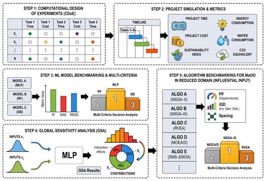
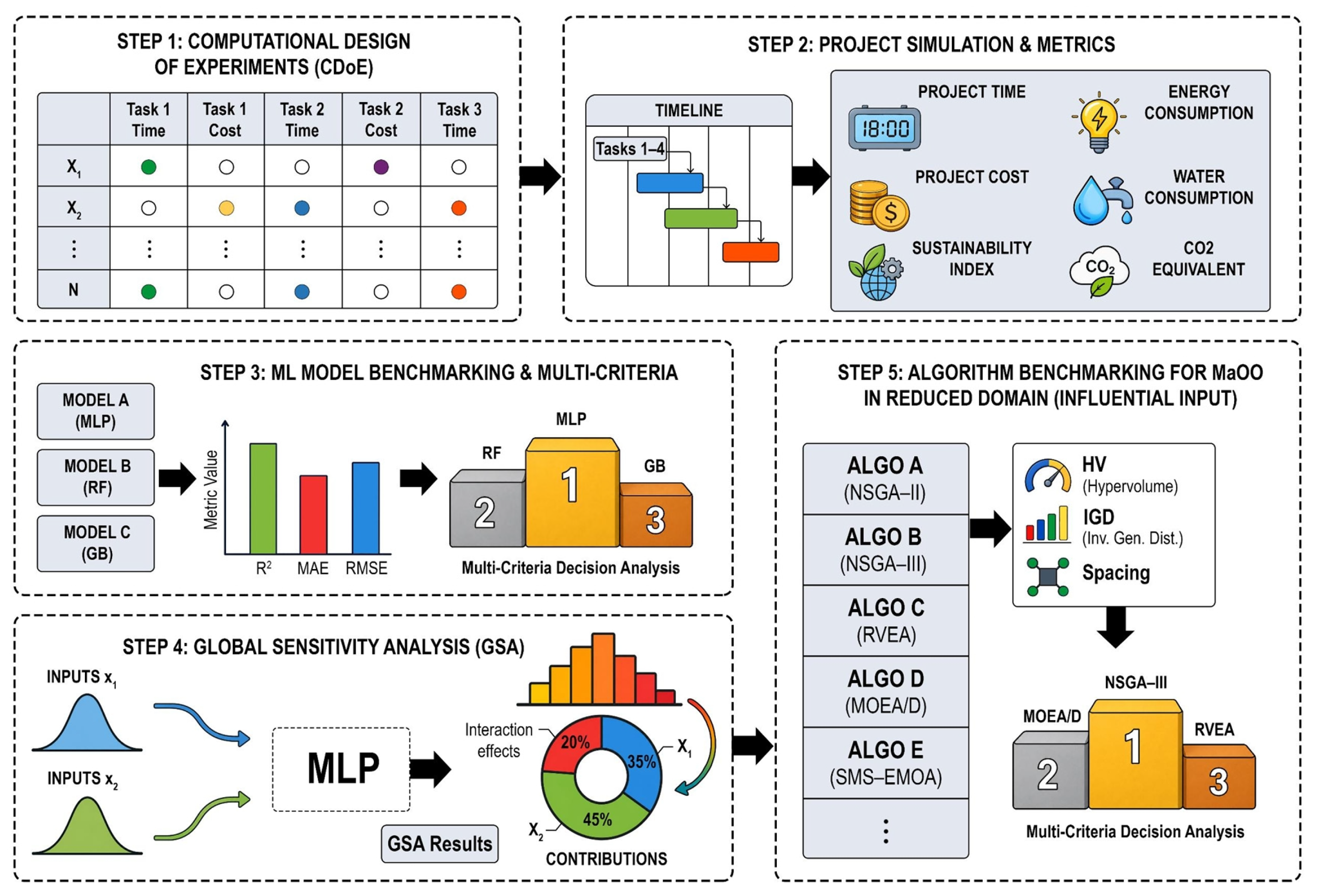
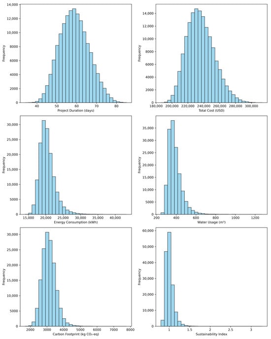
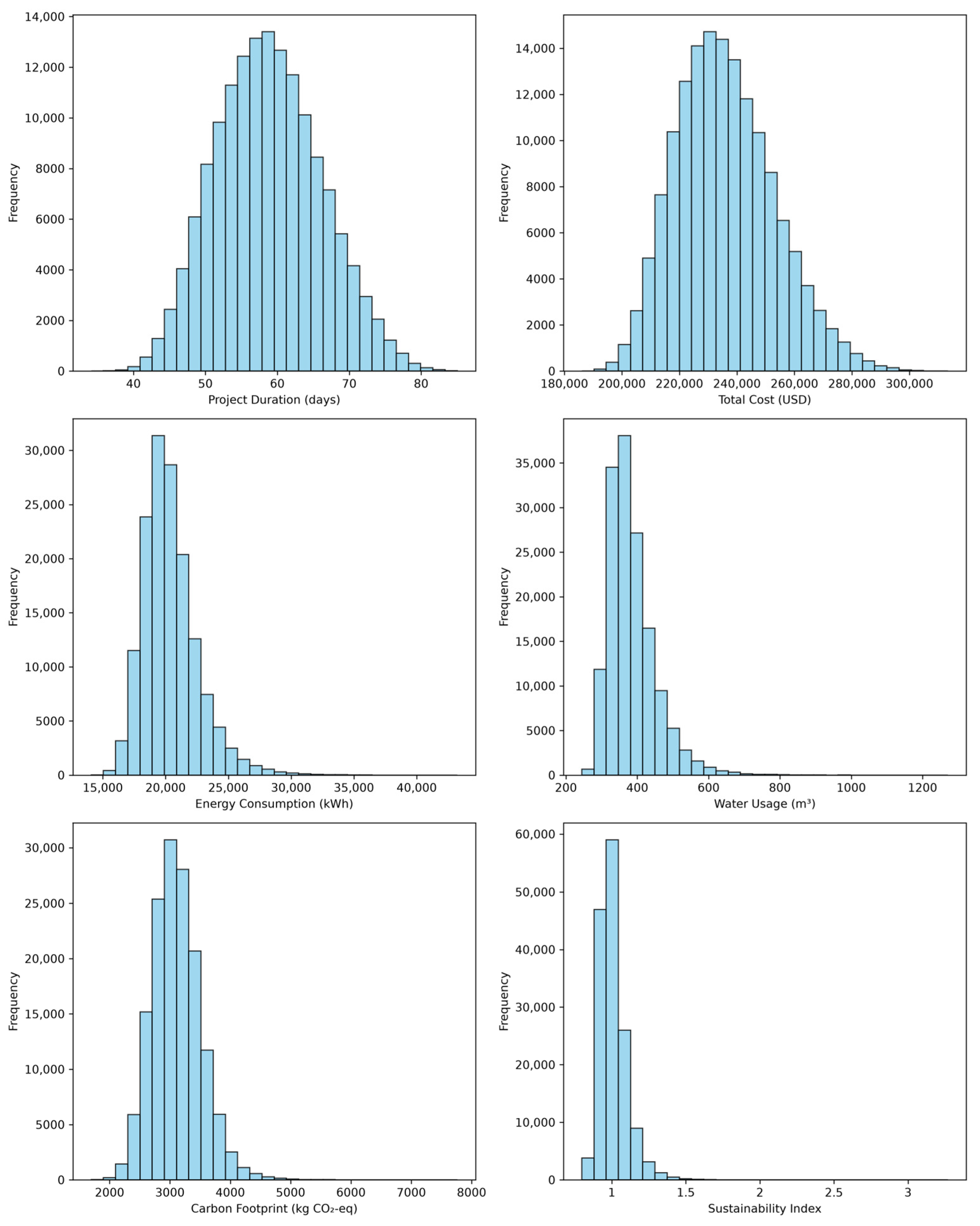
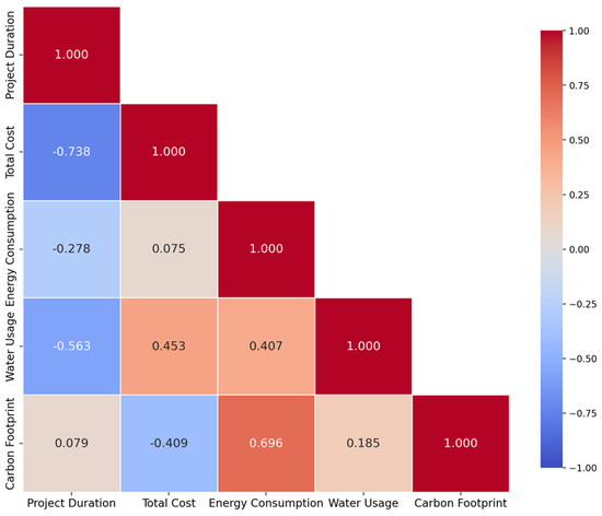
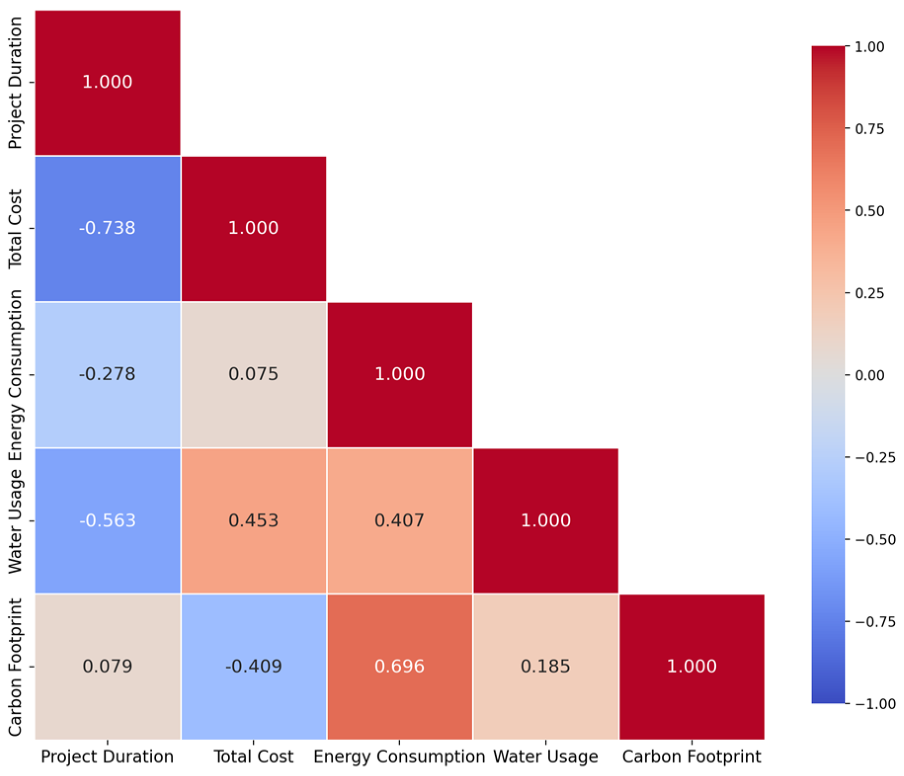
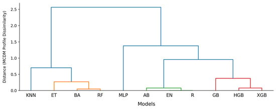
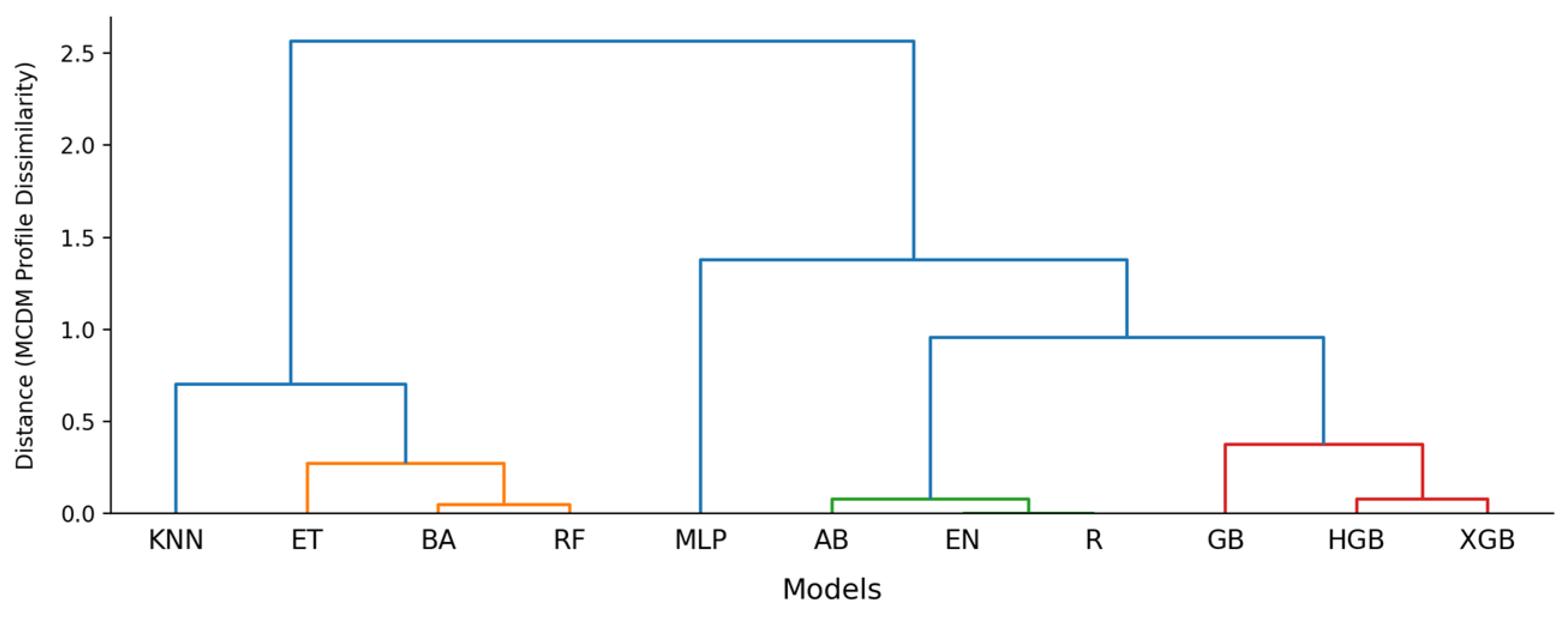
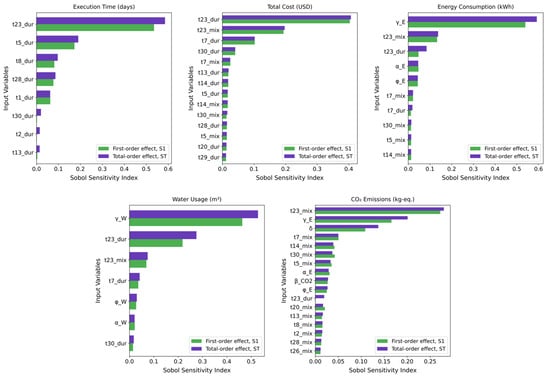
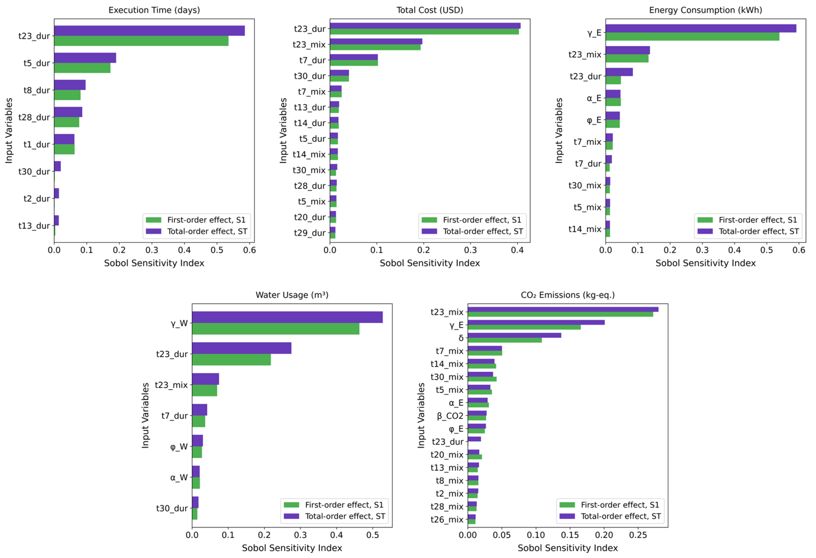

Disclaimer/Publisher’s Note: The statements, opinions and data contained in all publications are solely those of the individual author(s) and contributor(s) and not of MDPI and/or the editor(s). MDPI and/or the editor(s) disclaim responsibility for any injury to people or property resulting from any ideas, methods, instructions or products referred to in the content. |
© 2026 by the authors. Licensee MDPI, Basel, Switzerland. This article is an open access article distributed under the terms and conditions of the Creative Commons Attribution (CC BY) license.