


Abstract
Dynamic stability during human movement reflects interactions among body configuration, support conditions, mechanical state, and short-term state evolution. This study proposes a frame-wise stability score, S(t), integrating three dimensionless instability components: a height-adaptive extrapolated center of mass (XCoM)–base of support (BoS) geometric term, mechanical-energy deviation, and a Lyapunov-type state-trend term. The framework was evaluated using 24 HuMoD walking, running, kicking, and jumping trials from two participants, 26 HuMoD trials for sensitivity analysis, and 73 GAITEX trials. Task means followed the predefined biomechanical ranking (Spearman and Kendall = 1.000), which served as a consistency reference rather than an independent ground truth. Trial-level associations with margin of stability (MoS) and signed CoM–BoS distance were weak, whereas S(t) showed a negative association with center-of-pressure (COP) velocity (r = −0.667); COP velocity showed greater task discrimination (effect size 0.814 vs. 0.350). Ablation analysis showed the largest overall numerical effect for geometry, while trend contributed up to 28.77% of total instability locally. Tested parameter perturbations retained similar qualitative response patterns. These results support S(t) as an interpretable framework for organizing support geometry, mechanical-state deviation, and short-term state evolution on a common frame-wise scale; clinical and predictive validity require independent validation.
1. Introduction
Human dynamic stability is fundamental to gait analysis, rehabilitation assessment, movement-quality evaluation, and the construction of biomechanical features for fall-risk models. In this study, human dynamic stability refers to the capacity to maintain controlled whole-body motion while body configuration, support conditions, and the center-of-mass (CoM) state change over time. During walking, running, jumping, and rehabilitation exercises, the CoM moves relative to a time-varying base of support (BoS), defined by the body–ground contact region. The BoS changes as the contact condition transitions among double support, single support, and unsupported phases. Meanwhile, sensory information and neuromuscular actions are continuously integrated to regulate posture and movement, constituting the sensorimotor control process [1,2,3]. The biomechanical effects of sensorimotor control are reflected in CoM motion and support-state evolution, providing kinematic and support-state information for the quantitative characterization of human dynamic stability. Because CoM position and velocity, support configuration, mechanical state, and temporal evolution may change simultaneously, a single kinematic variable is generally insufficient to characterize human dynamic stability.
Existing approaches quantify different aspects of stability. Geometric measures, particularly the margin of stability (MoS) based on the extrapolated center of mass (XCoM) and the BoS, incorporate both CoM position and velocity, providing an interpretable description of the instantaneous relationship between body motion and the support boundary [4]. Center-of-pressure (COP) measures characterize postural regulation through the motion of the resultant ground-reaction force application point [5,6]. Measures of gait variability and local dynamic stability describe cycle-to-cycle fluctuations or the sensitivity of locomotor trajectories and are widely used in gait analysis [7,8,9,10,11]. Energy-related measures characterize mechanical-state variation and energy exchange during locomotion [12,13]. Stability assessment has also increasingly moved toward wearable and reduced-sensor configurations, including estimation from single body landmarks, pelvic motion, and inertial measurement units (IMUs) [14,15,16,17,18,19]. In parallel, data-driven approaches have been developed for gait-state and fall-risk classification [20,21].
These approaches provide useful but different stability information. Geometric measures directly characterize the relationship between the moving CoM state and the available support region, but they do not explicitly represent mechanical-energy deviation or the short-term direction of state evolution. COP-based measures are sensitive to postural regulation but depend on force-related measurements and are strongly influenced by support conditions. Sequence-level measures of gait variability and local dynamic stability are well suited to repeated locomotor cycles but are less direct for frame-wise assessment of non-stationary movements such as kicking, jumping, and movement transitions. Energy measures describe changes in mechanical state but do not by themselves indicate proximity to the support boundary. Data-driven models may provide classification capability, whereas their outputs do not necessarily correspond to an explicit biomechanical quantity. In practical measurement settings, kinematic reconstruction errors, gait-event detection errors, and task familiarization may further affect stability estimates [22,23,24,25]. These characteristics motivate a frame-wise assessment framework that represents different biomechanical aspects separately and subsequently integrates them within a common scoring form.
Based on this biomechanical rationale, the present study constructs a frame-wise description of human dynamic stability from three perspectives: geometric boundary, energy deviation, and state trend. Unlike approaches that use multiple stability features as sequence-level statistics or as inputs to classification or prediction models, the proposed framework defines three biomechanically interpretable descriptors at the frame level and transforms them into direction-consistent, dimensionless instability components. Geometric boundary describes the instantaneous spatial relationship between the velocity-adjusted CoM state and the BoS boundary, indicating proximity to the current mechanical support constraint. Energy deviation quantifies the departure of the current mechanical-energy state from the typical energy state of the same trial, capturing mechanical-state changes not directly represented by a geometric margin. State trend describes the short-term evolution of the CoM position–velocity state relative to a support-dependent reference region, characterizing the local direction of state change. Together, these descriptors represent spatial constraints, mechanical-state variation, and local temporal evolution within a unified frame-wise scoring scale.
Based on this framework, the main contributions of the study are threefold. First, a geometry–energy–trend framework is established in which the signed XCoM-BoS relationship, mechanical-energy deviation, and Lyapunov-like state trend are transformed into direction-consistent, dimensionless instability components and represented within a unified mathematical formulation. Second, a continuous and bounded frame-wise stability score, S(t), is constructed via weighted fusion of the three instability components followed by exponential mapping, providing a common numerical representation for temporal analysis within movement sequences and descriptive comparisons across movement conditions. Third, an analytical, label-free assessment method is developed by combining a height-adaptive XCoM formulation with energy- and trend-based descriptors. The method does not require instability labels or model training, providing a biomechanically interpretable framework for movement-state analysis and a methodological basis for future investigation of potential applications in rehabilitation monitoring and stability-related feature construction.
2. Materials and Methods
2.1. Biomechanical Rationale and Unified Stability Scoring Framework
Human dynamic stability during movement involves changes in the relationship between body motion and external support, variation in mechanical state, and local temporal evolution of the current motion state. To represent these aspects at the frame level, the present framework uses three descriptors: geometric boundary, energy deviation, and state trend. These descriptors characterize dynamic movement from the perspectives of spatial support constraint, mechanical-state variation, and local temporal evolution, respectively.
The geometric descriptor represents the instantaneous relationship between the velocity-adjusted CoM state and the currently available support region. Its biomechanical basis follows the extrapolated center of mass (XCoM) concept, in which both CoM position and horizontal velocity contribute to the relationship between the moving body state and the support boundary [4]. As XCoM approaches the boundary of the support region, the geometric margin decreases, whereas boundary crossing indicates that the extrapolated state lies outside the current support region. The descriptor therefore characterizes the spatial relationship between the moving body state and the current mechanical support constraint.
The energy descriptor quantifies departure of the current CoM-based mechanical state from the typical state of the same trial. Changes in CoM velocity and height cause this descriptor to vary over the course of movement, providing mechanical-state information in addition to the geometric boundary relationship. Its detailed definition, reference state, and normalization are presented in Section 2.3.
The trend descriptor characterizes local temporal change in the CoM position–velocity state [26] relative to a support-dependent reference state. Because the magnitude of an instantaneous state does not indicate its direction of change, the present framework combines a support-related position–velocity candidate quantity with its rate of change to describe whether the local state is increasing or decreasing. This descriptor therefore provides information on short-term state evolution in addition to the geometric and energy descriptions.
The three descriptors are converted into non-negative, dimensionless, and direction-consistent instability components and combined to obtain the total frame-wise instability:
where t denotes time or frame index; Ψ(t) is the total instability; Φg(t), Φe(t), and Φt(t) are the geometric, energy, and trend instability components, respectively; and λg, λe, and λt are their corresponding fusion weights.
Ψ(t) = λg ⋅ Φg(t) + λe ⋅ Φe(t) + λt ⋅ Φt(t)
A linear weighted form was adopted to keep the contribution of each dimensionless component directly interpretable on a common scale. For each component, the frame-wise contribution to total instability is explicitly given by λjΦj(t), allowing the numerical roles of the three terms to be compared and traced over time.
For the main analysis, λg = 0.5, λe = 0.3, and λt = 0.2 were used as a prespecified reference configuration, with λg + λe + λt = 1. This configuration establishes a modeling hierarchy by assigning the largest coefficient to the geometric term, followed by the energy and trend terms. With the component values and the other weights held fixed, a change Δλj in a given weight changes the final score by the multiplicative factor exp[−ΔλjΦj(t)].
Thus, the effect of a weight change depends directly on the magnitude of the corresponding component at that frame. Parameter-sensitivity analysis was used to examine the behavior of the score under perturbations around the reference configuration. The sum-to-one condition applies to the main-analysis configuration, whereas the remaining weights were held fixed in the ablation and one-factor sensitivity analyses.
Because the three instability components are non-negative, Ψ(t) ≥ 0. The total instability is then mapped to a continuous bounded stability score:
S(t) = exp(−Ψ(t)), S(t) ∈ (0,1]
When Ψ(t) = 0, S(t) = 1, and the score decreases monotonically as total instability increases.
Because −lnS(t) = Ψ(t), the additive contributions of the three components remain explicit on the negative-log scale. An equal increment ΔΨ in total instability produces the same multiplicative score factor exp(−ΔΨ). The exponential mapping therefore preserves the ordering defined by total instability while constraining the final score to a common bounded interval. The three components and their fusion process are illustrated in Figure 1.
Figure 1.
Biomechanical components and computational workflow of the proposed frame-wise stability score S(t). (a) Geometric component: the horizontal whole-body CoM position and velocity vC,h(t) are used to construct XCoM; dB(t) denotes the signed distance from XCoM to the current base-of-support (BoS) boundary, dref is the geometric reference distance, and the resulting geometric-instability component is Φg(t). (b) Mechanical-energy component: E(t) is the CoM-based mechanical-energy descriptor, Eref is the trial-specific reference value, DE(t) is the absolute deviation, Escale(t) is the energy-normalization scale, mE(t) is the dimensionless energy margin, and Φe(t) is the resulting energy-instability component. (c) Trend component: pC,h(t) and vC,h(t) denote the horizontal CoM position and velocity, respectively, and pr(t) is the support-dependent reference position; these quantities define the state candidate V(t), its rate of change , and the trend-instability component Φt(t), while t + Δt schematically denotes the subsequent local state. (d) The three dimensionless instability components are combined using the prespecified main-analysis weights 0.5, 0.3, and 0.2 to obtain total instability Ψ(t), which is subsequently mapped exponentially to the bounded frame-wise score S(t). Higher S(t) corresponds to lower combined instability, and vice versa. Curves and geometric positions are schematic.
The fixed parameters and implementation values used in the proposed method are summarized in Table 1. Their mathematical definitions, computational roles, and parameter sensitivity are described in the corresponding subsections. For ease of reference, the principal symbols and operators used throughout the framework are summarized in Appendix A (Table A1).
Table 1.
Principal protocol parameters of the proposed stability scoring framework.
2.2. Geometric Instability Based on the XCoM–BoS Boundary Relationship
Geometric instability characterizes the instantaneous spatial relationship between the velocity-adjusted CoM state and the current support region. All geometric calculations are performed in the common global Cartesian coordinate system used after preprocessing, with the y-axis defined as vertical and the x-z plane defined as horizontal. For a three-dimensional position vector p = [x, y, z]T, its horizontal projection is denoted by ph = [x, z]T. The whole-body CoM position pC(t) is obtained by mass weighting the segment CoM positions; its horizontal position and velocity are denoted by pC,h(t) and vC,h(t), respectively.
The geometric component is constructed in three steps. First, a height-adaptive XCoM is calculated from the horizontal CoM position and velocity together with the instantaneous CoM height. Second, the BoS is constructed according to the current foot–ground support state. Finally, the signed distance from XCoM to the BoS boundary is calculated and transformed into the dimensionless geometric-instability component Φg(t).
2.2.1. Height-Adaptive XCoM
The XCoM formulation is based on the linear inverted-pendulum approximation commonly used in dynamic-balance analysis [4]. In this approximation, the whole-body CoM is represented as a point mass above an equivalent support point, and horizontal motion is locally linearized near the upright configuration using the small-angle approximation. For either horizontal coordinate, the local relationship is expressed as follows:
Here, xC(t) and denote the horizontal CoM coordinate and its second time derivative, respectively; and xp(t) is the horizontal coordinate of the equivalent support point. The parameter ω0(t) is the characteristic rate of the linearized inverted-pendulum relation, with units of s−1, and is defined as follows:
where g = 9.81 m s−2 is gravitational acceleration and L(t) is the equivalent pendulum length at the current frame. Its reciprocal, 1/ω0(t), defines the characteristic time scale used for velocity extrapolation in XCoM. Accordingly, vC,h(t)/ω0(t) has units of length and represents the extrapolation displacement associated with the current horizontal CoM velocity.
Conventional XCoM calculations commonly use a fixed equivalent pendulum length. For movements involving substantial changes in CoM height, such as squatting and jumping, the present formulation updates the equivalent length frame by frame according to the vertical distance between the CoM and the ground:
where yC(t) is the vertical coordinate of the whole-body CoM and yg(t) is the ground height. Previous inverted-pendulum and dynamic-stability studies have related the characteristic pendulum length or CoM-related length scale to anthropometric dimensions such as body height or leg length [27,28,29]. Accordingly, L(t) is treated here as a positive length scale associated with the current body geometry. Because , very small or abnormally large values of L(t) would disproportionately affect the characteristic rate and the corresponding velocity-extrapolation scale of XCoM. The frame-wise CoM-to-ground distance is therefore constrained to 0.3–2.0 m. These values serve as broad protocol bounds that accommodate low body configurations and elevated CoM states while limiting the influence of extreme postures or kinematic-reconstruction artifacts on L(t) and the subsequent XCoM calculation.
L(t) = min{max[yC(t) − yg(t),Lmin],Lmax}
The horizontal XCoM position is then calculated as follows:
where pX(t) is the horizontal XCoM position, pC,h(t) is the horizontal whole-body CoM position, and vC,h(t) is the horizontal CoM velocity. The term vC,h(t)/ω0(t) converts the current velocity into an extrapolation displacement using the characteristic inverted-pendulum time scale, so that XCoM reflects both the instantaneous CoM position and its velocity-dependent extrapolation. Because L(t) is updated with CoM height, the velocity-extrapolation scale changes accordingly.
In Figure 1a, the displacement from CoM to XCoM corresponds to vC,h(t)/ω0(t); the subsequent geometric calculation uses the relationship between pX(t) and the current BoS boundary.
2.2.2. BoS Construction and Foot–Ground Contact Detection
The BoS is constructed from an approximate horizontal support region of the feet that are in contact with the ground at the current frame. Four fixed plantar template points are assigned to each foot to approximate its support outline, corresponding to the heel, medial forefoot, lateral forefoot, and toe. The ankle position is used as the translational reference for the template, and its horizontal dimensions are based on adult foot morphology [30]. The present template corresponds to a foot length of approximately 25 cm and the same template dimensions are used for all trials. The corresponding horizontal offsets of the plantar support-template points are summarized in Table 2.
Table 2.
Horizontal offsets of the plantar support-template points used for BoS construction.
The values shown define the nominal template for one foot; the mediolateral direction is mirrored for the opposite side.
For foot side s ∈ {L, R} and template point j ∈ {1,…,4}, the horizontal position of the support-template point is defined as follows:
where is the horizontal position of the left or right ankle, is the fixed horizontal offset of template point j relative to the ankle, and is the resulting horizontal template point used for BoS construction. The horizontal projection operator Πh[⋅], defined above, maps three-dimensional positions onto the horizontal plane. The two feet use the same longitudinal dimensions, with the mediolateral direction mirrored between sides. The template therefore translates with the ankle position to provide a planar approximation of the foot-support region at each frame.
Foot–ground support is determined at the foot level. Let s(t) ∈ {0, 1} denote whether foot s contributes its support template to the BoS at time t, with s(t) = 1 for a supported foot and s(t) = 0 otherwise. Reliable left/right contact events are used directly when provided by the dataset. When such events are unavailable but vertical ground-reaction force data are available, the support state is determined as follows:
where Fv,s(t) is the vertical ground-reaction force associated with foot s and Fth = 20 N is the force threshold.
When neither contact events nor corresponding ground-reaction force data are available, a kinematic criterion based on ankle height relative to the ground is used:
where ha,s(t) is the ankle height relative to the ground and hth = 0.03 m is the height threshold used in the present computational protocol.
Here, s(t) denotes the foot-level support state of foot s, which determines whether the corresponding template points are included in the current BoS construction. When s(t) = 1, all four template points of that foot are included in the current support-point set; when s(t) = 0, they are excluded. The present criterion represents support at the foot level, while the four-point plantar template provides the corresponding geometric approximation of the support region.
The set of active horizontal support-template points is given by:
The current BoS is defined as the convex hull of this finite point set:
where Conv(⋅) denotes the smallest convex set containing the specified planar points and B(t) is the BoS polygon at the current frame. The convex hull is computed using the Quickhull algorithm [31].
B(t) = Conv{(t)}
When neither foot is in the support state, (t) is empty and no foot–ground BoS is defined for that frame. The geometric-instability treatment of double-flight phases is described separately in Section 2.2.3.
The plantar template points, foot-level support state, and resulting BoS geometry are illustrated schematically in Figure 1a.
2.2.3. Signed XCoM–BoS Distance and Geometric Instability
During supported phases with a valid BoS, the position of XCoM relative to the BoS boundary characterizes the geometric relationship between the velocity-adjusted motion state and the available support region. An unsigned Euclidean distance cannot distinguish whether XCoM remains inside the BoS or has crossed its boundary. A sign convention is therefore applied to the minimum boundary distance:
where dB(t) is the signed XCoM-to-BoS boundary distance, ∂B(t) denotes the boundary of the BoS polygon, intB(t) denotes its interior, q is a point on the boundary, and ‖·‖2 denotes the Euclidean norm.
Under this convention, dB(t) > 0 when XCoM lies inside the BoS and represents the internal geometric margin to the nearest boundary. At the boundary, dB(t) = 0. After XCoM crosses the boundary, dB(t) < 0, and its magnitude represents the boundary-exceedance distance. The signed quantity therefore combines boundary distance and inside/outside location within a single geometric variable.
For frames with a valid BoS, dB(t) is transformed into the dimensionless geometric-instability component:
where dref = 0.12 m is the geometric reference distance that sets the spatial normalization scale for boundary approach within the BoS and Φg,max = 2.0 is the upper bound of the geometric-instability component.
When dB(t) ≥ dref, geometric instability is zero. As XCoM approaches the BoS boundary from the reference distance, Φg(t) increases continuously from 0 to 1, with dB(t) = 0 corresponding to Φg(t) = 1. After boundary crossing, dB(t) < 0, so , and geometric instability increases with boundary-exceedance distance until reaching Φg,max. The piecewise mapping therefore represents internal margin, boundary approach, and boundary exceedance on a common dimensionless scale.
During double-flight phases in running and jumping, neither foot provides ground support and no BoS boundary is available for evaluating dB(t). The geometric component is therefore assigned the predefined unsupported-phase value Φg(t) = γflt = 0.5, where γflt is the geometric-instability protocol value for double flight. This rule provides a defined geometric component during unsupported frames while keeping the flight treatment separate from the boundary-distance calculation used during supported phases.
Figure 1a illustrates the correspondence between dB(t) and Φg(t) for XCoM locations inside, at, and outside the BoS boundary.
2.3. Energy Instability Based on Mechanical-Energy Deviation
Energy instability characterizes the departure of the current CoM-based mechanical state from the typical state of the same trial. During movement, changes in whole-body CoM velocity and height accompany phases such as acceleration, push-off, flight, and landing, providing mechanical-state variation that differs from the geometric relationship to the support boundary [13]. A frame-wise mechanical-energy descriptor is therefore constructed, and its deviation from the trial-specific reference state is subsequently transformed into the dimensionless energy-instability component.
2.3.1. CoM-Based Mechanical-Energy Descriptor
To characterize the mechanical state of the movement frame by frame, a mechanical-energy descriptor E(t) is defined from the kinetic and gravitational-potential terms used in the present model:
where E(t) is the mechanical-energy descriptor, K(t) is the kinetic-energy term used in the descriptor, and U(t) is the gravitational-potential term.
E(t) = K(t) + U(t)
The kinetic-energy term represents bulk whole-body translation at the CoM level and is calculated from the three-dimensional whole-body CoM velocity:
where is the sum of the modeled segment masses, vC(t) is the three-dimensional whole-body CoM velocity, and Ns = 15 is the number of modeled body segments. This term characterizes bulk translational motion at the whole-body CoM level and is used in the subsequent calculation of within-trial mechanical-state deviation.
Taking the ground height in the global coordinate system as the zero-potential reference, the gravitational-potential term is expressed as follows:
where yC(t) is the vertical coordinate of the whole-body CoM and yg(t) is the ground reference height used in the calculation.
U(t) = Mg[yC(t) − yg(t)]
The whole-body CoM position and velocity are obtained by mass weighting the modeled body segments:
where mi, pi(t), and vi(t) are the mass, CoM position, and CoM velocity of segment i, respectively. Mass and CoM-location parameters for the 15 modeled segments were specified according to the Winter anthropometric model [32] together with participant height and body mass.
2.3.2. Time-Varying Energy Normalization Scale
Mechanical-energy deviation has units of energy, and its magnitude depends on both the modeled mass M and the current body geometry. To express this deviation on a common dimensionless scale, a frame-wise energy normalization scale is constructed using the equivalent pendulum length L(t) and the geometric reference distance dref defined above.
The reference distance dref and the current equivalent length L(t) define a reference inclination angle arctan[dref/L(t)]. Based on this reference geometry, the corresponding gravitational potential-energy change is used to construct the energy normalization scale at the current frame, Escale(t), with units of J:
where M is the sum of the modeled segment masses, g is gravitational acceleration, L(t) is the equivalent pendulum length defined in Equation (5), and dref is the geometric reference distance used in Equation (11).
When dref is small relative to L(t), . Together with the small-angle approximation 1 − cosθ≈θ2/2, Equation (16) becomes:
Thus, Escale(t) varies with the modeled mass M and the current equivalent pendulum length, while the use of dref links the normalization scale to the same reference distance used in the geometric component.
2.3.3. Mechanical-Energy Deviation and Energy Instability
To define the typical mechanical state of each trial, the median of E(t) over all valid frames is used as the reference value:
where Eref is the reference value of the mechanical-energy descriptor for the current trial. The median reduces the influence of short-duration high-amplitude changes associated with events such as landing and rapid push-off, thereby representing the typical energy level of the movement sequence.
Eref = mediant{E(t)}
Departure of the current state from this reference is defined as follows:
where DE(t) is the absolute deviation of the mechanical-energy descriptor. The energy component characterizes the magnitude of departure from the trial-specific reference state; deviations above and below Eref therefore enter the subsequent calculation according to their absolute magnitude.
DE(t) = |E(t) − Eref|
A dimensionless energy margin is then constructed using the time-varying energy scale:
In the numerical implementation, mE(t) is bounded to the interval [−2, 1]. When E(t) is close to Eref, DE(t) is small and mE(t) approaches 1. When DE(t) = Escale(t), mE(t) = 0; when the deviation exceeds the current normalization scale, mE(t) < 0.
The dimensionless energy-instability component is then defined as follows:
When the mechanical-energy descriptor is close to its trial-specific reference value, Φe(t) approaches zero. As the deviation increases, mE(t) decreases and the quadratic branch provides a continuous increase in energy instability over 0 ≤ mE(t) < 1. When mE(t) < 0, the deviation exceeds the current normalization scale, and the logarithmic branch represents further increases while reducing the numerical influence of extreme instantaneous deviations. Equation (21) is continuous at both mE(t) = 0 and mE(t) = 1.
In the computational implementation, the frame-wise Φe(t) sequence obtained from Equation (21) is smoothed using a three-frame moving average before entering the fusion in Equation (1).
2.4. Trend Instability Based on State Evolution
The geometric component describes the spatial relationship between the current motion state and the support boundary, whereas the energy component describes the magnitude of mechanical-state deviation from the typical state of the trial. Continuous movement also involves a local direction of state evolution. The trend component therefore combines a state candidate with its rate of change to characterize both the CoM-state deviation relative to the current support reference and its local temporal evolution.
2.4.1. Support-Dependent Reference State and Candidate Function
The horizontal CoM reference position, pr(t), is determined frame by frame from the current support state. During single support, pr(t) is the horizontal position of the supporting ankle; during double support, it is the midpoint of the left and right ankle positions; and during double flight, it is the current horizontal whole-body CoM position. The reference position therefore evolves with the support condition throughout the movement.
Based on this reference state, a Lyapunov-type state candidate is constructed from the horizontal CoM position deviation and velocity:
where V(t) is the state candidate; pC,h(t) and vC,h(t) are the horizontal whole-body CoM position and velocity, respectively; pr(t) is the support-dependent reference position; and wp and wv control the relative scaling of the position-deviation and velocity terms, respectively. The present formulation uses wp = 1.0 and wv = 0.3. With position expressed in m and velocity in m/s, wv provides the corresponding squared-time scaling so that the two quadratic terms are dimensionally compatible.
V(t) varies with both the spatial deviation of the CoM from the current support reference and its horizontal motion. A larger V(t) indicates a larger position–velocity state deviation, whose subsequent temporal change is used to characterize local state evolution.
2.4.2. State Rate of Change and Nondimensionalization
The temporal rate of change of the candidate quantity is defined as follows:
where represents the local temporal rate of change of the state candidate. Positive values indicate that V(t) is increasing, whereas negative values indicate that it is decreasing. For discrete motion data, is obtained using the Savitzky–Golay derivative procedure described in Section 2.5.
To reduce the influence of differences in candidate magnitude among trials, the mean absolute candidate value over all frames of the preprocessed trial sequence is used as the state-normalization reference scale:
where Vref is the trial-specific state reference scale, Nfrm is the number of frames in the preprocessed trial sequence, tk is the time corresponding to frame k, and εV = 10−8 m2 is a small positive numerical regularizer.
The candidate quantity and its rate of change are then normalized as follows:
where is the normalized state candidate, is the normalized rate of change, and is the fixed derivative-normalization scale, set to , and is a small positive numerical regularizer.
2.4.3. Trend Instability
Trend instability is determined jointly by the normalized state deviation and its positive rate of change:
where Φt(t) is the dimensionless trend-instability component and Φt,max = 1.5 is its upper bound.
For the instantaneous value defined by Equation (26), gives a zero trend term. When , the trend term increases jointly with the normalized state deviation and its positive rate of change and is bounded by Φt,max.
To reduce short-duration fluctuations associated with frame-wise derivative estimation, the trend-instability sequence obtained from Equation (26) is subsequently smoothed using a five-frame moving average. The smoothed Φt(t) sequence is used in the fusion defined by Equation (1).
2.5. Datasets, Computational Implementation, and Validation Design
The proposed score was evaluated using two public human-motion datasets: HuMoD and GAITEX. HuMoD provides whole-body kinematics and ground-reaction force data for walking, running, kicking, jumping, squatting, and other dynamic tasks. These data enable an analysis of the response of S(t) to support state, movement speed, and CoM-height changes, while facilitating comparisons with classical stability metrics under matched conditions. GAITEX includes rehabilitation exercises, normal gait, and orthosis-assisted gait and was used to examine computational applicability across different movement forms and support conditions.
HuMoD dataset. HuMoD [33] contains records from two healthy participants: Subject A (female, 57.3 kg, 1.61 m) and Subject B (male, 84.8 kg, 1.79 m). A total of 26 usable trials were analyzed. Among them, 24 walking, running, kicking, and jumping trials were used for frame-wise response analysis, task ranking, classical-metric comparison, and ablation analysis (12 walking, 8 running, 2 kicking, and 2 jumping trials). Two additional squat trials were included in the sensitivity analysis, giving 26 trials in total. HuMoD statistical summaries used individual trials as the analysis unit. The 24 primary trials comprise repeated observations from two participants; accordingly, the trial-level statistical results describe the analyzed trial set and are interpreted in light of the resulting within-participant dependence.
GAITEX dataset. GAITEX [34] contains records from rehabilitation exercises, normal gait, and orthosis-assisted gait from healthy participants and provides motion information derived from optical motion capture and inertial measurements, together with OpenSim inverse-kinematics results. All 73 available trials were used: 19 resisted-dorsiflexion (rd), 18 resisted-gait-simulation (rgs), 18 normal-gait (ng), and 18 gait-with-orthosis (gwo) trials. Based on task type, rd and rgs were combined as the rehabilitation group (37 trials), ng formed the normal-gait group (18 trials), and gwo formed the orthosis-assisted-gait group (18 trials). No additional truncation or group-size matching was applied.
Data processing and computational implementation. The computational analyses and figure generation were performed in Python 3.9.8 using NumPy 1.24.3, SciPy 1.12.0, pandas 2.3.3, and Matplotlib 3.8.2. Both datasets were converted to a common kinematic input format and resampled to 50 Hz. Position trajectories were smoothed using a Savitzky–Golay filter with a 15-frame window and third-order polynomial. CoM velocity, segment velocity, and state derivatives were obtained by differentiating the smoothed trajectories. Resampling was restricted to the valid time range of each trial to preserve the original sequence boundaries.
For HuMoD, left/right foot-contact events provided by the dataset were used preferentially; when contact events were unavailable but bilateral vertical ground-reaction forces were available, a 20 N threshold was applied independently to each foot. GAITEX does not provide plantar ground-reaction force data directly corresponding to the present computation. Therefore, contact during normal and orthosis-assisted gait was determined from ankle height relative to the ground using a 0.03 m threshold, and the resulting binary contact sequence was smoothed over five frames to reduce isolated state transitions. Rehabilitation tasks were performed primarily under standing-support conditions, and their support states were specified according to the corresponding task conditions. Because GAITEX lacks synchronized plantar vertical ground-reaction force data for this criterion, the performance of ankle-height contact detection in orthosis-assisted gait was not evaluated separately. This rule was used as a kinematic approximation of foot–ground contact for GAITEX.
For data without ground-reaction force information, the kinematic contact criterion described in Section 2.2 was used in place of force-based contact detection. Trials lacking the variables required to compute the stability score were excluded from subsequent statistical analysis. No additional subsampling was performed to balance task counts; all available trials that met the required input conditions and allowed computation of the stability score were included in the corresponding analyses.
After preprocessing, whole-body CoM, CoM velocity, adaptive XCoM, BoS, signed XCoM–BoS distance, the mechanical-energy descriptor, and the trend candidate were calculated along each trial, followed by Φg(t), Φe(t), Φt(t), total instability Ψ(t), and S(t). The final score is evaluated frame by frame; the trial-specific reference quantities Eref and Vref are obtained from the valid frames within each trial, while smoothing and derivative estimation use the temporal windows described above.
Validation design and statistical analysis. The proposed stability score was evaluated from five perspectives. First, frame-wise S(t) responses and task-level score characteristics were examined in 24 HuMoD walking, running, kicking, and jumping trials. An expected stability order was defined from task-specific support states, CoM movement speed, and flight-phase characteristics to assess whether task-level scores followed relative trends consistent with these biomechanical features. Because these factors are also related to variables used in S(t), the predefined order was used as a reference for biomechanical consistency, whereas independent validity requires external criteria. Second, S(t) was compared with six established stability-related metrics using the same HuMoD trials, task grouping, and preprocessing: MoS/XCoM–BoS stability margin, signed CoM–BoS distance, mechanical-energy coefficient of variation, gait-cycle variability, COP velocity, and GRF symmetry. Signed CoM–BoS distance was defined as the minimum signed Euclidean distance from the horizontal projection of the whole-body CoM to the current BoS boundary, with positive values inside the BoS and negative values outside. It used the same BoS construction as the XCoM–BoS metric but did not include the velocity-extrapolation term. Pearson correlation coefficients were used to summarize linear associations between trial-level mean S(t) and the classical metrics, with nominal 95% confidence intervals calculated using Fisher’s z transformation; Spearman rank correlations were used to summarize monotonic associations. Because the HuMoD trial set comprises repeated measurements from only two participants, the associated p-values and confidence intervals are reported as exploratory summaries of the analyzed trial set rather than as population-level inferential evidence.
Task-ranking consistency and task discrimination were evaluated separately. Ranking consistency was quantified using Spearman and Kendall coefficients between task-mean metric rankings and the expected stability order. Before this analysis, metric directions were standardized so that larger direction-adjusted values represented higher relative stability; COP velocity, mechanical-energy coefficient of variation, gait-cycle variability, and GRF symmetry were reversed where required according to their physical interpretation.
Between-task separation was summarized using the Kruskal–Wallis H statistic, its nominal p-value, and an effect size based on the H statistic. The effect size was defined as follows:
where is the effect size for the Kruskal–Wallis test, HK is the Kruskal–Wallis statistic, k is the number of task categories, and Nobs is the total number of trials included in the analysis. Negative effect-size estimates were set to zero for reporting. Given the repeated observations within participants in HuMoD, these task-level statistics are used primarily to characterize task separation within the analyzed dataset.
Third, ablation analysis was performed on the same 24 HuMoD trials used for task comparison. The full model used the main-analysis weights λg = 0.5, λe = 0.3, and λt = 0.2. The geometric, energy, or trend component was removed in turn, and geometry-only and energy-only models were also evaluated. Remaining weights were not renormalized after component removal, allowing the influence of each component to be observed under the common main-model weighting scheme. Fourth, parameter sensitivity was assessed using all 26 HuMoD trials. λg, λe, λt, and the geometric reference distance dref were perturbed individually by ±20%, with all other parameters fixed at baseline. Effects were evaluated from the correlation between S(t) and MoS, descriptive task separation, and changes in the score distribution. For sensitivity analysis, the one-way analysis of variance (ANOVA) F statistic computed from trial-level mean S(t) across activity groups was used as a descriptive measure of task separation. Fifth, all 73 GAITEX trials were used to compare S(t) distributions across rehabilitation, normal gait, and orthosis-assisted gait, thereby examining score behavior under different movement and support conditions. Trial-mean S(t) was used as the task-level descriptor together with the trial-level distributions.
3. Results
3.1. Frame-Wise Responses and Score Distributions Across Movement Tasks
Using the 24 HuMoD trials, frame-wise S(t) responses were first examined during walking, running, kicking, and jumping. Figure 2 shows S(t), foot-contact state, signed XCoM–BoS distance, and energy margin over time for representative trials. For unsupported frames without a valid BoS, signed XCoM–BoS distance is not displayed as a physical distance to avoid interpreting the unsupported state as an actual boundary distance.
Figure 2.
Representative frame-wise stability scores and associated biomechanical variables across four HuMoD movement tasks. Panels (a–d) show representative walking, running, kicking, and jumping trials, respectively. From top to bottom, each panel displays the frame-wise stability score S(t), left- and right-foot contact states, the signed XCoM–BoS boundary distance dB(t), and the dimensionless energy margin mE(t). The binary contact traces indicate supported and unsupported states for the left and right feet. The blue, green solid, magenta dashed, brown, and orange traces represent S(t), left-foot contact, right-foot contact, signed XCoM–BoS boundary distance, and energy margin, respectively. Positive dB(t) indicates that XCoM lies inside the current BoS, dB(t) = 0 denotes the BoS boundary, and negative dB(t) indicates boundary exceedance. Gray shading denotes intervals in which neither foot is classified as supported; in running and jumping, these intervals include double-flight phases. Representative support/contact transitions and unsupported or double-flight intervals are annotated to illustrate the temporal correspondence among support state, biomechanical variables, and S(t). During frames without a valid BoS, dB(t) is not displayed as a physical boundary distance.
During walking, S(t) showed repeated cyclic changes with single support, double support, and their transitions. During running, the score exhibited larger frame-wise fluctuations during sustained rapid motion and cyclic support transitions. Kicking generally maintained higher scores, with local decreases around foot-contact transitions and rapid-swing phases. During jumping, repeated double-flight and re-establishment of support produced pronounced cyclic support transitions; S(t) fluctuated accordingly during continuous jumping, with local changes near take-off and landing. These frame-wise results show that S(t) varies continuously with task-dependent changes in support configuration and movement state while remaining within a common bounded range.
The trial-level mean S(t) distributions for the four tasks are shown in Figure 3a, with the summary statistics presented in Table 3. The mean S(t) values were 0.7014, 0.5559, 0.4754, and 0.4576 for kicking, jumping, walking, and running, respectively, matching the predefined task-stability order. Within the current HuMoD task set, the task-level mean S(t) therefore followed the predefined stability order, reflecting the relative response of the score to differences in support state, movement speed, and dynamic phase.
Figure 3.
Trial-level task distributions and normalized cycle profiles of S(t) in HuMoD. (a) Trial-level mean S(t) distributions for walking (n = 12), running (n = 8), kicking (n = 2), and jumping (n = 2). Individual points represent trial-level mean scores, boxplots summarize the corresponding task distributions, and dark diamond markers indicate task means, with the mean values annotated. (b) Mean normalized-cycle profiles for walking (941 cycles), running (602 cycles), and kicking (78 cycles), with each cycle defined between consecutive right-foot contact events. Shaded bands denote ±1 SD across the valid cycles at each normalized-cycle position. Jumping yielded three valid cycles under this definition and was not included in the normalized-cycle profiles.
Table 3.
Trial counts, mean S(t), and predefined stability levels across HuMoD movement tasks.
Figure 3b further shows the normalized-cycle S(t) profiles for walking, running, and kicking, defined between consecutive right-foot contact events. These profiles are based on 941, 602, and 78 valid cycles, respectively. Jumping yielded only three cycles satisfying this definition and was not included in the normalized-cycle profiles.
Because kicking and jumping comprised only two trials each, the task means in Table 3 are intended to describe agreement between S(t) and the predefined task order within the current HuMoD dataset, rather than establish general population-level stability grades. Although the participant-level sample was limited, the multi-task and frame-wise results provide direct data for evaluating score responses across different support and movement states.
3.2. Associations with Classical Stability Metrics, Ranking Consistency, and Task Discrimination
To examine the relationship between S(t) and established stability-related metrics, MoS/XCoM–BoS stability margin, signed CoM–BoS distance, mechanical-energy coefficient of variation, gait-cycle variability, COP velocity, and GRF symmetry were calculated for the same 24 HuMoD trials and correlated with trial-level mean S(t), as shown in Table 4.
Table 4.
Trial-level associations between S(t) and classical stability-related metrics in HuMoD (N = 24).
S(t) had a Pearson correlation of 0.118 with MoS (nominal p = 0.582) and 0.119 with signed CoM–BoS distance (nominal p = 0.580), with the corresponding Spearman correlations also near zero. Thus, within the analyzed trial set, the fused score did not show a simple one-to-one linear or monotonic relationship with either geometric margin. The geometric boundary is one component of S(t), while the energy and state-trend terms also contribute to the resulting frame-wise score.
S(t) showed a negative association with COP velocity, with Pearson r = −0.667 (nominal p = 3.76 × 10⁻⁴) and Spearman ρ = −0.720 (nominal p = 7.2 × 10⁻⁵). This negative relationship is consistent with the opposite numerical directions of the two measures: larger COP velocity indicates greater center-of-pressure motion, whereas lower S(t) corresponds to greater fused instability in the present framework. The result therefore indicates a negative association between the two measures within the analyzed trial set.
Gait-cycle variability had a Pearson correlation of 0.622 with S(t) (nominal p = 0.00117), whereas the Spearman correlation was near zero (ρ = −0.008, nominal p = 0.971). The difference between the two association measures indicates the absence of a stable overall monotonic relationship within the analyzed trial set, suggesting sensitivity to task-specific data ranges and aggregation scales. Gait-cycle variability summarizes fluctuations across repeated cycles, whereas S(t) retains frame-wise state changes within the movement sequence. Trial-level associations of mechanical-energy CV and GRF symmetry with S(t) were weak and did not indicate a strong one-to-one relationship.
Using task-mean metric values, ranking consistency with the predefined stability order and task discrimination across the four tasks were then evaluated separately, as shown in Table 5. For task-mean ranking, S(t) achieved Spearman and Kendall consistencies of 1.000, exactly matching the predefined order. The corresponding values were 0.949 and 0.913 for COP velocity, and 0.400 and 0.333 for both MoS/XCoM–BoS stability margin and signed CoM-BoS distance. Thus, S(t) showed the highest ranking consistency with the predefined order in the current four HuMoD tasks.
Table 5.
Task-ranking consistency and task discrimination of S(t) and classical stability-related metrics.
Task-ranking consistency and task discrimination describe different aspects of metric behavior. For S(t), the four-task comparison yielded a Kruskal–Wallis H statistic of 9.999, a nominal p-value of 0.0186, and an effect size of 0.350. Its task-discrimination effect size was similar to those of the MoS/XCoM–BoS stability margin and signed CoM–BoS distance (H = 9.917, effect size = 0.346). COP velocity showed greater task discrimination (H = 19.284, effect size = 0.814), while mechanical-energy CV had an effect size of 0.479. Accordingly, the metrics showed different quantitative emphases across the four HuMoD tasks: COP velocity had the larger task-discrimination effect size, whereas S(t) showed the highest consistency with the predefined task order while providing a bounded frame-wise representation.
3.3. Ablation Results for the Geometric, Energy, and Trend Components
Ablation analysis of the geometric, energy, and trend components was performed on the same 24 HuMoD trials used for task comparison. The full model used the main-analysis weights. Each component was removed in turn, and geometry-only and energy-only models were also evaluated. Original component weights were retained without renormalizing the remaining weights, allowing direct assessment of each component under the common full-model weighting scheme, as shown in Table 6.
Table 6.
Ablation effects of geometric, energy, and trend components on trial-level mean S(t) in HuMoD.
The full model had a trial-level mean S(t) of 0.4950. Removing geometry increased the mean S(t) to 0.7702 (+0.2751), representing the largest change among the three single-component ablations. Removing energy increased the mean to 0.6260 (+0.1310), whereas removing trend increased it to 0.5041 (+0.0091). Because all three instability components contribute to total instability as non-negative additive terms, score increases after removal are consistent with the model definition. The different magnitudes show that, under the current weights and HuMoD trials, removal of the geometric component produced the largest numerical change in the mean score, followed by removal of the energy component, whereas removal of the trend component had a much smaller effect on the trial-level mean.
With geometry alone, the mean S(t) was 0.6378; with energy alone, it was 0.7895. Both single-component models produced higher mean scores than the full model, reflecting the accumulation of the non-negative instability components under the current fixed weighting scheme. Geometry and energy showed different numerical contribution magnitudes, while the full model additionally incorporated the short-term state-evolution term.
The trend component had a small effect on trial-level mean scores but was not uniformly negligible over time. Across the 24 HuMoD trials, the mean proportion of frames with nonzero trend instability was approximately 70.1%. In Subject A’s 4.0 m/s running trial, trend instability reached 1.5 at t = 98.740 s, giving a weighted trend contribution of 0.300. Total instability at that frame was 1.043, so trend accounted for 28.77% of the total. This example shows that the numerical effect of the trend component is concentrated during local rapid state evolution: although its influence on trial-level mean scores is small, it can make an appreciable local contribution to total instability at specific instants.
Overall, under the current weighting configuration and HuMoD trials, the ablation results showed different numerical contribution magnitudes among the three components: geometry produced the largest overall change, energy produced a smaller but appreciable overall change, and trend had a limited effect on trial-level means while contributing more noticeably during selected local dynamic transitions.
3.4. Parameter Sensitivity
Using all 26 HuMoD trials, the geometric, energy, and trend weights and the geometric reference distance were perturbed individually by ±20%. The associations between S(t) and MoS, descriptive task separation, and score-distribution changes under each parameter condition are summarized in Table 7.
Table 7.
Sensitivity of S(t) to ±20% perturbations of principal protocol parameters in HuMoD.
Across all tested parameter ranges, the association between S(t) and MoS remained positive, with correlation coefficients of 0.246–0.311 overall. The ranges were 0.281–0.291 for geometric-weight perturbation, 0.275–0.290 for energy-weight perturbation, 0.284–0.285 for trend-weight perturbation, and 0.246–0.311 for geometric-reference-distance perturbation. Within the tested ±20% perturbation ranges, none of the parameter changes reversed the direction of the association with MoS. The directional relationship therefore remained consistent over the examined parameter ranges, while the fused score retained numerical characteristics distinct from MoS alone.
The effects on task-separation statistics were also limited. The statistic remained 22.9 under trend-weight perturbation (0.0% variation), geometric-reference-distance perturbation yielded 21.7–23.1 (6.1% variation), and geometric- and energy-weight perturbations yielded variations of 16.0% and 20.0%, respectively. Thus, task-separation statistics remained within similar ranges across the tested conditions. Trend weight produced the smallest change, the geometric reference distance had a limited effect, and the larger numerical effects of geometric and energy weights were consistent with their greater global contributions in the ablation analysis.
Across all parameter perturbations, most trial-mean S(t) values remained within [0.4, 0.8]. The proportion was 96–100% for trend- and energy-weight perturbations, 88–100% for geometric-weight perturbation, and 85%–100% for the geometric reference distance. Therefore, within the tested ±20% ranges, the overall distribution of S(t), the direction of its association with MoS, and the task-separation characteristics retained similar qualitative patterns, while the tested parameters produced different magnitudes of numerical change.
3.5. Scores Across GAITEX Movement Conditions
Using all 73 GAITEX trials, trial-level mean S(t) distributions were compared across rehabilitation, normal gait, and orthosis-assisted gait. The rehabilitation group contained 37 trials, and the normal- and orthosis-assisted-gait groups contained 18 trials each. All available trials were included; their distributions are shown in Figure 4 and their summary statistics are presented in Table 8.
Figure 4.
Distribution of trial-level mean S(t) across GAITEX movement conditions. Trial-level mean scores are shown for rehabilitation (n = 37), normal gait (n = 18), and orthosis-assisted gait (n = 18). Individual points represent trials. Boxes span the first to third quartiles (Q1–Q3), the horizontal line within each box denotes the median, and whiskers extend to the most extreme observations within 1.5 times the interquartile range (IQR). Dark diamond markers indicate group means, with the corresponding mean values annotated.
Table 8.
Trial-level S(t) statistics across GAITEX movement conditions.
The mean S(t) was 0.5589 for rehabilitation, 0.4887 for normal gait, and 0.5025 for orthosis-assisted gait. The rehabilitation group had an SD of 0.1143 and an IQR of 0.1719, with a substantially wider trial-level distribution than the other two groups. This wider distribution is consistent with the inclusion of both resisted dorsiflexion and resisted gait simulation, indicating that S(t) can produce corresponding score distributions across tasks differing in sustained support, movement amplitude, and movement pattern.
The mean scores for normal and orthosis-assisted gait were similar, differing by approximately 0.0138, and both trial-level distributions were relatively concentrated. Thus, within the same computational framework, S(t) produced continuous and bounded frame-wise outputs for both normal and orthosis-assisted gait, while the two conditions retained different trial-level distributional characteristics.
As a descriptive numerical comparison of natural walking across datasets, the mean S(t) was 0.4754 for HuMoD walking and 0.4887 for GAITEX normal gait; using unrounded means, the difference was 0.0132. Because the datasets differ in participant composition, speed conditions, and acquisition systems, this comparison is descriptive only. It indicates that the unified computation produced similar mean score levels for the two natural-walking datasets and provides a descriptive cross-dataset reference for score behavior under the same computational framework.
4. Discussion
4.1. Main Findings and Overall Interpretation
This study proposed a frame-wise human dynamic-stability score integrating geometric boundary, mechanical-energy deviation, and state trend, and examined its temporal response, relationships with classical metrics, component contributions, parameter sensitivity, and behavior across movement conditions using HuMoD and GAITEX. S(t) varied continuously with support and movement-state changes during walking, running, kicking, and jumping, and the mean scores of the four HuMoD tasks followed the predefined stability order.
Comparisons with classical metrics showed different association patterns. Within the analyzed HuMoD trial set, trial-level linear and rank correlations of S(t) with MoS and signed CoM–BoS distance were weak, whereas S(t) showed a negative association with COP velocity. The fused score therefore did not behave as a direct numerical re-expression of a single XCoM–BoS or CoM–BoS geometric margin; its frame-wise variation reflects the combined numerical effects of the geometric, energy, and trend terms. The negative association with COP velocity further indicates a directionally consistent relationship between the two measures within the analyzed trial set.
Task-ranking consistency and task discrimination describe different aspects of metric behavior. S(t) achieved Spearman and Kendall ranking consistencies of 1.000 across the four tasks, while its task-discrimination effect size was 0.350, close to approximately 0.346 for the MoS/XCoM–BoS stability margin and signed CoM–BoS distance. COP velocity showed greater task discrimination, with an effect size of 0.814. Across the four HuMoD tasks, COP velocity showed a larger task-discrimination effect size, whereas S(t) provides a bounded frame-wise output that organizes support-boundary, mechanical-state-deviation, and short-term state-evolution information within a common scoring scale.
Ablation analysis showed that, under the current weighting configuration, the geometric component produced the largest overall numerical effect on trial-level mean scores, followed by the energy component, whereas the trend component had a smaller effect on trial means but contributed more noticeably during selected local rapid state changes. Parameter-sensitivity analysis further showed that, within the tested ±20% perturbations of the fusion weights and geometric reference distance, the direction of the association with MoS, task-separation characteristics, and the overall score distribution retained similar qualitative patterns.
The GAITEX analysis showed that the same computational framework produced continuous and bounded frame-wise scores across rehabilitation, normal gait, and orthosis-assisted gait, with different trial-level distributions across movement conditions. Overall, a methodological feature of S(t) is that it organizes support geometry, CoM-based mechanical-state deviation, and short-term state evolution on a common frame-wise temporal scale, allowing score changes and component contributions to be localized within movement sequences. The present findings primarily support the biomechanical plausibility, computational feasibility, and task-responsive behavior of the framework under the analyzed conditions.
4.2. Relationship to Classical Stability Metrics
MoS/XCoM–BoS stability margin and signed CoM–BoS distance both directly describe the geometric relationship between the CoM or XCoM and the current support boundary. Within the analyzed trial set, the Pearson correlations of S(t) with these two geometric metrics were 0.118 and 0.119, respectively, and the corresponding Spearman correlations were also near zero. These results indicate that the trial-level mean S(t) did not show a simple one-to-one relationship with either geometric margin. The geometric component forms one part of S(t), while energy deviation, state trend, and the treatment of unsupported phases also contribute to the resulting score; consequently, the fused score exhibits trial-level variation that differs from that of a single geometric metric. This interpretation is also consistent with previous XCoM/MoS studies showing that dynamic stability margins are influenced by the velocity-adjusted CoM state, step geometry, and perturbation conditions [37,38,39].
S(t) showed a negative association with COP velocity, with Pearson r = −0.667 and Spearman ρ = −0.720. COP velocity describes the temporal motion of the plantar center of pressure and is commonly used to characterize postural-regulation activity [5,6]. Larger COP velocity corresponds to greater center-of-pressure motion, whereas lower S(t) corresponds to greater fused instability in the present framework, making the negative association consistent with the numerical directions of the two measures. COP velocity showed a task-discrimination effect size of 0.814, compared with 0.350 for S(t), indicating greater sensitivity to between-task differences in the present task set. By contrast, a methodological feature of S(t) is that it uses kinematic and support-state information to organize support-boundary, mechanical-state-deviation, and short-term state-evolution information on a common frame-wise scale. The two measures therefore emphasize different aspects of the analyzed movement data.
Mechanical-energy CV showed a weak trial-level association with S(t), while its task-discrimination effect size was 0.479. Classical mechanical-energy CV summarizes overall energy fluctuation across an entire movement sequence, whereas the energy component in the present framework uses frame-wise deviation from the trial-specific typical mechanical-energy state. The two measures therefore share mechanical-energy information but differ in temporal scale and mathematical definition: the former is a sequence-level variability measure, whereas the latter enters the fused score as a frame-wise component.
Gait-cycle variability had a Pearson correlation of 0.622 with S(t), whereas its Spearman correlation was near zero, indicating the absence of a stable overall monotonic relationship within the analyzed trial set. Gait-cycle variability primarily summarizes fluctuations across repeated cycles [7], whereas S(t) retains local frame-wise changes within individual cycles and during nonperiodic processes such as kicking, jumping, and movement transitions. The two measures therefore operate at different temporal aggregation scales.
The trial-level association between GRF symmetry and S(t) was also weak, indicating the absence of a simple one-to-one relationship between left–right ground-reaction force symmetry and the overall fused score. More broadly, the classical metrics considered here emphasize geometric margin, COP regulation, mechanical-energy fluctuation, cycle variability, and force symmetry, respectively, whereas S(t) organizes support-boundary, mechanical-energy-deviation, and short-term state-evolution information on a common frame-wise scale. The present comparison therefore primarily illustrates differences in analytical emphasis and temporal resolution among the measures.
4.3. Roles of the Geometric, Energy, and Trend Components
Ablation analysis showed different numerical contribution magnitudes among the three instability components in S(t). Removing geometry increased the trial-level mean from 0.4950 to 0.7702 (+0.2751), representing the largest change among the three single-component removals. Thus, under the current weighting configuration and HuMoD trials, the XCoM–BoS spatial relationship produced the largest numerical effect on overall score variation. The geometric component responds directly to support transitions, approach of XCoM to the support boundary, and boundary exceedance, thereby forming the spatial support-constraint term of the score.
Removing energy increased the mean S(t) to 0.6260 (+0.1310), yielding a smaller change than removal of geometry but substantially larger than removal of trend. With the energy component alone, the mean S(t) was 0.7895. These results show that mechanical-energy deviation makes an appreciable numerical contribution to total instability in the current formulation, with its temporal variation reflecting CoM-based mechanical-state changes during acceleration, push-off, landing, and rapid movement.
The trend component had a relatively small effect on the trial-level mean: removing it increased the mean S(t) from 0.4950 to 0.5041 (+0.0091). Its local temporal behavior, however, differed from its average trial-level effect. Across the 24 HuMoD trials, approximately 70.1% of frames had nonzero trend instability, and in a representative frame from Subject A’s 4.0 m/s running trial, the trend term accounted for 28.77% of total instability. The numerical effect of the trend component is therefore concentrated more strongly during selected local rapid state changes than in trial-level averages.
Sensitivity results showed numerical patterns consistent with the ablation results. Under ±20% perturbations of the trend weight, the MoS correlation changed only from 0.284 to 0.285 and the task-separation statistic remained 22.9. Perturbations of the geometric and energy weights produced larger numerical changes, consistent with their larger ablation effects. Variation in the geometric reference distance shifted the MoS correlation from 0.246 to 0.311, while the task-separation statistic varied by 6.1%, indicating a limited effect on task-separation structure over the tested range.
Overall, under the current weighting configuration and HuMoD data, the three components showed different numerical roles: geometry dominated overall score variation, energy produced a smaller but appreciable overall numerical effect, and trend contributed more noticeably during selected local dynamic transitions.
4.4. Score Characteristics Across GAITEX Movement Conditions
In GAITEX, the mean S(t) was 0.5589 for rehabilitation, higher than 0.4887 for normal gait and 0.5025 for orthosis-assisted gait, and the rehabilitation group had a wider trial-level distribution. The rehabilitation group combined resisted dorsiflexion and resisted gait simulation, which differ substantially in sustained support, CoM displacement, and movement amplitude; the larger SD and IQR are therefore consistent with the heterogeneity of the group. The distribution of all 37 rehabilitation trials in Figure 4 directly illustrates this within-group range.
The mean scores for normal and orthosis-assisted gait were similar (0.4887 and 0.5025, respectively). Both are repetitive walking tasks, but an orthosis may alter ankle posture, foot range of motion, and support transitions; consequently, the groups can show similar overall levels while retaining trial-level distributional differences. S(t) therefore provides a common frame-wise representation for examining normal and orthosis-assisted gait under the same computational framework.
The three GAITEX groups further show that score distributions vary with movement form and support configuration rather than converging to a single fixed range across tasks. This behavior is consistent with the design of the method because BoS, XCoM, mechanical-energy state, and short-term trend all vary with task conditions. Accordingly, the GAITEX analysis was used primarily to examine the computational response of the score across different movement forms and support configurations. The results further show that the proposed score can be computed within the same framework across these conditions while retaining task-related differences in trial-level score distributions.
The mean S(t) was 0.4754 for HuMoD walking and 0.4887 for GAITEX normal gait, yielding a difference of 0.0132 based on unrounded means. Given differences in participant composition, movement speed, acquisition systems, and data-processing sources, the similar mean values provide only a descriptive cross-dataset reference for natural walking. More rigorous cross-dataset evaluation will require matched participant characteristics, movement speeds, and measurement conditions.
4.5. Limitations and Future Work
First, the HuMoD analysis included only two healthy participants, with multiple movement trials representing repeated observations from the same individuals. Because the same participants contributed multiple trials, within-participant dependence may exist among the trial-level observations. Larger cohorts would allow mixed-effects models to distinguish task-related effects from participant-specific variability. The four primary task categories were also unbalanced: 12 walking, 8 running, and only 2 kicking and 2 jumping trials. Accordingly, the nominal p-values and confidence intervals are interpreted as exploratory summaries of the analyzed trial set, and the task comparisons describe trial-level patterns rather than population-level effects. Nevertheless, the dataset covers walking, running, kicking, jumping, and squatting, providing diverse conditions for examining frame-wise responses to support transitions, movement speed, double flight, and nonperiodic actions. Larger cohorts with more balanced task designs are needed to test whether the observed score structure generalizes across age, movement ability, and clinical populations.
Second, the predefined task-stability order was established from biomechanical features including support state, CoM movement speed, and flight phases to examine the relative response of the score across movement conditions. Because these factors also contribute directly or indirectly to the construction of S(t), the prior ranking partially overlaps with the score inputs and therefore serves primarily as a consistency reference for biomechanical trends across tasks. The mean S(t) values for the four tasks preserved this relative order. Future studies can incorporate independent references such as external perturbations, slips or trips, fall labels, and clinical balance assessments to evaluate the relationship between S(t), actual instability events, and functional performance. Perturbation-based gait experiments and prospective fall-risk studies provide examples of external outcomes and validation settings that may be used for such evaluation [40,41].
Third, the ablation analysis quantifies score changes after component removal within the current fusion formulation; future model-comparison studies using external outcomes can further examine inter-component redundancy and incremental value. The fusion weights of the geometric, energy, and trend components, the geometric reference distance, the geometric protocol value during double flight, and the saturation or clipping parameters of the components were fixed protocol parameters. One-factor ±20% sensitivity analyses were performed for the three primary fusion weights and the geometric reference distance. Within the tested ranges, the direction of the association between S(t) and MoS remained positive and the task-separation pattern did not change qualitatively. The double-flight protocol value applies only to frames without a valid BoS; changes in this value are therefore expected to affect primarily running and jumping, which contain pronounced flight phases. Increasing the value would raise geometric instability during these frames and reduce the corresponding S(t), potentially altering task-level mean scores and the relative ranking of running and jumping. By contrast, the saturation or clipping parameters mainly limit extreme responses in high-instability frames and would be expected to affect boundary crossing, rapid state transitions, and the tails of the score distribution before affecting the majority of unsaturated frames. The tested weights and geometric reference distance showed stable qualitative behavior over the ±20% range, whereas the influence of the double-flight value and saturation parameters remains to be quantified. Future work may include these parameters in systematic sensitivity analyses or independent data-based calibration.
Fourth, the reference mechanical-energy state was defined as the median of each trial’s energy sequence, so the energy component primarily quantifies deviation from the typical energy state of that trial. This design reduces the influence of transient impact peaks and highlights within-sequence mechanical-state changes. However, absolute energy levels across tasks or data sources can also depend on body size, speed, and movement type. Future work could explore a common energy reference based on standardized movements, participant characteristics, or population reference values to extend cross-task comparison on an absolute energy scale.
Fifth, BoS construction and foot-ground contact detection involve protocol-based approximations. A fixed plantar contact template corresponding to an adult foot length of approximately 25 cm was used for all trials to maintain a consistent BoS construction rule. In GAITEX normal and orthosis-assisted gait, contact was estimated using an ankle-height threshold because corresponding ground-reaction force data were unavailable. In the absence of synchronized mechanical ground truth, the accuracy of this kinematic contact rule was not independently evaluated for orthosis-assisted gait. Orthoses may alter ankle posture, foot geometry, and the relationship between ankle height and actual plantar contact, potentially affecting BoS construction. Future studies incorporating synchronized force measurements could further evaluate contact-detection accuracy under different assistive-device conditions.
Finally, HuMoD and GAITEX differ in participant composition, movement speed, measurement systems, and data-processing sources. The present study therefore compared natural-walking scores from the two datasets under the same computational framework. The mean S(t) values were 0.4754 for HuMoD walking and 0.4887 for GAITEX normal gait, yielding a difference of 0.0132 based on unrounded means, and the two datasets yielded similar mean scores. Future studies using harmonized experimental protocols, matched participant characteristics and movement speeds, and consistent measurement conditions could further evaluate the repeatability and generalizability of S(t) across data sources and acquisition systems.
5. Conclusions
This study developed a frame-wise human dynamic-stability score, S(t), integrating geometric boundary, mechanical-energy deviation, and state trend. Three dimensionless instability components were derived from the height-adaptive XCoM–BoS relationship, deviation from the trial-specific typical mechanical state, and short-term evolution of the CoM position–velocity state. These components were combined through weighted fusion and exponential mapping to produce a continuous and bounded frame-wise score. In HuMoD, S(t) varied continuously with support and movement-state changes, and task means followed the predefined stability order. Trial-level associations with MoS and signed CoM–BoS distance were weak, whereas S(t) showed a negative association with COP velocity; COP velocity showed the larger task-discrimination effect size. Ablation analysis showed the largest overall numerical effect for geometry, a smaller but appreciable overall effect for energy, and more localized contributions from trend during selected rapid state changes. The tested parameter perturbations retained similar qualitative response patterns, and the GAITEX analysis further showed that the framework could be applied across different movement and support conditions.
Overall, S(t) organizes support geometry, CoM-based mechanical-state deviation, and short-term state evolution on a common frame-wise temporal scale, providing an interpretable numerical representation of stability-related changes within movement sequences. The present findings support the biomechanical plausibility, computational feasibility, and task-responsive behavior of the framework under the analyzed conditions. Further studies using larger and more balanced participant samples are needed. In addition, independent references, such as external perturbations, slips, trips, actual instability events, and clinical balance assessments, are needed to evaluate its clinical and predictive value and to investigate potential applications in rehabilitation monitoring and fall-risk-related analysis.
Author Contributions
Conceptualization, R.L.; methodology, R.L.; software, R.L.; validation, R.L.; formal analysis, R.L.; resources, Z.Z.; data curation, Z.Z.; writing—original draft preparation, R.L.; writing—review and editing, F.D. and K.C.; supervision, K.C. All authors have read and agreed to the published version of the manuscript.
Funding
This research received no external funding.
Data Availability Statement
The datasets used in this study were derived from public domain resources. The HuMoD dataset is available at http://www.sim.informatik.tu-darmstadt.de/humod/, and the GAITEX dataset is available at https://github.com/ai-for-sensor-data-analytics-ulm/aisd_ortho_ki_dataset. The Python(version 3.9.8) code used for implementing the proposed stability-assessment framework, performing the associated computational analyses, and generating the figures is available from the corresponding author upon reasonable request.
Acknowledgments
We thank the editor and the reviewers for their useful feedback that improved this paper.
Conflicts of Interest
The authors declare no competing interests.
Appendix A. Nomenclature
Table A1.
Main symbols and operators used in the proposed geometry–energy–trend framework.
References
- Woollacott, M.; Shumway-Cook, A. Attention and the control of posture and gait: A review of an emerging area of research. Gait Posture 2002, 16, 1–14. [Google Scholar] [CrossRef] [Scilit]
- Shumway-Cook, A.; Woollacott, M.H. Motor Control: Translating Research Into Clinical Practice, 3rd ed.; Lippincott Williams & Wilkins: Philadelphia, PA, USA, 2007. [Google Scholar]
- Peterka, R.J. Sensorimotor integration in human postural control. J. Neurophysiol. 2002, 88, 1097–1118. [Google Scholar] [CrossRef] [Scilit] [PubMed]
- Hof, A.L.; Gazendam, M.G.J.; Sinke, W.E. The condition for dynamic stability. J. Biomech. 2005, 38, 1–8. [Google Scholar] [CrossRef] [Scilit] [PubMed]
- Prieto, T.E.; Myklebust, J.B.; Hoffmann, R.G.; Lovett, E.G.; Myklebust, B.M. Measures of postural steadiness: Differences between healthy young and elderly adults. IEEE Trans. Biomed. Eng. 1996, 43, 956–966. [Google Scholar] [CrossRef] [Scilit] [PubMed]
- Prieto, T.E.; Myklebust, J.B.; Myklebust, B.M. Characterization and modeling of postural steadiness in the elderly: A review. IEEE Trans. Rehabil. Eng. 1993, 1, 26–34. [Google Scholar] [CrossRef] [Scilit] [PubMed]
- Bruijn, S.M.; Meijer, O.G.; Beek, P.J.; van Dieën, J.H. Assessing the stability of human locomotion: A review of current measures. J. R. Soc. Interface 2013, 10, 20120999, Erratum in J. R. Soc. Interface 2023, 20, 20230207. https://doi.org/10.1098/rsif.2023.0207.. [Google Scholar] [CrossRef] [Scilit] [PubMed]
- Netukova, S.; Bizovska, L.; Krupicka, R.; Szabo, Z. The relationship between the local dynamic stability of gait to cognitive and physical performance in older adults: A scoping review. Gait Posture 2024, 107, 49–60. [Google Scholar] [CrossRef] [Scilit] [PubMed]
- Liang, S. Age affects the dynamic interaction between kinematics and gait stability. Front. Bioeng. Biotechnol. 2024, 12, 1370645. [Google Scholar] [CrossRef] [Scilit] [PubMed]
- Wang, B.; Liu, Y.; Lu, A.; Wang, C. Application of wearable sensors in constructing a fall risk prediction model for community-dwelling older adults: A scoping review. Arch. Gerontol. Geriatr. 2025, 129, 105689. [Google Scholar] [CrossRef] [Scilit] [PubMed]
- Sterke, B.; Jabeen, S.; Bains, P.; Vallery, H.; Ribbers, G.; Heijenbrok-Kal, M. Direct biomechanical manipulation of human gait stability: A systematic review. PLoS ONE 2024, 19, e0305564. [Google Scholar] [CrossRef] [Scilit] [PubMed]
- McGeer, T. Passive dynamic walking. Int. J. Robot. Res. 1990, 9, 62–82. [Google Scholar] [CrossRef] [Scilit]
- Kuo, A.D.; Donelan, J.M.; Ruina, A. Energetic consequences of walking like an inverted pendulum: Step-to-step transitions. Exerc. Sport Sci. Rev. 2005, 33, 88–97. [Google Scholar] [CrossRef] [Scilit] [PubMed]
- Chen, M.; Wang, H.; Yu, L.; Yeung, E.H.K.; Luo, J.; Tsui, K.L.; Zhao, Y. A systematic review of wearable sensor-based technologies for fall risk assessment in older adults. Sensors 2022, 22, 6752. [Google Scholar] [CrossRef] [Scilit] [PubMed]
- Subramaniam, S.; Faisal, A.I.; Deen, M.J. Wearable sensor systems for fall risk assessment: A review. Front. Digit. Health 2022, 4, 921506. [Google Scholar] [CrossRef] [Scilit] [PubMed]
- Liu, Z.; Okamoto, S.; Kuroda, T.; Akiyama, Y. Estimating the margin of gait stability in healthy elderly using the triaxial kinematic motion of a single body feature. Appl. Sci. 2024, 14, 3067. [Google Scholar] [CrossRef] [Scilit]
- Kuroda, T.; Okamoto, S.; Akiyama, Y. Prediction of margin of gait stability by using six-DoF motion of pelvis. Sensors 2024, 24, 7342. [Google Scholar] [CrossRef] [Scilit] [PubMed]
- Akiyama, Y.; Kazumura, K.; Okamoto, S.; Yamada, Y. Utilizing inertial measurement units for detecting dynamic stability variations in a multi-condition gait experiment. Sensors 2024, 24, 7044. [Google Scholar] [CrossRef] [Scilit] [PubMed]
- Peng, H.; Okamoto, S.; Watanabe, H.; Akiyama, Y. Dynamic gait stability estimated using one or two inertial measurement units worn on the human body. Sensors 2026, 26, 1211. [Google Scholar] [CrossRef] [Scilit] [PubMed]
- Cai, J.; Guan, Z.; Wang, J.; Ding, Z.; Li, Y.; Song, R.; Zhang, H. Impact of gait parameters and their variability on fall risk assessment accuracy using wearable sensor. IEEE Trans. Neural Syst. Rehabil. Eng. 2025, 33, 1996–2003. [Google Scholar] [CrossRef] [Scilit] [PubMed]
- Alqurashi, A.; Alharthi, A.; Alammar, M.M.; Aldosari, N.; Al Ayidh, A. Classification of fallers and non-fallers in older adults using electrical IMU signal for gait analysis and explainable deep learning. Sci. Rep. 2026, 16, 14353. [Google Scholar] [CrossRef] [Scilit] [PubMed]
- Camomilla, V.; Cereatti, A.; Vannozzi, G.; Cappozzo, A. An optimized protocol for hip joint centre determination using the functional method. J. Biomech. 2006, 39, 1096–1106. [Google Scholar] [CrossRef] [Scilit] [PubMed]
- Voisard, C.; de L’Escalopier, N.; Ricard, D.; Oudre, L. Automatic gait events detection with inertial measurement units: Healthy subjects and moderate to severe impaired patients. J. Neuroeng. Rehabil. 2024, 21, 104. [Google Scholar] [CrossRef] [Scilit] [PubMed]
- Yin, L.; Xu, X.; Wang, R.; Li, F.; Wang, Y.; Wang, L. Validity and reliability of inertial measurement units on gait, static balance and functional mobility performance among community-dwelling older adults: A systematic review and meta-analysis. EFORT Open Rev. 2025, 10, 172–185. [Google Scholar] [CrossRef] [Scilit] [PubMed]
- Siragy, T.; Hill, A.; Nantel, J. Dynamic stability metrics exhibit different periods of familiarization to treadmill walking. Sci. Rep. 2025, 15, 21131. [Google Scholar] [CrossRef] [Scilit] [PubMed]
- Pai, Y.C.; Patton, J. Center of mass velocity-position predictions for balance control. J. Biomech. 1997, 30, 347–354. [Google Scholar] [CrossRef] [Scilit] [PubMed]
- Xu, S.; Yang, Z.; Wang, D.; Zhang, S.; Lu, J.; Lin, J.; Ning, G. Enhanced assessment of human dynamic stability by eliminating the effect of body height: Modeling and experiment study. Comput. Methods Biomech. Biomed. Eng. 2023, 26, 1044–1054. [Google Scholar] [CrossRef] [Scilit] [PubMed]
- Yoshimoto, K.; Mani, H.; Hirose, N.; Kurogi, T.; Aiko, T.; Shinya, M. Dynamic stability during level walking and obstacle crossing in children aged 2–5 years estimated by marker-less motion capture. Front. Sports Act. Living 2023, 5, 1109581. [Google Scholar] [CrossRef] [Scilit] [PubMed]
- Malloggi, C.; Rota, V.; Catino, L.; Malfitano, C.; Scarano, S.; Soranna, D.; Zambon, A.; Tesio, L. Three-dimensional path of the body centre of mass during walking in children: An index of neural maturation. Int. J. Rehabil. Res. 2019, 42, 112–119. [Google Scholar] [CrossRef] [Scilit] [PubMed]
- Hawes, M.R.; Sovak, D. Quantitative morphology of the human foot in a North American population. Ergonomics 1994, 37, 1213–1226. [Google Scholar] [CrossRef] [Scilit] [PubMed]
- Barber, C.B.; Dobkin, D.P.; Huhdanpaa, H. The Quickhull algorithm for convex hulls. ACM Trans. Math. Softw. 1996, 22, 469–483. [Google Scholar] [CrossRef] [Scilit]
- Winter, D.A. Biomechanics and Motor Control of Human Movement, 4th ed.; John Wiley & Sons: Hoboken, NJ, USA, 2009. [Google Scholar] [CrossRef] [Scilit]
- Wojtusch, J.; von Stryk, O. HuMoD—A versatile and open database for the investigation, modeling and simulation of human motion dynamics on actuation level. In Proceedings of the IEEE-RAS International Conference on Humanoid Robots, Seoul, Republic of Korea, 3–5 November 2015; pp. 74–79. [Google Scholar] [CrossRef] [Scilit]
- Spilz, A.; Oppel, H.; Werner, J.; Stucke-Straub, K.; Capanni, F.; Munz, M. GAITEX: Human motion dataset of impaired gait and rehabilitation exercises using inertial and optical sensors. Sci. Data 2026, 13, 11. [Google Scholar] [CrossRef] [Scilit] [PubMed]
- Scott, J.; Challis, J.; Collins, R.T.; Liu, Y. Image-based stability quantification. IEEE Trans. Neural Syst. Rehabil. Eng. 2023, 31, 564–573. [Google Scholar] [CrossRef] [Scilit] [PubMed]
- Herzog, W.; Nigg, B.M.; Read, L.J.; Olsson, E. Asymmetries in ground reaction force patterns in normal human gait. Med. Sci. Sports Exerc. 1989, 21, 110–114. [Google Scholar] [CrossRef] [Scilit] [PubMed]
- Hof, A.L. The ‘extrapolated center of mass’ concept suggests a simple control of balance in walking. Hum. Mov. Sci. 2008, 27, 112–125. [Google Scholar] [CrossRef] [Scilit] [PubMed]
- McAndrew Young, P.M.; Dingwell, J.B. Voluntary changes in step width and step length during human walking affect dynamic margins of stability. Gait Posture 2012, 36, 219–224. [Google Scholar] [CrossRef] [Scilit] [PubMed]
- Süptitz, F.; Moreno Catalá, M.; Brüggemann, G.-P.; Karamanidis, K. Dynamic stability control during perturbed walking can be assessed by a reduced kinematic model across the adult female lifespan. Hum. Mov. Sci. 2013, 32, 1404–1414. [Google Scholar] [CrossRef] [Scilit] [PubMed]
- Madehkhaksar, F.; Klenk, J.; Sczuka, K.; Gordt, K.; Melzer, I.; Schwenk, M. The effects of unexpected mechanical perturbations during treadmill walking on spatiotemporal gait parameters, and the dynamic stability measures by which to quantify postural response. PLoS ONE 2018, 13, e0195902. [Google Scholar] [CrossRef] [Scilit]
- van Schooten, K.S.; Pijnappels, M.; Rispens, S.M.; Elders, P.J.M.; Lips, P.; van Dieën, J.H. Ambulatory fall-risk assessment: Amount and quality of daily-life gait predict falls in older adults. J. Gerontol. Ser. A 2015, 70, 608–615. [Google Scholar] [CrossRef] [Scilit]
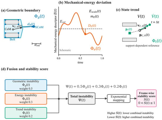
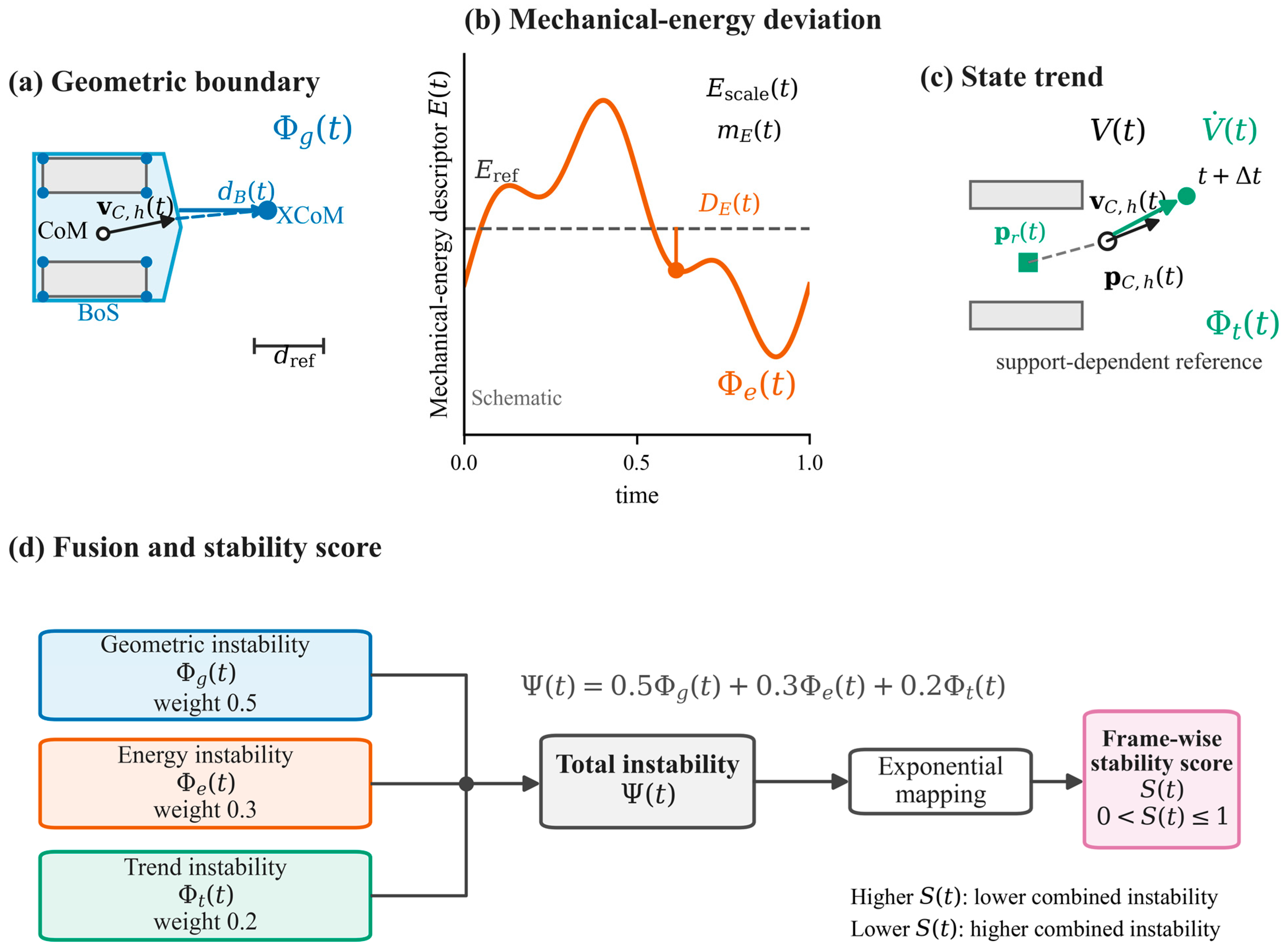
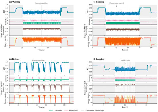
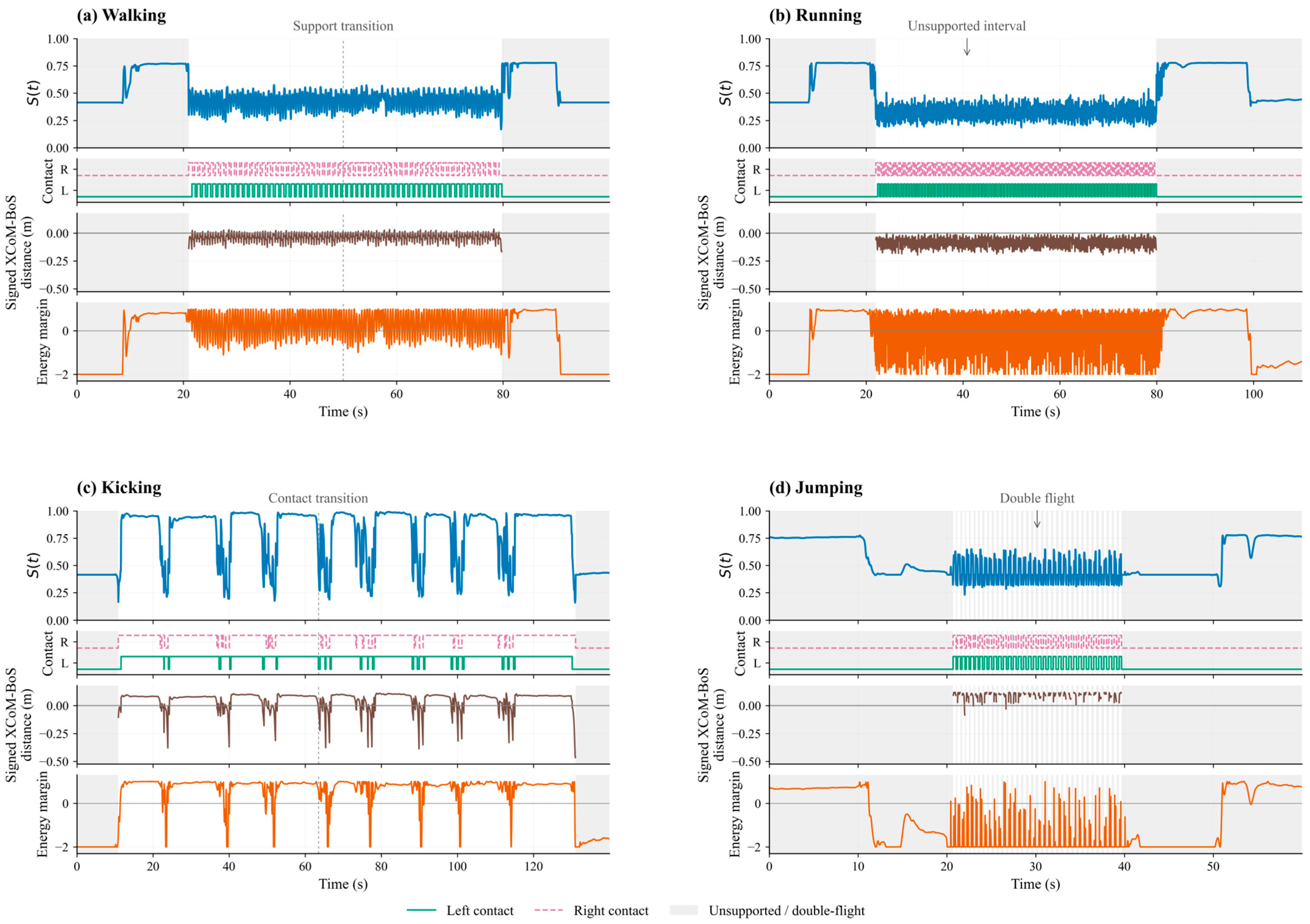
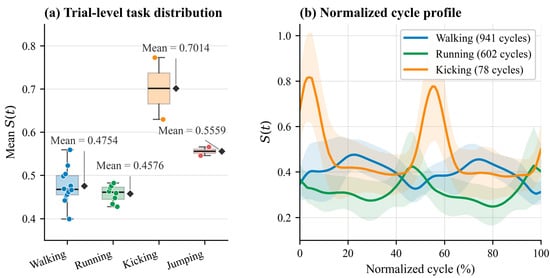
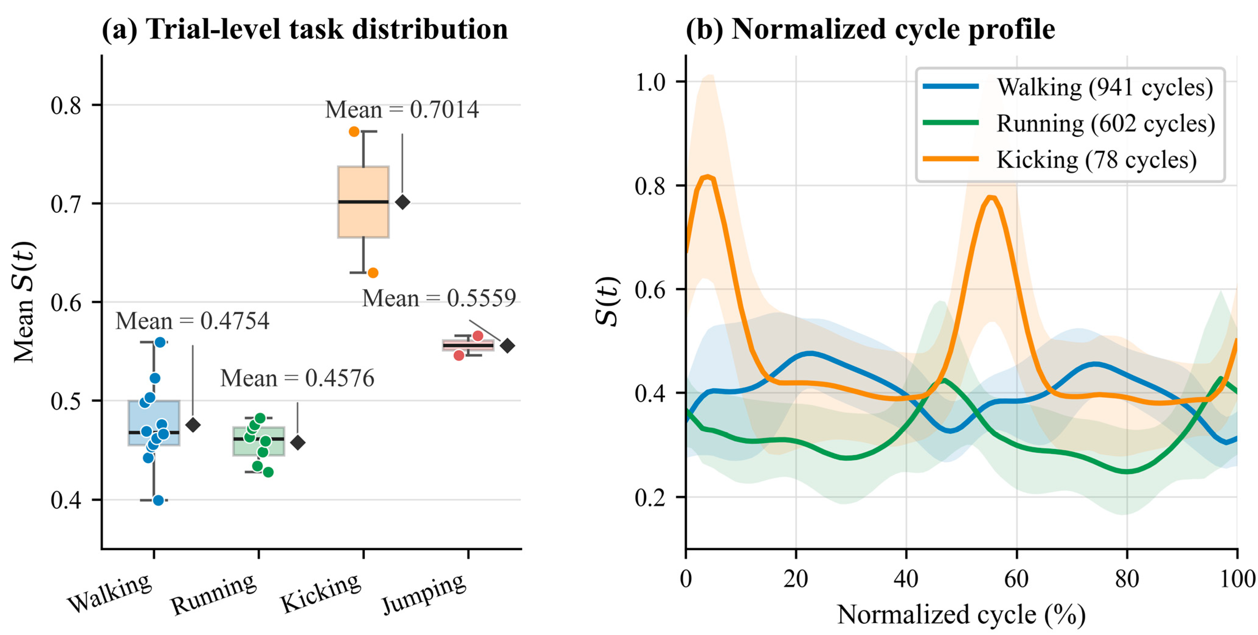
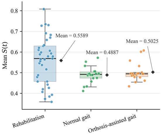
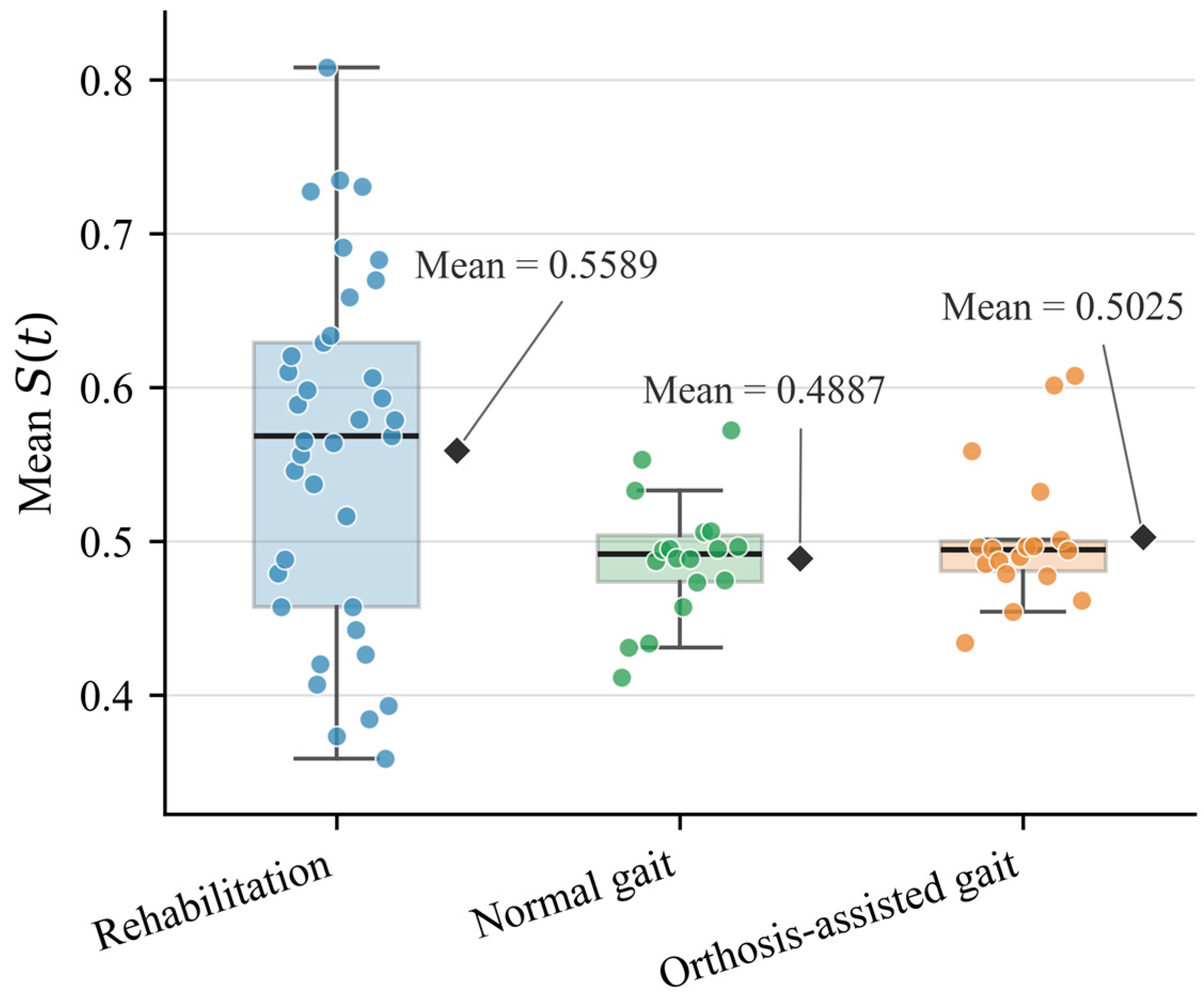

Disclaimer/Publisher’s Note: The statements, opinions and data contained in all publications are solely those of the individual author(s) and contributor(s) and not of MDPI and/or the editor(s). MDPI and/or the editor(s) disclaim responsibility for any injury to people or property resulting from any ideas, methods, instructions or products referred to in the content. |
© 2026 by the authors. Licensee MDPI, Basel, Switzerland. This article is an open access article distributed under the terms and conditions of the Creative Commons Attribution (CC BY) license.