


Abstract
Frequency-shift (FRESH) filtering is a low-compute technique that is deemed an attractive alternative to successive interference cancellation (SIC) algorithms in communication systems that involve resource-constrained devices. FRESH filters exploit the cyclostationary properties of interfering signals by linearly combining the spectrally redundant components of a signal such that they destructively add. Therefore, the performance in terms of bit error rate or mean squared error achievable by a FRESH filter is dependent on the cyclostationarity features exhibited by a signal. Their computationally simple architecture makes FRESH filters well-suited for low-power wireless sensors, whereas their protocol-agnostic operation is appealing to all manners of cognitive radio, making them an excellent component of ad hoc or infrastructure-less networks. This paper surveys the published FRESH filter designs for communication systems and provides empirical data on their performance under a variety of signal-of-interest and interferer signal properties. We contrast various FRESH filter configurations and ways to determine filter coefficients, comparing against a baseline SIC algorithm in terms of cancellation performance.
1. Introduction
Wireless communication signals are occasionally subject to interference from other emissions, which is an event that degrades link performance in terms of throughput and range. Typically, spectral resources are allocated spatially, i.e, frequency bands per location, by entities such as the Federal Communications Commission in the United States. In other words, wireless systems operating in a particular location are allocated a frequency band of their own to prevent interference events from taking place. Although this method is highly effective, problems still tend to arise, with high-profile incidents including concerns over adjacent-channel interference in 2021 between 5G cellular and aircraft altimeters [1], in 2010 between LightSquared’s L-band cellular and GPS [2], and more. Unregulated spectra, such as the 900 MHz, 2.4 GHz, and 5 GHz ISM bands in the USA, allow operation with certain limitations on power level and transmit duration, but importantly, no guarantee of co-channel interference. A common practice in medium-access control in ISM bands is “sense-before-transmit”, which is an effective but imperfect solution. Missed detections by the sensing function or the “hidden terminal problem” result in frequent transmission collisions in these bands, and therefore, loss of data. Cross-technology coexistence in ISM bands, such as between ZigBee and WiFi [3,4], has been studied to mitigate these issues.
Strategies to mitigate co-channel interference have been studied for decades. Broad categories, discussed in-depth later in this article, include simple approaches such as applying a notch filter to narrow-band interference and complex approaches such as adaptive beamforming and successive interference cancellation (SIC). Frequency-shift (FRESH) filters are a curious class of algorithms that exploit the spectral correlation features of interfering signals to cancel the signal. A signal exhibiting spectral correlation (or cyclostationarity) transmits spectrally redundant information, typically in its sidelobes or excess bandwidth (energy transmitted outside of the center frequency plus-or-minus half the symbol rate), which can be manipulated to be coherent with the main lobe and then subtracted. While exploring the scenarios under which these algorithms “work well” and exactly how well they work is one focus of this article, there are a number of immediately apparent benefits to this approach. Firstly, the implementation of these filters is comparable to an adaptive equalizer or a Wiener filter, which already exists in several communications receivers. Secondly, it is highly signal-agnostic in that one architecture can mitigate a variety of interferer types simply by changing some direct digital synthesizer values. Lastly, in the case of a wide-band interferer, there are scenarios wherein the entire bandwidth of the interfering signal need not be digitized for the algorithm to work, which is a requirement of state-of-the-art SIC approaches (or at least typical implementations thereof). These features of FRESH filters are particularly appealing for applications in transceivers of low-SWaP IoT devices or sensor networks nodes, which are discussed in detail later in this article.
This study is motivated by the absence of a comparative study of the performance of these algorithms both analytically as well as on real (i.e., non-simulated) data using lab equipment. This work fills these two gaps in the literature. The contributions of this work are as follows:
- We analyze sweeps over parameters that impact the performance of FRESH filters, using more parameter ranges than what is found in the current literature.
- We provide benchmark performance for several FRESH filter algorithms using software-defined radio (SDR) experiments.
- We provide the computational complexity of an efficient FRESH filter, which we term a “polyphase FRESH filter”.
- We compare FRESH filters to a SIC algorithm in all of the experiments in the analyses listed above.
Throughout this article, linear convolution is denoted as an encircled asterisk ⊛, the complex conjugate is denoted with a superscript asterisk (), vectors are denoted with bold lower-case letters (), matrices are denoted with bold capital letters (), the conjugate (Hermitian) transpose is denoted with a superscript H (), the infinite-time average is denoted with angle braces (), and optional conjugation and negation are denoted with parentheses ( and , respectively).
This article is organized as follows. Section 2 explains the need for interference cancellation and provides a taxonomy of the broad categories of solutions. Section 3 describes how FRESH filters work, first formally and then intuitively, with visual aids. Section 4 presents a literature survey of FRESH filter use cases. Section 5 presents our empirical results for a select set of FRESH filter interference cancellation algorithms, compared against a baseline SIC approach. Section 6 presents similar results using SDRs to observe the impact of more “real” signal impairments. Section 7 presents the results of simulated cases of interference in the 2.4 GHz ISM band, targeting an IEEE 802.15.4 [5] SOI, which is applicable to sensor networks. Section 8 discusses the computational complexity of a communications receiver using FRESH filters, as compared to a SIC-based receiver. Finally, Section 9 concludes the paper with discussion of unexplored application spaces where we envision FRESH filters could make an impact.
2. Interference Mitigation
2.1. Problem Statement
A co-channel interference scenario can be described by a received signal composed of the superposition of a signal-of-interest (SOI) , a noise signal , and an interfering signal . Specifically, the interference scenario is co-channel when the spectral components of and overlap significantly. In a multiple-antenna scenario, is a vector , with one dimension per antenna or analog-to-digital converter. The signals and are broadcast into the vector space through “arrival vectors” and , respectively, which describe the relative magnitude and phase of the signals as observed at each receiver antenna as a function of the azimuth and elevation angles of the sources. While sufficient for this discussion, note that wide-band signals or frequency-selective multipath necessitate changes to this signal model. The vector representation is important when discussing some modern techniques, though most of this article will use the scaler (single-antenna) signal model.
Typically is modeled as a random process, such as Gaussian noise, and mitigation strategies are limited to filtering spectral components that are out of band relative to . For purposes of interference cancellation, or are modeled as having some structure or feature that can be exploited to remove them from , even though they are still fundamentally random processes.
2.2. Successive Interference Cancellation
One of the most researched contemporary interference cancellation techniques is SIC. SIC has garnered volumes of attention due to its relevance to non-orthogonal multiple-access (NOMA)—a promising candidate for future-generation cellular standards [6,7]. For this class of interference cancellation scheme, is a digital communication signal whose structure is known by the receiver. A SIC algorithm will process to estimate as , and coherently subtract it from . Effects of multipath and time-varying effects such as frequency offset or phase drive must be imposed on the estimate [8]. This produces a signal which contains , , and an interference residue signal , such that, if done correctly, .
These techniques require intimate knowledge of . For example, if it is a digital communication signal, at a minimum a modulation scheme is required; however, knowledge of the parameters of any spectrum-shaping filters will improve the cancellation performance [8]. Knowledge of packet types and structure, mixed-modulation information, and forward error correction (FEC) schemes are all examples of aspects of signals that would improve cancellation performance, i.e., reduce .
This technique hinges on a receiver’s ability to correctly demodulate (and possibly apply error correction), meaning that the power of in must be sufficiently larger than and . “Sufficiently large” depends on the sensitivity of the protocol and mode which implements.
2.3. Spatial Filtering
Also known as beam-steering or null-steering, spatial filtering is another highly researched interference mitigation strategy due to its relevance to multiple-input multiple-output (MIMO) systems. These techniques generate a single received signal stream from by computing a weighted combination of the signal from each antenna with coefficients in .
To employ this effectively, and should be known or estimated either using known sequences in and or using direction-finding methods such as MUSIC. Selection of can be performed in a number of ways, such as nulling out by enforcing .
These techniques rely on spatial diversity—in other words, and are not coming from the same direction. Ideally, their arrival vectors are orthogonal, allowing selection of an that results in minimal noise growth. Practically, these techniques often require a calibrated antenna array at the receiver. Blind algorithms may be employed to remove the need for calibration—of note is the the spectral self-coherence restoral (SCORE) algorithm [9,10], which has particular relevance to the topic of this article and will be discussed in Section 4.
3. Frequency Shift Filtering
This section covers relevant background material pertinent to this article. Section 3.1 defines equations and the architecture of a FRESH filter and Section 3.2 discusses solutions for the filter coefficients. Cyclostationary signal modeling is an important fundamental to understanding the operation of FRESH filtering. Appendix A provides relevant notation and background on the principles of cyclostationarity.
3.1. Frequency-Shift Filter Definition
Classic linear time-invariant (LTI) filters can be generalized to linear time-varying filters (LTV), which are filters whose impulse response varies as a function of time. A LTV filter can be specialized to a linear almost-periodic time-varying (LAPTV) filter, which is a filter where the impulse response is an almost-periodic function of time. In other words, the impulse response can be decomposed into a sum of sinusoids. Equations (4) and (5) describe a LAPTV filter, where and are the input and output, respectively, is the time-varying filter impulse response, and are the coefficients associated with the periodic component decomposition with frequency .
After combining the two equations and re-arranging terms, shown in Equation (6), it is apparent that such a filter is equivalent to frequency-shifting the input signal, processing each frequency-shifted “branch” through an LTI filter, and summing the outputs [11]. This describes a linear FRESH filter, as the system response is linear with respect to .
Incorporation of conjugate statistics is done by designing a system that is linear with respect to the tuple —such a system is termed “widely linear”. This is shown in Equation (7), where the system output is the summation of a linear FRESH filter operating on and a linear FRESH filter operating on . The LTI filter coefficients of the conjugate branches are now denoted as and the associated frequencies as . This describes a linear-conjugate-linear (LCL) FRESH filter and a block diagram is illustrated in Figure 1.
Figure 1.
Block diagram of a LCL FRESH filter. FRESH filters generally consist of a set of frequency-shifters, an optional conjugation block, a set of FIRs, and a summation. Adaptation can be employed if a desired response can be streamed in as the filter runs.
3.2. Design Equations and the Cyclic Wiener Filter
For purposes of this article, the goal of a LCL FRESH filter can be concisely stated, from the perspective of the frequency domain, as “linearly combining spectrally redundant components of a signal or its conjugate such that target components of the signal are either amplified, suppressed, or otherwise separated.” As with many equalization problems [12], a desired signal is defined as well as an error signal and the filter coefficients are optimized in the mean-squared error sense. The coefficients can be solved for using either temporal or spectral statistics. The time-domain FRESH filter design equations, transcribed from [11] and originally published in [13], are shown below. We direct the reader to the Chapter 9.3 of the former reference for a brief derivation and Chapter 4 of the latter for more thorough discussion. In the above, B and are the sets of CF for the non-conjugate and conjugate branches, respectively.
The solution for this system of equations is the famous Wiener–Hoph equation, shown in Equation (10) [12]. In this equation, is the concatenation of the filter coefficient of each arm into a column vector, the variable is the concatenation of the tap-delay lines of each filter into a column vector, is the autocorrelation matrix of , and is the cross-correlation between and the desired response d.
The optimal sets of CFs would be the sets that produce the smallest possible mean squared error (MSE), and a FRESH filter using these sets of shifts is termed a Cyclic Wiener Filter (CWF), or the optimum FRESH filter. These sets contain, at most, all possible integer-linear combinations of the CFs present in [11,13,14]. In practice, a CWF may be approximated using least mean squares (LMS), recursive least squares (RLS), or another adaptive algorithm, if training sequences or decision-feedback is available.
4. Literature Review
The work in [13], as discussed in Section 3.2, was foundational to the body of literature, wherein the design equations for filter coefficients were first presented. Reed and Hsi [14] were among the first to theoretically analyze the interference rejection performance of FRESH filters on a variety of wireless communication signals. In [15], the channel capacity of a communications channel subject to second-order cyclostationary noise is derived. Gaussian-distributed noise is used for analytic tractability and therefore the result serves as a lower-bound of the capacity.
There are a number of unique methods of solving for the filter coefficients in a practical scenario. The work in [16] is the earliest work we can find credited with adaptive FRESH filters (referred to as time-dependent adaptive filters therein). In [17,18,19], the constant modulus algorithm (CMA) is extended to FRESH filters, which enables filter blind adaptation for constant modulus signals without the need for pilot sequences or decision feedback. The blind-adaptive FRESH (BA-FRESH) algorithm is presented in [20]—again motivated by use cases where pilots and decision feedback are not available to serve as the desired response. Importantly, the idea of using the input signal itself as the desired signal ( in Section 3.2) is proposed. This idea has been adopted by several FRESH filtering papers, both for interference cancellation and for spectrum sensing [21,22,23,24] and beamforming [9,10,25]. The latter references describe the SCORE algorithm, which uses frequency-shift arms to train beamformer coefficients using a cost function designed to maximize the spectral coherence of the linear combination of each arm.
FRESH filters are commonly studied for interference mitigation of digital communication signals. Early FRESH filter studies on interference mitigation for wireless digital communications focused on co-channel interference of 2G cellular networks [26,27], whereas several newer FRESH filter works consider NOMA [6,28,29]. Single-carrier signals are often focused on, but the time-varying FRESH (TV-FRESH) algorithm considers specifically OFDM signals-of-interest [30,31,32,33] and filter-bank multi-carrier is considered in [34]. FRESH filters are not only limited to exploiting second-order statistics; fourth-order statistics have also been shown to provide some benefit [35].
Noise models in powerline communications (PLC) often follow a cyclostationary model with CFs at harmonics of the alternating current (AC) frequency. Motivated by the IEEE P1901.2 [36] standard, most of the available literature considers removing PLC noise from an OFDM signal. Multi-stage FRESH filters, often using the BA-FRESH algorithm, are found in [37,38,39,40], and sometimes additional measures are taken such as hard-limiting to remove residual noise impulses [41].
Jamming is a form of intentional interference that is used to disrupt a communications system. Depending on the implementation, a jamming waveform can still exhibit cyclostationarity, meaning that the FRESH algorithms may be employed. Interrupted-sampling repeater jammers are mitigated in [42,43], traditional noise jamming is considered in [44], and jamming detection of DSSS signals is considered in [45].
5. Performance Analysis
In this section, we present an analysis of FRESH filtering for interference cancellation. The term “signal-not-of-interest” (SNOI) will be used interchangeably with “interferer”, and “signal-of-interest” (SOI) will refer to the desired signal. Performance of the FRESH filters is compared against a SIC baseline. SIC could, in principle, completely remove the SNOI and therefore should serve as an upper-bound on performance (or a lower-bound on NMSE).
5.1. Metric and Parameters
The performance is quantified as normalized mean squared error (NMSE). The method by which NMSE is calculated is described in the following subsections. Two baselines are presented: standard Wiener filter or RLS equalization and a successive interference cancellation algorithm, serving as performance bounds of the FRESH filter.
It is important to note that improvements in NMSE should not be interpreted as yielding a proportional decline in BER, as NMSE does not consider communications concepts such as matched filtering, decision boundaries, maximum likelihood sequence estimation, impacts of colored noise, etc. To illustrate this point, consider a BPSK constellation with additive complex Gaussian noise. The NMSE of this signal can be easily reduced by removing the quadrature component, which can be modeled as the output of a widely linear filter if the signal and its conjugate are averaged. However, this reduction in the total NMSE does not improve the error rate as the quadrature component runs parallel to the BPSK decision boundary. NMSE is a useful indicator to quickly analyze a scenario; however, communications-specific metrics or analytics should still be leveraged.
The high dimensionality of the problem to be analyzed makes an exhaustive analysis over all parameter combinations intractable. Our approach is to present a “best case” scenario as an upper bound and a “worst case” scenario as a lower bound, followed by several scenarios where the best case has a single signal parameter perturbed. Thus, the impact of a single signal parameter is focused on at a time. The parameters considered are shown in Table 1. Carrier frequency offset (CFO) of the SNOI is the swept parameter for the plots to be presented and each of the 3 relative bandwidths of the SNOI to the SOI are presented using SOI CFs or the SNOI CFs in the FRESH branches. Length-17 filters are selected as the largest filter length with which the data in Section 6 could be processed in a reasonable amount of time, aiming to maximize performance. The symbol rate for the wideband SNOI is selected such that the bandwidth of the SOI fits within one spectral redundancy period of the SNOI so the SOI image at the output of the mixer does not interfere with the the image of the SOI in the 0 Hz arm. The selection of the symbol rate of the narrowband SNOI was similar.
Table 1.
The list of parameters analyzed for impact on FRESH cancellation performance. Where applicable, an asterisk (*) indicates the value used in the best case scenario.
NMSE values using purely analytic means are discussed in this section. These results have been validated by exhibiting consistency with Monte Carlo simulations—because these validation curves overlap the analytic curves, Monte Carlo simulation results are not presented. Each subsection discusses the effects of a different scenario or a signal parameter. A summary of the important observations is provided in Section 5.7.
Analytic results for the MSE of a given scenario are calculated using the following steps. This procedure describes the calculation of the FRESH filter MSE. The same process is repeated, first by setting the frequency shifts to use only a 0 Hz non-conjugate shift to calculate standard Wiener filter MSE, and then by setting the interferer power to 0 to calculate the SIC MSE.
- Compute (or estimate) the limit statistics of the SOI, SNOI, and noise for a symbol rate of 1 Hz, a CFO of 0 Hz, and a power of 1 (analytic expressions for cyclic statistics of linear modulations are trivial [46]; however, those for continuous-phase modulation (e.g., GMSK) are not [47]. As such, statistics for GMSK are estimated using a single, long realization of symbols, which has proven to be sufficient for the variance in the statistical estimate to be low enough to yield consistent results. This was observed over repeated runs of the analysis. Statistics estimated with an insufficiently long realization would produce inconsistent results).
- Transform statistics appropriately for the requested power, frequency offset, symbol rate, etc., to compute and (many of the transformations are trivial; others can be found in Chapter 3 of [11]).
- Solve for the optimal coefficients with the Wiener–Hoph equation .
- Compute MSE as .
This produces bounds the NMSE that one could expect to achieve. There are some assumptions in this process worth noting. First, the SIC receiver is able to perfectly demodulate, de-FEC, and re-synthesize the SNOI. Factors such as the SOI power being high enough to hinder SNOI demodulation [8] or mismatches between pulse shape or window coefficients [48] are not accounted for in this bound. In a similar fashion, the Wiener and FRESH filters perfectly estimate covariance matrices and adaptation noise is zero.
5.2. Best and Worst Case
Results of the best and worst case scenario are shown in Figure 2. To interpret the graph, a lower value is considered better performance, and increasing values on the x-axis indicate less spectral overlap between the two signals. Several important observations can be made. First, the SIC algorithm, in theory, performs better than a FRESH filter. This is because more knowledge of the SNOI is exploited in order to cancel it. These results do not account for imperfections in a receiver’s ability to replicate the SNOI prior to cancellation—this is considered in the next subsection.
Figure 2.
Best and worst case performance. The bandwidth of the SNOI varies from wide (left) to narrow (right). Solid curves indicate “best case” while dashed curves indicate “worst case”. Each color indicates a different interference mitigation algorithm. In the best case, the SOI and SNOI are BPSK modulated with 100% excess bandwidth and the SOI in-band SNR is +20 dB. In the worst case, the SOI and SNOI are QPSK-modulated with 25% excess bandwidth and the SOI’s in-band SNR is +5 dB SNR.
The only instance where the FRESH filter’s performance exceeds that of the SIC algorithm is when the FRESH filter uses frequency shifts corresponding to CFs of the SOI (solid blue curve). Even the asymptotic NMSE as the spectral overlap of the interferer approaches zero is lower than the competing curves. The previous qualifier on using NMSE as the performance metric must be considered here—some of the improvement seen by this curve is akin to removing the quadrature component of a BPSK signal. While this can make interpretation of this specific curve challenging, there are still insights to be gained.
The bandwidth of the interferer is critical for selecting which frequency shifts to use. Narrowband SNOIs tend to be better removed when cyclostationarity of the SOI is exploited. A likely cause for this is the fact that finite-length filters are considered in this analysis and longer filters are needed to achieve sufficient detail to properly manipulate the spectrum of a narrowband signal. This observation is consistent with the design of some FRESH filters discussed in Section 4, such as the example from [49]. Even in the case of comparable-bandwidth SNOI, exploiting CFs of the SNOI in a FRESH filter tends to be a more performant solution.
The FRESH filter’s performance typically suffers as the CFO approaches 0 Hz, regardless of the bandwidth of the SNOI. When conjugate cyclostationarity of the SNOI is exploited, the SOI component in the conjugate branch is treated as an additional interference term. This is a scenario where integer linear combinations of frequency shifts can be used to continue to resolve interference terms, though this is not considered here.
Finally, in the worst case scenario, the FRESH filter fails to attain any meaningful performance gains over the Wiener filter, whereas the SIC algorithm continues to add benefit. The following subsections provide insight into which signal parameters contribute the most to this performance loss.
5.3. Effect of SNOI Modulation
Results of the effects of the SNOI modulation are considered in this subsection. From the perspective of the FRESH filter, the most important difference is the nature of the conjugate cyclostationarity. The BPSK signal has conjugate CFs at harmonics of the symbol rate, centered at twice the CFO; the GMSK signal has conjugate CFs at odd harmonics of the half the symbol rate, centered at twice the CFO, and the QPSK signal has no conjugate cyclostationarity. Performance is compared in Figure 3.
Figure 3.
Impact of SNOI modulation on NMSE. The bandwidth of the SNOI varies from wide (left) to narrow (right). Solid curves indicate a BPSK SNOI, dashed curves indicate a QPSK SNOI, and dot-dashed curves indicate a GMSK SNOI. Each color indicates a different interference mitigation algorithm.
Varying the SNOI modulation only has subtle impacts on the Wiener filter and the FRESH filter using SOI CFs (black and blue curves, respectively)—these impacts are due to the distribution of the spectral energy between BPSK and QPSK (which are identical) and GMSK. The impact on the FRESH filters using SNOI CFs is emphasized. Comparing the BPSK curve (solid red, best case) with the QPSK curve (dashed red) indicates that the QPSK yields strictly worse performance than the BPSK. This is true across all SNOI bandwidths, and is simply due to the fact that QPSK exhibits fewer cyclostationary features to exploit.
Comparing the BPSK curve to the GMSK curve (dash-dotted red) highlights a unique feature, in that using a FRESH filter to cancel a GMSK signal improves performance as the CFO approaches 0 Hz. This is due to the differing location of the conjugate CFs of GMSK signals—there is no double carrier conjugate feature, so the SOI component of the conjugate branches does not overlap and interfere with the SOI in the 0 Hz non-conjugate branch. On the other hand, the SNOI modulation has a relatively minimal impact when the interferer is narrowband. This is consistent with previous observations, particularly that (i) leveraging CFs of wider bandwidth signal is advised, and (ii) varying the SNOI modulation minimally impacts the performance of the FRESH filter using SOI CFs.
5.4. Effect of SOI Modulation
Results of the effects of SOI modulation are considered in this subsection. The same significant differences found when varying this parameter are the same as for varying the SNOI modulation but applied to the SOI instead. The performance is shown in Figure 4. Similar conclusions to those drawn from effects of SNOI modulation can be made here, in that the major effects occur when the SNOI is narrowband.
Figure 4.
Impact of the SOI modulation on NMSE. The bandwidth of the SNOI varies from wide (left) to narrow (right). Solid curves indicate a BPSK SOI, dashed curves indicate a QPSK SOI, and dot-dashed curves indicate a GMSK SOI. Each color indicates a different interference mitigation algorithm.
Comparing the BPSK curve (solid blue) with the QPSK curve (dashed blue) in the narrowband SNOI case again simply indicates that the QPSK SOI yields strictly worse performance than the BPSK SOI. This can be attributed to the same reason as when the SNOI was varied—the lack of conjugate CFs to exploit.
Comparing the BPSK curve to the GMSK curve (dash-dotted blue) in the narrowband SNOI case indicates a similar “dip” in the NMSE of the GMSK SOI near 0 Hz, for the same reason as before—the SOI components of the conjugate branches do not spectrally overlap the SOI in the 0 Hz non-conjugate. Curiously, a GMSK SOI is the only instance where for a narrowband SNOI, the FRESH filter using SNOI CFs (dash-dotted red curve) outperforms the FRESH filter using SOI CFs (dash-dotted blue curve).
5.5. Effect of Excess Bandwidth
Results of the impact of the excess bandwidth of the SOI and SNOI is considered in this subsection. The excess bandwidth of the SOI and SNOI are varied in tandem. This is perhaps one of the most relevant comparisons, as modern communication systems are continually improving their spectral efficiency, which often yields a decrease in the cyclostationarity of signals—the feature that FRESH filters exploit. The results are shown in Figure 5.
Figure 5.
Impact of the excess bandwidth on NMSE. The bandwidth of the SNOI varies from wide (left) to narrow (right). Solid curves indicate a high excess bandwidth of 100% and dashed curves indicate low excess bandwidth of 25%. Each color indicates a different interference mitigation algorithm.
Across all bandwidths, the solid (high excess bandwidth) and dashed (low excess bandwidth) lines exhibit a crossing as CFO increases, where excess bandwidth begins to outperform. This is due to the change in the distribution of the spectral energy of the SNOI—notice that the Wiener filter (black curve) also improves in performance at a lower CFO for the low excess bandwidth scenario.
Consider the FRESH filter using SNOI CFs (solid and dashed red) in the wide bandwidth SNOI case and the FRESH filter using SOI CFs (solid and dashed blue) in the narrow bandwidth SNOI case. The pairs of curves exhibit little difference over the majority of CFO values. Also, consider that as excess bandwidth decreases, the magnitudes of all non-conjugate CFs decrease and the magnitudes of most conjugate CFs decrease, except the double-carrier feature, which is minimally affected. Contrast this observation with two of the previous figures: (1) in Figure 3, using SNOI CFs when the SNOI is QPSK and (2) in Figure 4, using SOI CFs when the SOI is QPSK. Both of these scenarios exhibit more drastic performance degradation when no conjugate cyclostationarity is leveraged. This highlights the importance of using conjugate cyclostationarity when available.
5.6. Effect of SNR
Results of the effect of the SOI SNR are captured in Figure 6. The relative power of the SNOI to the SOI is held constant between the two scenarios.
Figure 6.
Impact of SOI SNR on NMSE. The bandwidth of the SNOI varies from wide (left) to narrow (right). Solid curves indicate a high SNR of +20 dB and dashed curves indicate low SNR of +5 dB. Each color indicates a different interference mitigation algorithm.
The results indicate that the primary effect of SNR is on asymptotic NMSE as the CFO of the SNOI increases. This applies across all bandwidths or selected CFs. Although SNR appears to be the largest contributing factor to the high difference in NMSE between the best- and worst- case scenarios in Figure 2, the same trends on when different configurations work better than others remain consistent with low SNR.
5.7. Summary of Analytic Results
It comes as no surprise that SNR is the most limiting factor in the resulting NMSE of each algorithm. The considered scenarios suggest that for wideband and moderate-bandwidth SNOI, the SNOI CFs should be prioritized when designing the FRESH filter. Conversely, for narrowband SNOI, CFs of the SOI should be prioritized. Because of this, the modulation of the SNOI has the most influence on performance in the wideband SNOI case and the modulation of the SOI is the most influential on performance in the narrowband SNOI case. Using both sets of CFs is, of course, an option; however, the computation complexity for solving for the filter coefficients can grow quickly as the number of accounted-for frequency shifts increases.
Further, conjugate CFs typically yield better NMSE improvement than non-conjugate. Conjugate CFs of the SNOI, in particular, are highly effective; however, the impact of conjugate CFs of the SOI on more relevant communications metrics, such as BER, are less than what this analysis suggests. This is explored in the next section.
6. Software-Defined Radio Results
6.1. Experiment Setup
Three Ettus USRP X310s are used to test interference cancellation performance on real data. Three SDRs are placed on a bench a couple of feet apart. The sample rate of the radios is 1 MHz and the same relative symbol rate numbers from Section 5 are used, so the SOI has a symbol rate of 62.5 kHz, the wideband SNOI has a symbol rate of 250 kHz, and the narrowband SNOI has a symbol rate of 15.6 kHz. The signals are all “textbook modulations”, so they are constant-rate, constant-modulation BPSK, QPSK, or GMSK. The carrier frequency is tuned to 3.1 GHz. No significant multipath is expected. Two SDRs transmit known signals co-channel with one another, while the third SDR receives their signals. The signal strength of each transmitter to the receiver and carrier frequency errors are calibrated before data collection begins. For each scenario, the frequency offset of the interferer is swept in discrete steps until the signals no longer overlap. The length of the sample vectors collected is 500,000 RF samples, or SOI data symbols, for each frequency offset value. In post-processing, the received signal is correlated against the known transmitted sequences in order to identify when the transmissions start to determine what the appropriate desired response is for each cancellation algorithm.
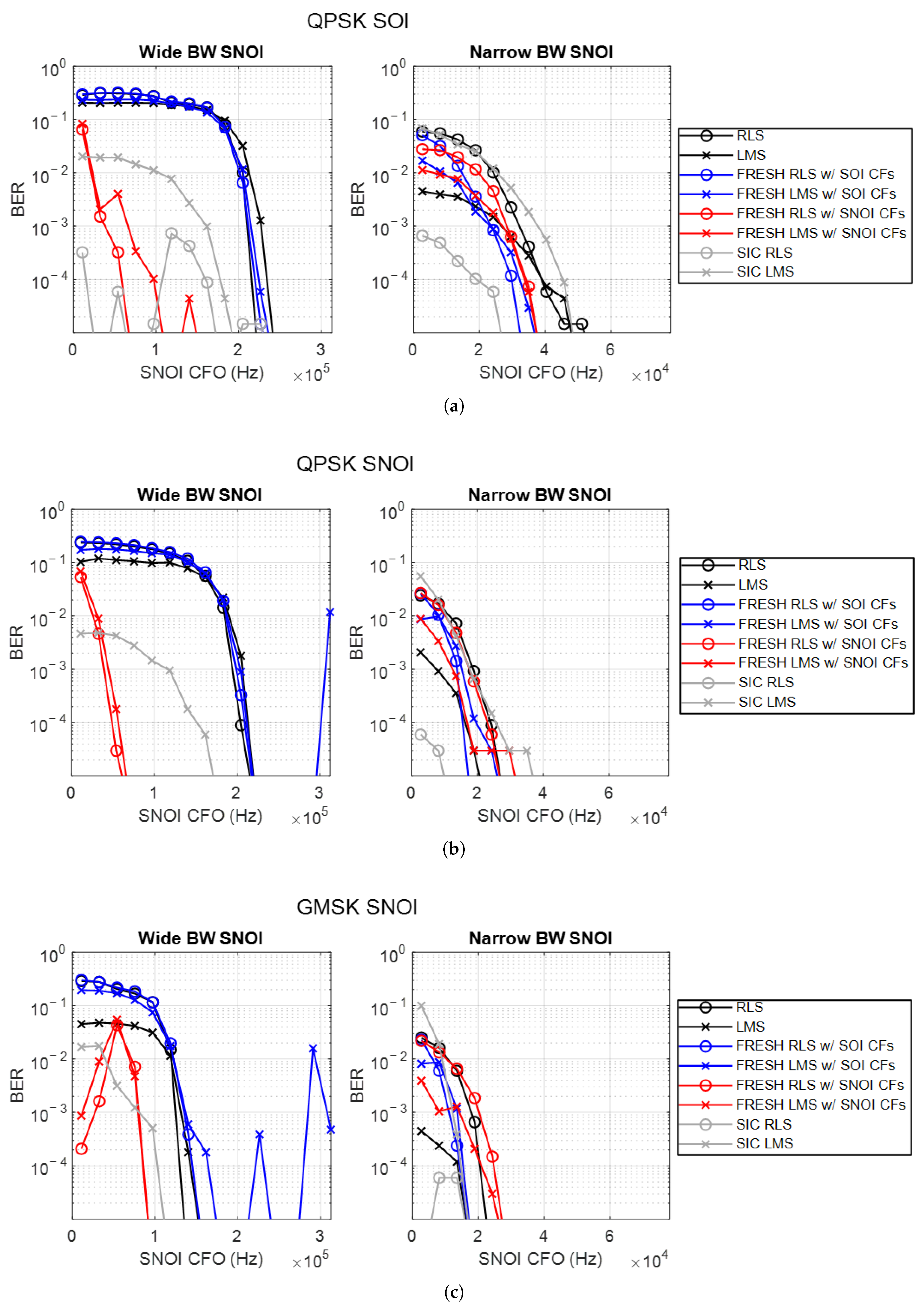
The best case and the GMSK SOI scenarios are considered as they provide the most insight in addition to what was discussed in the previous section. Additional results are presented in Appendix B, providing supplementary validation evidence yet little additional insight into the behavior of FRESH filters. This section is intended to corroborate the previous analytic results with real data and also to consider algorithms whose NMSE is not as easily estimated analytically. Real imperfections impact these results, including unknown oscillator frequency bias and noise and adaptation noise. The SIC algorithm must accurately estimate the SNOI in the presence of the SOI; however, to this end, the SOI is an interference term and will cause an imperfect estimate—the impact of this is observed. Several equalization or interference mitigation algorithms are considered, noted below. Bit error rate (BER) measurements are noted for RLS, LMS SIC with RLS and LMS adaptation, and FRESH RLS and LMS when the SOI is BPSK or QPSK.
- RLS and LMS equalizers.
- FRESH RLS and LMS using SOI CFs.
- FRESH RLS and LMS using SNOI CFs.
- BA-FRESH [50] using SOI CFs.
- FRESH CMA [17,18] using SOI CFs when the SOI is GMSK.
- FRESH CMA using SNOI CFs when the SOI is GMSK.
- SIC [8] with RLS and LMS adaptation.
Adaptive algorithms were chosen to compensate for inaccuracies or changes in the cycle frequencies of the SOI and SNOI. Oscillator frequencies and phases driving the carrier and the sample clock will differ between each SDR and therefore the cycle frequencies will differ from what is expected. This is especially noticeable when conjugate CFs are used, as both frequency drift and phase noise could change the phase or frequency of the conjugate CFs in a short time, relative to a sample clock. Adaptive algorithms have been used to combat this [51,52] and were therefore selected for this experiment. The SIC algorithm is similar to that presented in [8]. A summary of the algorithm is enumerated below and a more detailed description can be found in Section 8.
- A receiver (synchronization, equalization, error correction) is run for the SNOI.
- The SNOI is re-synthesized without impairments or additive noise or interference.
- The measured carrier frequency offset, sample clock drift, and multipath are all applied to the re-synthesized SNOI.
- The re-synthesized, distorted SNOI is subtracted from the received signal.
- A receiver is run for the SOI on the residue of this subtraction.
The LMS adaptation is normalized by the input vector norm for ease of setting the adaptation constant to not be a function of the signal magnitude [12,22]. The LMS adaptation constant of 0.3 and an RLS forgetting factor of 0.95 are used in these results. The values were determined through parameter sweeps and were optimal for our test setup, with these signal levels and approximately optimized performance used for each RLS-based or LMS-based algorithm. A generalized performance analysis remains untested.
BA-FRESH and FRESH CMA are blind algorithms and therefore are expected to perform worse than the others—in fact, FRESH CMA is not guaranteed to converge in all scenarios. Standard CMA was also tested but never converged, likely due to the low SINR of the SOI, and was therefore omitted from the results. Blind algorithms come with the benefit of not needing to provide a desired response to the adaptation algorithm to achieve some level of interference reduction. The NMSE of the blind algorithms must be calculated on a per-block basis because there is no guarantee that the recovered signal is perfectly coherent with the desired response due to residual frequency error and phase noise. The MSE of the blind algorithms is computed over K blocks of length-M segments of the received signal data where the received SOI component is approximately coherent within each block, i.e., accumulated clock or oscillator errors are negligible. Within each block, an estimate of the cross-correlation between the desired response and the filter output is taken, described by Equation (11). This is used to scale each block of filter output to best match the desired response such that their difference approximates the MSE within that block. This computation is described in Equations (11) and (12).
6.2. Best Case
This section presents the results for the best case scenario using the measured data. Figure 7 presents a comparison of NMSE and BER. The analytic curves (dashed) should serve as lower-bound estimates for the measured (solid) curves of the same color. There are few instances where these curves are exceeded in NMSE. Two causes may contribute to this, including the following: (1) imperfect SNR estimation of the measured data and (2) differences in how the MSE is calculated between analytic and measured. The analytic and measured curves of the same color being close to one another is the desired result. BER curves for this scenario are also shown in the figure. Supplemental NMSE and BER results can be found in Appendix B. Note that in the BER graphs, no CFO curve is present, indicating that no bit errors were observed.
Figure 7.
Performance of the best case scenario using SDR data in terms of (a) NMSE and (b) BER as a function of carrier frequency offset of the SNOI. A total of 32k bits are used to calculate the bit error rate. The bandwidth of the SNOI varies from wide (left) to narrow (right). Each color indicates a different interference mitigation algorithm. BA-FRESH NMSE under the wide bandwidth SNOI is greater than 0 dB and not seen on the graph; similarly, SIC RLS BER for the wide bandwidth SNOI is less than and not seen. A total of 32,768 bits were processed, so no less than approximately BER can be resolved.
A clear observation is the difference of approximately 8 to 10 dB in NMSE between the measured and analytic SIC algorithm (gray curve). We attribute this to the imperfect estimate of the SNOI prior to cancellation due to the SOI being an interference term for this function. This is a well-known phenomena and could certainly be improved upon using iterative or joint detection algorithms, e.g., [53]. While the performance of the SIC algorithm still exceeds the RLS, LMS, and Wiener filters (black curves), this highlights a potential benefit of the FRESH filters, specifically, yielding high excess bandwidth signals with a power level that is modestly higher than the SOI. This observation is consistent in all of our SDR experiments.
The FRESH filter-measured curves (blue and red solid) exhibit good alignment with the analytic curves (blue and red dashed), staying within approximately 3 dB difference. The primary suspected source of performance difference (apart from SNR estimation errors) is the adaptation noise used by the LMS and RLS algorithm, which uses a history of sample estimate errors or estimates of correlation matrices to derive the filter coefficients, rather than perfect knowledge thereof. This is, however, is a necessary concession due to “model errors” introduced by the SDR—namely, imperfect estimates of the CFs [51,52] and frequency drift, which primarily impacts conjugate CFs.
Consider the NMSE in the narrowband SNOI scenario where the FRESH filter uses SOI CFs. The NMSE of this FRESH filter almost exclusively surpasses that of the SIC algorithm. However, the opposite is true for the BER curve. The FRESH filters using SOI CFs are exclusively surpassed by the SIC algorithm using RLS and are comparable to the SIC algorithm using LMS. This reinforces our cautionary note that using conjugate CFs of the SOI may appear to make a FRESH filter perform better from the perspective of NMSE, while a more useful metric like BER does not see as much benefit.
The frequency drift of this setup was measured to be approximately 500 Hz, so the tracking algorithms were able to correct for at least 500 Hz of CF error using conjugate CFs with a sample rate of 1 MHz (a normalized CF error of 0.0005).
6.3. Effect of QPSK SOI Modulation
Results of the QPSK SOI scenario using the measured data are presented in this section. Figure 8 provides a comparison of NMSE and BER.
Figure 8.
Performance of the QPSK SOI scenario using SDR data in terms of (a) NMSE and (b) BER. A total of 65,536 bits were processed, so no less than approximately BER can be resolved.
The prime takeaway from this comparison is the similarity of the “cross-over” points between the FRESH filter curves and the SIC curves; under conditions where the NMSE of one algorithm is better, it tends to perform better in terms of BER as well. Conjugate CFs of a QPSK SOI cannot be used (as there are none), and the FRESH filter using SOI CFs does not give a false impression of over-performing from the perspective of NMSE.
6.4. Effect of GMSK SOI Modulation
The results of the GMSK SOI scenario using the measured data are presented in this section. The FRESH CMA algorithm is applicable in this case, and can be used to exploit the knowledge that the SOI has a constant modulus to cancel the SNOI. Results of this scenario are presented in Figure 9.
Figure 9.
Performance when the SNOI modulation is GMSK as a function of carrier frequency offset of the SNOI. The bandwidth of the SNOI varies from wide (left) to narrow (right). Each color indicates a different interference mitigation algorithm, including FRESH CMA algorithm, which can be used for a constant-modulus SOI. A total of 32,768 bits were processed, so no less than approximately BER can be resolved.
The initialization of CMA algorithms is an important factor to achieving the desirable performance. The non-linearity (a magnitude squared operation) in the algorithm will produce cross-products of the noise terms, resulting in an SNR loss that is inversely proportional to the input SNR—a phenomena often termed “squaring loss” [54]. It is therefore desirable to have the coefficients initialized to maximize the SNR before this non-linearity before the adaptation is able to optimize the weight vector. We initialize the filter of the 0 Hz non-conjugate arm to a low-pass filter matching the bandwidth of the SOI and the other coefficients to a value of 0. This is a heuristic approach to initialization, with the design goal of removing as much interference as possible at the initial time step prior to the non-linearity in the adaptation step, asserting a priori knowledge only on the SOI bandwidth. The recommended approach for conventional CMA is to initialize all values of the equalization filter to a value of 0 except for the reference tap to a value of 1 [12]. Conversely, for FRESH CMA specifically, A. Jauhar [18] found that initializing filter taps for the 0 Hz non-conjugate arm to a value of 1 and the rest to a value of 0 achieved the best results. With our dataset, our heuristic converged the most consistently and only failed to converge in cases where the spectral overlap was severe, where the other approaches failed as well. A more rigorous approach to FRESH CMA initialization stands as an open question.
The key observation is that the performance of the FRESH CMA algorithms is highly sensitive to spectral overlap, which directly impacts the SINR at the output of the initialized filters. The FRESH CMA using SOI CFs (green curve) begins converging at the frequency offset where the Wiener filter (black curve) can attain a NMSE of −8 to −10 dB. For the given scenario, one can argue that an SNR of approximately +8 to +10 dB is required for convergence. The FRESH CMA using SNOI CFs (dark blue curve) only converges in the narrowband SNOI case and even in this case, its performance is worse than the FRESH CMA using SOI CFs. This is consistent with the observation in Section 5.4 where the GMSK SOI under a narrowband interferer is better rejected using SOI CFs.
6.5. Summary of Software-Defined Radio Results
This section has corroborated the results of the analytic analysis. An implementation loss of approximately 2 to 3 dB between the measured and analytic NMSE is observed, which is consistent with what a practical system would be expected to exhibit. Blind adaptation algorithms are indeed shown to have some improvement in NMSE; however, are severely limited when the SINR of the SOI is particularly degraded. A more focused study on how signal parameters affect these algorithms is warranted.
7. ISM Band Application
In this section we present simulation results of applying a FRESH filter to a receiver for an IEEE 802.15.4 receiver, used in low-power devices that may benefit from computationally light algorithms. An IEEE 802.15.4 (SOI) network-operating co-channel with an IEEE 802.11 (SNOI) network is considered. Both IEEE 802.11b (“DSSS SNOI”) and 802.11n (“OFDM SNOI”) variants are considered. A no-multipath model and a two-ray multipath model with a maximum delay spread of 3.2 microseconds are considered. These models represent open environment and indoor multipath environments, respectively.
An 802.15.4 receiver may have a sample rate around 4 MHz. The non-conjugate CFs of the DSSS SNOI occur at harmonics of 1 MHz and those of the OFDM SNOI occur at harmonics of 250 kHz, which are both “captured” by the sampled bandwidth of the receiver. Therefore, there is no need for the SOI receiver to sample the entire bandwidth of the SNOI to achieve some degree of cancellation—it just needs to sample high enough to capture the desired spectral redundancy (higher than the CFs), which cannot be said for conventional SIC algorithms.
Based on observations from Section 5 and Section 6, because the SNOIs have wider bandwidth than the SOI, CFs of the SNOI are used. For the DSSS SNOI, non-conjugate frequency shifts of MHz are used, and for the OFDM SNOI, non-conjugate frequency shifts of and kHz are used. The sample rate is 4 MHz. The SNOI signals operate on 802.11 channel 1 and the SOI operates on 802.15.4 channel 13, resulting in a carrier frequency offset of 3 MHz. Filter lengths of 5 and 17 are tested and the results are shown in Figure 10.
Figure 10.
Results of the simulated interference cancellation results in the ISM band. Length-5 (a) and length-17 (b) filters are simulated. Each color represents a different SNR of the SNOI; solid lines and dashed lines indicate FRESH filter and Wiener filter performance, respectively; and circle and ‘x’ markers indicate no multipath and with multipath, respectively.
Considering the DSSS SNOI, when no multipath is present (the curves with ‘o’ markers), little benefit is seen with the FRESH filter (solid curves) over the Wiener filter (dashed curves) when increasing the filter size from 5 to 17. However, considerable gain is seen over the Wiener filter when the SNOI SNR is 10 and 20 dB, where approximately 7 dB of cancellation gain is observed at BER. Similar results are observed when multipath is present, with a gain of approximately 4 dB.
Considering the OFDM SNOI, little gain is seen, even with the length-17 filters. The likely reason for this is that the spectral redundancy of an OFDM signal overlaps with adjacent subcarriers, so it is challenging or infeasible to use the spectral redundancy of a subcarrier to suppress it without adding the adjacent subcarriers as additional interference terms. This is a similar observation to the effect of reduced excess bandwidth in Section 5. Nonetheless, using CFs of an OFDM signal in a FRESH filter does not provide as much gain as standard single-carrier signals.
8. Complexity Analysis
Thus far in this article, the desired response is assumed to be known for optimal cancellation, serving as an approximation of performance bounds. In this section, a practical diagram for a SIC-based receiver and a FRESH-filter-based receiver are presented. These diagrams are based off of the synchronization loop diagrams presented in Chapter 10 of [55]. These diagrams are used as a reference to estimate the complexity of each approach in terms of floating point operations per unit of time.
8.1. SIC Receiver
A diagram of the SIC-based receiver is presented in Figure 11. There are three main components: a receiver for the SNOI, a re-synthesis of the SNOI with impairments to match the received signal, and a receiver for the SOI. This is an adaption of the system presented in [8], tailored for a single-carrier modulation format. This inherently assumes that the SNOI has a higher power than the SOI, which is the case in power-domain NOMA and reflects the experiments in Section 6. Optimally, the processed signal for the SNOI would also undergo FEC decoding before re-synthesizing the SNOI for cancellation. This has two crucial implications: first, it adds to the complexity and second, it adds latency to recovering the SOI, since the cancellation needs to wait for the SNOI to finish transmitting (if block codes or interleavers are used). FEC is not considered herein due to the vast number of schemes that could be employed.
Figure 11.
Diagram of a receiver of a weak communications signal using successive interference cancellation. An SNOI receiver first estimates the transmitted SNOI, which is then re-synthesized and distorted to match the input to cancel, so the SOI can then be recovered.
The “SNOI receiver” section runs at the symbol rate of the SNOI. Note that the “SOI receiver” is the same as the SNOI receiver, running at the symbol rate of the SOI. The “Synthesize SNOI” blocks run at the oversampled SOI rate, where is the oversampling ratio (the sample rate relative to the symbol rate). The number of complex floating point operations (FLOPs) for each block is described in Table 2 below. The product of the symbol rate and the summation of these terms is the complexity of the SNOI receiver in FLOPs per second. In the table, is the number of coefficients in a matched filter, is the number of coefficients in an equalization filter, is the number of iterations in a COorinate Rotation Digital Computer (CORDIC), and is a symbol rate.
Table 2.
Description and FLOP count for each block in the SIC receiver.
8.2. FRESH Filter Receiver
A diagram of the FRESH-filter-based receiver is presented in Figure 12. There is modest novelty in this design, which is the introduction of a decimation stage in between the frequency-shifters and the FIRs in the FRESH filter. This allows downstream processing to happen at the critically sampled symbol rate, reducing FLOPs per second. We simply call this design a “polyphase FRESH filter”.
Figure 12.
Diagram of a receiver of a communications signal using a multirate FRESH filter, where the output of each FRESH mixer is decimated before being processed by the FRESH FIR. No intermediate SNOI estimate is computed with this algorithm.
The complexity of the carrier tracking, symbol phase tracking, and detector are the same as described for the SIC receiver, operating now at the SOI symbol rate. The complexity of the blocks in the multirate FRESH filter are described in Table 3 below.
Table 3.
Description and FLOP count for each block in the multirate FRESH receiver.
8.3. Floating-Point Operations Analysis
Graphs indicating the computation complexity of the various receiver algorithms are presented in Figure 13. Matched filter lengths of 16 and oversampling ratios of 4 are used, as these are reasonable values in a typical receiver. The x-axis indicates the length of the FIR in each equalizer. FRESH filters with 3, 5, and 6 frequency-shift arms are presented, as these would be applicable to BPSK, GMSK, and QPSK, respectively (though fewer can always be employed). This means that for FRESH filters, the total number of coefficients is . Definitions of narrow and wideband are the same as in the previous sections. The software used to produce the results in this section is available upon request.
Figure 13.
Complexity of the SIC and FRESH filter receivers as a function of the adaptive filter lengths. Complexity is measured in floating point operations per SOI symbol period. Blue curves indicate SIC, black curves indicate standard equalizers, and red curves indicate FRESH filters. Different markers on the red curves indicate a different number of FRESH arms used. Dashed lines indicate RLS adaptation while solid lines indicate LMS adaptation.
The FRESH filter complexity is invariant to the bandwidth of the SNOI—the complexity of the SIC curves is what noticeably changes between the narrow and wide BW graphs. When using RLS adaptation, the driver of complexity of FRESH filters is the term. This indeed causes the complexity to exceed that of the SIC algorithm in some cases: in the wide BW interferer scenario, only a few frequency-shift arms constitute a complexity benefit to the FRESH filter; in the narrowband interferer scenario, the FRESH filter is always more complex than the SIC algorithm. This again indicates that FRESH filters are best suited to wideband interference scenarios. Conversely, using LMS adaptation highlights more opportunity for computation savings using a FRESH filter with a wideband SNOI. The same is true with a narrow BW SNOI, though it still only surpasses the SIC algorithm with its small number of frequency-shift arms.
Consider the IEEE 802.15.4 receiver in Section 7. Length-5 filters with three non-conjugate arms achieve considerable interference mitigation against the 802.11b signal. The chipping rate of the SOI is 1 MHz. Referencing the wideband SNOI curves in Figure 13 and the rough energy costs for 45 nm ASIC technology in [56] for 32-bit integer additions (0.1 pJ) and multiplications (3.1 pJ), a rough power estimate of 1.62 mW can be derived to run the FRESH filter.
8.4. Cycle Frequency Estimation
While this article has focused on the mechanisms of the FRESH filter, it is worth noting the process of selecting what frequencies to use to parameterize the FRESH filter. Cycle detectors can be easily constructed by estimating the (conjugate) cyclic autocorrelation function (see Appendix A). This can be performed in a highly sensitive, computationally intense manner with an exhaustive spectral coherence search, e.g., [57], or in a manner as simple as as a peak-finding function in a single, long FFT of a (conjugate) lag product waveform [58]. Performance of cycle detectors has been extensively studied in the literature [59].
If conjugate CFs of either the SOI or SNOI are used in a FRESH filter and the frequency offset of the signal may have drifted far enough such that the tracking algorithms can no longer correct, then they may need to be re-estimated. If the CFs need to be estimated, the computationally simple approach is peak selection of the (conjugate) cyclic autocorrelation function, which has complexity where N is the number of samples used. This is particularly appropriate when the SNOI, for which the CFs need to be estimated, is of high SNR. The energy required, using the same joules per FLOP as before, would be on the order of tens of nJ using 1024 samples up to single-digit μJ using 16k samples. The resolution of the cycle frequency accuracy of an estimator is , where is the sampling frequency, or simply normalized frequency. Referencing the 500 Hz number from Section 6, 2048 samples would satisfy this requirement from the perspective of tolerable CF error.
8.5. Summary of Complexity Analysis
We have identified the configurations under which a FRESH filter has computational advantages compared to a SIC algorithm. The FRESH filter complexity grows with ; therefore, keeping either and to a minimum is what will allow these benefits to be realized. Furthermore, it is shown that wider bandwidth SNOIs will also cause the complexity of the FRESH filter to become more favorable. Configurations under specific signal conditions where the FRESH filter will be operating must be analyzed to understand if this tradeoff is appropriate. This section used FLOPs per unit of time as the metric for complexity; however, several factors have been omitted for the sake of keeping the parameter space small. For example, FEC of the SNOI is not considered; if the BW between the SNOI and SOI is great, then additional resampling stages may need to be added; if the bandwidth of the SNOI is much greater than that of the SOI then RF bandwidths and ADC clock rates may need to be considered.
9. Discussion
FRESH filtering is a computationally simple yet effective method to mitigate interference under proper circumstances, requiring little a priori knowledge about the interferer to operate. Our work has highlighted the impact that varying signal parameters has on the performance and complexity of FRESH filters, with a focus on single-carrier digital communication signals. The intractably large parameter space was addressed by focusing of the effects of individual parameters. Several works have studied the benefits of these algorithms; however, it is rare that broad parameter sweeps are performed. In [60], the author cites a number of open questions—one we would like to highlight is (transcribed directly from the reference) “For a given signal and interference scenario, how do we pick good frequency shifts? We’d like an algorithm that can find a minimal set of shifts that provides output NMSE to within X dB of the cyclic Wiener filter for the scenario.” Given the wide parameter space, this is incredibly challenging; maybe sub-optimal, greedy, or heuristic algorithms could still be successful. Our NMSE and BER experiments have only considered RLS and LMS adaptation with filter lengths of 17, which is shown in the complexity analysis to be computationally inferior to a SIC algorithm. An exercise could be performed where the number of filter coefficients for each competing algorithm could be optimized under a specific scenario and the complexity and performance of each implementation weighed. Further, we have assumed that the number of coefficients in each FRESH arm is the same, though this need not be the case and could be inspected in future work. We have reported approximate performance bounds given that the SNOI and SOI sequences are known for training the filter coefficients; the specific receiver implementations presented in Section 8 have not been compared in terms of performance. Finally, frequency-selective multipath was not considered, either in the analytic models in Section 5 and a multipath-light environment was used for the experiment in Section 6. This could be rigorously studied in future work under a variety of channel conditions.
Three application spaces where we see fruitful research opportunity include satellite communications (SATCOM), internet-of-things (IoT), and cognitive radio (CR). SATCOM frequency allocations are often made with guard bands of sufficient width to allow signals to “roll off” sufficiently to not interfere with adjacent channels. A possible capacity improvement could be made if these guard bands were reduced and adjacent channel interference were allowed to happen, under the assumption that receivers are sampling at a sufficiently high rate and employing a linear FRESH filter to suppress the adjacent channel interference. The linear FRESH filter would need two non-conjugate arms: and , where is the symbol rate of the adjacent channel at a lower frequency and is that of the adjacent channel at the higher frequencies. These frequency correspond to shift values that would cancel each adjacent channel with one frequency shift arm for each. This could allow channels to be wider or the inclusion of additional channels in the same finite bandwidth, thereby increasing the overall capacity.
A CR network operating in an underlay paradigm may find itself in a situation where it needs to mitigate co-channel interference from a variety of primary users (PU), some of which may be unknown to the CR. The lack of intimate knowledge of the PU signal is not a problem for employing a FRESH filter interference mitigation strategy, as only the cycle frequencies of the PU signals are needed, which are easy to measure using observations of the PU signals. Further, the generic structure of the FRESH filter enables it to be compatible with a variety of possible environments with diverse signal types. Based on the different type of PU signal, the CR may decide to select a frequency and bandwidth where the FRESH filter will provide the most benefit—lessons from Section 5 are directly applicable to this use case.
Author Contributions
Conceptualization, S.F.; Methodology, S.F.; Software, S.F.; Investigation, S.F.; Writing—original draft, S.F.; Writing—review and editing, M.Y.; Visualization, S.F.; Supervision, M.Y. All authors have read and agreed to the published version of the manuscript.
Funding
This research was funded in part by The Johns Hopkins University Applied Physics Laboratory: No grant number associated.
Data Availability Statement
The data presented in this study are available on request from the corresponding author due to employer approval requirements.
Acknowledgments
The authors would like to thank Chad Spooner and Marilynn Wylie for their guidance in development of the software used to generate the analytic performance curves. The authors would also like to thank Zachary Hicks and Austin Au-Yeung for their support in initial development of FRESH LMS and BA-FRESH, respectively. The authors would finally like to thank The Johns Hopkins University Applied Physics Laboratory for funding initial explorations of FRESH filters.
Conflicts of Interest
The authors declare no conflicts of interest.
Appendix A. Primer on Cyclostationarity
This section introduces the fundamental concepts underlying the cyclostationary signal model. The reader is referred to [11] for a comprehensive review of the topic. Signals discussed herein are complex-valued and zero-mean (zero-mean means that the infinite time average and the ensemble expectation, which is possibly a time-varying function, are both zero. Non-zero mean signals, where the stochastic expectation of the signal has additive sinusoids, are termed first-order cyclostationary signals. The equations become slightly burdensome for non-zero-mean signals yet the core concepts still apply in both cases—as such, we assume zero-mean signals in favor of simplicity). When discussing complex-valued random processes, non-conjugate and conjugate statistics are needed to fully describe its second-order statistics. Both non-conjugate and conjugate statistics are compactly represented using optional conjugation and negation . In this article, all optional conjugations and negations are either jointly present or jointly omitted from an equation. Using conventional nomenclature (albeit non-intuitive), when the optional conjugations are present, the equation is said to describes non-conjugate statistics; conversely when they are omitted, the equation is said to describes conjugate statistics (in the literature on cyclostationarity, a function name, such as the autocorrelation function is often preceded by the word “(conjugate)” in parentheses to acknowledge the presence of optional conjugation in the equation. We choose not to include this as it is generally implied throughout this article).
A cyclostationary random process or signal is one whose statistical properties are almost-periodic functions of time. In the stochastic sense, a second-order cyclostationary signal has the following property:
where
is the cyclic autocorrelation function (CAF) at cycle frequency (CF) and is the set of CFs where exhibits second-order cyclostationarity. In other words, in the autocorrelation function at lag , the CAF is the Fourier coefficient associated with the additive sinusoid with frequency . In the fraction-of-time (FOT) sense (the FOT random process model is a statistical model where stochastic properties are estimated from a single realization of a random process rather than an ensemble), the equations are as follows:
where
The CAF is a temporal moment function, which has a dual spectral moment function, the spectral correlation function (SCF), or the cyclic spectrum. The CAF and SCF are related via the Cyclic Wiener Theorem, or the Gardner relation:
Note the similarity in form to the Wiener–Khintchine Theorem, which relates autocorrelation to spectral density for wide-sense stationary signals. As the name implies, the SCF describes spectral components of a signal which are statistically correlated—in other words, the SCF describes redundant information in a signal’s spectrum. True to this concept and pertinent to this article is the relation between the SCF and the short-time Fourier transform (STFT) of the signal,
where
is the STFT of with center-time t and window duration T. Finally, a pair of signals and are said to be jointly cyclostationary if their cross-CAF or cross-SCF are non-zero for some CF, lag, and spectral frequency. The set of CFs where and exhibit joint cyclostationarity is denoted as . These functions are simple generalizations of the CAF and SCF. The functions in the stochastic sense are shown below.
Digital communication signals are a notable class of cyclostationary signals. For many “textbook” signal models (e.g., phase-shift keying (PSK), quadrature-amplitude modulation (QAM), minimum shift-keying (MSK), etc.), the cyclic statistics can be interpreted to indicate properties of that signal. As an example, for a BPSK signal, the non-conjugate CFs occur at integer-multiples of the symbol rate, the conjugate CFs do the same, though are offset in cycle frequency by double the carrier frequency of the signal, and the shape of the CAF in lag and SCF in spectral frequency can indicate the pulse shaping function.
Appendix B. Supplementary Software-Defined Radio Results
In this appendix, additional performance results for the SDR measurements are provided. These results provide additional validation of the analytic results, with a focus on varying modulations. The same observations and trends discussed in Section 5 are observed in these experiments, specifically in terms of which algorithms perform better in certain contexts, where cross-over points may be, etc.
Figure A1.
Supplementary results of the SDR experiments. Comparison of measured and analytic NMSE when the modulation is varied. Figure (a) shows the results of a QPSK SOI, Figure (b) shows the results of a QPSK SNOI and Figure (c) shows the results of a GMSK SNOI.
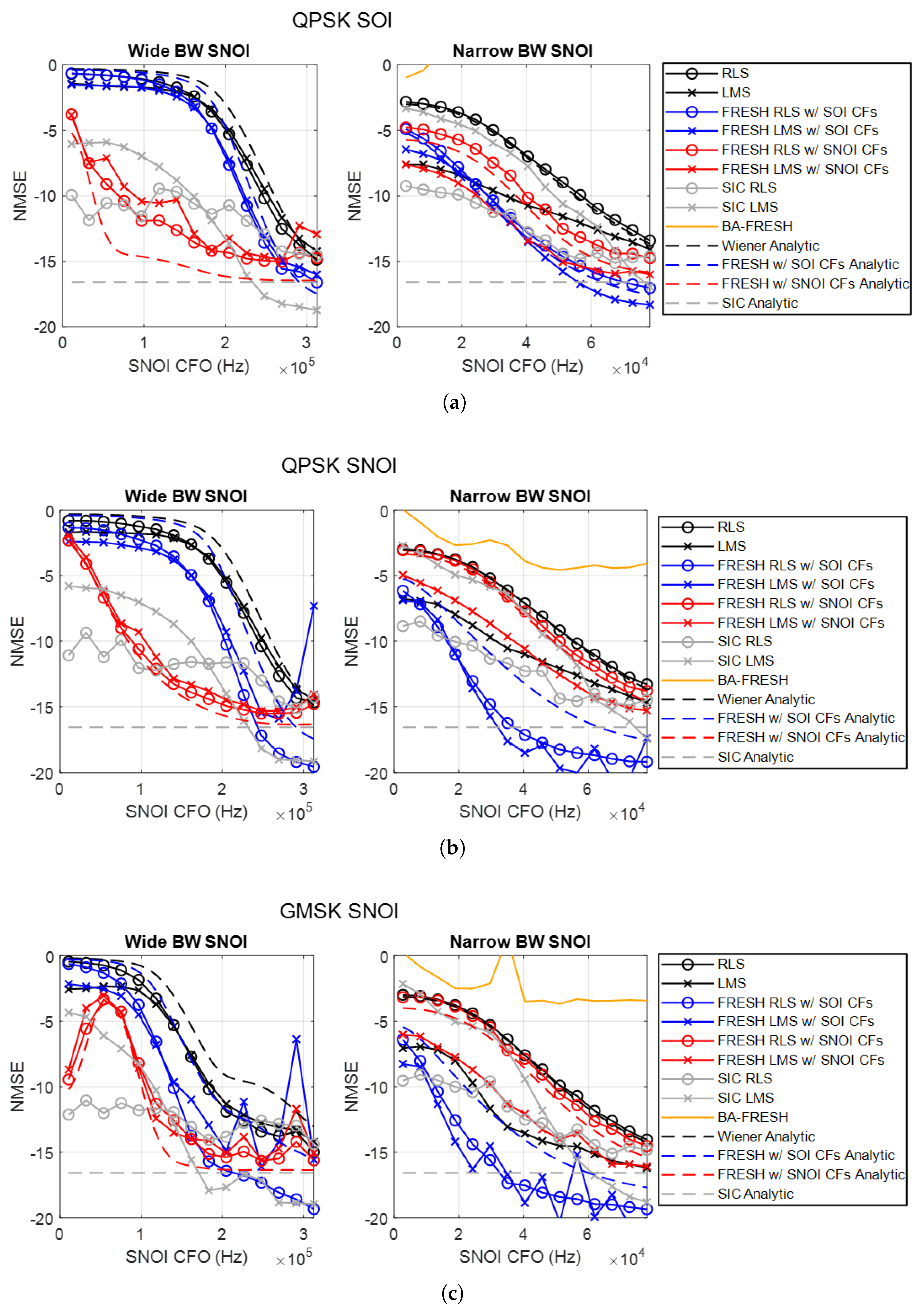
Figure A2.
Supplementary results of the SDR experiments. Comparison of BER when the modulation is varied. Figure (a) shows the results of a QPSK SOI, Figure (b) shows the results of a QPSK SNOI and Figure (c) shows the results of a GMSK SNOI.
References
- Bukhari, J.; Mérida, W. 5G interference with aviation altimeters: Technology and policy recommendations for coexistence. Transp. Policy 2024, 153, 1–11. [Google Scholar] [CrossRef] [Scilit]
- Rao, M.; O’Driscoll, C.; Borio, D.; Fortuny, J. LightSquared effects on estimated C/N 0, pseudoranges and positions. GPS Solut. 2014, 18, 1–13. [Google Scholar] [CrossRef] [Scilit]
- Hu, Y.; Xia, W.; Shen, L. Study of anti-interference mechanisms of multiple WPANs accessing into a HAN. In Proceedings of the 2007 International Symposium on Intelligent Signal Processing and Communication Systems, Xiamen, China, 28 November–1 December 2007; pp. 810–813. [Google Scholar]
- Enehizena, O.N.; Aigbodion, D.O.; Ogbeide, K.O.; Imoize, A.L.; Mejdoub, Y. Advancements in Cross-Technology Coexistence: A Critical Review of SledZig for ZigBee and Wi-Fi Interference Mitigation. In Proceedings of the International Conference on Connected Objects and Artificial Intelligence; Springer: Berlin/Heidelberg, Germany, 2025; pp. 64–69. [Google Scholar]
- IEEE Std 802.15.4; IEEE Standard for Low-Rate Wireless Networks. IEEE: New York, NY, USA, 2024.
- Higuchi, K.; Benjebbour, A. Non-orthogonal multiple access (NOMA) with successive interference cancellation for future radio access. IEICE Trans. Commun. 2015, 98, 403–414. [Google Scholar] [CrossRef] [Scilit]
- Iswarya, N.; Jayashree, L. A survey on successive interference cancellation schemes in non-orthogonal multiple access for future radio access. Wirel. Pers. Commun. 2021, 120, 1057–1078. [Google Scholar] [CrossRef] [Scilit]
- Chew, D.; Nguyen, C.; Berhanu, S.; Baumgart, C.; Cooper, A.B. Covert Communications through Imperfect Cancellation. In Proceedings of the 2022 ACM Workshop on Information Hiding and Multimedia Security; ACM: New York, NY, USA, 2022; pp. 63–68. [Google Scholar] [CrossRef] [Scilit]
- Agee, B.; Schell, S.; Gardner, W. The SCORE approach to blind adaptive signal extraction: An application of the theory of spectral correlation. In Proceedings of the Fourth IEEE ASSP Workshop on Spectral Estimation and Modeling, Minneapolis, MN, USA, 3–5 August 1988; pp. 3–5. [Google Scholar]
- Schell, S.V.; Agee, B. Application of the SCORE algorithm and SCORE extensions to sorting in the rank-L spectral self-coherence environment. In Proceedings of the Twenty-Second Asilomar Conference on Signals, Systems and Computers; IEEE Computer Society: New York, NY, USA, 1988; Volume 1, pp. 274–275. [Google Scholar]
- Napolitano, A. Cyclostationary Processes and Time Series: Theory, Applications, and Generalizations; Academic Press: Cambridge, MA, USA, 2019. [Google Scholar]
- Ingle, V.; Kogon, S.; Manolakis, D. Statistical and Adaptive Signal Processing; Artech: Norwood, MA, USA, 2005. [Google Scholar]
- Gardner, W. Cyclic Wiener filtering: Theory and method. IEEE Trans. Commun. 1993, 41, 151–163. [Google Scholar] [CrossRef] [Scilit]
- Reed, J.H.; Hsia, T.C. The performance of time-dependent adaptive filters for interference rejection. IEEE Trans. Acoust. Speech Signal Process. 1990, 38, 1373–1385. [Google Scholar] [CrossRef] [Scilit]
- Han, B.W.; Cho, J.H. Capacity of Second-Order Cyclostationary Complex Gaussian Noise Channels. IEEE Trans. Commun. 2012, 60, 89–100. [Google Scholar] [CrossRef] [Scilit]
- Reed, J.H. Time-Dependent Adaptive Filters for Interference Rejection; University of California: Oakland, CA, USA, 1987. [Google Scholar]
- Mendoza, R.; Reed, J.; Hsia, T.; Agee, B. Interference rejection using the time-dependent constant modulus algorithm (CMA) and the hybrid CMA/spectral correlation discriminator. IEEE Trans. Signal Process. 1991, 39, 2108–2111. [Google Scholar] [CrossRef] [Scilit] [PubMed]
- Jauhar, A. A CMA-FRESH Whitening Filter for Blind Interference Rejection. Doctoral Dissertation, Virginia Tech, Blacksburg, VA, USA, 2018. [Google Scholar]
- Yeung, G. Blind-adaptive linear frequency-shift filtering. Representations 1994, 50, 1. [Google Scholar]
- Zhang, J.; Wong, K.; Jin, Q.; Wu, Q. A new kind of adaptive frequency shift filter. In Proceedings of the 1995 International Conference on Acoustics, Speech, and Signal Processing; IEEE: New York, NY, USA, 1995; Volume 2, pp. 913–916. [Google Scholar]
- Saggar, H.; Mehra, D. Cyclostationary spectrum sensing in cognitive radios using fresh filters. arXiv 2013, arXiv:1312.5257. [Google Scholar]
- Chopra, R.; Ghosh, D.; Mehra, D.K. Spectrum Sensing for Cognitive Radios Based on Space-Time FRESH Filtering. IEEE Trans. Wirel. Commun. 2014, 13, 3903–3913. [Google Scholar] [CrossRef] [Scilit]
- Ribhu; Ghosh, D.; Mehra, D. Cooperative spectrum sensing for cognitive radios using jointly adaptive FRESH filters. In Proceedings of the 2015 Twenty First National Conference on Communications (NCC), Mumbai, India, 27 February–1 March 2015; pp. 1–6. [Google Scholar]
- Garakyaragh, N.; Shahtalebi, K.; Forouzan, A.R. A Cyclic Frequency Tracking Loop for Wideband Spectrum Sensing and FM Demodulation. IEEE Commun. Lett. 2016, 20, 2015–2018. [Google Scholar] [CrossRef] [Scilit]
- Agee, B.G.; Schell, S.V.; Gardner, W.A. Spectral self-coherence restoral: A new approach to blind adaptive signal extraction using antenna arrays. Proc. IEEE 2002, 78, 753–767. [Google Scholar]
- Gardner, W.; Reed, C. Making the most out of spectral redundancy in GSM: Cheap CCI suppression. In Proceedings of the Conference Record of Thirty-Fifth Asilomar Conference on Signals, Systems and Computers (Cat. No. 01CH37256); IEEE: New York, NY, USA, 2001; Volume 1, pp. 883–889. [Google Scholar]
- Gardner, W. Suppression of cochannel interference in GSM by pre-demodulation signal processing. In Proceedings of the 11th Virginia Tech Symposium on Wireless Personal Communications, Blacksburg, VA, USA, 9–11 June 2001. [Google Scholar]
- Garakyaragh, N.; Shahtalebi, K. Adaptive FRESH filter with vicarious reference for interference rejection: An application to signal detection in NOMA system. Trans. Emerg. Telecommun. Technol. 2022, 33, e4582. [Google Scholar] [CrossRef] [Scilit]
- Datta, J.; Lin, H.P. Detection of uplink NOMA systems using joint SIC and cyclic FRESH filtering. In Proceedings of the 2018 27th Wireless and Optical Communication Conference (WOCC), Hualien, Taiwan, 30 April–1 May 2018; pp. 1–4. [Google Scholar]
- Carrick, M.; Reed, J.H.; Harris, F. An optimal filter for signals with time-varying cyclostationary statistics. In Proceedings of the 2017 22nd International Conference on Digital Signal Processing (DSP), London, UK, 23–25 August 2017; pp. 1–5. [Google Scholar]
- Carrick, M.; Reed, J.; Spooner, C. Paramorphic multicarrier communications for interference mitigation. EURASIP J. Adv. Signal Process. 2018, 2018, 1687–6180. [Google Scholar] [CrossRef] [Scilit]
- Carrick, M.; Reed, J.H. Exploiting the cyclostationarity of radar chirp signals with time-varying filters. In Proceedings of the 2017 IEEE Global Conference on Signal and Information Processing (GlobalSIP), Montreal, QC, Canada, 14–16 November 2017; pp. 274–277. [Google Scholar]
- Carrick, M.; Reed, J.H.; Spooner, C.M. Mitigating Linear-Frequency-Modulated Pulsed Radar Interference to OFDM. IEEE Trans. Aerosp. Electron. Syst. 2019, 55, 1146–1159. [Google Scholar] [CrossRef] [Scilit]
- Fhima, H.; Zayani, R.; Shaiek, H.; Roviras, D.; Chang, B.S.; Bouallegue, R. Comparison of Linear, Widely Linear and Fresh Equalizers for FBMC-OQAM Systems with Different Numerologies. Wirel. Pers. Commun. 2020, 115. [Google Scholar] [CrossRef] [Scilit]
- Spooner, C.M.; Gardner, W.A. Cubic Frequency-Shift Filtering for Cochannel Interference Removal; Technical Report; University of California: Davis, CA, USA, 1993. [Google Scholar]
- IEEE Std 1901.2; Standard for Low-Frequency (Less than 500 kHz) Narrowband Power Line Communications for Smart Grid Applications. IEEE: New York, NY, USA, 2013.
- Shlezinger, N.; Dabora, R. Frequency-Shift Filtering for OFDM Signal Recovery in Narrowband Power Line Communications. IEEE Trans. Commun. 2014, 62, 1283–1295. [Google Scholar] [CrossRef] [Scilit]
- Elgenedy, M.; Sayed, M.; Al-Dhahir, N.; Chabaan, R.C. Cyclostationary Noise Mitigation for SIMO Powerline Communications. IEEE Access 2018, 6, 5460–5484. [Google Scholar] [CrossRef] [Scilit]
- Elgenedy, M. Enhancing Rate and Reliability of PLC in LV/MV Smart Grid Networks. Ph.D. Thesis, The University of Texas at Dallas, Dallas, TX, USA, 2019. [Google Scholar]
- Chien, Y.; Lin, J.; Tsao, H. Cyclostationary impulsive noise mitigation in the presence of cyclic frequency offset for narrowband powerline communication systems. Electronics 2020, 9, 988. [Google Scholar] [CrossRef] [Scilit]
- Chien, Y.; Xu, S.; Lu, S. Cyclostationary impulsive noise mitigation algorithm for narrowband powerline communications. J. Frankl. Inst. 2020, 357, 687–703. [Google Scholar] [CrossRef] [Scilit]
- Li, F.; Han, X.; Li, Y.; Long, T. Interrupted-sampling repeater jamming (ISRJ) suppression based on cyclostationarity. In Proceedings of the IET Conference Proceedings CP779; IET: Stevenage, UK, 2020; Volume 2020, pp. 793–797. [Google Scholar]
- Liu, H.; Li, J.; Lu, S.; Li, F.; Zhang, L. Interrupted-Sampling Repeater Jamming (ISRJ) suppression method based on segmented FRESH filtering target detection. In Proceedings of the IET International Radar Conference (IRC 2023); IET Conference Proceedings: Stevenage, UK, 2023; Volume 2023, pp. 594–600. [Google Scholar] [CrossRef] [Scilit]
- Yong, C.; Tao, L. Application study of BA-FRESH filtering technique for communication anti-jamming. In Proceedings of the IEEE 10th International Conference on Signal Processing Proceedings; IEEE: New York, NY, USA, 2010; pp. 287–290. [Google Scholar]
- Chen, X.; Yang, W. Detection of Jamming in DSSS Systems Using FRESH Filters. In Proceedings of the 2020 IEEE 3rd International Conference of Safe Production and Informatization (IICSPI), Chongqing, China, 28–30 November 2020; pp. 320–325. [Google Scholar]
- Dobre, O.; Bar-Ness, Y.; Su, W. Higher-order cyclic cumulants for high order modulation classification. In Proceedings of the IEEE Military Communications Conference, 2003; MILCOM 2003; IEEE: New York, NY, USA, 2003; Volume 1, pp. 112–117. [Google Scholar] [CrossRef] [Scilit]
- Napolitano, A.; Spooner, C. Cyclic spectral analysis of continuous-phase modulated signals. IEEE Trans. Signal Process. 2001, 49, 30–44. [Google Scholar] [CrossRef]
- Chew, D.; Berhanu, S.; Baumgart, C.; Cooper, A.B. Improved OFDM Signal Cancellation through Window Estimation. arXiv 2023, arXiv:2303.12472. [Google Scholar]
- Benjebbour, A.; Asai, T.; Yoshino, H. Pulse shape design for efficient rejection of unknown in-band interference using cyclic Wiener filtering. In Proceedings of the IEEE Vehicular Technology Conference; IEEE: New York, NY, USA, 2006; pp. 1–5. [Google Scholar]
- Zhang, J.; Wong, K.; Luo, Z.; Ching, P. Blind adaptive FRESH filtering for signal extraction. IEEE Trans. Signal Process. 1999, 47, 1397–1402. [Google Scholar] [CrossRef] [Scilit]
- Ojeda, O. Adaptive-FRESH filters for compensation of cycle-frequency errors. IEEE Trans. Signal Process. 2009, 10, 1–10. [Google Scholar] [CrossRef] [Scilit]
- Cai, X.; Wang, X.; Huang, Z.T.; Wang, F.H. Single channel steepest descent algorithm for the correction of cycle frequency error. IET Commun. 2016, 10, 1829–1838. [Google Scholar] [CrossRef] [Scilit]
- Yuan, L.; Pan, J.; Yang, N.; Ding, Z.; Yuan, J. Successive Interference Cancellation for LDPC Coded Nonorthogonal Multiple Access Systems. IEEE Trans. Veh. Technol. 2018, 67, 5460–5464. [Google Scholar] [CrossRef] [Scilit]
- Strassle, C.; Megnet, D.; Mathis, H.; Burgi, C. The squaring-loss paradox. In Proceedings of the 20th International Technical Meeting of the Satellite Division of the Institute of Navigation (ION GNSS 2007), Fort Worth, TX, USA, 25–28 September 2007; pp. 2715–2722. [Google Scholar]
- Sklar, B. Digital Communications: Fundamentals and Applications; Pearson: Hong Kong, China, 2021. [Google Scholar]
- Horowitz, M. 1.1 Computing’s energy problem (and what we can do about it). In Proceedings of the 2014 IEEE International Solid-State Circuits Conference Digest of Technical Papers (ISSCC), San Francisco, CA, USA, 9–13 February 2014; pp. 10–14. [Google Scholar] [CrossRef] [Scilit]
- Kim, K.; Akbar, I.A.; Bae, K.K.; Um, J.S.; Spooner, C.M.; Reed, J.H. Cyclostationary Approaches to Signal Detection and Classification in Cognitive Radio. In Proceedings of the 2007 2nd IEEE International Symposium on New Frontiers in Dynamic Spectrum Access Networks, Dublin, Ireland, 17–20 April 2007; pp. 212–215. [Google Scholar] [CrossRef] [Scilit]
- Dandawate, A.; Giannakis, G. Statistical tests for presence of cyclostationarity. IEEE Trans. Signal Process. 1994, 42, 2355–2369. [Google Scholar] [CrossRef] [Scilit]
- Spooner, C.M. Performance Evaluation of Detectors for Cyclostationary Signals; University of California: Davis, CA, USA, 1988. [Google Scholar]
- Spooner, C. Frequency Shift (FRESH) Filtering for Single-Sensor Cochannel Signal Separation. 2023. Available online: https://cyclostationary.blog/2023/03/01/frequency-shift-fresh-filtering-for-single-sensor-cochannel-signal-separation/ (accessed on 30 April 2026).
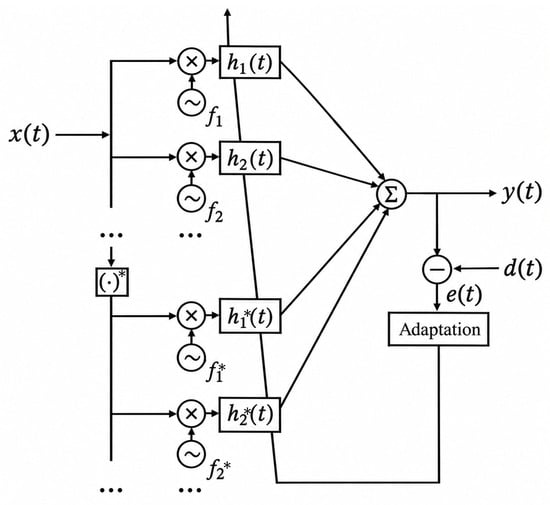
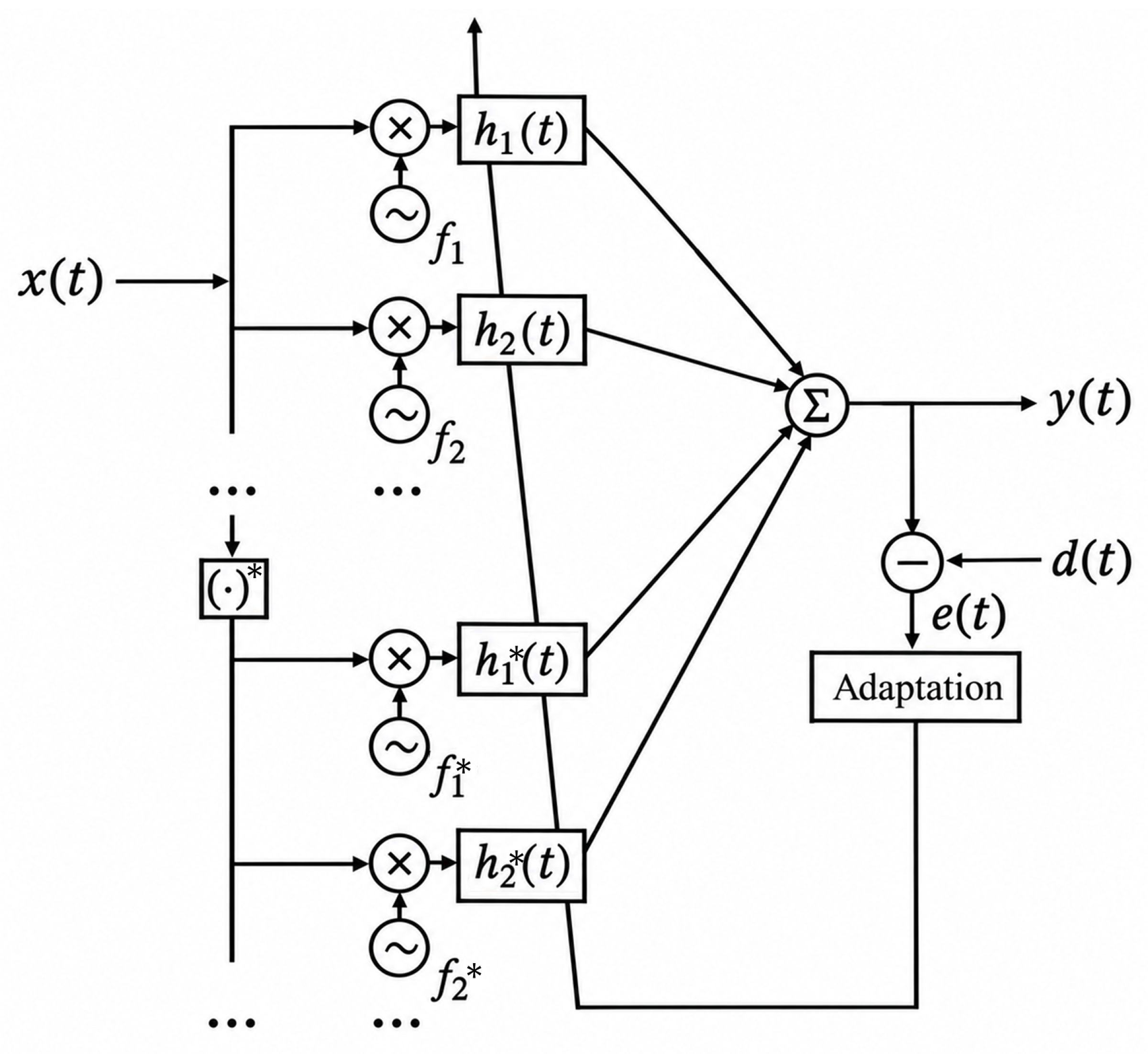
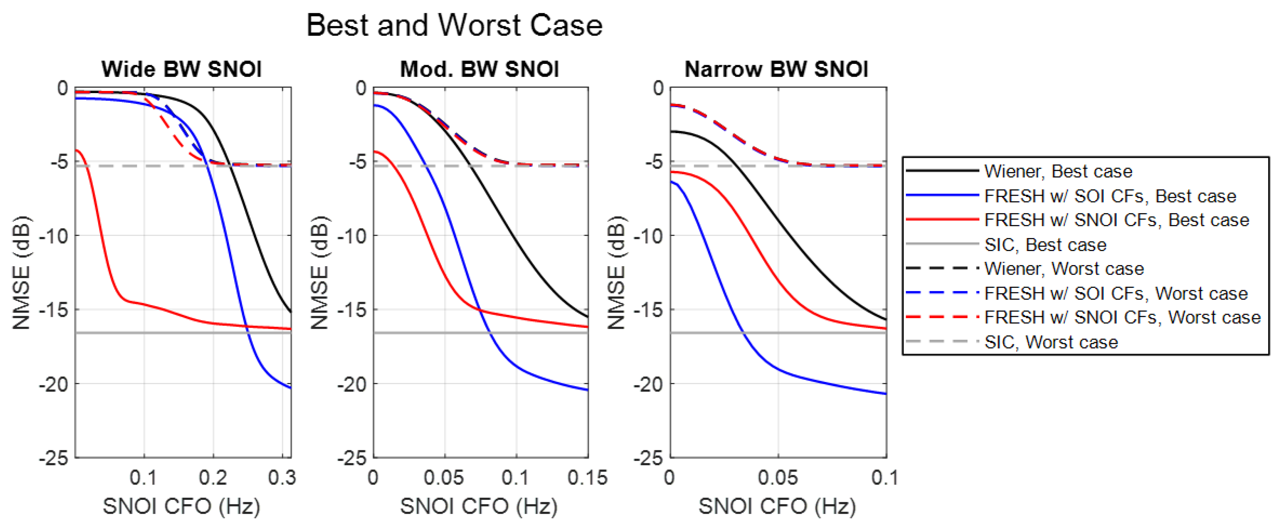
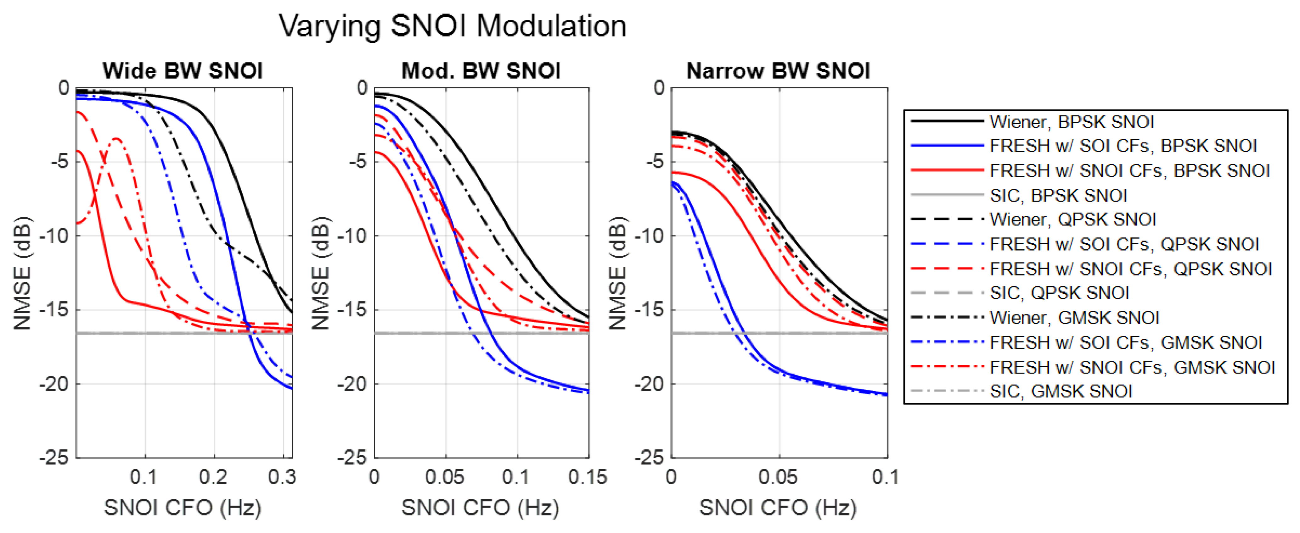
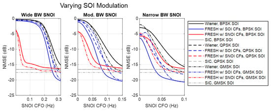
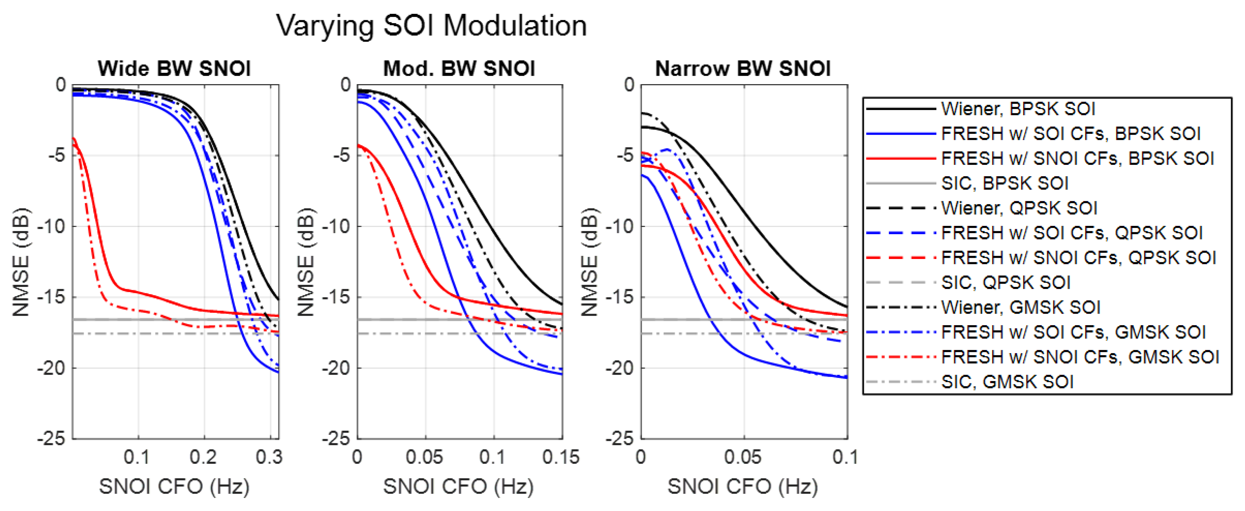
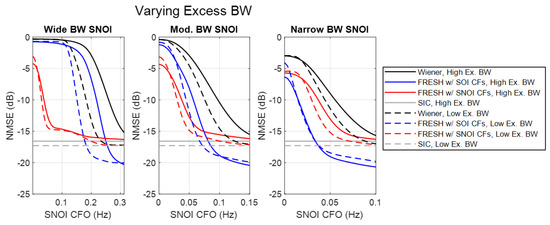
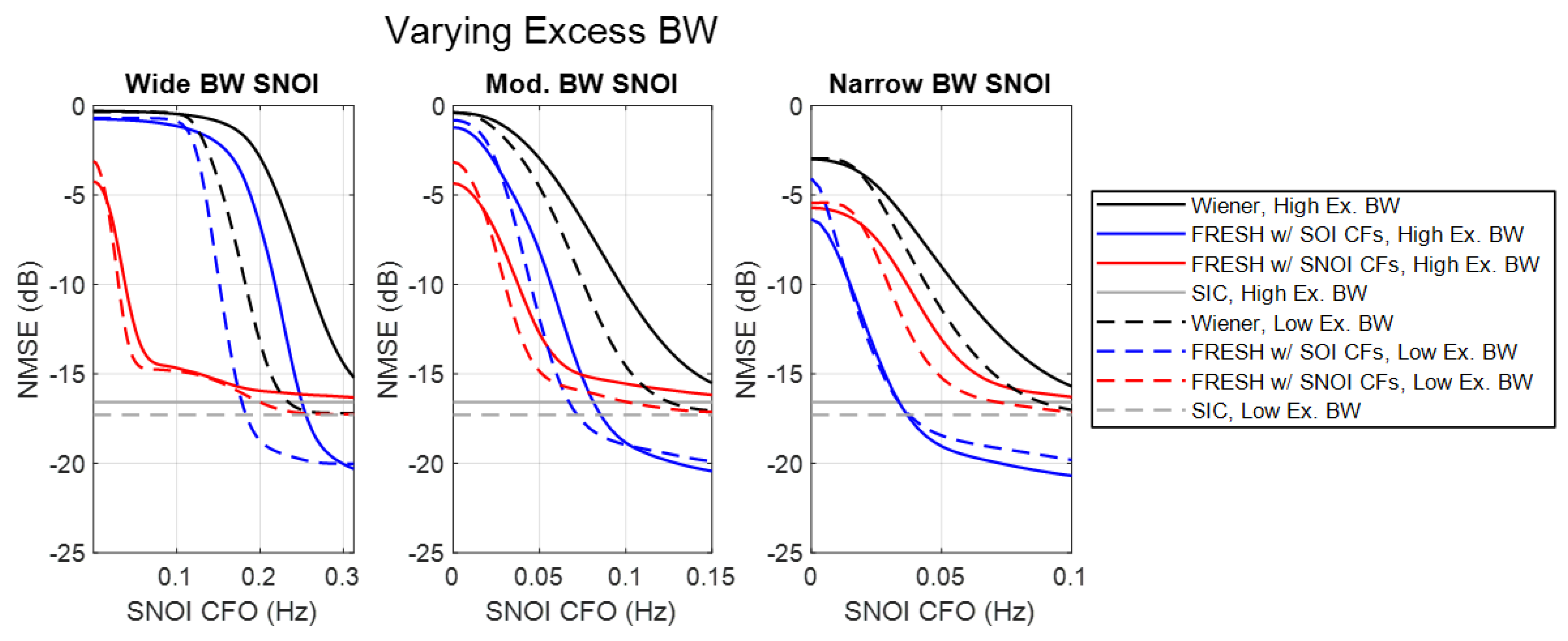
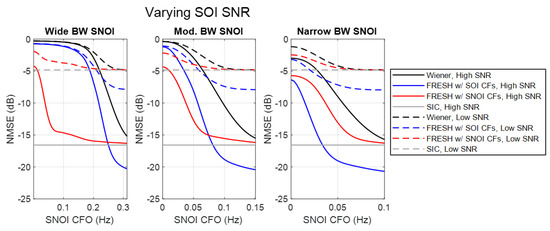
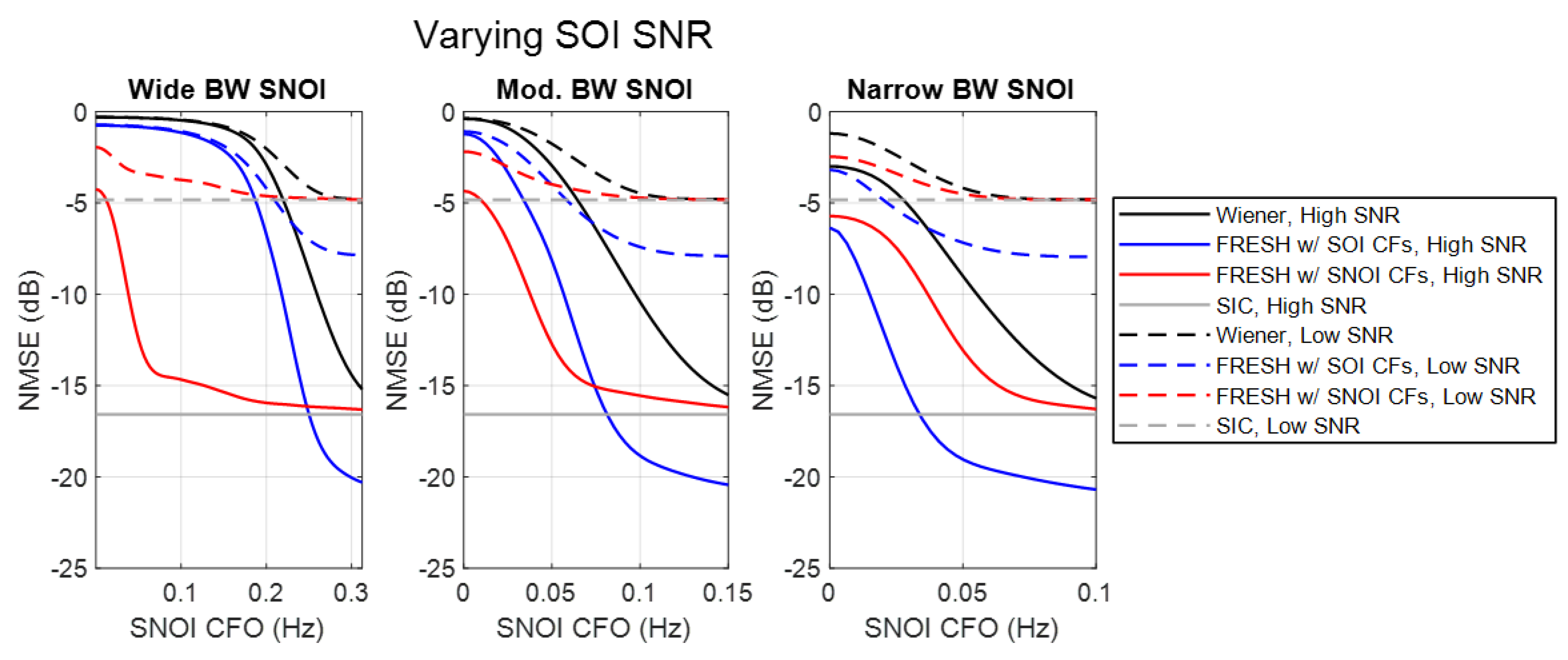
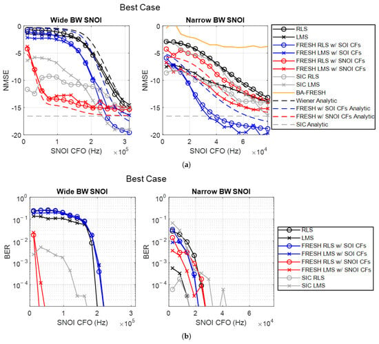
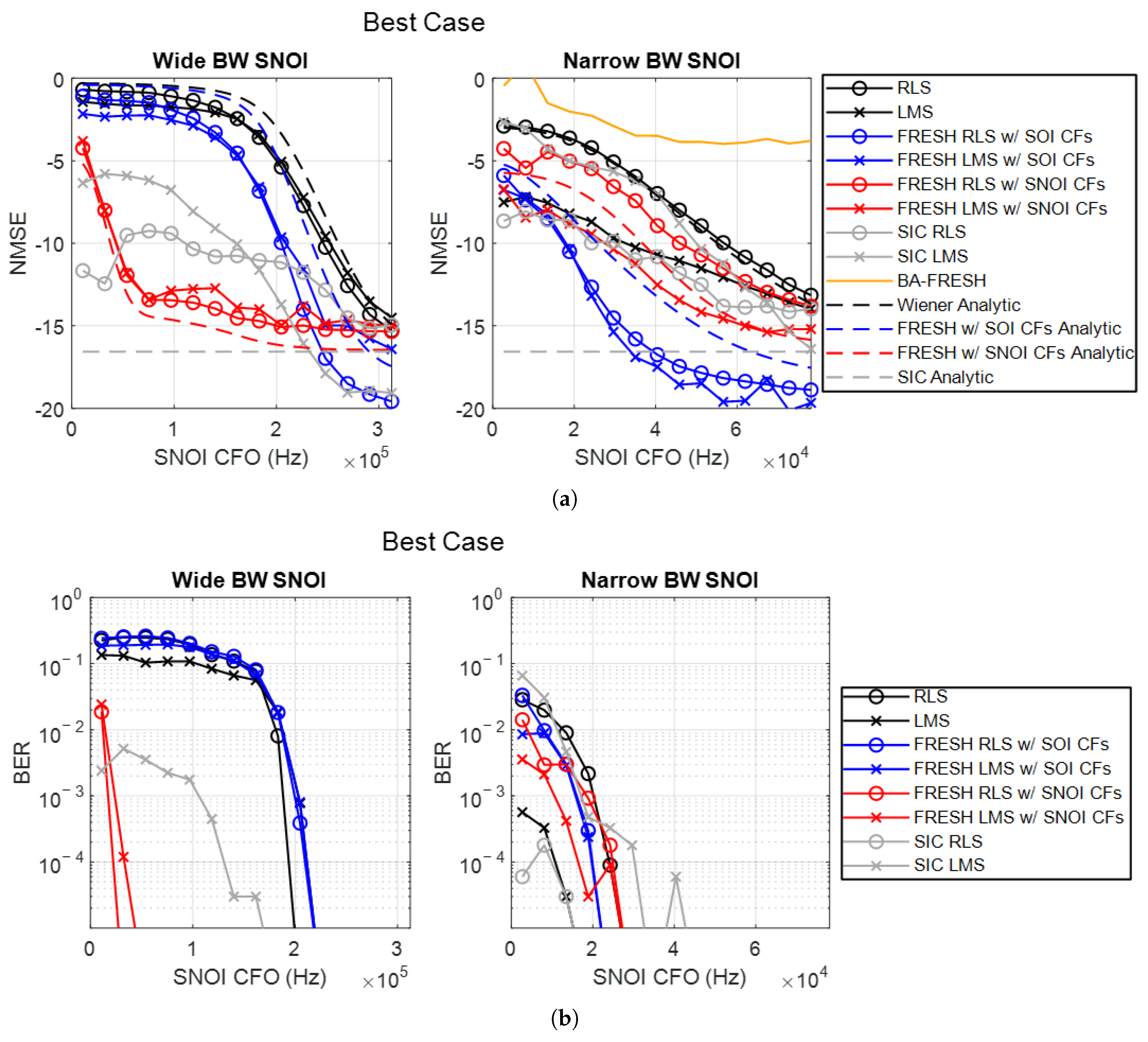
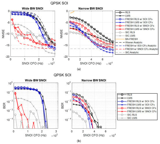
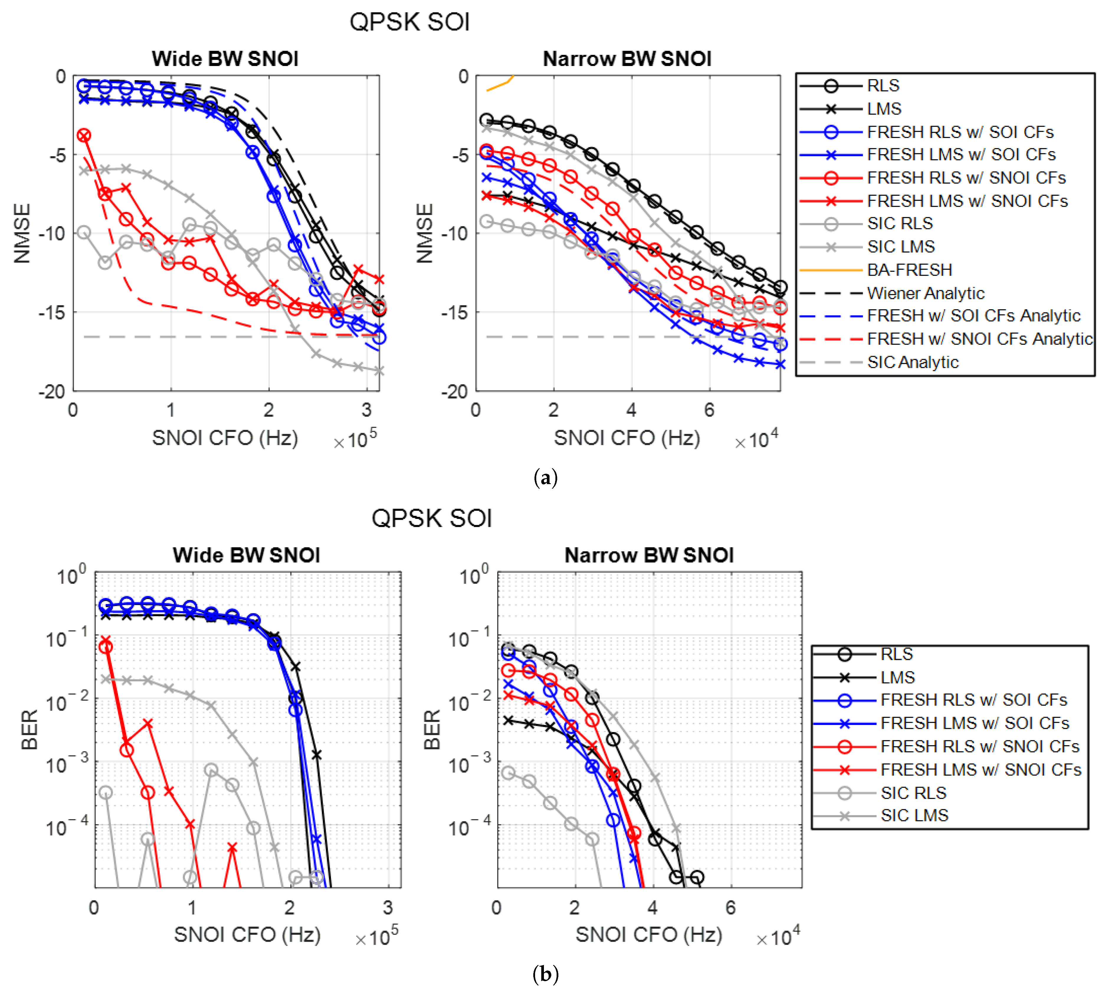
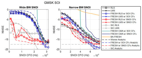
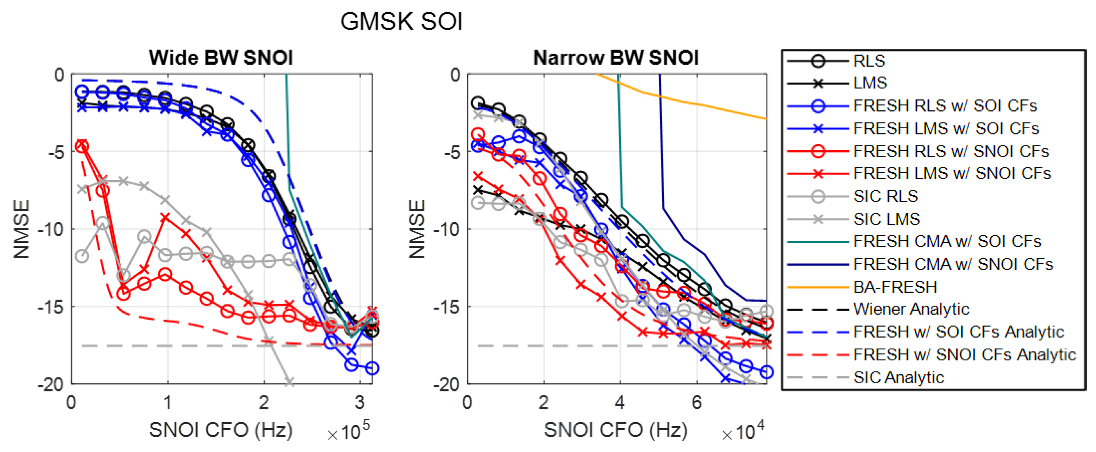
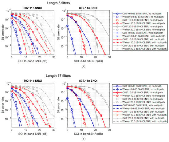
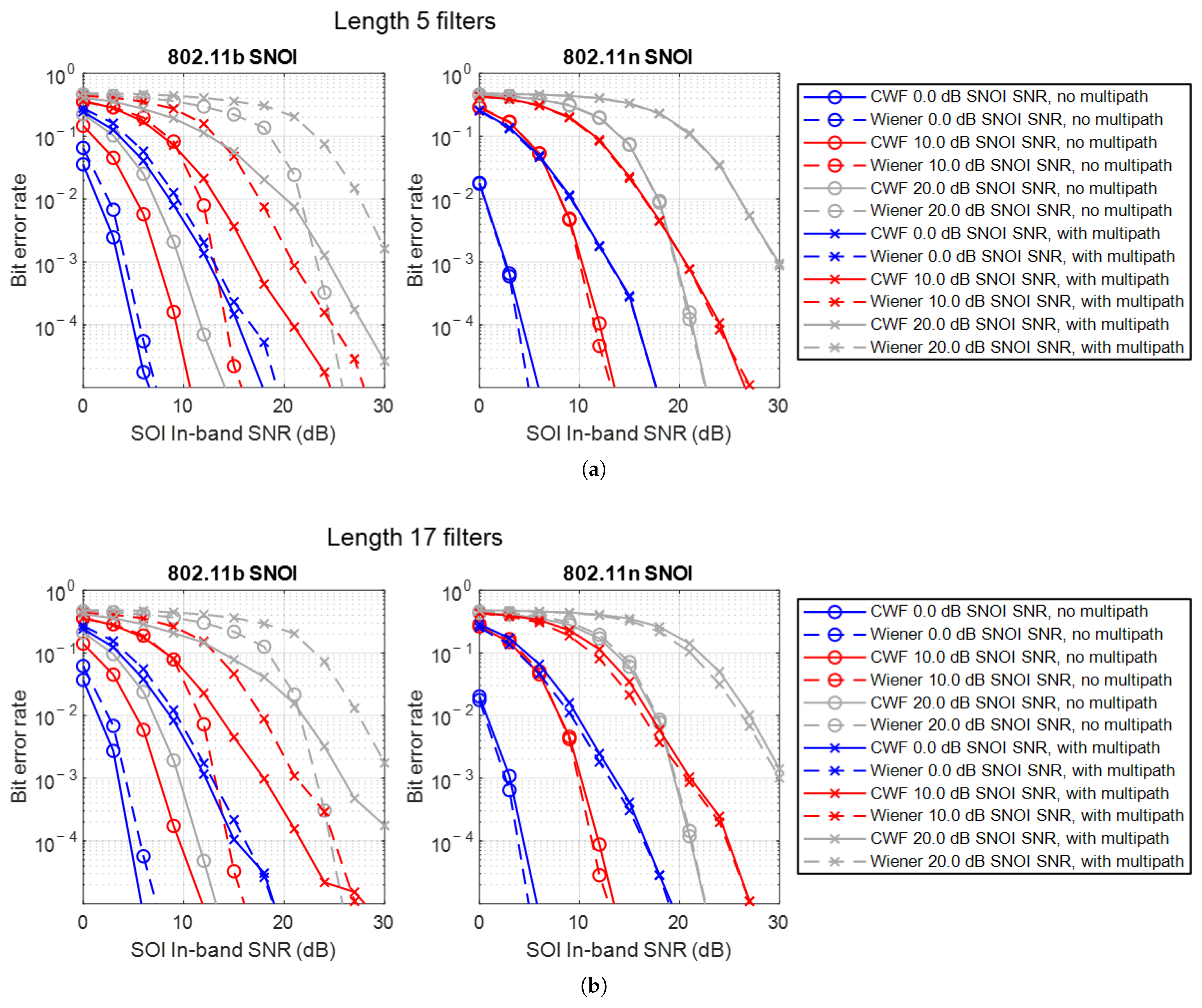
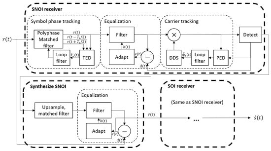
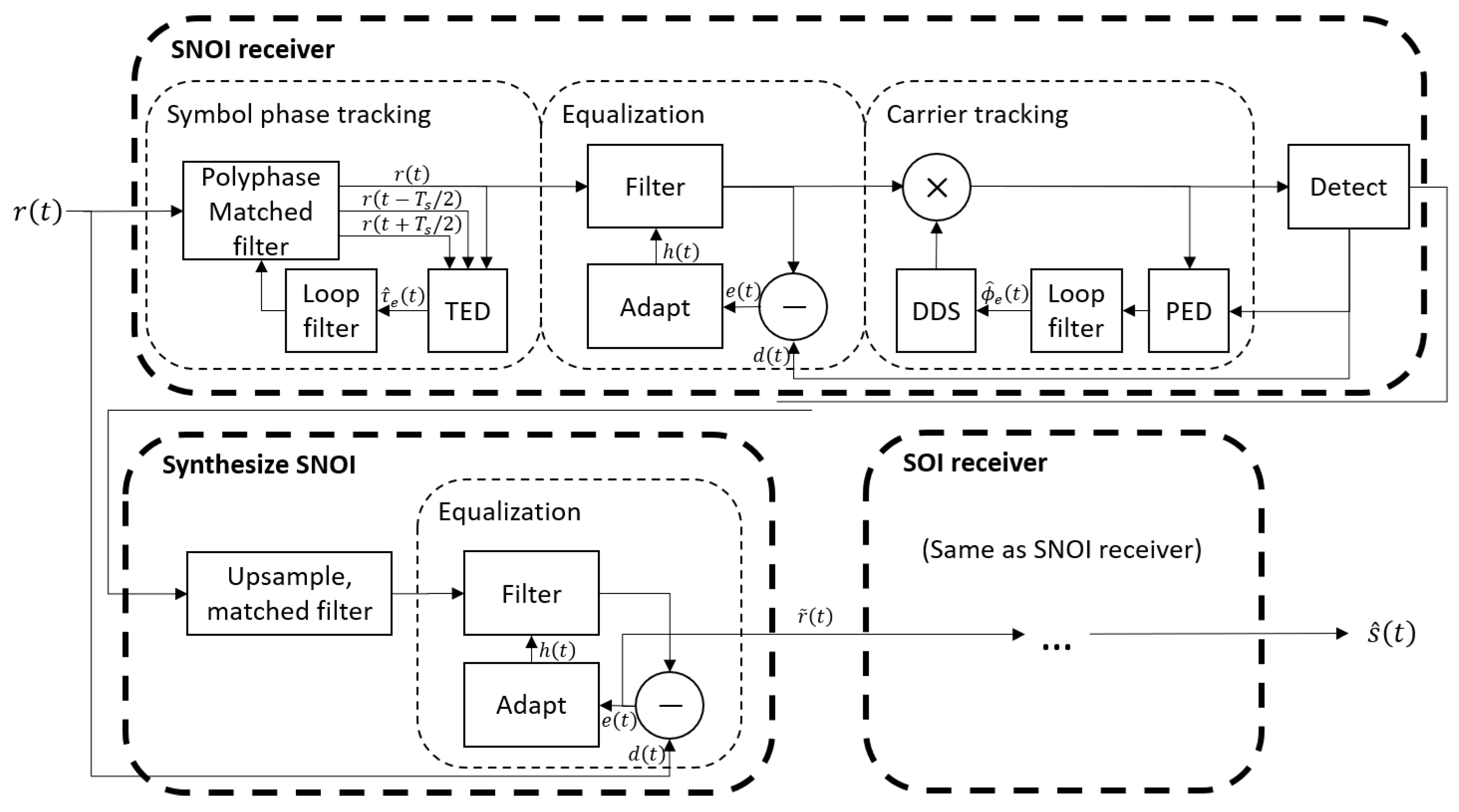
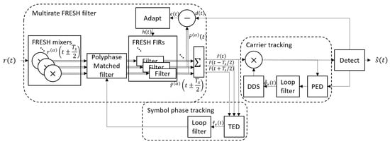
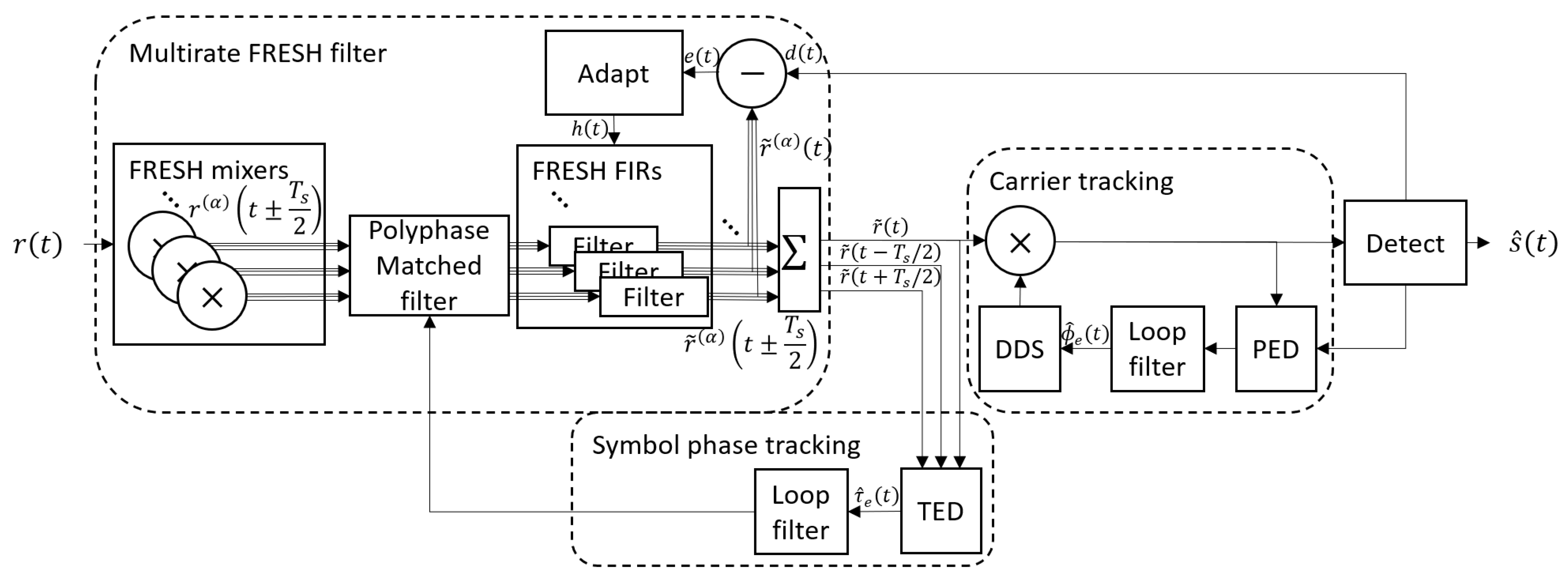
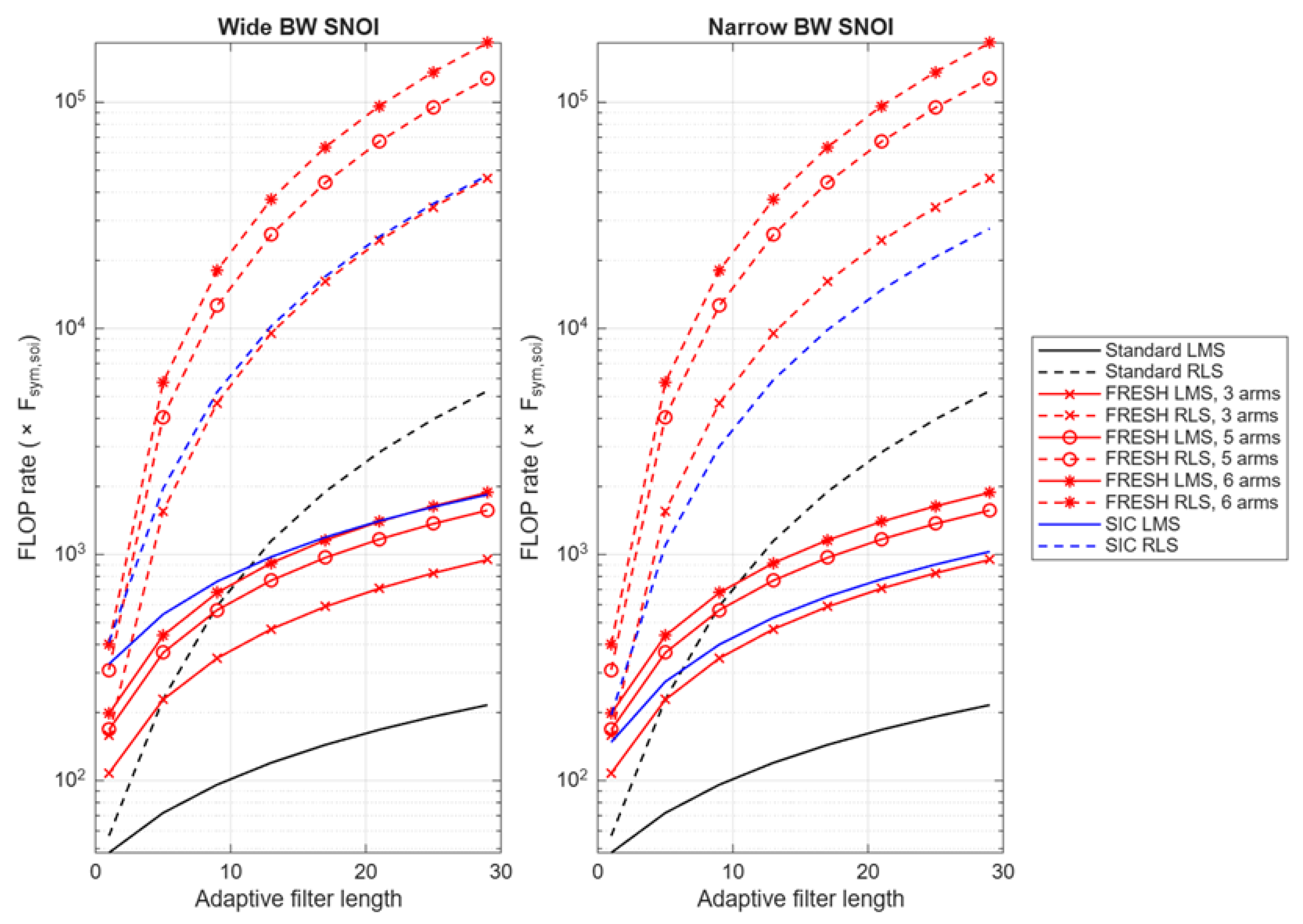

Disclaimer/Publisher’s Note: The statements, opinions and data contained in all publications are solely those of the individual author(s) and contributor(s) and not of MDPI and/or the editor(s). MDPI and/or the editor(s) disclaim responsibility for any injury to people or property resulting from any ideas, methods, instructions or products referred to in the content. |
© 2026 by the authors. Licensee MDPI, Basel, Switzerland. This article is an open access article distributed under the terms and conditions of the Creative Commons Attribution (CC BY) license.